![NHP: Neural Hypergraph Link Prediction · hyperlinks E−E. The state-of-the art method for the problem is the co-ordinated matrix minimisation (CMM) algorithm [44] and uses the expectation-maximisation](https://static.fdocuments.in/doc/165x107/601991ed1431f002d9784b84/nhp-neural-hypergraph-link-prediction-hyperlinks-eae-the-state-of-the-art-method.jpg)
1 Topic 6: Optimization I Maximisation and Minimisation Jacques (4th Edition): Chapter 4.6 & 4.7.
31
1 Topic 6: Optimization I Maximisation and Minimisation Jacques (4th Edition): Chapter 4.6 & 4.7
-
date post
18-Dec-2015 -
Category
Documents
-
view
222 -
download
0
Transcript of 1 Topic 6: Optimization I Maximisation and Minimisation Jacques (4th Edition): Chapter 4.6 & 4.7.

1
Topic 6: Optimization I
Maximisation and Minimisation
Jacques (4th Edition):
Chapter 4.6 & 4.7

2
For a straight line Y=a+bX Y= f (X) = a + bX
First Derivative dY/dX = f = b
constant slope b
Second Derivative d2Y/dX2 = f = 0
constant rate of change - the change in the slope is zero - (i.e. change in Y due to change in X does not depend on X)
Y
X
a

3
Y
X
Y=X >1
X
Y Y=X 0< < 1
For non-linear functions

4
Y= f (X) = X
First Derivative
dY/dX = f = X-1 > 0
Positive Slope: change in Y due to change X is Positive
Second Derivative
d2Y/dX2 = f = (-1) X(-1)-1 or
d2Y/dX2 = f = (-1)(Y/X2)
5
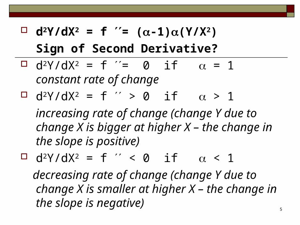
d2Y/dX2 = f = (-1)(Y/X2)
Sign of Second Derivative? d2Y/dX2 = f = 0 if = 1 constant rate of
change d2Y/dX2 = f > 0 if > 1
increasing rate of change (change Y due to change X is bigger at higher X – the change in the slope is positive)
d2Y/dX2 = f < 0 if < 1
decreasing rate of change (change Y due to change X is smaller at higher X – the change in the slope is negative)
6
Maximisation and Minimisation
Stationary Points
•Second-order derivatives
•Applications

7
Y
If f (X) < 0 as X will Y
If f (X) > 0 as X will Y
If f (X) = 0 slope 0…as X no change Y
X*=1
A
B

8
Definition
Stationary points are the turning points or critical points of a function
Slope of tangent to curve is zero at stationary points
Stationary point(s) at A & B: where f (X) = 0

9
Are these a Max or Min point of the function?
1) examine slope in region near the stationary point
Sign of first derivative around a turning point: Before At After Maximum plus zero minus Minimum minus zero plus
dY/dX = f (X) is (–, 0, +) min dY/dX = f (X) is (+, 0, -) max

10
if d2Y/dX2 = f (X) > 0 a minimum the change in the slope is positive beyond the stationary point, so the point is a local minimum
if d2Y/dX2 = f (X) < 0 a maximum the change in the slope is negative beyond the stationary point, so the point is a local maximum
if d2Y/dX2 = f (X) = 0 indeterminate the change in the slope is zero beyond the stationary point - could be a max, or a min, or an inflection point
2) or calculate the second derivative……
look at the change in the slope beyond the stationary point

11
e.g. inflection point
f =0 & f =0

12
To find the Max or Min of a function Y= f(X)
1) First Order Condition (F.O.C.):
set slope dY/dX = f (X) = 0
this identifies the stationary point(s)
2) Second Order Condition (S.O.C.):
check the sign of the second derivative (gives the change in the slope)
d2Y/dX2 = f (X) > 0 a minimum
d2Y/dX2 = f (X) < 0 a maximum d2Y/dX2 = f (X) = 0 indeterminate
this identifies whether the slope of the function is increasing, decreasing, or does not change after the stationary point(s)
13
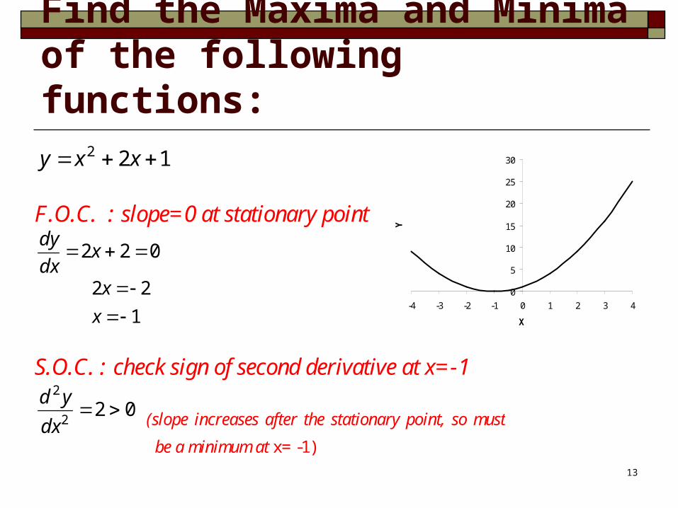
Find the Maxima and Minima of the following functions:
122 xxy F.O.C. : slope=0 at stationary point
022 xdx
dy
1
22
x
x
S.O.C. : check sign of second derivative at x=-1
022
2
dx
yd (slope increases after the stationary point, so must
be a minimum at x= -1)
0
5
10
15
20
25
30
-4 -3 -2 -1 0 1 2 3 4
X
Y

14
Example 1: Profit Maximisation
Question.
A firm faces the demand curveP=8-0.5Q
and total cost function TC=1/3Q3-3Q2+12Q.
Find the level of Q that maximises total profit and verify that this value of Q is where MC=MR

15
Answer….going to take a few slides!
Find Total Revenue….
P = 8 - 0.5Q inverse demand function
TR (Q) = P.Q = 8Q - ½Q2
TC (Q) = 1/3Q3 - 3Q2 + 12Q
Now write out the profit function
MAX = TR - TC (Q) = -4Q + 2 ½ Q2 – 1/3Q
3
The function we want to Maximise is PROFIT….
And Profit = Total Revenue – Total Cost
16
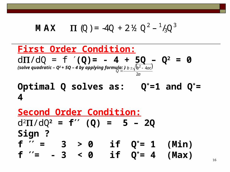
MAX (Q) = -4Q + 2 ½ Q2 – 1/3Q3
First Order Condition:d/dQ = f (Q)= - 4 + 5Q – Q2 = 0 (solve quadratic – Q2 + 5Q – 4 by applying formula: )
Optimal Q solves as: Q*=1 and Q*= 4
Second Order Condition:d2/dQ2 = f (Q) = 5 – 2Q Sign ? f = 3 > 0 if Q*= 1 (Min)f = - 3 < 0 if Q*= 4 (Max)
So profit is max at output Q = 4
a
acbbQ
2
42

17
Continued….. Verify that MR = MC at Q = 4:
TR (Q) = 8Q - ½Q2
MR = dTR/dQ = 8 – Q
Evaluate at Q = 4 …..then MR = 4
TC (Q) = 1/3Q3 - 3Q2 + 12Q
MC = dTC/dQ = Q2 – 6Q +12
Evaluate at Q = 4 ….
then MC = 16 – 24 +12 = +4
Thus At Q = 4, we have MR = MC
18
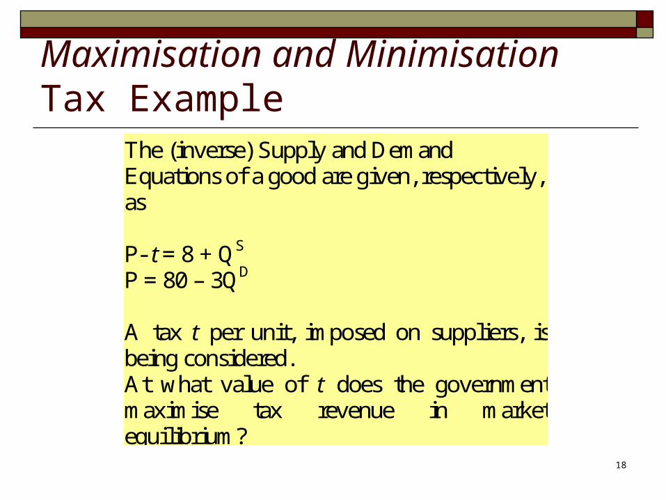
Maximisation and MinimisationTax Example
The (inverse) Supply and Demand Equations of a good are given, respectively, as P- t = 8 + QS P = 80 – 3QD A tax t per unit, imposed on suppliers, is being considered. At what value of t does the government maximise tax revenue in market equilibrium?

19
What do we want to maximise?Tax revenue in equilibrium…..
This will be equal to the tax rate t multiplied by the equilibrium quantity
So first we need to find the equilibrium quantity

20
Solution
To find equilibrium Q, Set Supply equal to Demand….
In equilibrium, QD = QS so
Q + 8 + t = 80 – 3Q
Now Solve for Q
Qe = 18 – ¼ t
Now we can write out our objective function…
Tax Revenue T = t.Qe = t(18 – ¼ t)
MAX T(t) = 18t – ¼ t2
t*

21
MAX T(t) = 18t – ¼ t2
t*
First Order Condition for max: set the slope (or first derivative) = 0
dT/dt = 18 – ½ t = 0
t* = 36
Second Order Condition for max: check sign of second derivative
d2T/dt2 = -½ < 0 at all values of x
Thus, tax rate of 36 will Maximise tax revenue in equilibrium

22
Now we can compute out the equilibrium P and Q and the total tax revenue when t = 36
At t* = 36
Qe = 18 – ¼ t* = 9
Tax Revenue T = t*.Qe = 18t* – ¼ t*2 = 324
Pe = Qe + 8 + t*= 53
If t = 0, then tax revenue = 0,
Qe = 18 ,
Pe = Qe + 8 = 26

23
Is the full burden of the tax passed on to consumers?
Ex-ante (no tax) Pe = 26
Ex-post (t* =36) Pe = 53
The tax is t*= 36, but the price increase is only 27 (75% paid by consumer)

24
Another example
Cost Producing Q output given capital K is: 22
8 QK
KC
(a) if K=20 in Short Run, find the level of Q at which AC is minimised.
(b) Show that MC and AC are equal at this point.

25
Solution Substituting in K = 20 to our C function:
C = (8*20) + (2/20)Q2 = 160 + 0.1Q2
AC = C/Q = 160/Q + 0.1Q
and MC = dC/dQ = 0.2Q
First Order Condition: set first derivative (slope)=0
AC is at min when dAC/dQ = 0
So dAC/dQ = - 160/Q2 + 0.1 = 0
And this solves as Q2 = 1600 Q = 40

26
Second Order Condition
Second Order Condition: check sign at Q = 40
If d2AC/dQ2 >0 min.
Since dAC/dQ = - 160/Q2 + 0.1
Then d2AC/dQ2 = + 320/Q3
Evaluate at Q = 40,
d2AC/dQ2 = 320 / 403 >0
min AC at Q = 40

27
b) Now show MC = AC when Q = 40:
AC = C/Q = 160/Q + 0.1Q
AC at Q=40: 160/40 + (0.1*40) = 8
and MC = dC/dQ = 0.2Q
So MC at Q = 40: 0.2*40 = 8
MC = AC at min AC when Q=40

28
c) What level of K minimises C when Q = 1000?
KKQ
KKC
functionCtoQSubstitute210002
8228
1000
)(
dC/dK = 8 – (2(10002 )/ K2 )= 0
Solving 8K2 = 2.(1000)2
K2 = ¼ .(1000)2
optimal K* = ¼.(1000)
=½(1000)=500
if Q = 1000, optimal K* = 500
more generally, if Q = Q0, optimal K = ½ Q0

29
Second Order Condition: check sign of second derivative at K = 500
If d2C/dK2 >0 min.
Since dC/dK = 8 – (2(10002 )/ K2 )
d2C/dK2 = + (2.(10002).2K )/ K4 >0 for all values of K>0 and so C are at a min when K = 500
The min cost producing Q =1000 occurs when K = 500
Subbing in value k = 500 we get C = 8000
or more generally, min cost producing Q0 occurs when K =
Q0/2 and so C = 4Q0 + 4Q0 = 8Q0

30
Topic 6: Maximisation and Minimisation Second DeIdentifying the max and min of various
functions Identifying the max and min of various functions –
sketch graphs Finding value of t that maximises tax revenues, given
D and S functions Identifying all local max and min of various
functions. Identifying profit max output level. Differentiate various functions.
31
Maximisation and Minimisation
Second-order derivatives Stationary Points Optimisation I Applications