1

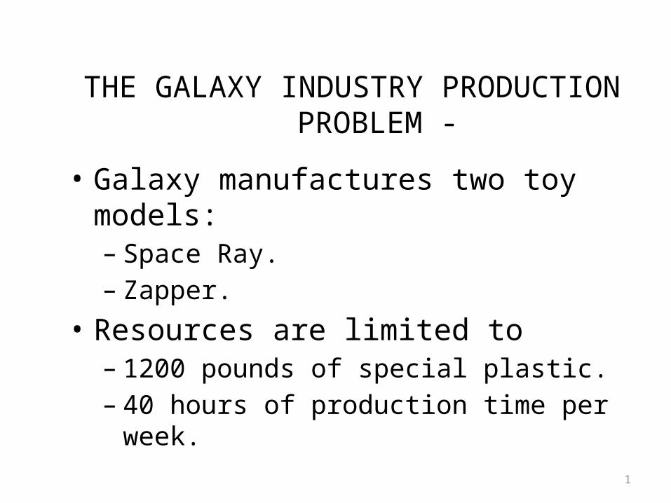
THE GALAXY INDUSTRY PRODUCTION PROBLEM -

• Galaxy manufactures two toy models:– Space Ray. – Zapper.

• Resources are limited to– 1200 pounds of special plastic.– 40 hours of production time per week.

2

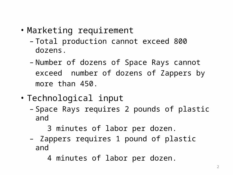
• Marketing requirement– Total production cannot exceed 800 dozens.

– Number of dozens of Space Rays cannot exceed number of dozens of Zappers by more than 450.

• Technological input– Space Rays requires 2 pounds of plastic and 3 minutes of labor per dozen.– Zappers requires 1 pound of plastic and 4 minutes of labor per dozen.

3

• Current production plan calls for:

– Producing as much as possible of the more profitable product, Space Ray ($8 profit per dozen).

– Use resources left over to produce Zappers ($5 profit per dozen).

• The current production plan consists of:

Space Rays = 550 dozens

Zapper = 100 dozens

Profit = 4900 dollars per week

4

Management is seeking a production schedule that will increase the company’s profit.

5

SOLUTION

• Decisions variables:– X1 = Production level of Space Rays (in dozens per

week).– X2 = Production level of Zappers (in dozens per

week).

• Objective Function:

– Weekly profit, to be maximized

6

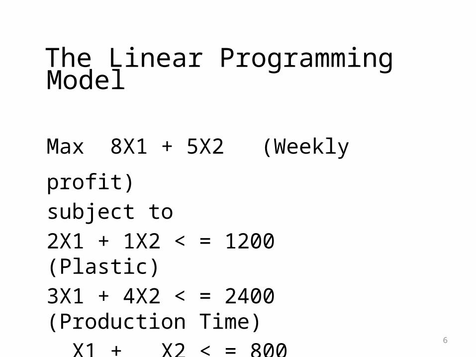
The Linear Programming Model

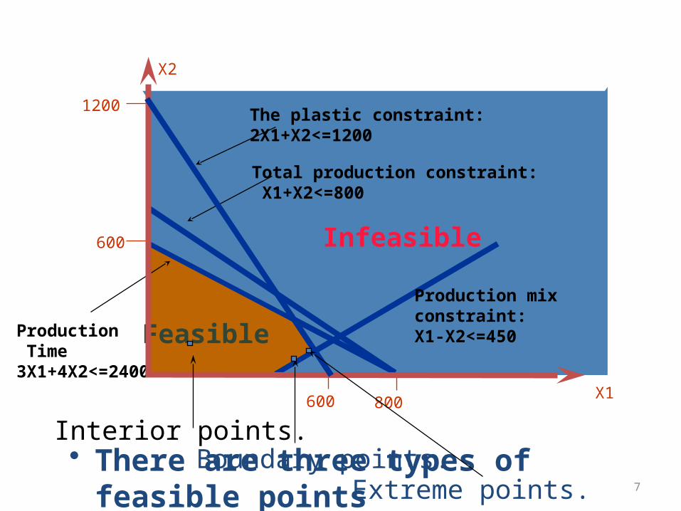
Max 8X1 + 5X2 (Weekly profit)subject to2X1 + 1X2 < = 1200 (Plastic)3X1 + 4X2 < = 2400 (Production Time) X1 + X2 < = 800 (Total production) X1 - X2 < = 450 (Mix) Xj> = 0, j = 1,2 (Nonnegativity)

7

1200

600

The Plastic constraint

Feasible

The plastic constraint: 2X1+X2<=1200

X2

Infeasible

Production Time3X1+4X2<=2400

Total production constraint: X1+X2<=800

600

800

Production mix constraint:X1-X2<=450

• There are three types of feasible points

Interior points.Boundary points.

Extreme points.

X1

8

Recall the fe

asible Region

600

800

1200

400 600 800

X2

X1

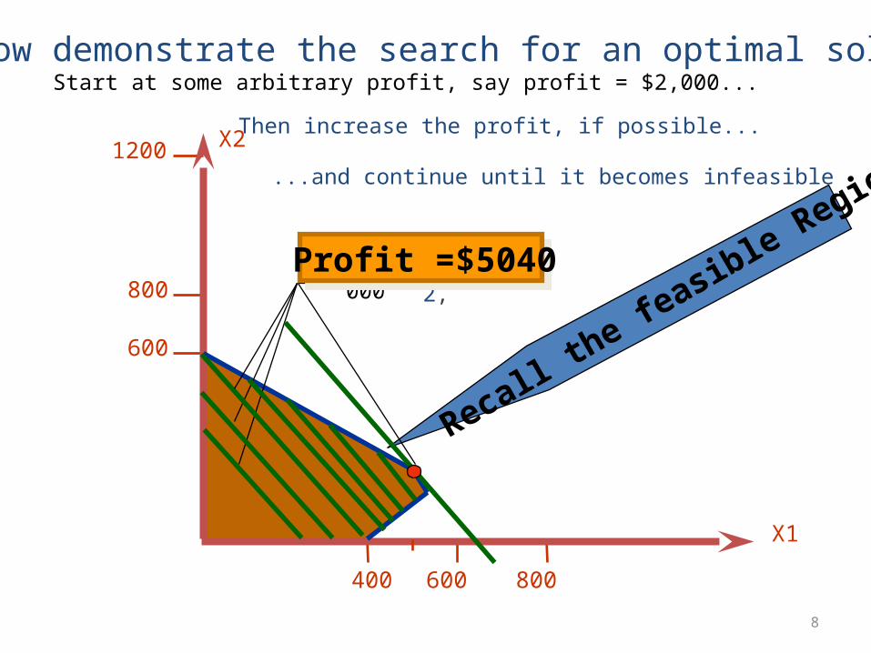
We now demonstrate the search for an optimal solution Start at some arbitrary profit, say profit = $2,000...

Profit = $ 000 2,

Then increase the profit, if possible...

3,4,

...and continue until it becomes infeasible

Profit =$5040

9

600

800

1200

400 600 800

X2

X1

Let’s take a closer look at the optimal point

FeasibleregionFeasibleregion

Infeasible

10

Summary of the optimal solution

Space Rays = 480 dozens Zappers = 240 dozens Profit = $5040

– This solution utilizes all the plastic and all the

production hours.

– Total production is only 720 (not 800).

– Space Rays production exceeds Zapper by only 240

dozens (not 450).

Chapter 3:Linear ProgrammingSensitivity Analysis

Sensitivity AnalysisWhat if there is uncertainly about one or more

values in the LP model?1. Raw material changes,2. Product demand changes, 3. Stock priceSensitivity analysis allows a manager to ask

certain hypothetical questions about the problem, such as:

How much more profit could be earned if 10 more hours of labour were available?

Which of the coefficient in model is more critical?

Sensitivity Analysis

Sensitivity analysis allows us to determine how “sensitive” the optimal solution is to changes in data values.

Is the optimal solution sensitive to changes in input parameters?

This includes analyzing changes in:1. An Objective Function Coefficient (OFC)2. A Right Hand Side (RHS) value of a constraint

Limit of Range of optimality

• Max Ax + BY• Keeping x, Y same how the object function

behaves if A, B are changed.• The optimal solution will remain unchanged as

long as An objective function coefficient lies within its range of optimality There are no changes in any other input parameters

• If the OFC changes beyond that range a new corner point becomes optimal.

• Generally, the limits of a range of optimality are found by changing the slope of the objective function line within the limits of the slopes of the binding constraint lines.

• Binding constraint • Are the constraints that restrict the feasible

region

Graphical Sensitivity Analysis

We can use the graph of an LP to see what happens when:

1. An OFC changes, or 2. A RHS changes

Recall the Flair Furniture problem

2x1 + 3x2 < 19

x1 + x2 < 8Max 5x1 + 7x2Max 5x1 + 7x2

x1 < 6

Optimal solution: x1 = 5, x2 = 3

Example 1:

Max 5x1 + 7x2

s.t. x1 6

2x1 + 3x2 < 19

x1 + x2 < 8

x1 > 0 and x2 > 0

Feasibleregion

Sensitivity to Coefficients

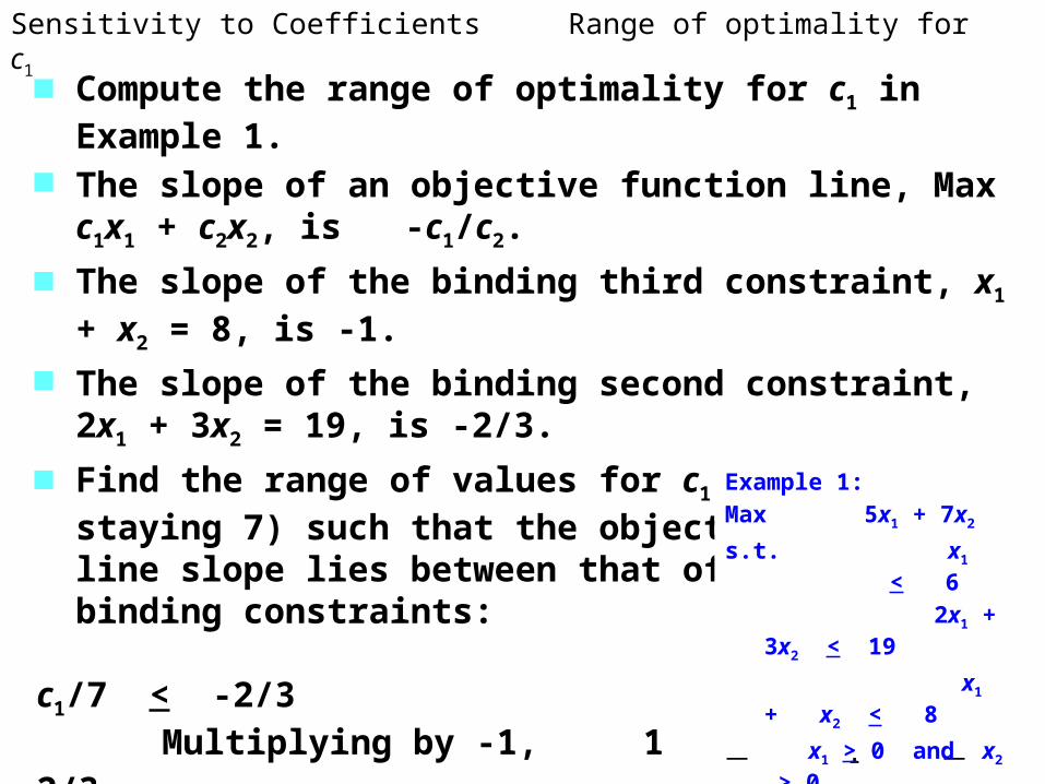
Compute the range of optimality for c1 in Example 1.

The slope of an objective function line, Max c1x1 + c2x2, is -c1/c2. The slope of the binding third constraint, x1 + x2 = 8, is -

1. The slope of the binding second constraint, 2x1 + 3x2 =

19, is -2/3. Find the range of values for c1 (with c2 staying 7) such

that the objective-function line slope lies between that of the two binding constraints:

-1 < -c1/7 < -2/3 Multiplying by -1, 1 > c1/7 > 2/3 Multiplying by 7, 7 > c1 > 14/3

Sensitivity to Coefficients Range of optimality for c1

Example 1:

Max 5x1 + 7x2

s.t. x1 < 6

2x1 + 3x2 < 19

x1 + x2 < 8

x1 > 0 and x2 > 0

Sensitivity to Coefficients Range of optimality for c2

Example 1:

Max 5x1 + 7x2

s.t. x1 < 6

2x1 + 3x2 < 19

x1 + x2 < 8

x1 > 0 and x2 > 0

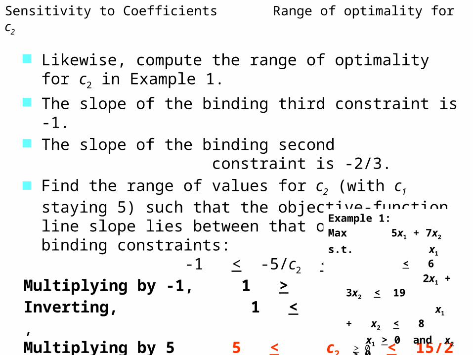
Likewise, compute the range of optimality for c2 in Example 1.

The slope of the binding third constraint is -1. The slope of the binding second

constraint is -2/3. Find the range of values for c2 (with c1 staying 5) such that

the objective-function line slope lies between that of the two binding constraints:

-1 < -5/c2 < -2/3Multiplying by -1, 1 > 5/c2 > 2/3Inverting, 1 < c2/5 < 3/2, Multiplying by 5 5 < c2 < 15/2

Example 1:

Max 5x1 + 7x2

s.t. x1 < 6

2x1 + 3x2 < 19

x1 + x2 < 8

x1 > 0 and x2 > 0

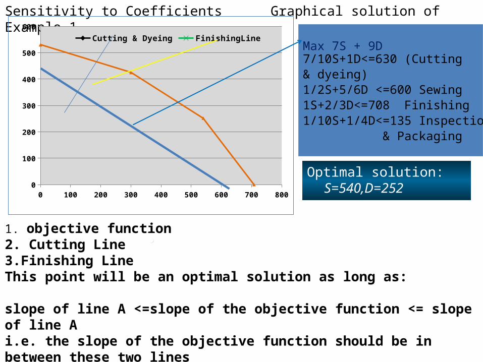
Optimal solution: S=540,D=252

Max 7S + 9D7/10S+1D<=630 (Cutting & dyeing)1/2S+5/6D <=600 Sewing1S+2/3D<=708 Finishing1/10S+1/4D<=135 Inspection

& Packaging

Sensitivity to Coefficients Graphical solution of Example 1

0 100 200 300 400 500 600 700 8000

100

200

300

400

500

600

Cutting & Dyeing FinishingLine

1. objective function2. Cutting Line3.Finishing LineThis point will be an optimal solution as long as:

slope of line A <=slope of the objective function <= slope of line Ai.e. the slope of the objective function should be in between these two lines

• 7/10S+D=630 (C&D)• D=-7/10S+630• S+2/3D=708 (Finishing)• D=-3/2S+1062• -3/2<=slope of objective function <=-7/10• -3/2<=-Cs/Cd<=-7/10• if we put profit contribution of delux bag same i.e 9• -3/2<=-Cs/9<=-7/10• Cs>=3*9/2• Cs>=27/2 • Cs>=13.5• Cs>=63/10• Cs>=6.3

• 6.3 <=Cs<=13.5 (limits for Cs with same optimal solution)

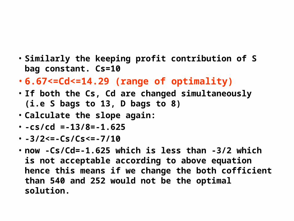
• Similarly the keeping profit contribution of S bag constant. Cs=10

• 6.67<=Cd<=14.29 (range of optimality)• If both the Cs, Cd are changed simultaneously (i.e S bags to 13,

D bags to 8)• Calculate the slope again:• -cs/cd =-13/8=-1.625• -3/2<=-Cs/Cs<=-7/10• now -Cs/Cd=-1.625 which is less than -3/2 which is not

acceptable according to above equation hence this means if we change the both cofficient than 540 and 252 would not be the optimal solution.

• Multiple changes

– The range of optimality is valid only when a single

objective function coefficients changes.

– When more than one variable changes we turn to

the

100% rule

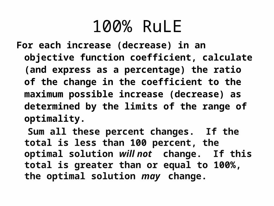
100% RuLEFor each increase (decrease) in an objective

function coefficient, calculate (and express as a percentage) the ratio of the change in the coefficient to the maximum possible increase (decrease) as determined by the limits of the range of optimality.

Sum all these percent changes. If the total is less than 100 percent, the optimal solution will not change. If this total is greater than or equal to 100%, the optimal solution may change.

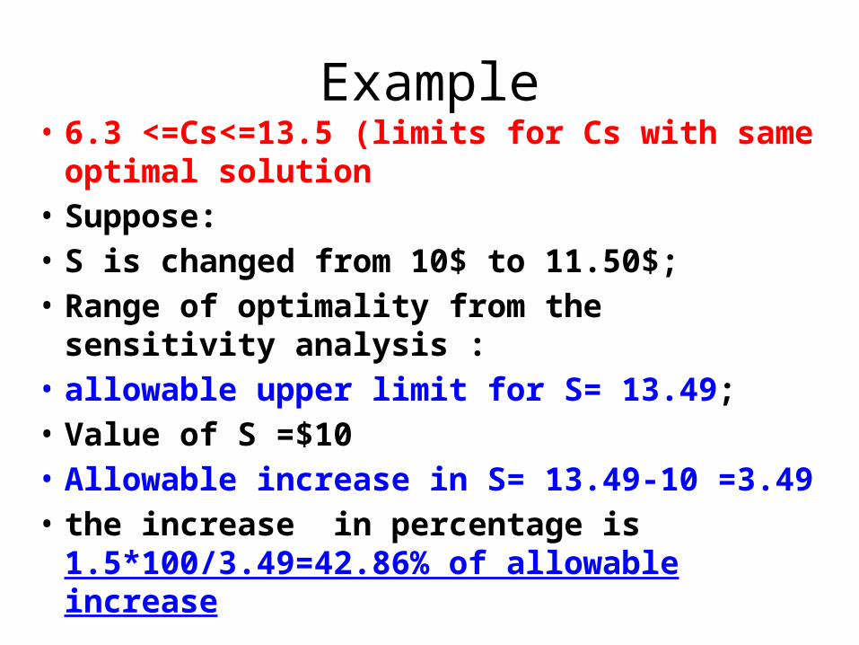
Example• 6.3 <=Cs<=13.5 (limits for Cs with same optimal

solution• Suppose:• S is changed from 10$ to 11.50$; • Range of optimality from the sensitivity analysis :• allowable upper limit for S= 13.49; • Value of S =$10 • Allowable increase in S= 13.49-10 =3.49• the increase in percentage is

1.5*100/3.49=42.86% of allowable increase

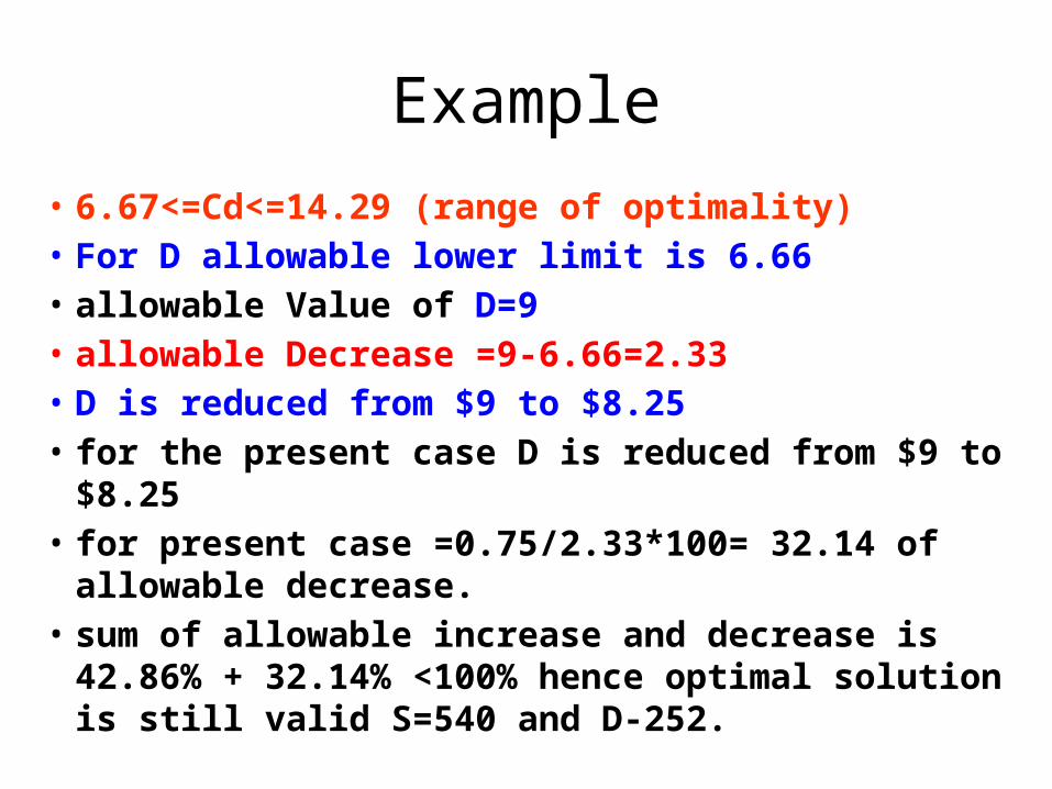
Example• 6.67<=Cd<=14.29 (range of optimality)• For D allowable lower limit is 6.66• allowable Value of D=9• allowable Decrease =9-6.66=2.33• D is reduced from $9 to $8.25• for the present case D is reduced from $9 to $8.25• for present case =0.75/2.33*100= 32.14 of allowable

decrease.• sum of allowable increase and decrease is 42.86% +

32.14% <100% hence optimal solution is still valid S=540 and D-252.

Effect of change of the right hand side of the constraint.

• Any change in a right hand side of a binding constraint will change the optimal solution.

• Any change in a right-hand side of a nonbinding constraint that is less than its slack or surplus, will cause no change in the optimal solution.

Keeping all other factors the same, how much would the optimal value of the objective function (for example, the profit) change if the right-hand side of a constraint changed by one unit?

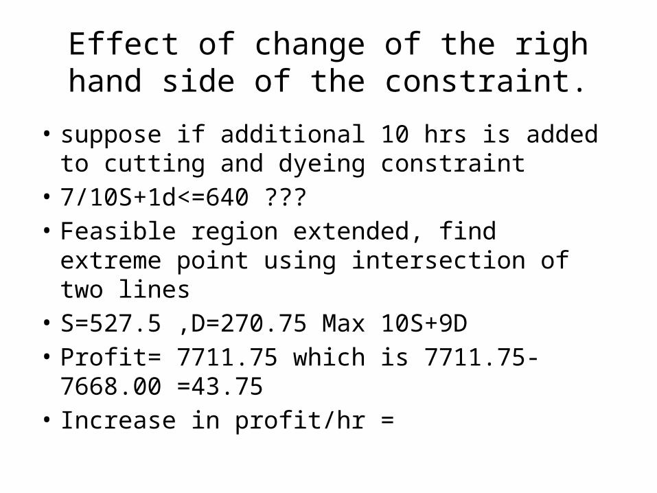
Effect of change of the righ hand side of the constraint.

• suppose if additional 10 hrs is added to cutting and dyeing constraint

• 7/10S+1d<=640 ???• Feasible region extended, find extreme point

using intersection of two lines• S=527.5 ,D=270.75 Max 10S+9D• Profit= 7711.75 which is 7711.75-7668.00

=43.75 • Increase in profit/hr =

Dual Price

• It is the improvement in the optimal solution per unit increase in the RHS of constraint

• If dual price is negative this means value of objective function will not improved rather it would get worse ,if value at rhs of the constrain is increased by 1 unit . for minimization problem it means cost will increase by 10.

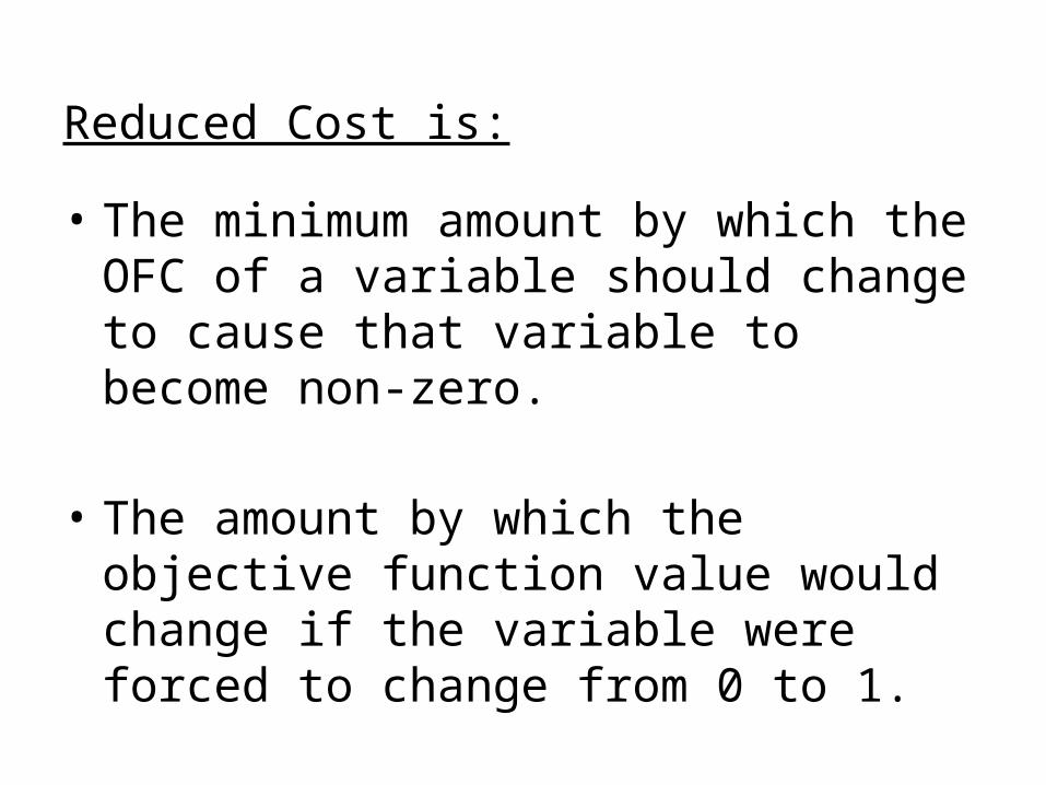
Reduced Cost is:

• The minimum amount by which the OFC of a variable should change to cause that variable to become non-zero.

• The amount by which the objective function value would change if the variable were forced to change from 0 to 1.

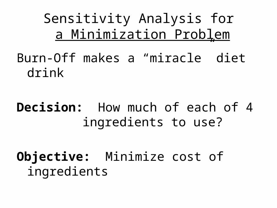
Sensitivity Analysis for a Minimization Problem

Burn-Off makes a “miracle” diet drink

Decision: How much of each of 4 ingredients to use?

Objective: Minimize cost of ingredients

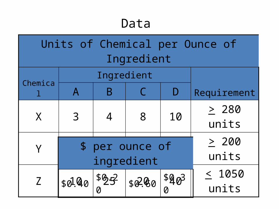
Data Units of Chemical per Ounce of Ingredient

Chemical

Ingredient

RequirementA B C DX 3 4 8 10 > 280 units

Y 5 3 6 6 > 200 units

Z 10 25 20 40 < 1050 units

$ per ounce of ingredient

$0.40 $0.20 $0.60 $0.30

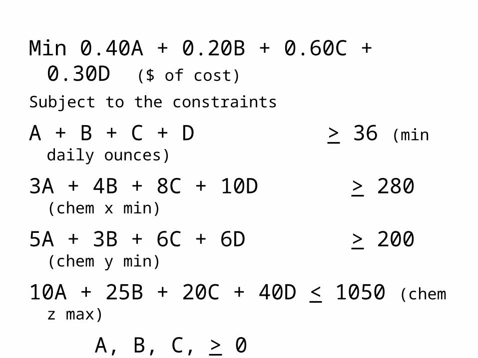
Min 0.40A + 0.20B + 0.60C + 0.30D ($ of cost)

Subject to the constraints

A + B + C + D > 36 (min daily ounces)

3A + 4B + 8C + 10D > 280 (chem x min)

5A + 3B + 6C + 6D > 200 (chem y min)

10A + 25B + 20C + 40D < 1050 (chem z max)

A, B, C, > 0