Transportation Research Part C 56 (2015) 177–194

Contents lists available at ScienceDirect

Transportation Research Part C

journal homepage: www.elsevier .com/locate / t rc

Vehicular Ad-Hoc Networks sampling protocols for trafficmonitoring and incident detection in Intelligent TransportationSystems

http://dx.doi.org/10.1016/j.trc.2015.03.0410968-090X/� 2015 Elsevier Ltd. All rights reserved.

⇑ Corresponding author.E-mail addresses: andrea.baiocchi@uniroma1.it (A. Baiocchi), francesca.cuomo@uniroma1.it (F. Cuomo), mario.defelice@uniroma1.it (M. D

gaetano.fusco@uniroma1.it (G. Fusco).

Andrea Baiocchi a,⇑, Francesca Cuomo a, Mario De Felice a, Gaetano Fusco b

a Dept. of Information Engineering, Electronics and Telecommunications (DIET), Sapienza University of Rome, Via Eudossiana 18, 00184 Rome, Italyb Dept. of Civil, Architectural and Environmental Engineering, (DICEA), Sapienza University of Rome, Via Eudossiana 18, 00184 Rome, Italy

a r t i c l e i n f o a b s t r a c t

Article history:Received 25 November 2014Received in revised form 12 March 2015Accepted 26 March 2015Available online 19 April 2015

Keywords:Vehicular traffic monitoringVANETIncident detectionDistributed algorithmsFCD collectionMulti-hop communications

Vehicular Ad-Hoc Networks (VANETs) are an emerging technology soon to be brought toeveryday life. Many Intelligent Transport Systems (ITS) services that are nowadays per-formed with expensive infrastructure, like reliable traffic monitoring and car accidentdetection, can be enhanced and even entirely provided through this technology. In thispaper, we propose and assess how to use VANETs for collecting vehicular traffic measure-ments. We provide two VANET sampling protocols, named SAME and TOME, and we designand implement an application for one of them, to perform real time incident detection. Theproposed framework is validated through simulations of both vehicular micro-mobilityand communications on the 68 km highway that surrounds Rome, Italy. Vehicular trafficis generated based on a large real GPS traces set measured on the same highway, involvingabout ten thousand vehicles over many days. We show that the sampling monitoring pro-tocol, SAME, collects data in few seconds with relative errors less than 10%, whereas theexhaustive protocol TOME allows almost fully accurate estimates within few tens of sec-onds. We also investigate the effect of a limited deployment of the VANET technology onboard of vehicles. Both traffic monitoring and incident detection are shown to still be fea-sible with just 50% of equipped vehicles.

� 2015 Elsevier Ltd. All rights reserved.

1. Introduction

Intelligent Transportation Systems (ITSs) integrate Information and Communications Systems (ICT) with transportationengineering methods to get an improved knowledge of current and future states of the transportation system and, possibly,to react to unexpected perturbations in order to keep the system near a desired state of safety, efficiency and comfort. ITSsenhance efficiency and effectiveness of the interactions among different components of the transport system (vehicles, road,drivers) thanks to a set of sensors that monitor the near and the far environment, and a set of actuators that put in practicepredetermined control rules.

Vehicular Ad-Hoc Networks (VANETs) allow Dedicated Short Range Communications (DSRC) of vehicles in the 5.9 GHzband, through the IEEE 802.11p standard. They support ITS with both Vehicle-to-Vehicle (V2V) and Vehicle-to-Infrastructure (V2I) communications for applications in both near and far environment; in such a way, VANETs are a

e Felice),

178 A. Baiocchi et al. / Transportation Research Part C 56 (2015) 177–194

technology that enables a unified framework for integrating traditional ITS applications, Advanced Driver Assistance Systems(ADAS), Advanced Traveller Information Systems (ATIS), and Advanced Traffic Management Systems (ATMS).

Applications of V2V/V2I communications to ATIS and ATMS provide these systems with a monitoring subsystem thatexploits equipped vehicles as probes in the traffic stream and, at the same time, with a communication system that allowsvehicles exchanging information with each other regarding current traffic speed or any other useful message on traffic con-ditions. ATIS and ATMS can be effectively integrated in order to have a unique platform that controls regulation devices suchas traffic signals and provides users with updated proactive information in a consistent way. Not only traffic monitoring andcommunication tasks are transferred to vehicle communication devices; also a significant part of data processing can be dis-tributed and conveyed to the vehicle communication network, since on-board devices can apply transmission protocols thatprocess data exchanged between vehicles without requiring transmission and processing of data by a traffic control center.

Effectiveness of VANET applications on ATIS/ATMS is significantly affected by the penetration rate of equipped vehicles,which impacts primarily on the communication network reliability. It is worth noticing that, even if information transmis-sion can be ensured, penetration rate determines the sample of vehicles tracked and then the accuracy of traffic state esti-mates, thus affecting the reliability and effectiveness of the system.

In this work we look at a perspective where the majority of vehicles are equipped with standardized VANET On BoardUnits (OBU) and we explore the potential of VANETs in the collection of Floating Car Data (FCD) over urban highways.Specifically, we aim at assessing the effectiveness of FCD collection through VANET multi-hop communications in orderto minimize the required fixed infra-structure. We made a preliminary investigation of this problem in De Felice et al.(2014). Here we provide a more formal description of the VANET protocols and an in-depth performance evaluation of anincident detection algorithm on top of the VANET based monitoring system. The algorithm is shown to be quite effective,in spite of the simplicity of the VANET system and of the light load it imposes on the VANET (0.08 kbps for the sampledFCD collection and 40–50 kbps for the exhaustive collection).

We test the algorithm by setting up incident scenarios on an urban highway ring about 70 km long, around Rome, Italy.Micro-mobility is simulated with SUMO (e.g., see Behrisch et al. (2011)) and the communication process by means of NS2(e.g., see Fall and Varadhan (2000)). Vehicular traffic generation is tuned by means of massive GPS real data collected fromvehicles monitored on the same highway. We investigate the impact of the penetration rate of VANET equipment on trafficmonitoring and incident detection capabilities. Our approach still works when not all the vehicles are equipped with DSRCdevices.

To sum up, the major contributions of this work are: (i) definition of two practical, lightweight protocols for vehiculartraffic monitoring based on VANET; (ii) detailed, integrated simulations of micro-mobility and communications, trainedby real vehicular data; (iii) definition and evaluation of a real time incident detection algorithm exploiting the traffic datacollected by the VANET based protocol.

The rest of the paper is so organized. The related literature is reviewed in Section 2. The VANET data collection protocolsare presented in Section 3. Section 4 outlines the simulation scenario used to test the protocol performance, based on a realhighway and driven by vehicular traffic generated from real data. A performance evaluation analysis is presented inSection 5. Conclusions are drawn in Section 6.

2. Related work

In the last years, a broad literature arose concerning VANET applications to different ITS subsystems, ranging from ADAS(specifically, cooperative collision warning), to ATMS (as far as virtual traffic lights, traffic monitoring, incident detection)and ATIS (regarding advanced speed control, route guidance). Traditional traffic monitoring systems are based on fixed sen-sors, like inductive loops or video image processors, which detect traffic state variables, such as occupancy, flow and some-times speed, and process the collected data to detect possible incidents or predict future traffic conditions in the short term.

A comprehensive overview of the vast literature on this field is out of the scope of this paper. The interested reader canrefer to Vlahogianni et al. (2014) for an updated critical review of the recent literature. We just focus here on incident detec-tion algorithms, which provide a partial but significant example of diagnostic models.

Incident detection algorithms developed in the 70s, like California of Payne and Tignor (1978), were based on occupancymeasures at fixed road sections and tried to recognize anomalous conditions by comparing upstream and downstreamtraffic density measures; that is, by observing the effects of the incident on traffic flow. Statistical algorithms detect sig-nificant differences between observed data and traffic characteristics predicted by prior probabilities, as done byDudek et al. (1974), or by time-series and filtering analysis, as in Ahmed and Cook (1982), Stephanedes and Chassiakos(1993).

McMaster algorithm applied the Catastrophe theory to recognize an abrupt interruption of the regular pattern in theflow-speed-occupancy space (Persaud et al., 1990). Then, several different methods were introduced that apply artificialintelligence techniques, including neural networks (Stephanedes and Liu, 1995; Adeli and Samant, 2000), fuzzy logic (Linand Chang, 1998), and a combination of these two techniques, as in Hsiao et al. (1994), Ishak and Al-Deek (1998).

The performances of the aforementioned algorithms depend on the balance of the thresholds chosen for incident identi-fication. If thresholds that provide false alarm lower than 2% are chosen, the mean time to detect an incident ranges fromabout 1 min to 6–8 min (Mahmassani et al., 1998).

A. Baiocchi et al. / Transportation Research Part C 56 (2015) 177–194 179

Recently, Li et al. (2014) introduced an enhanced statistical metric into traffic parameters used to detect an incident,namely the coefficient of variation of speed at the upstream detector and the correlation coefficient of speeds of two adjacentdetectors. Wang et al. (2013) developed a hybrid method that applies a machine learning classifier to detect incidents bycomparing real-time traffic and forecasts of the normal traffic for the current time point based on prior normal traffic.

Several studies have shown that vehicle-generated data can provide reliable estimates of traffic conditions, includingidentification of incidents and congestion (Sermons and Koppelman, 1996; Long Cheu et al., 2002), and origin–destinationmatrix estimation, as done in Barcelò et al. (2013). An application level framework was defined in Borsetti et al. (2011) todisseminate data and collect road-sensor information through floating vehicles. Dia and Thomas (2011) devised a neural net-work algorithm that uses a fusion of data from loop detectors and probe vehicles identified by fixed devices. Bigger advan-tages can be obtained, however, by collecting data directly from floating cars; that is, vehicles that move on the roadnetwork. Geisler et al. (2012) presented an evaluation framework for traffic information systems based on data streams frommobile phones and applied it in two case studies, namely queue-end detection and traffic state estimation, simulated in theidealistic case of two highways links of 5 km length.

In the last years, several authors studied applications of VANET inter-vehicle communications to monitor traffic andrecognize incident conditions by using probe vehicle information. Yin et al. (2013) investigated connectivity issues and pro-posed an analytical model for the vehicle connectivity on two parallel roadways, assuming general distributions for vehicleheadways. However, most authors tested the effectiveness of these applications through simulation models. Sommer et al.(2011) developed a hybrid bidirectional simulation environment called VEINS, composed of the network simulator OMNeT++and the road traffic simulator SUMO. They devised a simple incident detection method based on alerts sent by vehicles withspeed of zero and tested it in several incident scenarios.

Abuelela et al. (2009) proposed a Bayesian approach to traffic incident detection based on the counts of lane changesrecorded in each road segment. In that architecture, vehicles are equipped with high accuracy GPS, record their positionsand transmit any lane change to roadside units, which store time instants and locations of all the lane changes occurredon the road segment associated with them. Khorashadi et al. (2011) envisioned a decentralized system that exploits coopera-tive potentials of a distributed communication system among vehicles and applies a two-phase anomaly detection. In thefirst phase, each vehicle independently checks a set of conditions for different densities, lane changes and average speedbetween consecutive road sections. In a second phase, a voting mechanism among vehicles is applied to verify the existenceof an obstruction point on the road.

Terroso-Sáenz et al. (2012) introduced an event driven architecture to monitor traffic and detect incidents combining themessages exchanged between VANET equipped vehicles that monitor individual speed profiles and combining them withother sources of information. A set of event processing agents checks for single slow vehicles and external events, processessuch information to individuate slow vehicle groups and detects congestion occurrence through a fuzzy classifier that takesin input traffic speed and density and classifies them depending on weather conditions.

Ma et al. (2009) envisioned a real-time travel incident detection method based on two Artificial Intelligence paradigms(namely, Artificial Neural Networks and Support Vector Machine) that exploits vehicle-infrastructure integration and pro-cesses individual speed profiles and lane changes to classify possible incident conditions. They analyzed their methodthrough a simulation experiment on a small freeway network, which showed that the proposed framework outperforms tra-ditional incident detection methods based on point traffic measures like California algorithm. Bauza and Gozálvez (2013)devised a cooperative traffic congestion detection method in which every vehicle continuously monitors the road traffic con-ditions through messages received by neighboring vehicles, computes local values of traffic density and estimates through afuzzy model the corresponding level of congestion. When such level exceeds a given threshold, vehicles perform a coopera-tive procedure based on multi-hop communication to achieve a consensus decision. A specific procedure identifies the vehi-cle close to the front end of the queue and allows estimating the length of the traffic jam.

Another important contribution was provided by Santamaria et al. (2014), where the authors monitor the traffic with aninteresting approach for urban scenarios: they implement collision detection and smart traffic management applicationswith a centralized and strongly infrastructured approach.

In our approach, we do not need any overhead packet for the network organization and control or consensus like in Bauzaand Gozálvez (2013); we also do not rely on local voting processes, that may be local sub-optima, like Khorashadi et al.(2011): our mechanism is auto-referenced and lightweight, so we do not need further external data (like Terroso-Sáenzet al., 2012).

Processing large amount of data to describe speed profiles or individual lane changes is not required, like most of theabovementioned papers; however, it aggregates individual speed measures to estimate average traffic conditions andexploits the number of vehicles with zero speed as a variable that reveals possible incident occurrence.

Above all, the distinctive point of our approach is its capability to function even without a fully collaborative environment(not having all the vehicles equipped with the DSRC technology is a possibility that is considered in the study presented inthis paper), which is not considered in most of the other works. Moreover, most of the other studies assume a significantmonitoring infrastructure deployed on roads; we show that a single fixed Road Side Unit (RSU) is enough to support the pro-posed VANET protocol scheme over a 70 km long highway. This highlights the value of exploiting the communication equip-ment that will be deployed on board vehicles under the push of safety constraints in the next several years.

Furthermore, although we rely on GPS, we can tolerate significant system imprecision, that may be due to the presence ofbuildings, flyovers, tunnels and other obstacles that invalidate the system precision, since we do not need to be lane-aware

180 A. Baiocchi et al. / Transportation Research Part C 56 (2015) 177–194

or highly precise: the GPS just has to put a sample in a road segment which maybe up to 3 km long. This is a very robustassumption, which makes our study much closer to real conditions that may happen on a real highway.

3. The VANET monitoring system

Floating Car Data (FCD) are generated by on board vehicle equipment and can be collected by having vehicles communi-cating with a fixed infrastructure via, e.g., cellular network or VANET. The latter lends itself to sampling collection with mini-mal infrastructure deployment, especially in high density traffic, by exploiting multi-hop message passing among vehicles.

In the following we assume that FCD messages must be collected by one RSU in charge of monitoring a given road system.The RSU radio coverage is limited to a fraction of the area to be monitored. As a matter of example, transmission ranges are inthe order of several hundreds meters, while the road system used as a reference in the evaluation presented in Section 5consists of a ring highway 68 km long. Therefore FCD messages are delivered to the RSU by hopping through intermediatecommunication nodes, inside OBU equipped vehicles.

The key idea of the FCD collection protocol presented here is to have one RSU trigger the data collection by sending an‘‘invite’’ message, with a unique sequence number k, that hops through selected vehicles, acting as forwarding nodes, andgets back to the original RSU (or arrives at another designated RSU) with a list of FCD appended by the intermediate forward-ing vehicles.

Let us consider a generic single hop, i.e., a communication between two equipped vehicles within radio transmissionrange of each other. ehicle A transmits the FCD collection message with sequence number k (having appended its own data).All vehicles within range of A receive the message and set a timer whose duration is a decreasing function of the distancebetween A and the receiving vehicle. Thus, the timer of the furthest away vehicle from A will expire first and that vehiclewill forward the message with sequence number k (having appended in turn its own FCD). A critical issue is to avoid thebroadcast storm problem, highlighted by Ni et al. (1999), while insisting on distributed algorithms for message generationand delivery. To avoid loading the radio interface with too many messages, an inhibition rule is defined, i.e., a vehicle willabort the forwarding action scheduled for the first copy of a message upon reception of a second copy of the message withthe same sequence number.

The general idea outlined above is developed in detail in the two ensuing subsections. Two protocols are defined. A firstone, SAME (SAmpled Measurement Estimation, Section 3.1), accomplishes sampling of vehicles and collects one FCD sampleat each hop, i.e., every some hundred meters along the monitored road. The second protocol, TOME (Timer-based OrderedMeasurement Estimation, Section 3.2), is designed for extensive FCD collection and aims at providing the monitoring pointwith averaged measures, referred to sectors of the monitored road. This implies message passing among vehicles and in-net-work processing of collected data.

3.1. Monitoring by sampling vehicles – SAME

Let us consider two RSUs located along a road span, RSUa and RSUb. RSUa originates a stream of messages, issuing oneMeasurement Collection (MC) message every time interval TRSU . The MC message is passed over from vehicle to vehicle untilit reaches RSUb, that is the final sink of the collected measurements.

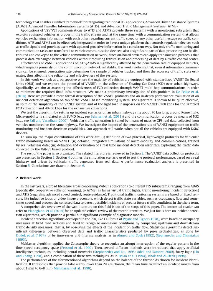
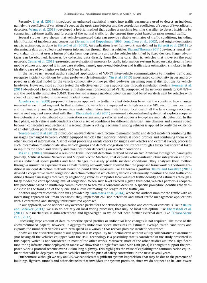
The SAME message structure is shown in Fig. 1, the list of symbols and acronyms used to refer to the fields of the MC

message is provided in Table 1 (gray rows are specific of TOME, see Section 3.2).The SAME MC comprises a sequence number and a hop count, both initialized by the RSUa. The sequence number is incre-

mented only by RSUa, for each new MC message issued. The hop count is set to 0 by RSUa and it is incremented by eachintermediate forwarding node. The SAME MC contains also a list L where FCDs of the sampled vehicles will be appended.The list is initially empty and the relevant length filed is set to 0 by RSUa.

At each hop, the node that sends the message adds a record to MC, denoted as Vehicle Block VB, with its own data: vehi-cle ID, timestamp, coordinates of the vehicle, direction of motion and velocity.1 Coordinates and timestamp can be obtainedfrom a GPS receiver on board the vehicle. Besides adding its own FCD record, each intermediate forwarding node moves the VB

it finds at the end of the received message to the list L, by appending it at the end of the list. The list length field is then incre-mented by 1.

The size M of the list L eventually delivered to RSUb depends on the number of intermediate sampled vehicles, that is thenumber of vehicles forwarding the message from RSUa up to RSUb. The list size M is related to the average hop length and tothe length of the monitored road span. A fast polling is possible, since each forwarding hop takes a time in the order of mil-liseconds and typical hop lengths can be several hundred meters. The traveling speed of the monitoring messages can bethus in the order of tens of km/s, three orders of magnitude more than vehicle speed.

Measurements are collected at the RSUb and can be used to track the traffic average speed and density in each sector ofthe monitored road span. Polling is repeated every TRSU seconds. TRSU is to be chosen so as to detect vehicular traffic varia-tions quickly and reliably (that entails collecting tens of samples over a time scale comparable with that of vehicle motion,namely tens of seconds) and to keep the collecting protocol performance near to optimal by avoiding communication

1 These last two fields are left at 0 by the originating RSU.

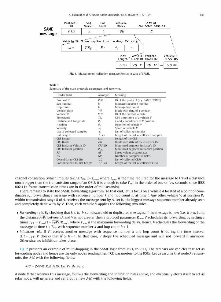
Fig. 1. Measurement collection message format in case of SAME.

Table 1Summary of the main protocols parameters and acronyms.

A. Baiocchi et al. / Transportation Research Part C 56 (2015) 177–194 181

channel congestion (which implies taking TRSU � sprop, where sprop is the time required for the message to travel a distancemuch bigger than the transmission range of an OBU; it is enough to take TRSU in the order of one or few seconds, since IEEE802.11p frame transmission times are in the order of milliseconds).

There remains to state the SAME forwarding algorithm. To that end, let us focus on a vehicle A located at a point of coor-dinates PA, forwarding a message with sequence number k and hop count h, at time t. Any other vehicle V, at position PV

within transmission range R of A, receives the message sent by A. Let kV the biggest message sequence number already seenand completely dealt with by V. Then, each vehicle V applies the following two rules:

� Forwarding rule. By checking that k 6 kV ;V can discard old or duplicated messages. If the message is new (i.e., k > kV ) andthe distance PV PA between A and V is not greater then a protocol parameter Rmax;V schedules its forwarding by setting atimer TV ;k ¼ Tmaxð1� PV PA=RmaxÞ, where Tmax is the maximum forwarding delay. Hence, V schedules the forwarding of themessage at time t þ TV ;k with sequence number k and hop count hþ 1.� Inhibition rule. If V receives another message with sequence number k and hop count h0 during the time intervalðt; t þ TV ;k�;V checks that h0 P hþ 1. In that case, V drops the scheduled message and will not forward it anymore.Otherwise, no inhibition takes place.

Fig. 2 presents an example of multi-hopping in the SAME logic from RSUa to RSUb. The red cars are vehicles that act asforwarding nodes and hence are the only nodes sending their FCD parameters to the RSUb. Let us assume that node A retrans-mits the MC with the following fields:

MC ¼ ½SAME; k;h;A:ID; TSA; PA; d̂A;vA;L�

A node B that receives this message, follows the forwarding and inhibition rules above, and eventually elects itself to act asrelay node, will generate and send out a new MC with the following fields:

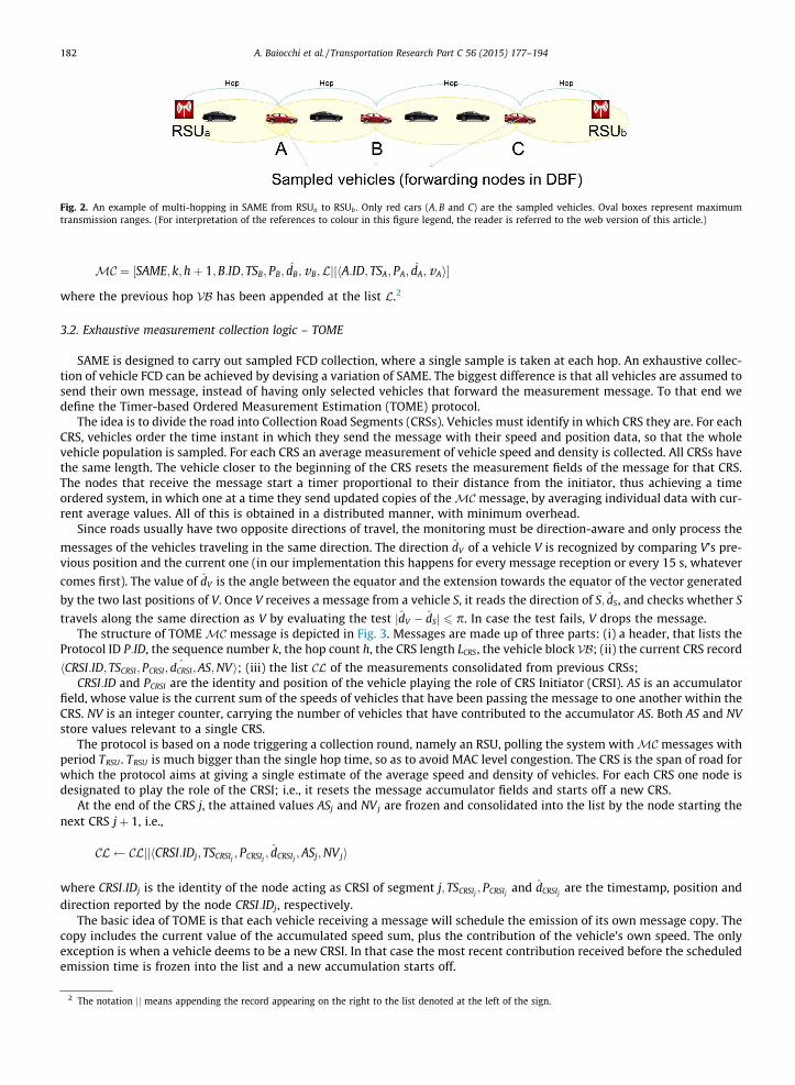
Fig. 2. An example of multi-hopping in SAME from RSUa to RSUb . Only red cars (A;B and C) are the sampled vehicles. Oval boxes represent maximumtransmission ranges. (For interpretation of the references to colour in this figure legend, the reader is referred to the web version of this article.)

2 The

182 A. Baiocchi et al. / Transportation Research Part C 56 (2015) 177–194

MC ¼ ½SAME; k; hþ 1;B:ID; TSB; PB; d̂B; vB;LjjhA:ID; TSA; PA; d̂A; vAi�

where the previous hop VB has been appended at the list L.2

3.2. Exhaustive measurement collection logic – TOME

SAME is designed to carry out sampled FCD collection, where a single sample is taken at each hop. An exhaustive collec-tion of vehicle FCD can be achieved by devising a variation of SAME. The biggest difference is that all vehicles are assumed tosend their own message, instead of having only selected vehicles that forward the measurement message. To that end wedefine the Timer-based Ordered Measurement Estimation (TOME) protocol.

The idea is to divide the road into Collection Road Segments (CRSs). Vehicles must identify in which CRS they are. For eachCRS, vehicles order the time instant in which they send the message with their speed and position data, so that the wholevehicle population is sampled. For each CRS an average measurement of vehicle speed and density is collected. All CRSs havethe same length. The vehicle closer to the beginning of the CRS resets the measurement fields of the message for that CRS.The nodes that receive the message start a timer proportional to their distance from the initiator, thus achieving a timeordered system, in which one at a time they send updated copies of the MC message, by averaging individual data with cur-rent average values. All of this is obtained in a distributed manner, with minimum overhead.

Since roads usually have two opposite directions of travel, the monitoring must be direction-aware and only process the

messages of the vehicles traveling in the same direction. The direction d̂V of a vehicle V is recognized by comparing V’s pre-vious position and the current one (in our implementation this happens for every message reception or every 15 s, whatever

comes first). The value of d̂V is the angle between the equator and the extension towards the equator of the vector generated

by the two last positions of V. Once V receives a message from a vehicle S, it reads the direction of S; d̂S, and checks whether S

travels along the same direction as V by evaluating the test jd̂V � d̂Sj 6 p. In case the test fails, V drops the message.The structure of TOME MC message is depicted in Fig. 3. Messages are made up of three parts: (i) a header, that lists the

Protocol ID P:ID, the sequence number k, the hop count h, the CRS length LCRS, the vehicle block VB; (ii) the current CRS record

hCRSI:ID; TSCRSI; PCRSI;^dCRSI;AS;NVi; (iii) the list CL of the measurements consolidated from previous CRSs;

CRSI:ID and PCRSI are the identity and position of the vehicle playing the role of CRS Initiator (CRSI). AS is an accumulatorfield, whose value is the current sum of the speeds of vehicles that have been passing the message to one another within theCRS. NV is an integer counter, carrying the number of vehicles that have contributed to the accumulator AS. Both AS and NVstore values relevant to a single CRS.

The protocol is based on a node triggering a collection round, namely an RSU, polling the system with MC messages withperiod TRSU . TRSU is much bigger than the single hop time, so as to avoid MAC level congestion. The CRS is the span of road forwhich the protocol aims at giving a single estimate of the average speed and density of vehicles. For each CRS one node isdesignated to play the role of the CRSI; i.e., it resets the message accumulator fields and starts off a new CRS.

At the end of the CRS j, the attained values ASj and NVj are frozen and consolidated into the list by the node starting thenext CRS jþ 1, i.e.,

CL CLjjhCRSI:IDj; TSCRSIj; PCRSIj

; d̂CRSIj;ASj;NVji

where CRSI:IDj is the identity of the node acting as CRSI of segment j; TSCRSIj; PCRSIj

and d̂CRSIjare the timestamp, position and

direction reported by the node CRSI:IDj, respectively.The basic idea of TOME is that each vehicle receiving a message will schedule the emission of its own message copy. The

copy includes the current value of the accumulated speed sum, plus the contribution of the vehicle’s own speed. The onlyexception is when a vehicle deems to be a new CRSI. In that case the most recent contribution received before the scheduledemission time is frozen into the list and a new accumulation starts off.

notation jj means appending the record appearing on the right to the list denoted at the left of the sign.

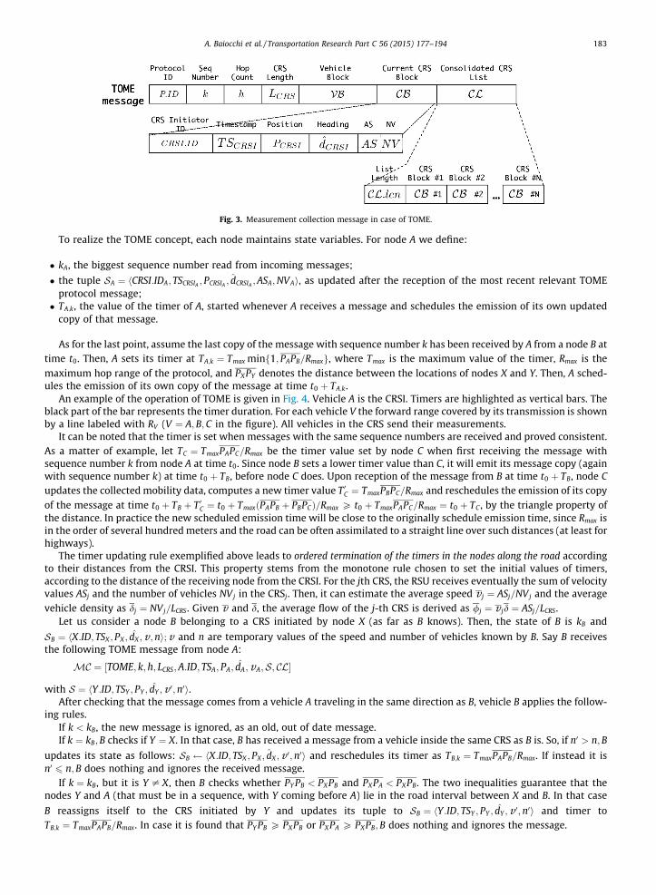
Fig. 3. Measurement collection message in case of TOME.

A. Baiocchi et al. / Transportation Research Part C 56 (2015) 177–194 183

To realize the TOME concept, each node maintains state variables. For node A we define:

� kA, the biggest sequence number read from incoming messages;

� the tuple SA ¼ hCRSI:IDA; TSCRSIA ; PCRSIA ; d̂CRSIA ;ASA;NVAi, as updated after the reception of the most recent relevant TOMEprotocol message;� TA;k, the value of the timer of A, started whenever A receives a message and schedules the emission of its own updated

copy of that message.

As for the last point, assume the last copy of the message with sequence number k has been received by A from a node B attime t0. Then, A sets its timer at TA;k ¼ Tmax minf1; PAPB=Rmaxg, where Tmax is the maximum value of the timer, Rmax is themaximum hop range of the protocol, and PXPY denotes the distance between the locations of nodes X and Y. Then, A sched-ules the emission of its own copy of the message at time t0 þ TA;k.

An example of the operation of TOME is given in Fig. 4. Vehicle A is the CRSI. Timers are highlighted as vertical bars. Theblack part of the bar represents the timer duration. For each vehicle V the forward range covered by its transmission is shownby a line labeled with RV (V ¼ A;B;C in the figure). All vehicles in the CRS send their measurements.

It can be noted that the timer is set when messages with the same sequence numbers are received and proved consistent.As a matter of example, let TC ¼ TmaxPAPC=Rmax be the timer value set by node C when first receiving the message withsequence number k from node A at time t0. Since node B sets a lower timer value than C, it will emit its message copy (againwith sequence number k) at time t0 þ TB, before node C does. Upon reception of the message from B at time t0 þ TB, node Cupdates the collected mobility data, computes a new timer value T 0C ¼ TmaxPBPC=Rmax and reschedules the emission of its copyof the message at time t0 þ TB þ T 0C ¼ t0 þ TmaxðPAPB þ PBPCÞ=Rmax P t0 þ TmaxPAPC=Rmax ¼ t0 þ TC , by the triangle property ofthe distance. In practice the new scheduled emission time will be close to the originally schedule emission time, since Rmax isin the order of several hundred meters and the road can be often assimilated to a straight line over such distances (at least forhighways).

The timer updating rule exemplified above leads to ordered termination of the timers in the nodes along the road accordingto their distances from the CRSI. This property stems from the monotone rule chosen to set the initial values of timers,according to the distance of the receiving node from the CRSI. For the jth CRS, the RSU receives eventually the sum of velocityvalues ASj and the number of vehicles NVj in the CRSj. Then, it can estimate the average speed v j ¼ ASj=NVj and the averagevehicle density as dj ¼ NVj=LCRS. Given v and d, the average flow of the j-th CRS is derived as /j ¼ v jd ¼ ASj=LCRS.

Let us consider a node B belonging to a CRS initiated by node X (as far as B knows). Then, the state of B is kB and

SB ¼ hX:ID; TSX ; PX ; d̂X ;v ;ni; v and n are temporary values of the speed and number of vehicles known by B. Say B receivesthe following TOME message from node A:

MC ¼ ½TOME; k;h; LCRS;A:ID; TSA; PA; d̂A;vA;S; CL�

with S ¼ hY :ID; TSY ; PY ; d̂Y ;v 0;n0i.After checking that the message comes from a vehicle A traveling in the same direction as B, vehicle B applies the follow-

ing rules.If k < kB, the new message is ignored, as an old, out of date message.If k ¼ kB;B checks if Y ¼ X. In that case, B has received a message from a vehicle inside the same CRS as B is. So, if n0 > n;B

updates its state as follows: SB hX:ID; TSX ; PX ; d̂X ;v 0;n0i and reschedules its timer as TB;k ¼ TmaxPAPB=Rmax. If instead it isn0 6 n;B does nothing and ignores the received message.

If k ¼ kB, but it is Y – X, then B checks whether PY PB < PXPB and PXPA < PXPB. The two inequalities guarantee that thenodes Y and A (that must be in a sequence, with Y coming before A) lie in the road interval between X and B. In that case

B reassigns itself to the CRS initiated by Y and updates its tuple to SB ¼ hY :ID; TSY ; PY ; d̂Y ;v 0;n0i and timer toTB;k ¼ TmaxPAPB=Rmax. In case it is found that PY PB P PXPB or PXPA P PXPB;B does nothing and ignores the message.

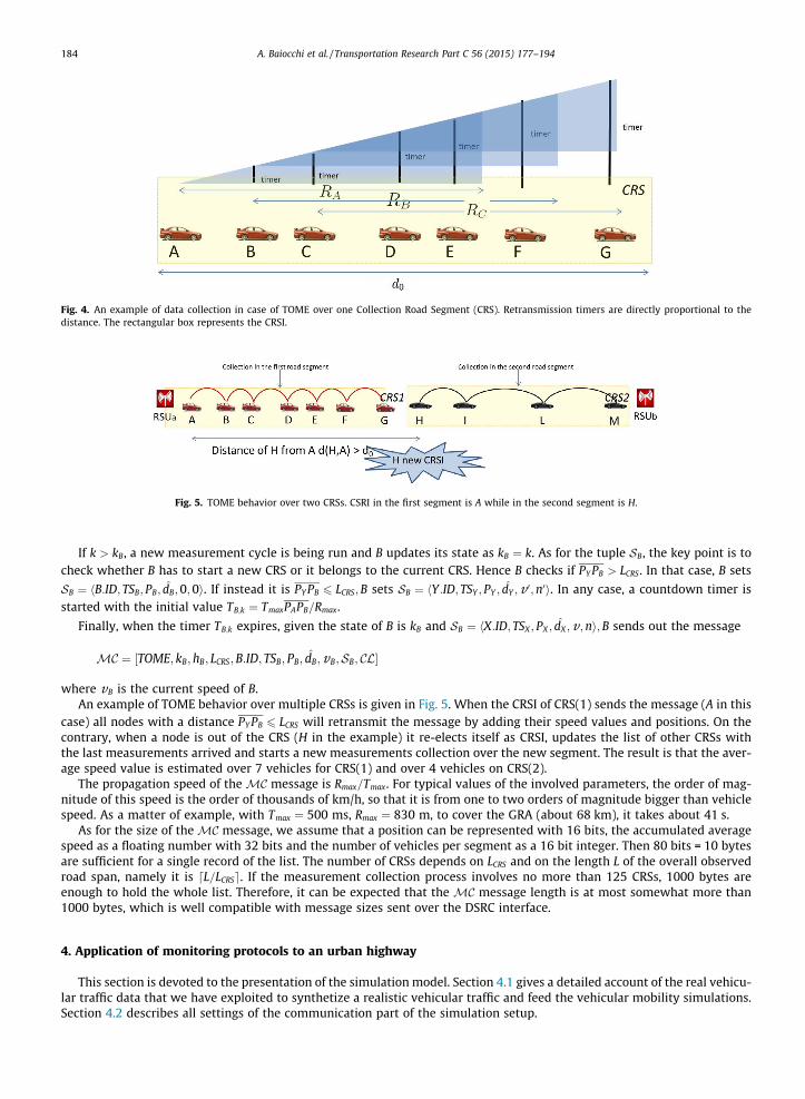
Fig. 4. An example of data collection in case of TOME over one Collection Road Segment (CRS). Retransmission timers are directly proportional to thedistance. The rectangular box represents the CRSI.

Fig. 5. TOME behavior over two CRSs. CSRI in the first segment is A while in the second segment is H.

184 A. Baiocchi et al. / Transportation Research Part C 56 (2015) 177–194

If k > kB, a new measurement cycle is being run and B updates its state as kB ¼ k. As for the tuple SB, the key point is tocheck whether B has to start a new CRS or it belongs to the current CRS. Hence B checks if PY PB > LCRS. In that case, B sets

SB ¼ hB:ID; TSB; PB; d̂B;0;0i. If instead it is PY PB 6 LCRS;B sets SB ¼ hY :ID; TSY ; PY ; d̂Y ; v 0;n0i. In any case, a countdown timer isstarted with the initial value TB;k ¼ TmaxPAPB=Rmax.

Finally, when the timer TB;k expires, given the state of B is kB and SB ¼ hX:ID; TSX ; PX ; d̂X ; v;ni; B sends out the message

MC ¼ ½TOME; kB; hB; LCRS;B:ID; TSB; PB; d̂B;vB;SB; CL�

where vB is the current speed of B.An example of TOME behavior over multiple CRSs is given in Fig. 5. When the CRSI of CRS(1) sends the message (A in this

case) all nodes with a distance PY PB 6 LCRS will retransmit the message by adding their speed values and positions. On thecontrary, when a node is out of the CRS (H in the example) it re-elects itself as CRSI, updates the list of other CRSs withthe last measurements arrived and starts a new measurements collection over the new segment. The result is that the aver-age speed value is estimated over 7 vehicles for CRS(1) and over 4 vehicles on CRS(2).

The propagation speed of the MC message is Rmax=Tmax. For typical values of the involved parameters, the order of mag-nitude of this speed is the order of thousands of km/h, so that it is from one to two orders of magnitude bigger than vehiclespeed. As a matter of example, with Tmax ¼ 500 ms, Rmax ¼ 830 m, to cover the GRA (about 68 km), it takes about 41 s.

As for the size of the MC message, we assume that a position can be represented with 16 bits, the accumulated averagespeed as a floating number with 32 bits and the number of vehicles per segment as a 16 bit integer. Then 80 bits = 10 bytesare sufficient for a single record of the list. The number of CRSs depends on LCRS and on the length L of the overall observedroad span, namely it is dL=LCRSe. If the measurement collection process involves no more than 125 CRSs, 1000 bytes areenough to hold the whole list. Therefore, it can be expected that the MC message length is at most somewhat more than1000 bytes, which is well compatible with message sizes sent over the DSRC interface.

4. Application of monitoring protocols to an urban highway

This section is devoted to the presentation of the simulation model. Section 4.1 gives a detailed account of the real vehicu-lar traffic data that we have exploited to synthetize a realistic vehicular traffic and feed the vehicular mobility simulations.Section 4.2 describes all settings of the communication part of the simulation setup.

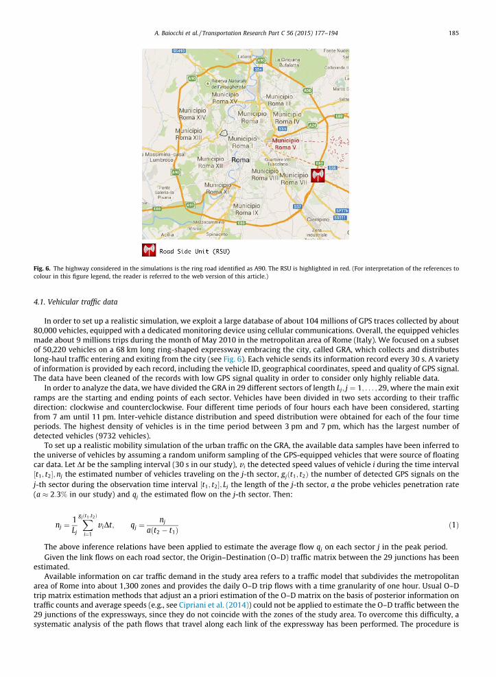
Fig. 6. The highway considered in the simulations is the ring road identified as A90. The RSU is highlighted in red. (For interpretation of the references tocolour in this figure legend, the reader is referred to the web version of this article.)

A. Baiocchi et al. / Transportation Research Part C 56 (2015) 177–194 185

4.1. Vehicular traffic data

In order to set up a realistic simulation, we exploit a large database of about 104 millions of GPS traces collected by about80,000 vehicles, equipped with a dedicated monitoring device using cellular communications. Overall, the equipped vehiclesmade about 9 millions trips during the month of May 2010 in the metropolitan area of Rome (Italy). We focused on a subsetof 50,220 vehicles on a 68 km long ring-shaped expressway embracing the city, called GRA, which collects and distributeslong-haul traffic entering and exiting from the city (see Fig. 6). Each vehicle sends its information record every 30 s. A varietyof information is provided by each record, including the vehicle ID, geographical coordinates, speed and quality of GPS signal.The data have been cleaned of the records with low GPS signal quality in order to consider only highly reliable data.

In order to analyze the data, we have divided the GRA in 29 different sectors of length Lj; j ¼ 1; . . . ;29, where the main exitramps are the starting and ending points of each sector. Vehicles have been divided in two sets according to their trafficdirection: clockwise and counterclockwise. Four different time periods of four hours each have been considered, startingfrom 7 am until 11 pm. Inter-vehicle distance distribution and speed distribution were obtained for each of the four timeperiods. The highest density of vehicles is in the time period between 3 pm and 7 pm, which has the largest number ofdetected vehicles (9732 vehicles).

To set up a realistic mobility simulation of the urban traffic on the GRA, the available data samples have been inferred tothe universe of vehicles by assuming a random uniform sampling of the GPS-equipped vehicles that were source of floatingcar data. Let Dt be the sampling interval (30 s in our study), v i the detected speed values of vehicle i during the time interval½t1; t2�;nj the estimated number of vehicles traveling on the j-th sector, gjðt1; t2Þ the number of detected GPS signals on thej-th sector during the observation time interval ½t1; t2�; Lj the length of the j-th sector, a the probe vehicles penetration rate(a � 2:3% in our study) and qj the estimated flow on the j-th sector. Then:

nj ¼1Lj

Xgjðt1 ;t2Þ

i¼1

v iDt; qj ¼nj

aðt2 � t1Þð1Þ

The above inference relations have been applied to estimate the average flow qj on each sector j in the peak period.Given the link flows on each road sector, the Origin–Destination (O–D) traffic matrix between the 29 junctions has been

estimated.Available information on car traffic demand in the study area refers to a traffic model that subdivides the metropolitan

area of Rome into about 1,300 zones and provides the daily O–D trip flows with a time granularity of one hour. Usual O–Dtrip matrix estimation methods that adjust an a priori estimation of the O–D matrix on the basis of posterior information ontraffic counts and average speeds (e.g., see Cipriani et al. (2014)) could not be applied to estimate the O–D traffic between the29 junctions of the expressways, since they do not coincide with the zones of the study area. To overcome this difficulty, asystematic analysis of the path flows that travel along each link of the expressway has been performed. The procedure is

186 A. Baiocchi et al. / Transportation Research Part C 56 (2015) 177–194

similar to the method implemented by Cipriani et al. (2006) to determine the optimal traffic count location on a road net-work. Given the traffic assignment in the time interval of interest, the fraction of the O–D trip flows that travels along eachentering ramp of the expressway and the corresponding traffic flows on all the links of the network, included the exit rampsof the expressway, have been computed. The envelope of the exit ramp flows for all entering ramps individuates the O–Dtraffic matrix from each entering ramp to every exit ramp for the whole expressway.

4.2. Simulation model

To simulate the traffic on the urban highway, we have imported the map of the Rome GRA from Open Street Map (e.g., seeHaklay and Weber, 2008) into SUMO (Behrisch et al., 2011). We have generated vehicular traffic flows on this map in accor-dance with what described in Section 4.1. We have implemented the VANET monitoring logics, as described in Section 3, byadding code to NS2 (Fall and Varadhan, 2000) to realize the SAME and TOME modules in the routing layer, on top of the IEEE802.11p MAC/PHY layers already built in NS2. The communication network simulations of NS2 have been fed by the out-come of SUMO to give node positions, sampled once per second. Between two consecutive sampling times, NS2 moves nodesaccording to linear uniform motion.

Since it will take years to deploy the VANET technology extensively, we have assumed different penetration percentagesof DSRC radio equipment on board vehicles. Because of this, we have assumed that every new vehicle that is instantiated inthe simulations is equipped with this technology with probability p 2 ½0;1�, which represents the penetration rate of theVANET technology. So, on average, only p � 100% of the vehicles are able to communicate with each other, while the othersdo not perform any transmission/reception operation, although influencing the vehicular micro-mobility simulated bySUMO.

We set up two simulation scenarios: (i) regular traffic conditions in the peak period identified through FCD collected onthe field (see Section 4); (ii) incident scenario, artificially generated in simulation. In the latter one, the flows are as in theregular scenario, except that we have placed still vehicles to obstruct two out of the three road lanes in one highway sectorand one direction per simulation.

The experiment is composed in the following way: for every highway sector we have 4 simulation runs, each lasting 100 sfor each value of p (we considered 3 of them) and for every sector (for a total of 29). We thus managed to have 348 sim-ulations of 100 s each, thus leading to 96.7 simulated hours. The main parameters of these simulations are listed in Table 2.

5. Performance evaluation

First results on stationary vehicular traffic monitoring are presented in Section 5.1. Then, the capability of SAME andTOME to provide evidence of vehicular traffic anomaly is explored in Section 5.2. An heuristic incident detection algorithmis defined and tested in Section 5.3.

5.1. Traffic monitoring in regular conditions

We assume regular traffic conditions on the considered urban highway and we feed vehicular traffic according to thestatistics derived from measurements in the peak time interval, as explained in Section 4. A single RSU is placed as shownin Fig. 6 and it acts contemporarily as MC message originator and sink. It sends out MC messages with a time periodTRSU ¼ 1 s.

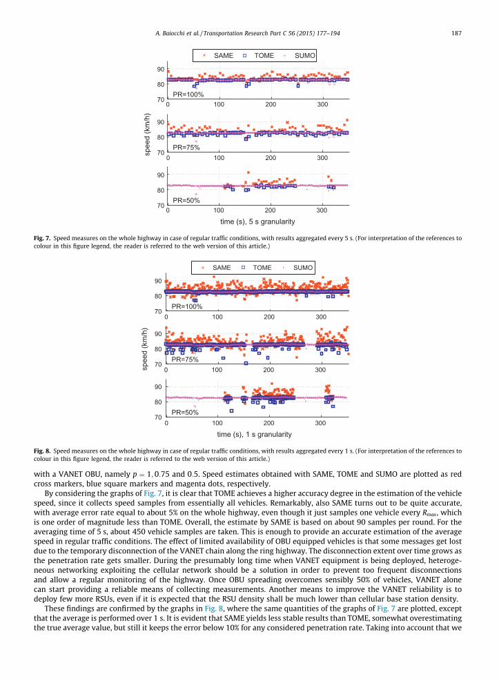
Figs. 7 and 8 plot the average speed measured over the entire urban highway through SAME and TOME and as given bythe simulation software SUMO (assumed as ground truth). Measurements collected by the RSU after a full trip of protocolmessages along the urban highway ring are averaged over a time window of 5 s in Fig. 7 and time window of 1 s inFig. 8. In each figure the three plots refer to different values of the Market Penetration Rate (MPR) p of vehicles equipped

Table 2Simulation parameter values.

Parameter Value

Road length, L (km) 68.2Number of lanes per traveling direction 3Average vehicle density (veh/km) 31:02SUMO simulation duration (s) 3600Network simulation duration (s) 400TRSU (s) 1Transmission power (mW) 500, 260, 100, 16, 8.7Rmax for each tx power value (m) 830, 700, 550, 350, 300Max forwarding delay, Tmax (ms) 100Link Rate (Mbit/s) 6MAC, PHY parameters IEEE 802.11pPropagation model Two ray ground

0 100 200 30070

80

90

PR=100%

0 100 200 30070

80

90

PR=75%sp

eed

(km

/h)

0 100 200 30070

80

90

PR=50%

time (s), 5 s granularity

SAME TOME SUMO

Fig. 7. Speed measures on the whole highway in case of regular traffic conditions, with results aggregated every 5 s. (For interpretation of the references tocolour in this figure legend, the reader is referred to the web version of this article.)

0 100 200 30070

80

90

PR=100%

0 100 200 30070

80

90

PR=75%

spee

d (k

m/h

)

0 100 200 30070

80

90

PR=50%

time (s), 1 s granularity

SAME TOME SUMO

Fig. 8. Speed measures on the whole highway in case of regular traffic conditions, with results aggregated every 1 s. (For interpretation of the references tocolour in this figure legend, the reader is referred to the web version of this article.)

A. Baiocchi et al. / Transportation Research Part C 56 (2015) 177–194 187

with a VANET OBU, namely p ¼ 1;0:75 and 0:5. Speed estimates obtained with SAME, TOME and SUMO are plotted as redcross markers, blue square markers and magenta dots, respectively.

By considering the graphs of Fig. 7, it is clear that TOME achieves a higher accuracy degree in the estimation of the vehiclespeed, since it collects speed samples from essentially all vehicles. Remarkably, also SAME turns out to be quite accurate,with average error rate equal to about 5% on the whole highway, even though it just samples one vehicle every Rmax, whichis one order of magnitude less than TOME. Overall, the estimate by SAME is based on about 90 samples per round. For theaveraging time of 5 s, about 450 vehicle samples are taken. This is enough to provide an accurate estimation of the averagespeed in regular traffic conditions. The effect of limited availability of OBU equipped vehicles is that some messages get lostdue to the temporary disconnection of the VANET chain along the ring highway. The disconnection extent over time grows asthe penetration rate gets smaller. During the presumably long time when VANET equipment is being deployed, heteroge-neous networking exploiting the cellular network should be a solution in order to prevent too frequent disconnectionsand allow a regular monitoring of the highway. Once OBU spreading overcomes sensibly 50% of vehicles, VANET alonecan start providing a reliable means of collecting measurements. Another means to improve the VANET reliability is todeploy few more RSUs, even if it is expected that the RSU density shall be much lower than cellular base station density.

These findings are confirmed by the graphs in Fig. 8, where the same quantities of the graphs of Fig. 7 are plotted, exceptthat the average is performed over 1 s. It is evident that SAME yields less stable results than TOME, somewhat overestimatingthe true average value, but still it keeps the error below 10% for any considered penetration rate. Taking into account that we

Fig. 9. Percentage error of vehicle speed estimated through SAME, with respect to the SUMO ground truth, displayed for various sampling ranges and for allhighway sectors.

188 A. Baiocchi et al. / Transportation Research Part C 56 (2015) 177–194

target real time vehicular traffic monitoring, we have to strike a balance between accuracy and delay. From our results, itappears that 5 s provides a sufficiently accurate estimation. This is much shorter than the usual aggregation intervals usedin fixed monitoring sensors, that are in the order of 30 s or longer.

The specific occurrences of the detected speed values for each sector are shown in the matrix of Fig. 9. For every sector ofthe highway, it gives the average error percentage of the values estimated by means of SAME with respect to the valuesobtained by SUMO simulations. Samples collected via SAME for each highway sector are aggregated over 1 s time windows.The number of averaged samples depends on the length of the road span of each sector: it is approximatively equal to theratio between the sector length and the average hop length.

The results displayed in Fig. 9 allow us to evaluate the speed estimation error as a function of the maximum hop rangeRmax, that determines the average sampling distance. The value of Rmax is tuned by adjusting the node transmission power.The obtained values in terms of Rmax match the experimental results obtained by Gozalvez et al. (2012) in similar scenarioand conditions.

The average error of speed estimates ranges from about 4.0% to about 5.5%, depending on the sampling distance. It can beconsidered a good result, if we compare this percentage with the random variability of the traffic. The analysis of FCD in thewhole metropolitan area, in fact, highlights that individual speeds have inter-vehicular coefficient of variation of 0.23 (andstandard deviation of 13 km/h), while the day-to-day variability of the average speed on the network has coefficient of varia-tion of 0.18 (and standard deviation of 11 km/h).

Errors are quite low in most sectors, namely wherever the traffic dynamics are easier to catch with just few samples(1 sample every Rmax). In other sectors, like #15, the monitoring process appears to be harder, so the error in particularlyunfavorable conditions can be even around 27%. This happens because the sector is too short with respect to Rmax and thusthe few samples collectedthere are not enough to get a low error with a granularity of 1 s. Errors can be reduced if we allowbigger smoothing time windows, e.g., by aggregating samples over times windows of 5 s, as shown in the graphs of Fig. 7.

A last consideration is about the required bit rate both for SAME and TOME: in the first case it is very low (0.08 kbps) andthis makes it possibile a permanent nearly invisible service, running on the control channel or on any non-dedicated sub-channel; in the second case, the bit rate is about 56 kbps, better suited for a channel explicitly dedicated to traffic monitoringservices.

5.2. Incident detection through VANET monitoring

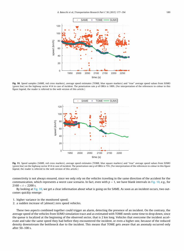
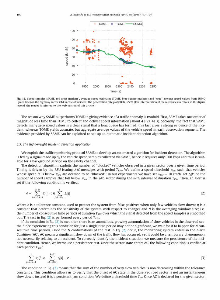
In this section we analyze the behavior of SAME and TOME under exceptional traffic conditions, caused by an incident.The results are depicted in Figs. 10–12. The results of these figures refer to a specific sector of the GRA, namely sector#14, the one where the incident had been introduced at time t ¼ 2000 s. In these plots we report the individual speed sam-ples collected with SAME within the tagged sector (red cross markers) and the average values estimated by TOME (bluesquare markers). The light green line shows the ‘‘true’’ average speed value, extracted by the SUMO traces.

It is clear that in this case the penetration rate is a very important factor, since after the incident occurs, the vehicle flow isstrongly slowed down and becomes irregular in the interested sector. In terms of communications, this means that

1950 2000 2050 2100 2150 2200 22500

20

40

60

80

100

120

time (s)

spee

d (k

m/h

)

SAME TOME SUMO

Fig. 10. Speed samples (SAME, red cross markers), average speed estimates (TOME, blue square markers) and ‘‘true’’ average speed values from SUMO(green line) on the highway sector #14 in case of incident. The penetration rate p of OBUs is 100%. (For interpretation of the references to colour in thisfigure legend, the reader is referred to the web version of this article.)

1950 2000 2050 2100 2150 22000

20

40

60

80

100

120

time (s)

spee

d (k

m/h

)

SAME TOME SUMO

Fig. 11. Speed samples (SAME, red cross markers), average speed estimates (TOME, blue square markers) and ‘‘true’’ average speed values from SUMO(green line) on the highway sector #14 in case of incident. The penetration rate p of OBUs is 75%. (For interpretation of the references to colour in this figurelegend, the reader is referred to the web version of this article.)

A. Baiocchi et al. / Transportation Research Part C 56 (2015) 177–194 189

connectivity is not always ensured, since we only rely on the vehicles traveling in the same direction of the accident for thecommunication, which represents a worst case scenario. In fact, even with p ¼ 1, we have blank intervals in Fig. 10, e.g., for2160 < t < 2200 s.

By looking at Fig. 10, we get a clear information about what is going on for SAME. As soon as an incident occurs, two out-comes quickly emerge:

1. higher variance in the monitored speed;2. a sudden increase of (almost) zero speed vehicles.

These two aspects combined together could trigger an alarm, detecting the presence of an incident. On the contrary, theaverage speed of the vehicles from SUMO simulation trace and as estimated with TOME needs some time to drop down, sincethe queue is localized at the beginning of the observed sector, that is 2 km long. Vehicles that overcome the incident accel-erate and take the same speed they had before they encountered the incident, or even a higher one, because of the reduceddensity downstream the bottleneck due to the incident. This means that TOME gets aware that an anomaly occurred onlyafter 50–100 s.

1950 2000 2050 2100 2150 2200 22500

20

40

60

80

100

120

time (s)

spee

d (k

m/h

)

SAME TOME SUMO

Fig. 12. Speed samples (SAME, red cross markers), average speed estimates (TOME, blue square markers) and ‘‘true’’ average speed values from SUMO(green line) on the highway sector #14 in case of incident. The penetration rate p of OBUs is 50%. (For interpretation of the references to colour in this figurelegend, the reader is referred to the web version of this article.)

190 A. Baiocchi et al. / Transportation Research Part C 56 (2015) 177–194

The reason why SAME outperforms TOME in giving evidence of a traffic anomaly is twofold. First, SAME takes one order ofmagnitude less time than TOME to collect and deliver speed information (about 4 s vs. 41 s). Secondly, the fact that SAMEdetects many zero speed values is a clear signal that a long queue has formed: this fact gives a strong evidence of the inci-dent, whereas TOME yields accurate, but aggregate average values of the vehicle speed in each observation segment. Theevidence provided by SAME can be exploited to set up an automatic incident detection algorithm.

5.3. The light-weight incident detection application

We exploit the traffic monitoring protocol SAME to develop an automated algorithm for incident detection. The algorithmis fed by a signal made up by the vehicle speed samples collected via SAME, hence it requires only 0.08 kbps and thus is suit-able for a background service on the safety channel.

The detection algorithm exploits the number of ‘‘blocked’’ vehicles observed in a given sector over a given time period.Timing is driven by the RSU issuing MC messages with period TRSU . We define a speed threshold v low such that vehicleswhose speed falls below v low are deemed to be ‘‘blocked’’; in our experiments we have set v low ¼ 10 km/h. Let zs½k� be thenumber of speed samples that fall below v low in the j-th sector during the k-th interval of duration TRSU . Then, an alert isset if the following condition is verified:

eþXk�N

i¼k�2Nþ1

zs½i� < gXk

j¼k�Nþ1

zs½j� ð2Þ

where e is a tolerance constant, used to protect the system from false positives when only few vehicles slow down; g is aconstant that determines the sensitivity of the system with respect to changes and N is the averaging window size; i.e.,the number of consecutive time periods of duration TRSU over which the signal detected from the speed samples is smoothedout. The test in Eq. (2) is performed every period TRSU .

If the condition in Eq. (2) is met, then there is an anomalous, growing accumulation of slow vehicles in the observed sec-tor. Since experiencing this condition for just a single time period may not be significant, we wait for it to happen for N con-secutive time periods. Once the N confirmations of the test in Eq. (2) occur, the monitoring system enters in the AlarmCondition (AC). AC means a significant slow down of the traffic flow has occurred, yet it could be a temporary phenomenon,not necessarily relating to an accident. To correctly identify the incident situation, we measure the persistence of the inci-dent condition. Hence, we introduce a persistence test. Once the sector state enters AC, the following condition is verified ateach period TRSU:

Xk

j¼k�Nþ1

zs½j�PXk�N

i¼k�2Nþ1

zs½i� � e ð3Þ

The condition in Eq. (3) means that the sum of the number of very slow vehicles is non decreasing within the toleranceconstant e. This condition allows us to verify that the onset of AC state in the observed road sector is not an instantaneousslow down, instead it is a persistent jam condition. We define a threshold time Tpe. Once AC is declared for the given sector,

0 50 100 150 200 250 3000

50

100

150

200

250

time after incident (s)

Que

ue le

ngth

(m)

Lane 0Lane 1Notification time, penetration 1Notification time, penetration 0.75Notification time, penetration 0.5

Fig. 13. Average queue length for the two lanes blocked by the incident. The vertical lines display the algorithm notification time as a function of the DSRCpenetration rate.

A. Baiocchi et al. / Transportation Research Part C 56 (2015) 177–194 191

the algorithm detects an incident only if the persistence time is at least equal to Tpe. Therefore, an AC state is turned into anincident alarm only if the test in Eq. (3) holds for K ¼ dTpe=TRSUe consecutive TRSU intervals. Once the condition in Eq. (3)becomes false, the incident alarm is switched off.

To create a wide variety of different conditions, we have simulated in turn an incident in each one of the 29 sectors of theconsidered highway (a single incident in each simulations). The incident corresponds to blocking two out of three lanes ofthe highway at a given time instant. We measure the incident detection delay D defined as the time that goes from theinstant in which the incident actually takes place to the instant in which the RSU declares the incident occurrence, accordingto the criterion in Eqs. (2) and (3). The incident detection delay includes all the transmission delays and the processing timeto understand that an incident took place.

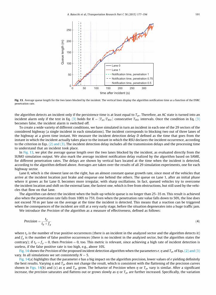
In Fig. 13, we plot the average queue length over the two lanes blocked by the incident, as evaluated directly from theSUMO simulation output. We also mark the average incident notification delay realized by the algorithm based on SAME,for different penetration rates. The delays are shown by vertical bars located at the time when the incident is detected,according to the algorithm defined above. Averages are taken over the results of all 29 simulation experiments, one for eachhighway sector.

Lane 0, which is the slowest lane on the right, has an almost constant queue growth rate, since most of the vehicles thatarrive at the incident location just brake and enqueue one behind the others. The queue on Lane 1, after an initial phasewhere it grows as for Lane 0, becomes more irregular, with sharp oscillations. In fact, queued vehicles try to overcomethe incident location and shift on the external lane, the fastest one, which is free from obstructions, but still used by the vehi-cles that flow on that lane.

The algorithm can detect the incident when the built-up vehicle queue is no longer than 25–35 m. This result is achievedalso when the penetration rate falls from 100% to 75%. Even when the penetration rate value falls down to 50%, the line doesnot exceed 70 m per lane on the average at the time the incident is detected. This means that a reaction can be triggeredwhen the consequences of the incident are still at a very early stage, before the situation degenerates into a huge traffic jam.

We introduce the Precision of the algorithm as a measure of effectiveness, defined as follows:

Precision ¼ tp

tp þ f pð4Þ

where tp is the number of true positive occurrences (there is an incident in the analyzed sector and the algorithm detects it)and f p is the number of false positive occurrences (there is no incident in the analyzed sector, but the algorithm states thecontrary); if tp ¼ f p ¼ 0, then Precision ¼ 0, too. This metric is relevant, since achieving a high rate of incident detection isuseless, if the false positive rate is too high, e.g., above 10%.

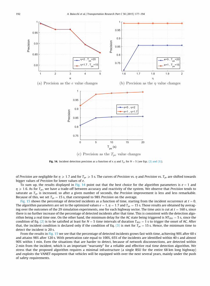
Fig. 14 shows the Precision of the proposed incident detection algorithm when the parameters e;g and Tpe of Eqs. (2) and (3)vary. In all simulations we set consistently N ¼ 5.

Fig. 14(a) highlights that the parameter e has a big impact on the algorithm precision, lower values of e yielding definitelythe best results. Varying g and Tpe does not change the result, which is consistent with the flattening of the precision curvesshown in Figs. 14(b) and (c) as g and Tpe grow. The behavior of Precision when g or Tpe vary is similar. After a significantincrease, the precision saturates and flattens out or grows slowly as g or Tpe are further increased. Specifically, the variation

1 2 3 4 5

0.8

0.85

0.9

0.95

1

e

Prec

isio

n

η=2 , Tpe=20

η=1.7 , Tpe=15

(a) Precision as the e value changes

1.6 1.7 1.8 1.9 2

0.75

0.8

0.85

0.9

0.95

1

η

Prec

isio

n

e=5 , Tpe=20

e=1 , Tpe=15

(b) Precision as the η value changes

0 5 10 15 20

0.75

0.8

0.85

0.9

0.95

1

Tpe (s)

Prec

isio

n

e=5 , η=2e=1 , η=1.7

(c) Precision as the Tpe value changes

Fig. 14. Incident detection precision as a function of e;g and Tpe for N ¼ 5 (see Eqs. (2) and (3)).

192 A. Baiocchi et al. / Transportation Research Part C 56 (2015) 177–194

of Precision are negligible for g P 1:7 and for Tpe P 5 s. The curves of Precision vs. g and Precision vs. Tpe are shifted towardsbigger values of Precision for lower values of e.

To sum up, the results displayed in Fig. 14 point out that the best choice for the algorithm parameters is e ¼ 1 andg P 1:6. As for Tpe, we have a trade-off between accuracy and reactivity of the system. We observe that Precision tends tosaturate as Tpe is increased, so after a given number of seconds, the Precision improvement is less and less remarkable.Because of this, we set Tpe ¼ 15 s, that correspond to 98% Precision on the average.

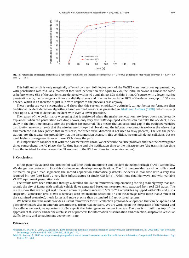
Fig. 15 shows the percentage of detected incidents as a function of time, starting from the incident occurrence at t ¼ 0.The algorithm parameters are set to the optimized values e ¼ 1;g ¼ 1:7 and Tpe ¼ 15 s. Those results are obtained by averag-ing over the outcomes of the 29 simulation experiments, one for each highway sector. The time axis is cut at t ¼ 160 s, sincethere is no further increase of the percentage of detected incidents after that time. This is consistent with the detection algo-rithm being a real time one. On the other hand, the minimum delay for the AC state being triggered is NTRSU ¼ 5 s, since thecondition of Eq. (2) is to be satisfied at least for N ¼ 5 time intervals of duration TRSU ¼ 1 s to trigger the onset of AC. Afterthat, the incident condition is declared only if the condition of Eq. (3) is met for Tpe ¼ 15 s. Hence, the minimum time todetect the incident is 20 s.

From the results in Fig. 15 we see that the percentage of detected incidents grows fast with time, achieving 90% after 60 sand attains 98% after 120 s. With penetration rate equal to 100%, 65% of the incidents are identified within 40 s and almost90% within 1 min. Even the situations that are harder to detect, because of network disconnections, are detected within2 min from the incident, which is an important ‘‘warranty’’ for a reliable and effective real time detection algorithm. Westress that the proposed algorithm requires a minimal infrastructure (a single RSU for the entire 68 km long highway)and exploits the VANET equipment that vehicles will be equipped with over the next several years, mainly under the pushof safety requirements.

0 20 40 60 80 100 120 140 1600

102030405060708090

100

time (s)

Perc

enta

ge o

f det

ecte

d in

cide

nts

(%)

Penetration=75%Penetration=100%

Fig. 15. Percentage of detected incidents as a function of time after the incident occurrence at t ¼ 0 for two penetration rate values and with e ¼ 1;g ¼ 1:7and Tpe ¼ 15 s.

A. Baiocchi et al. / Transportation Research Part C 56 (2015) 177–194 193

This brilliant result is only marginally affected by a non full deployment of the VANET communication equipment, i.e.,with penetration rate 75%. As a matter of fact, with penetration rate equal to 75%, the initial behavior is almost the sameas before, where 65% of the accidents are detected within 40 s and almost 80% within 1 min. Of course, with a lower marketpenetration rate, the convergence times are slightly slower and in order to reach the 100% of the detections, up to 160 s areneeded, which is an increase of just 40 s with respect to the previous case anyway.

These results are very encouraging and show that this system, empirically optimized, can get better performance thantraditional incident detection algorithms based on fixed sensors, as presented in Ishak and Al-Deek (1998), which usuallyneed up to 6–8 min to detect an incident with even a lower precision.

The reason of the performance worsening that is registered when the market penetration rate drops down can be easilyexplained: when the penetration rate drops down, only very few DSRC-equipped vehicles can overtake the accident, espe-cially in the first time instants after the problem has occurred. This means that an occasional gap in the equipped vehiclesdistribution may occur, such that the wireless multi-hop chain breaks and the information cannot travel over the whole ringand reach the RSU back (notice that in this case, the other travel direction is not used to relay packets). The less the pene-tration rate, the greater the probability that the disconnection occurs. In this condition, we can still detect collisions, but weneed higher convergence times or more RSUs along the path.

It is important to consider that with the parameters we chose, we experience no false positives and that the convergencetimes comprehend the AC phase, the Tpe time frame and the notification time to the infrastructure (the transmission timefrom the incident location across the 68 km road to the RSU and thus to the service center).

6. Conclusions

In this paper we address the problem of real time traffic monitoring and incident detection through VANET technology.We design two protocols to face this challenge and develop two applications. The first one provides real-time traffic speedestimates on given road segments; the second application automatically detects incidents in real time with a very lowrequired bit rate (0.08 kbps), a very light infrastructure (a single RSU for a �70 km long ring highway), and with variableVANET equipment penetration rate.

The results have been validated through a detailed simulation framework, implementing the ring road highway that sur-rounds the city of Rome, with realistic vehicle flows generated based on measurements extracted from real GPS traces. Theresults show that we can get real time and accurate performance with 50% to 75% of vehicles equipped with OBUs and just asingle RSU: a precision level of 98% is achieved with fast incident detection (47 s on the average, never more than 2 min in allthe examined scenarios), much faster and more precise than a standard infrastructured system.

We believe that this work provides a useful framework for FCD collection protocol development, that can be applied andpossibly extended also in different scenarios, e.g., urban road network. We are working on the integration of the VANET andthe cellular network, to opportunistically exploit the heterogeneous network access. The aim is to build on top of theapproach of this work and define a robust set of protocols for information dissemination and collection, adaptive to vehiculartraffic density and to equipment deployment rate.

References

Abuelela, M., Olariu, S., Cetin, M., Rawat, D., 2009. Enhancing automatic incident detection using vehicular communications. In: 2009 IEEE 70th VehicularTechnology Conference Fall (VTC 2009-Fall). IEEE, pp. 1–5.

Adeli, H., Samant, A., 2000. An adaptive conjugate gradient neural network–wavelet model for traffic incident detection. Comput.-Aid. Civil Infrastruct. Eng.15 (4), 251–260.

194 A. Baiocchi et al. / Transportation Research Part C 56 (2015) 177–194

Ahmed, S.A., Cook, A.R., 1982. Application of time-series analysis techniques to freeway incident detection. Transport. Res. Rec. 1 (841), 19–21.Barcelò, J., Montero, L., Bullejos, M., Serch, O., Carmona, C., 2013. A Kalman filter approach for exploiting bluetooth traffic data when estimating time-

dependent OD matrices. J. Intell. Transport. Syst.: Technol. Plann. Oper. 17 (2), 123–141.Bauza, R., Gozálvez, J., 2013. Traffic congestion detection in large-scale scenarios using vehicle-to-vehicle communications. J. Netw. Comput. Appl. 36 (5),

1295–1307.Behrisch, M., Bieker, L., Erdmann, J., Krajzewicz, D., 2011. Sumo-simulation of urban mobility-an overview. In: SIMUL 2011, The Third International

Conference on Advances in System Simulation, pp. 55–60.Borsetti, D., Fiore, M., Casetti, C., Chiasserini, C.-F., 2011. An application-level framework for information dissemination and collection in vehicular networks.

Perform. Eval. 68 (9), 876–896, special Issue: Advances in Wireless and Mobile Networks.Cipriani, E., Fusco, G., Gori, S., Petrelli, M., 2006. Heuristic methods for the optimal location of road traffic monitoring. In: Intelligent Transportation Systems

Conference, 2006. ITSC ’06. IEEE, pp. 1072–1077.Cipriani, E., Nigro, M., Fusco, G., Colombaroni, C., 2014. Effectiveness of link and path information on simultaneous adjustment of dynamic o–d demand

matrix. Eur. Transport Res. Rev. 6 (2), 139–148.De Felice, M., Baiocchi, A., Cuomo, F., Fusco, G., Colombaroni, C., April 2014. Traffic monitoring and incident detection through vanets. In: 2014 11th Annual

Conference on Wireless On-demand Network Systems and Services (WONS), pp. 122–129.Dia, H., Thomas, K., 2011. Development and evaluation of arterial incident detection models using fusion of simulated probe vehicle and loop detector data.

Inform. Fusion 12 (1), 20–27.Dudek, C.L., Messer, C.J., Nuckles, N.B., 1974. Incident detection on urban freeways. In: Proceedings of the 53rd Annual Meeting of the Highway Research

Board, pp. 12–24.Fall, K., Varadhan, K., 2000. ns notes and documents. The VINT Project, UC Berkeley, LBL, USC/ISI, and Xerox PARC.Geisler, S., Quix, C., Schiffer, S., Jarke, M., 2012. An evaluation framework for traffic information systems based on data streams. Transport. Res. Part C:

Emerg. Technol. 23, 29–55.Gozalvez, J., Sepulcre, M., Bauza, R., 2012. Ieee 802.11p vehicle to infrastructure communications in urban environments. Commun. Mag. IEEE 50 (5), 176–

183.Haklay, M., Weber, P., 2008. Openstreetmap: user-generated street maps. Pervasive Comput. IEEE 7 (4), 12–18.Hsiao, C.-H., Lin, C.-T., Cassidy, M., 1994. Application of fuzzy logic and neural networks to automatically detect freeway traffic incidents. J. Transport. Eng.

120 (5), 753–772.Ishak, S.S., Al-Deek, H.M., 1998. Fuzzy art neural network model for automated detection of freeway incidents. Transport. Res. Rec.: J. Transport. Res. Board

1634 (1), 56–63.Khorashadi, B., Liu, F., Ghosal, D., Zhang, M., Chuah, C.-N., 2011. Distributed automated incident detection with vgrid. Wireless Commun. IEEE 18 (1), 64–73.Li, L., Wen, D., Yao, D., 2014. A survey of traffic control with vehicular communications. IEEE Trans. Intell. Transport. Syst. 15 (1), 425–432.Lin, C.-K., Chang, G.-L., 1998. Development of a fuzzy-expert system for incident detection and classification. Math. Comput. Modell. 27 (9), 9–25.Long Cheu, R., Xie, C., Lee, D.-H., 2002. Probe vehicle population and sample size for arterial speed estimation. Comput.-Aid. Civil Infrastruct. Eng. 17 (1), 53–

60.Ma, Y., Chowdhury, M., Sadek, A., Jeihani, M., 2009. Real-time highway traffic condition assessment framework using vehicle–infrastructure integration (vii)

with artificial intelligence (ai). IEEE Trans. Intell. Transport. Syst. 10 (4), 615–627.Mahmassani, H.S., Haas, C., Zhou, S., Peterman, J., 1998. Evaluation of incident detection methodologies. Research Report.Ni, S.-Y., Tseng, Y.-C., Chen, Y.-S., Sheu, J.-P., 1999. The broadcast storm problem in a mobile ad hoc network. In: Proceedings of the 5th Annual ACM/IEEE

International Conference on Mobile Computing and Networking, MobiCom ’99, pp. 151–162.Payne, H., Tignor, S., 1978. Freeway incident-detection algorithms based on decision trees with states. Transport. Res. Rec. 1 (682), 30–37.Persaud, B.N., Hall, F.L., Hall, L.M., 1990. Congestion identification aspects of the mcmaster incident detection algorithm. Transport. Res. Rec. 1 (1287), 167–

175.Santamaria, A.F., Sottile, C., Lupia, A., Raimondo, P., 2014. An efficient traffic management protocol based on ieee802. 11p standard. In: International

Symposium on Performance Evaluation of Computer and Telecommunication Systems (SPECTS 2014). IEEE, pp. 634–641.Sermons, M.W., Koppelman, F.S., 1996. Use of vehicle positioning data for arterial incident detection. Transport. Res. Part C: Emerg. Technol. 4 (2), 87–96.Sommer, C., Eckhoff, D., German, R., Dressler, F., 2011. A computationally inexpensive empirical model of ieee 802.11p radio shadowing in urban

environments. In: 2011 Eighth International Conference on Wireless On-Demand Network Systems and Services (WONS). IEEE, pp. 84–90.Stephanedes, Y.J., Chassiakos, A.P., 1993. Freeway incident detection through filtering. Transport. Res. Part C: Emerg. Technol. 1 (3), 219–233.Stephanedes, Y.J., Liu, X., 1995. Artificial neural networks for freeway incident detection. Transport. Res. Rec. 1 (1494), 91–97.Terroso-Sáenz, F., Valdés-Vela, M., Sotomayor-Martínez, C., Toledo-Moreo, R., Gómez-Skarmeta, A.F., 2012. A cooperative approach to traffic congestion

detection with complex event processing and vanet. IEEE Trans. Intell. Transport. Syst. 13 (2), 914–929.Vlahogianni, E.I., Karlaftis, M.G., Golias, J.C., 2014. Short-term traffic forecasting: where we are and where were going. Transport. Res. Part C: Emerg. Technol.

43 (Part 1), 3–19.Wang, J., Li, X., Liao, S., Hua, Z., 2013. A hybrid approach for automatic incident detection. IEEE Trans. Intell. Transport. Syst. 14 (3), 1176–1185.Yin, K., Wang, X.B., Zhang, Y., 2013. Vehicle-to-vehicle connectivity on two parallel roadways with a general headway distribution. Transport. Res. Part C:

Emerg. Technol. 29, 84–96.