JOURNAL OF OPERATIONS MANAGEMENT--SPECIAL COMBINED ISSUE

Vol. 6, No. 4, August 1986

Exponentially Smoothed Regression Analysis for Demand Forecasting

GARY M. ROODMAN*

EXECUTIVE SUMMARY

This article proposes a new technique for estimating trend and multiplicative scasonality in time

series data. The technique is computationally quite straightforward and gives better forecasts (in a

sense described below) than other commonly used methods. Like many other methods, the one

presented here is basically a decomposition technique, that is, it attempts to isolate and estimate

the several subcomponents in the time series. It draws primarily on regression analysis for its

power and has some of the computational advantages of exponential smoothing. In particular, old

estimates of base, trend, and seasonality may be smoothed with new data as they occur. The basic

technique was developed originally as a way to generate initial parameter values for a Winters

exponential smoothing model [4], but it proved to be a useful forecasting method in itself.

The objective in all decomposition methods is to separate somehow the effects of trend and

seasonahty in the data, so that the two may be estimated independently. When seasonality is

modeled with an additive form (Datum = Base + Trend + Seasonal Factor), techniques such as

regression analysis with dummy variables or ratio-to-moving-average techniques accomplish this

task well. It is more common, however, to model seasonality as a multiplicative form (as in the

Winters model, for example, where Datum = [Base + Trend] * Seasonal Factor). In this case, it

can be shown that neither of the techniques above achieves a proper separation of the trend and

seasonal effects, and in some instances may give highly misleading results. The technique described

in this article attempts to deal properly with multiplicative seasonality, while remaining computa-

tionally tractable.

The technique is built on a set of simple regression models, one for each period in the seasonal

cycle. These models are used to estimate individual seasonal effects and then pooled to estimate

the base and trend. As new data occur, they are smoothed into the least-squares formulas with

computations that are quite similar to those used in ordinary exponential smoothing. Thus, the

full least-squares computations are done only once, when the forecasting process is first initiated.

Although the technique is demonstrated here under the assumption that trend is linear, the trend

may, in fact, assume any form for which the curve-fitting tools are available (exponential, polynomial, etc.).

The method has proved to be easy to program and execute, and computational experience has

been quite favorable. It is faster than the RTMA method or regression with dummy variables

(which requires a multiple regression routine), and it is competitive with, although a bit slower than, ordinary triple exponential smoothing.

* State University of New York, Binghamton, New York.

Journal of Operations Management 485

INTRODUmION

This article proposes a new technique for estimating trend and multiplicative seasonality in time series data. The technique is computationally quite straightfonvard and gives better estimates (in a sense described below) than other commonly used methods. The technique is basically a decomposition method, that is, it attempts to isolate and estimate the several subcomponents in a time series. It draws primarily on regression analysis for its power, however, and has some of the computational advantages of exponential smoothing methods. In particular, old estimates may be smoothed with new data as they occur. The basic tech- nique was developed originally as a way to generate initial parameter values for a Winters exponential smoothing model [4], but it has proved to be a useful forecasting method in itself.

The first section below briefly examines a few commonly used forecasting techniques to establish the contribution that the new procedure can make. Then, the new procedure is stated in its simplest form in the second section, followed by the full exponentially smoothed regression model in the third section. The article concludes with a brief discussion of several possible extensions. The appendix to the article contains a set of examples. Several of these simply demonstrate the application of the technique to small data sets, and one applies the method to a larger body of real data.

SOME STANDARD TECHNIQUES

The object in all decomposition methods is to separate somehow the effects of trend and seasonality in the data, so that the two components can be estimated independently. To do this, a transformation is performed on the data to deseasonalize it (thereby isolating the trend) or detrend it (to get at the seasonality).

In ratio-to-moving averages techniques, for example, it is necessary to compute for each period a moving average that is intended to average away the seasonality in the data, along with some of the randomness. These moving averages then provide the base from which seasonal variations are measured and the trend is estimated (see Makridakis, Wheelwright, and McGee [2]). Regression analysis with dummy variables is another approach to achieving similar ends. In this case, the dummy variables serve to model the differences among seasons (as reflected in the intercept coefficient) and the slope coefficient is a measure of the trend.

These two techniques, and others that have been proposed for the same purpose, work well as long as the seasonality in the data can properly be modelled as an additive form (i.e., Datum = Base + Trend + Seasonal Factor). When seasonality is multiplicative, however (Datum = [Base + Trend] *Seasonal Factor), it can be shown that neither one achieves a complete separation of the trend and seasonal effects (see Roodman [3]). In the case of the RTMA technique, the moving averages do not truly average away the seasonality when it has a multiplicative form; indeed they would not, even if there were no randomness in the data. In regression analysis with dummy variables, the problem arises because both base (intercept) and trend (slope) vary with the seasons for multiplicative seasonality, a fact that the dummy variable mechanism cannot capture.

The technique that is now described attempts to deal properly with the case of multipli- cative seasonality, while retaining most of the computational tractability that typically char- acterizes decomposition methods.

466 APICS

BASIC ESTIMATION PROCEDURE

The procedure will be stated here assuming that trend has a linear form, although it would also be valid if trend were nonlinear. For simplicity of exposition, the periods in the seasonal cycle will be referred to as “quarters,” although it will be clear that they could as

well be “months,” “weeks,” etc. Let n be the number of data points in the initial time series and Q the number of periods

(quarters) in one seasonal cycle. Then define the sets

x,= {tit= 1,. . . ,nandtmodQ=q} q= 1,. . . ,Q

As defined, X, is the set of all t-indices for quarter q. The process that generates the data for all periods t that fall in quarter q is given by

Yt=(/3+7*t)*cq+e tEX, (1)

where

Y, = the datum for period t ,6 = base demand at the beginning of the time series horizon T = the linear trend per quarter

uq = the multiplicative seasonal factor for quarter q, e = a disturbance term

This will be the model used throughout the article. A four-step procedure is proposed for estimating /3,~, and (TV, q = 1, . . . , Q. The procedure

is stated below in its simplest form, together with the motivation for each step. MODEL EACH QUARTER. Using simple regression analysis, model each quarter in the seasonal cycle separately. Let

Y,=a,+b,*t tEX, (2)

denote the least-squares line for quarter q, q = 1, * - - Q. The seasonal variation in the data may be inputed from this set of Q models. If (1) is rewritten as

Y,=[/3*aq]+[7*flq]*t+e

it is clear that a, is an estimator of [p * cq] and b, is an estimator of [T * uq]. Consequently, the ratio of cq to gI may be estimated from the ratio %,/a,. It may also be estimated from b,/b,, or from any ratio of the form [as + b,*t]/[a, + b1 * t] for specified t. ESTIMATE SEASONALITY. Let S, denote the estimate of uq, q = 1, . . . , Q. Select one quarter, say, Quarter 1, as the “base” quarter and set S, = 1. Then compute S,, q = 2, . . . , Q as

” S, = [a, + b,*A]/[ar + br *A]

where A = C t/n. The choice of A here, among all possible values oft, is based on t= I

the fact that the variance of the estimators in both the numerator and denominator of the ratio are smallest in the neighborhood of the mean oft (Johnston [ 11). DESEASONALIZE THE DATA. Deseasonalize the data by dividing each Y, by the appropriate seasonal factor, generating a new time series, Zr , . . . , Z,. ESTIMATE TREND AND BASE. Let B and T denote estimates of /3 and T, respec- tively. Compute B and T by fitting a least-squares regression line to the deseasonalized data,

Zt=B+T*t

Journal of Operations Management 487

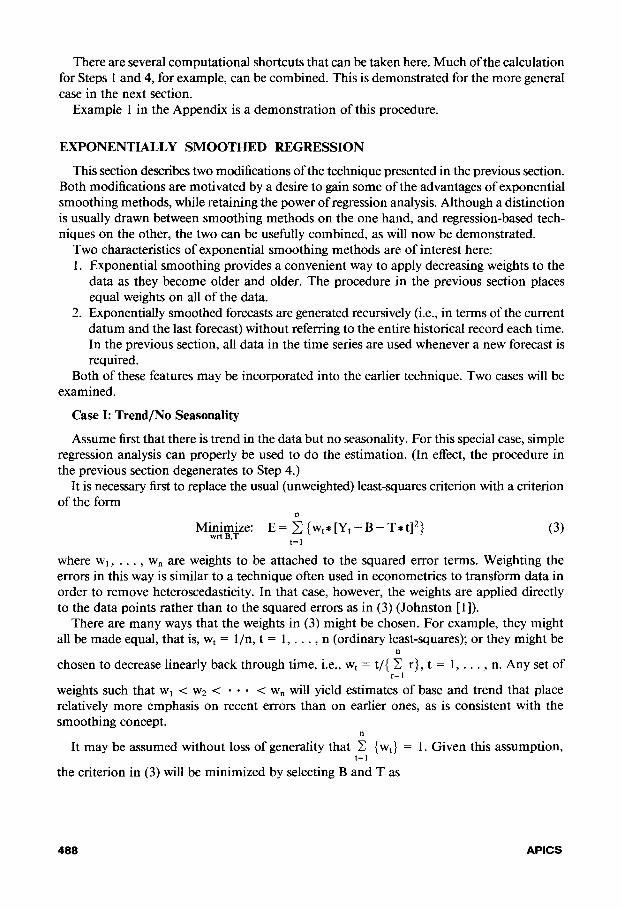
There are several computational shortcuts that can be taken here. Much of the calculation for Steps 1 and 4, for example, can be combined. This is demonstrated for the more general case in the next section.

Example 1 in the Appendix is a demonstration of this procedure.

EXPONENTIALLY SMOOTHED REGRESSION

This section describes two modifications of the technique presented in the previous section. Both modifications are motivated by a desire to gain some of the advantages of exponential smoothing methods, while retaining the power of regression analysis. Although a distinction is usually drawn between smoothing methods on the one hand, and regression-based tech- niques on the other, the two can be usefully combined, as will now be demonstrated.

Two characteristics of exponential smoothing methods are of interest here: 1. Exponential smoothing provides a convenient way to apply decreasing weights to the

data as they become older and older. The procedure in the previous section places equal weights on all of the data.

2. Exponentially smoothed forecasts are generated recursively (i.e., in terms of the current datum and the last forecast) without referring to the entire historical record each time. In the previous section, all data in the time series are used whenever a new forecast is required.

Both of these features may be incorporated into the earlier technique. Two cases will be examined.

Case I: Trend/No Seasonality

Assume first that there is trend in the data but no seasonality. For this special case, simple regression analysis can properly be used to do the estimation. (In effect, the procedure in the previous section degenerates to Step 4.)

It is necessary first to replace the usual (unweighted) least-squares criterion with a criterion of the form

n Mi@&ze: E= c {w&Y,-B-T*t]‘}

t=1

where wl, . . . , w, are weights to be attached to the squared error terms. Weighting the errors in this way is similar to a technique often used in econometrics to transform data in order to remove heteroscedasticity. In that case, however, the weights are applied directly to the data points rather than to the squared errors as in (3) (Johnston [ 11).

There are many ways that the weights in (3) might be chosen. For example, they might all be made equal, that is, w, = l/n, t = 1, . . . , n (ordinary least-squares); or they might be

chosen to decrease linearly back through time, i.e., w, = t/{ 5 r), t = 1, . . . , n. Any set of r=l

weights such that w1 < w2 < - - - < w, will yield estimates of base and trend that place relatively more emphasis on recent errors than on earlier ones, as is consistent with the smoothing concept.

It may be assumed without loss of generality that g {wt} = 1. Given this assumption, t=l

the criterion in (3) will be minimized by selecting B and T as

488 APICS

T=[WSl-WS3*WS4]

[ ws2 - ws47

B=[WS3-T*WS4]

(4)

(5)

where

WSl = i {w,*t*YJ t=1

ws2 = f: {w,*t*t} t=1

ws3 = E {w,*Y,} t= I ”

ws4 = 2 {w,*t} t=1

In the framework of exponential smoothing, B and T may now be viewed as initial estimates of base and trend as reflected in the first n data points in the time series. In keeping with this perspective, a “time” subscript should now be added to all of the constructs that were previously defined. Thus, B and T would become B, and T,, and the four weighted sums above would become WS 1 n, WS2,, WS3,, and WS4,, respectively. To keep the no- tation as simple as possible, however, the time subscript will be used below only to specify the smoothing computations, where it is necessary to distinguish between estimates at times nandn+ 1.

Given initial estimates, B, and T, , when datum Y,,, occurs in period n + 1, it may be smoothed into the estimation process with the recursive computations

WSl,,, = a*[(n+ l)*Y,+J+(l -cY)*WSI,

ws2,+, = a*[(n+ l)*(n+ l)]+(l -a)*WS2,

WS3,+,=a*Y”+~+(1-a)*WS3,

ws4,,, = a!*(n+ I)+(1 -cx)*WS~,

where (Y, 0 ~5 (Y 5 1, is the appropriate smoothing constant. These, in turn, yield new estimates T,+, and B,+l from (4) and (5). With these few computations, then, the regres- sion model is updated and new forecasts may be generated that take cognizance of the new datum.

An example for this case is given in the Appendix.

Case II: The General Model

To incorporate seasonality into this smoothed regression technique, it is necessary to partition each of the weighted sums above into its quarterly components. For each q, q= l,...,Q,let

Journal of Operations Management 499

and define

WSl,= 2 {wt*t*Y,) tExq

ws2,= 2 {w,*t*t} tEXq

ws3,= 2 {wt*Yt} tEhq

ws4,= 2 {w,*t} tEXq

The four-step procedure in the second section may now be restated in terms of these quarterly weighted sums:

1. MODEL EACH QUARTER. The regression model for quarter q may be estimated

from b, = [Kg * WS 1, - WS3, * WS4,]/[& * WS2, - WS4q2]

a, = WS3,/K, - bq * WS4,&

2. ESTIMATE SEASONALITY. Set S, = 1 and estimate S,, q = 2, . . . , Q as

S, = [a, + b,* WS4]/[al + bl *WS4] Q

(7)

(8)

(9)

where WS4 = C { WS4,). Note that WS4 is, in fact, the weighted mean oft. q=l

3, 4. DESEASONALIZE THE DATA AND ESTIMATE TREND AND BASE. Pool

the deseasonalized weighted sums for the quarters by computing

WSl = 2 {ws1,/s,} q=1

ws2 = 2 { WS2,) q=l

and again

ws3 = 5 {WS3,/S,) q=l

ws4 = 5 { WS4,) q=l

and estimate trend and base, T and B, from (4) and (5) as before. Note that the weighted sums computed in Step 1 are also used in Steps 3 and 4, so that

there is a great deal of economy in doing the necessary least-squares computations. If the weighted sums above are again viewed as initial estimates, then when datum

Y,,, occurs in period n + 1, it may be easily smoothed into the estimation process. Let * = (n + 1) mod Q (the quarter in which period n + 1 occurs). Then, Xq*,n+l = (Xq*,n,

?n + l)} and WSl q*,n+ 1 =a*(n+ l)*Y,+l+(l --(~)*Wsl~*,~

ws2 q*,n+l =a*(n+ l)*(n+ l)+(l -a)*WS2,*,,

APES

ws3 q*,n+ 1 = a*Y,+, + ( 1 - CX) * ws3,*,,

WS4,*,,+, =a*(n+ l)+(l -cx)*WS~~*,~

&f,n+l =o+(l -(Y)*I(q*,n

And for all q # q*, Xq,*+r = X,,, and

WSl,,lI+r =(l -a)*WSl,,,

WS2,lH I =(l -a)*WS2,,

WS3,,,+, =(l -a)*WS3,,,

WS4,,“, I =(l -a)*WS4,,,

I(4 ,n+, =(1 -a)*&,n

Now, repeating the four-step estimation procedure with these updated sums will yield new estimates of base, trend, and the seasonal factors, B,+, , T,+r , and Sq,n+l, q = 1, . . . , Q.

Example 3 in the Appendix demonstrates the application of this procedure.

EXTENSIONS

This final section briefly outlines several useful extensions of the techniques that have been proposed.

1. Note first that measures of absolute and relative errors may be defined in this method as they are defined in any other technique based on exponential smoothing. Thus, a tracking signal may be used to monitor errors and the smoothing itself may be done adaptively, that is, the smoothing constant may be adjusted in response to prior errors.

2. The method as described in the third section uses the same smoothing constant for both trend and seasonality. In fact, it is possible to use one smoothing constant to construct the quarterly models and estimate seasonality (Steps 1 and 2) and another for estimating the base and trend (Steps 3 and 4). Since this makes it necessary to carry two sets of weighted sums, however, the computational burden is increased.

3. Finally, it will be noted that the proposed method of decomposition is valid for any data generating process of the form

Y,=f(t)*a,+e tEX,

In earlier sections, f(t) = p + 7 * t. If the trend were nonlinear, however, then f(t) might be a higher-order polynomial or any other functional form for which the curve-fitting tools are available.

REFERENCES

I. Johnston, J. Econometric Methods. New York: Seasonality Is Multiplicative.” Working Paper Series.

McGraw-Hill, 1963. State University of New York, Binghamton, New

2. Makridakis, S., S.C. Wheelwright, and V.E. McGee. York. February 1984. (Available from the author.)

Forecasting: Methods and Applications. 2d ed. New 4. Winters, P. R. “Forecasting Sales by Exponentially

York: John Wiley and Sons, 1983. Weighted Moving Averages.” Management Science, 3. Roodman, G. “Decomposition Methods When Vol. 6 (1960), pp. 324-342.

Journal of Operations Management 491

APPENDIX

The data for the first three examples in this appendix were generated by a model that has the form of (1) in our second section, with a base of 100, linear trend of 3/quarter, seasonal factors 1.0, 1.5, 2.0, and 1.0, and an error term that has a normal distribution with mean of 0 and standard deviation of 5. The data on motorcycle registrations used in the last example are taken from Makridakis, Wheelwright, and McGee [2, pp. 138-391.

Example 1

This first example demonstrates the basic procedure, using the data in Table la. 1.

2.

3.

4.

Step 1 yields regression lines for Quarters 1, 2, 3, and 4, respectively.

Y,= 101.93+3.07*t tEX,

Y,= 151.70+4.45*t tEh*

Yt= 196.03+6.12*t tEX3

Y,= 100.60+2.85*t tEX‘$

In Step 2, compute A = 10.5 and

s, = 1.00

SZ=(151.70+4.45*10.5)/(101.93+3.07*10.5)= 1.48

S3=(196.03+6.12*10.5)/(101.93+3.07*10.5)= 1.94

S~=(100.60+2.85*10.5)/(101.93+3.07*10.5)= .97

Using the resealed factors from Step 2, the de-seasonalized data in Table lb can be generated. Finally, fitting a simple regression line to the data in Table 1 b yields the line

z, = 102.24 + 3.04*t

TABLE la

Period 1979 1980 1981 1982 1983

1 105 116 134 137 156 2 159 177 204 209 232

3 214 237 266 290 310 4 115 120 135 144 160

TABLE lb

Period 1979 1980 1981 1982 1983

1 105 116 134 137 156

2 108 120 138 141 157

3 110 122 137 150 160

4 118 123 139 148 165

492 APES

TABLE 2

Period 1979 1980 1981 1982 1983

1 105 116 134 137 156 2 106 118 139 138 155 3 105 116 133 145 153 4 115 120 135 144 160

Thus, the estimate of trend is 3.04, and base is 102.24. The forecast for period 2 1 is (102.24 + 21*3.04)* 1 = 166.1.

Example 2

This example deals with Case A in our third section, where the data are assumed to show a trend but no seasonality. Consider the data in Table 2. Letting w, = l/20, t = 1, . . . , 20,

TABLE 3a

Period K WSl ws2 ws3 ws4

1 0.25 316.20 28.25 32.40 2.25

2 0.25 526.10 33.00 49.05 2.50

3 0.25 773.35 38.25 65.85 2.15

4 0.25 427.20 44.00 33.70 3.00

Total 10.5

TABLE 3b

Period B T

Seasonal

Factors

1 101.93 3.07 1 .oo

2 151.70 4.45 1.48

3 196.03 6.12 1.94

4 100.60 2.85 0.97

TABLE 3c

Period WSl ws2 ws3 ws4

1 316.20 28.25 32.40 2.25 2 355.85 33.00 33.18 2.50 3 398.69 38.25 33.95 2.75 4 439.27 44.00 34.65 3.00

Totals I5 10.00 143.50 134.18 10.50

Journal of Operations Management 493

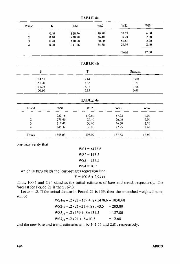
TABLE 4a

Period K WSl ws2 ws3 ws4

1 0.40 920.16 110.80 57.72 6.00

2 0.20 420.88 26.40 39.24 2.00

3 0.20 618.68 30.60 52.68 2.20

4 0.20 341.76 35.20 26.96 2.40

Total 12.60

TABLE 4b

B T Seasonal

104.67 2.64 1.00 151.70 4.45 1.51

196.03 6.13 1.98 100.60 2.85 0.99

TABLE 4c

Period WSI ws2 ws3 ws4

1 920.76 110.80 57.12 6.00 2 279.46 26.40 26.06 2.00 3 312.42 30.60 26.60 2.20 4 345.39 35.20 27.25 2.40

Totals 1858.03 203.00 137.62 12.60

one may verify that WSI = 1478.6

ws2 = 143.5

ws3 = 131.5

ws4 = 10.5

which in turn yields the least-squares regression line

P = 100.6 + 2.94 *t

Thus, 100.6 and 2.94 stand as the initial estimates of base and trend, respectively. The forecast for Period 21 is then 162.3.

Let (Y = .2. If the actual datum in Period 21 is 159, then the smoothed weighted sums will be

WS12,=.2*21*159+.8*1478.6=1850.68

WS2*, = .2*21*21 + .8* 143.5 = 203.00

WS32,=.2*159+.8*131.5 = 137.00

WS42, = .2*21 + .8* 10.5 = 12.60

and the new base and trend estimates will be 10 1.55 and 2.8 1, respectively.

494 APES

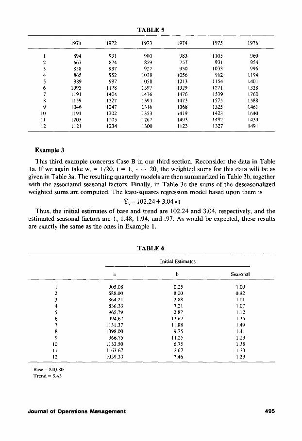
TABLE 5

1971 1972 1973 1974 1975 1976

1 894 931 900 983 1105 960

2 667 874 859 757 931 954

3 858 937 927 950 1033 996

4 865 952 1038 1056 912 1194

5 989 997 1058 1213 1154 1401

6 1093 1178 1397 1329 1271 1328

7 1191 1404 1476 1476 1539 1760

8 1159 1327 1393 1473 1575 1588

9 1046 1247 1316 1368 1325 1461

10 1191 1302 1353 1419 1423 1640

11 1203 1205 1267 1493 1492 1439

12 1121 1234 1300 1123 1327 1491

Example 3

This third example concerns Case B in our third section. Reconsider the data in Table la. Ifwe again take w, = l/20, t = 1, - - - 20, the weighted sums for this data will be as given in Table 3a. The resulting quarterly models are then summarized in Table 3b, together with the associated seasonal factors. Finally, in Table 3c the sums of the deseasonalized weighted sums are computed. The least-squares regression model based upon them is

Yt= 102.24+3.04*t

Thus, the initial estimates of base and trend are 102.24 and 3.04, respectively, and the estimated seasonal factors are 1, 1.48, 1.94, and .97. As would be expected, these results are exactly the same as the ones in Example 1.

TABLE 6

Initial Estimates

a b Seasonal

1 905.08 0.25 1 .oo

2 688.00 8.00 0.92

3 864.21 2.88 1.01

4 836.33 7.2 1 1.07

5 965.79 2.87 1.12

6 994.67 12.67 1.35

7 1131.37 11.88 1.49

8 1098.00 9.75 1.41

9 966.75 11.25 1.29

10 1133.50 6.75 1.38

11 1163.67 2.67 1.33

12 1039.33 7.46 I .29

Base = 810.80

Trend = 5.43

Journal of Operations Management 495

TA

BL

E

7

3e

s9

60

61

b2

4s

64

48s

b‘

b?

‘a I”:

7‘

72

non.

e 9 10

‘1

I2 : 3

:.

‘ 7 m

9

10

‘1

12

‘2‘3

‘S

29

147b

,473

,368

1419

I49S

1123

“OS

931

,033

9‘2

,1

54

1271

1x9

157s

IS25

1423

1492

1327

960

9H

99b

1‘9

4

1401

152m

1760

1 se

e I4

bl

lb40

,439

1491

. .

b (1

, (2

) .-

_

_ __

_ __

-

ems.

57

2.4

2

1.00

0 0.9

0%

762.9

3

O.S

l 1.

000

O.S

Z

073.5

3

2.0

3

1.0

00

@.0

2S

0bS.

07

4.9

0

1.00

0 0.0

21

910.0

3

7.2

0

1.00

0 0.8

19

1085.7

8

b.

16

1.0

00

o.a

i?

lzl:.B

9

b.37

1.

000

0.8

‘4

‘126.0

1

7.9

5

1.00

0 0.8

13

1026.5

9

7.7

1

1.00

0 0.8

11

‘148.6

6

5.9

1

1.00

0 0.

BO

9

1032.4

4

9.S

?

1.0

00

0.0

07

1225.9

0

-1.8

7

1.0

00

0.0

0s

037.9

9

5.1

5

1.00

0 O

.?(r

4

baa

. 72

4.4

3

1.0

00

0.8

29

04L.5

2

3.6

0

1.0

00

0.0

29

994.3

1

-1.0

2

1.0

00

0.8

30

1001.6

5

3.2

2

L.0

00

0.0

SO

1194.9

7

1.7

1

1.0

00

0.8

30

1234.x

l S.6

0

1.0

00

0.

ES

0

1124.

‘a

a.04

1.0

00

0.8

30

1160.2

b

3.2

‘ 1.0

00

0.0

30

1217.9

0

3.6

6

1.0

00

0.0

3,

1147.3

1

b.O

b

1.0

00

0.8

31

97s.

b7

t.

42

1.0

00

0.8

31

992.7

9

-0.

OS

1.0

00

0.9

1b

697.0

3

4.1

7

1.0

00

O.9

1b

909.

as

1.5

4

1.0

00

0.9

20

724.0

0

6.7

4

L.0

00

0.9

25

793.0

1

a.93

1.0

00

0.9

29

1176.5

0

-2.2

6

1.0

00

0.9

3s

1044.6

4

10.3

7

1.0

00

0.9

S8

123‘.

15

5.3

4

1.0

00

0.9

42

104b.b

S

S.8

5

1.0

00

0.9

47

967.4

6

9.3

1

1.0

00

0.9

51

L371.9

0

1.1

9

1.0

00

0.9

55

7b1.9

0

9.9

1

1.0

00

0.9

60

3.9(

?7

0.

VB

B

0.97

8 0.977

0.9

77

0.97

6 0.

976

0.97

5 0.

973

0.9

74

0.9

74

0.9

74

0.9

25

0.9

22

0.9

46

0.9

45

0.9

43

0.9

42

0.9

41

0.9

39

0.9

30

0.9

37

0.9

36

0.9

35

1.0

29

1.0

33

0.9

99

1.0

00

1.0

02

1.0

04

1.0

05

1.0

07

1.0

09

1.0

10

1.0

‘2

1.0

14

_.-

-__

1.05

0 1.

096

1.068

1.0

96

1.0

65

1.09

6 1.0

42

1.0

97

1.0

46

1.1

54

1.0

49

1.1

60

1.0

53

l*lb

b

1.0

56

1.1

72

1.0

%

1.1

70

1.0

62

1.1

83

1.0

66

1.1

09

1.0

69

1,. 1

94

1.0

19

1.1

40

1.0

10

1.1

41

1.0

18

1.1

43

0.9

17

1.1

44

0.9

1‘

1.0

82

0.9

05

1.0

79

0.

a99

L.0

77

0.8

93

1.0

73

0.8

07

1.0

72

0.0

81

1.0

70

0.0

76

1.O

t.S

0.0

70

1.0

65

0.9

ZS

1.1

72

0.9

52

1.1

73

0.9

91

1.1

79

i.00a

1.1

02

1.0

95

1.2

03

1.

LO

2

1.2

93

1,1

09

1.3

02

1.1

16

1.1

12

1.1

2’3

1.3

21

1.1

31

1.3

30

1.1

38

1.3

40

1.1

41

1.3

49

(61

(7)

___

_-_

1.33

, 1.

466

1.3

52

1.4

79

1.36

6 1.4

92

1.30

0 1.3

05

1.3

94

1.5

17

1.3

17

1.5

20

1.3

21

1.4

b2

L.3

25

1.4

66

1.3

29

1.4

70

1.3

33

1.4

73

1.3

3,

1.4

77

1.3

40

1.4

00

I.278

1.4

11

1.2

77

1.4

10

1.2

77

1.4

09

I.276

1.4

08

1.2

76

1.4

07

1,2

01

1.4

06

t.201

1.3

93

1.1

97

1.3

91

1.1

92

1.3

90

l.lB

0

1.3

00

1.1

84

1.3

07

1.1

79

1.3

85

1.2

95

1.5

25

1.2

97

1.5

31

1.2

99

1.5

3,

1.3

01

1.5

43

1.3

03

1.5

49

1.3

13

‘.3X

1.3

13

1.&

S?

1.3

18

1.6

48

1.3

20

1.6

59

1.3

23

1.6

70

1.3

21

1.6

00

1.3

2,

l.L91

SO

.901

(9)

1.3

85

1.3

95

1.4

05

i.414

I.424

1.4

33

1.4

41

1.4

24

1.4

30

1.4

36

1.4

41

1.4

47

1.3

81

1.3

02

1.3

03

1.3

04

1.3

0%

1.3

85

1.3

06

1.3

89

1.3

09

1.3

90

1.3

91

1.3

92

l.JSS

1.5

44

1.5

53

l.St.

1

1.5

70

i.5?0

1.5

87

1.5

54

1.5

59

1.5

65

1.5

71

1.5

76

1.2

76

1.2

89

1.3

02

1.3

14

1.3

26

1.3

37

1.3

40

1.3

59

1.3

18

1.3

24

1.3

30

1.3

36

1.2

75

1.2

76

1.2

78

1.2

79

1.2

00

1.2

01

1.2

03

1.2

04

1.2

20

1.2

17

1.2

14

1.2

11

1.3

31

1.3

35

1.3

38

1.3

42

1.3

45

1.3

49

1.3

52

l.SSb

1.3

90

1.4

04

1.4

10

1.4

16

--__

1.3

58

1.36

4 1.

369

1.3

74

li

379

1.3

84

1.3

89

1.3

94

I.390

1.3

90

1.3

93

1.3

96

1.3

31

1.3

29

1.3

28

1.3

2,

1.3

26

l.S25

I.324

1.3

23

1.3

23

1.2

9,

1.2

00

1.2

85

1.4

13

1.4

1,

1.4

21

1.4

25

1.4

29

1.4

33

1.4

s,

1.4

4‘

1.4

45

1.5

29

I.SS9

1.5

48

1.30

3 I.

SO

2

l.SO

2

1.3

01

1.3

00

1.2

99

1.2

99

I.298

1.2

90

L.2

97

1.4

00

1.4

00

1.3

46

1.3

49

1.3

52

1.3

34

1.3

57

1.3

60

i.363

1.3

65

1.3

60

1.3

71

1.3

26

1.3

2b

1.4

60

1.4

67

1.4

73

1.4

80

1.4

06

1.4

93

1.4

99

1.5

0s

1.5

12

1.5

10

1.4

se

1.4

59

(I2,

Bas

e __

--

-we-

1.2

73

020.0

0

1.2

00

049.6

4

1.2

07

849.9

s 1.2

93

846.8

7

1.2

99

832.2

5

1.3

05

ass.

97

l.S‘l

039.0

3

1.3

17

8Sb.7

1

1.3

23

83b.

65

1.5

20

036.9

s 1.5

34

024.9

7

1.1

97

844.5

9

1.1

53

875.1

4

1.1

24

057.3

9

‘.‘lb

WSS.S

8

1.1

07

00S.2

7

1.0

99

094.4

9

1.0

91

900.5

9

1.0

83

900.8

5

1.0

75

904.4

0

1.0

60

916.1

3

1.0

60

923.6

0

l.O

SS

920.2

7

1.1

39

913.0

9

1.2

55

060.9

0

1.2

b‘

855.0

7

1.2

67

014.9

7

1.2

73

823.

ii

1.2

78

794.1

8

1.2

84

797.2

0

1.2

90

776.0

8

1.2

96

702.3

9

1.5

01

773.2

2

l.SO

?

752.7

1

1.5

‘3

771.6

1

1.3

70

748.

‘3

Trln

d F

OP

-.E

..t

5.08

3.7

9

3.5

9

3.7

5

4.3

1

4.1

7

4.0

5

4.1

3

4.1

5

4.0

7

4.3

9

3.6

2

4.1

2

4.5

9

4.67

s.

as

3.64

3.

33

3.40

S

.61

3.38

3.2

0

S.2

b

s.

b2

2.6

5

2.7

3

2.4

, 3.2

2

3.7

s 3.3

6

3.8

0

3.7

‘ 3.0

0

4.0

9

S.b

b

4.0

2

927.1

9

9as

. 2B

1050.0

5

1097.6

1

14‘2

.21

lss‘

.aI

146S.E

l 1309.0

6

‘436.4

1

1133.

JS

1381.6

1

102L.7

5

025.6

7

1001.6

5

11‘6

.22

1244.1

5

1391.9

5

1534.6

6

1524.0

6

142s*

42

1471.8

1

lS30.7

5

‘iaS

.74

1133.6

3

937.8

6

1060.3

4

972.9

9

1220.4

1

1365.3

0

1610.3

7

1651.8

5

1407.b

9

1500.9

9

LJ03.9

0

lSS9.0

3

‘041.9

0

The forecast for Period 2 1 is again 166.1. Suppose that the actual datum for Period 2 1 is 159. Then the smoothed weights and weighted sums will be as summarized in Table 4a. For example,

WS12i=.2*21*159+.8*316.20=920.76

WS22, = .8 * 526.10 = 420.88

WS321 = .8 *773.35 = 618.68

WS42, = .8 * 427.20 = 341.76

The new quarterly models and seasonal factors are given in Table 4b and the new sums of deseasonalized weighted sums in Table 4c, yielding the regression model

Yt= 102.31+2.80*t

Thus, the updated estimates of base and trend are 102.3 1 and 2.80, respectively, and the new seasonal factors are 1 .OO, 1.5 1, 1.98, and .99.

Example 4

This final example analyzes six years of monthly data on motorcycle registrations. The data, taken from Makridakis, Wheelwright, and McGee [2, pp. 138-391, is reproduced in Table 5.

The first three years of data will be used to generate initial estimates of the parameters as described in the second section. These estimates will then be updated by applying the exponential smoothing principle to incorporate each new month of data from the last three years. The initial estimates appear in Table 6. They were generated using simple regression analysis for the monthly models, with equal weights applied to all years.

Computational results for Periods 37 to 72 are given in Table 7. The actual datum for each period appears in the third column, with the resulting updated parameter estimates in the columns that follow it. Thus, for example, 885.57 and 2.42 are the new parameter estimates for the Month 1 regression model, and 828.00 and 5.08 are the new estimates of underlying base and trend. The forecast for the next period is the last element in each row. In all the computations, CY = .083333, simply following the rule of thumb of choosing the smoothing constant as the reciprocal of the number of periods in one seasonal cycle.

Journal of Operations Management 497