1-s2.0-S0196890403002425-main

8/12/2019 1-s2.0-S0196890403002425-main

http://slidepdf.com/reader/full/1-s20-s0196890403002425-main 1/7

Global solar radiation estimation using sunshine

duration in Spain

J. Almorox *, C. Hontoria

Departamento de Edafolog ıa, Escuela T ecnica Superior de Ingenieros Agronomos, Universidad Politecnica de Madrid,

Avd. Complutense s/n, 28040 Madrid, Spain

Received 17 April 2003; accepted 19 August 2003

Abstract

Several equations were employed to estimate global solar radiation from sunshine hours for 16 mete-

orological stations in Spain, using only the relative duration of sunshine. These equations included the

original Angstr€om–Prescott linear regression and modified functions (quadratic, third degree, logarithmic

and exponential functions). Estimated values were compared with measured values in terms of the coeffi-

cient of determination, standard error of the estimate and mean absolute error. All the models fitted the

data adequately and can be used to estimate global solar radiation from sunshine hours. This study finds

that the third degree models performed better than the other models, but the linear model is preferred due

to its greater simplicity and wider application. It is also found that seasonal partitioning does not signifi-

cantly improve the estimation of global radiation.

2003 Elsevier Ltd. All rights reserved.

Keywords: Angstr€om equation; Global solar radiation estimation; Sunshine duration; Correlation models

1. Introduction

Knowledge of local solar radiation is essential for many applications, including architecturaldesign, solar energy systems and particularly for design methods, crop growth models andevapotranspiration estimates in the design of irrigation systems. In spite of the importance of solar radiation measurements, this information is not readily available due to the cost and

maintenance and calibration requirements of the measuring equipment. The limited coverage of radiation values dictates the need to develop models to estimate solar radiation based on other,

Energy Conversion and Management 45 (2004) 1529–1535

www.elsevier.com/locate/enconman

* Corresponding author. Tel.: +34-91-3365-689; fax: +34-91-3365-680.

E-mail address: [email protected] (J. Almorox).

0196-8904/$ - see front matter

2003 Elsevier Ltd. All rights reserved.doi:10.1016/j.enconman.2003.08.022

http://mail%20to:%[email protected]/

http://mail%20to:%[email protected]/

8/12/2019 1-s2.0-S0196890403002425-main


more readily available, data [1]. Several empirical models have been used to calculate solar ra-

diation, using variables such as sunshine hours [2], air temperature [3], precipitation [4], relativehumidity [5] and cloudiness [6]. The most commonly used parameter for estimating global solar

radiation is sunshine duration. Sunshine duration can be easily and reliably measured and dataare widely available. Most of the models for estimating solar radiation that appear in the liter-ature use the sunshine ratio [1]. The most widely used method is that of Angstr€om [2], whoproposed a linear relationship between the ratio of average daily global radiation to the corre-

sponding value on a completely clear day and the ratio of average daily sunshine duration to themaximum possible sunshine duration. The problem of determining clear sky global irradiance wasbypassed by Prescott, who suggested using extraterrestrial radiation intensity values instead.

Prescott [7] put the equation in a more convenient form by replacing the average global radiationon a clear day with the extraterrestrial radiation.

The objective of this study was to validate several expression models for the prediction of monthly average daily global radiation on a horizontal surface from sunshine hours and to select

the most adequate model.

2. Materials and methods

The Angstr€om–Prescott formula is

H = H 0 ¼ a þ bðn= N Þ ð1Þ

where H and H 0 are, respectively, the monthly mean daily global radiation and the daily extra-

terrestrial radiation on a horizontal surface; n and N are, respectively, the monthly average dailysunshine duration and the monthly average maximum possible daily sunshine duration; and a andb are empirically determined regression constants.

The sky is overcast when the ratio n= N is zero, so the regression coefficient ‘‘a’’ is a measure of the overall atmospheric transmission for total cloud conditions, while the term ‘‘b’’ is the rate of increase of H = H 0 with n= N . The sum ða þ bÞ denotes the overall atmospheric transmission underclear sky conditions. The mean transmission has a typical factor value of around 0.75 [8]. These

constants can assume a wide range of values, depending on the location considered, and can beinferred from correlations established at neighboring locations. Thus, for example, when using theFAO 56 Penman estimation method [9], Angstr€om values calibration is recommended. Variations

in the a and b values are explained as a consequence of local and seasonal changes in the type andthickness of cloud cover, the effects of snow covered surfaces, the concentrations of pollutants and

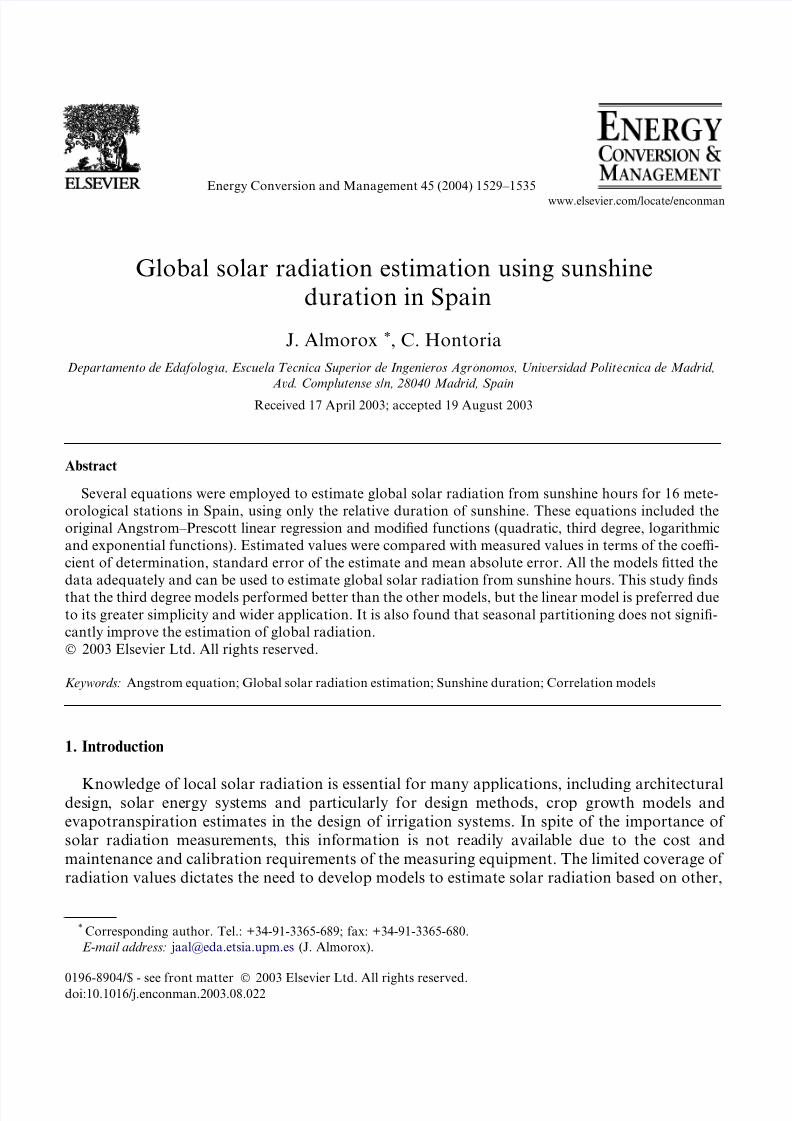
latitude [8,10].Several types of regression models have been proposed in the literature for estimating global

solar radiation from extraterrestrial irradiance and measured and theoretical daily sunshineduration (Table 1).

The daily extraterrestrial radiation on a horizontal surface at the middle of the month can be

calculated as a function of the solar constant (G sc), the eccentricity correction factor of the Earthsorbit ( E 0), the latitude of the site (U), the solar declination (d) and the mean sunrise hour angle(w s) in MJm2 day1 using the following equation:

1530 J. Almorox, C. Hontoria / Energy Conversion and Management 45 (2004) 1529–1535

8/12/2019 1-s2.0-S0196890403002425-main


H 0 ¼ ð1=pÞ G sc E 0 ðcosU cos d sinws þ ðp=180Þ sinU sin d wsÞ ð2Þ

The solar constant is the amount of energy received at the top of the Earths atmosphere,measured at an average distance between the Earth and Sun on a surface oriented perpendicular

to the Sun. The generally accepted solar constant of 1367 W m2 (an equivalent daily value of 118.108 MJ m2 day1 to reconcile units) is a satellite measured yearly average.

The eccentricity correction factor can be calculated by the expression [14]:

E 0 ¼ 1:00011 þ 0:034221 cos C þ 0:00128 sin C þ 0:000719 cos 2C þ 0:000077 sin 2C

ð3Þ

The solar declination d can be computed in degrees from the equation [14]:

d ¼ ð180=pÞ ð0:006918 0:399912 cos C þ 0:070257 sin C 0:006758 cos 2C

þ 0:000907 sin 2C 0:002697 cos 3C þ 0:00148 sin 3CÞ ð4Þ

where C ¼ 2p ðn 1Þ=365 (radians) and n is the number of the day of the year, starting from the

first of January.The geometric mean sunrise hour angle for the month on a horizontal surface can be calculated

(except in the absence of sunrise and sunset, during the polar day and night) in degrees from:

ws ¼ cos1ð tanU tan dÞ ð5Þ

The maximum possible number of daylight hours is given by:

N ¼ ð2=15Þ ws ð6Þ

The main purpose of this work was to obtain sets of regression constants for five different re-gression models for as many weather stations as possible with data available in Spain. To this end,

we employed the measured data of monthly average global solar radiation on horizontal surfacesand sunshine hours from 16 meteorological stations across Spain, given in Table 2, to generate the

equations. The data were obtained from the National Meteorological Institute (Ministerio deMedio Ambiente, Spain).

Five different regression models were applied, four proposed in the literature (linear, quadratic,

polynomial third degree and logarithmic) and an exponential model used in this work. Coefficientvalues were calculated from regression analysis between H = H 0 and n= N for a long period and eachmonth. This method is considered by Tadros [15] as the best for predicting global solar radiation

over eight meteorological stations in Egypt. To determine the annual regressions, we used datafrom all months of the year. Since coefficients vary from season to season [16,17], the data was

Table 1

Regression models proposed in the literature

Models Regression equations Source

Linear H = H 0 ¼ a þ b ðn= N Þ Angstr€om–Prescott [2,7]

Quadratic H = H 0 ¼ a þ b ðn= N Þ þ c ðn= N Þ2Akinoglu and Ecevit [11]

Third degree H = H 0 ¼ a þ b ðn= N Þ þ c ðn= N Þ2 þ d ðn= N Þ3Ertekin and Yaldiz [12]

Logarithmic H = H 0 ¼ a þ b logðn= N Þ Ampratwum and Dorvlo [13]

J. Almorox, C. Hontoria / Energy Conversion and Management 45 (2004) 1529–1535 1531

8/12/2019 1-s2.0-S0196890403002425-main


separated into the summer (June, July, August), autumn (September, October, November), spring(March, April, May) and winter (December, January, February) seasons.

The regression models were developed to find the best predictive equation using Statgraphics

Plus (version 5) software. The accuracy of the estimated values was tested by calculating the R-squared statistic, the standard error of estimate and the mean absolute error. The R-squared

statistic indicates the percentage of variability of the dependent variable as it was fitted in the fullmodel. The standard error of the estimate shows the value for the standard deviation of the re-siduals, estimated by the square root of the mean squared error. The mean absolute error is a

measure of the forecast accuracy, calculated by summing the absolute errors and dividing by thenumber of observations. The square root of the mean squared error and the mean absolute error

are the fundamental measures of accuracy [18].

3. Results and discussion

The equations developed and the R2, SEE and MAE values of the equations are given in Tables3 and 4. The model results for annual data are listed in Table 3, and the results of the regressionanalyses for winter, spring, summer and autumn can be seen in Table 4.

Comparing the results, we can see that all the regression equations gave very good results. Thequadratic model and the third degree equation gave the best estimate and have the smallest errorsfor the annual and seasonal values. The logarithmic and exponential models performed worse

than the other models, giving the largest standard error of the estimate and mean absolute error.The linear, second and third degree regression equations gave good, and very similar, accuracy.Given the small differences between the variance explained by linear regression and the most

Table 2

Geographical location and period of data of the meteorological stations used

Station Latitude (N) Longitude Elevation (m) Period of observation

Badajoz 38 53 0 0000

6 49 0 4500

W 185 1976–1984Bilbao 43 17 0 53

002 54 0 21

00W 39 1985–2000

Caceres 39 28 0 2000

6 20 0 2200

W 405 1983–2000

Cadiz 36 29 0 5500

6 15 0 3700

W 8 1991–2000

Castellon 39 57 0 0000

0 01 0 0000

W 35 1984–1991

La Coru~na 43 22 0 0200

8 25 0 1000

W 58 1985–2000

Logro~no 42 27 0 5000

2 22 0 4700

W 364 1983–1998

Madrid 40 27 0 1000

3 43 0 2700

W 664 1976–1999

Murcia 38 00 0 1000

1 10 0 1000

W 62 1985–2000

Oviedo 43 21 0 1300

5 52 0 2400

W 336 1981–1999

San Sebastian 43 18 0 2400

2 02 0 2200

W 259 1983–2000

Santander 43 27 0 5300

3 49 0 0800

W 64 1983–1998

Sevilla 37 25 0 1500

5 53 0 4700

W 34 1981–1988

Toledo 39 53 0 0500

4 02 0 5800

W 516 1983–1998

Tortosa 40 49 0 1400

0 29 0 2900

E 48 1980–1998

Valladolid 41 42 0 0000

4 51 0 0000

W 846 1982–1998

Source: Ministerio de Medio Ambiente, Spain.


8/12/2019 1-s2.0-S0196890403002425-main


accurate equation, the third degree one (86.4% and 86.5%, for the annual model), and the sim-

plicity and wider application of the linear equation, the simple linear regression, is in practice,sufficient, and the use of the quadratic and third degree equations is not sufficiently justified.

Table 3

Annual regression results, and R2, SEE, and MAE values of models

Equations R2 SEE MAE

Annual Linear H = H 0 ¼ 0:2170 þ 0:5453 ðn= N Þ 0.864 0.0361 0.0271

Quadratic H = H 0 ¼ 0:1840 þ 0:6792 ðn= N Þ 0:1228 ðn= N Þ20.865 0.0359 0.0270

Third degree H = H 0 ¼ 0:230 þ 0:3809 ðn= N Þ þ 0:4694 ðn= N Þ2 0:3657 ðn= N Þ30.865 0.0359 0.0269

Logarithmic H = H 0 ¼ 0:6902 þ 0:6142 logðn= N Þ 0.842 0.0388 0.0298

Exponential H = H 0 ¼ 0:0271 þ 0:3096 eðn= N Þ 0.851 0.0378 0.0286

R2 ( R-squared): coefficient of determination.

SEE: standard error of the estimate.

MAE: mean absolute error.

Table 4

Regression results for winter, spring, summer and autumn, and R

2

( R-squared), SEE (standard error of the estimate),and MAE (mean absolute error) values

Equations R2 SEE MAE

Winter

Linear H = H 0 ¼ 0:2114 þ 0:5291 ðn= N Þ 0.865 0.0314 0.0235





Spring

Linear H = H 0 ¼ 0:2414 þ 0:5375 ðn= N Þ 0.825 0.0351 0.0250

Quadratic H = H 0 ¼ 0:2216 þ 0:6188 ðn= N Þ 0:0773 ðn= N Þ2 0.826 0.0351 0.0249Third degree H = H 0 ¼ 0:2306 þ 0:5590 ðn= N Þ þ 0:0455 ðn= N Þ2 0:0792 ðn= N Þ3

0.826 0.0351 0.0249



Summer

Linear H = H 0 ¼ 0:2518 þ 0:5004 ðn= N Þ 0.876 0.0334 0.0246





AutumnLinear H = H 0 ¼ 0:1966 þ 0:5580 ðn= N Þ 0.870 0.0318 0.0235


Third degree H = H 0 ¼ 0:2733 0:0063 ðn= N Þ þ 1:2665 ðn= N Þ2 0:8793 ðn= N Þ30.872 0.0316 0.0234




8/12/2019 1-s2.0-S0196890403002425-main


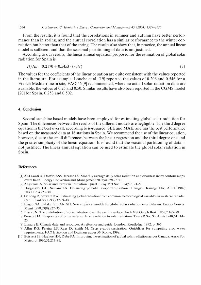
From the results, it is found that the correlations in summer and autumn have better perfor-

mance than in spring, and the annual correlation has a similar performance to the winter cor-relation but better than that of the spring. The results also show that, in practice, the annual linear

model is sufficient and that the seasonal partitioning of data is not justified.According to our results, the linear annual equation proposed for the estimation of global solar

radiation for Spain is

H = H 0 ¼ 0:2170 þ 0:5453 ðn= N Þ ð7Þ

The values for the coefficients of the linear equation are quite consistent with the values reportedin the literature. For example, Louche et al. [19] reported the values of 0.206 and 0.546 for a

French Mediterranean site; FAO 56 [9] recommended, where no actual solar radiation data areavailable, the values of 0.25 and 0.50. Similar results have also been reported in the CGMS model[20] for Spain, 0.253 and 0.502.

4. Conclusion

Several sunshine based models have been employed for estimating global solar radiation forSpain. The differences between the results of the different models are negligible. The third degree

equation is the best overall, according to R-squared, SEE and MAE, and has the best performancebased on the measured data at 16 stations in Spain. We recommend the use of the linear equation,

however, due to the small differences between the linear regression and the third degree one andthe greater simplicity of the linear equation. It is found that the seasonal partitioning of data isnot justified. The linear annual equation can be used to estimate the global solar radiation in

Spain.

References

[1] Al-Lawati A, Dorvlo ASS, Jervase JA. Monthly average daily solar radiation and clearness index contour maps

over Oman. Energy Conversion and Management 2003;44:691–705.

[2] Angstr€om A. Solar and terrestrial radiation. Quart J Roy Met Soc 1924;50:121–5.

[3] Hargreaves GH, Samani ZA. Estimating potential evapotranspiration. J Irrigat Drainage Div, ASCE 1982;

108(1 IR3):223–30.

[4] De Jong R, Stewart DW. Estimating global radiation from common meteorological variables in western Canada.

Can J Plant Sci 1993;73:509–18.[5] Elagib NA, Babiker SF, Alvi SH. New empirical models for global solar radiation over Bahrain. Energy Conver

Mgmt 1998;39(8):827–35.

[6] Black JN. The distribution of solar radiation over the earths surface. Arch Met Geoph Biokl 1956;7:165–89.

[7] Prescott JA. Evaporation from a water surface in relation to solar radiation. Trans R Soc Sci Austr 1940;64:114–

25.

[8] Linacre E. Climate data and resources. A reference and guide. London: Routledge; 1992. p. 366.

[9] Allen RG, Pereira LS, Raes D, Smith M. Crop evapotranspiration. Guidelines for computing crop water

requirements. FAO Irrigation and Drainage paper 56. Rome, 1998.

[10] Boisvert JB, Hayhoe HN, Dube PA. Improving the estimation of global solar radiation across Canada. Agric For

Meteorol 1990;52:275–86.


8/12/2019 1-s2.0-S0196890403002425-main


[11] Akinoglu BG, Ecevit A. Construction of a quadratic model using modified Angstr€om coefficients to estimate global

solar radiation. Solar Energy 1990;45:85–92.

[12] Ertekin C, Yaldiz O. Comparison of some existing models for estimating global solar radiation for Antalya

(Turkey). Energy Convers Mgmt 2000;41:311–30.

[13] Ampratwum DB, Dorvlo ASS. Estimation of solar radiation from the number of sunshine hours. Appl Energy

1990;62:161–7.

[14] Spencer JW. Fourier series representation of the position of the Sun. Search 1971;2(5):172.

[15] Tadros MTY. Uses of sunshine duration to estimate the global solar radiation over eight meteorological stations in

Egypt. Renew Energy 2000;21:231–46.

[16] Hussain M, Rahman L, Rahman MM. Techniques to obtain improved predictions of global radiation from

sunshine duration. Renew Energy 1999;18:263–75.

[17] Togrul IT, Togrul H, Evin D. Estimation of monthly global solar radiation from sunshine duration measurement

in Elazig. Renew Energy 2000;19:587–95.

[18] Chegaar M, Chibani A. Global solar radiation estimation in Algeria. Energy Conver Mgmt 2001;42:967–73.

[19] Louche A, Notton G, Poggi P, Simonnot G. Correlations for direct normal and global horizontal irradiations on a

French Mediterranean site. Solar Energy 1991;46(4):261–6.

[20] Supit I, Van der Goot E, editors. Updated system description of the WOFOST crop growth simulation model asimplemented in the crop growth monitoring system applied by the European Commission. Internet On-line Book.

Trebook 7. Heelsum, The Netherlands: Treemail Publishers; 2003.


1-s2.0-S0196890403002425-main

Documents

Transcript of 1-s2.0-S0196890403002425-main