1-s2.0-S0098135415000502-main
22
Computers and Chemical Engineering 79 (2015) 113–134 Contents lists available at ScienceDirect Computers and Chemical Engineering j ourna l ho me pa g e: www.elsevier.com/locate/compchemeng Planning and scheduling of steel plates production. Part I: Estimation of production times via hybrid Bayesian networks for large domain of discrete variables Junichi Mori, Vladimir Mahalec ∗ Department of Chemical Engineering, McMaster University, Hamilton, Ontario, Canada L8S 4L7 a r t i c l e i n f o Article history: Received 4 June 2014 Received in revised form 4 February 2015 Accepted 8 February 2015 Available online 5 March 2015 Keywords: Estimation of production time Hybrid Bayesian network Structure learning Large domain of discrete variables Decision tree Steel plate production a b s t r a c t Knowledge of the production loads and production times is an essential ingredient for making successful production plans and schedules. In steel production, the production loads and the production times are impacted by many uncertainties, which necessitates their prediction via stochastic models. In order to avoid having separate prediction models for planning and for scheduling, it is helpful to develop a single prediction model that allows us to predict both production loads and production times. In this work, Bayesian network models are employed to predict the probability distributions of these variables. First, network structure is identified by maximizing the Bayesian scores that include the likelihood and model complexity. In order to handle large domain of discrete variables, a novel decision-tree structured conditional probability table based Bayesian inference algorithm is developed. We present results for real- world steel production data and show that the proposed models can accurately predict the probability distributions. © 2015 Elsevier Ltd. All rights reserved. 1. Introduction Accurate estimation of the production loads and the total pro- duction times in manufacturing processes is crucial for optimal operations of real world industrial systems. In this paper, a produc- tion load represents the number of times that a product is processed in the corresponding process unit and a production time is defined as the length of time from production start to completion. Produc- tion planning and scheduling for short, medium and long term time horizons employ various optimization models and algorithms that require accurate knowledge of production loads and total produc- tion times from information at each of the processing steps. The approaches to predict the production loads and total production times can be either based on mechanistic model or can employ data-driven techniques. Model-based prediction methods may be applied only if accurate mechanistic models of the processes can be developed. First principal models require in-depth knowledge of the processes and still cannot take into consideration all uncer- tainties that exist in the processes. Therefore, mechanistic models may not work well for prediction of production loads and produc- tion times of the real-world industrial processes. On the other hand, ∗ Corresponding author. Tel.: +1 905 525 9140. E-mail address: [email protected] (V. Mahalec). data-driven approaches do not require in-depth process knowl- edge and some advanced techniques can deal with the process uncertainties. The most straightforward approach is to use the classical sta- tistical models (e.g. regression models) that estimate the values of new production loads and a production time from the past values in the historical process data. The relationships between the targeted variables and other relevant variables are used to compute the sta- tistical model that can predict the production loads and production times. However, such models are too simple to predict the nonlin- ear behavior and estimate the system uncertainties. An alternative simple method is to compute the average of these values per each production group that has similar production properties and then utilize the average values of each production group as the predic- tion (Ashayeria et al., 2006). In this case the prediction accuracy significantly depends on the rules that govern creation of produc- tion groups and it may be challenging to find the appropriate rules from process knowledge only. To overcome this limitation, super- vised classification techniques such as artificial neural networks (ANN), support vector machine, Fisher discriminant analysis and K-nearest neighbors (KNN) may be useful to design the rules to make production groups from historical process data. However, even though we can accurately classify the historical process data into an appropriate number of production groups, these methods do not consider model uncertainties and cannot handle missing http://dx.doi.org/10.1016/j.compchemeng.2015.02.005 0098-1354/© 2015 Elsevier Ltd. All rights reserved.
description
a seminar topic
Transcript of 1-s2.0-S0098135415000502-main
Pod
JD
a
ARRAA
KEHSLDS
1
dotiathrtatdabotmt
h0
Computers and Chemical Engineering 79 (2015) 113–134
Contents lists available at ScienceDirect
Computers and Chemical Engineering
j ourna l ho me pa g e: www.elsev ier .com/ locate /compchemeng
lanning and scheduling of steel plates production. Part I: Estimationf production times via hybrid Bayesian networks for large domain ofiscrete variables
unichi Mori, Vladimir Mahalec ∗
epartment of Chemical Engineering, McMaster University, Hamilton, Ontario, Canada L8S 4L7
r t i c l e i n f o
rticle history:eceived 4 June 2014eceived in revised form 4 February 2015ccepted 8 February 2015vailable online 5 March 2015
eywords:
a b s t r a c t
Knowledge of the production loads and production times is an essential ingredient for making successfulproduction plans and schedules. In steel production, the production loads and the production timesare impacted by many uncertainties, which necessitates their prediction via stochastic models. In orderto avoid having separate prediction models for planning and for scheduling, it is helpful to develop asingle prediction model that allows us to predict both production loads and production times. In thiswork, Bayesian network models are employed to predict the probability distributions of these variables.
stimation of production timeybrid Bayesian networktructure learningarge domain of discrete variablesecision treeteel plate production
First, network structure is identified by maximizing the Bayesian scores that include the likelihood andmodel complexity. In order to handle large domain of discrete variables, a novel decision-tree structuredconditional probability table based Bayesian inference algorithm is developed. We present results for real-world steel production data and show that the proposed models can accurately predict the probabilitydistributions.
© 2015 Elsevier Ltd. All rights reserved.
. Introduction
Accurate estimation of the production loads and the total pro-uction times in manufacturing processes is crucial for optimalperations of real world industrial systems. In this paper, a produc-ion load represents the number of times that a product is processedn the corresponding process unit and a production time is defineds the length of time from production start to completion. Produc-ion planning and scheduling for short, medium and long term timeorizons employ various optimization models and algorithms thatequire accurate knowledge of production loads and total produc-ion times from information at each of the processing steps. Thepproaches to predict the production loads and total productionimes can be either based on mechanistic model or can employata-driven techniques. Model-based prediction methods may bepplied only if accurate mechanistic models of the processes cane developed. First principal models require in-depth knowledgef the processes and still cannot take into consideration all uncer-
ainties that exist in the processes. Therefore, mechanistic modelsay not work well for prediction of production loads and produc-ion times of the real-world industrial processes. On the other hand,
∗ Corresponding author. Tel.: +1 905 525 9140.E-mail address: [email protected] (V. Mahalec).
ttp://dx.doi.org/10.1016/j.compchemeng.2015.02.005098-1354/© 2015 Elsevier Ltd. All rights reserved.
data-driven approaches do not require in-depth process knowl-edge and some advanced techniques can deal with the processuncertainties.
The most straightforward approach is to use the classical sta-tistical models (e.g. regression models) that estimate the values ofnew production loads and a production time from the past values inthe historical process data. The relationships between the targetedvariables and other relevant variables are used to compute the sta-tistical model that can predict the production loads and productiontimes. However, such models are too simple to predict the nonlin-ear behavior and estimate the system uncertainties. An alternativesimple method is to compute the average of these values per eachproduction group that has similar production properties and thenutilize the average values of each production group as the predic-tion (Ashayeria et al., 2006). In this case the prediction accuracysignificantly depends on the rules that govern creation of produc-tion groups and it may be challenging to find the appropriate rulesfrom process knowledge only. To overcome this limitation, super-vised classification techniques such as artificial neural networks(ANN), support vector machine, Fisher discriminant analysis andK-nearest neighbors (KNN) may be useful to design the rules to
make production groups from historical process data. However,even though we can accurately classify the historical process datainto an appropriate number of production groups, these methodsdo not consider model uncertainties and cannot handle missing
1 Chem
vfpm
gparbnpTbrs
difthtrr1if(bcddovTci2ssvcaiboEtdbcebsdb
tmthtie1
14 J. Mori, V. Mahalec / Computers and
alues and unobserved variables. In addition, we are typicallyorced to have multiple specific models tailored for specific pur-oses, e.g. for production planning or for scheduling, which causesodel maintenance issues and lack of model consistency.Bayesian network (BN) models offer advantages of having a sin-
le prediction model for predicting the production loads and totalrocess times in planning and scheduling. Bayesian networks arelso called directed graphical models where the links of the graphsepresent direct dependence among the variables and are describedy arrows between links (Pearl, 1988; Bishop, 2006). Bayesianetwork models are popular for representing conditional inde-endencies among random variables under system uncertainty.hey are popular in the machine learning communities and haveeen applied to various fields including medical diagnostics, speechecognition, gene modeling, cancer classification, target tracking,ensor validation, and reliability analysis.
The most common representations of conditional probabilityistributions (CPDs) at each node in BNs are conditional probabil-
ty tables (CPTs), which specify marginal probability distributionsor each combination of values of its discrete parent nodes. Sincehe real industrial plant data often include discrete variables whichave large discrete domains, the number of parameters becomesoo large to represent the relationships by the CPTs. In order toeduce the number of parameters, context-specific independenceepresentations are useful to describe the CPTs (Boutilier et al.,996). Efficient inference algorithm that exploits context-specified
ndependence (Poole and Zhang, 2003) and the learning methodsor identification of parameters of context-specific independenceFriedman and Goldszmidt, 1996; Chickering et al., 1997) haveeen developed. The restriction of these methods is that all dis-rete values must be already grouped at an appropriate level ofomain size since learning structured CPTs is NP-hard. However,iscrete process variables typically have large domains and the taskf identifying a reasonable set of groups that distinguish well thealues of discrete variables requires in-depth process knowledge.o overcome this limitation, attribute – value hierarchies (AVHs) thatapture meaningful groupings of values in a particular domain arentegrated with the tree-structured CPTs (DesJardins and Rathod,008). Such approach is not applicable in general process systems,ince some discrete process variables do not contain hierarchaltructures and thus AVHs cannot capture the useful abstracts ofalues in that domain. In addition, this model cannot handle theontinuous variables without discretizing them. Furthermore, theuthors do not describe how to apply AVH-derived CPTs to Bayesiannference. Therefore, this method has difficulty predicting proba-ility distributions of production loads and total process time frombserved process variables in the real-world industrial processes.fficient alternative inference methods in Bayesian Networks con-aining CPTs that are represented as decision trees have beeneveloped (Sharma and Poole, 2003). The inference algorithm isased on variable elimination (VE) algorithm. However, because theomputational complexity of the exact inference such as VE growsxponentially with the size of the network, this method may note appropriate for Bayesian networks for large scale industrial dataets. In addition, the method does not deal with application of theecision-tree structured CPTs to hybrid Bayesian networks, whereoth discrete and continuous variables appear simultaneously.
In hybrid Bayesian networks, the most commonly used modelhat allows exact inference is the conditional linear Gaussian (CLG)
odel (Lauritzen, 1992; Lauritzen and Jensen, 2001). However,he proposed network model does not allow discrete variables toave continuous parents. To overcome this limitation, the CPDs of
hese nodes are typically modeled as softmax function, but theres no exact inference algorithm. Although an approximate infer-nce via Monte Carlo method has been proposed (Koller et al.,999), the convergence can be quite slow in Bayesian Networksical Engineering 79 (2015) 113–134
with large domain of discrete variables. Another approach is to dis-cretize all continuous variables in a network and treat them as ifthey are discrete (Kozlov and Koller, 1997). Nevertheless, it is typ-ically impossible to discretize the continuous variables as finelyas needed to obtain reasonable solutions and the discretizationleads to a trade-off between accuracy of the approximation andcost of computation. As another alternative, the mixture of trun-cated exponential (MTE) model has been introduced to handle thehybrid Bayesian networks (Moral et al., 2001; Rumi and Salmeron,2007; Cobb et al., 2007). MTE models approximate arbitrary prob-ability distribution functions (PDFs) using exponential terms andallow implementation of inference in hybrid Bayesian networks.The main advantage of this method is that standard propagationalgorithms can be used. However, since the number of regres-sion coefficients in exponential functions linearly grows with thedomain size of discrete variables, MTE model may not work wellfor the large Bayesian networks that are required to represent theindustrial processes.
Production planning and scheduling in the steel industry arerecognized as challenging problems. In particular, the steel plateproduction is one of the most complicated processes because steelplates are high-variety low-volume products manufactured onorder and they are used in many different applications. Althoughthere have been several studies on scheduling and planning prob-lems in steel production, such as continuous casting (Tang et al.,2000; Santos et al., 2003), smelting process (Harjunkoski andGrossmann, 2001) and batch annealing (Moon and Hrymak, 1999),few studies have dealt with steel plate production scheduling. Steelrolling processes manufacture various size of plates from a widerange of materials. Then, at the finishing and inspection processes,malfunctions occurred in the upstream processes (e.g. smeltingprocesses) are repaired, and additional treatments such as heattreatment and primer coating are applied such that the platessatisfy the intended application needs and satisfy the demandedproperties. In order to obtain successful plans and schedules forsteel plate production, it is necessary to determine the productionstarting times that meet both the customer shipping deadlines andthe production capacity. This requires prediction models that canaccurately predict the production loads of finishing and inspectionlines and the total process time. However, due to the complexityand uncertainties that exist in the steel production processes, it isdifficult to build the precise prediction models. These difficultieshave been discussed in the literature (Nishioka et al., 2012).
In our work, in order to handle the complicated interactionamong process variables and uncertainties, Bayesian networks areemployed for predicting of the production loads and prediction ofthe total production time. Since the steel production data have largedomain of discrete variables, their CPDs are described by tree struc-tured CPTs. In order to compute the tree structured CPTs, we usedecision trees algorithm (Breiman et al., 1984) that is able to groupthe discrete values to capture important distinctions of continuousor discrete variables. If Bayesian networks include continuous par-ent nodes with a discrete child node, the corresponding continuousvariables can be discretized as finely as needed, because the domainsize of discretized variable does not increase the number of param-eters in intermediate factors due to decision-tree structured CPTs.Since the classification algorithms are typically greedy ones, thecomputational task for learning the structured CPTs is not expen-sive. Then, the intermediate factors can be described compactlyusing a simple parametric representation called the canonical tablerepresentation.
As for Bayesian network structure, if the cause–effect relation-
ship is clearly identified from process knowledge, knowledge basednetwork identification approach is well-suited. Such identificationof cause–effect relationships may require in-depth knowledge ofthe processes to characterize the complex physical, chemical and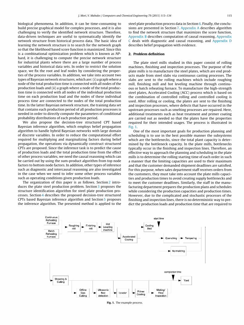
Chemi
bbcdnlsihfvsttnpttpttnp
BaorpCoobfsis
dscCt
J. Mori, V. Mahalec / Computers and
iological phenomena. In addition, it can be time-consuming touild precise graphical model for complex processes, and it is alsohallenging to verify the identified network structure. Therefore,ata-driven techniques are useful to systematically identify theetwork structure from historical process data. The basic idea of
earning the network structure is to search for the network grapho that the likelihood based score function is maximized. Since thiss a combinational optimization problem which is known as NP-ard, it is challenging to compute the precise network structure
or industrial plants where there are a large number of processariables and historical data sets. In order to restrict the solutionpace, we fix the root and leaf nodes by considering the proper-ies of the process variables. In addition, we take into account twoypes of Bayesian network structures, which are: (i) a graph where aode of the total production time is connected with all nodes of theroduction loads and (ii) a graph where a node of the total produc-ion time is connected with all nodes of the individual productionime on each production load and the nodes of these individualrocess time are connected to the nodes of the total productionime. In the latter Bayesian network structure, the training data sethat contains each production period of all production processes iseeded in order to directly compute the parameters of conditionalrobability distributions of each production period.
We also propose the decision-tree structured CPT basedayesian inference algorithm, which employs belief propagationlgorithm to handle hybrid Bayesian networks with large domainf discrete variables. In order to reduce the computational effortequired for multiplying and marginalizing factors during beliefropagation, the operations via dynamically construct structuredPTs are proposed. Since the inference task is to predict the causef production loads and the total production time from the effectf other process variables, we need the causal reasoning which cane carried out by using the sum-product algorithm from top nodeactors to bottom node factors. In addition, other types of inferenceuch as diagnostic and intercausal reasoning are also investigatedn the case when we need to infer some other process variablesuch as operating conditions given production loads.
The organization of this paper is as follows. Section 2 intro-uces the plate steel production problem. Section 3 proposes the
tructure identification algorithm for steel plate production pro-esses. Section 4 describes the proposed decision-tree structuredPTs based Bayesian inference algorithm and Section 5 proposeshe inference algorithm. The presented method is applied to theFig. 1. The examp
cal Engineering 79 (2015) 113–134 115
steel plate production process data in Section 6. Finally, the conclu-sions are presented in Section 7. Appendix A describes algorithmto find the network structure that maximizes the score function,Appendix B describes computation of causal reasoning, AppendixC deals with diagnostic and causal reasoning, and Appendix Ddescribes belief propagation with evidence.
2. Problem definition
The plate steel mills studied in this paper consist of rollingmachines, finishing and inspection processes. The purpose of theplate mills is to manufacture the steel plates, which are end prod-ucts made from steel slabs via continuous casting processes. Theslabs are sent to the rolling machines which include roughingmill, finishing mill and hot leveling machine through continu-ous or batch reheating furnace. To manufacture the high-strengthsteel plates, Accelerated Cooling (ACC) process which is based onthe combination of controlled rolling and controlled cooling isused. After rolling or cooling, the plates are sent to the finishingand inspection processes, where defects that have occurred in theupstream processes such as smelting processes are repaired. Here,additional treatments such as heat treatment and primer coatingare carried out as needed so that the plates have the propertiesrequired for their intended usages. The process is illustrated inFig. 1.
One of the most important goals for production planning andscheduling is to use in the best possible manner the subsystemswhich are the bottlenecks, since the total plant capacity is deter-mined by the bottleneck capacity. In the plate mills, bottleneckstypically occur in the finishing and inspection lines. Therefore, aneffective way to approach the planning and scheduling in the platemills is to determine the rolling starting time of each order in sucha manner that the limiting capacities are used to their maximumand that the customer demanded shipment deadlines are satisfied.For this purpose, when sales department staff receives orders fromthe customers, they must take into account the plate mills capaci-ties and production times to avoid creating supply bottlenecks andto meet the customer deadlines. Similarly, the staff in the manu-facturing department prepares the production plans and schedules
while considering the production capacities and production times.However, due to the complicated and stochastic processes of thefinishing and inspection lines, there is no deterministic way to pre-dict the production loads and production time that are required tole process.

1 Chemical Engineering 79 (2015) 113–134
dtlputPtttts
cd(io
i(abfl
1
2
Hsom
3p
iaptvdc
sseB
ootro
sme
Table 1System variables of steel production process.
Variable No. Variable description Domain size
1 Customer demand A 122 Customer demand B 23 Customer demand C 204 Customer demand D 205 Customer demand E 206 Customer demand F 10 (discretized)7 Customer demand G 10 (discretized)8 Customer demand H 10 (discretized)9 Customer demand I 10 (discretized)
10 Operating condition A 511 Operating condition B 212 Operating condition C 213 Operating condition D 214 Operating condition E 215 Operating condition F 216 Operating condition G 217 Production load A 218 Production load B 219 Production load C 220 Production load D 221 Production load E 222 Production load F 223 Production load G 224 Production load H 2
16 J. Mori, V. Mahalec / Computers and
etermine the production start times as required to avoid the bot-lenecks and meet the customer deadline. In this paper, productionoads represent the number of times that one plate or a set of totallates per day is processed at the corresponding production processnit. For instance, if 10 plates are processed at process A per day,hen the production load of process A is computed as 10 per day.roduction time for each plate or each customer order representshe time required to manufacture a product, starting from slabs tohe finished products. In this paper, since the processing time inhe inspection and finishing lines is a large part of the productionime, the production time represents the period from productiontart to completion as shown in Fig. 1.
When a steel plate manufacturer receives orders from austomer, the product demand is known while the operating con-itions, which are required to manufacture this specific productorder), are not available. On the other hand, at the manufactur-ng stage, all information about customer demands and detailedperating conditions is known.
Motivated by the above considerations, we can divide the tasksn plate steel production planning and scheduling into two parts:i) accurate prediction of the production loads and production timend (ii) optimization of the manufacturing plans and schedulesased on the production time prediction models. In this paper, weocus on the development of the prediction model for productionoads and production time. The prediction model needs to enable:
Estimation of the probability distributions of production loadsand production time, since the finishing and inspection linesinclude various sources of uncertainties and thus stochastic pre-diction models are desirable.
Dealing with unobservable (unavailable) variables, because it isdesirable to have a single model and avoid multiple models thatmeet with specific problems.
aving a single model with above properties enables planning andcheduling based on the same model which improves consistencyf decisions between planning and scheduling and also simplifiesodel maintenance.
. Identification of Bayesian networks structure for steellate production
In order to build a model which has the properties mentionedn the previous section, we develop the methods to compute prob-bility distributions of unknown states of production loads androduction times by using Bayesian network. Methodology to buildhe model will be illustrated by an example which has 21 discreteariables and 5 continuous variables as shown in Table 1. Each pro-uction load is assigned a binary variable having value of 1 if theorresponding production process is not needed, otherwise it is 2.
In this section, we propose the knowledge based date-driventructure learning algorithm to construct the Bayesian networktructure. In the subsequent sections, we will propose the param-ter estimation and inference approaches with the constructedayesian network structure.
The computational task for structure learning is to find theptimal graph such that the maximized Bayesian scores can bebtained, which is known as NP-hard problem. In order to reducehe computational effort, we allow some variables to be set at theoot nodes or the leaf nodes and also impose some constraints aboutrders of subsets of system variables.
First and the most important task for Bayesian inference is toynthesize the precise network structure. The most straightforwardethod is to design the network structure from process knowl-
dge. However, by-hand structure design requires in-depth process
25 Production load I 226 Process time Continuous
knowledge because identification of cause–effect relationships isneeded to characterize the complex physical, chemical and biolog-ical phenomena in systems. On the other hand, data-driven basedtechniques such as score function based structure learning are use-ful when there is lack of process knowledge or considered processesare too complicated to analyze.
The goal of structure learning is to find a network structure G thatis a good estimator for the data x. The most common approach isscore-based structure learning, which defines the structure learningproblem as an optimization problem (Koller and Friedman, 2009).A score function score(G : D) that measures how well the networkmodel fits the observed data D is defined. The computational task isto solve the combinational optimization problem of finding the net-work that has the highest score. The detailed algorithm to find thenetwork structure that maximizes the score function is explainedin Appendix A. It should be noted that this combinational optimiza-tion problem is known to be NP-hard (Chickering, 1996). Therefore,it is challenging to obtain the optimal graph for industrial plantswhich often include a large number of process variables.
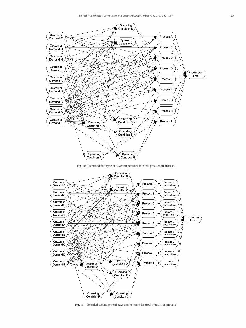
In order to reduce the computational cost, we incorporatethe fundamental process knowledge into the network structurelearning framework. As shown in the variable list of Table 1, allof our system variables belong to either customer demands oroperating conditions or production loads or production time. Onecan immediately notice that customer demands can be considered“cause variables” of all system variables in the Bayesian networkand are never impacted by either operating conditions, productionloads or production time. Therefore, the nodes of variables belong-ing to the customer demands should be placed on the root nodes inthe Bayesian network. Similarly, production loads are affected bythe customer demands, operating conditions or both and not viceversa. Taking into account above considerations, we propose twotypes of Bayesian networks as shown in Fig. 2. In both Bayesiannetworks, the nodes related to the customer demands are placedat the root nodes followed by operating conditions, productionloads and production time. The difference between two structures
is that in the second BN structure, the nodes associated with theproduction time at each production process are added betweenthe nodes of production loads and total production time while in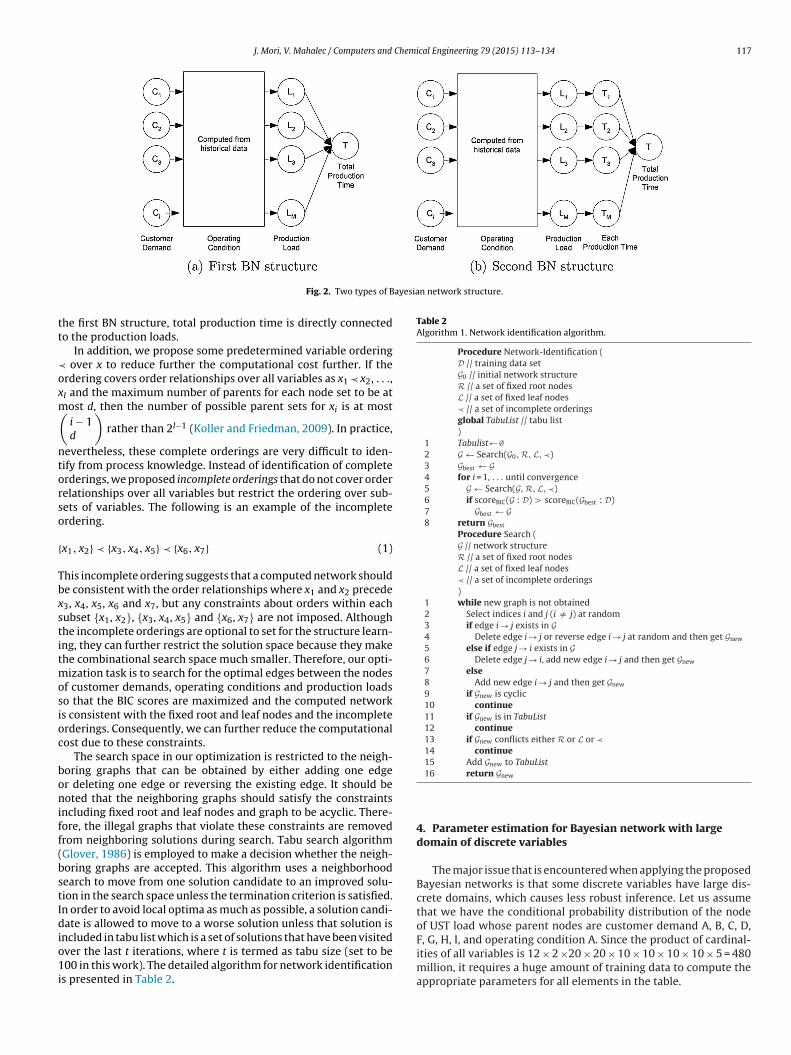
J. Mori, V. Mahalec / Computers and Chemical Engineering 79 (2015) 113–134 117
ayesian network structure.
tt
≺oxm(ntorso
{
Tbxstitmosioc
boniff(bstIdio1i
Table 2Algorithm 1. Network identification algorithm.
Procedure Network-Identification (D // training data setG0 // initial network structureR // a set of fixed root nodesL // a set of fixed leaf nodes≺ // a set of incomplete orderingsglobal TabuList // tabu list)
1 Tabulist← ∅2 G ← Search(G0, R, L, ≺)3 Gbest ← G4 for i = 1, . . . until convergence5 G ← Search(G, R, L, ≺)6 if scoreBIC(G : D) > scoreBIC(Gbest : D)7 Gbest ← G8 return Gbest
Procedure Search (G // network structureR // a set of fixed root nodesL // a set of fixed leaf nodes≺ // a set of incomplete orderings)
1 while new graph is not obtained2 Select indices i and j (i /= j) at random3 if edge i → j exists in G4 Delete edge i → j or reverse edge i → j at random and then get Gnew
5 else if edge j → i exists in G6 Delete edge j → i, add new edge i → j and then get Gnew
7 else8 Add new edge i → j and then get Gnew
9 if Gnew is cyclic10 continue11 if Gnew is in TabuList12 continue13 if Gnew conflicts either R or L or ≺14 continue15 Add Gnew to TabuList
Fig. 2. Two types of B
he first BN structure, total production time is directly connectedo the production loads.
In addition, we propose some predetermined variable ordering over x to reduce further the computational cost further. If therdering covers order relationships over all variables as x1 ≺ x2, . . .,I and the maximum number of parents for each node set to be atost d, then the number of possible parent sets for xi is at mosti − 1d
)rather than 2I−1 (Koller and Friedman, 2009). In practice,
evertheless, these complete orderings are very difficult to iden-ify from process knowledge. Instead of identification of completerderings, we proposed incomplete orderings that do not cover orderelationships over all variables but restrict the ordering over sub-ets of variables. The following is an example of the incompleterdering.
x1, x2} ≺ {x3, x4, x5} ≺ {x6, x7} (1)
his incomplete ordering suggests that a computed network shoulde consistent with the order relationships where x1 and x2 precede3, x4, x5, x6 and x7, but any constraints about orders within eachubset {x1, x2}, {x3, x4, x5} and {x6, x7} are not imposed. Althoughhe incomplete orderings are optional to set for the structure learn-ng, they can further restrict the solution space because they makehe combinational search space much smaller. Therefore, our opti-
ization task is to search for the optimal edges between the nodesf customer demands, operating conditions and production loadso that the BIC scores are maximized and the computed networks consistent with the fixed root and leaf nodes and the incompleterderings. Consequently, we can further reduce the computationalost due to these constraints.
The search space in our optimization is restricted to the neigh-oring graphs that can be obtained by either adding one edger deleting one edge or reversing the existing edge. It should beoted that the neighboring graphs should satisfy the constraints
ncluding fixed root and leaf nodes and graph to be acyclic. There-ore, the illegal graphs that violate these constraints are removedrom neighboring solutions during search. Tabu search algorithmGlover, 1986) is employed to make a decision whether the neigh-oring graphs are accepted. This algorithm uses a neighborhoodearch to move from one solution candidate to an improved solu-ion in the search space unless the termination criterion is satisfied.n order to avoid local optima as much as possible, a solution candi-ate is allowed to move to a worse solution unless that solution is
ncluded in tabu list which is a set of solutions that have been visitedver the last t iterations, where t is termed as tabu size (set to be00 in this work). The detailed algorithm for network identification
s presented in Table 2.
16 return Gnew
4. Parameter estimation for Bayesian network with largedomain of discrete variables
The major issue that is encountered when applying the proposedBayesian networks is that some discrete variables have large dis-crete domains, which causes less robust inference. Let us assumethat we have the conditional probability distribution of the nodeof UST load whose parent nodes are customer demand A, B, C, D,F, G, H, I, and operating condition A. Since the product of cardinal-
ities of all variables is 12 × 2 ×20 × 20 × 10 × 10 × 10 × 10 × 5 = 480million, it requires a huge amount of training data to compute theappropriate parameters for all elements in the table.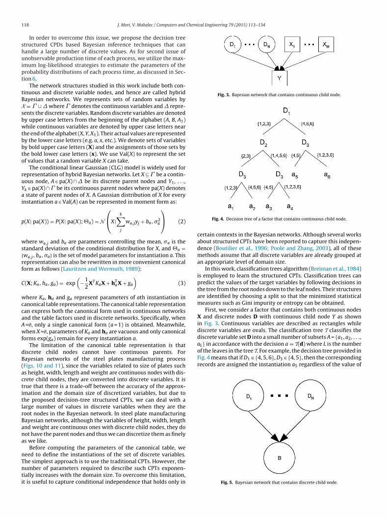
1 Chemical Engineering 79 (2015) 113–134
shuipt
tBXsbwtbbto
ruYai
p
ws{rf
C
wccaAwf
dB(actitlrBana
nTnti
Fig. 3. Bayesian network that contains continuous child node.
L
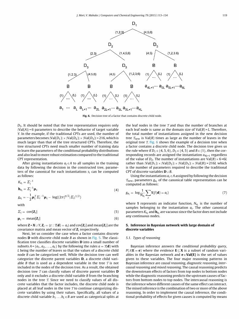
of the leaves in the tree T. For example, the decision tree provided inFig. 4 means that if D1 ∈ {4, 5, 6}, D3 ∈ {4, 5}, then the correspondingrecords are assigned the instantiation a5 regardless of the value of
18 J. Mori, V. Mahalec / Computers and
In order to overcome this issue, we propose the decision treetructured CPDs based Bayesian inference techniques that canandle a large number of discrete values. As for second issue ofnobservable production time of each process, we utilize the max-
mum log-likelihood strategies to estimate the parameters of therobability distributions of each process time, as discussed in Sec-ion 6.
The network structures studied in this work include both con-inuous and discrete variable nodes, and hence are called hybridayesian networks. We represents sets of random variables by
= � ∪ � where � denotes the continuous variables and � repre-ents the discrete variables. Random discrete variables are denotedy upper case letters from the beginning of the alphabet (A, B, A1)hile continuous variables are denoted by upper case letters near
he end of the alphabet (X, Y, X1). Their actual values are representedy the lower case letters (e.g. a, x, etc.). We denote sets of variablesy bold upper case letters (X) and the assignments of those sets byhe bold lower case letters (x). We use Val(X) to represent the setf values that a random variable X can take.
The conditional linear Gaussian (CLG) model is widely used forepresentation of hybrid Bayesian networks. Let X ⊆ � be a contin-ous node, A ∈ pa(X) ∩ � be its discrete parent nodes and Y1, . . .,k ∈ pa(X) ∩ � be its continuous parent nodes where pa(X) denotes
state of parent nodes of X. A Gaussian distribution of X for everynstantiation a ∈ Val(A) can be represented in moment form as:
(X| pa(X)) = P(X| pa(X); �a) = N
⎛⎝X| k∑
j
wa,jyj + ba, �2a
⎞⎠ (2)
here wa,j and ba are parameters controlling the mean, �a is thetandard deviation of the conditional distribution for X, and �a =wa,j, ba, �a} is the set of model parameters for instantiation a. Thisepresentation can also be rewritten in more convenient canonicalorm as follows (Lauritzen and Wermuth, 1989):
(X; Ka, ha, ga) = exp(−1
2XTKaX + hTaX + ga
)(3)
here Ka, ha and ga represent parameters of ath instantiation inanonical table representations. The canonical table representationan express both the canonical form used in continuous networksnd the table factors used in discrete networks. Specifically, when
=∅, only a single canonical form (a = 1) is obtained. Meanwhile,hen X =∅, parameters of Ka and ha are vacuous and only canonical
orms exp(ga) remain for every instantiation a.The limitation of the canonical table representation is that
iscrete child nodes cannot have continuous parents. Forayesian networks of the steel plates manufacturing processFigs. 10 and 11), since the variables related to size of plates suchs height, width, length and weight are continuous nodes with dis-rete child nodes, they are converted into discrete variables. It isrue that there is a trade-off between the accuracy of the approx-mation and the domain size of discretized variables, but due tohe proposed decision-tree structured CPTs, we can deal with aarge number of values in discrete variables when they are theoot nodes in the Bayesian network. In steel plate manufacturingayesian networks, although the variables of height, width, lengthnd weight are continuous ones with discrete child nodes, they doot have the parent nodes and thus we can discretize them as finelys we like.
Before computing the parameters of the canonical table, weeed to define the instantiations of the set of discrete variables.
he simplest approach is to use the traditional CPTs. However, theumber of parameters required to describe such CPTs exponen-ially increases with the domain size. To overcome this limitation,t is useful to capture conditional independence that holds only inFig. 4. Decision tree of a factor that contains continuous child node.
certain contexts in the Bayesian networks. Although several worksabout structured CPTs have been reported to capture this indepen-dence (Boutilier et al., 1996; Poole and Zhang, 2003), all of thesemethods assume that all discrete variables are already grouped atan appropriate level of domain size.
In this work, classification trees algorithm (Breiman et al., 1984)is employed to learn the structured CPTs. Classification trees canpredict the values of the target variables by following decisions inthe tree from the root nodes down to the leaf nodes. Their structuresare identified by choosing a split so that the minimized statisticalmeasures such as Gini impurity or entropy can be obtained.
First, we consider a factor that contains both continuous nodesX and discrete nodes D with continuous child node Y as shownin Fig. 3. Continuous variables are described as rectangles whilediscrete variables are ovals. The classification tree T classifies thediscrete variable set D into a small number of subsets A = {a1, a2, . . .,a } in accordance with the decision a = T(d) where L is the number
Fig. 5. Bayesian network that contains discrete child node.
J. Mori, V. Mahalec / Computers and Chemical Engineering 79 (2015) 113–134 119
r that
D|YpmttaC
dta
w
˙
�
wc
nfisLncaidoncpcd
Fig. 6. Decision tree of a facto
3. It should be noted that the tree representation requires onlyVal(A)| = 6 parameters to describe the behavior of target variable. In the example, if the traditional CPTs are used, the number ofarameters becomes |Val(D1)| × |Val(D2)| × |Val(D3)| = 216, which isuch larger than that of the tree structured CPTs. Therefore, the
ree structured CPTs need much smaller number of training datao learn the parameters of the conditional probability distributionsnd also lead to more robust estimation compared to the traditionalPT representation.
After giving instantiations ai ∈ A to all samples in the trainingata by following the decision in the constructed tree, parame-ers of the canonical for each instantiations si can be computeds follows:
Kai = ˙−1i
hai = ˙−1i
�i
gai = −12
�Ti ˙i
−1�i − log((2�)n/2|˙i|1/2)
(4)
ith
i = cov[Zi] (5)
i = mean[Zi] (6)
here Z = X ∪ Y, Zi = {z : T(d) = ai} and cov[Zi] and mean[Zi] are theovariance matrix and mean vector of Zi respectively.
Next, let us consider the case when a factor contains discreteodes D with discrete child node B as shown in Fig. 5. The classi-cation tree classifies discrete variables D into a small number ofubsets A = {a1, a2, . . ., aL} by the following the rules a = T(d) with
being the number of leaves so that the values of a discrete childode B can be categorized well. While the decision tree can wellategorize the discrete parent variables D, a discrete child vari-ble B that is used as a dependent variable in the tree T is notncluded in the nodes of the decision tree. As a result, the obtainedecision tree T can classify values of discrete parent variables Dnly and it excludes a discrete child variable B from the branchingodes in the tree T. Since we need to classify values of all dis-
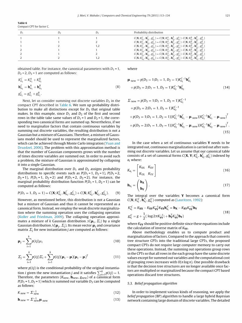
rete variables that the factor includes, the discrete child node islaced at all leaf nodes in the tree T to continue categorizing dis-rete variables by using their values. Specifically, all values of aiscrete child variable b1 . . . bL ∈ B are used as categorical splits atcontains discrete child node.
the leaf nodes in the tree T and thus the number of branches ateach leaf node is same as the domain size of Val(B) = L. Therefore,the total number of instantiations assigned in the new decisiontree Tnew is Val(B) times as large as the number of leaves in theoriginal tree T. Fig. 6 shows the example of a decision tree whena factor contains a discrete child node. The decision tree gives usthe rule where if D1 ∈ {4, 5, 6}, D3 ∈ {4, 5} and B ∈ {1}, then the cor-responding records are assigned the instantiation a4L+1 regardlessof the value of D2. The number of instantiations are Val(B) × 6 =6Lrather than |Val(D1)| × |Val(D2)| × |Val(D3)| × |Val(B)| = 216L whichis the number of parameters required to describe the traditionalCPT of discrete variables D ∪ B.
Using the instantiations ai ∈ A assigned by following the decisionTnew, parameters gai of the canonical table representation can becomputed as follows:
gai = log1Nai
∑z
1(f (d) = ai) (7)
where 1 represents an indicator function, Nai is the number ofsamples belonging to the instantiation ai. The other canonicalparameters Kai and hai are vacuous since the factor does not includeany continuous nodes.
5. Inference in Bayesian network with large domain ofdiscrete variables
5.1. Types of reasoning
Bayesian inference answers the conditional probability query,P(X|E = e) where the evidence E ⊆ X is a subset of random vari-ables in the Bayesian network and e ∈ Val(E) is the set of valuesgiven to these variables. The four major reasoning patterns inBayesian inference are causal reasoning, diagnostic reasoning, inter-causal reasoning and mixed reasoning. The causal reasoning predictsthe downstream effects of factors from top nodes to bottom nodeswhile the diagnostic reasoning predicts the upstream causes of fac-tors from bottom nodes to top nodes. The intercausal reasoning is
the inference where different causes of the same effect can interact.The mixed inference is the combination of two or more of the abovereasoning. In order to implement the causal inference, the condi-tional probability of effects for given causes is computed by means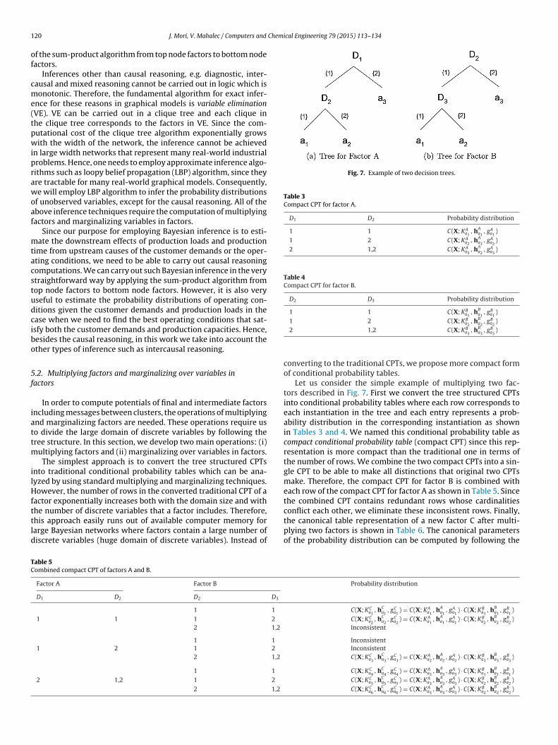
1 Chemical Engineering 79 (2015) 113–134
of
cme(tpwiprawoaf
mtacstudcibo
5f
iattm
ilHfttld
Fig. 7. Example of two decision trees.
Table 3Compact CPT for factor A.
D1 D2 Probability distribution
1 1 C(X; KAa1, hAa1
, gAa1)
1 2 C(X; KAa2, hAa3
, gAa2)
2 1,2 C(X; KAa3, hAa2
, gAa3)
Table 4Compact CPT for factor B.
D2 D3 Probability distribution
1 1 C(X; KBa1, hBa1
, gBa1)
1 2 C(X; KB , hB , gB )
TC
20 J. Mori, V. Mahalec / Computers and
f the sum-product algorithm from top node factors to bottom nodeactors.
Inferences other than causal reasoning, e.g. diagnostic, inter-ausal and mixed reasoning cannot be carried out in logic which isonotonic. Therefore, the fundamental algorithm for exact infer-
nce for these reasons in graphical models is variable eliminationVE). VE can be carried out in a clique tree and each clique inhe clique tree corresponds to the factors in VE. Since the com-utational cost of the clique tree algorithm exponentially growsith the width of the network, the inference cannot be achieved
n large width networks that represent many real-world industrialroblems. Hence, one needs to employ approximate inference algo-ithms such as loopy belief propagation (LBP) algorithm, since theyre tractable for many real-world graphical models. Consequently,e will employ LBP algorithm to infer the probability distributions
f unobserved variables, except for the causal reasoning. All of thebove inference techniques require the computation of multiplyingactors and marginalizing variables in factors.
Since our purpose for employing Bayesian inference is to esti-ate the downstream effects of production loads and production
ime from upstream causes of the customer demands or the oper-ting conditions, we need to be able to carry out causal reasoningomputations. We can carry out such Bayesian inference in the verytraightforward way by applying the sum-product algorithm fromop node factors to bottom node factors. However, it is also veryseful to estimate the probability distributions of operating con-itions given the customer demands and production loads in thease when we need to find the best operating conditions that sat-sfy both the customer demands and production capacities. Hence,esides the causal reasoning, in this work we take into account thether types of inference such as intercausal reasoning.
.2. Multiplying factors and marginalizing over variables inactors
In order to compute potentials of final and intermediate factorsncluding messages between clusters, the operations of multiplyingnd marginalizing factors are needed. These operations require uso divide the large domain of discrete variables by following theree structure. In this section, we develop two main operations: (i)
ultiplying factors and (ii) marginalizing over variables in factors.The simplest approach is to convert the tree structured CPTs
nto traditional conditional probability tables which can be ana-yzed by using standard multiplying and marginalizing techniques.owever, the number of rows in the converted traditional CPT of a
actor exponentially increases both with the domain size and with
he number of discrete variables that a factor includes. Therefore,his approach easily runs out of available computer memory forarge Bayesian networks where factors contain a large number ofiscrete variables (huge domain of discrete variables). Instead ofable 5ombined compact CPT of factors A and B.
Factor A Factor B
D1 D2 D2 D3
1 1
1 1 1 2
2 1,2
1 1
1 2 1 2
2 1,2
1 1
2 1,2 1 2
2 1,2
a2 a2 a2
2 1,2 C(X; KBa3, hBa3
, gBa3)
converting to the traditional CPTs, we propose more compact formof conditional probability tables.
Let us consider the simple example of multiplying two fac-tors described in Fig. 7. First we convert the tree structured CPTsinto conditional probability tables where each row corresponds toeach instantiation in the tree and each entry represents a prob-ability distribution in the corresponding instantiation as shownin Tables 3 and 4. We named this conditional probability table ascompact conditional probability table (compact CPT) since this rep-resentation is more compact than the traditional one in terms ofthe number of rows. We combine the two compact CPTs into a sin-gle CPT to be able to make all distinctions that original two CPTsmake. Therefore, the compact CPT for factor B is combined witheach row of the compact CPT for factor A as shown in Table 5. Sincethe combined CPT contains redundant rows whose cardinalitiesconflict each other, we eliminate these inconsistent rows. Finally,the canonical table representation of a new factor C after multi-
plying two factors is shown in Table 6. The canonical parametersof the probability distribution can be computed by following theProbability distribution
C(X; KCa1, hCa1
, gCa1) = C(X; KAa1
, hAa1, gAa1
) · C(X; KBa1, hBa1
, gBa1)
C(X; KCa2, hCa2
, gCa2) = C(X; KAa1
, hAa1, gAa1
) · C(X; KBa2, hBa2
, gBa2)
Inconsistent
InconsistentInconsistentC(X; KCa3
, hCa3, gCa3
) = C(X; KAa2, hAa2
, gAa2) · C(X; KBa3
, hBa3, gBa3
)
C(X; KCa4, hCa4
, gCa4) = C(X; KAa3
, hAa3, gAa3
) · C(X; KBa1, hBa1
, gBa1)
C(X; KCa5, hCa5
, gCa5) = C(X; KAa3
, hAa3, gAa3
) · C(X; KBa2, hBa2
, gBa2)
C(X; KCa6, hCa6
, gCa6) = C(X; KAa3
, hAa3, gAa3
) · C(X; KBa2, hBa2
, gBa2)
J. Mori, V. Mahalec / Computers and Chemical Engineering 79 (2015) 113–134 121
Table 6Compact CPT for factor C.
D1 D2 D3 Probability distribution
1 1 1 C(X; KCa1, hCa1
, gCa1) = C(X; KAa1
, hAa1, gAa1
) · C(X; KBa1, hBa1
, gBa1)
1 1 2 C(X; KCa2, hCa2
, gCa2) = C(X; KAa1
, hAa1, gAa1
) · C(X; KBa2, hBa2
, gBa2)
1 2 1,2 C(X; KCa3, hCa3
, gCa3) = C(X; KAa2
, hAa2, gAa2
) · C(X; KBa3, hBa3
, gBa3)
2 1 1 C(X; KC , hC , gC ) = C(X; KA , hA , gA ) · C(X; KB , hB , gB )
oD
cbmrsnsGiwDtoai
dDmc
P
Hbct(mGm
�
˙
wtTPa
K
h
2 1 2
2 2 1,2
btained table. For instance, the canonical parameters with D1 = 1,2 = 2, D3 = 1 are computed as follows:
KCa1= KAa1
+ KBa1
hCa1= hAa1
+ hBa1
gCa1= gAa1
+ gBa1.
(8)
Next, let us consider summing out discrete variables D3 in theompact CPT described in Table 6. We sum up probability distri-ution to make all distinctions except for D3 that original tableakes. In this example, since D1 and D2 of the first and second
ows in the table take same values of D1 = 1 and D2 = 1, the corre-ponding two canonical forms are summed up. Nevertheless, if weeed to marginalize factors that contain continuous variables byumming out discrete variables, the resulting distribution is not aaussian but a mixture of Gaussians. Therefore, a mixture of Gauss-
ans model should be used to represent the marginalized factors,hich can be achieved through Monte Carlo integration (Yuan andruzdzel, 2006). The problem with this approximation method is
hat the number of Gaussian components grows with the numberf times discrete variables are summed out. In order to avoid such
problem, the mixture of Gaussian is approximated by collapsingt into a single Gaussian.
The marginal distribution over D1 and D2 assigns probabilityistributions to specific events such as P(D1 = 1, D2 = 1), P(D1 = 2,2 = 1), P(D1 = 1, D2 = 2) and P(D1 = 2, D2 = 2). For instance, thearginal probability distribution function P(D1 = 1, D2 = 1) can be
omputed as follows:
(D1 = 1, D2 = 1) = C(X; KCa1, hCa1
, gCa1) + C(X; KCa2
, hCa2, gCa2
). (9)
owever, as mentioned before, this distribution is not a Gaussianut a mixture of Gaussian and thus it cannot be represented as aanonical form. Instead, we employ the weak discrete marginaliza-ion where the summing operation uses the collapsing operationKoller and Friedman, 2009). The collapsing operation approxi-
ates a mixture of k Gaussian distribution N(�i, ˙i) by a singleaussian distribution N(�j, ˙j). Its mean vector �j and covarianceatrix ˙j for new instantiation j are computed as follows:
j =k∑i=1
p(i|j)�i (10)
j =k∑i=1
p(i|j)˙i +k∑i=1
p(i|j)(�i − �)(�i − �)T (11)
here p(i|j) is the conditional probability of the original instantia-ion i given the new instantiation j and it satisfies
∑ki=1p(i|j) = 1.
herefore, the parameters (Knew, hnew, gnew) of a canonical form(D1 = 1, D2 = 1) which is summed out variable D3 can be computed
s follows:new = ˙−1new (12)
new = ˙−1new� new (13)
a4 a4 a4 a3 a3 a3 a1 a1 a1
C(X; KCa5, hCa5
, gCa5) = C(X; KAa3
, hAa3, gAa3
) · C(X; KBa2, hBa2
, gBa2)
C(X; KCa6, hCa6
, gCa6) = C(X; KAa3
, hAa3, gAa3
) · C(X; KBa2, hBa2
, gBa2)
where
� new = p(D3 = 1|D1 = 1, D2 = 1)KC−1a1
hCa1
+ p(D3 = 2|D1 = 1, D2 = 1)KC−1a2
hCa2(14)
˙ new = p(D3 = 1|D1 = 1, D2 = 1)KC−1a1
+ p(D3 = 2|D1 = 1, D2 = 1)KC−1a2
+ p(D3 = 1|D1 = 1, D2 = 1)(KC−1a1
hCa1− � new)(KC−1
a1hCa1− � new)
T
+ p(D3 = 2|D1 = 1, D2 = 1)(KC−1a2
hCa2− � new)(KC−1
a2hCa2− � new)
T.
(15)
In the case when a set of continuous variables Y needs to beintegrated out, continuous marginalization is carried out after sum-ming out discrete variables. Let us assume that our canonical tableconsists of a set of canonical forms C(X, Y; KCai , hCai , gCai ) indexed byai where:
Kai =[KXX KXY
KYX KYY
](16)
hai =(
hX
hY
). (17)
The integral over the variables Y becomes a canonical formC(X; K ′Cai , h′Cai , g′Cai ) computed as (Lauritzen, 1992):
K ′Cai = KXX − KXYK−1YY KYXh′Cai = hX − KXYK
−1YY hY
g′Cai = g + 12
( log|2�K−1YY | + hTYK
−1YY hY)
(18)
where KYY should be positive definite since these equations includethe calculation of inverse matrix of KYY.
Above methodology enables us to compute product andmarginalization of factors. Compared to the approach that convertstree structure CPTs into the traditional large CPTs, the proposedcompact CPTs do not require large computer memory to carry outthese operations. Instead, the summing out operations group rowsin the CPTs so that all rows in the each group have the same discretevalues except for summed out variables and the computational costof grouping rows increases with O(n log n). One possible drawbackis that the decision tree structures are no longer available once fac-tors are multiplied or marginalized because the compact CPT basedoperations discard tree structures.
5.3. Belief propagation algorithm
In order to implement various kinds of reasoning, we apply thebelief propagation (BP) algorithm to handle a large hybrid Bayesiannetwork containing large domain of discrete variables. The detailed
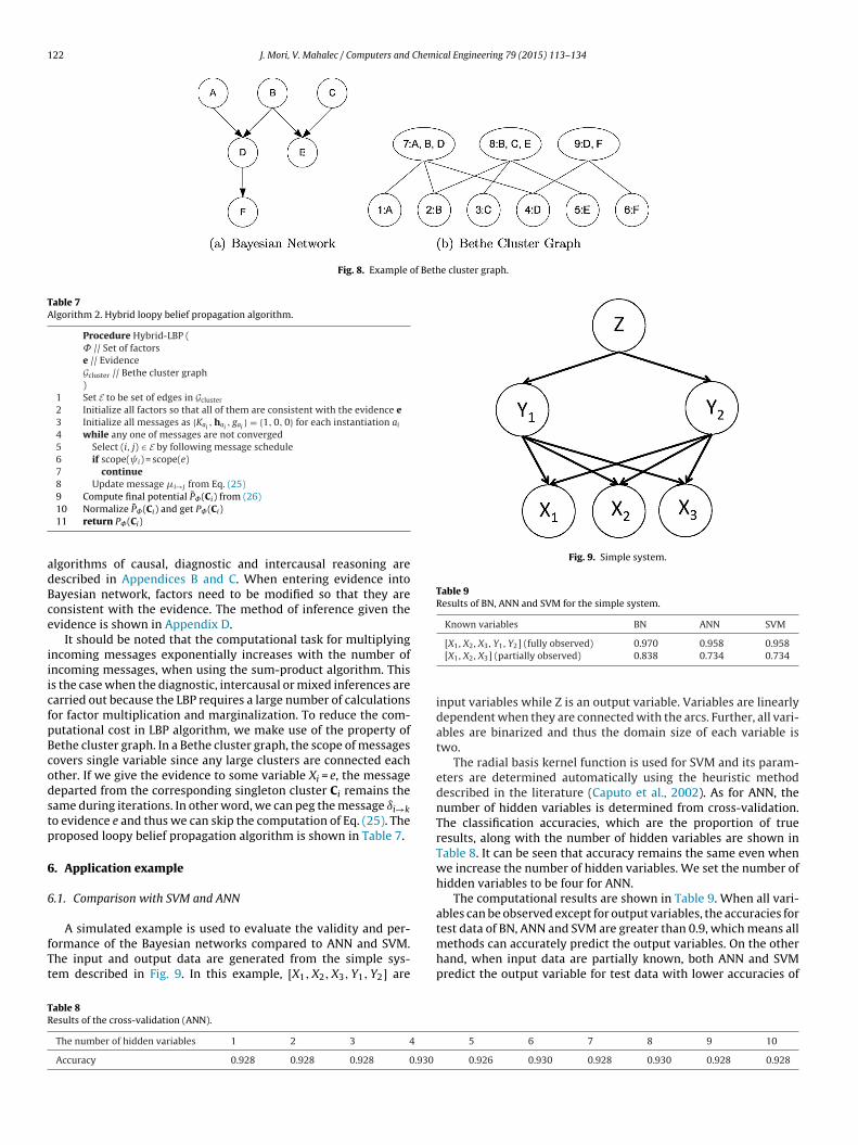
122 J. Mori, V. Mahalec / Computers and Chemical Engineering 79 (2015) 113–134
Fig. 8. Example of Bethe cluster graph.
Table 7Algorithm 2. Hybrid loopy belief propagation algorithm.
Procedure Hybrid-LBP (˚ // Set of factorse // EvidenceGcluster // Bethe cluster graph)
1 Set E to be set of edges in Gcluster
2 Initialize all factors so that all of them are consistent with the evidence e3 Initialize all messages as {Kai , hai , gai } = {1, 0, 0} for each instantiation ai
4 while any one of messages are not converged5 Select (i, j) ∈ E by following message schedule6 if scope( i) = scope(e)7 continue8 Update message �i→j from Eq. (25)9 Compute final potential P̃˚(Ci) from (26)
adBce
iiicfpBcodstp
6
6
fTt
Fig. 9. Simple system.
Table 9Results of BN, ANN and SVM for the simple system.
Known variables BN ANN SVM
TR
10 Normalize P̃˚(Ci) and get P˚(Ci)11 return P˚(Ci)
lgorithms of causal, diagnostic and intercausal reasoning areescribed in Appendices B and C. When entering evidence intoayesian network, factors need to be modified so that they areonsistent with the evidence. The method of inference given thevidence is shown in Appendix D.
It should be noted that the computational task for multiplyingncoming messages exponentially increases with the number ofncoming messages, when using the sum-product algorithm. Thiss the case when the diagnostic, intercausal or mixed inferences arearried out because the LBP requires a large number of calculationsor factor multiplication and marginalization. To reduce the com-utational cost in LBP algorithm, we make use of the property ofethe cluster graph. In a Bethe cluster graph, the scope of messagesovers single variable since any large clusters are connected eachther. If we give the evidence to some variable Xi = e, the messageeparted from the corresponding singleton cluster Ci remains theame during iterations. In other word, we can peg the message ıi→ko evidence e and thus we can skip the computation of Eq. (25). Theroposed loopy belief propagation algorithm is shown in Table 7.
. Application example
.1. Comparison with SVM and ANN
A simulated example is used to evaluate the validity and per-ormance of the Bayesian networks compared to ANN and SVM.he input and output data are generated from the simple sys-em described in Fig. 9. In this example, [X1, X2, X3, Y1, Y2] are
able 8esults of the cross-validation (ANN).
The number of hidden variables 1 2 3 4
Accuracy 0.928 0.928 0.928 0.930
[X1, X2, X3, Y1, Y2] (fully observed) 0.970 0.958 0.958[X1, X2, X3] (partially observed) 0.838 0.734 0.734
input variables while Z is an output variable. Variables are linearlydependent when they are connected with the arcs. Further, all vari-ables are binarized and thus the domain size of each variable istwo.
The radial basis kernel function is used for SVM and its param-eters are determined automatically using the heuristic methoddescribed in the literature (Caputo et al., 2002). As for ANN, thenumber of hidden variables is determined from cross-validation.The classification accuracies, which are the proportion of trueresults, along with the number of hidden variables are shown inTable 8. It can be seen that accuracy remains the same even whenwe increase the number of hidden variables. We set the number ofhidden variables to be four for ANN.
The computational results are shown in Table 9. When all vari-ables can be observed except for output variables, the accuracies fortest data of BN, ANN and SVM are greater than 0.9, which means all
methods can accurately predict the output variables. On the otherhand, when input data are partially known, both ANN and SVMpredict the output variable for test data with lower accuracies of5 6 7 8 9 10
0.926 0.930 0.928 0.930 0.928 0.928
J. Mori, V. Mahalec / Computers and Chemical Engineering 79 (2015) 113–134 123
Fig. 10. Identified first type of Bayesian network for steel production process.
Fig. 11. Identified second type of Bayesian network for steel production process.
124 J. Mori, V. Mahalec / Computers and Chemical Engineering 79 (2015) 113–134
0 0.5 10
0.2
0.4
0.6
0.8
1correlation=0.681RMSE=0.076
Process A
Predicted probability
Act
ual p
roba
bilit
y
0 0.5 10
0.2
0.4
0.6
0.8
1correlation=0.892RMSE=0.107
Process B
Predicted probability
Act
ual p
roba
bilit
y
0 0.5 10
0.2
0.4
0.6
0.8
1correlation=0.93RMSE=0.049
Process C
Predicted probability
Act
ual p
roba
bilit
y
0 0.5 10
0.2
0.4
0.6
0.8
1correlation=0.889RMSE=0.097
Process D
Predicted probability
Act
ual p
roba
bilit
y
0 0.5 10
0.2
0.4
0.6
0.8
1correlation=0.914RMSE=0.185
Process E
Predicted probability
Act
ual p
roba
bilit
y
0 0.5 10
0.2
0.4
0.6
0.8
1correlation=0.957RMSE=0.123
Process F
Predicted probability
Act
ual p
roba
bilit
y
0 0.5 10
0.2
0.4
0.6
0.8
1correlation=0.981RMSE=0.028
Process G
Act
ual p
roba
bilit
y
0 0.5 10
0.2
0.4
0.6
0.8
1correlation=0.164RMSE=0.098
Process H
icted
Act
ual p
roba
bilit
y
0 0.5 10
0.2
0.4
0.6
0.8
1correlation=0.031RMSE=0.097
Process I
Act
ual p
roba
bilit
y
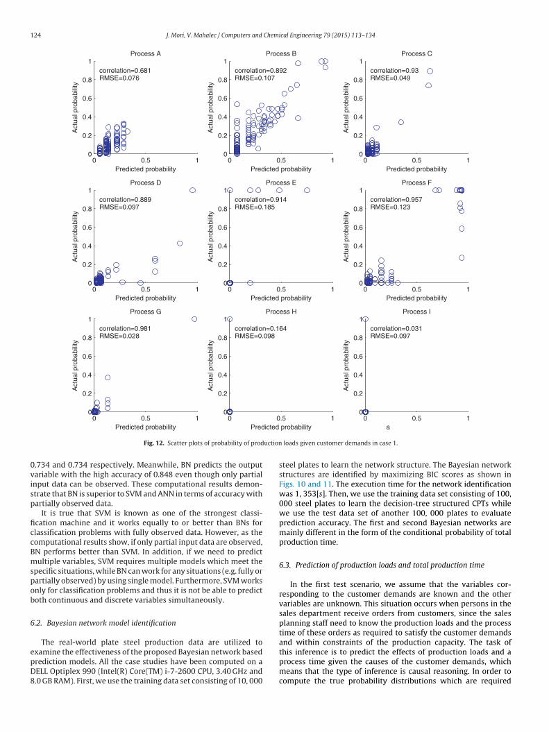
uction
0visp
ficcBmspob
6
epD8
Predicted probability Pred
Fig. 12. Scatter plots of probability of prod
.734 and 0.734 respectively. Meanwhile, BN predicts the outputariable with the high accuracy of 0.848 even though only partialnput data can be observed. These computational results demon-trate that BN is superior to SVM and ANN in terms of accuracy withartially observed data.
It is true that SVM is known as one of the strongest classi-cation machine and it works equally to or better than BNs forlassification problems with fully observed data. However, as theomputational results show, if only partial input data are observed,N performs better than SVM. In addition, if we need to predictultiple variables, SVM requires multiple models which meet the
pecific situations, while BN can work for any situations (e.g. fully orartially observed) by using single model. Furthermore, SVM worksnly for classification problems and thus it is not be able to predictoth continuous and discrete variables simultaneously.
.2. Bayesian network model identification
The real-world plate steel production data are utilized to
xamine the effectiveness of the proposed Bayesian network basedrediction models. All the case studies have been computed on aELL Optiplex 990 (Intel(R) Core(TM) i-7-2600 CPU, 3.40 GHz and.0 GB RAM). First, we use the training data set consisting of 10, 000probability a
loads given customer demands in case 1.
steel plates to learn the network structure. The Bayesian networkstructures are identified by maximizing BIC scores as shown inFigs. 10 and 11. The execution time for the network identificationwas 1, 353[s]. Then, we use the training data set consisting of 100,000 steel plates to learn the decision-tree structured CPTs whilewe use the test data set of another 100, 000 plates to evaluateprediction accuracy. The first and second Bayesian networks aremainly different in the form of the conditional probability of totalproduction time.
6.3. Prediction of production loads and total production time
In the first test scenario, we assume that the variables cor-responding to the customer demands are known and the othervariables are unknown. This situation occurs when persons in thesales department receive orders from customers, since the salesplanning staff need to know the production loads and the processtime of these orders as required to satisfy the customer demandsand within constraints of the production capacity. The task of
this inference is to predict the effects of production loads and aprocess time given the causes of the customer demands, whichmeans that the type of inference is causal reasoning. In order tocompute the true probability distributions which are required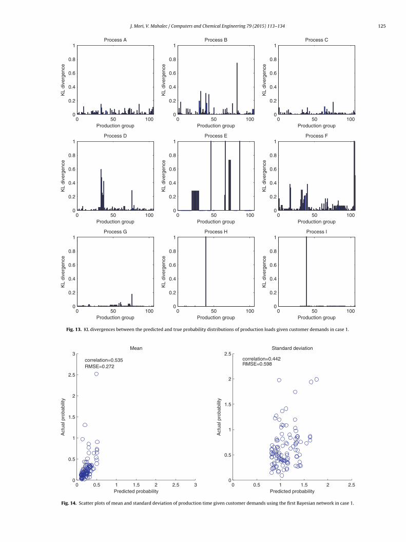
J. Mori, V. Mahalec / Computers and Chemical Engineering 79 (2015) 113–134 125
0 50 1000
0.2
0.4
0.6
0.8
1Process A
Production group
KL
dive
rgen
ce
0 50 1000
0.2
0.4
0.6
0.8
1Process B
Production group
KL
dive
rgen
ce
0 50 1000
0.2
0.4
0.6
0.8
1Process C
Production group
KL
dive
rgen
ce
0 50 1000
0.2
0.4
0.6
0.8
1Process D
Production group
KL
dive
rgen
ce
0 50 1000
0.2
0.4
0.6
0.8
1Process E
Production group
KL
dive
rgen
ce
0 50 1000
0.2
0.4
0.6
0.8
1Process F
Production group
KL
dive
rgen
ce
0 50 1000
0.2
0.4
0.6
0.8
1Process G
Production group
KL
dive
rgen
ce
0 50 1000
0.2
0.4
0.6
0.8
1Process H
Production group
KL
dive
rgen
ce
0 50 1000
0.2
0.4
0.6
0.8
1Process I
Production group
KL
dive
rgen
ce
Fig. 13. KL divergences between the predicted and true probability distributions of production loads given customer demands in case 1.
0 0.5 1 1.5 2 2.5 30
0.5
1
1.5
2
2.5
3correlation=0.535RMSE=0.272
Mean
Predicted probability
Act
ual p
roba
bilit
y
0 0.5 1 1.5 2 2.50
0.5
1
1.5
2
2.5correlation=0.442RMSE=0.598
Standard deviation
Predicted probability
Act
ual p
roba
bilit
y
Fig. 14. Scatter plots of mean and standard deviation of production time given customer demands using the first Bayesian network in case 1.
126 J. Mori, V. Mahalec / Computers and Chemical Engineering 79 (2015) 113–134
0 10 20 30 40 50 60 70 80 90 1000
0.5
1
1.5
2
2.5
3
3.5
4
4.5
5
Production group
KL
dive
rgen
ce
Fig. 15. KL divergences between the predicted and true probability distributions of production time given customer demands using the first Bayesian network in case 1.
0 0. 5 1 1. 5 2 2. 5 30
0.5
1
1.5
2
2.5
3correlation=0.696RMSE=0.23 2
Mean
Predicted probability
Act
ual p
roba
bilit
y
0 0. 5 1 1. 5 2 2. 50
0.5
1
1.5
2
2.5correlation=0.587RMSE=0.474
Standard deviation
Predicted probability
Act
ual p
roba
bilit
y
Fig. 16. Scatter plots of mean and standard deviation of production time given customer demands using the second Bayesian network in case 1.
0 10 20 30 40 50 60 70 80 90 1000
0.5
1
1.5
2
2.5
3
3.5
4
4.5
5
Production group
KL
dive
rgen
ce
Fig. 17. KL divergences between the predicted and true probability distributions of production time given customer demands using the second Bayesian network in case 1.
J. Mori, V. Mahalec / Computers and Chemical Engineering 79 (2015) 113–134 127
0 0.5 10
0.2
0.4
0.6
0.8
1correlation=0.681RMSE=0.076
Process A
Predicted probability
Act
ual p
roba
bilit
y
0 0.5 10
0.2
0.4
0.6
0.8
1correlation=0.892RMSE=0.107
Process B
Predicted probability
Act
ual p
roba
bilit
y
0 0.5 10
0.2
0.4
0.6
0.8
1correlation=0.931RMSE=0.049
Process C
Predicted probability
Act
ual p
roba
bilit
y
0 0.5 10
0.2
0.4
0.6
0.8
1correlation=0.978RMSE=0.041
Process D
Predicted probability
Act
ual p
roba
bilit
y
0 0.5 10
0.2
0.4
0.6
0.8
1correlation=1RMSE=0.001
Process E
Predicted probability
Act
ual p
roba
bilit
y
0 0.5 10
0.2
0.4
0.6
0.8
1correlation=0.99RMSE=0.06
Process F
Predicted probability
Act
ual p
roba
bilit
y
0 0.5 10
0.2
0.4
0.6
0.8
1correlation=0.982RMSE=0.028
Process G
Act
ual p
roba
bilit
y
0 0.5 10
0.2
0.4
0.6
0.8
1correlation=1RMSE=0.001
Process H
icted
Act
ual p
roba
bilit
y
0 0.5 10
0.2
0.4
0.6
0.8
1correlation=1RMSE=0.023
Process I
Act
ual p
roba
bilit
y
given
fpcppcbtp
tFaKbstoawdad
Predicted probability Pred
Fig. 18. Scatter plots of probability of production loads
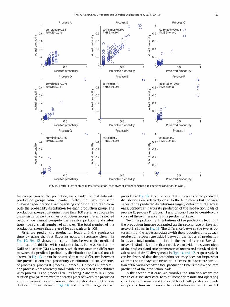
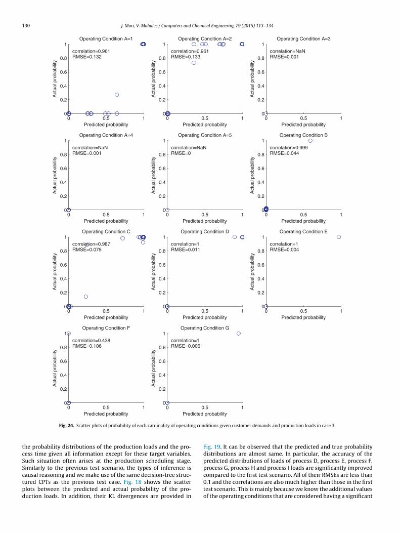
or comparison to the prediction, we classify the test data intoroduction groups which contain plates that have the sameustomer specifications and operating conditions and then com-ute the probability distribution for each production group. Theroduction groups containing more than 100 plates are chosen foromparison while the other production groups are not selectedecause we cannot compute the reliable probability distribu-ions from a small number of samples. The total number of theroduction groups that are used for comparison is 106.
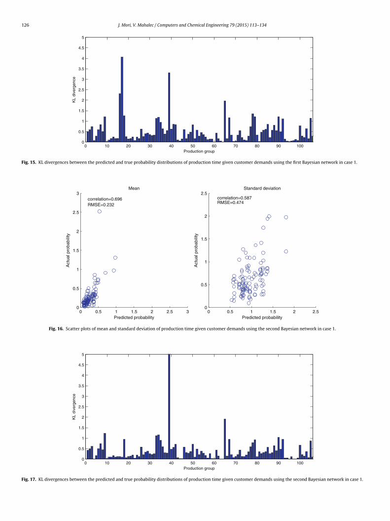
First, we predict the production loads and the productionime by using the first Bayesian network structure shown inig. 10. Fig. 12 shows the scatter plots between the predictednd true probabilities with production loads being 2. Further, theullback–Leibler (KL) divergence, which measures the differenceetween the predicted probability distributions and actual ones ishown in Fig. 13. It can be observed that the difference betweenhe predicted and true probability distributions of the variablesf process A, process B, process C, process D, process E, process Fnd process G are relatively small while the predicted probabilities
ith process H and process I values being 2 are zero in all pro-uction groups. Moreover, the scatter plots between the predictednd true parameters of means and standard deviations of the pro-uction time are shown in Fig. 14, and their KL divergences areprobability Predicted probability
customer demands and operating conditions in case 2.
provided in Fig. 15. It can be seen that the means of the predicteddistributions are relatively close to the true means but the vari-ances of the predicted distributions largely differ from the actualones. Somewhat inaccurate prediction of the production loads ofprocess E, process F, process H and process I can be considered acause of these differences in the production time.
Next, the probability distributions of the production loads andthe production time are computed via the second type of Bayesiannetwork, shown in Fig. 11. The difference between the two struc-tures is that the nodes associated with the production time at eachproduction process are added between the nodes of productionloads and total production time in the second type on Bayesiannetwork. Similarly to the first model, we provide the scatter plotsof the predicted and true parameters of means and standard devi-ations and their KL divergences in Figs. 16 and 17, respectively. Itcan be observed that the prediction accuracy does not improve atall from the first Bayesian network. The cause of inaccurate predic-tion of the variances of the total production time is the low accurateprediction of the production loads.
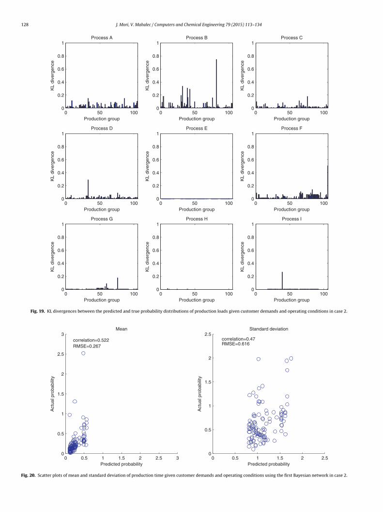
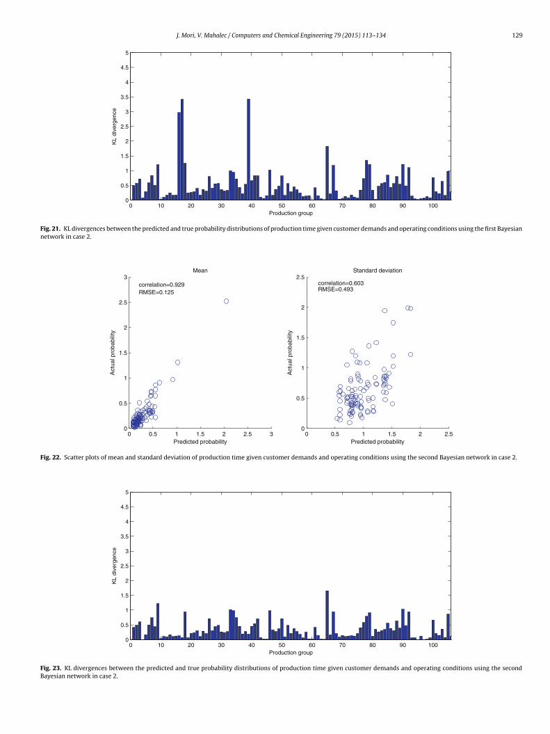
In the second test case, we consider the situation where thevariables associated with both customer demands and operatingconditions are known and the variables of both production loadsand process time are unknown. In this situation, we want to predict
128 J. Mori, V. Mahalec / Computers and Chemical Engineering 79 (2015) 113–134
0 50 1000
0.2
0.4
0.6
0.8
1Process A
Production group
KL
dive
rgen
ce
0 50 1000
0.2
0.4
0.6
0.8
1Process B
Production group
KL
dive
rgen
ce
0 50 1000
0.2
0.4
0.6
0.8
1Process C
Production group
KL
dive
rgen
ce
0 50 1000
0.2
0.4
0.6
0.8
1Process D
Production group
KL
dive
rgen
ce
0 50 1000
0.2
0.4
0.6
0.8
1Process E
Production group
KL
dive
rgen
ce
0 50 1000
0.2
0.4
0.6
0.8
1Process F
Production group
KL
dive
rgen
ce
0 50 1000
0.2
0.4
0.6
0.8
1Process G
Production group
KL
dive
rgen
ce
0 50 1000
0.2
0.4
0.6
0.8
1Process H
Production group
KL
dive
rgen
ce
0 50 1000
0.2
0.4
0.6
0.8
1Process I
Production group
KL
dive
rgen
ce
Fig. 19. KL divergences between the predicted and true probability distributions of production loads given customer demands and operating conditions in case 2.
0 0.5 1 1.5 2 2.5 30
0.5
1
1.5
2
2.5
3correlation=0.522RMSE=0.267
Mean
Predicted probability
Act
ual p
roba
bilit
y
0 0.5 1 1.5 2 2.50
0.5
1
1.5
2
2.5correlation=0.47RMSE=0.616
Standard deviation
Predicted probability
Act
ual p
roba
bilit
y
Fig. 20. Scatter plots of mean and standard deviation of production time given customer demands and operating conditions using the first Bayesian network in case 2.
J. Mori, V. Mahalec / Computers and Chemical Engineering 79 (2015) 113–134 129
0 10 20 30 40 50 60 70 80 90 1000
0.5
1
1.5
2
2.5
3
3.5
4
4.5
5
Production group
KL
dive
rgen
ce
Fig. 21. KL divergences between the predicted and true probability distributions of production time given customer demands and operating conditions using the first Bayesiannetwork in case 2.
0 0.5 1 1.5 2 2.5 30
0.5
1
1.5
2
2.5
3correlation=0.929RMSE=0.125
Mean
Predicted probability
Act
ual p
roba
bilit
y
0 0. 5 1 1. 5 2 2. 50
0.5
1
1.5
2
2.5correlation=0.603RMSE=0.493
Standard deviation
Predicted probability
Act
ual p
roba
bilit
y
Fig. 22. Scatter plots of mean and standard deviation of production time given customer demands and operating conditions using the second Bayesian network in case 2.
0 10 20 30 40 50 60 70 80 90 1000
0.5
1
1.5
2
2.5
3
3.5
4
4.5
5
Production group
KL
dive
rgen
ce
Fig. 23. KL divergences between the predicted and true probability distributions of production time given customer demands and operating conditions using the secondBayesian network in case 2.
130 J. Mori, V. Mahalec / Computers and Chemical Engineering 79 (2015) 113–134
0 0.5 10
0.2
0.4
0.6
0.8
1correlation=0.961RMSE=0.132
Operating Condition A=1
Predicted probability
Act
ual p
roba
bilit
y
0 0.5 10
0.2
0.4
0.6
0.8
1correlation=0.961RMSE=0.133
Operating Condition A=2
Predicted probability
Act
ual p
roba
bilit
y
0 0.5 10
0.2
0.4
0.6
0.8
1correlation=NaNRMSE=0.001
Operating Condition A=3
Predicted probability
Act
ual p
roba
bilit
y
0 0.5 10
0.2
0.4
0.6
0.8
1correlation=NaNRMSE=0.001
Operating Condition A=4
Predicted probability
Act
ual p
roba
bilit
y
0 0.5 10
0.2
0.4
0.6
0.8
1correlation=NaNRMSE=0
Operating Condition A=5
Predicted probability
Act
ual p
roba
bilit
y
0 0.5 10
0.2
0.4
0.6
0.8
1correlation=0.999RMSE=0.044
Operating Condition B
Predicted probability
Act
ual p
roba
bilit
y
0 0.5 10
0.2
0.4
0.6
0.8
1correlation=0.987RMSE=0.075
Operating Condition C
Predicted probability
Act
ual p
roba
bilit
y
0 0.5 10
0.2
0.4
0.6
0.8
1correlation=1RMSE=0.011
Operating Condition D
Predicted probability
Act
ual p
roba
bilit
y
0 0.5 10
0.2
0.4
0.6
0.8
1correlation=1RMSE=0.004
Operating Condition E
Predicted probability
Act
ual p
roba
bilit
y
0 0.5 10
0.2
0.4
0.6
0.8
1correlation=0.438RMSE=0.106
Operating Condition F
Predicted probability
Act
ual p
roba
bilit
y
0 0.5 10
0.2
0.4
0.6
0.8
1correlation=1RMSE=0.006
Operating Condition G
Predicted probability
Act
ual p
roba
bilit
y
g con
tcSSctpd
Fig. 24. Scatter plots of probability of each cardinality of operatin
he probability distributions of the production loads and the pro-ess time given all information except for these target variables.uch situation often arises at the production scheduling stage.imilarly to the previous test scenario, the types of inference is
ausal reasoning and we make use of the same decision-tree struc-ured CPTs as the previous test case. Fig. 18 shows the scatterlots between the predicted and actual probability of the pro-uction loads. In addition, their KL divergences are provided inditions given customer demands and production loads in case 3.
Fig. 19. It can be observed that the predicted and true probabilitydistributions are almost same. In particular, the accuracy of thepredicted distributions of loads of process D, process E, process F,process G, process H and process I loads are significantly improved
compared to the first test scenario. All of their RMSEs are less than0.1 and the correlations are also much higher than those in the firsttest scenario. This is mainly because we know the additional valuesof the operating conditions that are considered having a significant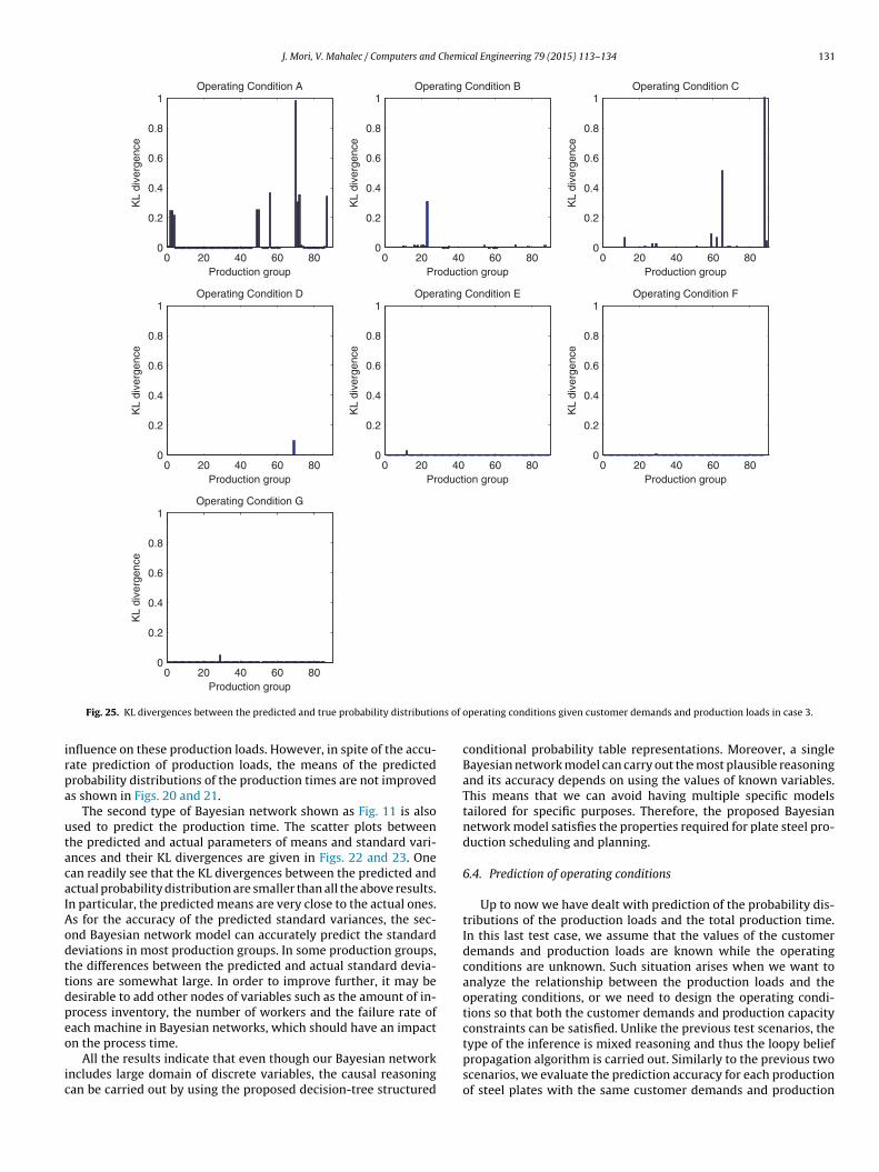
J. Mori, V. Mahalec / Computers and Chemical Engineering 79 (2015) 113–134 131
0 20 40 60 800
0.2
0.4
0.6
0.8
1
Production group
KL
dive
rgen
ce
Operating Condition A
0 20 40 60 800
0.2
0.4
0.6
0.8
1
Production group
KL
dive
rgen
ce
Operating Condition B
0 20 40 60 800
0.2
0.4
0.6
0.8
1
Production group
KL
dive
rgen
ce
Operating Condition C
0 20 40 60 800
0.2
0.4
0.6
0.8
1
Production group
KL
dive
rgen
ce
Operating Condition D
0 20 40 60 800
0.2
0.4
0.6
0.8
1
Production group
KL
dive
rgen
ce
Operating Condition E
0 20 40 60 800
0.2
0.4
0.6
0.8
1
Production group
KL
dive
rgen
ce
Operating Condition F
0 20 40 60 800
0.2
0.4
0.6
0.8
1
KL
dive
rgen
ce
Operating Condition G
ns of o
irpa
utacaIAodttdpeo
ic
Production group
Fig. 25. KL divergences between the predicted and true probability distributio
nfluence on these production loads. However, in spite of the accu-ate prediction of production loads, the means of the predictedrobability distributions of the production times are not improveds shown in Figs. 20 and 21.
The second type of Bayesian network shown as Fig. 11 is alsosed to predict the production time. The scatter plots betweenhe predicted and actual parameters of means and standard vari-nces and their KL divergences are given in Figs. 22 and 23. Onean readily see that the KL divergences between the predicted andctual probability distribution are smaller than all the above results.n particular, the predicted means are very close to the actual ones.s for the accuracy of the predicted standard variances, the sec-nd Bayesian network model can accurately predict the standardeviations in most production groups. In some production groups,he differences between the predicted and actual standard devia-ions are somewhat large. In order to improve further, it may beesirable to add other nodes of variables such as the amount of in-rocess inventory, the number of workers and the failure rate ofach machine in Bayesian networks, which should have an impact
n the process time.All the results indicate that even though our Bayesian networkncludes large domain of discrete variables, the causal reasoningan be carried out by using the proposed decision-tree structured
perating conditions given customer demands and production loads in case 3.
conditional probability table representations. Moreover, a singleBayesian network model can carry out the most plausible reasoningand its accuracy depends on using the values of known variables.This means that we can avoid having multiple specific modelstailored for specific purposes. Therefore, the proposed Bayesiannetwork model satisfies the properties required for plate steel pro-duction scheduling and planning.
6.4. Prediction of operating conditions
Up to now we have dealt with prediction of the probability dis-tributions of the production loads and the total production time.In this last test case, we assume that the values of the customerdemands and production loads are known while the operatingconditions are unknown. Such situation arises when we want toanalyze the relationship between the production loads and theoperating conditions, or we need to design the operating condi-tions so that both the customer demands and production capacityconstraints can be satisfied. Unlike the previous test scenarios, the
type of the inference is mixed reasoning and thus the loopy beliefpropagation algorithm is carried out. Similarly to the previous twoscenarios, we evaluate the prediction accuracy for each productionof steel plates with the same customer demands and production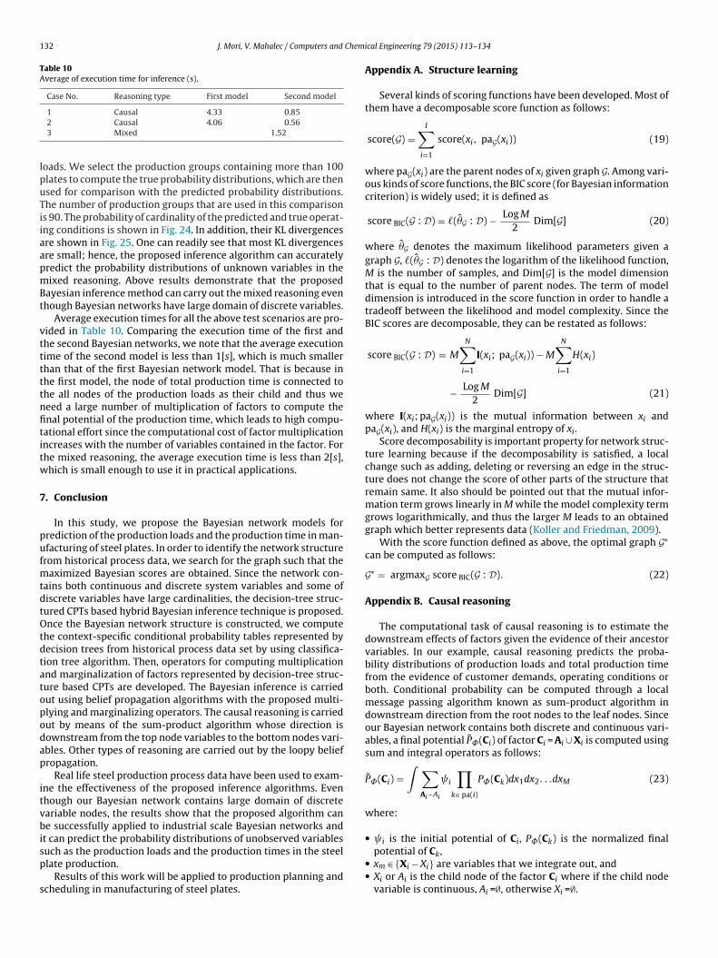
132 J. Mori, V. Mahalec / Computers and Chem
Table 10Average of execution time for inference (s).
Case No. Reasoning type First model Second model
1 Causal 4.33 0.85
lpuTiiaapmBt
vtttttnfititw
7
pufmtdtOtdtatopodap
itvbisp
s
2 Causal 4.06 0.563 Mixed 1.52
oads. We select the production groups containing more than 100lates to compute the true probability distributions, which are thensed for comparison with the predicted probability distributions.he number of production groups that are used in this comparisons 90. The probability of cardinality of the predicted and true operat-ng conditions is shown in Fig. 24. In addition, their KL divergencesre shown in Fig. 25. One can readily see that most KL divergencesre small; hence, the proposed inference algorithm can accuratelyredict the probability distributions of unknown variables in theixed reasoning. Above results demonstrate that the proposed
ayesian inference method can carry out the mixed reasoning evenhough Bayesian networks have large domain of discrete variables.
Average execution times for all the above test scenarios are pro-ided in Table 10. Comparing the execution time of the first andhe second Bayesian networks, we note that the average executionime of the second model is less than 1[s], which is much smallerhan that of the first Bayesian network model. That is because inhe first model, the node of total production time is connected tohe all nodes of the production loads as their child and thus weeed a large number of multiplication of factors to compute thenal potential of the production time, which leads to high compu-ational effort since the computational cost of factor multiplicationncreases with the number of variables contained in the factor. Forhe mixed reasoning, the average execution time is less than 2[s],hich is small enough to use it in practical applications.
. Conclusion
In this study, we propose the Bayesian network models forrediction of the production loads and the production time in man-facturing of steel plates. In order to identify the network structurerom historical process data, we search for the graph such that the
aximized Bayesian scores are obtained. Since the network con-ains both continuous and discrete system variables and some ofiscrete variables have large cardinalities, the decision-tree struc-ured CPTs based hybrid Bayesian inference technique is proposed.nce the Bayesian network structure is constructed, we compute
he context-specific conditional probability tables represented byecision trees from historical process data set by using classifica-ion tree algorithm. Then, operators for computing multiplicationnd marginalization of factors represented by decision-tree struc-ure based CPTs are developed. The Bayesian inference is carriedut using belief propagation algorithms with the proposed multi-lying and marginalizing operators. The causal reasoning is carriedut by means of the sum-product algorithm whose direction isownstream from the top node variables to the bottom nodes vari-bles. Other types of reasoning are carried out by the loopy beliefropagation.
Real life steel production process data have been used to exam-ne the effectiveness of the proposed inference algorithms. Evenhough our Bayesian network contains large domain of discreteariable nodes, the results show that the proposed algorithm cane successfully applied to industrial scale Bayesian networks and
t can predict the probability distributions of unobserved variables
uch as the production loads and the production times in the steellate production.Results of this work will be applied to production planning andcheduling in manufacturing of steel plates.
ical Engineering 79 (2015) 113–134
Appendix A. Structure learning
Several kinds of scoring functions have been developed. Most ofthem have a decomposable score function as follows:
score(G) =I∑i=1
score(xi, paG(xi)) (19)
where paG(xi) are the parent nodes of xi given graph G. Among vari-ous kinds of score functions, the BIC score (for Bayesian informationcriterion) is widely used; it is defined as
score BIC(G : D) = �(̂G : D) − Log M
2Dim[G] (20)
where ̂G denotes the maximum likelihood parameters given agraph G, �(̂G : D) denotes the logarithm of the likelihood function,M is the number of samples, and Dim[G] is the model dimensionthat is equal to the number of parent nodes. The term of modeldimension is introduced in the score function in order to handle atradeoff between the likelihood and model complexity. Since theBIC scores are decomposable, they can be restated as follows:
score BIC(G : D) = M
N∑i=1
I(xi; paG(xi)) − M
N∑i=1
H(xi)
− Log M
2Dim[G] (21)
where I(xi; paG(xi)) is the mutual information between xi andpaG(xi), and H(xi) is the marginal entropy of xi.
Score decomposability is important property for network struc-ture learning because if the decomposability is satisfied, a localchange such as adding, deleting or reversing an edge in the struc-ture does not change the score of other parts of the structure thatremain same. It also should be pointed out that the mutual infor-mation term grows linearly in M while the model complexity termgrows logarithmically, and thus the larger M leads to an obtainedgraph which better represents data (Koller and Friedman, 2009).
With the score function defined as above, the optimal graph G∗can be computed as follows:
G∗ = argmaxG score BIC(G : D). (22)
Appendix B. Causal reasoning
The computational task of causal reasoning is to estimate thedownstream effects of factors given the evidence of their ancestorvariables. In our example, causal reasoning predicts the proba-bility distributions of production loads and total production timefrom the evidence of customer demands, operating conditions orboth. Conditional probability can be computed through a localmessage passing algorithm known as sum-product algorithm indownstream direction from the root nodes to the leaf nodes. Sinceour Bayesian network contains both discrete and continuous vari-ables, a final potential P̃˚(Ci) of factor Ci = Ai ∪ Xi is computed usingsum and integral operators as follows:
P̃˚(Ci) =∫ ∑
Ai−Ai
i∏k∈ pa(i)
P˚(Ck)dx1dx2. . .dxM (23)
where:
• i is the initial potential of Ci, P˚(Ck) is the normalized final
potential of Ck,• xm ∈ {Xi− Xi} are variables that we integrate out, and• Xi or Ai is the child node of the factor Ci where if the child nodevariable is continuous, Ai =∅, otherwise Xi =∅.
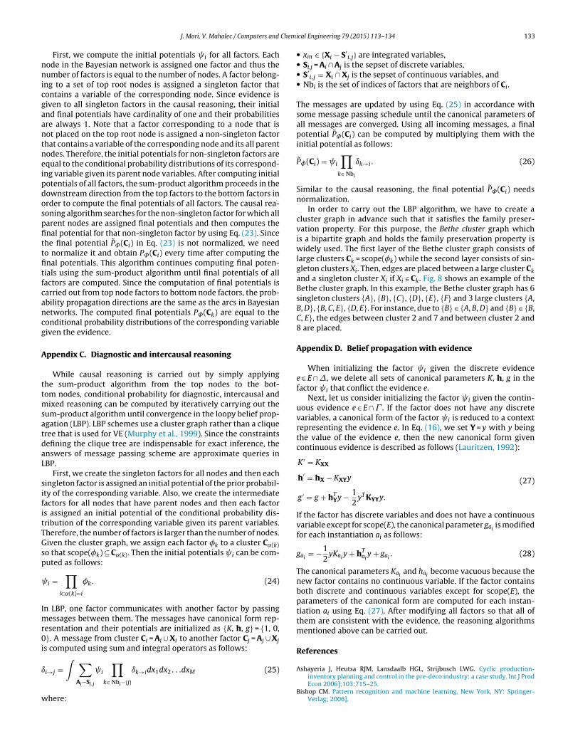
Chemi
nnicgaantneipdospfittfitfcancg
A
ttmsatdaL
sifitTGsp
Imr0i
ı
w
J. Mori, V. Mahalec / Computers and
First, we compute the initial potentials i for all factors. Eachode in the Bayesian network is assigned one factor and thus theumber of factors is equal to the number of nodes. A factor belong-
ng to a set of top root nodes is assigned a singleton factor thatontains a variable of the corresponding node. Since evidence isiven to all singleton factors in the causal reasoning, their initialnd final potentials have cardinality of one and their probabilitiesre always 1. Note that a factor corresponding to a node that isot placed on the top root node is assigned a non-singleton factorhat contains a variable of the corresponding node and its all parentodes. Therefore, the initial potentials for non-singleton factors arequal to the conditional probability distributions of its correspond-ng variable given its parent node variables. After computing initialotentials of all factors, the sum-product algorithm proceeds in theownstream direction from the top factors to the bottom factors inrder to compute the final potentials of all factors. The causal rea-oning algorithm searches for the non-singleton factor for which allarent nodes are assigned final potentials and then computes thenal potential for that non-singleton factor by using Eq. (23). Sincehe final potential P̃˚(Ci) in Eq. (23) is not normalized, we needo normalize it and obtain P˚(Ci) every time after computing thenal potentials. This algorithm continues computing final poten-ials using the sum-product algorithm until final potentials of allactors are computed. Since the computation of final potentials isarried out from top node factors to bottom node factors, the prob-bility propagation directions are the same as the arcs in Bayesianetworks. The computed final potentials P˚(Ck) are equal to theonditional probability distributions of the corresponding variableiven the evidence.
ppendix C. Diagnostic and intercausal reasoning
While causal reasoning is carried out by simply applyinghe sum-product algorithm from the top nodes to the bot-om nodes, conditional probability for diagnostic, intercausal and
ixed reasoning can be computed by iteratively carrying out theum-product algorithm until convergence in the loopy belief prop-gation (LBP). LBP schemes use a cluster graph rather than a cliqueree that is used for VE (Murphy et al., 1999). Since the constraintsefining the clique tree are indispensable for exact inference, thenswers of message passing scheme are approximate queries inBP.
First, we create the singleton factors for all nodes and then eachingleton factor is assigned an initial potential of the prior probabil-ty of the corresponding variable. Also, we create the intermediateactors for all nodes that have parent nodes and then each factors assigned an initial potential of the conditional probability dis-ribution of the corresponding variable given its parent variables.herefore, the number of factors is larger than the number of nodes.iven the cluster graph, we assign each factor k to a cluster C˛(k)o that scope(k) ⊆ C˛(k). Then the initial potentials i can be com-uted as follows:
i =∏
k:˛(k)=ik. (24)
n LBP, one factor communicates with another factor by passingessages between them. The messages have canonical form rep-
esentation and their potentials are initialized as {K, h, g} = {1, 0,}. A message from cluster Ci = Ai ∪ Xi to another factor Cj = Aj ∪ Xj
s computed using sum and integral operators as follows:∫ ∑ ∏
i→j =Ai−Si,j
ik∈ Nbi−{j}
ık→idx1dx2. . .dxM (25)
here:
cal Engineering 79 (2015) 113–134 133
• xm ∈ {Xi − S′i,j} are integrated variables,• Si,j = Ai ∩ Aj is the sepset of discrete variables,• S′i,j = Xi ∩ Xj is the sepset of continuous variables, and• Nbi is the set of indices of factors that are neighbors of Ci.
The messages are updated by using Eq. (25) in accordance withsome message passing schedule until the canonical parameters ofall messages are converged. Using all incoming messages, a finalpotential P̃˚(Ci) can be computed by multiplying them with theinitial potential as follows:
P̃˚(Ci) = i∏k∈ Nbi
ık→i. (26)
Similar to the causal reasoning, the final potential P̃˚(Ci) needsnormalization.
In order to carry out the LBP algorithm, we have to create acluster graph in advance such that it satisfies the family preser-vation property. For this purpose, the Bethe cluster graph whichis a bipartite graph and holds the family preservation property iswidely used. The first layer of the Bethe cluster graph consists oflarge clusters Ck = scope(k) while the second layer consists of sin-gleton clusters Xi. Then, edges are placed between a large cluster Ckand a singleton cluster Xi if Xi ∈ Ck. Fig. 8 shows an example of theBethe cluster graph. In this example, the Bethe cluster graph has 6singleton clusters {A}, {B}, {C}, {D}, {E}, {F} and 3 large clusters {A,B, D}, {B, C, E}, {D, E}. For instance, due to {B} ∈ {A, B, D} and {B} ∈ {B,C, E}, the edges between cluster 2 and 7 and between cluster 2 and8 are placed.
Appendix D. Belief propagation with evidence
When initializing the factor i given the discrete evidencee ∈ E ∩ �, we delete all sets of canonical parameters K, h, g in thefactor i that conflict the evidence e.
Next, let us consider initializing the factor i given the contin-uous evidence e ∈ E ∩ � . If the factor does not have any discretevariables, a canonical form of the factor i is reduced to a contextrepresenting the evidence e. In Eq. (16), we set Y = y with y beingthe value of the evidence e, then the new canonical form givencontinuous evidence is described as follows (Lauritzen, 1992):
K ′ = KXX
h′ = hX − KXYy
g′ = g + hTYy − 12yTKYYy.
(27)
If the factor has discrete variables and does not have a continuousvariable except for scope(E), the canonical parameter gai is modifiedfor each instantiation ai as follows:
gai = −12yKaiy + hTai y + gai . (28)
The canonical parameters Kai and hai become vacuous because thenew factor contains no continuous variable. If the factor containsboth discrete and continuous variables except for scope(E), theparameters of the canonical form are computed for each instan-tiation ai using Eq. (27). After modifying all factors so that all ofthem are consistent with the evidence, the reasoning algorithmsmentioned above can be carried out.
References
Ashayeria J, Heutsa RJM, Lansdaalb HGL, Strijbosch LWG. Cyclic production-inventory planning and control in the pre-deco industry: a case study. Int J ProdEcon 2006];103:715–25.
Bishop CM. Pattern recognition and machine learning. New York, NY: Springer-Verlag; 2006].
1 Chem
B
B
C
C
C
C
D
F
G
H
K
K
K
L
34 J. Mori, V. Mahalec / Computers and
outilier C, Friedman N, Goldszmidt M, Koller D. Context-specific independence inBayesian networks. In: Proceedings of UAI-96; 1996]. p. 115–23.
reiman L, Friedman JH, Olshen RA, Stone CG. Classification and regression trees.Belmont: Wadsworth International Group; 1984].
aputo B, Sim K, Furesjo F, Smola A. Appearance-based object recognition usingSVMs: which kernel should I use? In: Proceedings of NIPS workshop on Statisti-cal methods for computational experiments in visual processing and computervision; 2002].
hickering DM. Learning Bayesian networks is NP-complete. In: Learning from data:artificial intelligence and statistics. Springer-Verlag; 1996] [chapter 12].
hickering DM, Heckerman D, Meek C. A Bayesian approach to learning Bayesiannetworks with local structure. In: Proceedings of UAI-97; 1997]. p. 80–9.
obb BR, Rumi R, Salmeron A. Bayesian network models with discrete and continu-ous variables. Berlin: Springer-Verlag; 2007].
esJardins M, Rathod P. Learning structured Bayesian networks: combining abstrac-tion hierarchies and tree-structured conditional probability tables. ComputIntell 2008];24:1–22.
riedman N, Goldszmidt M. Learning Bayesian networks with local structure. In:Proceedings of UAI-96; 1996]. p. 252–62.
lover F. Future paths for integer programming and links to artificial intelligence.Comput Oper Res 1986];13:533–49.
arjunkoski I, Grossmann IE. A decomposition approach for the scheduling of a steelplant production. Comput Chem Eng 2001];25:1647–60.
oller D, Friedman N. Probabilistic graphical models: principles and techniques. MITPress; 2009].
oller D, Lerner U, Angelov D. A general algorithm for approximate inference and its
application to hybrid Bayes nets. In: Proceedings of UAI-99; 1999]. p. 324–33.ozlov A, Koller D. Nonuniform dynamic discretization in hybrid networks. In:Proceedings of UAI-97; 1997]. p. 314–25.
auritzen S. Propagation of probabilities, means and variances in mixed graphicalassociation models. J Am Stat Assoc 1992];87:1098–108.
ical Engineering 79 (2015) 113–134
Lauritzen SL, Jensen F. Stable local computation with conditional Gaussian distribu-tion. Stat Comput 2001];11:191–203.
Lauritzen SL, Wermuth N. Graphical models for associations between variables,some of which are qualitative and some quantitative. Ann Stat 1989];17:31–57.
Moon S, Hrymak AN. Scheduling of the batch annealing process-deterministic case.Comput Chem Eng 1999];23:1193–208.
Moral S, Rumi R, Salmeron A. Mixtures of truncated exponentials in hybrid Bayesiannetworks. Berlin: Springer-Verlag; 2001].
Murphy KP, Weiss Y, Jordan MI. Nonuniform dynamic discretization in hybridnetworks. In: Proceedings of UAI-99; 1999]. p. 467–75.
Nishioka K, Mizutani Y, Ueno H, Kawasaki H, Baba Y. Toward the integrated opti-mization of steel plate production process: a proposal for production control bymulti-scale hierarchical modeling. Synthesiology 2012];5:98–112 [in Japanese].
Pearl J. Probabilistic reasoning in intelligent systems: networks of plausible infer-ence. San Francisco: Morgan-Kaufmann; 1988].
Poole D, Zhang NL. Exploiting contextual independence in probabilistic inference. JArtif Intell Res 2003];18:263–313.
Rumi R, Salmeron A. Approximate probability propagation with mixtures of trun-cated exponentials. Int J Approx Reason 2007];45:191–210.
Santos CA, Spim JA, Garci A. Mathematical modeling and optimization strategies(genetic algorithm and knowledge base) applied to the continuous casting ofsteel. Eng Appl Artif Intel 2003];16:511–27.
Sharma R, Poole D. Efficient inference in large discrete domains. In: Proceedings ofUAI-2003; 2003]. p. 535–42.
Tang L, Liu J, Rong A, Yang Z. A mathematical programming model for sched-
uling steel making continuous casting production. Eur J Oper Res 2000];120:423–35.Yuan C, Druzdzel MJ. Hybrid loopy belief propagation. In: Proceedings of the thirdEuropean workshop on probabilistic graphical models (PGM’06); 2006]. p.317–24.