1-s2.0-S0021999108003343-main

Journal of Computational Physics 227 (2008) 8636–8654

Contents lists available at ScienceDirect

Journal of Computational Physics

journal homepage: www.elsevier .com/locate / jcp

An immersed boundary method for smoothed particlehydrodynamics of self-propelled swimmers

S.E. Hieber, P. Koumoutsakos *

Chair of Computational Science, Universitatstrasse 6, ETH Zurich, CH-8092 Zurich, Switzerland

a r t i c l e i n f o

Article history:Received 20 December 2007Received in revised form 12 June 2008Accepted 16 June 2008Available online 27 June 2008

Keywords:Particle MethodsSwimmingSPHImmersed Boundary Methods

0021-9991/$ - see front matter � 2008 Elsevier Incdoi:10.1016/j.jcp.2008.06.017

* Corresponding author. Tel.: +41 44 632 5258; faE-mail addresses: [email protected]

a b s t r a c t

We present a novel particle method, combining remeshed Smoothed Particle Hydrody-namics with Immersed Boundary and Level Set techniques for the simulation of flows pastcomplex deforming geometries. The present method retains the Lagrangian adaptivity ofparticle methods and relies on the remeshing of particle locations in order to ensure theaccuracy of the method. In fact this remeshing step enables the introduction of ImmersedBoundary Techniques used in grid based methods. The method is applied to simulations offlows of isothermal and compressible fluids past steady and unsteady solid boundaries thatare described using a particle Level Set formulation. The method is validated with two andthree-dimensional benchmark problems of flows past cylinders and spheres and it isshown to be well suited to simulations of large scale simulations using tens of millionsof particles, on flow-structure interaction problems as they pertain to self-propelledanguilliform swimmers.

� 2008 Elsevier Inc. All rights reserved.

1. Introduction

The efficient and accurate simulation of fluid flows interacting with complex deforming geometries is of paramountimportance to a number of scientific fields ranging from virtual surgery to biofluid dynamics. These simulations require flowsolvers capable of handling accurately complex geometries and resolving efficiently the details of the flow field. In grid basedmethods a number of techniques, have been developed to address such problems distinguished by their handling of the solidgeometry embedded in the flow field. Unstructured grid methods [15] are widely used techniques employing sets of gridsthat adapt to the deformation of the boundary. The advantages of these methods relies on the accuracy of the flow solvernear boundaries and their flexibility in handling highly complex geometries. On the other hand, in particular for deforminggeometries, these methods require an additional computational cost for constructing the grid anew at each time step andthey are often associated with an additional computational overhead in solving the governing equations due to the non-uni-formity of the associated mesh. Immersed Boundary Methods (IBM), pioneered by Peskin [39], use a straightforward bound-ary representation along with structured grids to discretize flows past complex deforming geometries without constructingthe grid anew at each time step. In IBM the effects of the boundary are accounted for by introducing a forcing term on thegoverning equations localized at the boundary of the body. These methods have attracted significant attention in recentyears for the simulation of complex flows in two and three-dimensions (see [34] and references therein).

Particle methods such as Vortex Methods (VM) and Smoothed Particle Hydrodynamics (SPH) are Lagrangian tech-niques that are widely considered as being capable of handling flows past complex deforming geometries. In fact wenote that the original development of Immersed Boundary Methods was in the context of VMs [39] for the simulationof heart leaflets at physiological Reynolds numbers. Building on the viscous VM introduced by Chorin [6], Peskin’s

. All rights reserved.

x: +41 44 632 1703.hz.ch (S.E. Hieber), [email protected] (P. Koumoutsakos).

mailto:[email protected]

mailto:[email protected]

http://www.sciencedirect.com/science/journal/00219991

http://www.elsevier.com/locate/jcp

S.E. Hieber, P. Koumoutsakos / Journal of Computational Physics 227 (2008) 8636–8654 8637

pioneering simulations, coupled IBM and VM in an effort to use a minimal set of computational points to capture thedynamics of the vorticity field in a complex deforming geometry. These simulations however were hindered at that timeby the quadratic cost of VMs and by the low accuracy associated with their treatment of viscous effects. Another issue,hidden in the Lagrangian description of the flow, is the inaccuracy of particle methods when the flow distorts the com-putational elements. The fact that VMs were able to provide reasonable estimates of force fields and flow structures (inparticular in 2D), but they were not capable of Direct Numerical Simulations of bluff body flows, detracted from theiroriginal success. Recent works introducing a regularization of the particle locations have rekindled and interest in thesemethods as being capable of performing Direct Numerical Simulations (see [29] and references therein), albeit only forflows past relatively simple boundaries.

Contemporary to the inception of VMs [6,31], Lucy [33] and Gingold and Monaghan [17] introduced the method ofSmoothed Particle Hydrodynamics to discretize the velocity–pressure formulation of the compressible Navier–Stokesequations. A key advantage of SPH is the avoidance of solving an elliptic problem to determine the velocity field ofthe flow by introducing a state equation linking the pressure and the density field of the flow. Over the years a largebody of work has implemented SPH for simulations of flows ranging from astrophysics, to polymer dynamics (see thereview by Monaghan [36] and references therein). The SPH method is inherently adaptive as particle attributes (strength,locations) evolve according to their material time derivatives. At the same time, the particle distortion, associated withall Lagrangian particle methods, often leads to large inaccuracies of the quantities that are been simulated. In order tocircumvent this problem a consistent framework involving remeshing of particle locations using moment conservingschemes was introduced in [30]. The moment conserving remeshing schemes developed in [27], were inspired in factby SPH interpolations [17], and they have been in turn applied in the context of SPH resulting in the method of re-meshed SPH (rSPH) [5]. In the rSPH the particles are reinitialized (remeshing) on a regular grid and the new particlestrengths are adjusted so that the moments of the field quantities are conserved. We emphasize that the combinationof meshes and particle does not detract from the adaptive character of the method as the nonlinear convection termis still described in a Lagrangian fashion. Care must be exercised however when remeshing near boundaries so as notto introduce spurious structures while conserving the moments of the flow. This remeshing difficulty can be overcomeby combining Immersed Boundary Methods and the rSPH as shown in this work.

In IBM the effects of the boundary to the flow are accounted for by adding a forcing term to the governing equations[40,42,41]. This forcing term is computed so as to enforce the no-slip boundary condition on the surface of the body. Theequations are usually discretized on an Eulerian grid which does not need to coincide with the location of the body and aforcing term has to be computed on the grid nodes in the vicinity of the boundary. Fadlun et al. [14] proposed an IBM forfinite-difference methods where the velocity field for grid points near the boundary is interpolated linearly from valuesat the boundary leading to a second order accuracy for the overall method. Kim [26] presented a similar approach for fi-nite-volume methods combined with a mass source to increase the accuracy of the simulations.

These approaches have been so far mostly limited to Eulerian methods for incompressible flows. In the context ofparticle methods recent works by Cottet and Maitre [10] and Morgenthal and Walther [37] combined VMs with im-mersed interface and immersed boundary methods. Furthermore the IBM technique has been coupled with the Repro-ducing Kernel Methods [49] while in [12] Immersed Boundary techniques were combined with Lattice Boltzmannsimulations.

In this work we present a novel particle Immersed Boundary method for simulations using remeshed Smoothed ParticleHydrodynamics (rSPH-IB). The geometry of the body is described by Lagrangian particle level sets [21] and a forcing term isevaluated on the boundary points such that the no-slip boundary condition on the body is fulfilled. The extrapolation of theforcing term onto the neighboring particles employs a high-order B-Spline kernel. The method is applied to simulations offlows of self-propelled anguiliform swimmers. In this flow-structure interaction problem the fluid forces are taken into ac-count in order to determine the translation and rotation of the body. Anguilliform swimmers propel themselves by undula-tions that propagate along the entire length of the body and their simulation requires the continuous adaptation of thecomputational elements that describe the flow field. This is precisely the scope of the proposed method and we compareour result with related simulations [25] employing finite volume discretisations.

The paper is organized as follows. First, we present the governing equations in Section 2 and discuss the particle repre-sentation of Immersed Boundaries in Section 3. In Section 4, we demonstrate the performance of the rSPH-IB method onPoiseuille flow, flow past a circular cylinder and sphere. We compare the characteristic numbers of the flow for various Rey-nolds numbers with experimental and numerical results presented in the literature. Section 5 involves the simulation offluid-structure interactions describing a self-propelled swimmer. We conclude in Section 6 and discuss advantages and lim-itations of the present approach and outline future work.

2. Governing equations

We consider the isothermal, compressible Navier–Stokes equations, described in a non-dimensional Lagrangian, velocity–pressure framework as

DqDt¼ �qr � u; ð1Þ

8638 S.E. Hieber, P. Koumoutsakos / Journal of Computational Physics 227 (2008) 8636–8654

qDuDt¼ � 1

M2crpþ 1

Rer � s; ð2Þ

sij ¼ l oui

oxjþ ouj

oxi� 2

3dij

ouk

oxk

� �ð3Þ

where D}Dt ¼

o}ot þ ðu � rÞð}Þ denotes the material derivative, q denotes the density, u the velocity, p the pressure, s the shear

stress tensor with the elements sij, xi are the components of the position, ui the components of the velocity where Einstein’ssummation convention must be taken into account. The Reynolds number Re of the flow is defined as

Re ¼ q0Udl

; ð4Þ

where q0 is the characteristic density of fluid, U the characteristic velocity, l the dynamic viscosity and d is the characteristiclength of the boundary. The Mach number M is the ratio of the characteristic velocity U to the speed of sound c0

M ¼ Uc0¼ Uffiffiffiffiffiffiffiffi

RT0p : ð5Þ

The system of differential equations Eqs. (1)–(3) is closed by introducing equation of state for an ideal gas

p ¼ qT ð6Þ

where T is the temperature. In the present work we assume the temperature T ¼ T0 to be constant in space and time.The initial condition of the flow is described by a density and a velocity field. The no-slip boundary condition is translated

into a body force for the fluid in the vicinity of the body in the context of the immersed boundary technique. The inflowboundary involves a prescribed inlet velocity and a homogenous Neumann boundary condition for the pressure. At the out-let, we prescribe the pressure field and use a homogenous Neumann boundary condition for the velocity. Periodic boundaryconditions are employed in the remaining boundaries of the computational domain.

3. Re-meshed particle methods and immersed boundaries

3.1. Function and gradient approximations using particles

In the context of particle methods [18,8] a smooth approximation of a function UðxÞ is constructed by using a mollifica-tion kernel f�ðxÞ:

U�ðxÞ ¼ UHf� ¼Z

UðyÞf�ðx� yÞdy ð7Þ

where � denotes a characteristic length of the kernel.The mollification accuracy of this kernel is of order r when the following moment conditions [8] are satisfied:
Z
f�ðxÞdx ¼ 1; ð8ÞZxif�ðxÞdx ¼ 0 if j i j6 r � 1; ð9ÞZj xjrf�ðxÞdx 61: ð10Þ

This mollified approximation U�ðxÞ is discretised using the particle locations as quadrature points and a particle approxima-tion of the regularized function is

Uh�ðxÞ ¼ Uh

Hf� ¼XN

p¼1

vpUpf�ðx� xpÞ; ð11Þ

where xp, and vp denote the position and volume of the pth particle, and Up ¼ UðxpÞ the value at the p ¼ 1; � � � ;N particlelocations.

The error introduced by the quadrature of the mollified approximation of U can be distinguished in two parts [8] as

U�Uh� ¼ ðU�UHf�Þ þ ðU�UhÞHf�: ð12Þ

The first term in Eq. (12) denotes the mollification error that can be controlled by appropriately selecting the kernel prop-erties. The second term denotes the quadrature error due to the approximation of the integral on the particle locations. Theoverall accuracy of the method [8] results in

kU�Uh�k0;p 6 kU�U�k0;p þ kU� �Uh

�k0;p � Oð�rÞ þ Ohm

�m

� �; ð13Þ


where kð:Þk0;p ¼ ðRð:ÞpdxÞ1=p and r denotes the order of the first non-vanishing moment of the kernel f� [8]. For equidistant

particle locations m ¼ 1 and for positive kernels such as the Gaussian, r ¼ 2. Here for f� a quartic spline kernel with secondorder of accuracy is implemented

f�ðxÞ ¼ ndf� ¼ nd

s4

4 � 5s2

8 þ 115192 0 6 s < 1

2 ; s ¼ jxj� ;� s4

6 þ 5s3

6 � 5s2

4 þ 5s24þ 55

9612 6 s < 3

2 ;

ð2:5�sÞ424

32 6 s < 5

2 ;

0 s P 52 :

8>>>>><>>>>>:

ð14Þ

The normalization value nd depends on the dimension of the problem and is computed as

nd ¼1P

jvjf�ðx� xjÞð15Þ

ensuring the property of partition of unity for the particles. Kernels of arbitrary order [1] are possible by giving up the pos-itivity of the kernel function. Note that the moment conditions expressed by the integrals of the mollifier functions are notoften well represented in the case of discrete particle sets but the moment conditions can be ensured by appropriate nor-malisations [8].

The error estimates reveal a very important fact for smooth particle approximations. In order to obtain accurate approx-imations of the discretized quantities, smooth particles must overlap. This fact must be taken into account when consideringparticle simulations with Lagrangian adaptivity as the flow map often results in distortion of the computational elements,thus making the simulations inaccurate. This observation leads to the requirement for a regularization of the particle loca-tions which in turn may seem as detracting from the adaptive character of the method. As it is noted below this is not thecase as the regularization of the particle locations can be achieved by introducing less error than that introduced by particlemollification by appropriately conserving the moments of the flow field.

3.2. Remeshing

A key aspect of the present method involves the a remeshing procedure. In smooth particle methods, as discussed earlier,particles must overlap at all times in order to guarantee the convergence of the method [9]. As it is shown in [7] remeshing isequivalent to a regularisation of the advected quantities.

In this work remeshing is employed in order to regularize the distorted particle locations and to redistribute particlequantities accordingly onto a uniform set of particles with the spacing h.

The redistribution of particle quantities is achieved using the 3rd order M04 kernel [28] which in one dimension is ex-pressed as

M04ðx;hÞ ¼

1� 5s2

2 þ 3s3

2 0 6 s < 1; s ¼ jxjhð1�sÞð2�sÞ2

2 1 6 s < 2;0 s P 2:

8>><>>: ð16Þ

In higher dimensions the interpolation formulas are tensorial products of their one-dimensional counterparts. This reme-shing kernel is used in order to redistribute on regularised particle locations the discretized extensive properties (here massand momentum) of the field that need to be conserved.

In the context of SPH, remeshing requires a normalization scheme of the remeshed quantities in terms of theparticle volumes. The normalization scheme is similar to the normalization that ensures the partition of unity(Eq. (15)).

Uj;new ¼VnewPNold

i¼1VoldM04ðj xi � xj j;hÞ

XNold

i¼1Ui;oldM04ðj xi � xj j;hÞ; ð17Þ

where Vnew ¼ h3 is the volume of the new particle.After remeshing the new regularized particles are ready to be advected with the flow field. We note that this method does

not detract from the Lagrangian character of the method as the remeshing step is only seen as a regularization step for theparticle locations that are always advected by the flow map.

3.2.1. Particle derivative approximationsParticle approximations of the derivative operators can be constructed through their integral approximations. This can be

achieved by taking the derivatives of Eq. (7) as convolution and derivative operators commute in unbounded or periodic do-mains. This approximation is often employed in SPH [35] where derivatives of a field quantity U on a particle p are approx-imated in a conservative form as

Fig. 1.kernel


o

oxiU

� �p¼X

q

vqðUq �UpÞo

oxif�ðxp � xqÞ; ð18Þ

o

oxixjU

� �p

¼X

q

vqðUq �UpÞo

oxixjf�ðxp � xqÞ; ð19Þ

where vq is the volume of particle q. The normalization values nd;1;nd;2 of ooxi

f�ðxÞ ¼ nd;1o

oxif�ðxÞ and o

oxixjf�ðxÞ ¼ nd;2

ooxixj

f�ðxÞ are

chosen such that the corresponding non-zero moment condition [13] is satisfied. The kernel of Eq. (14) has its first threederivatives continuous allowing a smooth approximation of the spatial derivatives of UðxÞ. The computation of the righthand side of the ODEs employs these formulas for the computation of derivatives as defined in Eqs. (1)–(3). An alternativeformulation involves the development of integral operators that are equivalent to differential operators [13] as they werefirst introduced for the integral approximation of the Laplacian [11] in the diffusion equation.

3.3. An immersed boundary method for remeshed SPH

In rSPH-IB, (Fig. 1), a forcing term f is added to the momentum equation (Eq. (2)) such that the no-slip condition is sat-isfied on the boundary.

qDuDt¼ � 1

M2crpþ 1

Rer � sþ f : ð20Þ

We approximate the material derivative by a differential quotient:

qiuiþ1 � ui

Dt¼ � 1

M2crpi þ

1Rer � si þ fi ð21Þ

Solving for fi and assuming we reach the desired velocity within this time step (uiþ1 ¼ udesired) yields

fi ¼ qiudesired � ui

Dt� � 1

M2crpi þ

1Rer � si

!: ð22Þ

The forcing term f acts locally on the boundaries where a no-slip condition is imposed and the velocity udesired is known. Wenote that for the simulations past stationary boundaries, conducted in this study, the dominant contribution (90%) to theforcing term is due to the first term of Eq. (22), ‘‘correcting” the spurious velocity field at the boundary.

The boundary is described by boundary points associated in turn with an impact zone in the flow domain as determinedby the particle-mesh interpolations necessary for the transfer of the forcing term between the fluid and the body (Fig. 1). Weemploy a kernel based on B-Splines for a dirac delta approximation of the forcing term f. We rely on particle-mesh and mesh-particle interpolations, similar to those employed for remeshing in order to transport quantities between the fluid particlesand the boundary.

Our implementation involves the separation of the forcing term into two parts:

fi ¼ qiðfip þ fibÞ ð23Þ

fip ¼�ui

Dt� 1

qi� 1

M2crpi þ

1Rer � si

!ð24Þ

fib ¼udesired

Dtð25Þ

Particle Immersed Boundary Method. The immersed boundary is discretized using boundary points that can only impact flow particles within thesupport.


The rSPH-IB method consists the following steps:

1. Evaluation of the first part of the forcing term fip on the particle2. Interpolation of fip from the particles onto the boundary points via mesh.3. Evaluate forcing term fi on the boundary points by adding fib

4. Interpolation of forcing term f from the boundary points to the particles via mesh.5. Evolving particles according to the governing equations including forcing term f.

This approach tends to exhibit small scale oscillations in the pressure profile at complex boundaries. These oscillationscan be limited by the adjustment the density in the vicinity of the body. In this context, the ghost particles reside at theboundary and their density is here chosen to be the averaged density of the neighboring fluid particles within their support.

3.4. Particle equations

The particle position xp, mass mp, volume vp, and velocity component ui;p evolve by the following system of ordinary dif-ferential equations derived from Eqs. ((1)–(3))

dxp

dt¼ up

dmp

dt¼ 0

dvp

dt¼ hr � uipvp

dui;p

dt¼ vp

mp� 1

M2chopoxiip þ

1Rehosij

oxjip

!þ fi;p ð26Þ

where h}ip denotes the derivative approximation on a particle p (cf. Eq. (18)) and

osij

oxj

� �p

¼ l o2ui

ox2k

* +p

þ 13

o2ul

oxioxl

* +p

0@

1A ð27Þ

pp ¼mp

vpT0 ð28Þ

In the present study, the Laplacian approximation o2uiox2

k

� �p

is evaluated using the particle strength exchange approach [11].* +
o2ui
ox2k p

¼X

p

vpðui;p � ui;qÞr2f�ðxq � xpÞ ð29Þ

f� ¼15��3p

1

j xj10 þ 1ð30Þ

The second order kernel f� was successfully applied in simulations of diffusion in complex geometries [47].The interface between the body and the fluid is captured using the Particle Level Set Method [21,20]. The level set func-

tion represents the signed distance function to the interface. The particles carry the level set information as a scalar attributeUp that remains constant during the time integration:

dUp

dt¼ 0 ð31Þ

We reinitialize the level set value based on the prescribed deformation of the geometry after every remeshing to maintainthe signed distance property. The exact knowledge of the body shape allows the reinitialization of the level set function withits analytical value. We note that the use of the Level Set formulation enables the extension of the method to complexdeforming geometries that may even undergo topological changes that is of interest to virtual surgery applications.

The inlet and outlet boundary conditions are imposed by using image particles that have similar physical properties asthe flow particles. The boundary particles interact with the flow particles such that the boundary conditions are satisfied.The no-slip boundary condition on the body surface is handled by the proposed particle Immersed Boundary Method.

The implementation is embedded into the framework of the Parallel Particle-Mesh Library (PPM) [47] to perform large-scale simulations on massively parallel computer architectures.

4. Results

We implement the proposed rSPH-IB method on simulations of several benchmark flow problems, and present resultssuch as drag coefficient and vorticity isosurfaces. We discuss the advantages and drawbacks of the present method and


we demonstrate its capabilities in capturing flows past unsteady deforming geometries in simulations of flows past a self-propelled anguilliform swimmer.

The flows are characterized by their Reynolds and Mach numbers as defined in Section 2. The drag and lift coefficient aredefined as

Fig

ðCd;CLÞ ¼ðFD; FLÞ

0:5qU2A; ð32Þ

where FD; FL, demote the drag and lift force respectively on the body and A denotes the reference area. The Strouhal numberis defined as the dimensionless frequency of the shedding vortices

St ¼ fdU; ð33Þ

where f is the vortex shedding frequency, obtained using the Fast Fourier Transform of the lift coefficient.In order to perform effectively incompressible simulations, we have kept the Mach number to a minimum. On the other

hand, the low Mach number dictates a small time step for integrating the governing equations. We have chosen the Machnumber empirically so as to have a compromise between these two objectives.

4.1. Poiseuille flow

In order to verify the capability of the present method to capture flows past solid boundaries we consider first the Poiseu-ille flow. We note that this flow is a rather trivial example, in the context of grid based methods, but serves to demonstratethat the proposed particle-mesh framework allows for a straightforward simulation of such flows. The 2D simulation domainwas considered to be a unit square with periodic boundary condition at the inlet/outlet boundary (x = 0, x = 1) and no-slipconditions at the plates (y = 0, y = 1). We consider a fluid density with an initial density of q ¼ q0 ¼ 1 at a Reynolds numberof Re ¼ 100 and a Mach number of M ¼ 0:5. The fluid is initially at rest and accelerated by a constant pressure gradient of0.001. We employ a 2nd order Runge Kutta scheme with a time step of dt ¼ 0:0005 in all cases. For the error analysis themaximal difference in the velocity profile to the analytical solution is evaluated when the profile becomes stationary at timeT ¼ 70. The error normalized by the maximal velocity is shown in Fig. 2. The error analysis shows that the present methodexhibits second order accuracy in space.

4.2. Flow past a cylinder

We present simulations of flow past a cylinder for various Reynolds numbers using the proposed rSPH-IB in order to dem-onstrate the capability of the method to capture flows past non grid conforming boundaries and to compare the results of oursimulations with the related, benchmark experimental and computational investigations [19,26,32,38,45,48,50].

We use a 4th order Runge Kutta scheme for time integration with constant time step of Dt ¼ 0:001. The domain size is setto 15d� 30d where d is the diameter of the cylinder. The Mach number M is 0:05 The solution is remeshed after every timestep. A particle spacing of h ¼ 0:078d for Re ¼ 100 and h ¼ 0:052d for Re ¼ 1000 is employed in the reported simulations. Thefluid is initially at rest and accelerated by a small artificial force until the desired inlet velocity is reached to avoid the devel-opment of pressure waves at the boundary. The shedding is induced by a perturbation of the inlet velocity in the lateral

101

102

10−4

10−3

10−2

10−1

. 2. Poiseuille flow: L1� error velocity of the particle Immersed Boundary Method (rSPH-IB) compared to second order scaling (dashed line).

0 20 40 60 80 100 120 140 160 180−1.5

−1

−0.5

0

0.5

1

1.5

0 20 40 60 80 100 120 140 160 180−5.0

0.0

5.0

10.

15.0

20.0

0 20 40 60 80 100 120 140 160 1800

0.02

0.04

0.06

0.08

0.1

Fig. 3. Flow past a cylinder at Re ¼ 100: Effect of the resolution on wall quantities at t ¼ 2:5 before flow perturbation. The dashed, dash-dotted and solidlines represent particle spacings of h ¼ 0:156d, h ¼ 0:078d and h ¼ 0:039d, respectively.


direction as described by Ploumhans [44]. Fig. 3 shows the pressure coefficient, the vorticity and the forcing term along theboundary for three resolutions. In the region of high vorticity a high resolution is required to capture the boundary effects.This region also reflects a high forcing term. Furthermore we note the correlation of the forcing term with the the pressuregradient and the wall vorticity. Using Richardson’s extrapolation for the Euclidian norm of the wall vorticity we find that themethod converges with an order of 1.82.

Figs. 4 and 5 shows the vorticity field at Re ¼ 100 and Re ¼ 1000 respectively. These vorticity fields match qualitativelywell with the respective vorticity fields obtained via Finite Element solutions by Singh et al. [48].

Fig. 6 shows the variation of the drag coefficient with the Reynolds number. The simulation results of the rSPH-IBmethod are compared with experimental results [45] and incompressible flow computations. We observe that the dragcoefficient and Strouhal frequency values from present computations match well the experimental values for Re < 200

Fig. 4. Flow past a cylinder at Re ¼ 100. Contour levels of the vorticity contours at (�20;�15;�10;�7:5;�5;�2:5).

Fig. 5. Flow past a cylinder at Re ¼ 1000. Contour levels of the vorticity contours at (�20;�15;�10;�5).


and previous simulation results as listed on Table 1. Beyond Re ¼ 180 the wake flow undergoes three-dimensional tran-sitional instabilities. For Re > 200 the drag coefficient and the Strouhal number are overpredicted by the two-dimensionalcomputations.

Fig. 7 shows the pressure coefficient of the time averaged flow along the cylinder surface for Re ¼ 100 compared to theresult of Park et al. [38]. The angle h is measured clockwise from the front stagnation point of the cylinder. The pressurecoefficient Cp agrees well with the results of Park et al. [38]. The pressure field is noisy for angles 10� < h < 50� due tounresolved pressure waves in the compressible fluid.

Fig. 8 shows that the computational cost of the method scales linearly with the number of particles.

100

101

102

103

0

0.5

1

1.5

2

2.5

3

Fig. 6. Flow past a cylinder: Time averaged drag coefficient of rSPH-IB (circles) versus Reynolds number in comparison with experimental data (solid line,taken from Ref. [45]), a Spectral Method (dashed line, taken from Ref. [48]) and a FEM solution (crosses) [48].

Table 1Flow past a cylinder: comparison with previous simulations and experiments

Re ¼ 100;D ¼ 0:2 Drag coefficient Strouhal number

rSPH-IB 1.38 0.162Henderson [19] 1.35 –Park et al. [38] 1.33 0.165Silva et al. IBM [32] 1.39 0.162Singh et al. FEM [48] 1.41 0.164Kim et al. FV IBM [26] 1.33 0.165Wieselberger (Exp.) taken from Ref. [45] 1.45 –Williamson (Exp.) [50] – 0.165

0 20 40 60 80 100 120 140 160 180−1.5

−1

−0.5

0

0.5

1

1.5

Fig. 7. Flow past a cylinder at Re ¼ 100: Pressure coefficient Cp (dashed line) versus angle in comparison with the solution of Park [38] (solid line).

105 106100

101

102

Fig. 8. Effect of the resolution on computational effort per integration step (Runge Kutta 4) on 4 processors. The solid line represents linear scaling.


4.3. Flow past a sphere

In order to assess the capability of the present method to simulate flows past three-dimensional geometries we simulatethe flow past a sphere at M ¼ 0:1 and Re ¼ 100 and Re ¼ 300. Wakes of incompressible fluid behind spheres are observed tobe steady for Reynolds numbers below 270. Above this limit vortices break off and are periodically shed to form chain linkedvortex loops. Table 2 shows that the drag and lift coefficient of the rSPH-IB method compare well with the results of simu-

Table 2Flow past a sphere: Comparison with previous simulations

Re ¼ 100 Drag coefficient Lift coefficient Strouhal number

rSPH-IB (M=0.1) 1.15 – –Fornberg [16] 1.09 – –Kim et al. FV IBM [26] 1.09 – –Fadlun et al. [14] 1.08 – –

Re ¼ 300rSPH-IB (M =0.1) 0.71 0.062 0.133Johnson and Patel [23] 0.66 0.069 0.137Kim et al. FV IBM [26] 0.66 0.067 0.134Ploumhans et al. [44] 0.68 0.066 0.137

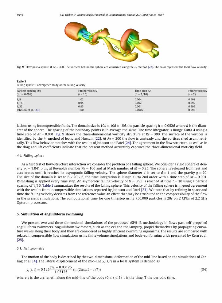
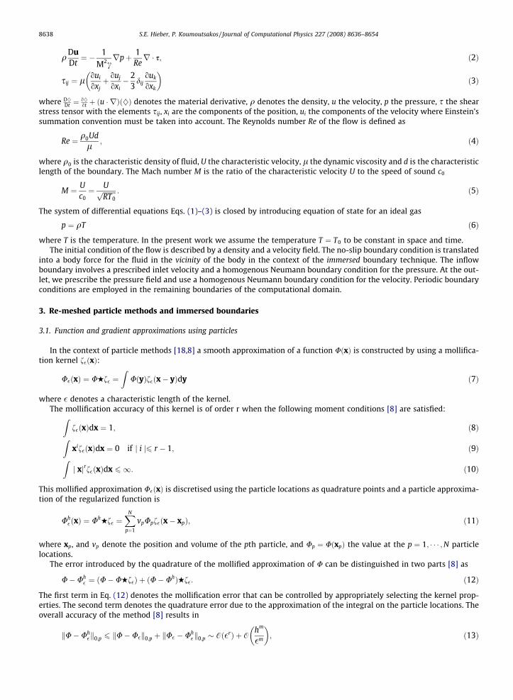
Fig. 9. Flow past a sphere at Re ¼ 300. The vortices behind the sphere are visualized using the k2 method [22]. The color represent the local flow velocity.

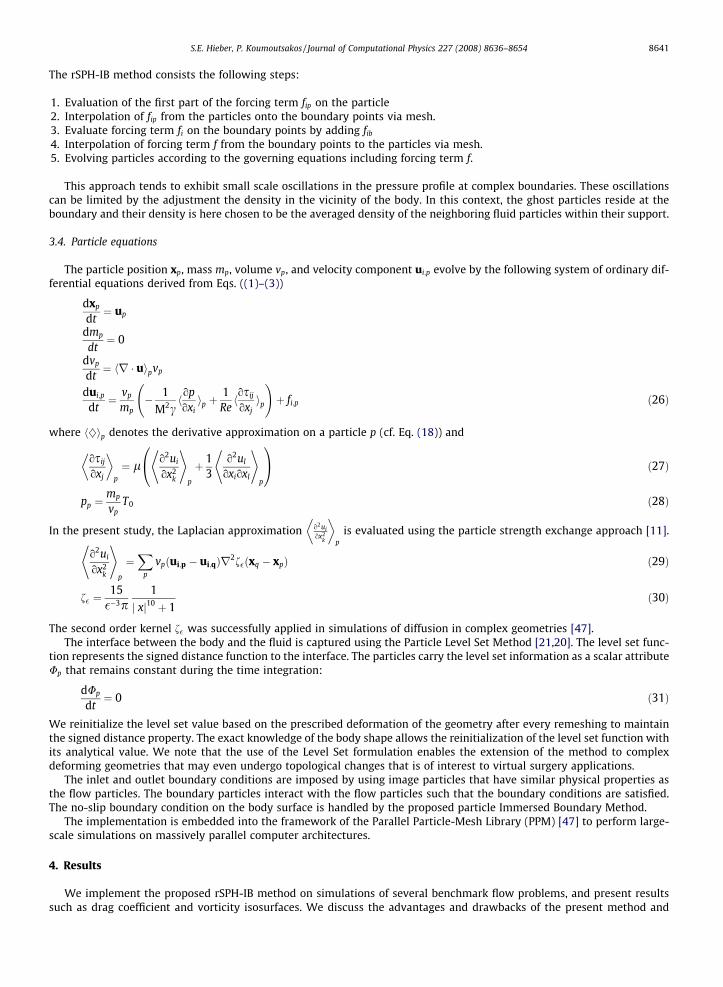
Table 3Falling sphere: Convergence study of the falling velocity

Particle spacing (h) Falling velocity Time step Dt Falling velocity(Dt ¼ 0:001) (t = 10) (h ¼ 1=16) (t = 2)

1/8 1.02 0.004 0.6021/16 0.95 0.002 0.5921/32 0.93 0.001 0.596Johnson et al. [23] 1.00 0.0005 0.595


lations using incompressible fluids. The domain size is 10d� 10d� 15d, the particle spacing h ¼ 0:052d where d is the diam-eter of the sphere. The spacing of the boundary points is in average the same. The time integrator is Runge Kutta 4 using atime step of Dt ¼ 0:001. Fig. 9 shows the three-dimensional vorticity structure at Re ¼ 300. The surface of the vortices isidentified by the k2 method of Jeong and Hussain [22]. At Re ¼ 300 the flow is unsteady and the vortices shed asymmetri-cally. This flow behavior matches with the results of Johnson and Patel [24]. The agreement in the flow structure, as well as inthe drag and lift coefficients indicate that the present method accurately captures the three-dimensional vorticity field.

4.4. Falling sphere

As a first test of flow-structure interaction we consider the problem of a falling sphere. We consider a rigid sphere of den-sity qs ¼ 1:041 > q0 at Reynolds number Re ¼ 100 and at Mach number of M ¼ 0:25. The sphere is released from rest andaccelerates until it reaches its asymptotic falling velocity. The sphere diameter d is set to d ¼ 1 and the gravity g ¼ 20.The size of the domain is set to 6� 20� 6, the time integration is Runge Kutta 2nd order with a time step of Dt ¼ 0:001.Remeshing is applied every time step. An asymptotic falling velocity of U ¼ 0:95 is reached at time t ¼ 10 using a particlespacing of 1=16. Table 3 summarizes the results of the falling sphere. This velocity of the falling sphere is in good agreementwith the results from incompressible simulations reported by Johnson and Patel [23]. We note that by refining in space andtime the falling velocity deviates from the reference value an effect that may be attributed to the compressibility of the flowin the present simulations. The computational time for one timestep using 750,000 particles is 28s on 2 CPUs of 2.2 GHzOpteron processors.

5. Simulation of anguilliform swimming

We present two and three-dimensional simulations of the proposed rSPH-IB methodology in flows past self-propelledanguilliform swimmers. Anguilliform swimmers, such as the eel and the lamprey, propel themselves by propagating curva-ture waves along their body and they are considered as highly efficient swimming organisms. The results are compared withrelated incompressible flow simulations using finite volume simulations and body-conforming grids presented by Kern et al.[25].

5.1. Fish geometry

The motion of the body is described by the two-dimensional deformation of the mid-line based on the simulations of Car-ling et al. [4]. The lateral displacement of the mid-line ysðs; tÞ in a local system is defined as

ysðs; tÞ ¼ 0:125s=Lþ 0:03125

1:03125sinð2pðs=L� t=TÞÞ ð34Þ

where s is the arc length along the mid-line of the body (0 6 s 6 L), t is the time, T the periodic time.


The three dimensional body of the swimmer is described by spatially varying ellipsoid cross sections. The length of thetwo half axis wðsÞ and hðsÞ are defined as

Fig. 10.respect

Fig. 11.gray, re

wðsÞ ¼

ffiffiffiffiffiffiffiffiffiffiffiffiffiffiffiffiffiffiffiffiffi2whs� s2

p0 6 s 6 sb

wh � ðwh �wtÞ s�sbst�sb

� �2sb 6 s 6 st

wtL�sL�st

st 6 s 6 L

8>>><>>>:

ð35Þ

hðsÞ ¼ b

ffiffiffiffiffiffiffiffiffiffiffiffiffiffiffiffiffiffiffiffiffiffiffiffiffiffiffi1� s� a

a

� �2r

ð36Þ

where wh ¼ sb ¼ 0:04L, st ¼ 0:95L, wt ¼ 0:01L, a ¼ 0:51L and b ¼ 0:08L. We apply a no-slip boundary condition on the surfaceof the body. The mid-line of the body is embedded into a non-inertial ðx0; y0Þ-system where the center of mass of the deform-ing body remains and the total angular momentum is conserved. The fluid-body interactions are computed in the inertialsystem (x,y,z) considering the swimmer as a rigid body. Thus, the motion of the body in the global system ðO; x; y; zÞ is de-scribed by the Newtons equations of motion:

0 2 4 6 8−0.2

0

0.2

0.4

0.6

t

U, V

Longitudinal (solid line) and lateral velocity (dashed line) of the two dimensional swimmer compared to finite volume solution (light blue or gray,ively) [25]. (For interpretation of the references to colour in this figure legend, the reader is referred to the web version of this article.)

0 2 4 6 8

−0.1

−0.05

0

0.05

t

C||

0 2 4 6 8

−0.2

0

0.2

t

C⊥

0 2 4 6 8−0.05

0

0.05

t

CM

Longitudinal force Ck , lateral force C? and torque CM of the two dimensional swimmer (black) compared to finite volume solution (light blue orspectively) [25]. (For interpretation of the references to colour in this figure legend, the reader is referred to the web version of this article.)

Fig. 12.t + 0.25


m€xc ¼ F; ð37Þ_Iz _uc þ Iz €uc ¼ Mz; ð38Þ

where m is the total mass of the immersed body, xc represents the position of the center of mass, uc the global angle withrespect to the initial position, F and Mz are the fluid force and yaw torque acting on the body surface. The time-dependency ofthe inertial moment _Iz about the yaw axis is also considered although it is small compared to the inertial moment itself.

We set the viscosity of the fluid to be l ¼ 1:4� 10�4, the body length L ¼ 1, the density q0;fluid ¼ qbody ¼ q ¼ 1 resulting ina Reynolds number of 3850 based on the final swimming speed.

The fluid forces acting on the body are shown as non-dimensional coefficients Ck ¼ Fk=ð0:5qU20SÞ and C? ¼ F?=ð0:5qU2

0SÞparallel and lateral to the swimming direction, where S represents the circumference in two-dimensions and the surface ofthe body in three dimensions. The yaw torque is measured in the non-dimensional coefficient CM ¼ Mz=ð0:5qU2

0LSÞ.

5.2. Equations of motion for the anguilliform swimmer

The position xc and the angle uc of anguilliform swimmer evolve by the following set of equations based on Eqs. (37) and(38)

dxc

dt¼ uc;

duc

dt¼ F

m;

duc

dt¼ xc; ð39Þ

dxc

dt¼ Mz � _Izxc

Iz;

where uc denotes the velocity of the swimmer and xc the angular velocity. We solve this set of equations simultaneouslywith the particle equations Eqs. ((26)–(31)) that describe the fluid behavior.

Vorticity field of the two-dimensional swimmer using rSPH-IB (left) and reference solution of Kern [25] (right) for one swimming cycle at time t,T, t + 0.5T, and t + 0.75T.


5.3. Computational setup

We integrate the Eqs. (26)–(31), and (39) with respect to time using a explicit 4th order Runge-Kutta scheme with timestep of Dt ¼ 0:001. The particles are distributed uniformly in the domain and remeshed every time step. We consider thedomain as an noninertial coordinate system that moves with the opposite x1-component of the fish velocity such that x1-position of the fish is constant in the noninertial coordinate system. Thus, we accelerate the fluid in x1-direction by the oppo-site force that acts on the swimmer and the swimmer remains on its x1-position. The size of the domain is 4� 2 in twodimensions and 3� 2� 2 in three dimensions. This domain size is tested to be sufficiently large to make negligible the influ-ence of the boundary. The simulations are based on 1:3� 105 particles in two dimensions, and 25� 106 particles in threedimensions.

Fig. 13. Zoom of the vorticity field at the tail of the two-dimensional swimmer using rSPH-IB (left) and reference solution of Kern [25] (right) for oneswimming cycle at time t, t + 0.25T, t + 0.5T, and t + 0.75T.


5.4. Results

5.4.1. Two-dimensional anguilliform swimmerWe present a comparison in the two dimensional flows with the work of Kern et al. [25] in terms of the swimming

velocity, as well as forces and torque acting on the swimmer. The swimmer accelerates from rest to an asymptoticmean forward velocity of Uk ¼ 0:54 in about seven undulation cycles. The velocity varies slightly during a cycle whilethe lateral velocity U? has an amplitude of 0.04. The time history of the longitudinal and lateral velocity agrees verywell with the incompressible solution (Fig. 10). The velocity differs the most at time 1 < t < 4 where the density vari-ations are larger than at later time steps. The higher density variations lead to higher pressure variations resulting inlarger forces acting on the swimmer. The incompressible solution is approximated sufficiently with a Mach number ofM ¼ 0:1.

The longitudinal and lateral forces and the torque (Fig. 11) agree very well with the incompressible solution. The forceand moment coefficient Ck;C? and CM converge to oscillation modes with zero mean and a constant amplitude of 0.03,0.04 and 0.03, respectively. After the body has accelerated to its mean swimming velocity the forces acting on the body havea zero mean. The computation of one time step took 10s on 8 processors for 800,000 particles.

0 2 4 6 8

−0.1

−0.05

0

0.05

t

C||

0 2 4 6 8

−0.2

0

0.2

t

C⊥

0 2 4 6 8−0.05

0

0.05

t

CM

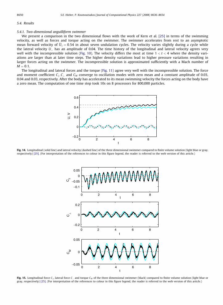
Fig. 15. Longitudinal force Ck , lateral force C? and torque CM of the three dimensional swimmer (black) compared to finite volume solution (light blue orgray, respectively) [25]. (For interpretation of the references to colour in this figure legend, the reader is referred to the web version of this article.)

0 2 4 6 8−0.2

0

0.2

0.4

0.6

t

U, V

Fig. 14. Longitudinal (solid line) and lateral velocity (dashed line) of the three dimensional swimmer compared to finite volume solution (light blue or gray,respectively) [25]. (For interpretation of the references to colour in this figure legend, the reader is referred to the web version of this article.)


The compressibility of the fluid causes unresolved pressure waves resulting in high frequent noise in the flow structure. Asecond order filter [43] is applied to the mass and the momentum during the remeshing process every 100 steps to suppressthe small scale pressure waves in the range of the Nyquist frequency. We note that Kern et al. [25] applied a low pass filter tothe fluid force F and the torque Mz in order to stabilize the simulation of the incompressible flow. In the present method theflow-structure is stable and we can omit the use of such a low pass filter.

Figs. 12 and 13 show the vorticity field of the swimmer during one period at the final swimming speed along with a zoomat the tail. The main differences in the vorticity field result from the fact that the particle solution is uniformly resolved,whereas the finite volume solution involves an adaptive re-gridding. Thus, the vorticity shedding at the boundary layer isbetter resolved in the finite volume solution.

The tail beat amplitude is A ¼ 0:16 and the corresponding Strouhal number is St ¼ 0:59. The wave velocity is V ¼ 0:73,which results in a slip of Uk=V ¼ 0:74.

5.4.2. Three-dimensional anguilliform swimmerIn three dimensions the forces acting on the fish compare well with the finite volume solution (Fig. 15). The net force and

moment coefficient Ck;C? and CM oscillate with a mean of zero and amplitudes of 0.04, 0.06 and 0.03, respectively. Fig. 14shows that the final swimming speed in the particle solution (uSPH ¼ 0:448) is 12% higher than the velocity reported in thefinite volume solution (uFV ¼ 0:402). This result is consistent with the drag values reported in the flow past a sphereat Re ¼ 300 that were found to differ approximately 10% from the results of grid based methods (Table 2). The forwardvelocity Uk oscillates with an amplitude of 0.01. The lateral velocity U? has a zero mean and an amplitude of 0.03(Fig. 14). The wave velocity V ¼ 0:73 is equal to the two dimensional case resulting in the slip of Uk=V ¼ 0:61. The tail beatamplitude is determined to be A ¼ 0:15 with St ¼ 0:67.

The oscillating tail of the swimmer sheds vortex rings in the wake with the frequency of the swimming motion (Figs. 16–18). Both, the particle and the finite volume solution show the vorticity shed in every half tail beat cycle that breaks up intotwo vortices resulting in near wake lateral jets. The vorticity field of particle solution appears smoother and shows lesssmall-scale structures. The vortex rings are less recognizable. As the finite-volume grid feature a four times higher resolution

Fig. 16. Vorticity field of the three-dimensional swimmer using rSPH-IB (left) and reference solution of Kern [25] (right) for one swimming cycle at time t,t + 0.25T, t + 0.5T, and t + 0.75T.

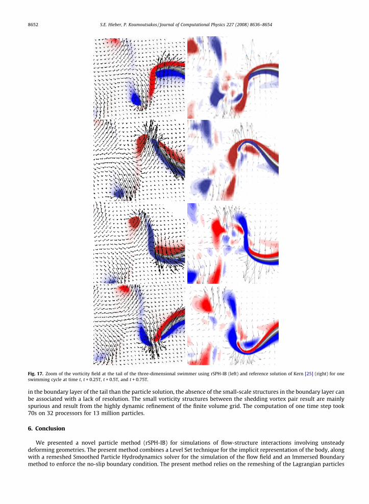
Fig. 17. Zoom of the vorticity field at the tail of the three-dimensional swimmer using rSPH-IB (left) and reference solution of Kern [25] (right) for oneswimming cycle at time t, t + 0.25T, t + 0.5T, and t + 0.75T.


in the boundary layer of the tail than the particle solution, the absence of the small-scale structures in the boundary layer canbe associated with a lack of resolution. The small vorticity structures between the shedding vortex pair result are mainlyspurious and result from the highly dynamic refinement of the finite volume grid. The computation of one time step took70s on 32 processors for 13 million particles.

6. Conclusion

We presented a novel particle method (rSPH-IB) for simulations of flow-structure interactions involving unsteadydeforming geometries. The present method combines a Level Set technique for the implicit representation of the body, alongwith a remeshed Smoothed Particle Hydrodynamics solver for the simulation of the flow field and an Immersed Boundarymethod to enforce the no-slip boundary condition. The present method relies on the remeshing of the Lagrangian particles

Fig. 18. Isosurface of the vorticity magnitude (left) and vortices visualized by the k2-method (right) of the three-dimensional swimmer using rSPH-IB forone swimming cycle at time t, t + 0.25T, t + 0.5T, and t + 0.75T.


on a rectangular grid. This remeshing does not detract from the adaptive character of the method as the particles adapt toresolve the flow field and at the same time it ensures the convergence of the method when the particles get distorted by theflow map. The efficiency and accuracy of the method, as well as comparison with related methodologies, is demonstrated in anumber of two and three dimensional benchmark problems and the method is shown to be well capable in solving problemsof fluid-structure interaction. The simplicity of the method in handling complex boundaries makes it suitable for large scalesimulations, employing millions of particles for the simulation of complex movement of flexible structures as they appear forexample in anguilliform swimming. A drawback of the present method is the need to account for the compressibility of theflow. Fast motions of the boundary in high Reynolds number flows result in pressure waves in the fluid that restrict the timestep and can lead to numerical problems when not properly resolved. The use of artificial damping terms may help to rem-edy the situation much as it is the case in artificial compressibility methods. Another limitation of the present rSPH-IB for-mulation is the use of a uniform particle size throughout the computational domain. We are currently addressing thisinefficiency of the method by incorporating multi-resolution particle techniques [2,3] and developing its implementationon GPUs following related work on Vortex Methods [46]. The present method allows for simulations past complex deforminggeometries, while the level set description of the surface enables flow simulations even past bodies that undergo topologicalchanges. We pursue applications of this method to other problems related to swimming and flying in nature, as well as tosimulations of flow-structure interaction as they pertain to virtual surgery.

Acknowledgment

We would like to thank Dr. Stefan Kern (ETHZ) and Prof. Tony Leonard (Caltech) for several helpful discussions through-out this work. We wish to acknowledge several helpful interactions with Caroline Hieber during the writing of this paper.


This project was funded by the Swiss National Science Foundation, NCCR’ Computer Aided and Image Guided Medical Inter-ventions’ (Co-Me).

References

[1] J.T. Beale, A convergent 3-D vortex method with grid-free stretching, Math. Comput. 46 (1986) 401–424.[2] M. Bergdorf, G.-H. Cottet, P. Koumoutsakos, Multilevel adaptive particle methods for convection-diffusion equations, Multiscale Model. Simul. 4 (1)

(2005) 328–357.[3] M. Bergdorf, P. Koumoutsakos, A lagrangian particle-wavelet method, Multiscale Model. Simul. 14 (2006) 980–995.[4] John Carling, Thelma L. Williams, Graham Bowtell, Self-propelled anguilliform swimming: simultaneous solution of the two-dimensional Navier–

Stokes equations and Newtons’ laws of motion, J. Exp. Biol. 201 (1998) 3143–3166.[5] A.K. Chaniotis, D. Poulikakos, P. Koumoutsakos, Remeshed smoothed particle hydrodynamics for the simulation of viscous and heat conducting flows, J.

Comput. Phys. 182 (1) (2002) 67–90.[6] A.J. Chorin, Numerical study of slightly viscous flow, J. Fluid Mech. 57 (4) (1973) 785–796.[7] G.-H. Cottet, Artificial viscosity models for vortex and particle methods, J. Comput. Phys. 127 (1996) 299–308.[8] G.-H. Cottet, P. Koumoutsakos, Vortex Methods – Theory and Practice, Cambridge University Press, New York, 2000.[9] Georges-Henri Cottet, Bertrand Michaux, Sepand Ossia, Geoffroy VanderLinden, A comparison of spectral and vortex methods in three-dimensional

incompressible flows, J. Comput. Phys. 175 (2002) 702–712.[10] G.H. Cottet, E. Maitre, A level set method for fluid-structure interactions with immersed surfaces, Mathematical Models and Methods in the Applied

Sciences 16 (2006) 415–438.[11] P. Degond, S. Mas-Gallic, The weighted particle method for convection-diffusion equations. Part 1: The case of an isotropic viscosity, Math. Comput. 53

(188) (1989) 485–507.[12] A. Dupuis, P. Chatelain, P. Koumoutsakos, An immersed boundary-lattice boltzmann method for the simulation of the flow past an impulsively started

cylinder, J. Comput. Phys. 227 (9) (2008) 4486–4498.[13] Jeff D. Eldredge, Anthony Leonard, Tim Colonius, A general determistic treatment of derivatives in particle methods, J. Comput. Phys. 180 (2) (2002)

686–709.[14] E.A. Fadlun, R. Verzicco, P. Orlandi, J. Mohd-Yusof, Combined immersed-boundary finite-difference methods for three-dimensional complex flow

simulations, J. Comput. Phys. 161 (1) (2000) 35–60.[15] C. Farhat, M. Lesoinne, Automatic partitioning of unstructured meshes for the parallel solution of problems in computational mechanics, Int. J. Numer.

Methods Eng. 36 (5) (1993) 745.[16] Bengt Fornberg, Steady viscous flow past a sphere at high Reynolds numbers, J. Fluid Mech. 190 (1988) 471–489.[17] R.A. Gingold, J.J. Monaghan, Smoothed particle hydrodynamics: theory and application to non-spherical stars, Month Notices Roy. Astron. Soc. 181

(1977) 375–389.[18] Ole H. Hald, Convergence of vortex methods for Euler’s equations, III, SIAM J. Numer. Anal. 24 (3) (1987) 538–582.[19] R.D. Henderson, Details of the drag curve near the onset of vortex shedding, Phys. Fluids 7 (1995) 2102–2104.[20] S.E. Hieber, J.H. Walther, P. Koumoutsakos, Remeshed smoothed particle hydrodynamics simulation of the mechanical behavior of human organs, J.

Technol. Health Care 12 (4) (2004) 305–314.[21] Simone Elke Hieber, Petros Koumoutsakos, A Lagrangian particle level set method, J. Comput. Phys. 210 (2005) 342–367.[22] H. Jeong, B. Tombor, R. Albert, Z.N. Oltvai, A.-L. Barabási, The large-scale organization of metabolic networks, Nature 407 (2000) 651–654.[23] A.T. Johnson, V.C. Patel, Flow past a sphere up to a Reynolds number of 300, J. Fluid Mech. 378 (1999) 19–70.[24] Gordon R. Johnson, Robert A. Stryk, Stephen R. Beissel, SPH for high velocity impact computations, Comput. Meth. Appl. Mech. Eng. 139 (1996) 347–

373.[25] Stefan Kern, Petros Koumoutsakos, Simulations of optimized anguilliform swimming, J. Exp. Biol. 209 (2006) 4841–4857.[26] Jungwoo Kim, Dongjoo Kim, Haecheon Choi, An immersed-boundary finite-volume method for simulations of flow in complex geometries, J. Comput.

Phys. 171 (2001) 132–150.[27] P. Koumoutsakos, Inviscid axisymmetrization of an elliptical vortex ring, J. Comput. Phys. 138 (1997) 821–857.[28] P. Koumoutsakos, Vorticity flux control in a turbulent channel flow, Phys. Fluids 11 (2) (1999) 248–250.[29] P. Koumoutsakos, Multiscale flow simulations using particles, Annu. Rev. Fluid Mech. 37 (2005) 457–487.[30] P. Koumoutsakos, A. Leonard, High-resolution simulation of the flow around an impulsively started cylinder using vortex methods, J. Fluid Mech. 296

(1995) 1–38.[31] A. Leonard, Review. vortex methods for flow simulation, J. Comput. Phys. 37 (1980) 289–335.[32] A.L.F. Lima E Silva, A. Silveira-Neto, J.J.R. Damasceno, Numerical simulations of two-dimensional flows over a circular cylinder using the immersed

boundary method, J. Comput. Phys. 189 (2003) 351–370.[33] L.B. Lucy, A numerical approach to the testing of the fission hypothesis, Astron. J. 82 (1977) 1013–1024.[34] Rajat Mittal, Gianluca Iaccarino, Immersed boundary methods, Annu. Rev. Fluid Mech. 37 (2005) 239–261.[35] J.J. Monaghan, Smoothed particle hydrodynamics, Annu. Rev. Astron. Astrophys. 30 (1992) 543–574.[36] J.J. Monaghan, Smoothed particle hydrodynamics, Rep. Progress Phys. 68 (8) (2005) 1703–1759.[37] G. Morgenthal, J.H. Walther, An immersed interface method for the vortex-in-cell algorithm, Comput. Struct. 85 (2007) 712–726.[38] J. Park, K. Kwon, H. Choi, Numerical solutions of flow past a cylinder at Reynolds number up to 160, KSME Int. J. 12 (6) (1998) 1200–1205.[39] Charles Peskin, Flow patterns around heart valves: A numerical study, J. Comput. Phys. 10 (1972) 252–271.[40] C.S. Peskin, Numerical analysis of blood flow in the heart, J. Comput. Phys. 25 (1977) 220–252.[41] C.S. Peskin, The immersed boundary method, Acta Numer. 11 (2002) 479–517.[42] C.S. Peskin, D.M. McQueen, Modeling prosthetic heart-valves for numerical analysis of blood flow in the heart, J. Comput. Phys. 37 (1980) 113–132.[43] Roger Peyret, Thomas Taylor, Computational Methods for Fluid Flow, Springer-Verlag, 1983.[44] P. Ploumhans, G.S. Winckelmans, J.K. Salmon, A. Leonard, M.S. Warren, Vortex methods for direct numerical simulation of three-dimensional bluff

body flows: Applications to the sphere at Re ¼ 300, 500 and 1000, J. Comput. Phys. 178 (2002) 427–463.[45] Anatol Roshko, Experiments on the flow past a circular cylinder at very high Reynolds number, J. Fluid Mech. 10 (3) (1961) 345–356.[46] Diego Rossinelli, Petros Koumoutsakos, Vortex methods for incompressible flow simulations on the GPU, Visual Comput. 12 (2008).[47] I.F. Sbalzarini, J.H. Walther, M. Bergdorf, S.E. Hieber, E.M. Kotsalis, P. Koumoutsakos, PPM – a highly efficient parallel particle-mesh library for the

simulation of continuum systems, J. Comput. Phys. 215 (2006) 566–588.[48] S.P. Singh, S. Mittal, Flow past a cylinder: shear layer instability and drag crisis, Int. J. Numer. Methods Fluids 47 (2005) 75–98.[49] Xiaodong Wang, Wing Kam Liu, Extended immersed boundary method using fem and rkpm, Comput. Methods Appl. Mech. Eng. 193 (12–14) (2004)

1305–1321.[50] C.H.K. Williamson, Oblique and parallel modes of vortex shedding in the wake of a circular cylinder at low Reynolds numbers, J. Fluid Mech. 206 (1989)

579–627.

1-s2.0-S0021999108003343-main

Documents

Transcript of 1-s2.0-S0021999108003343-main