1 Reasoning in Uncertain Situations 8 8.0Introduction 8.1Logic-Based Abductive Inference...
90
1 Reasoning in Uncertain Situations 8 8.0 Introduction 8.1 Logic-Based Abductive Inference 8.2 Abduction: Alternatives to Logic 8.3 The Stochastic Approach to Uncertainty 8.4 Epilogue and References 8.5 Exercises
-
Upload
martina-lamb -
Category
Documents
-
view
218 -
download
4
Transcript of 1 Reasoning in Uncertain Situations 8 8.0Introduction 8.1Logic-Based Abductive Inference...

1
Reasoning in Uncertain Situations 8 8.0 Introduction
8.1 Logic-Based AbductiveInference
8.2 Abduction: Alternativesto Logic
8.3 The Stochastic Approach to Uncertainty
8.4 Epilogue and References
8.5 Exercises
2
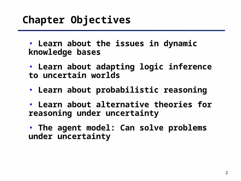
Chapter Objectives
• Learn about the issues in dynamic knowledge bases
• Learn about adapting logic inference to uncertain worlds
• Learn about probabilistic reasoning
• Learn about alternative theories for reasoning under uncertainty
• The agent model: Can solve problems under uncertainty

3
Uncertain agent
environmentagent
?
sensors
actuators
??
??
?
model

4
Types of Uncertainty
• Uncertainty in prior knowledge
E.g., some causes of a disease are unknown and are not represented in the background knowledge of a medical-assistant agent

5
Types of Uncertainty
• Uncertainty in actions
E.g., to deliver this lecture: I must be able to come to school the heating system must be working my computer must be working the LCD projector must be working I must not have become paralytic or blind
As we discussed last time, actions are represented with relatively short lists of preconditions, while these lists are in fact arbitrary long. It is not efficient (or even possible) to list all the possibilities.

6
Types of Uncertainty
• Uncertainty in perception
E.g., sensors do not return exact or complete information about the world; a robot never knows exactly its position.
Courtesy R. Chatila
7
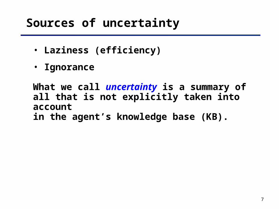
Sources of uncertainty
• Laziness (efficiency)
• Ignorance
What we call uncertainty is a summary of all that is not explicitly taken into account in the agent’s knowledge base (KB).

8
Assumptions of reasoning with predicate logic (1)
(1) Predicate descriptions must be sufficient with respect to the application domain.
Each fact is known to be either true or false. But what does lack of information mean?
Closed world assumption, assumption based reasoning:
PROLOG: if a fact cannot be proven to be true, assume that it is false
HUMAN: if a fact cannot be proven to be false, assume it is true

9
Assumptions of reasoning with predicate logic (2)
(2)The information base must be consistent.
Human reasoning: keep alternative (possibly conflicting) hypotheses. Eliminate as new evidence comes in.

10
Assumptions of reasoning with predicate logic (3)
(3) Known information grows monotonically through the use of inference rules.
Need mechanisms to:
• add information based on assumptions (nonmonotonic reasoning), and
• delete inferences based on these assumptions in case later evidence shows that the assumption was incorrect (truth maintenance).

11
Questions
How to represent uncertainty in knowledge?
How to perform inferences with uncertain knowledge?
Which action to choose under uncertainty?

12
Approaches to handling uncertainty
Default reasoning [Optimistic]non-monotonic logic
Worst-case reasoning [Pessimistic]adversarial search
Probabilistic reasoning [Realist]probability theory
13
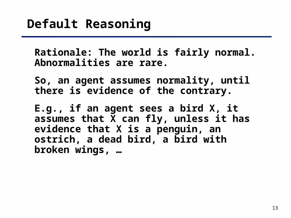
Default Reasoning
Rationale: The world is fairly normal. Abnormalities are rare.
So, an agent assumes normality, until there is evidence of the contrary.
E.g., if an agent sees a bird X, it assumes that X can fly, unless it has evidence that X is a penguin, an ostrich, a dead bird, a bird with broken wings, …

14
Modifying logic to support nonmonotonic inference
p(X) unless q(X) r(X)
If we
• believe p(X) is true, and
• do not believe q(X) is true
then we
• can infer r(X)
“unless” is a modal operator.

15
Modifying logic to support nonmonotonic inference (cont’d)
p(X) unless q(X) r(X) in KB
p(Z) in KB
r(W) s(W) in KB
- - - - - -
q(X) CWA, q(X) is not in KB
r(X) inferred
s(X) inferred

16
Example
If it is snowing and unless there is an exam tomorrow, I can go skiing.
It is snowing.
Whenever I go skiing, I stop by at the Chalet to drink hot chocolate.
- - - - - -
I did not check my calendar but I don’t remember an exam scheduled for tomorrow, conclude: I’ll go skiing. Then conclude: I’ll drink hot chocolate.

17
“Abnormality”
p(X) unless ab p(X) q(X)
ab: abnormal
Examples: If X is a bird, it will fly unless it isabnormal.
(abnormal: broken wing, sick, trapped, ostrich, ...)
If X is a car, it will run unless it isabnormal.
(abnormal: flat tire, broken engine, no gas, …)

18
Another modal operator: M
p(X) M q(X) r(X)
If
• we believe p(X) is true, and
• q(X) is consistent with everything else,
then we
• can infer r(X)
“M” is a modal operator for “is consistent.”

19
Example
X good_student(X) M study_hard(X) graduates (X)
How to make sure that study_hard(X) is consistent?
Negation as failure proof: Try to prove study_hard(X), if not possible assume X does study.
Tried but failed proof: Try to prove study_hard(X ), but use a heuristic or a time/memory limit. When the limit expires, if no evidence to the contrary is found, declare as proven.

20
Potentially conflicting results
X good_student(X) M study_hard(X) graduates (X)
X good_student(X) M study_hard(X) graduates (X)
good_student(peter)
party_person(peter)
If the KB does not contain information about study_hard(peter), both graduates(peter) and graduates (peter) will be inferred!
Solutions: autoepistemic logic, default logic, inheritance search, ...

21
Truth Maintenance Systems
They are also known as reason maintenance systems, or justification networks.
In essence, they are dependency graphs where rounded rectangles denote predicates, and half circles represent facts or “and”s of facts.
Base (given) facts: ANDed facts:
p is in the KB p q r
p r
p
q

22
Example
When p, q, s, x, and y are given, all of r, t, z, and u can be inferred.
r
p
q
s
x
y
z
t
u

23
Example (cont’d)
If p is retracted, both r and u must be retracted. (Compare this to chronological backtracking.)
r
p
q
s
x
y
z
t
u

24
Example (cont’d)
If x is retracted (in the case before the previous slide), z must be retracted.
r
p
q
s
x
y
z
t
u
25
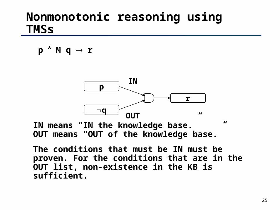
Nonmonotonic reasoning using TMSs
p M q r
IN means “IN the knowledge base.” OUT means “OUT of the knowledge base.”
The conditions that must be IN must be proven. For the conditions that are in the OUT list, non-existence in the KB is sufficient.
r
p
q
IN
OUT
26
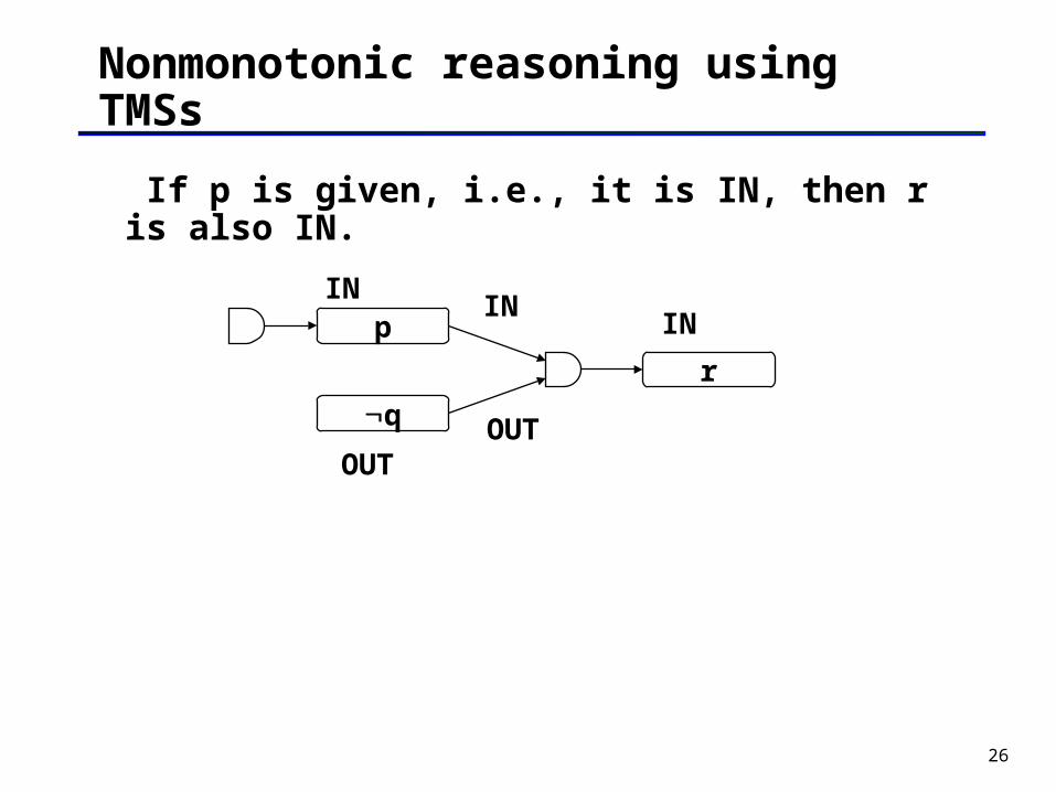
Nonmonotonic reasoning using TMSs
If p is given, i.e., it is IN, then r is also IN.
r
p
q
IN
OUT
ININ
OUT

27
Nonmonotonic reasoning using TMSs
If q is now given, r must be retracted, it becomes OUT. Note that when q is given the knowledge base contains more facts, but the set of inferences shrinks (hence the name nonmonotonic reasoning.)
r
p
q
IN
IN
INOUT
OUT

28
A justification network to believe that Pat studies hard
X good_student(X) M study_hard(X) study_hard (X)
good_student(pat)
good_student(pat)IN
OUT
ININ
OUTstudy_hard(pat)
study_hard(pat)

29
It is still justifiable that Pat studies hard
X good_student(X) M study_hard(X) study_hard (X)
Y party_person(Y) study_hard (Y)
good_student(pat)
good_student(pat)IN
OUT
ININ
OUTstudy_hard(pat)
study_hard(pat)
party_person(pat)
OUT
IN

30
“Pat studies hard” is no more justifiable
X good_student(X) M study_hard(X) study_hard (X)
Y party_person(Y) study_hard (Y)
good_student(pat)
party_person(pat)
good_student(pat)IN
OUT
ININ
OUTstudy_hard(pat)
study_hard(pat)
party_person(pat)
OUT
IN
IN
IN
OUT
31
Notes
We looked at JTMSs (Justification Based Truth Maintenance Systems). “Predicate” nodes in JTMSs are pure text, there is even no information about “”. With LTMSs (Logic Based Truth Maintenance Systems), “” has the same semantics as logic. So what we covered was technically LTMSs.
We will not cover ATMSs (Assumption Based Truth Maintenance Systems).
Did you know that TMSs were first developed for Intelligent Tutoring Systems (ITS)?
32
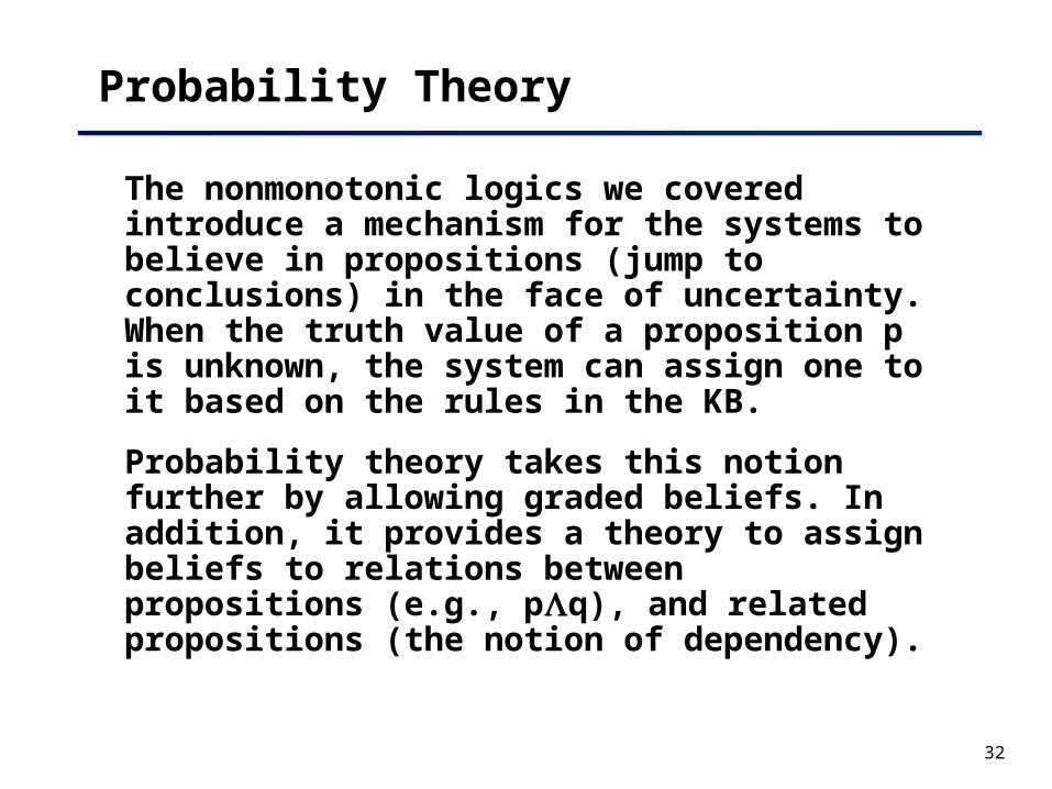
Probability Theory
The nonmonotonic logics we covered introduce a mechanism for the systems to believe in propositions (jump to conclusions) in the face of uncertainty. When the truth value of a proposition p is unknown, the system can assign one to it based on the rules in the KB.
Probability theory takes this notion further by allowing graded beliefs. In addition, it provides a theory to assign beliefs to relations between propositions (e.g., pq), and related propositions (the notion of dependency).

33
Probabilities for propositions
We write probability(A), or frequently P(A) in short, to mean the “probability of A.”
But what does P(A) mean?
P(I will draw ace of hearts)
P(the coin will come up heads)
P(it will snow tomorrow)
P(the sun will rise tomorrow)
P(the problem is in the third cylinder)
P(the patient has measles)
34
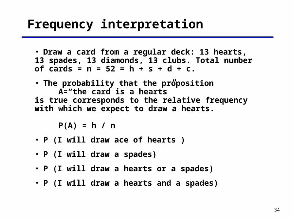
Frequency interpretation
• Draw a card from a regular deck: 13 hearts, 13 spades, 13 diamonds, 13 clubs. Total number of cards = n = 52 = h + s + d + c.
• The probability that the proposition A=“the card is a hearts”
is true corresponds to the relative frequency with which we expect to draw a hearts.
P(A) = h / n
• P (I will draw ace of hearts )
• P (I will draw a spades)
• P (I will draw a hearts or a spades)
• P (I will draw a hearts and a spades)

35
Subjective interpretation
• There are many situations in which there is no objective frequency interpretation:
On a cold day, just before letting myself glide from the top of Mont Ripley, I say “there is probability 0.2 that I am going to have a broken leg”.
You are working hard on your AI class and you believe that the probability that you will get an A is 0.9.
• The probability that proposition A is true corresponds to the degree of subjective belief.

36
Axioms of probability
• There is a debate about which interpretation to adopt . But there is general agreement about the underlying mathematics.
• Values for probabilities should satisfy the following requirements:
The probability of a proposition A is a real number P(A) between 0 and 1: 0 P(A) 1.
The probability of “always true” is 1: P(true) = 1.
If A and B are disjoint, i.e., (A B) then: P(A B) = P(A) + P(B).

37
These axioms are all that is needed
• From them, one can derive all there is to say about probabilities.
• For example we can show that: P(A) = 1 - P(A) because
P(A A) = P (true) by logic P(A A) = P(A) + P(A) by the third axiom
P(true) = 1 by the second axiomP(A) + P(A) = 1 combine the above
P(false) = 0 because
false = true by logicP(false) = 1 - P(true) by the above
P(A B) = P(A) + P(B) - P(A B) because intersection area is counted twice.

38
Random variables
• The events we are interested in have a set of possible values. These values are mutually exclusive, and exhaustive.
• For example: coin toss: {heads, tails} roll a die: {1, 2, 3, 4, 5, 6} weather: {snow, sunny, rain, fog} measles: {true, false}
• For each event, we introduce a random variable which takes on values from the associated set. Then we have: P(C = tails) rather than P(tails) P(D = 1) rather than P(1) P(W = sunny) rather than P(sunny) P(M = true) rather than P(measles)

39
Probability Distribution
A probability distribution is a listing of probabilities for every possible value a single random variable might take.
For example:
1/6
1/6
1/6
1/6
1/6
1/6
weather
snow
rain
fog
sunny
prob.
0.2
0.1
0.1
0.6

40
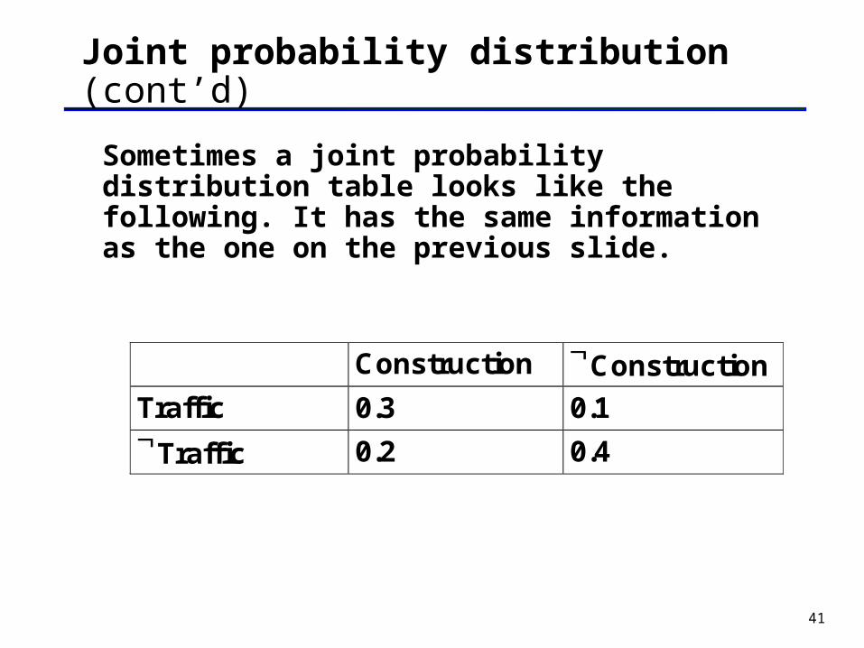
Joint probability distribution
A joint probability distribution for n random variables is a listing of probabilities for all possible combinations of the random variables.
For example:
Construction Traffic ProbabilityTrue True 0.3
True False 0.2
False True 0.1
False False 0.4
41
Joint probability distribution (cont’d)
Sometimes a joint probability distribution table looks like the following. It has the same information as the one on the previous slide.
Construction Construction
Traffic 0.3 0.1Traffic 0.2 0.4

42
Why do we need the joint probability table?
It is similar to a truth table, however, unlike in logic, it is usually not possible to derive the probability of the conjunction from the individual probabilities.
This is because the individual events interact in unknown ways. For instance, imagine that the probability of construction (C) is 0.7 in summer in Houghton, and the probability of bad traffic (T) is 0.05. If the “construction” that we are referring to in on the bridge, then a reasonable value for P(C T) is 0.6. If the “construction” we are referring to is on the sidewalk of a side street, then a reasonable value for P(C T) is 0.04.

43
Dynamic probabilistic KBs
Imagine an event A. When we know nothing else, we refer to the probability of A in the usual way: P(A).
If we gather additional information, say B, the probability of A might change. This is referred to as the probability of A given B: P(A | B).
For instance, the “general” probability of bad traffic is P(T). If your friend comes over and tells you that construction has started, then the probability of bad traffic given construction is P(T | C).
44
Prior probability
The prior probability; often called the unconditional probability, of an event is the probability assigned to an event in the absence of knowledge supporting its occurrence and absence, that is, the probability of the event prior to any evidence. The prior probability of an event is symbolized: P (event).

45
Posterior probability
The posterior (after the fact) probability, often called the conditional probability, of an event is the probability of an event given some evidence. Posterior probability is symbolized P(event | evidence).
What are the values for the following?
P( heads | heads)
P( ace of spades | ace of spades)
P(traffic | construction)
P(construction | traffic)
46
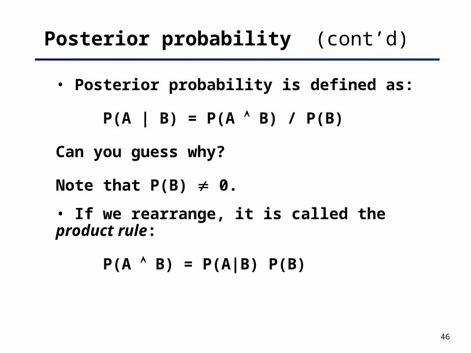
Posterior probability (cont’d)
• Posterior probability is defined as:
P(A | B) = P(A B) / P(B)
Can you guess why?
Note that P(B) 0.
• If we rearrange, it is called the product rule:
P(A B) = P(A|B) P(B)

47
Comments on posterior probability
• P(A|B) can be thought of as:
Among all the occurrences of B, in what proportion do A and B hold together?
• If all we know is P(A), we can use this to compute the probability of A, but once we learn B, it does not make sense to use P(A) any longer.

48
Marginal probabilities
What is the probability of traffic, P(traffic)?
P(traffic) = P(traffic construction) +P(traffic construction)
= 0.3 + 0.1= 0.4
Note that the table should be consistent with respect to the axioms of probability: the values in the whole table should add up to 1; for any event A, P(A) should be 1 - P(A); and so on.
Construction Construction
Traffic 0.3 0.1Traffic 0.2 0.4
0.5
0.6
0.4
0.5 1.0

More on computing probabilities
• P(traffic construction) = 0.3 + 0.1 + 0.2 = 0.6
• P(traffic | construction) = P(traffic construction) / P(construction) = 0.3 / 0.5 = 0.6
• P( construction traffic) = P ( construction traffic) by logic = 0.1 + 0.4 + 0.3 = 0.8
• Compare the previous two cases: the conditional probability is usually not equal to the probability of the conditional!
Construction Construction
Traffic 0.3 0.1Traffic 0.2 0.4
0.5
0.6
0.4
0.5 1.0
50
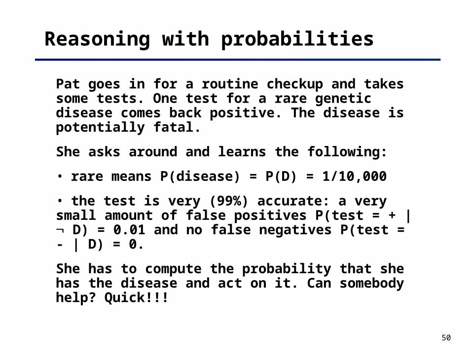
Reasoning with probabilities
Pat goes in for a routine checkup and takes some tests. One test for a rare genetic disease comes back positive. The disease is potentially fatal.
She asks around and learns the following:
• rare means P(disease) = P(D) = 1/10,000
• the test is very (99%) accurate: a very small amount of false positives P(test = + | D) = 0.01 and no false negatives P(test = - | D) = 0.
She has to compute the probability that she has the disease and act on it. Can somebody help? Quick!!!

51
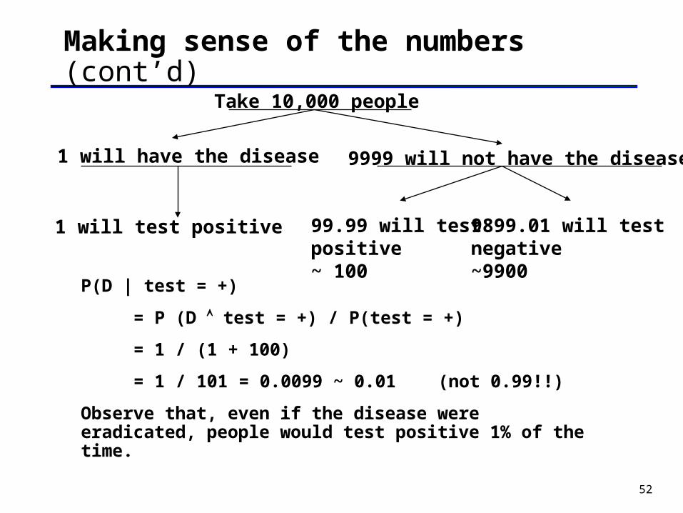
Making sense of the numbers
P(D) = 1/10,000
P(test = + | D) = 0.01, P(test = - | D) = 0.99
P(test = - | D) = 0, P(test = + | D) = 1.
1 will have the disease 9999 will not have the disease
1 will test positive 99.99 will test positive
9899.01 will test negative
Take 10,000 people
52
Making sense of the numbers (cont’d)
P(D | test = +)
= P (D test = +) / P(test = +)
= 1 / (1 + 100)
= 1 / 101 = 0.0099 ~ 0.01 (not 0.99!!)
Observe that, even if the disease were eradicated, people would test positive 1% of the time.
1 will have the disease 9999 will not have the disease
1 will test positive 99.99 will test positive~ 100
9899.01 will test negative~9900
Take 10,000 people

53
Formalizing the reasoning
• Bayes’ rule:
• Apply to the example: P(D | test= +) = P(test= + | D) P(D) / P(test= +) = 1 * 0.0001 / P(test= +)
P(D | test= +) = P(test= + | D) P( D) / P(test= +) = 0.01 * 0.9999 / P(test= +)
P(D | test=+) + P(D | test= +) = 1, so P(test=+)= 0.0001 + 0.009999 = 0.010099
P (D | test= +) = 0.0001 / 0.010099 = 0.0099.
P(E)H)|P(E P(H)
E)|P(H

54
How to derive the Bayes’ rule
• Recall the product rule:P (H E) = P (H | E) P(E)
• is commutative: P (E H) = P (E | H) P(H)
• the left hand sides are equal, so the right hand sides are too:
P(H | E) P(E) = P (E | H) P(H)
• rearrange:P(H | E) = P (E | H) P(H) / P(E)

55
What did commutativity buy us?
• We can now compute probabilities that we might not have from numbers that are relatively easy to obtain.
• For instance, to compute P(measles | rash), you use P(rash|measles) and P(measles).
• Moreover, you can recompute P(measles| rash) if there is a measles epidemic and the P(measles) increases dramatically. This is more advantageous than storing the value for P(measles | rash).

56
What does Bayes’ rule do?
It formalizes the analysis that we did for computing the probabilities:
test = +
has disease
99% of the has-disease population, i.e., those who are correctly identified as having the disease, is much smaller than 1% of the universe, i.e., those incorrectly tagged as having the disease when they don’t.
universe

57
Generalize to more than one evidence
• Just a piece of notation first: we use P(A,B,C) to mean P(A B C).
• General form of Bayes’ rule:
P(H | E1, E2, … , En) = P(E1, E2, … , En | H) * P(H) / P(H)
• But knowing E1, E2, … , En requires a joint probability table for n variables. You know that this requires 2n values.
• Can we get away with less?

58
Yes.
• Independence of some events result in simpler calculations.Consider calculating P(E1, E2, … , En). If E1, …, Ei-1 are related to weather, and Ei, …, En are related to measles, there must be some way to reason about them separately.
• Recall the coin toss example. We know that subsequent tosses are independent: P( T1 | T2) = P(T1)
From the product rule we have: P(T1 T2 ) = P(T1 | T2) x P(T2) .
This simplifies to P(T1) x P(T2) for P(T1 T2 ) .

59
Formally,
X and Y are said to be conditionally independent, given Z, if is it is true thatP(X | Y,Z) = P(X|Z).
In other words, the presence of Z makes additional information Y irrelevant.

60
Graphically,
Cavity is the common cause of both symptoms. Toothache and cavity are independent, given a catch by a dentist with a probe:
P(catch | cavity, toothache) = P(catch | cavity),P(toothache | cavity, catch) = P(toothache | cavity).
cavity
Tooth-ache
catch
weather

61
Another example
Measles and allergy influence rash independently, but if rash is given, they are dependent.
allergymeasles
rash

62
A chain of dependencies
A chain of causes is depicted here. Given measles, virus and rash are independent. In other words, once we know that the patient has measles, and evidence regarding contact with the virus is irrelevant in determining the probability of rash. Measles acts in its own way to cause the rash.
itch
virus
rash
measles
63
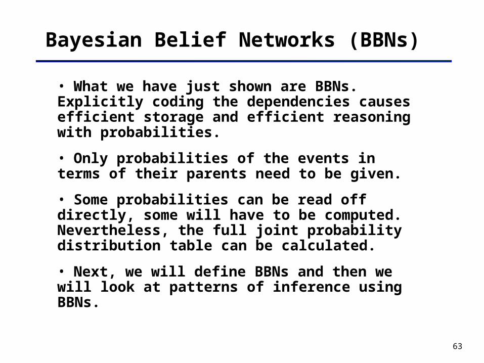
Bayesian Belief Networks (BBNs)
• What we have just shown are BBNs. Explicitly coding the dependencies causes efficient storage and efficient reasoning with probabilities.
• Only probabilities of the events in terms of their parents need to be given.
• Some probabilities can be read off directly, some will have to be computed. Nevertheless, the full joint probability distribution table can be calculated.
• Next, we will define BBNs and then we will look at patterns of inference using BBNs.

64
A belief network is a graph for which the following holds (Russell & Norvig, 2003)
1. A set of random variables makes up the nodes of the network. Variables may be discrete or continuous. Each node is annotated with quantitative probability information.
2. A set of directed links or arrows connects pairs of nodes. If there is an arrow from node X to node Y, X is said to be a parent of Y.
3. Each node Xi has a conditional probability distribution P(Xi | Parents (Xi)) that quantifies the effect of the parents on the node.
4. The graph has no directed cycles (and hence is a directed, acyclic graph, or DAG).
65
More on BBNs
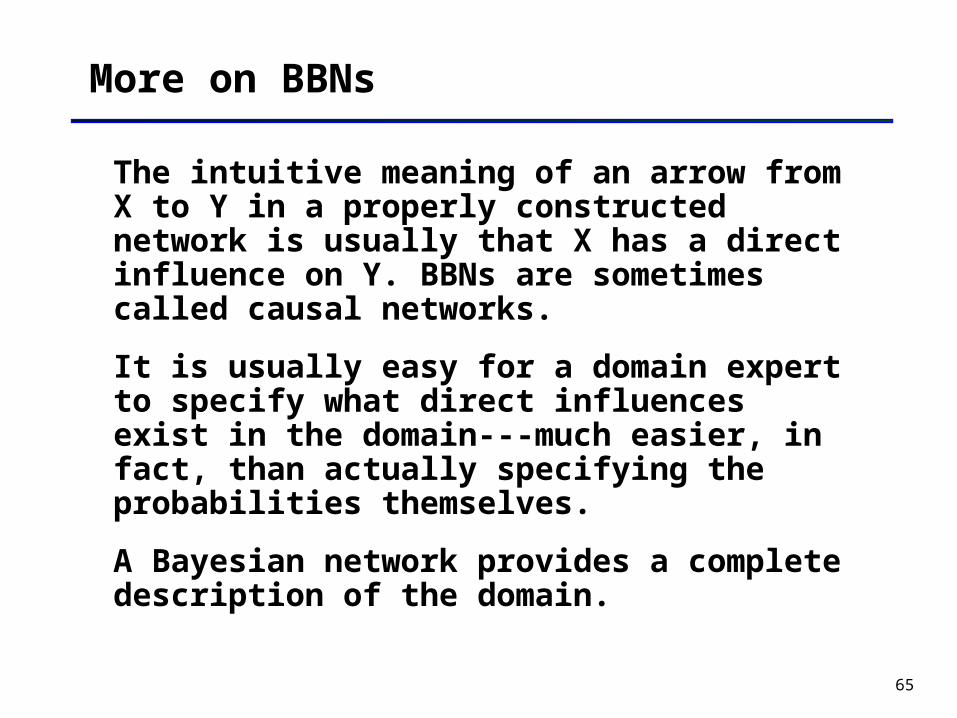
The intuitive meaning of an arrow from X to Y in a properly constructed network is usually that X has a direct influence on Y. BBNs are sometimes called causal networks.
It is usually easy for a domain expert to specify what direct influences exist in the domain---much easier, in fact, than actually specifying the probabilities themselves.
A Bayesian network provides a complete description of the domain.
66
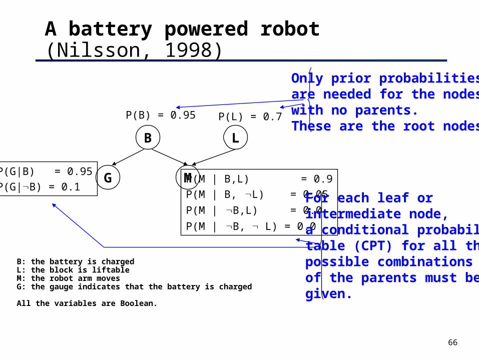
A battery powered robot (Nilsson, 1998)
B: the battery is chargedL: the block is liftableM: the robot arm movesG: the gauge indicates that the battery is charged
All the variables are Boolean.
B L
G M
P(B) = 0.95 P(L) = 0.7
P(G|B) = 0.95
P(G|B) = 0.1
Only prior probabilitiesare needed for the nodes with no parents. These are the root nodes.
P(M | B,L) = 0.9
P(M | B, L) = 0.05
P(M | B,L) = 0.0
P(M | B, L) = 0.0
For each leaf or intermediate node,a conditional probabilitytable (CPT) for all thepossible combinationsof the parents must begiven.
67
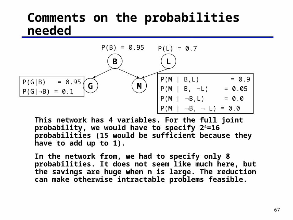
Comments on the probabilities needed
This network has 4 variables. For the full joint probability, we would have to specify 24=16 probabilities (15 would be sufficient because they have to add up to 1).
In the network from, we had to specify only 8 probabilities. It does not seem like much here, but the savings are huge when n is large. The reduction can make otherwise intractable problems feasible.
B L
G M
P(B) = 0.95 P(L) = 0.7
P(G|B) = 0.95
P(G|B) = 0.1
P(M | B,L) = 0.9
P(M | B, L) = 0.05
P(M | B,L) = 0.0
P(M | B, L) = 0.0
68
Some useful rules before we proceed
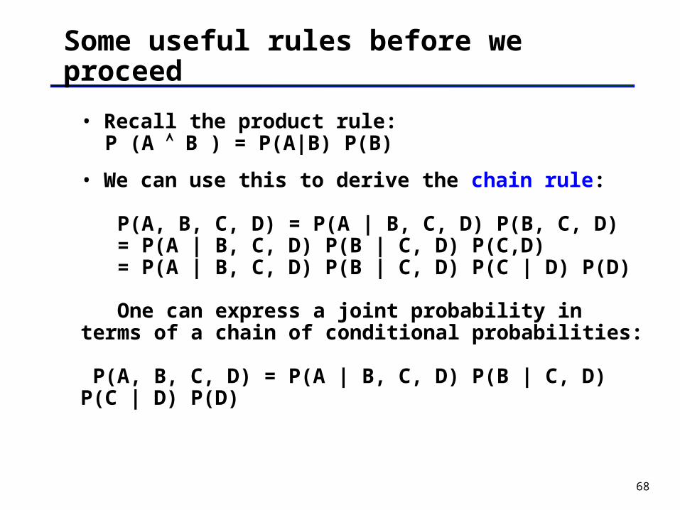
• Recall the product rule: P (A B ) = P(A|B) P(B)
• We can use this to derive the chain rule:
P(A, B, C, D) = P(A | B, C, D) P(B, C, D) = P(A | B, C, D) P(B | C, D) P(C,D) = P(A | B, C, D) P(B | C, D) P(C | D) P(D)
One can express a joint probability in terms of a chain of conditional probabilities:
P(A, B, C, D) = P(A | B, C, D) P(B | C, D) P(C | D) P(D)

69
Some useful rules before we proceed (cont’d)
• How to switch around the conditional:
P (A,B | C) = P(A,B,C) / P(C)
= P(A | B,C) P(B|C) P(C) / P(C) by the chain rule = P(A | B,C) P(B|C) delete P(C)
So, P (A,B | C) = P(A | B,C) P(B|C)

70
Calculating joint probabilities
What is P(G,B,M,L)?
= P(G,M,B,L) order so that lowernodes are first
= P(G|M,B,L) P(M|B,L) P(B|L) P(L) by the chain rule= P(G|B) P(M|B,L) P(B) P(L) nodes need to be
conditioned only ontheir parents
= 0.95 x 0.9 x 0.95 x 0.7 = 0.57 read values from the BBN
B L
G M
P(B) = 0.95 P(L) = 0.7
P(G|B) = 0.95
P(G|B) = 0.1
P(M | B,L) = 0.9
P(M | B, L) = 0.05
P(M | B,L) = 0.0
P(M | B, L) = 0.0

71
Calculating joint probabilities
What is P(G,B,M,L)?
= P(G, M,B,L) order so that lowernodes are first
= P(G| M,B,L) P( M|B,L) P(B|L)P(L) by the chain rule= P(G|B) P( M|B,L) P(B) P(L) nodes need to be
conditioned only ontheir parents
= 0.95 x 0.1 x 0.95 x 0.7 = 0.06 0.1 is 1 - 0.9
B L
G M
P(B) = 0.95 P(L) = 0.7
P(G|B) = 0.95
P(G|B) = 0.1
P(M | B,L) = 0.9
P(M | B, L) = 0.05
P(M | B,L) = 0.0
P(M | B, L) = 0.0

72
Causal or top-down inference
What is P(M | L)?
= P(M,B | L) + P(M, B | L) we want to mention the other parent too
= P(M | B,L) P(B | L) + by a form of the P(M | B,L) P(B | L) chain rule= P(M | B,L) P(B) + from the structure of the P(M | B,L) P(B) network
= 0.9 x 0.95 + 0 x 0.05 = 0.855
B L
G M
P(B) = 0.95 P(L) = 0.7
P(G|B) = 0.95
P(G|B) = 0.1
P(M | B,L) = 0.9
P(M | B, L) = 0.05
P(M | B,L) = 0.0
P(M | B, L) = 0.0

73
Procedure for causal inference
• Rewrite the desired conditional probability of the query node, V, given the evidence, in terms of the joint probability of V and all of its parents (that are not evidence) ,given the evidence.
• Reexpress this joint probability back to the probability of V conditioned on all of the parents.

74
Diagnostic or bottom-up inference
What is P( L | M)?
= P( M | L) P( L) / P( M) by Bayes’ rule = 0.9525 x P( L) / P( M) by causal inference (*)= 0.9525 x 0.3 / P(M) read from the table= 0.9525 x 0.3 / 0.38725 = 0.7379We calculate P(M) by
noticing thatP( L | M) + P( L | M) = 1. (***) (**)
(*) (**) (***) See the following slides.
B L
G M
P(B) = 0.95 P(L) = 0.7
P(G|B) = 0.95
P(G|B) = 0.1
P(M | B,L) = 0.9
P(M | B, L) = 0.05
P(M | B,L) = 0.0
P(M | B, L) = 0.0

75
Diagnostic or bottom-up inference (calculations needed)
• (*) P( M | L) use causal inference= P(M, B | L ) + P(M, B, L)= P(M|B, L) P(B | L) + P(M| B, L) P( B | L) = P(M|B, L) P(B ) + P(M| B, L) P( B )= (1 - 0.05) x 0.95 + 1 * 0.05= 0.95 * 0.95 + 0.05 = 0.9525
• (**) P(L | M ) use Bayes’ rule= P( M | L) P(L) / P( M )= (1 - P(M |L)) P(L) / P( M ) P(M|L) was calculated before= (1 - 0.855) x 0.7 / P( M )= 0.145 x 0.7 / P( M )= 0.1015 / P( M )

76
Diagnostic or bottom-up inference (calculations needed)
• (***) P( L | M ) + P(L | M ) = 1 0.9525 x 0.3 / P(M) + 0.145 x 0.7 / P( M ) = 1 0.28575 / P(M) + 0.1015 / P(M) = 1 P(M) = 0.38725 = (1 - P(M |L)) P(L) / P( M ) P(M|L) was calculated before= (1 - 0.855) x 0.7 / P( M )= 0.145 x 0.7 / P( M )= 0.1015 / P( M )
77
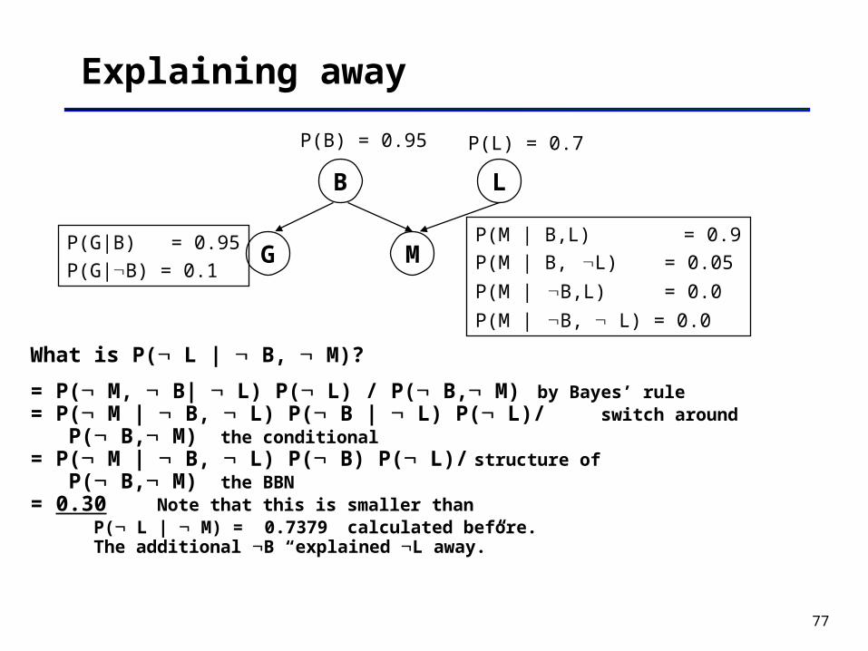
Explaining away
What is P( L | B, M)?
= P( M, B| L) P( L) / P( B, M) by Bayes’ rule = P( M | B, L) P( B | L) P( L)/ switch around P( B, M) the conditional= P( M | B, L) P( B) P( L)/ structure of P( B, M) the BBN= 0.30 Note that this is smaller than
P( L | M) = 0.7379 calculated before.The additional B “explained L away.”
B L
G M
P(B) = 0.95 P(L) = 0.7
P(G|B) = 0.95
P(G|B) = 0.1
P(M | B,L) = 0.9
P(M | B, L) = 0.05
P(M | B,L) = 0.0
P(M | B, L) = 0.0
78
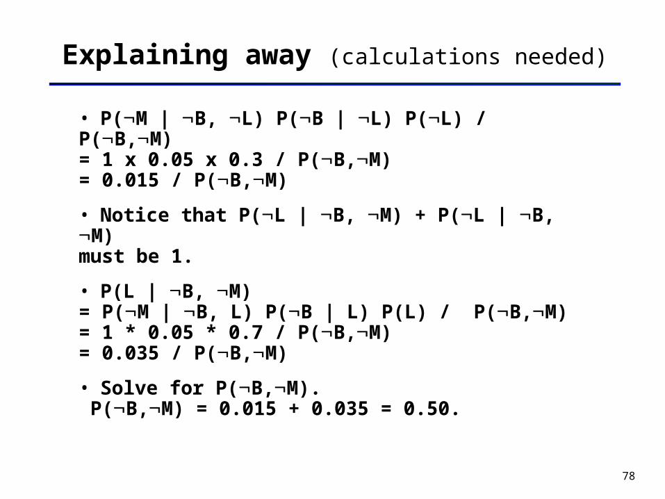
Explaining away (calculations needed)
• P(M | B, L) P(B | L) P(L) / P(B,M) = 1 x 0.05 x 0.3 / P(B,M) = 0.015 / P(B,M)
• Notice that P(L | B, M) + P(L | B, M)must be 1.
• P(L | B, M) = P(M | B, L) P(B | L) P(L) / P(B,M) = 1 * 0.05 * 0.7 / P(B,M) = 0.035 / P(B,M)
• Solve for P(B,M). P(B,M) = 0.015 + 0.035 = 0.50.

79
The fuzzy set representation for “small integers”
80
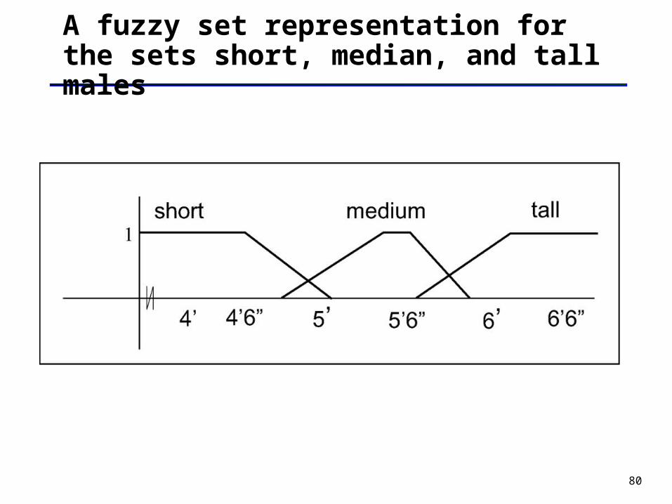
A fuzzy set representation for the sets short, median, and tall males
81
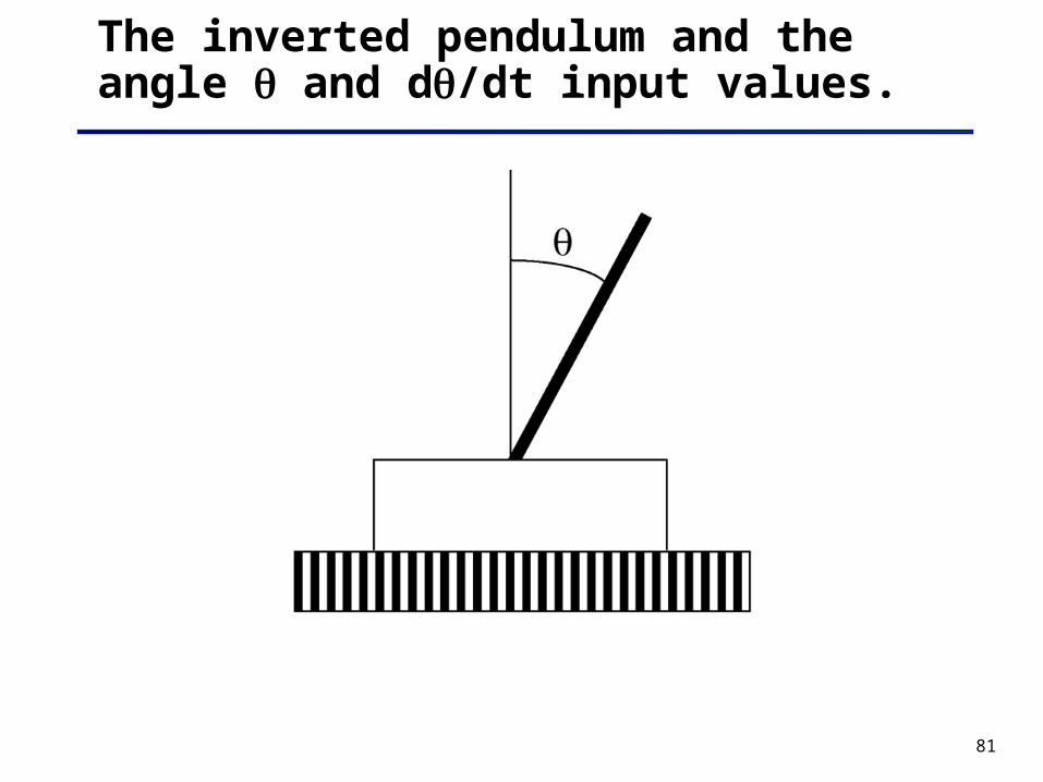
The inverted pendulum and the angle and d/dt input values.

82
The fuzzy regions for the input values (a) and d/dt (b)

83
The fuzzy regions of the output value u, indicating the movement of the pendulum base

84
The fuzzification of the input measures x1=1, x2 = -4

85
The Fuzzy Associative Matrix (FAM) for the pendulum problem
86
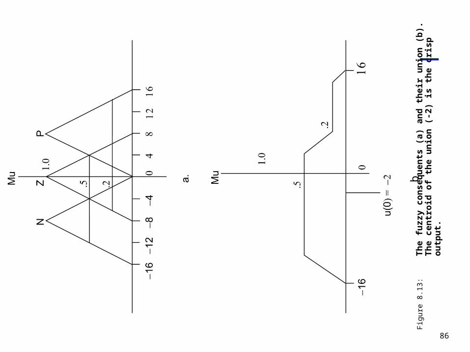
Fig
ure
8.13
:T
he
fuzz
y co
nse
qu
ents
(a)
an
d t
hei
r u
nio
n (
b).
Th
e ce
ntr
oid
of
the
un
ion
(-2
) is
th
e cr
isp
ou
tpu
t.

87
The fuzzy consequents (a), and their union (b)
The centroid of the union (-2) is the crisp output.

88
Minimum of their measures is taken as the measure of the rule result

89
Using Dempster’s rule to obtain a belief distribution for m3

90
Using Dempster’s rule to combine m3 and m4 to get m5