1

Program AnalysisSystematic Domain Design

Mooly Sagivhttp://www.cs.tau.ac.il/~msagiv/courses/pa04.html

Tel Aviv University

640-6706

Textbook: Principles of Program Analysis

Chapter 4, CC79, CC92

2

Outline

Domains with infinite heights Systematic construction of Galois connection Precision

3

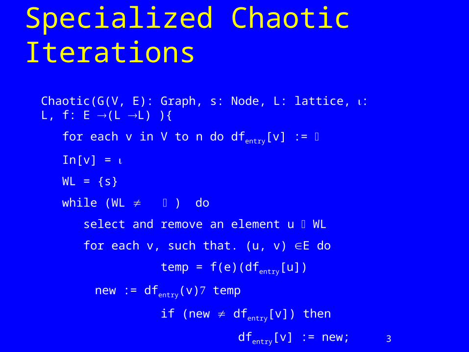
Specialized Chaotic Iterations

Chaotic(G(V, E): Graph, s: Node, L: lattice, : L, f: E (L L) ){

for each v in V to n do dfentry[v] :=

In[v] =

WL = {s}

while (WL ) do

select and remove an element u WL

for each v, such that. (u, v) E do

temp = f(e)(dfentry[u])

new := dfentry(v) temp

if (new dfentry[v]) then

dfentry[v] := new;

WL := WL {v}

4

Widening

Accelerate the termination of Chaotic iterations by computing a more conservative solution

Can handle lattices of infinite heights

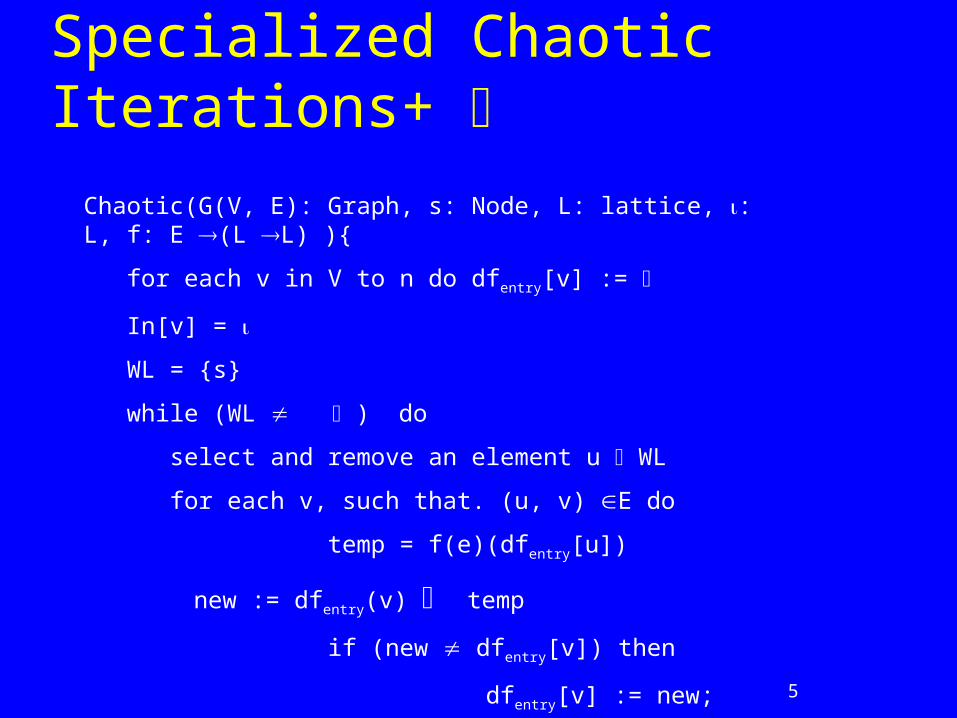
5

Specialized Chaotic Iterations+ Chaotic(G(V, E): Graph, s: Node, L: lattice, : L, f: E (L L) ){

for each v in V to n do dfentry[v] :=

In[v] =

WL = {s}

while (WL ) do

select and remove an element u WL

for each v, such that. (u, v) E do

temp = f(e)(dfentry[u])

new := dfentry(v) temp

if (new dfentry[v]) then

dfentry[v] := new;

WL := WL {v}

6

Example Interval Analysis Find a lower and an upper bound of the value of a

variable Usages? Lattice

L = (Z{-, }Z {-, }, , , , ,)– [a, b] [c, d] if c a and d b– [a, b] [c, d] = [min(a, c), max(b, d)]

– [a, b] [c, d] = [max(a, c), min(b, d)] = =

Galois connection

7

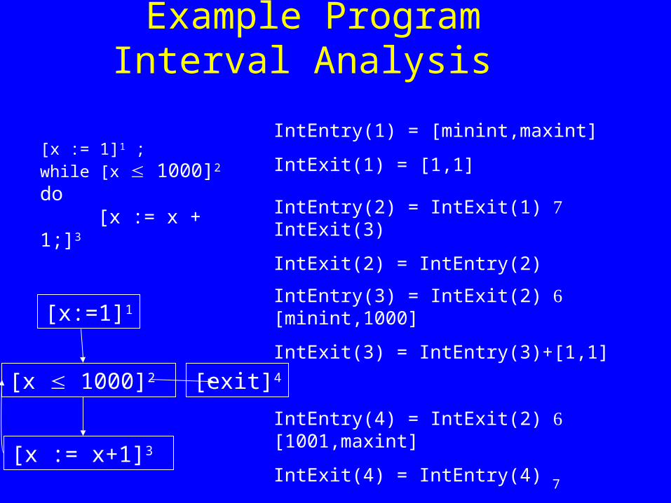
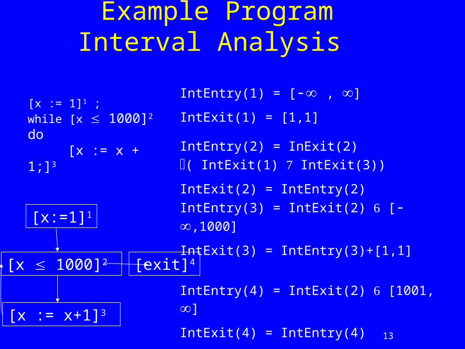
Example ProgramInterval Analysis

[x := 1]1 ;while [x 1000]2 do [x := x + 1;]3

IntEntry(1) = [minint,maxint]

IntExit(1) = [1,1]

IntEntry(2) = IntExit(1) IntExit(3)

IntExit(2) = IntEntry(2)

[x:=1]1

[x 1000]2

[x := x+1]3

[exit]4

IntEntry(3) = IntExit(2) [minint,1000]

IntExit(3) = IntEntry(3)+[1,1]

IntEntry(4) = IntExit(2) [1001,maxint]

IntExit(4) = IntEntry(4)

8

Widening for Interval Analysis [c, d] = [c, d] [a, b] [c, d] = [

if a cthen aelse -,

if b dthen belse

]

9

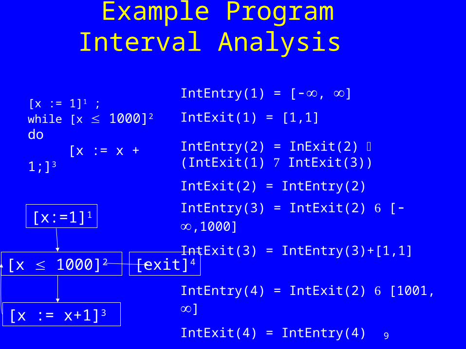
Example ProgramInterval Analysis

[x := 1]1 ;while [x 1000]2 do [x := x + 1;]3

IntEntry(1) = [-, ]

IntExit(1) = [1,1]

IntEntry(2) = InExit(2) (IntExit(1) IntExit(3))

IntExit(2) = IntEntry(2)

[x:=1]1

[x 1000]2

[x := x+1]3

[exit]4

IntEntry(3) = IntExit(2) [-,1000]

IntExit(3) = IntEntry(3)+[1,1]

IntEntry(4) = IntExit(2) [1001, ]

IntExit(4) = IntEntry(4)

10

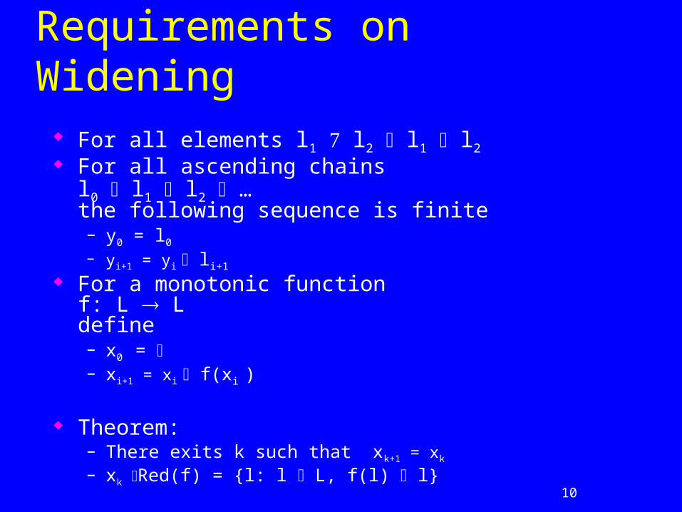
Requirements on Widening For all elements l1 l2 l1 l2 For all ascending chains

l0 l1 l2 …the following sequence is finite– y0 = l0 – yi+1 = yi li+1

For a monotonic function f: L Ldefine– x0 = – xi+1 = xi f(xi )

Theorem:– There exits k such that xk+1 = xk

– xk Red(f) = {l: l L, f(l) l}

11

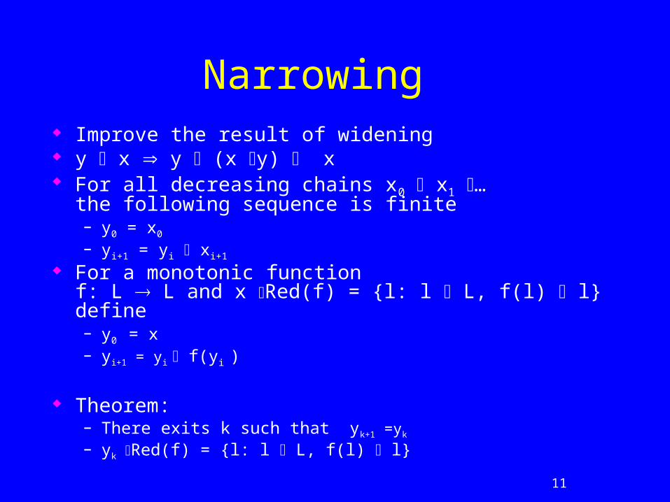
Narrowing Improve the result of widening y x y (x y) x For all decreasing chains x0 x1 …

the following sequence is finite– y0 = x0

– yi+1 = yi xi+1

For a monotonic function f: L L and x Red(f) = {l: l L, f(l) l}define– y0 = x– yi+1 = yi f(yi )

Theorem:– There exits k such that yk+1 =yk

– yk Red(f) = {l: l L, f(l) l}

12

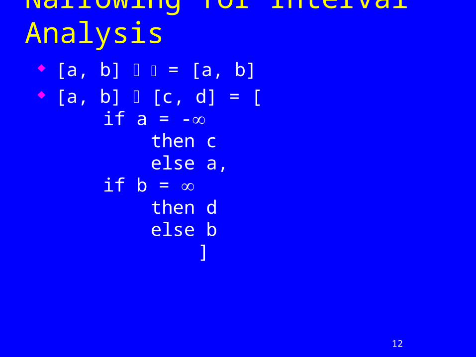
Narrowing for Interval Analysis [a, b] = [a, b] [a, b] [c, d] = [

if a = - then celse a,

if b = then delse b

]

13

Example ProgramInterval Analysis

[x := 1]1 ;while [x 1000]2 do [x := x + 1;]3

IntEntry(1) = [- , ]

IntExit(1) = [1,1]

IntEntry(2) = InExit(2) ( IntExit(1) IntExit(3))

IntExit(2) = IntEntry(2)

[x:=1]1

[x 1000]2

[x := x+1]3

[exit]4

IntEntry(3) = IntExit(2) [-,1000]

IntExit(3) = IntEntry(3)+[1,1]

IntEntry(4) = IntExit(2) [1001, ]

IntExit(4) = IntEntry(4)

14

Non Montonicity of Widening

15

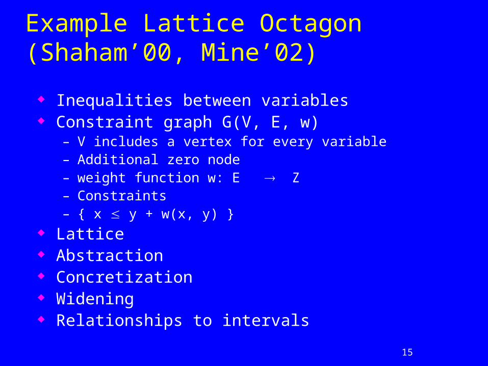
Example Lattice Octagon (Shaham’00, Mine’02)

Inequalities between variables Constraint graph G(V, E, w)

– V includes a vertex for every variable– Additional zero node– weight function w: E Z – Constraints– { x y + w(x, y) }

Lattice Abstraction Concretization Widening Relationships to intervals

16

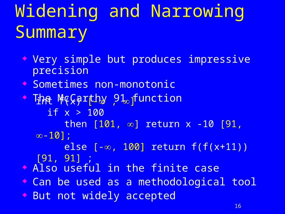
Widening and Narrowing Summary

Very simple but produces impressive precision Sometimes non-monotonic The McCarthy 91 function

Also useful in the finite case Can be used as a methodological tool But not widely accepted

int f(x) [- , ] if x > 100 then [101, ] return x -10 [91, -10]; else [-, 100] return f(f(x+11)) [91, 91] ;

17

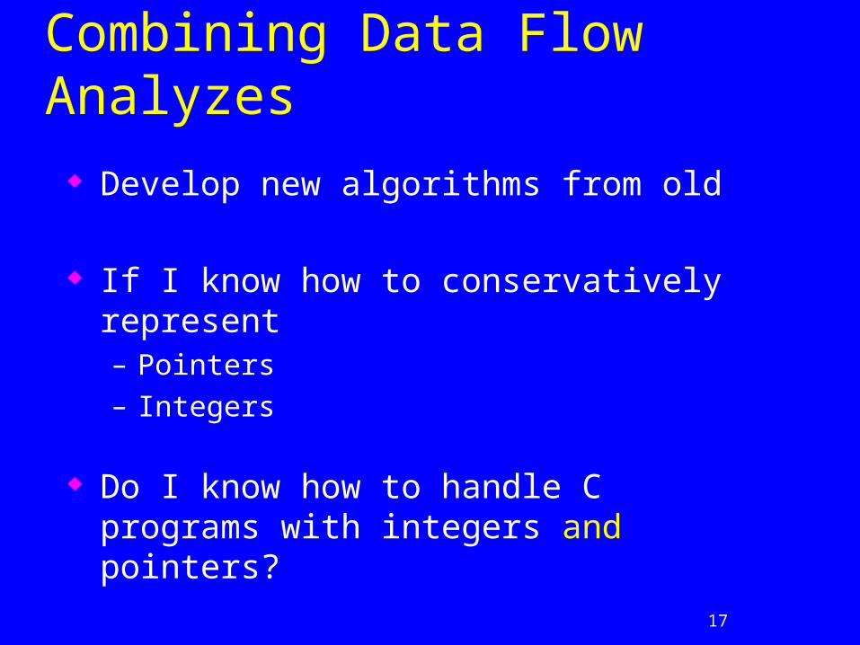
Combining Data Flow Analyzes

Develop new algorithms from old

If I know how to conservatively represent – Pointers

– Integers

Do I know how to handle C programs with integers and pointers?

18

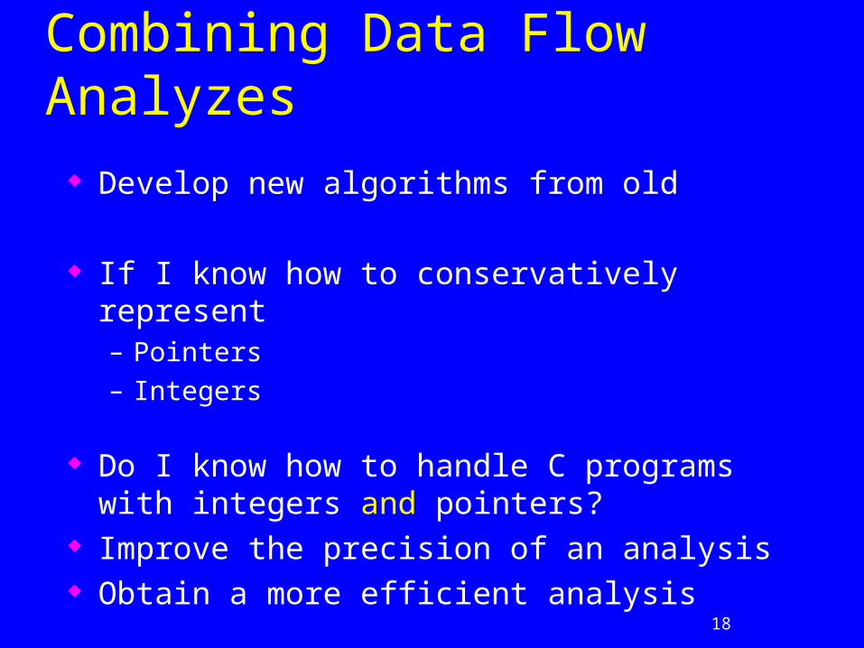
Combining Data Flow Analyzes

Develop new algorithms from old

If I know how to conservatively represent – Pointers

– Integers

Do I know how to handle C programs with integers and pointers?

Improve the precision of an analysis Obtain a more efficient analysis

19

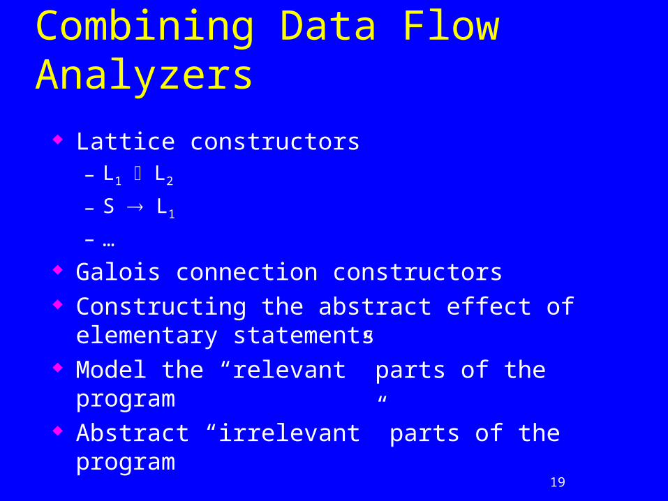
Combining Data Flow Analyzers

Lattice constructors– L1 L2

– S L1

– …

Galois connection constructors Constructing the abstract effect of elementary

statements Model the “relevant” parts of the program Abstract “irrelevant” parts of the program

20

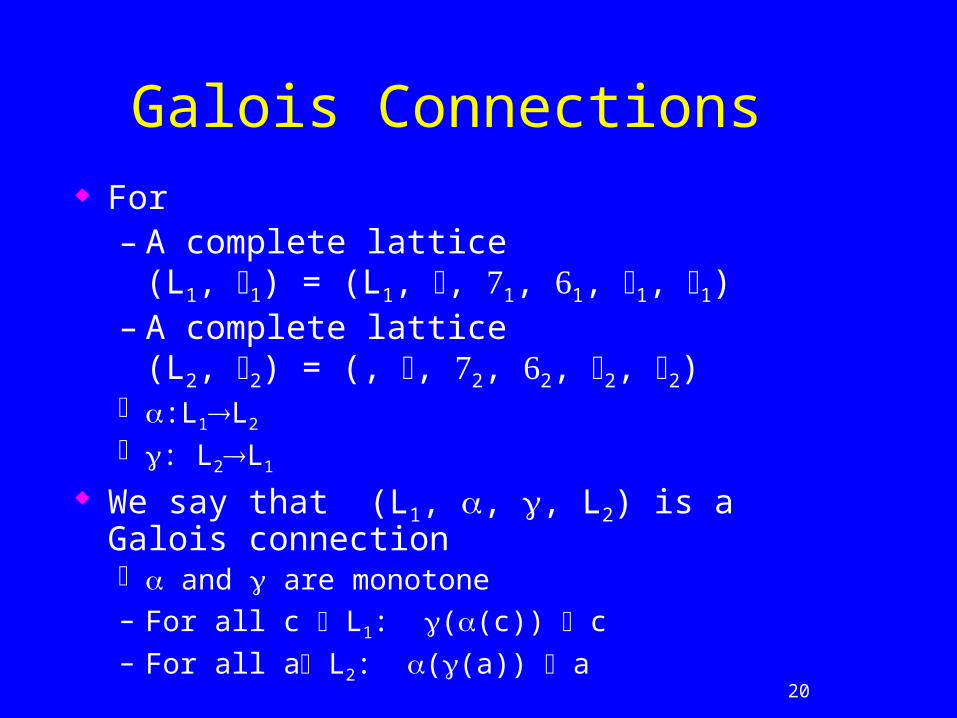
Galois Connections For

– A complete lattice (L1, 1) = (L1, , 1, 1, 1, 1)

– A complete lattice (L2, 2) = (, , 2, 2, 2, 2)

:L1L2

: L2L1

We say that (L1, , , L2) is a Galois connection and are monotone– For all c L1: ((c)) c– For all a L2: ((a)) a

21

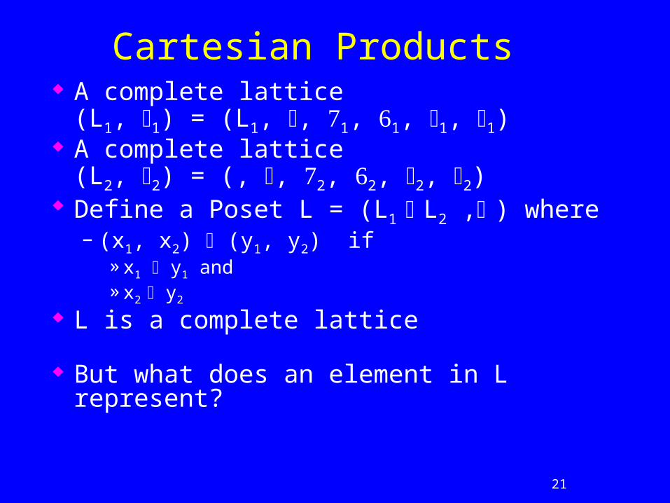
Cartesian Products A complete lattice

(L1, 1) = (L1, , 1, 1, 1, 1) A complete lattice

(L2, 2) = (, , 2, 2, 2, 2) Define a Poset L = (L1 L2 , ) where

– (x1, x2) (y1, y2) if » x1 y1 and» x2 y2

L is a complete lattice

But what does an element in L represent?

22

Cartesian Products (cont) A complete lattice

(L1, 1) = (L1, , 1, 1, 1, 1) A complete lattice

(L2, 2) = (, , 2, 2, 2, 2) Complete lattice L = (L1 L2 , ) A concrete lattice C (usually a powerset) A Galois connection

(C, 1 , 1, L1) A Galois connection

(C, 2 , 2, L2) Define :C L1 L2 and : L1 L2 C ? Example: Parity Sign

23

Cartesian Products (cont) A Galois connection

(C, 1 , 1, L1) A Galois connection

(C, 2 , 2, L2) A Galois connection (C, , , L1 L2 )

(c) = <1(c), 2(c)> (<a1, a2>) = 1(a1) 2(a2)

Define – L1st#: L1 L1

– L2st#: L2 L2

How to define L1 L2 st#: L1 L2 L1 L2 – Preserve soundness– Preserve relative optimality (induced)

Example: Parity Sign

24

Component-wise combinations

Combine several analyses into a single analysis Cartesian products (Direct product) Independent attribute method Relational attribute method Total function space Monotone function space Direct tensor product

25

Independent Attribute Method A Galois connection

(C1, 1 , 1, L1) A Galois connection

(C2, 2 , 2, L2) A Galois connection (C1C2, , , L1 L2 )

(<c1, c2>) = <1(c1), 2(c2)> (<a1, a2>) = <1(a1) , 2(a2)>

Define – L1st#: L1 L1

– L2st#: L2 L2

How to define L1 L2 st#: L1 L2 L1 L2 – Preserve soundness– Preserve relative optimality (induced)

26

Relational Attribute Method A Galois connection

(P(C1), 1 , 1, P(L1)) where 1: C1L1

– 1 (X) = {1(c) | c X}

A Galois connection(P(C2), 2 , 2, P(L2)) where 2: C2L2

2 (X) = {2(c) | c X}

A Galois connection (P(C1C2), , , P(L1 L2)) (<X1, X2>) = {<1(c1), 2(c2)> | c1 X1, c2 X2}

(<Y1,Y2>) = {<c1 , c2> | 1(c1) Y1 2(c2) Y2 }

But how about transformers?

27

Conclusions(1)

Good static analysis = – Precise enough (for the client)

– Efficient enough

Good static analysis– Good domain

» Abstract non-important details

» Represent relevant concrete information

» Precise and efficient abstract meaning of abstract interpreters

» Efficient join implementation

» Small height or widening

28

Conclusions(2)

The Theory of Static Analysis is well founded– Abstraction

– Soundness

– Chaotic iterations

– Elimination methods

– Modular methods

Weak Parts– Transformations

– Predictable approximations

– System