1

Ordinary Differential Equations

Jyun-Ming Chen

2

Contents

• Review• Euler’s method• 2nd order methods

– Midpoint

– Heun’s

• Runge-Kutta Method

• Systems of ODE• Stability Issue• Implicit Methods• Adaptive Stepsize

3

Review

• DE (Differential Equation)– An equation specifying the relations among the

rate change (derivatives) of variables

• ODE (Ordinary DE) vs. PDE (Partial DE)– The number of independent variables involved

)( 2

2

txxdt

xd ),( 1 yxf

y

f

x

f

4

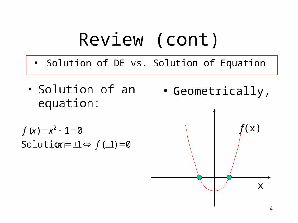
Review (cont)

• Solution of an equation:

• Solution of DE vs. Solution of Equation

0)1(1 :Solution

01)( 2

fx

xxf

• Geometrically,

f(x)

x

5

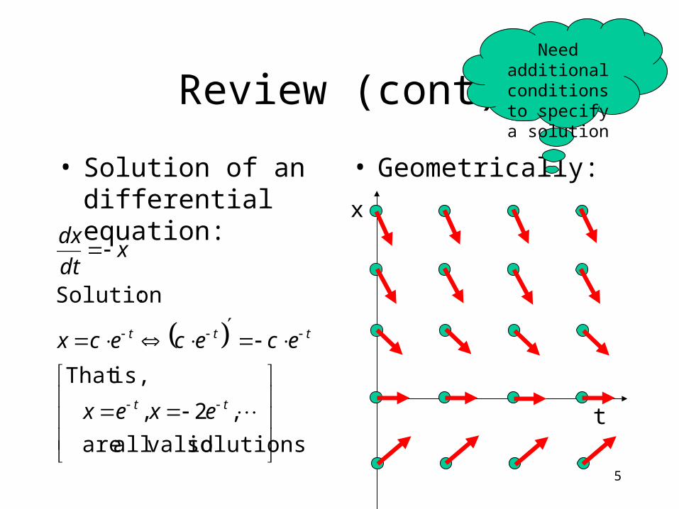
Review (cont)

• Solution of an differential equation:

• Geometrically:

solutions validall are

,2,

is,That

:Solution

tt

ttt

exex

ecececx

xdt

dx

t

x

Need additional conditions to

specify a solution

6

Review (cont)

• Order of an ODE– The highest derivative in the equation

• nth order ODE requires n conditions to specify the solution– IVP (initial value problem): All conditions

specified at the same (initial) point– BVP (boundary value problem): otherwise

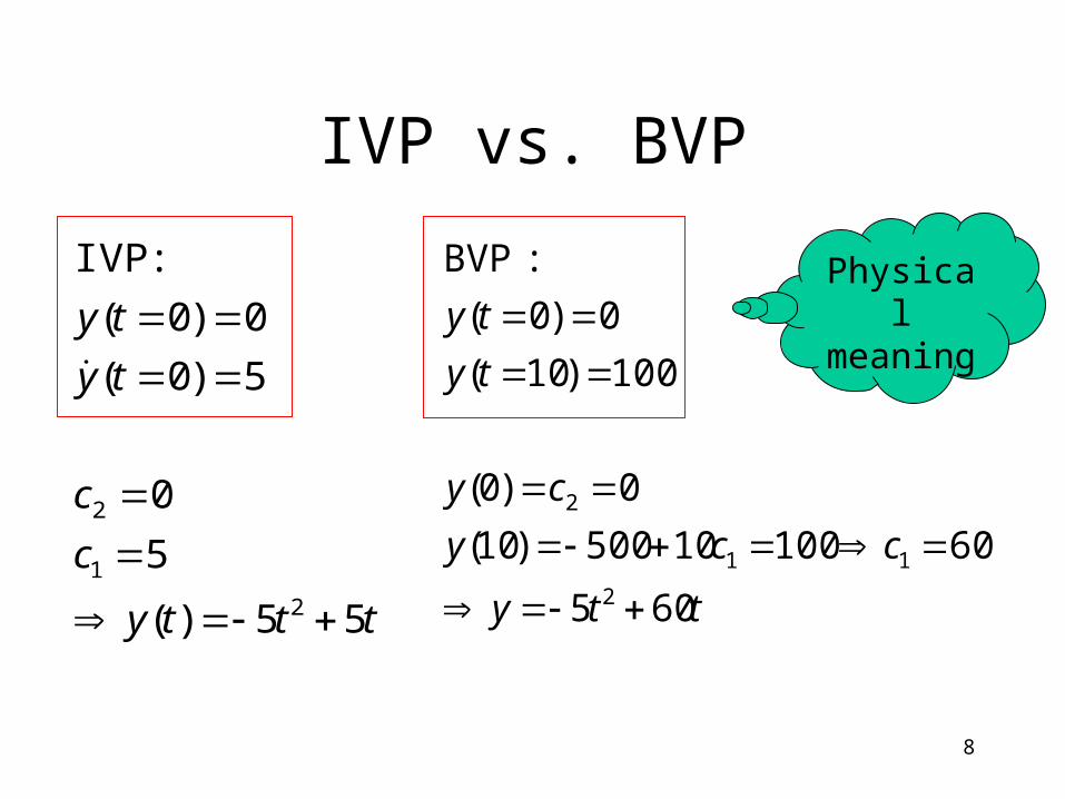
7

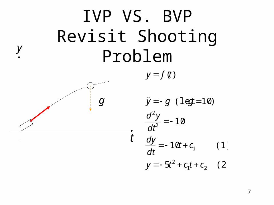
IVP VS. BVPRevisit Shooting Problem

t

g

y

(2) 5

(1) 10

10

)10(let

)(

212

1

2

2

ctcty

ctdt

dydt

yd

ggy

tfy

8

IVP vs. BVP

ttty

c

c

ty

ty

55)(

5

0

5)0(

0)0(

:IVP

2

1

2

tty

ccy

cy

ty

ty

605

6010010500)10(

0)0(

100)10(

0)0(

:BVP

2

11

2

Physical meaning

9

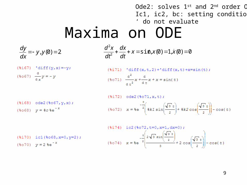
Maxima on ODE

Ode2: solves 1st and 2nd order ODEIc1, ic2, bc: setting conditions‘ do not evaluate

2)0(, yydx

dy0)0(,1)0(,sin

2

2

xxtxdt

dx

dt

xd

10

Linear ODE

• Linearity:– Involves no product nor nonlinear functions of

y and its derivatives

• nth order linear ODE

)()()()()( 011

1

1 xbyxadx

dyxa

dx

ydxa

dx

ydxa

n

n

nn

n

n

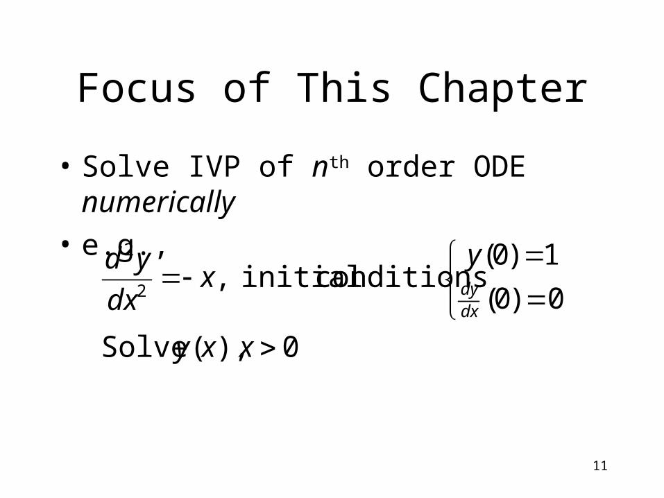
11

Focus of This Chapter

• Solve IVP of nth order ODE numerically

• e.g.,

0 ),( Solve

0)0(

1)0( conditions initial ,

2

2

xxy

yx

dx

yd

dxdy

12

ODE (IVP)

• First order ODE (canonical form)

• Every nth order ODE can be converted to n first order ODEs in the following method:

0)0(),,( yxyyxfdx

dy

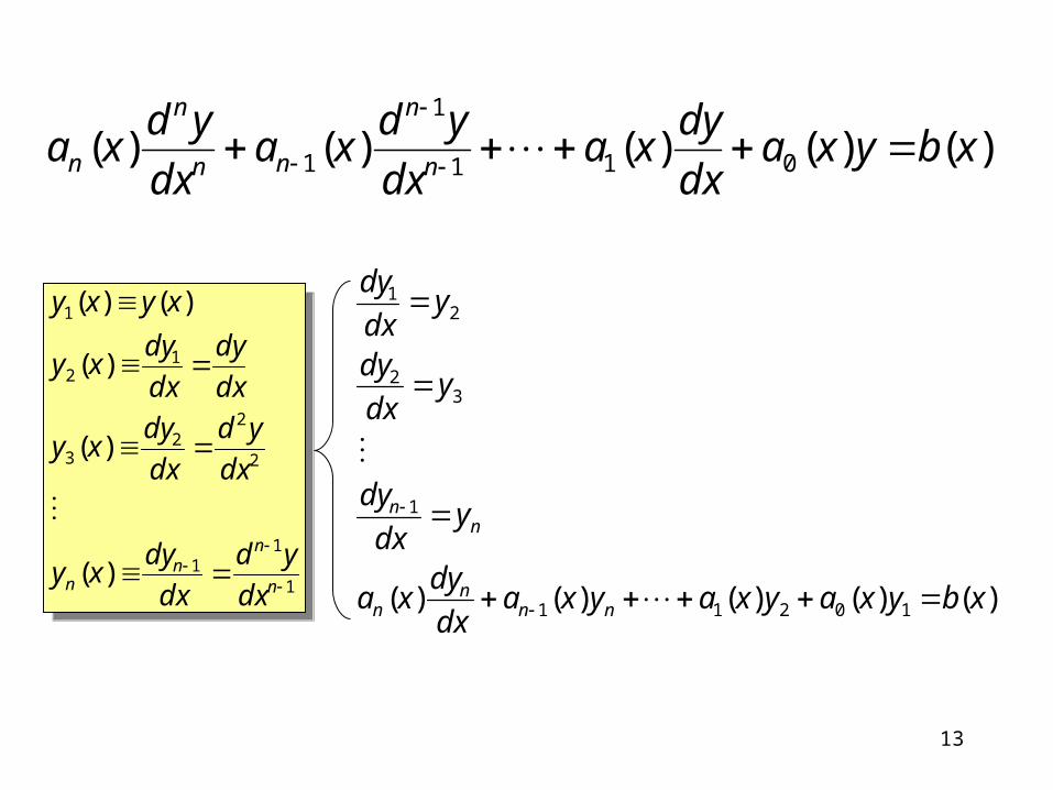
13

)()()()()( 011

1

1 xbyxadx

dyxa

dx

ydxa

dx

ydxa

n

n

nn

n

n

1

11

2

22

3

12

1

)(

)(

)(

)()(

n

nn

n dx

yd

dx

dyxy

dx

yd

dx

dyxy

dx

dy

dx

dyxy

xyxy

1

11

2

22

3

12

1

)(

)(

)(

)()(

n

nn

n dx

yd

dx

dyxy

dx

yd

dx

dyxy

dx

dy

dx

dyxy

xyxy

)()()()()( 10211

1

32

21

xbyxayxayxadx

dyxa

ydx

dy

ydx

dy

ydx

dy

nnn

n

nn

14

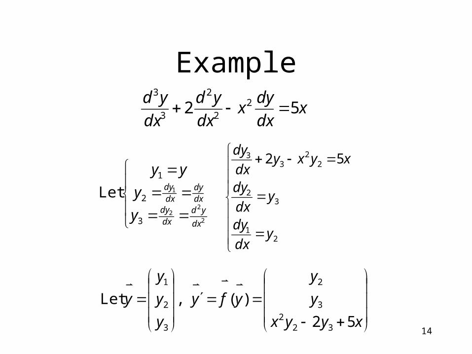
Example

xdx

dyx

dx

yd

dx

yd52 2

2

2

3

3

2

22

1

3

2

1

Let

dx

yddxdy

dxdy

dxdy

y

y

yy

21

32

22

33 52

ydx

dy

ydx

dy

xyxydx

dy

xyyx

y

y

yfy

y

y

y

y

52

)( ,Let

322

3

2

3

2

1

15

End of Review

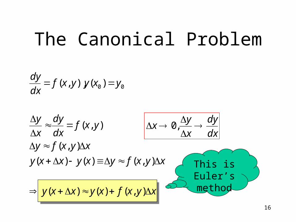
16

xyxfxyxxy

xyxfyxyxxy

xyxfy

yxfdx

dy

x

y

yxyyxfdx

dy

),()()(

),()()(

),(

),(

)(),,( 00

The Canonical Problem

dx

dy

x

yx

,0

This is Euler’s method

17

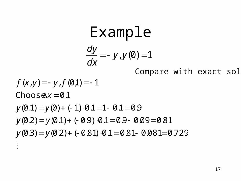
Example

1)0(, yydx

dy

729.0081.081.01.0)81.0()2.0()3.0(

81.009.09.01.0)9.0()1.0()2.0(

9.01.011.0)1()0()1.0(

1.0 Choose

1)1,0(,),(

yy

yy

yy

x

fyyxfCompare with exact sol:

18

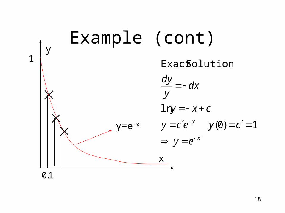
Example (cont)

1)0(

ln

:SolutionExact

x

x

ey

cyecy

cxy

dxy

dy

1.0

1

x

y

y=e–x

19

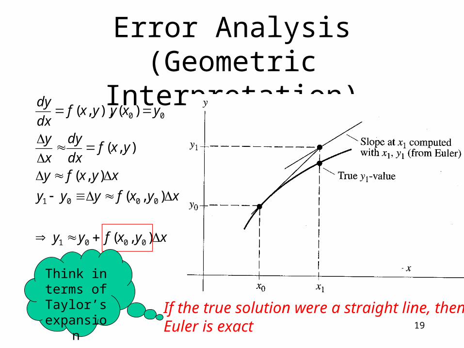
Error Analysis(Geometric Interpretation)

xyxfyy

xyxfyyy

xyxfy

yxfdx

dy

x

y

yxyyxfdx

dy

),(

),(

),(

),(

)(),,(

0001

0001

00

If the true solution were a straight line, thenEuler is exact

Think in terms of Taylor’s

expansion

20

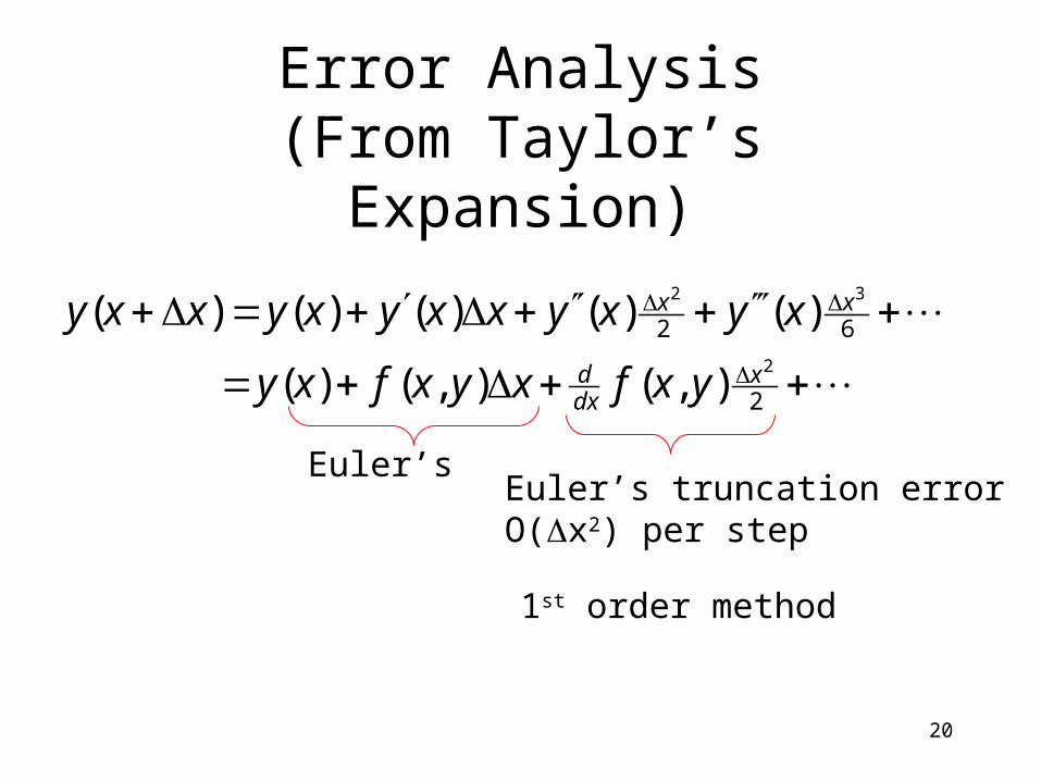
Error Analysis(From Taylor’s Expansion)

2

62

2

32

),(),()(

)()()()()(x

dxd

xx

yxfxyxfxy

xyxyxxyxyxxy

Euler’sEuler’s truncation errorO(x2) per step

1st order method

21

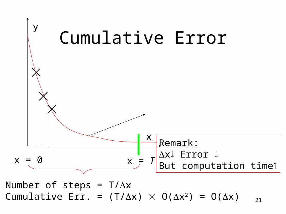
Cumulative Error

x

y

x = 0 x = T

Number of steps = T/xCumulative Err. = (T/x) O(x2) = O(x)

Remark:x Error But computation time

22

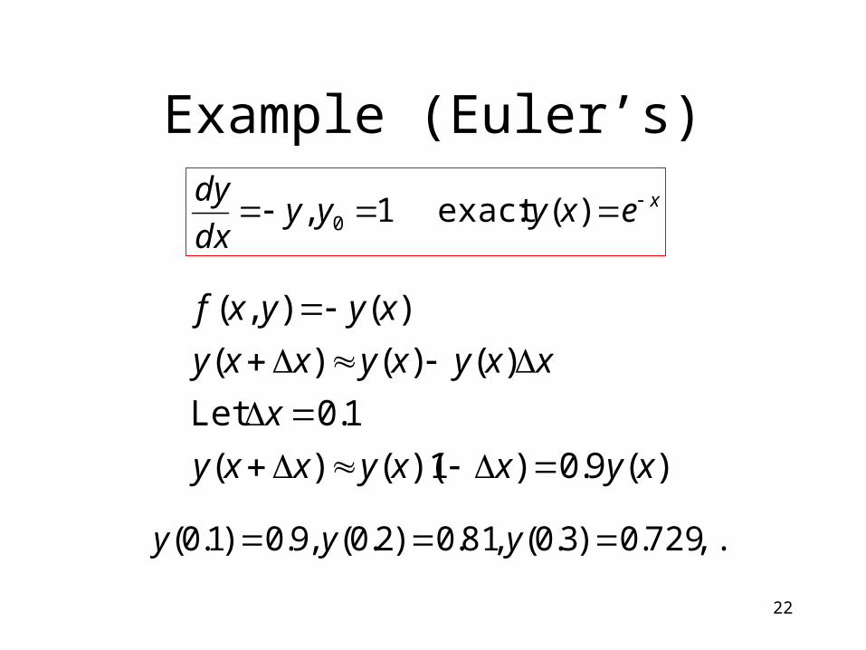
Example (Euler’s)

xexyyydx

dy )(:exact 1, 0

)(9.0)1)(()(

1.0Let

)()()(

)(),(

xyxxyxxy

x

xxyxyxxy

xyyxf

,...729.0)3.0(,81.0)2.0(,9.0)1.0( yyy

23

Methods Improving Euler

Motivated by

Geometric Interpretation

24

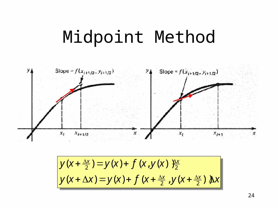
Midpoint Method

xxyxfxyxxy

xyxfxyxyxx

xx

))(,()()(

))(,()()(

22

22

xxyxfxyxxy

xyxfxyxyxx

xx

))(,()()(

))(,()()(

22

22

25

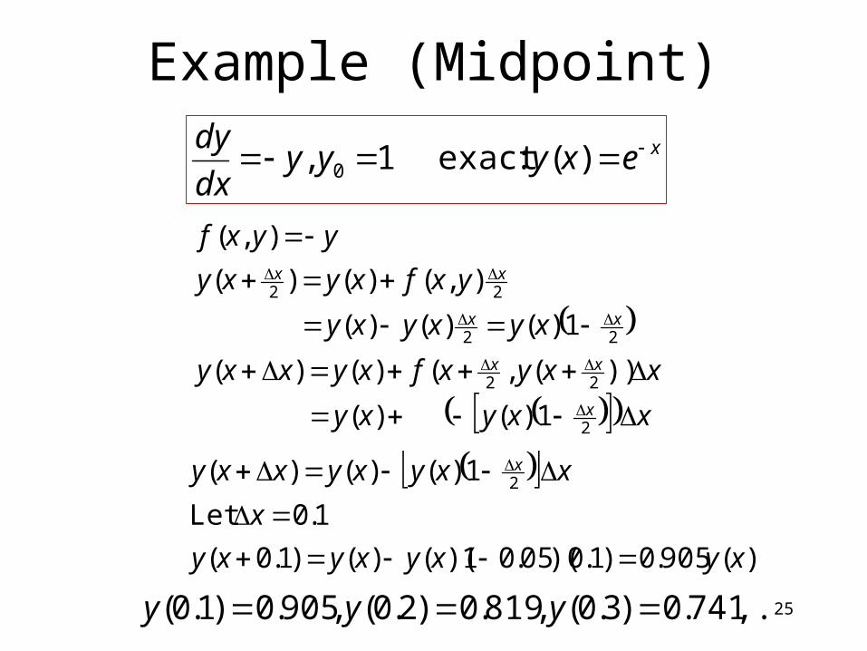
Example (Midpoint)

xxyxy

xxyxfxyxxy

xyxyxy

yxfxyxy

yyxf

x

xx

xx

xx

2

22

22

22

1)( )(

))(,()()(

1)()()(

),()()(

),(

)(905.0)1.0)(05.01)(()()1.0(

1.0Let

1)()()( 2

xyxyxyxy

x

xxyxyxxy x

xexyyydx

dy )(:exact 1, 0

,...741.0)3.0(,819.0)2.0(,905.0)1.0( yyy

26

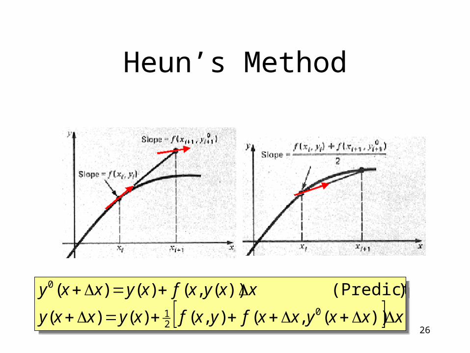
Heun’s Method

xxxyxxfyxfxyxxy

xxyxfxyxxy

))(,(),()()(

)(Predictor ))(,()()(0

21

0

xxxyxxfyxfxyxxy

xxyxfxyxxy

))(,(),()()(

)(Predictor ))(,()()(0

21

0

27

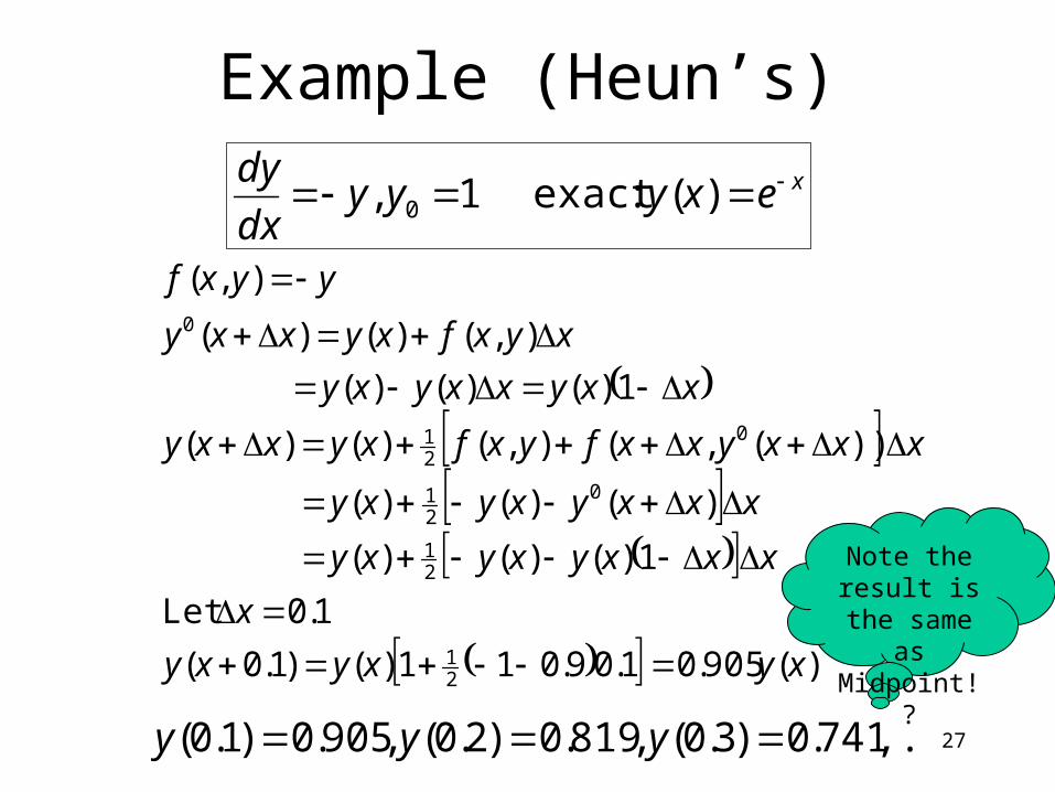
Example (Heun’s)

)(905.01.09.011)()1.0(

1.0Let

1)()()(

)()( )(

))(,(),()()(

1)()()(

),()()(

),(

21

21

021

021

0

xyxyxy

x

xxxyxyxy

xxxyxyxy

xxxyxxfyxfxyxxy

xxyxxyxy

xyxfxyxxy

yyxf

xexyyydx

dy )(:exact 1, 0

,...741.0)3.0(,819.0)2.0(,905.0)1.0( yyy

Note the result is the same as

Midpoint!?

28

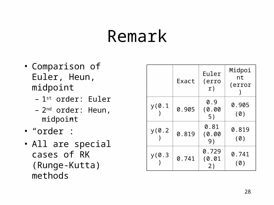
Remark

• Comparison of Euler, Heun, midpoint– 1st order: Euler

– 2nd order: Heun, midpoint

• “order”:• All are special cases of

RK (Runge-Kutta) methods

ExactEuler (error)

Midpoint (error)

y(0.1) 0.9050.9 (0.0

05)0.905

(0)

y(0.2) 0.8190.81 (0.

009)0.819

(0)

y(0.3) 0.7410.729 (0.

012)0.741

(0)

29

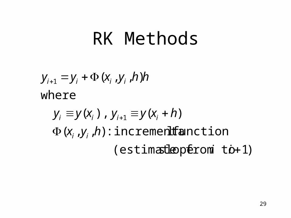
RK Methods

)1 to from slope (estimate

function lincrementa :),,(

)( ),(

where

),,(

1

1

ii

hyx

hxyyxyy

hhyxyy

ii

iiii

iiii

30

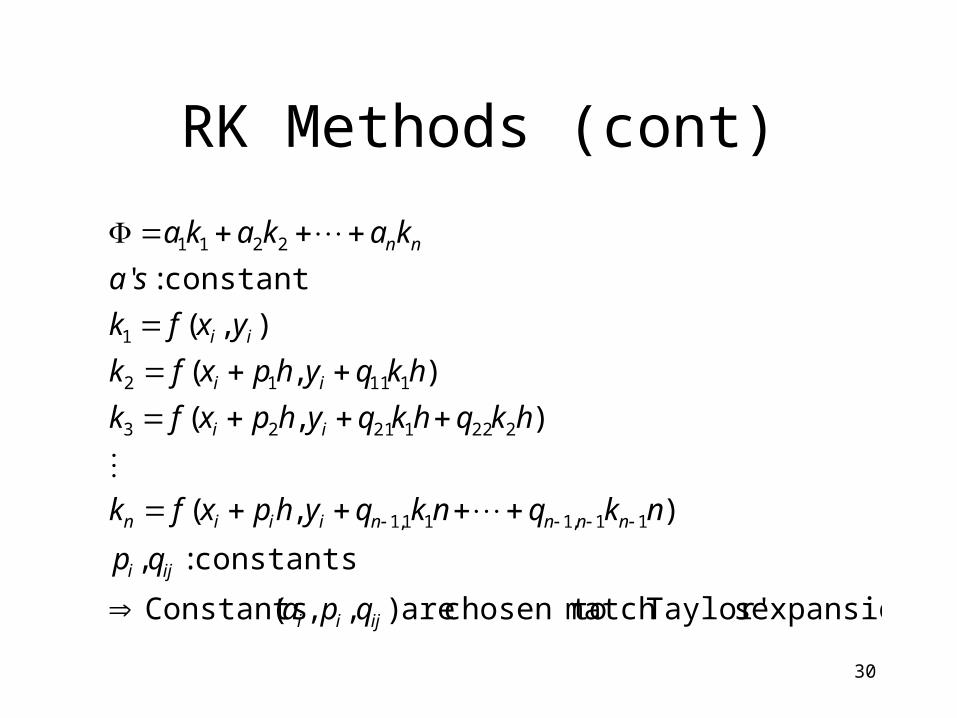
RK Methods (cont)

expansion sTaylor'match chosen to are ),,( Constants

constants:,

),(

),(

),(

),(

constant:'

11,111,1

22212123

11112

1

2211

ijii

iji

nnnniiin

ii

ii

ii

nn

qpa

qp

nkqnkqyhpxfk

hkqhkqyhpxfk

hkqyhpxfk

yxfk

sa

kakaka

31

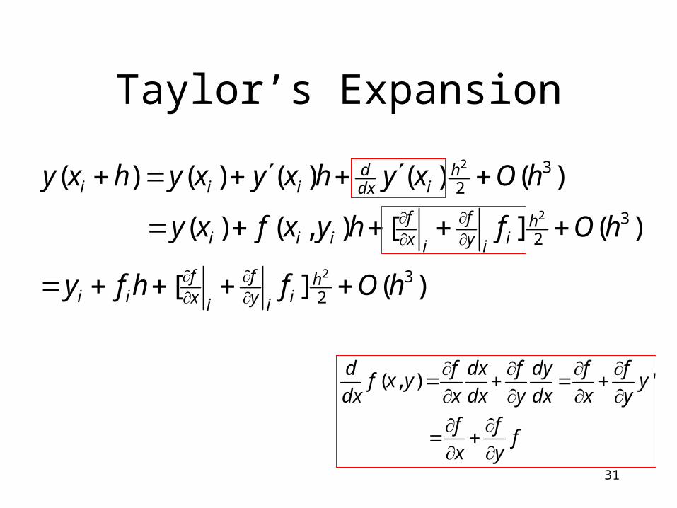
Taylor’s Expansion

fy

f

x

f

yy

f

x

f

dx

dy

y

f

dx

dx

x

fyxf

dx

d

'),(

)(][

)(][),()(

)()()()()(

32

32

32

2

2

2

hOfhfy

hOfhyxfxy

hOxyhxyxyhxy

hiiy

f

ixf

ii

hiiy

f

ixf

iii

hidx

diii

32

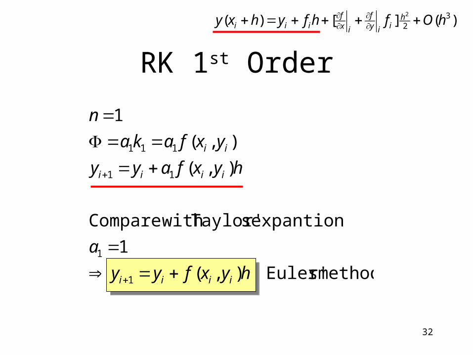
RK 1st Order

method sEuler' ),(

1

expantion sTaylor' with Compare

),(

),(

1

1

1

11

111

hyxfyy

a

hyxfayy

yxfaka

n

iiii

iiii

ii

)(][)( 32

2

hOfhfyhxy hiiy

f

ixf

iii

33

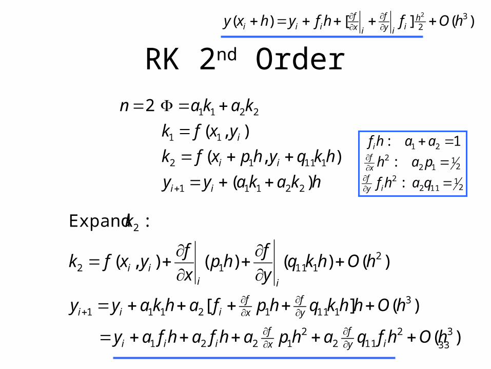
RK 2nd Order

)(

)(][

)()()(),(

: Expand

32112

21221

311112111

211112

2

hOhfqahpahfahfay

hOhhkqhpfahkayy

hOhkqy

fhp

x

fyxfk

k

iyf

xf

iii

yf

xf

iii

iiii

hkakayy

hkqyhpxfk

yxfk

kakan

ii

ii

i

)(

),(

),(

2

22111

11112

11

2211

)(][)( 32

2

hOfhfyhxy hiiy

f

ixf

iii

21

1122

21

122

21

:

:

1 :

qahf

pah

aahf

iyfxfi

34

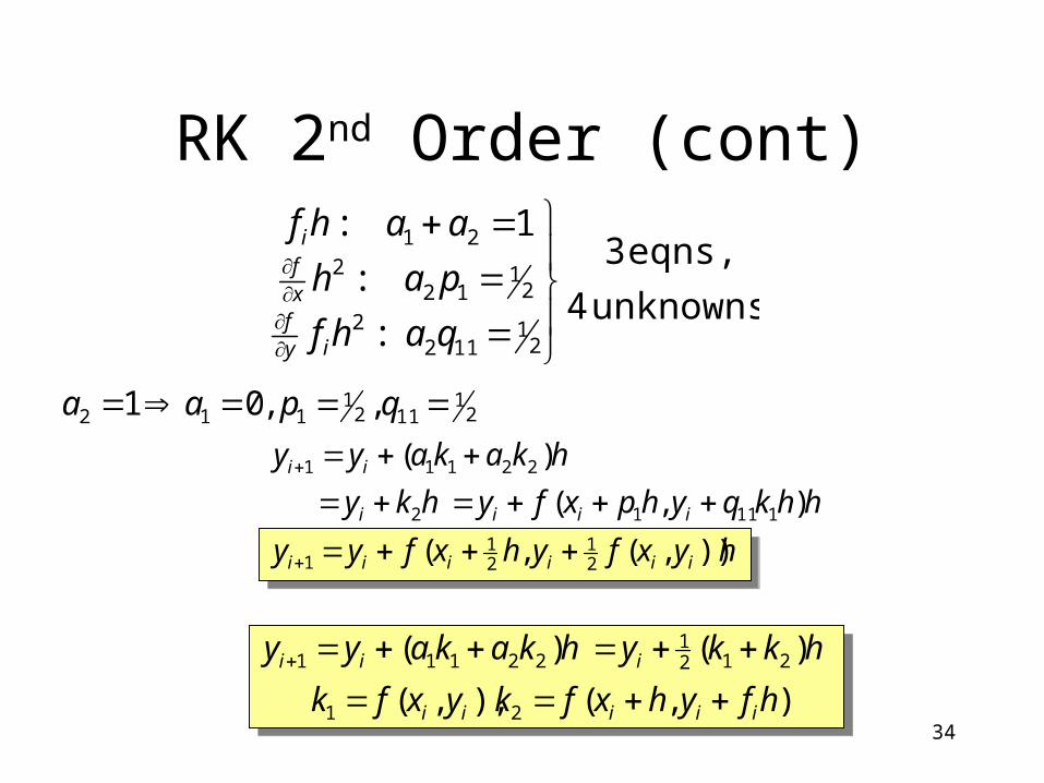
RK 2nd Order (cont)

unknowns 4

eqns, 3

:

:

1 :

21

1122

21

122

21

qahf

pah

aahf

iyfxfi

21

1121

112 , ,01 qpaa

hyxfyhxfyy

hhkqyhpxfyhky

hkakayy

iiiiii

iiii

ii

)),(,(

),(

)(

21

21

1

11112

22111

),(),,(

)( )(

21

2121

22111

hfyhxfkyxfk

hkkyhkakayy

iiiii

iii

35

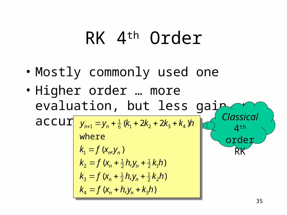
RK 4th Order

• Mostly commonly used one

• Higher order … more evaluation, but less gain on accuracy

Classical 4th order

RK

)(

)(

)(

)(

where

)22(

34

221

21

3

121

21

2

1

432161

1

hkh,yxfk

hkh,yxfk

hkh,yxfk

,yxfk

hkkkkyy

nn

nn

nn

nn

nn

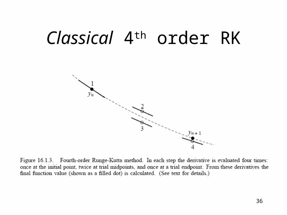
36

Classical 4th order RK

37

System of ODE

• Convert higher order ODE to 1st order ODEs

• All methods equally apply, in vector form

38

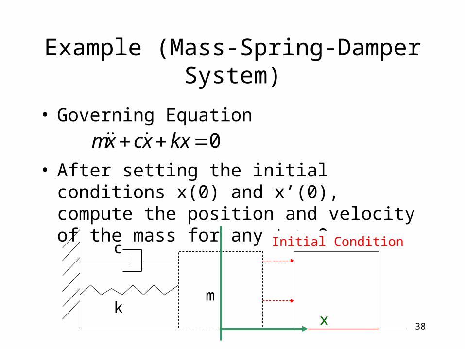
Example (Mass-Spring-Damper System)

• Governing Equation

• After setting the initial conditions x(0) and x’(0), compute the position and velocity of the mass for any t > 0

0 kxxcxm

c

k

Initial Condition

x

m

39

0)0(

1)0(:IC

)(10

then

,

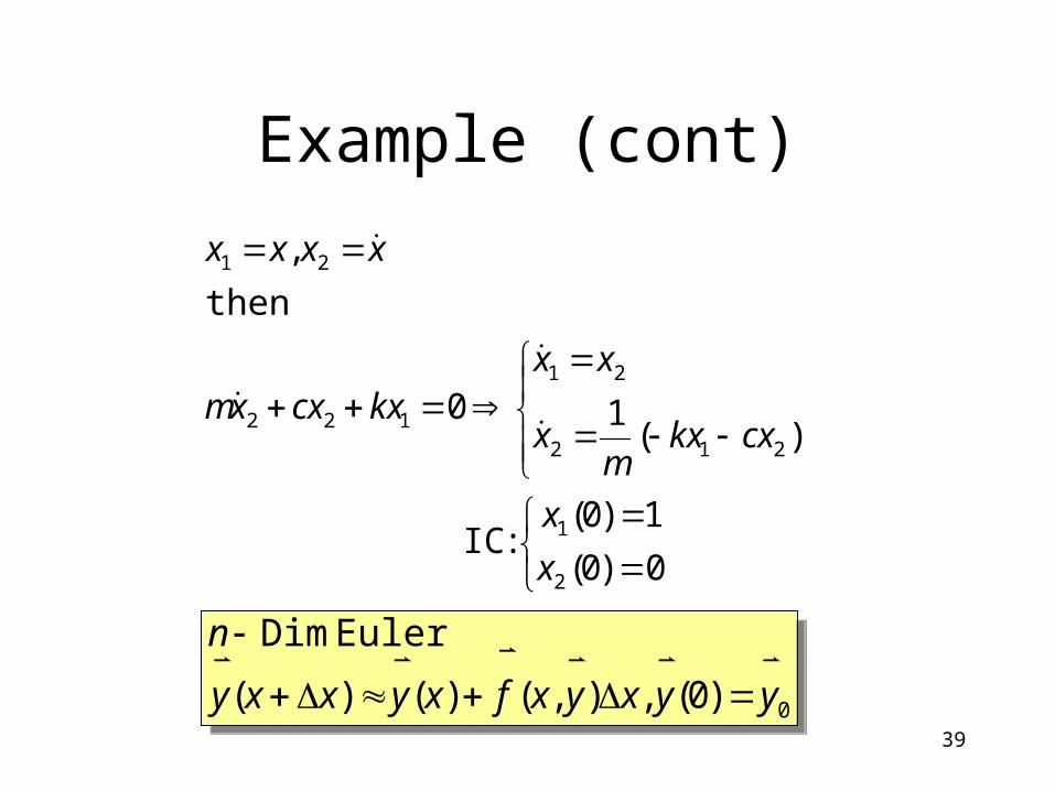
2

1

212

21

122

21

x

x

cxkxm

x

xxkxcxxm

xxxx

Example (cont)

0)0(,),()()(

Euler Dim

yyxyxfxyxxy

n

0)0(,),()()(

Euler Dim

yyxyxfxyxxy

n

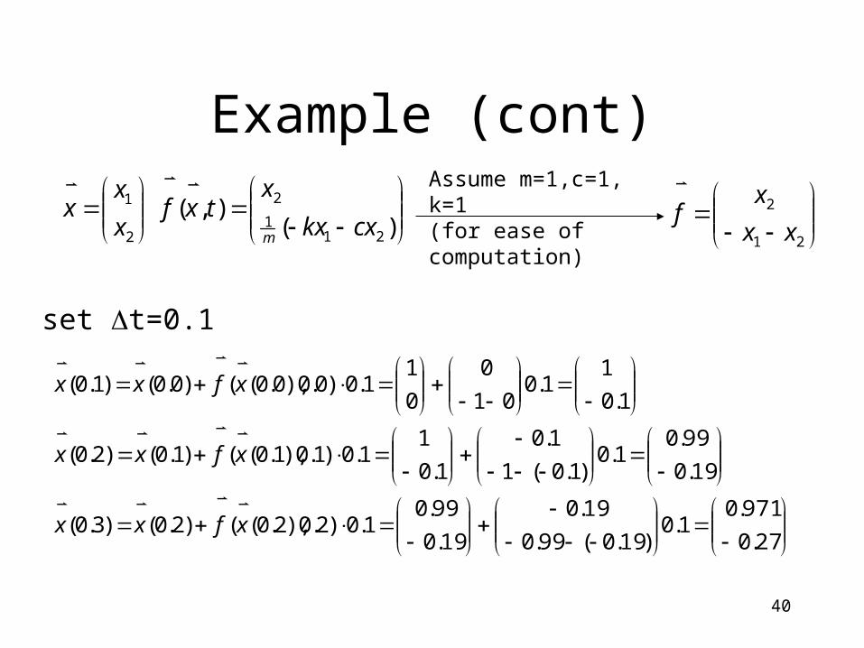
40

set t=0.1

27.0

971.01.0

)19.0(99.0

19.0

19.0

99.01.0)2.0),2.0(()2.0()3.0(

19.0

99.01.0

)1.0(1

1.0

1.0

11.0)1.0),1.0(()1.0()2.0(

1.0

11.0

01

0

0

11.0)0.0),0.0(()0.0()1.0(

xfxx

xfxx

xfxx

Example (cont)

)(),(

211

2

2

1

cxkx

xtxf

x

xx

m

Assume m=1,c=1, k=1 (for ease of computation)

21

2

xx

xf

41

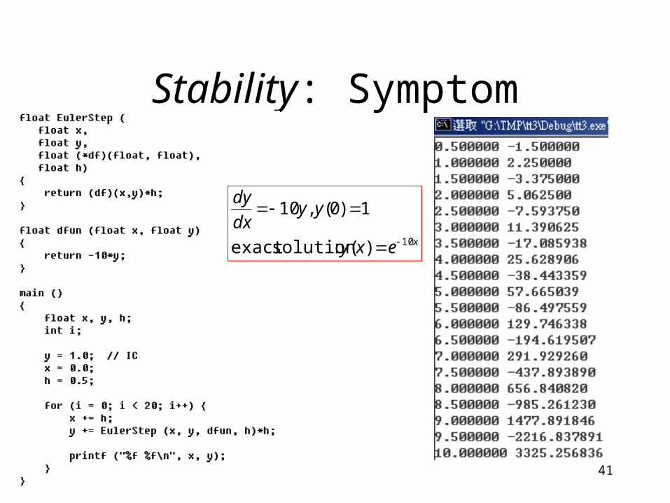
Stability: Symptom

xexy

yydx

dy

10)( :solutionexact

1)0(,10

42

Symptom: Unstable Spring System

Start with this …

Become unstable instantly …

Cause by stiff (k=4000) springsCause by stiff (k=4000) springs

43

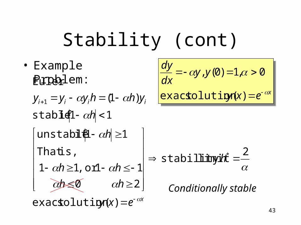
Stability (cont)• Example Problem:

xexy

yydx

dy

)( :solutionexact

0,1)0(,

xexy

yydx

dy

)( :solutionexact

0,1)0(,

Conditionally stablex

iiii

exy

h

hh

hh

h

h

yhhyyy

)( :solutionexact

2limit stability

2 0

1 1or ,1 1

is,That

11 if unstable

11 if stable

)1(

:Euler

*

1

44

Discussion

• Different algorithm different stability limit– Check Midpoint Method

• Different problem different stability limit– use the previous problem as benchmark

45

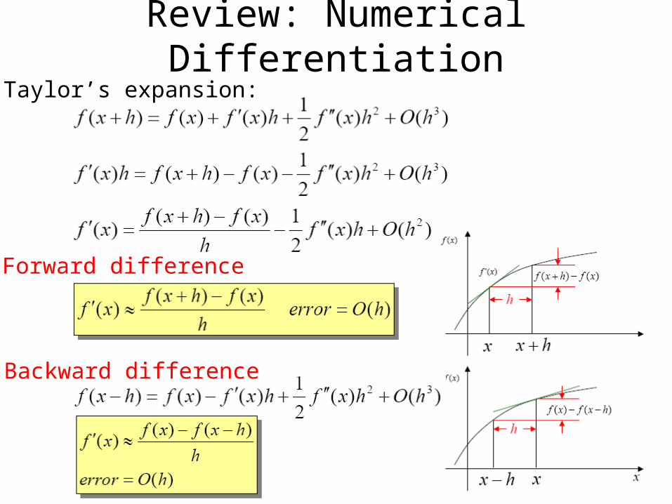
Review: Numerical DifferentiationTaylor’s expansion:

Forward difference

Backward difference

46

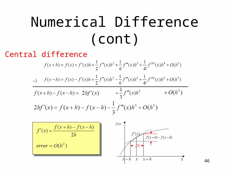
Numerical Difference (cont)

Central difference

47

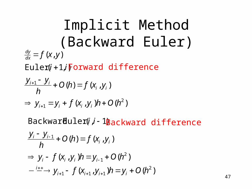
Implicit Method (Backward Euler)

)(),(

)(),(

),()(

)1,(:Euler Backward

2111

21

1

hOyhyxfy

hOyhyxfy

yxfhOh

yy

ii

iiiii

iiii

iiii

)(),(

),()(

),1( :Euler

),(

21

1

hOhyxfyy

yxfhOh

yy

ii

yxf

iiii

iiii

dxdy

Forward difference

Backward difference

48

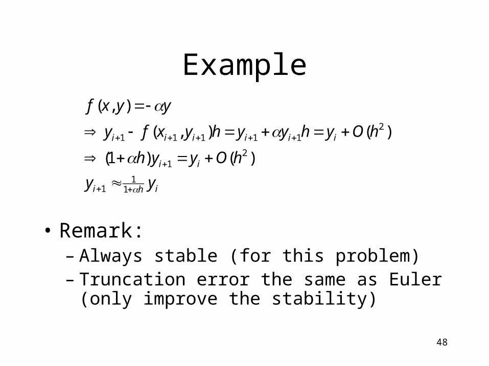
Example

• Remark:– Always stable (for this problem)– Truncation error the same as Euler (only

improve the stability)

ihi

ii

iiiiii

yy

hOyyh

hOyhyyhyxfy

yyxf

11

1

21

211111

)()1(

)(),(

),(

49

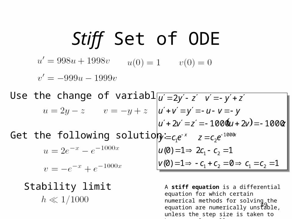
Stiff Set of ODE

Stability limit

Use the change of variable

101)0(

121)0(

1000210002

2

2121

21

100021

ccccv

ccu

eczecy

zvuzvu

yvuyvu

zyvzyu

xx

101)0(

121)0(

1000210002

2

2121

21

100021

ccccv

ccu

eczecy

zvuzvu

yvuyvu

zyvzyu

xxGet the following solution:

A stiff equation is a differential equation for which certain numerical methods for solving the equation are numerically unstable, unless the step size is taken to be extremely small

50

51

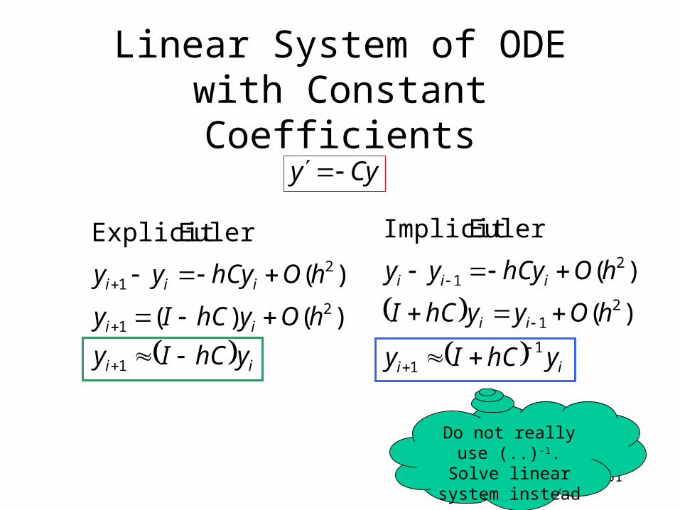
Linear System of ODE with Constant Coefficients

ii

ii

iii

yhCIy

hOyyhCI

hOhCyyy

11

21

21

)(

)(

EulerImplicit

ii

ii

iii

yhCIy

hOyhCIy

hOhCyyy

1

21

21

)()(

)(

EulerExplicit

Cyy

Do not really use (..)-

1. Solve linear system instead

52

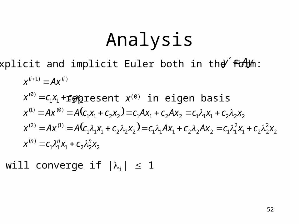
Analysis

222111)(

22221

211222111222111

)1()2(

22211122112211)0()1(

2211)0(

)()1(

xcxcx

xcxcAxcAxcxcxcAAxx

xcxcAxcAxcxcxcAAxx

xcxcx

Axx

nnn

ii

x will converge if |i| 1

represent x(0) in eigen basis

Explicit and implicit Euler both in the form: Ayy

53

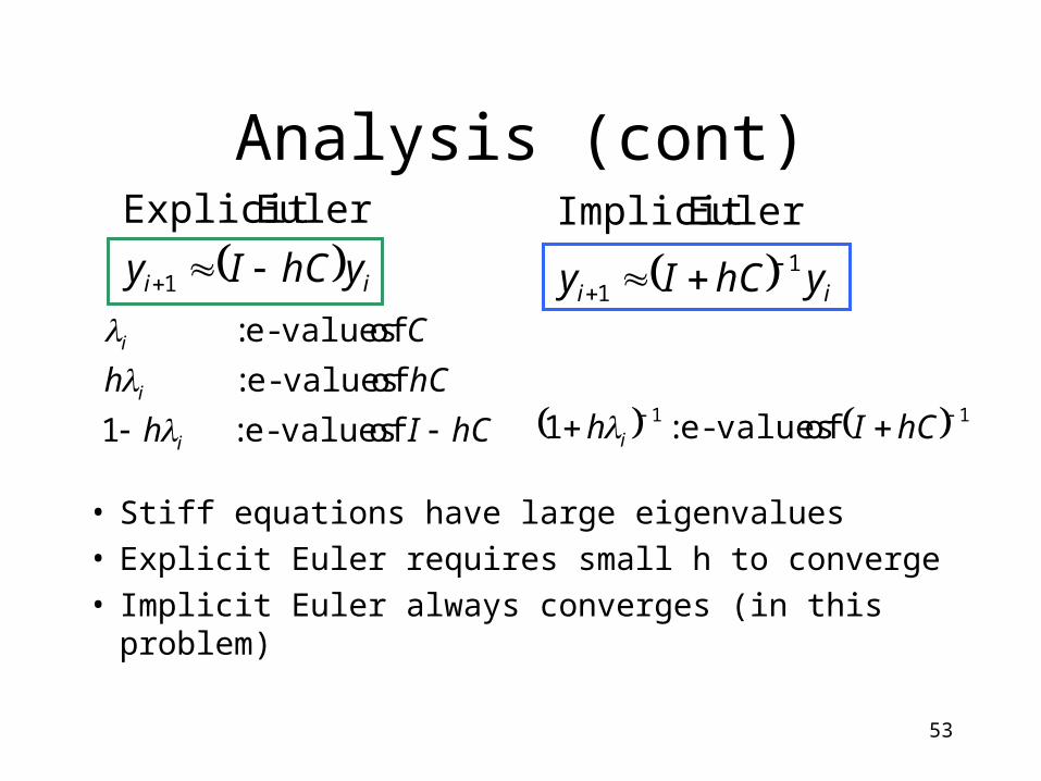
Analysis (cont)

• Stiff equations have large eigenvalues• Explicit Euler requires small h to converge• Implicit Euler always converges (in this problem)

hCIh

hCh

C

i

i

i

of values-e: 1

of values-e:

of values-e :

11 of values-e: 1 hCIh i

ii yhCIy 1

EulerExplicit

ii yhCIy 11

EulerImplicit

54

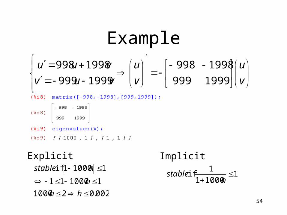
Example

v

u

v

u

vuv

vuu

1999999

1998998

1999999

1998998

Explicit

002.021000

1100011

110001 if

hh

h

hstable

Implicit

110001

1 if

hstable

55

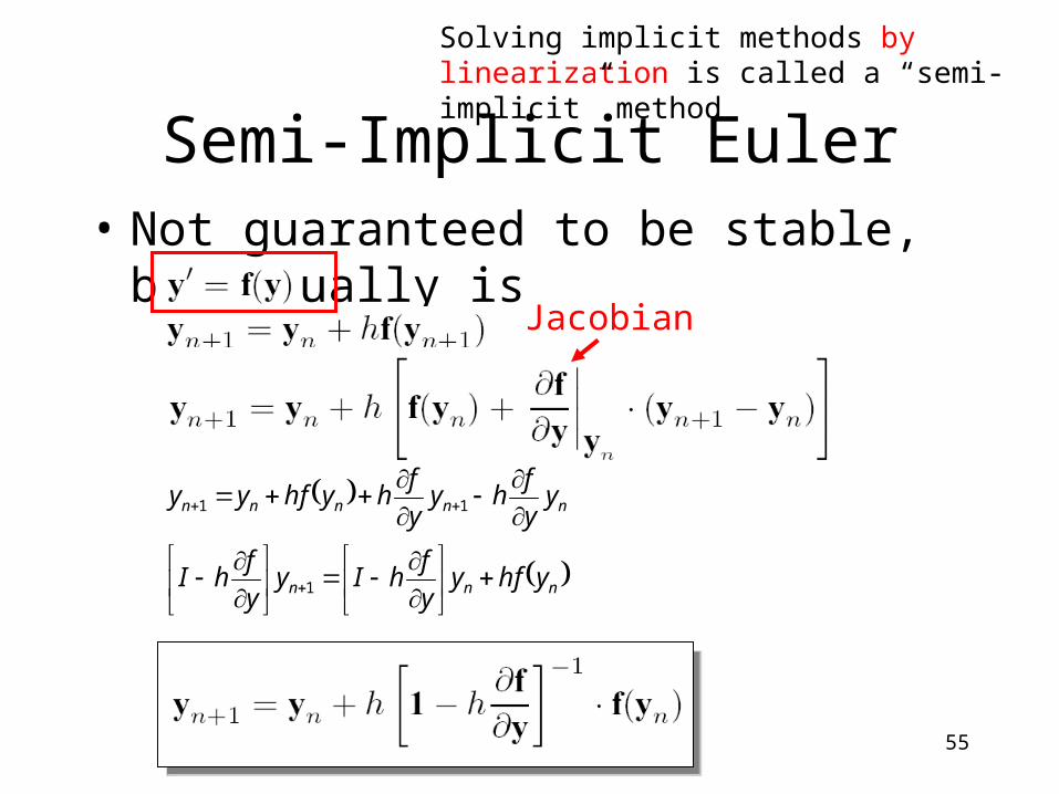
Semi-Implicit Euler• Not guaranteed to be stable, but usually is

Solving implicit methods by linearization is called a “semi-implicit” method

nnn

nnnnn

yhfyy

fhIy

y

fhI

yy

fhy

y

fhyhfyy

1

11

Jacobian

56

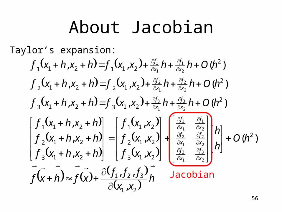
About Jacobian

h

xx

fffxfhxf

hOh

h

xxf

xxf

xxf

hxhxf

hxhxf

hxhxf

hOhhxxfhxhxf

hOhhxxfhxhxf

hOhhxxfhxhxf

xf

xf

xf

xf

xf

xf

xf

xf

xf

xf

xf

xf

21

321

2

213

212

211

213

212

211

2213213

2212212

2211211

,

,,

)(

,

,

,

,

,

,

)(,,

)(,,

)(,,

2

3

1

3

2

2

1

2

2

1

1

1

2

3

1

3

2

2

1

2

2

1

1

1

Jacobian

Taylor’s expansion:

57

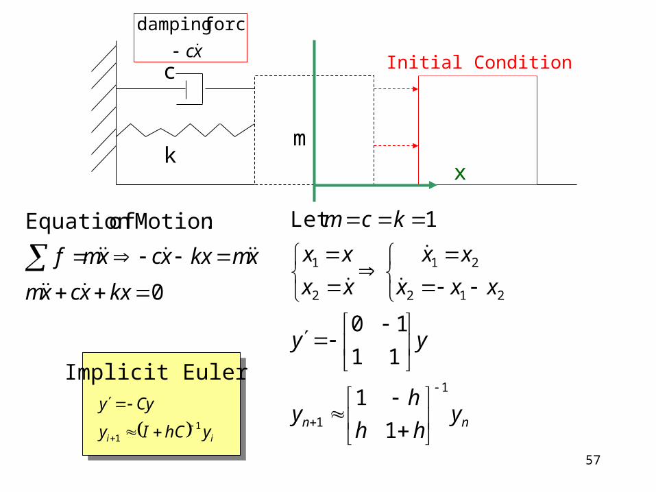
c

k

Initial Condition

x

m

0

:Motion ofEquation

kxxcxm

xmkxxcxmf

nn yhh

hy

yy

xxx

xx

xx

xx

kcm

1

1

212

21

2

1

1

1

11

10

1Let

xc

force damping

Implicit Euler

ii yhCIy

Cyy1

1

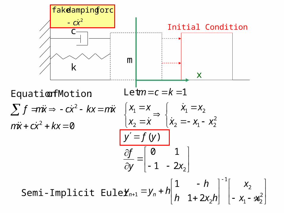
58

c

k

Initial Condition

x

m

0

:Motion ofEquation

2

2

kxxcxm

xmkxxcxmf

221

2

1

21

2

2212

21

2

1

21

1

21

10

)(

1Let

xx

x

hxh

hhyy

xy

f

yfy

xxx

xx

xx

xx

kcm

nn

2

force damping fake

xc

Semi-Implicit Euler

59

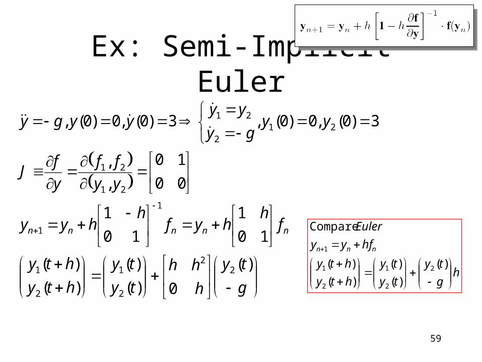
Ex: Semi-Implicit Euler

g

ty

h

hh

ty

ty

hty

hty

fh

hyfh

hyy

yy

ff

y

fJ

yygy

yyyygy

nnnnn

)(

0)(

)(

)(

)(

10

1

10

1

00

10

,

,

3)0(,0)0(,3)0(,0)0(,

22

2

1

2

1

1

1

21

21

212

21

hg

ty

ty

ty

hty

hty

hfyy

Euler

nnn

)(

)(

)(

)(

)(

Compare

2

2

1

2

1

1

60

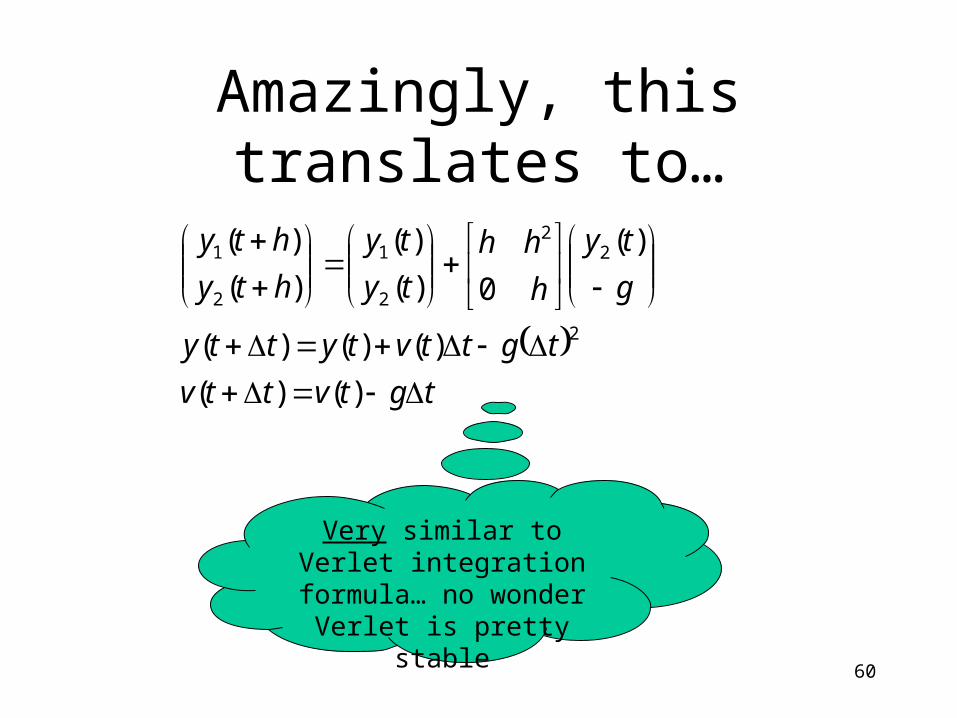
Amazingly, this translates to…

tgtvttv

tgttvtytty

g

ty

h

hh

ty

ty

hty

hty

)()(

)()()(

)(

0)(

)(

)(

)(

2

22

2

1

2

1

Very similar to Verlet integration formula… no

wonder Verlet is pretty stable

61

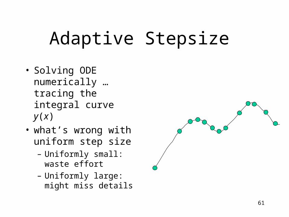
Adaptive Stepsize

• Solving ODE numerically … tracing the integral curve y(x)

• what’s wrong with uniform step size– Uniformly small:

waste effort

– Uniformly large: might miss details

62

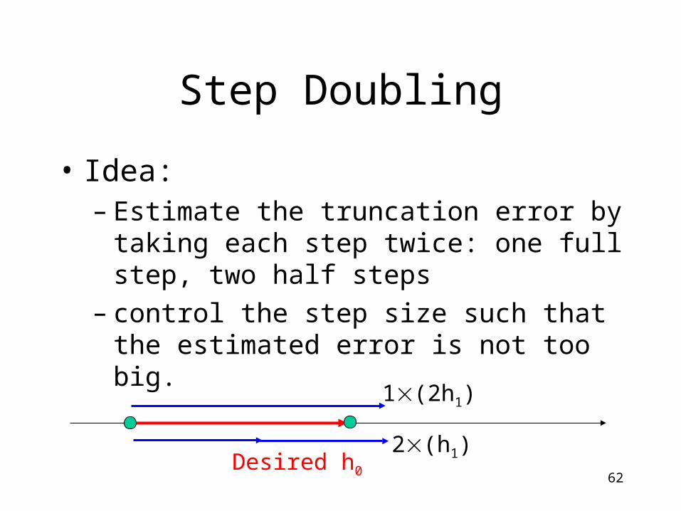
Step Doubling

• Idea:– Estimate the truncation error by taking each

step twice: one full step, two half steps– control the step size such that the estimated

error is not too big.

1(2h1)

2(h1)Desired h0

63

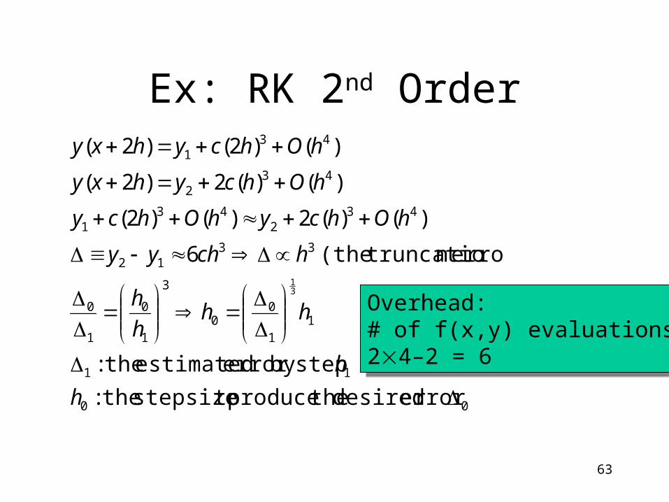
Ex: RK 2nd Order

00

11

11

00

3

1

0

1

0

3312

432

431

432

431

error desired theproduce tostepsize the:

stepby error estimated the:

error)n truncatio(the 6

)()(2)()2(

)()(2)2(

)()2()2(

31

h

h

hhh

h

hchyy

hOhcyhOhcy

hOhcyhxy

hOhcyhxy

Overhead: # of f(x,y) evaluations24–2 = 6

Overhead: # of f(x,y) evaluations24–2 = 6

64

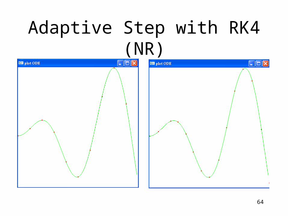
Adaptive Step with RK4 (NR)

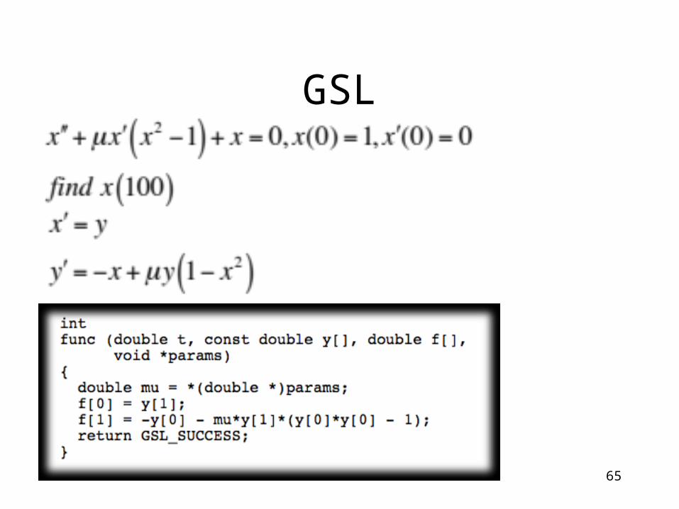
GSL

65

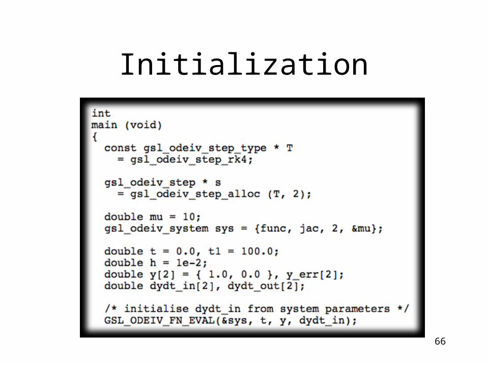
Initialization

66

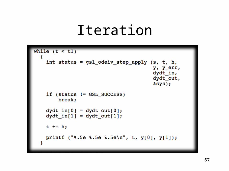
Iteration

67