1

One Size Fits All? :Computational Tradeoffs in MixedInteger Programming Software

Bob Bixby, Mary Fenelon, Zonghao Gu, Ed Rothberg, and Roland Wunderling

ILOG, Inc.

2

A MIP Code is a Bag of Tricks

Presolve Cutting planes

Gomory cuts Knapsack cuts Etc.

Node presolve Heuristics Node selection strategy Etc.

3

1. Improvement on a test set

2. Evaluation and tuning on a wider problem set

3. Implementation and deployment in a MIP code

4. Modelers (silently) benefit

Typical Path to Widespread Adoption of a New Technique

4

Cuts 53.7X Gomory 2.5X MIR 1.8X Knapsack 1.4X Flow covers 1.2X Implied bounds 1.2X …

Presolve 10.8X Heuristics 1.4X Node presolve 1.3X Probed dives 1.1X

A Few Examples[Bixby, Fenelon, Gu, Rothberg, Wunderling, 2002]

5

1. Improvement on a test set

2. Overall degradation on a wider problem set

3. Not implemented in a MIP Code

4. Modeler reads paper and implements technique

Unlikely Path to Widespread Adoption of a New Technique

6

1. Improvement on a test set

2. Overall degradation on a wider problem set

3. Implemented in a MIP code anyway

4. Modeler:1. Reads documentation or paper

2. Recognizes that technique will be effective on his models

3. Enables non-default option in MIP code

Another Unlikely Path to Widespread Adoption of a New Technique

7

Explore logical consequences of fixing binary variables to 0/1 Variable fixing Coefficient lifting Implied bound cuts

Model mod011.mps Moderately difficult model from MIPLIB set

Example : Probing[Brearley, Mitra, Williams, 1975]

8

Model mod011.mps without probing Nodes Cuts/ Node Left Objective IInf Best Integer Best Node ItCnt Gap 0 0 -6.2082e+007 16 -6.2082e+007 2254

… -5.8833e+007 48 Flowcuts: 5 6840* 52 52 0 -4.1232e+007 -5.8811e+007 12548 42.64%* 53 50 0 -5.1414e+007 -5.8811e+007 12565 14.39%* 156 114 0 -5.3439e+007 -5.8563e+007 27821 9.59%* 319 242 0 -5.3676e+007 -5.8305e+007 52401 8.62%* 955 716 0 -5.3779e+007 -5.7598e+007 180050 7.10%* 976 721 0 -5.3833e+007 -5.7545e+007 183880 6.89%* 1168 858 0 -5.3863e+007 -5.7390e+007 217373 6.55%* 1187 868 0 -5.3898e+007 -5.7388e+007 220889 6.47%* 1748 1205 0 -5.4059e+007 -5.7096e+007 331173 5.62%* 2393 1601 0 -5.4088e+007 -5.6805e+007 475812 5.02%* 2569 1395 0 -5.4422e+007 -5.6752e+007 511588 4.28%* 12152 3545 0 -5.4559e+007 -5.5205e+007 2175100 1.18%

Implied bound cuts applied: 410Flow cuts applied: 695Flow path cuts applied: 117Gomory fractional cuts applied: 14

Integer optimal solution: Objective = -5.4558535014e+007Solution time = 2572.66 sec. Iterations = 2444566 Nodes = 16437

9

Model mod011.mps with probing

Reduced MIP has 1558 rows, 6895 columns, and 14668 nonzeros.

…Probing added 286 nonzerosProbing time = 0.31 sec.

Nodes Cuts/ Node Left Objective IInf Best Integer Best Node ItCnt Gap

0 0 -5.9923e+007 16 -5.9923e+007 2165

… -5.4636e+007 33 Cuts: 10 25098* 33 33 0 -5.4195e+007 -5.4636e+007 34600 0.81%* 51 38 0 -5.4219e+007 -5.4634e+007 43147 0.77%* 78 33 0 -5.4559e+007 -5.4625e+007 57046 0.12%

Implied bound cuts applied: 2398Flow cuts applied: 496Flow path cuts applied: 207Gomory fractional cuts applied: 3

Integer optimal solution: Objective = -5.4558535014e+007Solution time = 206.73 sec. Iterations = 59222 Nodes = 110

10

Mean performance ratio:1s 0.6810s 0.59100s 0.34500s 0.311000s 0.25

Probing on a Wider Set of Models

11

Use dual simplex to choose branching variable Estimate objective degradation by performing a

limited number of simplex iterations Maximize the minimum degradation

Finding optimal solutions for large Traveling Salesman Problems Crucial for improving objective lower bound

Another Example : Strong Branching[Applegate, Bixby, Chvatal, and Cook, 1995]

12

Mean performance ratio:1s 0.9610s 0.76100s 0.72500s 0.661000s 0.69

Strong Branching on a Wider Set of Models

13

Consistency BetweenUser Goals and Code Goals

14

Emphasis before CPLEX 7.0: Minimize time to proven optimality

Important components of approach: Aggressive cut generation Search strategy that attempts to avoid

unnecessary work Depth First Search until first feasible found Best Bound Search until termination

A MIP Code Has An (Implicit) Emphasis

15

User reaction Depends heavily on user metric Common metric:

Time to first “good” feasible solution

Reevaluate the bag of tricksTime to first feasible?Time to 10% (20%?) gap?

Potential Mismatch Between Goals

16

Mean performance improvement (CPLEX 7.5):

Desired optimality gap

10% 20% 30% finite 1s 1.00 0.99 1.00 1.01 10s 1.08 1.10 1.12 1.25 100s 1.17 1.26 1.31 1.51 500s 1.08 1.05 1.24 1.50 1000s 1.27 1.40 1.47 1.46

Performance for Feasibility Emphasis

17

Simple underlying algorithmic changes Less aggressive application of cuts More time spent near leaves of search tree

Could be achieved with parameter changes

Users pleased nonetheless

Describe goals rather than understanding and choosing techniques

User Emphasis Setting:Feasibility Instead of Optimality

18

Improvements reduce the importance of emphasis:More heuristics produce feasible solutions

faster and more consistentlyProbed dives make dives more likely to

lead to good feasible solutions

User Emphasis Setting in 8.0

19

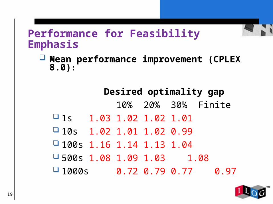
Mean performance improvement (CPLEX 8.0):

Desired optimality gap

10% 20% 30% Finite 1s 1.03 1.02 1.02 1.01 10s 1.02 1.01 1.02 0.99 100s 1.16 1.14 1.13 1.04 500s 1.08 1.09 1.03 1.08 1000s 0.72 0.79 0.77 0.97

Performance for Feasibility Emphasis

20

Test set: 978 models

Selected from our library with over 1500 models 100,000 seconds limit on ES40 Compaq Alpha Solved to optimality

775 (77%) Among those not solved to optimality

116 had gap less than 10% (11.9%)

32 had no integral solution (3.2%) MIP emphasis feasibility on the 32 models

25 found no feasible solution (2.6%)

MIP Results of CPLEX8.0[Bixby, Fenelon, Gu, Rothberg, Wunderling, 2002]

21

Natural progression:1. Try default settings

2. Specify an emphasis

3. Change parameter settings

4. Use priority order

5. Reformulate model Some models still unsolved after all these

steps

Hard Problems

22

Exploiting User Knowledge

23

Users sometimes have domain knowledge that can help solution Crucial variables Heuristics for finding good feasible solutions Strategies to decompose the problem through

branching Special cutting planes Etc.

User knowledge on the original model MIP code solves the presolved model

User Knowledge

24

MIP callbacks Cut callback Heuristic callback Branch callback Incumbent callback

Advanced presolve Allows user to express domain knowledge in

terms of the original model

Advanced Features

25

Before CPLEX 7.0 Usually need to turn off presolve (lose 10.8X) All constraints must be explicit

Since CPLEX 7.0 Can choose whether callbacks will work with

original or presolved model Can obtain mappings for variables and

constraints in the original model No need to specify all constraints up front

Lazy constraints

Adding User Cuts or Lazy Constraints

26

Original model

max {x1+x2+2x3: 3x1+3x2+4x3 6, x1, x2, x3 B}

Presolved model

max {y+2x3: 3y+4x3 6, 0 y 2, 0 x3 1, y, x3 Z}

Cut for the original model

x1 + x3 1

It cannot be transformed and added to the presolved model

Need to turn off non-linear reductions, such as parallel column reduction

Caution: User Cuts

27

Model

max {x: 5x + 3y 10, x - y 0, x 0, y 0, x Z}

x - y 0 treated as a lazy constraint

Presolve will fix y to 0 and x to 2

x – y 0 becomes 2 – 0 0

Augmented model is infeasible?

Need to turn off dual reductions Reductions that depend on the objective function

Caution: Lazy Constraints

28

Side Constraints

29

Many types of “side constraints”SOS constraintsSemi-continuous variablesCardinality constraintsMin, Max and Abs functionsLogical expressions

e.g., x = 1 implies y+z <= 3

Tour requirements (TSP)Etc.

Side Constraints

30

Example: SOS1(z1,z2) Introduce auxiliary binary variables b1, b2

z1 u1 b1; z2 u2 b2; b1 + b2 1

Pros: All MIP tricks apply (cuts, presolve, heuristics, etc.) No need to handle special cases in MIP code

Cons: Model size increases Often leads to large big-M coefficients

Handling Side Constraints - Linearize

31

Example: SOS1(z1,z2)

When both z1 > 0 and z2 > 0 at a node…

Branch on SOS1:Left child: z1 = 0

Right child: z2 = 0

Cons:Special case for each constructNo presolve, cuts, heuristics, …Looser relaxation

Handling Side Constraints - Branching

32

Is it possible to tighten relaxation without an explicit linearization?

Specialized cuts or lazy constraints E.g., cardinality constraints [de Farias and

Nemhauser], TSP [Applegate, Bixby, Chvátal, and Cook]

Need to derive for each type of non-linear constraint

Alternative: extension to Gomory cuts

Tighter Implicit Formulation?

33

Given y, xj Z+, and

y + aijxj = d = d + f, f > 0

Rounding: Where aij = aij + fj, define

t = y + (aijxj: fj f) + (aijxj: fj > f) Z Then

(fj xj: fj f) + (fj-1)xj: fj > f) = d - t Disjunction:

t d (fjxj : fj f) f

t d ((1-fj)xj: fj > f) 1-f Combining:

((fj/f)xj: fj f) + ([(1-fj)/(1-f)]xj: fj > f) 1

Gomory Cut Review

34

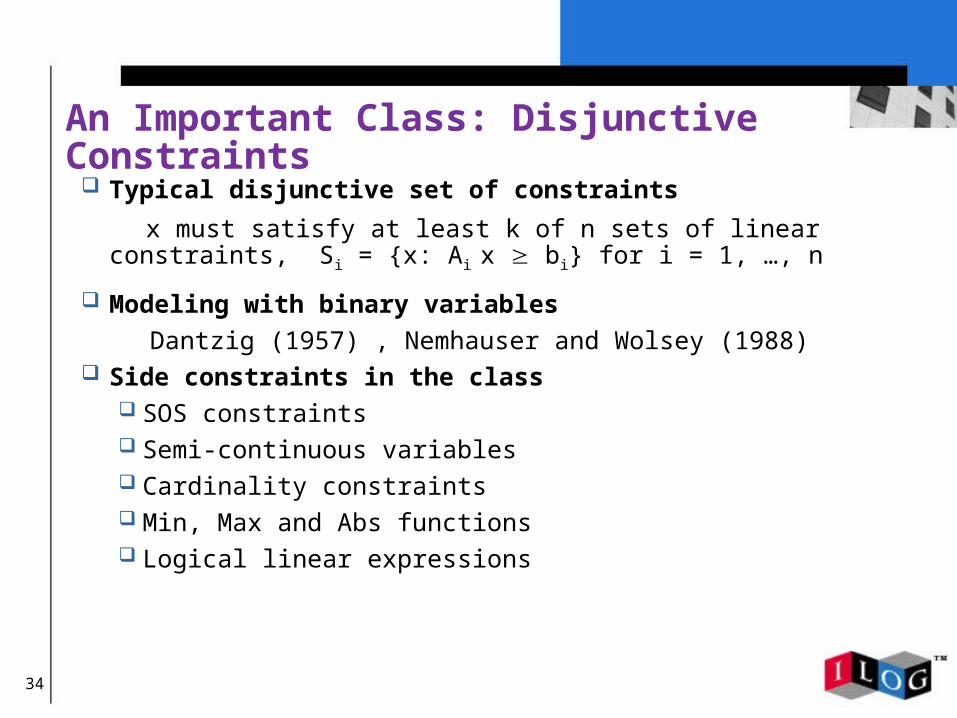
Typical disjunctive set of constraints

x must satisfy at least k of n sets of linear constraints, Si = {x: Ai x bi} for i = 1, …, n

Modeling with binary variables

Dantzig (1957) , Nemhauser and Wolsey (1988) Side constraints in the class

SOS constraints Semi-continuous variables Cardinality constraints Min, Max and Abs functions Logical linear expressions

An Important Class: Disjunctive Constraints

35

Definition

At most m variables of x1,…, xn can be positive

Use typical disjunctive set to express

Si = {x: -xi 0} for i = 1, …, n

k = n - m

Cardinality Constraint

36

Given xj R+, and

x is not in S1, S2, …, Sm, with m > n – k

Note x should be in at least k - (n - m) of the above sets

Pick a violated constraints from each set

aij xj di, i = 1, …, m

Substitute basic variables with nonbasic ones

fij xj gi, i = 1, …, m

Note gi > 0. Let hij = max (0, fij / gi), then

hij xj 1, i = 1, …, m

Combine

hij xj m + k – n

Gomory Cut Extension (with Puget)

37

Default works well to prove optimality or to find good feasible solutions for most models Try it first

CPLEX has an emphasis setting. Using it to specify a goal may help for some models

Several features are off by default Turning them on or changing parameter settings can help

solving hard models

CPLEX provides advanced routines for exploiting user knowledge They can be helpful for hard models, e.g. their use for

extending Gomory cuts for handling side constraints

One Size Fits All?