1

1 - Notes on the Stock-Flow Consistent Approach to Macroeconomic Modeling

Introduction

The aim of this paper is to present and discuss the general features of the “Stock-

Flow Consistent Approach to Macroeconomic Modeling” (SFCA, from now on).

Although the SFCA is still not widely adopted, it’s our contention that (i) it is crucial for

sound macroeconomic reasoning in general1 and, therefore, (ii) its widespread adoption

would increase both the transparency and the logical coherence of most macro models2.

In order to support our claims, we chose to divide these notes in four parts. The

first describes what exactly we mean by the “stock-flow consistent approach to

macroeconomic modeling”. As the distinguishing features of the SFC approach are

perhaps clearer when it’s contrasted to other approaches, we decided to dedicate the next

two parts of the paper to such comparisons. Therefore, the second part attempts to relate

the SFC approach to current mainstream macroeconomics, while the third (briefly) relates

it to conventional Post-Keynesian macroeconomics. The fourth and last part of this paper

attempts to summarize the “state-of-the-art” of this line of research as we see it and,

hopefully, share with the reader some of the excitement felt by SFCA authors about the

possibilities of this line of research. A couple of concluding remarks is presented in the

end of the paper.

1 The same opinion is expressed, for example, in Tobin (1980 and 1982), Godley and Cripps

(1983), Taylor (1997) and Godley and Shaikh (2002). 2 The same opinion is expressed, for example, in Lavoie and Godley (2001-02).

2

1.1 - Stock-Flow Consistent Macroeconomic Models: An Introduction

Although the 1970s marked the end of its hegemony in macroeconomics,

Keynesian thought showed vitality in that period. Indeed, in a series of seminal articles, a

distinguished group of economists at Cambridge (UK), MIT and Yale developed an

entirely new family of models very different in nature from the popular textbook version

of Keynesianism3. The 1981 Nobel Prize lecture by James Tobin – one of the main

architects of this new family of models – is perhaps the most well known and clear

exposition of the Keynesian “frontier” at that time. In the second page of that lecture,

Tobin (1982) writes that:

“Hicks’s “IS-LM” version of keynesian [theory](…) has a number of defects that have limited its

usefulness and subjected it to attack. In this lecture, I wish to describe an alternative framework, which tries

to repair some of those defects. (…). The principal features that differentiate the proposed framework from

the standard macromodel are these: (i) precison regarding time (…); (ii) tracking of stocks (…); (iii) several

assets and rates of return (…); (iv) modeling of financial and monetary policy operations (…); (v) Walras’s

Law and adding-up constraints”.

This “alternative framework” mentioned above is probably one of the best

definitions of SFCA4,5. This approach has been continuously developed in the last twenty

3 See Brainard and Tobin (1968), Tobin (1969), Foley and Sidrauski (1971), Blinder and Solow

(1973 and 1974), Foley (1975), Cripps and Godley (1976), Tobin and Buiter (1976), Turnovsky

(1977), Backus et.al. (1980), Tobin (1982), and Godley and Cripps (1983), among others. Most of

these papers aimed to address issues raised by Ott and Ott (1965) and Christ (1967, 1968). 4Even though Tobin himself didn’t call it that way. Yale people (like Fair, 1984, for example)

called it the “pitfalls approach”, in a reference to the seminal paper by Brainard and Tobin (1968).

The expression “stock-flow consistent” is commonly associated with the works of Wynne Godley

[though used also by Davis (1987a and 1987b) and Patterson and Stephenson (1988), among

others], but it seems to us that it can and should be applied more generally. Moudud (1998), for

example, preferred to use the term “Social Accounting Matrix (SAM) approach” - also widely

3

years, especially by a relatively small group of macroeconomists associated with the

Bank of England, the University of Cambridge, the Levy Economics Institute-NY, the

New School for Social Research and the University of Ottawa6, and despite its Keynesian

origins, it’s regarded as indispensable for sound macroeconomic reasoning in general7.

Most authors in this tradition would probably agree with Solow (1983, p.164) that

“perhaps the largest theoretical gap in the model of the General Theory was its relative

neglect of stock concepts, stock equilibrium and stock-flow relations. It may have been a

used by Taylor - but that doesn’t emphasize enough the crucial importance these authors give to

the coherent and explicit treatment of the inter-relationships between macroeconomic stocks and

flows at a given moment and through time. Indeed, Taylor himself (1990) provides examples of

SAMs in which only flows are taken into consideration and, therefore, the fact that a

macroeconomic model is “SAM-based” does not mean that it is “stock-flow consistent”. On the

other hand, the original version of the Godley and Cripps model (1983) is an example of a stock-

flow consistent model not presented in a SAM. The SFCA is also, clearly, a subset of what Taylor

(1997, chapter 1, p.1) calls the “structuralist approach” to macroeconomics. 5 Although the neoclassical concept of “Walras’s Law” is considered unnecessary by most SFC

authors. 6 See Rosensweig and Taylor (1984), Anyadike-Danes et al. (1987), Davis (1987a and 1987b),

Patterson and Stephenson (1988), Godley and Zezza (1989), Taylor (1990), Godley (1996, 1999a

and 1999b), Alemi and Foley (1997), Taylor (1997, 1998a, 1998b, 1999 and 2001), Moudud

(1998), Lavoie and Godley (2001-2002) and Godley and Shaikh (2002), among many others.

Godley’s intelectual debt to Tobin is explicit, for example, in Anyadike-Danes et.al. (1987) and

Godley (1996), while Taylor’s is explicit in Taylor (1990, chapter 1) and Foley’s in Foley and

Sidrauski (1971). 7 Godley and Cripps (1983, p.44), for example, argue that the SFCA is “what (…) [they] mean by

macroeconomic theory”. Taylor (1997, ch.1, p.1) expresses a similar opinion stating that

“macroeconomic frameworks which constrain sectoral and micro level social and economic

actors and their actions are the topic of (…) [macroeconomics]”. For SFC models in the tradition

of the classical economists and Marx, see Moudud (1998). Foley’s formalizations of Marx’s

4

necessary simplification for Keynes to slice the time so thin that the stock of capital

goods, for instance, can be treated as constant even while net investment is systematically

positive or negative. But those slices soon add up to a slab, across which stock

differences are perceptible. Besides, it is important to get the stock-flow relationships

right; and since flow behavior is often related to stocks, empirical models cannot be

restricted to the shortest of the short runs”8. Note, however, that explicit recognition of

stock-flow relationships – Tobin’s item (ii) above - necessarily implies a dynamic

approach to modeling and this is in sharp contrast with conventional Keynesian

economics, which generally assumes a static short run equilibrium. Indeed, in a SFC

model current flows - which are in part determined by past stocks – end up changing

(either increasing or decreasing) current stocks and, through this channel, future flows as

well9. This point is made very clearly by Tobin (1982, p.189), according to whom, “a

model of short run determination of macroeconomic activity must be regarded as

referring to a slice of time, whether thick or paper thin, and as embedded in a dynamic

process in which flows alter stocks, which in turn condition subsequent flows”.

The dynamic context necessarily implied by the explicit recognition of the stock-

flow relationships creates, by its turn, two related needs. First, one needs to be precise

circuit of capital (Foley, 1982, 1986a and 1986b) also have many elements in common with the

SFCA. 8 Tobin (1980, p.75 and 1982, p.188) and Godley (1983, p.170), at least, express essentially the

same opinion. We’ll have more to say about this issue in section 1.1.3 below. 9 As Turnovsky (1977, p.xi) puts it “[SFC] relationships necessarily impose a dynamic structure

on the macroeconomic system, even if all the underlying behavioural relationships are static”.

Turnovsky calls this SFC dynamics “the “intrinsic dynamics” of the macroeconomic system”.

5

about how one treats the passage of time – Tobin’s item (i) above. In practice, as put by

Tobin himself (1982, p.189) most SFC models:

“(…) count time in discrete periods of equal finite length. Within any period each variable assumes one and

only one value. (…). From one period to the next asset stocks jump by finite amounts. Therefore, the

demands and supplies for these jumps affect asset prices and other variables within the period, the more so

the greater the length of the period. They will also, of course, influence the solutions in subsequent

periods”.

Of course, nothing prevents one from using the same strategy with continuous time,

instead of with discrete time, but as Tobin (idem)10 reminds us:

“Either representation of time in economic dynamics is an unrealistic abstraction. We know by common

observation that some variables, notably prices in organized markets, move virtually continuously. Others

remain fixed for periods of varying length. Some decisions by economic agents are reconsidered daily or

hourly, while others are reviewed at intervals of a year or longer except when extraordinary events compel

revisions. It would be desirable in principle to allow for differences among variables in frequencies of

change and even to make those frequencies endogenous. But at present models of such realism seem

beyond the power of our analytic tools. Moreover, many statistical data are available only for arbitrary

finite periods”.

The second need, related to the first, is the need for what Wynne Godley calls an

accounting framework “with no ‘black holes’ – [in which] every flow comes from

somewhere and goes somewhere” (Godley, 1996, p.7)11. Indeed, if we want to track the

process of change of stocks by flows and the feedback of the new stocks in future flows,

we have to make sure that current stocks are exactly the result of past flow decisions. If

we don’t do that, we literally have no idea of what determined current stocks and, as a

10 Foley (1975) expresses a similar opinion as we’ll discuss in more detail below. 11 The treatment of time and the appropriate accounting are related because often the second is

determined by the first.

6

result, we can’t say that we are modeling “the process of change of stocks by flows” in an

adequate way. The “national accounting issue” is, therefore, unavoidable to the SFCA.

In these days of neoclassical hegemony it is probably important to stress right

from the start, however, that national accounting schemes are based on a pre-conceived

view about the “economically relevant sets of people and institutions (…) [within an

economy] (Taylor, 1990, p.3). As Godley (1996, p.3) puts it, “it is a matter of

ascertainable fact that the real world is characterized by a huge and complex structure of

interdependent institutions such as governments, firms, banks and households. I do not

accept that these institutions are “veils” with nothing more to do than passively sponsor

or facilitate the optimizing aspirations of individual agents; and wish, rather, to start from

a conceptual framework which has cognisance of (something remotely approaching) the

real world as we know it”12. Taylor (1997, p.1) expresses the same opinion as follows:

“(…) social accounts and social relations frame macroeconomics. The social accounts are

a skeleton, and social relations change its position over real, historical time. Specifying

just which relations drive the motions is not a trivial task (…). But the objects that move

– the observable phenomena in macro – are mostly the numbers comprising the national

income and product accounts (or NIPA) and allied systems”.

Of course, a huge number of theoretical and applied macroeconomic models –

probably beginning with Quesnay’s famous “Tableau Economique” – were phrased as (or

12 It is conceivable, however, to think about a SFC model based on several representative agents

(like a representative household, a representative bank, a representative non-financial firm and so

forth). In general, however, SFCA authors don’t use representative agents. Tobin (1989, p.18) is

probably expressing the view of most SFCA authors when he remarks that “why this

“representative agent” assumption is less ad hoc and more defensible simplification than (…)

constructs of early macro modelers (…) is beyond me”.

7

were based on) some kind of (implicit or explicit) “social accounting matrix” (or SAM13)

and, therefore, one must emphasize the importance of the “allied systems” mentioned

above by Taylor. Indeed, most of these models are based on some sort of “flow

accounting” (like the NIPA) and, therefore, either focus only on flows or deal with stocks

and flows inconsistently. Although for many applications references to stocks and/or the

bias introduced by “stock-flow inconsistency” may not be relevant, SFCA authors

strongly believe that for most kinds of macroeconomic analysis it is. SFC models

(applied or theoretical), therefore, are necessarily based on sophisticated accounting

frameworks that consistently integrate flows of income and product with flows of

financial funds and a full set of balance sheets14. To put it briefly, the adjectives “SAM-

based” and “SFC” are not synonyms, although many “SAM-based” models are indeed

SFC15.

13 Taylor (1990, p.7) traces the concept of SAMs back to Stone, R (1966), “The Social Accounts

from a Consumer Point of View”, Review of Income and Wealth, series 12, n.1. Although

Stone’s rigorous concept must be differentiated from the more generic idea that a SAM is any

kind of matrix portraying any kind of social accounting (like, for example, Quesnay’s Tableau

Economique”), the literature not always does that. Here we’ll use the generic meaning of the

term. 14 In applied work this is achieved (or approximated) through the (non-trivial) integration of

NIPA accounts with Flow of Funds accounts. The relevance of this integration has been

increasingly emphasized by the United Nation’s “System of National Accounts” as well. Dawson

(1996) is a good source for both the details of this integration and the intellectual history of the

Flow of Funds Accounts. As Dawson makes clear, FoF authors are, in many aspects, intellectual

ancestors of the SFCA approach. 15 “SAM-based” (Computable General Equilibrium) models, in Stone’s sense (see footnote 15),

are widely used in the development literature, both by orthodox and non-orthodox economists.

Taylor (1990) and Alarcón et.al. (1991), two surveys of this “SAM-based” development

8

It’ also true that a huge number of theoretical and applied macroeconomic models

discuss some sort(s) of stock-flow relation(s)16. Harrod’s famous analysis of a growing

economy and all the literature that followed it is one of the examples that quickly come to

mind. Harrod’s case is important in our argument for two reasons. First, because he was

one of the first to point out the need for intrinsically dynamic analyses of the kind

proposed by the SFCA17. Second, because even though his model explicitly theorizes

about stock-flow ratios it is not SFC, in the sense that not all macroeconomic stocks and

flows implicit in its hypotheses are accounted for. Who finances investment in Harrod’s

model? Given that savings are non-negative, wealth is certainly being accumulated, but

where’s the stock of wealth in Harrod’s model? This list could go on. In other words, a

model may very well say something about some stock-flow relation(s) without being

SFC18. And, again, even though the bias introduced by stock-flow inconsistency may be

of little relevance for the fundamental message of many macroeconomic models (as

argued by Moudud, 1998 and subsequent papers, in the case of Harrod), this has to be

proved rather than simply asserted.

literature, present many SFC and non-SFC models. Rosensweig and Taylor (1984) is often cited

as a pioneer “SAM-based” SFC model. 16The same is true, by the way, for microeconomic models. Obvious examples are models of real

estate markets and commodities in general. 17 As he put it “it is necessary to think dynamically (…) once the mind is accustomed to thinking

in terms of trends of increase, the old static formulation of problems seems stale, flat and

unprofitable” (Harrod, 1939, p.16). 18A survey of all the authors that have theorized about specific stock-flow ratios or relations

without presenting a formal SFC model would be a very large one, though, well beyond the scope

of this paper.

9

In practice, most SFC macro models follow conventional national accounts and

assume that the economy can be adequately depicted as consisting of 5 sectors, which are

(aggregations of) (i) Households, (ii) Non-Financial Firms, (iii) Financial Sector (Banks),

(iv) Government and (v) Rest of the World19,20. Of course, further aggregation or

disaggregation of some sectors and/or the elimination of a few others are possible and, in

fact, desirable depending on the nature of the analysis and the aesthetic judgement of the

model-builder. It is our contention, however, that the choice of the appropriate (SFC)

accounting structure is far from obvious and can be seen as the first fundamental

hypothesis of a SFC model. Indeed, this choice implies a huge number of non-trivial

theoretical assumptions (explicit or not) about the “players in the game and the moves

they make” (Cohen, 1986, p.3) and perhaps the best way to see it is as something

equivalent to the creation of a simple “artificial economy”21. As a consequence, different

people will have different opinions concerning the optimum size/degree of disaggregation

of the accounting structure22 and what exactly must be accounted for23.

19Making the models especially appropriate for the discussion of items (iii) and (iv) of Tobin’s

passage mentioned above. 20 The main exceptions are recent models (see, Godley, 1999b or Taylor, 1999, for examples) of

“two interdependent economies which together make up a whole world” (Godley, 1999b, p.1) 21 Note that, as Brainard and Tobin (1968, p.99) remind us, “[this procedure] guarantees us an

Olympian knowledge of the true structure that is generating the observations. (…). [But it] (…)

cannot tell us anything about the real world. You can’t get something for nothing. We realize

further that the lessons derived or illustrated by simulations of our particular structure will not be

very convincing or even interesting to people who believe that the model bears no resemblance to

the process which generate actual statistical data”. 22Given that, as put by Taylor (1990, p.1) “any economy is a maze of structural detail – more than

one could ever build into equations or use in policy design”, the choice of what to include and

what to leave out of a macroeconomic model is more an art than a science.

10

Second, we should not forget that even if we agree on the level of aggregation of

the accounting structure and on what it must account for, the facts remain that (i) the

choice of the accounting conventions is basically theory determined24 and (ii) even within

the boundaries of a given theory, in general there’s a lot of room for discretion25. This last

point is clearly put by Wynne Godley and Francis Cripps in the first paragraph of the first

chapter of their seminal book (1983, p.23): “definitions of national income, expenditure

and output, although generally chosen to make it as easy as possible to reach conclusions

about major objectives of macroeconomic policy, are in last resort arbitrary”. As a

consequence, different authors would very likely disagree not only on what to account

for, but also on the level of aggregation of the accounts and on how to account for what

they think is right to account for26.

Given all these degrees of freedom one might very well ask why someone would

bother to use any national accounting framework or data whatsoever. There are several

23Perhaps the clearest example of this fact is the distinction between the “neoclassical” accounting

of, for example, Buiter (1983) - that emphasizes future (fundamentally uncertain) revenues of

agents (like, for example, government’s future tax revenue) - and the ones in, for example,

Godley (1996) and Taylor (1997) that don’t even mention them. 24See Shaikh and Tonak (1994) for a thorough discussion about theoretical determinants of NIPA

accounting conventions. 25There is no terribly compelling reason, say, to consider consumption goods (like pens, or a pair

of jeans) that last longer than a year to be an “investment” by households as it is the current

practice in the U.S Flow of Funds accounts. NIPA accounts, for example, treat them as

consumption. 26 This, by the way, helps to explain why it is almost impossible to find any two different SFCA

authors that use the same accounting framework/conventions. Of course, papers with different

goals would probably use different accounting structures but this doesn’t explain all the

differences one finds in the accounting of SFC authors.

11

(mutually compatible) arguments for the use of models explicitly based on such things,

though. One of them, at the same time simple and compelling, is provided by Buiter

(1990, p.2), according to whom “without measurement there can be no science. Also, the

way we measure things, organize data and try to map them into their theoretical

counterparts will color our understanding of the processes we are monitoring”. A second

one, perhaps more pragmatic and probably implicit in Taylor’s views mentioned above, is

that - despite all their possible problems - national accounts of a specific type have been

made available to the public for more than 50 years now and are, certainly, the most

comprehensive set of data available about any national economy. Most economists,

whatever their persuasion, agree that not to take advantage of such an amount of data

would not make sense, although many (like Buiter, 1983 or Shaikh and Tonak, 1994)

would argue in favor of the use of modified national accounts’ data.

A third argument – Tobin’s item (v) above, first pointed out by Brainard and

Tobin (1968) and especially emphasized in the work of Wynne Godley - is that the use of

consistent accounting frameworks constrains what can be said to happen with the

economy they portray27. As Godley and Cripps (1983, p.18) eloquently put it, “the fact

that money stocks and flows must satisfy accounting identities in individual budgets and

in the economy as a whole provides a fundamental law of macroeconomics analogous to

the principle of conservation in physics”28. The fact that these constraints can be

presented in a concise and intuitive manner in SAMs explains why the SFC literature

27 See, for example, Godley and Shaikh (2002) and Taylor (1999) for details. 28 Fair (1984, p.35) also makes this point, although with considerably less enthusiasm. After

emphasizing that a macro model should try to incorporate as good micro foundations as possible

12

since Tobin (see, for example, Bakus et.al., 1980) has increasingly used these matrices to

summarize the accounting framework of macroeconomic models.

Fourth, accounting frameworks provide “skeletons” (Taylor, 1997, p.1) that

“come to life as (...) economic model(s)” (Backus et.al., p. 262) when behavioral

assumptions are added to the accounting framework. As put by Taylor (1991, p.41), the

accounting serves as a basis to the definition of ““closures” of a (…) macro model, to

adopt a methodology from Sen (1963) and a term from Taylor and Lysy (1979).

Formally, prescribing a closure boils down to stating which variables are endogenous or

exogenous in an equation system largely based upon macroeconomic accounting

identities, and figuring out how they influence one another”. As stressed by Taylor (1990,

1991 and 1997), it’s often possible to phrase the views of different authors as different

“closures” for the same accounting framework. Note, however, that different authors are

likely to disagree also on the choice of the appropriate “skeleton” itself and therefore this

procedure may imply a significant bias – a kind of “home court advantage” for some

views over the others.

1.2 - The SFCA and mainstream macroeconomics

The first thing we need to do in order to relate the SFCA to mainstream

macroeconomics is to define the later. This is not an easy task, though. As Fair (2000,

p.2) reminds us, “at least since Lucas’s (1976) critique of macroeconometric models,

[mainstream] macroeconomics has been is a state of flux. Beginning in the 1970's,

and account for the possibility of disequilibrium, he adds that a model should also (“somewhat

less importantly”) “account explicitly for balance sheet and flow of funds constraints”.

13

macroeconomic research scattered in a number of directions and many puzzled as to

whether the field is going anywhere".

So, rather than trying to accomplish the huge task of surveying all mainstream

lines of research in macroeconomics, we’ll try here to paint a general (and impressionist)

picture of “mainstream macro” based on a few, widely accepted, mainstream

methodological beliefs and families of models and then compare it to the SFCA. This is

what we’ll do in what follows.

1.2.1 - Parables and all that

As James Tobin aptly noted more than a decade ago:

“In journals, seminars, conferences and classrooms macroeconomic discussion has become a babble of

parables. The parables are often specific to one stylized fact, for example the correlation of nominal prices

and real output in cyclical fluctuations. Their usual inability to fit other stylized facts appears not to bother

the authors of papers of this genre. The parables always rely on individual optimization, across time and

states of nature. They differ in the arbitrary institutional restrictions they specify on technology, markets, or

information” (Tobin, 1989, p. 19)

Indeed, one of the distinguishing features of today’s mainstream macroeconomics

is that it doesn’t care at all to build models that look like “the real world as we know it”.

On the contrary, it seems that the predominant view among mainstream economists is

that “any model that is well enough articulated to give clear answers to the questions we

put to it will necessarily be artificial, abstract and patently unreal” (Lucas, 1980, quoted

in Hoover, 2001, p.139) and, therefore, ““insistence on the realism” of an economic

model subverts its potential usefulness in thinking about reality” (Hoover, 2001, p.139).

As a result, mainstream discourse about classic macroeconomic issues is now spread

14

among different branches of the profession (i.e, labor, development, monetary,

international and public economics) besides macroeconomics proper, each of which using

their own set of nice optimizing “parables” to explain reality either directly or with the

help of very simplified macroeconomic models.

As it should be clear from the previous section, this trend goes against the SFCA

view. One of the main goals SFC model builders seek to achieve is to capture the

“essential interdependences” (Brainard and Tobin, 1968, p.99) between (real)

macroeconomic sectors, a feature of reality considered too important to be “simplified

away” from the analysis. This potential advantage, however, doesn’t come without a cost

because a more detailed approach implies an increase in the complexity of the relevant

model. On the other hand, it’s undeniable that in actual economies each macroeconomic

sector interacts with all the others in many different and complex ways. Bonds issued by

the government, for example, are held and traded by firms, banks, households and

possibly also by the rest of the world, often in many differentiated markets; goods

produced by firms are also bought by all the other macroeconomic sectors as well; banks

provide loans to many other macroeconomic sectors; and the list goes on. It is also true

that a given financial asset is often issued by several different macroeconomic sectors.

For example, banks, firms and the rest of world can all issue equity, all these sectors and

the government can issue bonds, etc. In other words, each actual sectoral balance sheet

consist of a very large number of assets (which are also liabilities of other sectors) and

liabilities (which are also assets of other sectors).

As a consequence, as put by Godley and Zezza (1989, p.3), “the simplest realistic

[SFC] model requires a relatively large number of accounting equations”. Most SFCA

15

authors deal with this problem by imposing simplifying assumptions to the accounting

structure like, say, “only domestic firms issue equity”, or “only banks buy bonds from the

rest of the world” and, while it’s true that in many real economies some holdings of

assets by sectors can indeed be neglected, the choice of simplifying assumptions is bound

to be controversial. As put by Taylor (1990, p.4) “the degrees of freedom available to any

actor depend on institutions and history of the economy at hand; incorporating them in a

convincing fashion is part of the model-building art”29. The bottom line is that, although

29The issue at hand is somewhat analogous to the specification problem in econometrics. We can

either underestimate or overestimate the importance of sectoral interdependence (by analogy to

underparametrize/overparametrize a regression). In the first case, we’ll probably get biased

results in the sense that our model fails to capture “essential interdependences” between sectors

and, therefore, gives us a distorted picture of reality. In the second case we lose precision, in the

sense that the relevant causal mechanisms are obscured by the irrelevant ones. In order to fully

understand what is involved in “over-aggregating” a SFC model, one has to (i) have in mind that

sectoral accounts are obtained by simply adding up the individual accounts of the members of the

sector; and (ii) note that by following this procedure one loses trace of all “intra-sectoral”

transactions. If, for example, a bank repays a loan to another bank, this transaction will not appear

in the accounts of the banking sector as a whole (since the payment of one bank will cancel out

with the receipt of the other). The fact that these transactions are neglected in SFC macromodels

is not supposed to mean, of course, that they are not relevant per se, but that they are not crucial

to the understanding of the behavior of the economy “as a whole”. The risk of working with an

“over-aggregated” model is therefore to neglect differences among “sub-sectors” which are

indeed important to the understanding of the economy as a whole. Note also that “over-

aggregation” is not the only possible form of “under-parametrization” Another important kind is

the omission of relevant kinds of transactions among sectors. If, for example, the households’

sector is responsible for a significative part of the aggregate demand for, say, bank loans, it’s

clear that an assumption like “households don’t have access to credit” will add a bias to the

model. The case of “overparametrization” is somewhat easier to analyze. No qualitative detail is

likely to be added if we disaggregate the households in, say, “basketball lovers”, “football lovers”

or “neutral”, but the increased number of equations/variables in the model will certainly make the

16

SFCA authors have no problems acknowledging the trivial fact that all models are

unrealistic in some degree, ceteris paribus they prefer more realism to less.

1.2.2 - Isn’t the current mainstream SFC, after all?

The mainstream emphasis on unrealistic parables is not enough to characterize it

as stock-flow inconsistent. The very fact that SFC requirements are not even mentioned

by most mainstream practitioners implies they are considered either trivial or irrelevant.

It might, indeed, be the case that, as unrealistic as they are, mainstream models would

perform well in all Tobin’s five items above. In order to address these issues we must dig

a little deeper and that’s what we’ll do in what follows. Of course, as both the number of

neoclassical parables available in the market and the number of possible mainstream

macroeconomic models based on these parables (or combinations of these parables) are

very big, we’ll have to deal here only with the ones we deem more important and/or

popular.

We shall begin with the most rigorous neoclassical model, i.e, Arrow-Debreu’s

general equilibrium model with perfect markets for all present and contingent

commodities. This model is relevant not only because of its intellectual prestige, but

because “in this situation each individual knows all future prices in all contingencies, and

these future prices actually occur. Each firm or household can choose a path for

investment or consumption, and the choice of path simultaneously implies a portfolio of

analysis of its properties more difficult. Indeed, given that it’s often impossible to find analytic

solutions even for relatively simple systems of difference/differential equations, the comparative

statics/dynamics properties of most SFC models can only be studied by means of repeated

computer simulations, a procedure that gets more complicated as models grow in size.

17

assets at each instant. Under these strong hypotheses there is no need to distinguish (…)

between stock decisions and flow decisions, because they are always mutually

consistent” (Foley and Sidrauski, 1971, p.4). So, assuming a competent auctioneer, we

can be sure that flows increase/decrease stocks exactly as they must. The problem here,

as is well known, is that this model has clear problems with at least two features of

Tobin’s definition, i.e, the “careful treatment of time” (since it’s static) and the explicit

“modeling of monetary operations” (because it has no obvious place for money).

This difficulty in dealing with money is also present in the mainstream

workhorses, i.e, the Ramsey and OLG models30. This is not to say that money cannot be

included in these models, but that this inclusion is somewhat artificial. One way to do it –

that brings the models closer to the SFC paradigm – is through the introduction of the so-

called “Clower constraint condition” (or “cash in advance” constraint), i.e, the fact that

“money buys goods and goods buy money but goods do not buy goods” (Blanchard and

Fischer, 1989, p.165)31. A good example of such models is David Romer’s OLG-Cash in

advance model (idem, p.165-180), which does get reasonably good grades in many of

Tobin’s items, even if one considers that it simplifies things a little too much assuming

that the government creates money by giving it to newborn babies “as transfers” (even

though there are banks in the model!). This problem isn’t that important, though, since

Romer’s model could conceivably be adapted to provide a better treatment of “financial

30 See, for example, the textbook expositions of Blanchard and Fischer (1989, ch.4) and Romer

(1996,ch.2). 31 Another is the inclusion of money in the utility function of agents. The Clower constraint is

somewhat problematic because credit also buys goods. The “money in the utility function”

hypothesis is problematic because people in general derive utility from goods not from painted

pieces of paper. See Blanchard and Fischer (1989, ch.4) for a discussion.

18

and monetary operations” and improve its SFC grade32. What is relevant to our point –

and will be further discussed in the next section - is that, even though it’s possible to

make most mainstream models SFC, most mainstream macroeconomists simply don’t

care to do it.

Before discussing some possible reasons for this last fact, it must be mentioned

that despite all their academic predominance, the mainstream “workhorses” are rarely, if

at all, used in practice by applied macroeconomists. As put by John Taylor (2000, p. 90,

quoted in Fair, 2000, p.2), “at the practical level, a [new] common view of

macroeconomics is now pervasive in policy-research projects at universities and central

banks around the world.” According to Fair (2000, p.3) this view, summarized in Clarida,

Galí, and Gertler (1999), is based on three basic equations, which are: (i) an “interest rate

rule: The Fed adjusts the real interest rate in response to inflation and the output gap

(deviation of output from potential)33. The real interest rate depends positively on

inflation and the output gap. Put another way, the nominal interest rate depends positively

on inflation and the output gap, where the coefficient on inflation is greater than one”; (ii)

a “price equation: Inflation depends on the output gap, cost shocks, and expected future

inflation”; and (iii) an “aggregate demand equation: aggregate demand (real) depends on

the real interest rate, expected future demand, and exogenous shocks. The real interest

32 As Blanchard and Fischer (1989, p.179) put it, the model “gives a flavor of the complexity of

money flows in an actual economy”. SFCA authors expect models to do much better than that,

though. 33 As put by Blinder (1998, p.27-28) “ferocious instabilities in estimated LM curves in the U.S,

U.K, and many other countries, beginning in the seventies and continuing to the present day, led

economists and policy makers alike to conclude that money-supply targeting is simply not a

19

rate effect is negative. In empirical work the lagged interest rate is often included as an

explanatory variable in the interest rate rule. This picks up possible interest rate

smoothing behavior of the Fed” (Fair, 2000, p.2-3).

Although the model described above looks pretty much like a conventional

AD/AS model with endogenous money, the authors take great pride in the fact that these

equations are based on a general equilibrium model with optimizing representative

agents. For us what is important to note is that - like its distant cousin, the old IS/LM

equilibrium - the “new consensus” leaves aside important stock-flow relations34. As Fair

(2000, p.28-29) points out, this view is “unrealistically simple”, among other things

because “all stock effects are omitted” (including wealth effects) as well as the “interest

income effect” that arises from the undisputed fact that “households hold a large amount

of short term securities of firms and the government, and when short term interest rates

change, the interest revenue of households changes”.

We finish this quick (and partial) survey of current mainstream macroeconomic

models based on “rigorous microfoundations”, reminding the reader that a “a variety of

ad-hoc models have played, and continue to play, important roles in influencing the way

[mainstream] economists, and perhaps more importantly, policy-makers, think about the

role of monetary policy (Walsh, 1998, p.3)35. The same point is made by Krugman (2000,

p.42), according to whom “(…)microfounded models have not lived up to their promise”

(in the particular sense that they didn’t add “noticeably to our ability to match the

viable option. (…) As Gerry Bouey, a former governor of the Bank of Canada put it: we didn’t

abandon the monetary aggregates, they abandoned us”. 34 For details about the “New Consensus view”, see Taylor, J.B (2000), Clarida, Gali and Gertler

(1999) and Fair (2000).

20

phenomena”, ibid, p.39) and, therefore, “after 25 years of rational expectations,

equilibrium business cycles, growth and new growth, and so on, when the talk turns to

the next move by the Fed, the European Central bank, or the Bank of Japan, when one

tries to see a away out of Argentina’s dilemma, or ask why Brazil’s devaluation turned

out relatively well, one almost inevitably turns to the sort of old-fashioned (…) [IS-LM]

model macro (…)”.

1.2.3 - Why should one care about SFC issues? A mainstream perspective

Considering that many neoclassical authors stressed the importance of SFC issues

in the sixties and seventies36, the careless approach of current mainstream concerning

these issues may strike some as surprising. Foley (1975), however, offers an elegant

explanation of this apparent paradox. Indeed, well before the “rational expectations”

hypothesis became hegemonic in the mainstream, Foley proved that, under the

assumption of “perfect foresight on average”37, the distinction between stock and flow

equilibria in asset markets is non-existent. In other words, under the assumption of

rational expectations there’s no logical problem in phrasing macroeconomic models just

in terms of flows (or stocks), since a flow (stock) equilibrium would necessarily imply a

35 For a detailed account of central banking in practice, see Blinder (1998). 36 See, for example, Christ (1967, 1968), Foley and Sidrauski (1971), Foley (1975), Turnovsky

(1977) and Buiter (1980, 1983). 37 Foley uses the term “perfect foresight” without the qualification “on average”, but explains that

“in more complex models of where expectations are represented as probability distributions, (…)

[my] notion of “perfect foresight” corresponds to the assumption that the mean of that distribution

is correct” (Foley, 1975, p.315). We decided to include the qualification to avoid confusion with

the more intuitive notion of “perfect foresight” as a synonym of “zero expectational error”. We

also made a couple of (convenient and harmless) small changes in Foley’s notation.

21

stock (flow) equilibrium as well. Given that Foley’s reasoning touches a series of

important methodological points of the SFC literature we’ll discuss it in some detail in

what follows38. Although this section is slightly more technical than the others, non-

technical readers can skip it without any major loss in continuity.

It seems convenient for our purposes to start from Foley’s views on the treatment

of time in macroeconomic modeling. On this issue, he (p.310) agrees with Hahn that

“while in reality people may take decisions discontinuously, not all people take decisions

at the same time” and, therefore, that both continuous time models (that assume decisions

made continuously) and period models (that assume that “all transactions of a certain

class occur in some synchronized rhythm”) are unrealistic abstractions. Having

established that, Foley (p.311) then concludes that “a theorist using a period model must

either establish a natural period in which decisions of many different agents are

synchronized or accept the position that a period model is, like a continuous time model,

an approximation of reality in which case outcomes of the macroeconomic model should

not depend in any important way of the period used”. Indeed, it seems natural to think

that if one has no knowledge at all about the actual timing of the decisions of the

aggregate of the agents, then one simply should not propose models that depend crucially

on this timing. This conclusion has non-trivial implications, though. If the extent of the

period (implicit in a period model) doesn’t matter, then we must be able to decrease it,

say, from a quarter to a week, or a day, or even a second without changing the qualitative

outcomes of the model. What this means in practice is that a “sound” period model in

38 Even though we will not be particularly interested in the details of Foley’s mathematical proof.

For those, see Foley (1975) and Buiter and Woglom (1977).

22

Foley’s sense can always be transformed into a continuous time model by taking the limit

of the size of the period equal to zero.

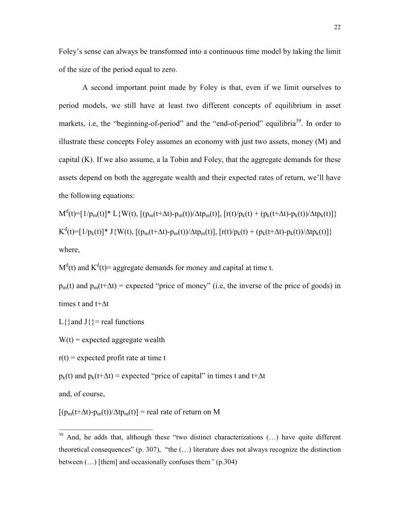
A second important point made by Foley is that, even if we limit ourselves to

period models, we still have at least two different concepts of equilibrium in asset

markets, i.e, the “beginning-of-period” and the “end-of-period” equilibria39. In order to

illustrate these concepts Foley assumes an economy with just two assets, money (M) and

capital (K). If we also assume, a la Tobin and Foley, that the aggregate demands for these

assets depend on both the aggregate wealth and their expected rates of return, we’ll have

the following equations:

Md(t)=[1/pm(t)]* L{W(t), [(pm(t+∆t)-pm(t))/∆tpm(t)], [r(t)/pk(t) + (pk(t+∆t)-pk(t))/∆tpk(t)]}

Kd(t)=[1/pk(t)]* J{W(t), [(pm(t+∆t)-pm(t))/∆tpm(t)], [r(t)/pk(t) + (pk(t+∆t)-pk(t))/∆tpk(t)]}

where,

Md(t) and Kd(t)= aggregate demands for money and capital at time t.

pm(t) and pm(t+∆t) = expected “price of money” (i.e, the inverse of the price of goods) in

times t and t+∆t

L{}and J{}= real functions

W(t) = expected aggregate wealth

r(t) = expected profit rate at time t

pk(t) and pk(t+∆t) = expected “price of capital” in times t and t+∆t

and, of course,

[(pm(t+∆t)-pm(t))/∆tpm(t)] = real rate of return on M

39 And, he adds that, although these “two distinct characterizations (…) have quite different

theoretical consequences” (p. 307), “the (…) literature does not always recognize the distinction

between (…) [them] and occasionally confuses them” (p.304)

23

and

[r(t)/pk(t) + (pk(t+∆t)-pk(t))/∆tpk(t)] = real rate of return on K

In the “end-of-period” equilibrium, according to Foley (p.309), “demands and

supplies [of assets] are offered as of the end of the period. Agents can offer to sell K, for

instance, which does not exist at the trading moment but which they plan to produce

during the period. Contracts are made for labor and capital services and consumption

during the period and asset deliveries at the end”. So, in this case we have that the

relevant supplies of assets are the supplies available at the end of the period (i.e, the

supplies available in the beginning of the period, M(0) and K(0), plus the additions

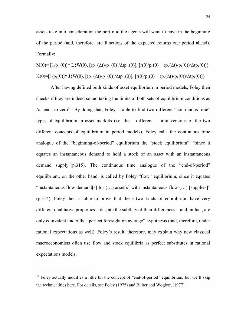
created within the period, ∆M and ∆K) and the relevant demands for assets take into

consideration the portfolio the agents will want to have in the beginning of the next

period (and, therefore, are functions of the expected returns two periods ahead).

Formally:

M(0)+∆M=[1/pm(∆t)]*L{W(∆t),[(pm(2∆t)-pm(∆t))/∆tpm(∆t)],[r(∆t)/pk(∆t)+(pk(2∆t)-

pk(∆t))/∆tpk(∆t)]}

K(0)+∆K=[1/pk(∆t)]*J{W(∆t),[(pm(2∆t)-pm(∆t))/∆tpm(∆t)],[r(∆t)/pk(∆t)+(pk(2∆t)-

pk(∆t))/∆tpk(∆t)]}

In the “beginning-of-period” equilibrium, on the other hand, “trading in and

delivery of assets are assumed to take place at the same time, that is, the beginning of the

period. Within period consumption is contracted for but within-period production is done

on a kind of speculation” (Foley, p.310). So, in this case we have that the relevant

supplies of assets are the supplies available at the beginning of the period (M(0) and

K(0), i.e, the stocks inherited from the previous period) and the relevant demands for

24

assets take into consideration the portfolio the agents will want to have in the beginning

of the period (and, therefore, are functions of the expected returns one period ahead).

Formally:

M(0)= [1/pm(0)]* L{W(0), [(pm(∆t)-pm(0))/∆tpm(0)], [r(0)/pk(0) + (pk(∆t)-pk(0))/∆tpk(0)]}

K(0)=[1/pk(0)]* J{W(0), [(pm(∆t)-pm(0))/∆tpm(0)], [r(0)/pk(0) + (pk(∆t)-pk(0))/∆tpk(0)]}

After having defined both kinds of asset equilibrium in period models, Foley then

checks if they are indeed sound taking the limits of both sets of equilibrium conditions as

∆t tends to zero40. By doing that, Foley is able to find two different “continuous time”

types of equilibrium in asset markets (i.e, the – different – limit versions of the two

different concepts of equilibrium in period models). Foley calls the continuous time

analogue of the “beginning-of-period” equilibrium the “stock equilibrium”, “since it

equates an instantaneous demand to hold a stock of an asset with an instantaneous

demand supply”(p.315). The continuous time analogue of the “end-of-period”

equilibrium, on the other hand, is called by Foley “flow” equilibrium, since it equates

“instantaneous flow demand[s] for (…) asset[s] with instantaneous flow (…) [supplies]”

(p.314). Foley then is able to prove that these two kinds of equilibrium have very

different qualitative properties – despite the subtlety of their differences – and, in fact, are

only equivalent under the “perfect foresight on average” hypothesis (and, therefore, under

rational expectations as well). Foley’s result, therefore, may explain why new classical

macroeconomists often use flow and stock equilibria as perfect substitutes in rational

expectations models.

40 Foley actually modifies a little bit the concept of “end-of-period” equilibrium, but we’ll skip

the technicalities here. For details, see Foley (1975) and Buiter and Woglom (1977).

25

1.3 - The SFCA and Post Keynesian Macroeconomics

The aim of this part of the paper is to discuss – in an introductory and non-

exhaustive way - the case for the wide adoption of the SFCA by Post-Keynesians as

presented by Lavoie and Godley (2001-02, p.131). According to these authors:

“Post Keynesian economics, as reported by Chick (1995), is sometimes accused of lacking coherence,

formalism, and logic. (…). The stock-flow monetary accounting framework provides (...) an alternative

[logical] foundation [for Post-Keynesian macroeconomic modeling] that is based essentially on two

principles. First, the accounting must be right. All stocks and all flows must have counterparts somewhere

in the rest of the economy. The watertight stock flow accounting imposes system constraints that have

qualitative implications. This is not just a matter of logical coherence; it also feeds into the intrinsic

dynamics of the model”.

We’ll discuss this claim in two steps. First, we’ll present the SFC critique of the

Keynes/Kalecki conventional short run macroeconomic equilibrium, still widely used by

Post-Keynesians in general41. Second we’ll discuss in more general terms what may go

wrong when one doesn’t take SFC requirements into consideration. While the arguments

that follow are hardly new, we hope they will convince the reader of the crucial

importance of the issue at hand.

1.3.1 - Stock-flow inconsistency in the GT

As mentioned in the first part above, the SFC critique of the Keynes/Kalecki

notion of short run equilibrium was the reason why the SFCA appeared in the first place.

We chose to discuss it here for three reasons. First because it is an important particular

example of the general point that Lavoie and Godley are trying to make, i.e, that the

41 See, for example, Davidson (1994), Lavoie (1992) and Palley (1996).

26

adoption SFCA offers more insight than (and may correct logical problems of) current

practices. Second because, as mentioned before, versions of the Keynes/Kalecki short run

equilibrium are still widely used today despite their logical problems. Third, because we

strongly believe that Keynes and Kalecki were essentially right in their particular

formulations and we hope this will highlight the constructive nature of the SFC critique42.

One of the reasons why the discussion of Keynes’s short run equilibrium is useful

to highlight the distinguishing features of the SFCA – though certainly not the most

important – is that the exact meaning of this particular concept has been the object of

intense controversy over the years43. SFC authors, on the other hand, use formal models

of the whole economy that enable the reader to “pin down exactly why the results come

out as they do”, as opposed to other “writings on monetary theory” that “rely solely on a

narrative method which puts a strain on the reader’s imagination and makes

disagreements difficult to resolve” (Godley, 1999, p.394). Be that as it may, we’ll avoid

here all the discussion about “what Keynes really meant” and follow chapter XVIII of the

General Theory as closely as possible.

As it is well known, in chapter XVIII Keynes divide the variables in his model in

three groups, i.e. “given”, “independent” and “dependent”. He called the first two groups

the “deteminants of the economic system” (the third comprises his endogenous variables)

and added:

42 Even though the following discussion will focus on Keynes, we hope it will be clear that the

critique is valid for both authors. 43 For two of the many different interpretations of “the exact meaning” of Keynes’s short run

equilibrium, see Amadeo (1989) and Asimakopulos (1991). Many others exist and we don’t want

to imply here that none of them is SFC.

27

“the division of the determinants of the economic system into two variables is, of course, quite arbitrary

from any absolute standpoint. The division must be made entirely on the basis of experience, so as to

correspond on the one hand to the factors in which the changes seem to be so slow or so little relevant to

have only a small and comparatively negligible short term influence in our quaesitum [i.e, the “given”

variables]; and on another hand to those factors in which the changes are found in practice to exercise a

dominant influence in our quaesitum” [i.e, “independent” variables]. (Keynes, GT, ch. XVIII, p.247)

As is also well known, Keynes explicitly listed the stock of capital and labor

among the “given” variables and, therefore, as noted by Hicks and Asimakopulos,

Keynes’s short run “represents an interval of time sufficiently brief so that changes

during this interval in productive capacity, that occur continuously in any economy with

positive net investment, are small relative to the initial productive capacity so that they

can be legitimately ignored. This interval, however, must also be sufficiently long for

most of the multiplier’s effects of a change in investment to have been completed within

that period” (Asimakopulos, 1991, p.68).

But what about other macroeconomic stocks? What did Keynes have to say in the

GT, for example, about macroeconomic stocks like the public debt, private wealth or the

economy’s foreign debt? Not much, really. However, as Tobin (1980, p.75) points out,

“though Keynes was not explicit about assets other than capital, the spirit of the approach

is presumably the same: the time span for which the model is intended is too short for

flows to make noticeable changes in stocks” (Tobin, 1980, p.75).

At this point, we must be ready to understand the SFC critique of Keynes’s notion

of short run equilibrium as described in chapter XVIII of the GT. The problem – to put it

briefly – is that if one thinks about stocks in general (and not only the stock of capital),

especially financial stocks, it doesn’t really make sense to think of them as “given”

28

variables. As noted by Tobin in his Nobel Conference, that’s precisely why "the

interpretation of the solution to a Keynesian short-run macroeconomic system has always

been ambiguous. (…) Is the solution an equilibrium in the sense of a position of rest?

This can hardly be the case for a model whose very solution implies changes in the stocks

of capital, wealth, government debt, and other assets. Since the structural equations of the

model depend on those stocks, they will not replicate the solution when the stocks are

moving. Keynes himself recognized the problem but excused himself for ignoring the

dynamics of accumulation by defining the horizon of the analysis as short enough so that

flows make insignificant difference to the size of stocks. The excuse makes tolerable

sense for the stocks of physical capital and total wealth, but unbalanced government

budgets, monetary operations and external imbalances can alter the corresponding asset

stocks quite rapidly. A model whose solution generates flows but completely ignores

their consequences may be suspected of missing phenomena important even in a

relatively short-run, and therefore giving incomplete or even misleading analyses of the

effects of fiscal and monetary policies". (Tobin, J, 1982, p. 188).

1.3.2 - What exactly are the problems? - A Summary

A lot of things happen when one takes explicitly into account all stock-flow

relations implicit in Keynes’s equilibrium. First, as mentioned before, Keynes’s static

system turns into a dynamic one. Second, one gets a series of new variables to explain.

Clearly, for example, the flow of net investment adds to the size of capital stock. What is

then the influence of this increased stock in the subsequent flows of investment and

income? Any explicit theoretical answer to this question, whatever it might be,

29

necessarily involves an assertion about stock(of capital)-flow(of investment or of income)

ratios. Stock-flow ratios are at the core of most of current policy-relevant issues. How

does the size of government debt affect interest rates (and through this channel) GDP?

What’s the optimum external debt to exports ratio for under-developed countries? How

does the private stock of wealth (including the stock market part of it) affect the flows of

consumption and imports? What does conventional Post Keynesian (or Keynesian, for

that matter) economics have to say about these crucial issues? The first general point to

be made here is precisely that stock-flow ratios play a crucial role in modern capitalist

economies and, therefore, models of these economies must necessarily include them.

Surely one can’t do that without theorizing about them. The need for this continuing

theorizing effort is a second general point being made here.

To state that Post-Keynesians in general don’t know much about stock-flow ratios

doesn’t mean, of course, to state Post-Keynesians don’t now anything at all about them.

There are, of course, many Post-Keynesian models dealing with stock-flow issues44. The

problem here is that it is not clear how much their conclusions are affected by the stock-

flow inconsistency bias. So, the third general point being made here is precisely the one

made by Tobin about Keynes. If a model generates flows it has to deal with all their

consequences, otherwise it may very well give misleading analyses.

The fourth and last point we want to make here – related to the third above - is

that, as we’ll discuss below, when one explicitly takes into consideration all the flow-

flow, stock-flow and stock-stock relations implicit in a given macroeconomic model of

44 Again, a detailed list would be beyond the scope of this paper. Two examples are Thirwall’s

growth model (see, for example, McCombie and Thirwall, 1994, ch.3) and Davidson’s

interpretation of chapter 17 of the G.T (see, for example, Davidson, 1972, ch.4).

30

hypotheses (that is, if one works with a closed system in which every flow comes from

somewhere and goes somewhere), one gets to know all the (often non-trivial) “system-

wide” logical requirements implicit in the system at hand and these impose a lot of

structure in the models.

1.4 - Some notes on the “state-of-the-art” of SFC work

SFC model building has gone a long way in the last two decades, especially since

the second half of the 1990s45. A common SFC methodology – based on the pioneering

work by Brainard and Tobin (1968) and refined by Wynne Godley in a long series of

papers – has been established and its application to a series of socially relevant policy

issues has shed light on many previously “dark” areas. Yet, the SFCA is still relatively

recent and a lot remains to be done. In what follows we’ll attempt to summarize the main

features of the recent SFC literature. Hopefully, this summary will convince the reader

that this line of research is a clear and progressive alternative to current mainstream

macroeconomics.

1.4.1 - The Tobin-Godley methodology for theoretical work in macroeconomics

In somewhat schematic terms, the consensual methodology implicit or explicit in

the recent SFC literature consists of three steps, which are: (i)do the (SFC) accounting

first; (ii)establish the relevant behavioral relationships after that; and then (iii) perform

“comparative dynamics” exercises (generally with the help of computer simulations) to

see how the model behaves. As this description makes clear, as does our interpretation of

45 See footnote 6 for a representative sample of recent SFC work.

31

the SFCA as a natural development of the Keynesian research program, this Tobin-

Godley methodology has close similarities to the one implicit in the “old” Keynesian

models. As this fact may give the reader the wrong impression that there’s nothing really

new being said in the recent SFC literature, it seems appropriate to emphasize here the

differences between these two methodologies46.

Beginning with the first point, we mentioned before several reasons why SFCA

authors rely so much on consistent accounting frameworks. In practice this means that the

first thing a SFC theorist must do in order to analyze a given issue is to make sure he or

she has an “adequate” SFC accounting framework to deal with it47. There are no

exceptions to this rule, no matter the kind of issue being analyzed. If no such accounting

framework exists, the SFC theorist has to design it herself. Data availability is, in fact,

irrelevant in this first step. What the theorist gets from this accounting exercise is the

whole set of “system-wide” logical requirements that are relevant to the issue at hand.

These come in three kinds. First, there is the “intrinsic SFC dynamics of the system”, i.e,

the fact that flows necessarily increase or decrease stocks and these, by their turn,

influence future flows. Second, there are the “sectoral budget constraints”, i.e, the fact

that in each accounting period the decisions of economic agents alone and in the

aggregate are constrained by what they have in the beginning of the period48, what they

earn during the period and their access to credit. Third, there are the “adding up”

46 See, for example, Klein and Young (1980) for a nice example of an “old” neoclassical

Keynesian “flow” macroeconometric model. Modern expositions of the “Cowles Commission

approach” (like Fair, 1984) are very close to the Tobin-Godley methodology, though. 47 We don’t want to imply that the choice of the “adequate” accounting framework is independent

of theoretical considerations, though. The contrary is true, as argued in the first part of this paper. 48 Subject also to liquidity constraints, as Keynes would have emphasized.

32

constraints, i.e, the fact that accounting identities imply that the whole must necessarily

equal the parts and certain (combinations of) stocks and flows must necessarily equal

others. Concentrated attention on these logical requirements differentiates SFC macro

models from conventional Keynesian ones. Many authors explored some implications of

some of these logical requirements in the past, but very few of them realized/emphasized

the importance of always trying to explore all the implications of all of them.

A careful analysis of these requirements has important implications also for the

choice of the behavioral equations of the model, the second step of the Tobin-Godley

approach49. First, the use of SFC accounting frameworks makes clear the necessity to

theorize about stock-flow ratios (since they have non-trivial dynamic implications).

Second, and perhaps more obvious, the use of any accounting framework implies a given

number of degrees of freedom to the system and this limits the number of possible

“model closures” as discussed in the first part of this paper. Note, however, that in

complex accounting structures the nature of these degrees of freedom may not be obvious

at first sight. In particular, the use of a water-tight SFC accounting framework implies

that in an economy with n sectors, the financial flows of the nth sector are completely

determined by the financial flows of the other n-1 sectors of the economy50. This fact has

nothing to do with the neoclassical concepts/assumptions such as Walras’s Law, utility

maximizing individual agents, market equilibrium and etc. It happens simply because

what sectors 1 to n-1 (in the aggregate) pay to sector n is equal to what sector n receives

from these sectors and vice-versa.

49 Along, of course, with other theoretical considerations and more traditional concerns with the

“structure” of the economy at hand (that are also present in the choice of the accounting itself). 50 See Godley, 1996 and 1999.

33

After the first two steps what one generally gets is a complicated system of non-

linear difference/differential equations. The third step, naturally, is to perform a series of

comparative dynamics exercises to evaluate the sensitivity of the model dynamics to

changes in parameters and key exogenous variables. Given that analytic solutions to these

systems are seldom available, SFC practitioners often must use computer simulations to

try to approximate them. As Godley (1996, p 22) puts it, this approximation is often good

in practice:

“(…) with numerical solutions (…), we can gain insights into how the system as a whole functions, by first

obtaining a base solution and then changing one exogenous variable at a time to see what difference is

made. It might seem as a though any particular model “run” depends so much on the particular numbers

used that the results are completely arbitrary and have no general application at all. However, it is my

experience that repeated simulation, combined with iterative modification of the model itself, does

progressively lead to improved understanding, for instance, of what the stability of the system turns on,

what combinations of parameters are plausible and how the whole thing responds when subjected to

shocks”.

The schematic presentation above should not lead the reader to believe the three

steps are taken independently. There is a lot of “back and forth” movement between them

and, as mentioned before, a lot of “art” is involved in the model building process.

However, SFCA authors strongly believe that this methodology provides a logical and

coherent way to approach macroeconomic issues.

1.4.2 - Recent Developments and Unknown Territory

The recent SFC literature has both “destructive” and “constructive” sides. In fact,

many recent papers have used the SFCA to find inconsistencies in existing

macroeconomic models. So Taylor (1998a, 1999 and 2002), for example, has argued that

34

the famous Mundell-Fleming model is logically inconsistent because when “full SFC

accounting is respected” it can be shown that it “has one fewer independent equation than

one usually thinks”, while Godley and Shaikh (2002) have argued that the standard (neo)

“classical” macroeconomic model is also stock-flow inconsistent and, although it can be

fixed with “minor changes”, the consequences of these changes are far from “minor”.

One must not overemphasize this “destructive” side of the SFCA literature, though.

Indeed, not only does the use of the SFCA help to identify inconsistencies in existing

macroeconomic models, but it also (almost simultaneously, in fact) helps to fix them. So

all the papers mentioned above offered SFC alternatives to the previously inconsistent

models they criticized.

Also on the constructive side, the SFCA has recently been used to shed light on a

number of policy relevant issues. So, while Taylor (1998b) has used it to criticize the

plausibility of current mainstream models of speculative attacks and financial crises and

propose a new one, Godley and Lavoie (2002) have used it to study complex monetary

arrangements like, for example, the European Monetary Union and Izurieta (2002) has

used it to analyze the consequences of dollarization schemes. As mentioned before,

“new” SFC work sometimes requires the construction of “new’ SFC accounting

frameworks. Indeed, both Taylor (in his critique of the Mundell-Fleming model) and

Godley and Lavoie(2002) and Izurieta (2002) (in their analyses of the EMU and

dollarization schemes), for example, used versions of Godley’s original accounting of

“two interdependent economies which together form the whole world” in their papers51.

51 See Godley (1999b) for details.

35

The “frontier” of the SFCA is not limited to finding inconsistencies in existing

macroeconomic models and developing new SFC accounting frameworks and models for

new problems, though. Although a discussion of empirical SFC models would have

extended this paper far too long, these models have continuously been used for policy

analysis in the last decades52. Empirical specifications of SFC models involve a large

number of unsettled issues related to the transition from theoretical to empirical

macroeconomic models. There’s no consensus, for example, about “applied” issues such

as the choices of (i) the size of models, (ii) their degree of aggregation, (iii) the relevant

accounting period, (iv) the relevant econometric techniques and etc. Research on SFC

models, therefore, can conceivably benefit from current research in selected fields of the

mainstream, like those related to computer simulated agent-based models (that might

illuminate issues related to aggregation), application of optimal control theory to policy

analysis and advances in macroeconometric techniques, for example.

1.5 - Conclusion

Stock-Flow consistency can be seen from different angles. As we tried to argue,

people that strongly believe in the efficiency and speed of the self-adjusting properties of

markets tend to see it as a mere detail that can be trivially met and probably can be

ignored without it causing any major problems. People that don’t believe that markets

and agents are (or even can be) so rational and informed, on the other hand, tend to

52 See, for example, Davis (1987a and 1987b), the SFC papers in Taylor (1990) and Alarcon et.al.

(1991) and the series of “applied” papers by Wynne Godley both at the Department of Applied

Economics of the University of Cambridge and at the Levy Economics Institute (like, for

example, Godley, 1999c).

36

believe (or, at least, should admit the possibility) that SFC requirements impose a great

deal of structure in an otherwise extremely unpredictable economic environment.

Therefore, although both sets of economists are advised to pay careful attention to these

requirements and issues, this paper tried to argue that the second set has much more

reasons to do so than the first.

This paper also attempted to present a summary of the current “state-of-the art” of

the SFCA research. Although it’s impossible to make justice to both the breadth and the

potential implications of current research in a couple of pages, we hope to have given

enough evidence of the continuous progress made by SFC authors in the last two decades

and of the possibilities of this line of research.

37

2 - Cambridge and Yale on Stock-Flow Consistent Macroeconomic Modeling

Introduction

The last 5 years have witnessed a revival of the stock-flow consistent approach to

macroeconomic modeling (SFCA) that was at the frontier of Keynesian research in the

seventies and eighties53. SFC models didn’t receive proper attention at that time –

dominated by the endless debates that followed the so-called New Classical “counter-

revolution” – and, with notable exceptions, practically disappeared from the literature for

a while. However, with most of the profession now convinced that New Classical

economics doesn’t offer convincing explanations for the dynamics of actual economies in

historical time, macroeconomists of all sorts are increasingly rediscovering old truths.

This process is not an easy one, though. It’s just symptomatic that the modern “New

Keynesian consensus” has been criticized precisely for neglecting the stock-flow

relations emphasized by the SFCA54.

Part of the problem is that, given their emphasis on “water tight” accounting

frameworks, SFC authors and models are often perceived as either national accountants

(accounting) or “applied economists” (economics). This is a truth, but only a half-truth55.

Proper stock-flow consistent accounting imposes a great deal of structure to

macroeconomic models by making their “system-wide” logical implications clear to the

analyst. It also makes explicit the need for theorizing about a whole lot of “forgotten”

53 As discussed in section 1.4.2 above. 54 As seen in section 1.2.2 above. 55 It’s true, in particular, that SFC macro models are often used (as any good macro theory

should) in applied research and are based on national accounting schemes. E.P Davis (1987a and

1987b), L.Taylor (1990), Alarcón et.al. (1991) and Godley (1999b) provide many examples of

applied SFC macro models.

38

variables (i.e., the ones that do not appear in stock-flow inconsistent models, though

logically implied by their hypotheses), especially stock-flow ratios56. These are all

theoretical issues, not “applied” ones. Of course, we don’t want to imply here that there

hasn’t been any economic theorizing about stock-flow ratios in the past. What we do

want to imply is that most people that did this theorizing either assumed problems away

with strong hypotheses about rationality of agents and instantaneous market-clearing57 or

didn’t care to phrase their arguments in a proper SFC model58. Although the later group is

clearly more interesting than the first, their message is at best incomplete. As put by

Tobin (1982, p.188), “a model whose solution generates flows but completely ignores

their consequences may be suspected of missing phenomena important even in a

relatively short-run, and therefore of giving incomplete or even misleading analyses

(…)”.

Indeed, even though the number of possible “closures” for any reasonably

realistic SFC accounting framework is huge59, very few authors have written reasonably

complete SFC models in the proper sense of the term and one can clearly distinguish in

these writings a “Yale” (or Brainard-Tobin-type) and a (New) “Cambridge” (or Godley-

56 Which, by the way, are at the core of many unresolved policy issues. Just to mention two

among many other possible examples, what policy-makers think about the public debt to gdp

ratio and the external debt to exports ratio will probably determine to a good extent the supply of

public and imported goods that will be made available to the people. It’s symptomatic that most

Keynesian macro has focused only on static variables like the public debt or the rate of inflation

and (to a reasonable extent) neglected dynamic ones. 57 See Foley (1975) for a proof that stock and flow equilibria are indistinct under rational

expectations. 58 This is the case of heavy-weights like Friedman, Harrod, Hicks, Meltzer and Modigliani,

among many others.

39

type) types of “closures”60. As mentioned before, most of these ideas were written in the

seventies and eighties and, yet, we hope to demonstrate in what follows that they deal in a

careful and profound way with many theoretical issues that are still open as of today. In

fact, a second goal of this paper is precisely to provide a context for the current SFC

discussion.

Note, however, that SFC authors have written extensively about issues so

different as the behavior of banks, financial markets in general, industrial pricing, wage

determination and open-economy macroeconomics. Although all these issues can be seen

as part of the broad SFCA research program, we will restrict ourselves here to the

discussion of what these authors had to say about macroeconomic models of closed

economies with Fixprice goods’ market and Flexprice financial markets61. This decision

means that one must regard this paper as an introductory effort. In particular, most SFC

discussion in the seventies and eighties (especially at Cambridge) dealt with inflation

accounting and open-economy issues and these are neglected here.

In what follows we do four things. First, we present the (SFC) accounting

framework of the closed “artificial economy” that will be used in this paper and a couple

59 As stressed by Taylor (1990, p.46) 60 Examples of Yale-type models are Brainard and Tobin (1968), Foley (1975), Tobin and Buiter

(1976), Braga de Macedo and Tobin (1979), Backus et.al. (1980) and Tobin (1982). The British

team is represented by Cripps and Godley (1976), Godley and Cripps (1983), Anyadike-Danes

et.al. (1987) and Godley and Zezza (1989), among others. We don’t want to imply, of course,

that other authors didn’t write related material at that time. Fair (1974, 1984 and 1994) is an

obvious example from Yale, but note that, as he put it himself, “what is commonly referred as

“Yale macro” is quite different in emphasis from (…) [his] own work” (Fair, 1984,

acknowledgments).

40

of generic theoretical issues related to the SFCA. After that, we discuss formally the

characteristics of both our (somewhat stylized) Yale-type (in section 2.2) and (New)

Cambridge-type (in section 2.3) “closures” of the accounting framework presented

before. The fourth section discusses briefly some recent work by Godley (1996, 1999)

and Lavoie and Godley (2001-2002) that propose a synthesis of the two “pure” models

presented in the previous parts.

2.1 - The Accounting framework and its implications

This part of the paper is divided in two sections. Section 2.1.1 below presents the

“artificial economy” we will use as a “neutral theoretical court” in which the arguments

of both schools can be presented and compared62. Section 2.1.2 discusses a couple of

theoretical issues that usually arise in such discussions.

2.1.1 - The artificial economy

In our artificial economy there are (a) four “macroeconomic sectors”, i.e.,

households, government, (non-financial) firms and banks, (b) six assets, i.e., high-

powered money (currency and bank reserves), demand deposits, time deposits,

government bonds, business equity and business loans and (c) one produced good63.

Table 1 below summarizes the main characteristics of the economy at hand.

61 In other words, we’ll be reducing important theoretical issues either to specific behavioral

hypotheses or to specific parameters of a macro model of a closed economy. 62 We leave to the reader the task of judging the neutrality of our framework, though. 63 This “one good economy” hypothesis is characteristic of Yale-type models (see Backus et.al.,

1980, p.263). Cambridge economists, on the other hand, have always tried to theorize directly

about aggregates. For convenience, we chose here to phrase Cambridge models in terms of Yale

41

Beginning with the households, our simplifying assumptions – made only for

convenience - are that (i) they don’t have access to credit, (ii) they don’t invest, (iii) their

wealth is divided among five possible assets (i.e., cash, money and time deposits, equity

and government bonds), (iv) they don’t pay taxes, and (v) their total income consists of

wages, dividends and interest payments on bonds and time deposits. A close look at

Table 1 below is probably more informative than any written description, though. The

upper part of the table accounts for the current transactions made in the economy64, so

hypotheses (ii), (iv) and (v) should be obvious just by inspection of the upper part of the

households’ column (note that a plus sign before a variable indicates that money is being

earned, while a minus indicates that money is being spent). The lower part of the table

accounts for the consequences of the transactions in the first part over the total wealth of

the sectors (summarized by the “current savings” of the sectors) and the “capital

transactions”, i.e., the changes in the composition of these stocks of wealth (a plus sign in

this case indicates a source of funds, while a negative sign indicates a use of funds).

Again, it takes only a look at the lower part of the households’ column to get assumptions

(i) and (iii) right.

ones. The alternative – unavoidable in empirical work – would have forced us to deal with

complicated price and volume indexes. 64 With the exception of purchases of “capital” and inventory accumulation by firms. These are

both current receipts (from the point of view of firms that sold them) and capital expenditures

(from the point of view of firms that acquired them).

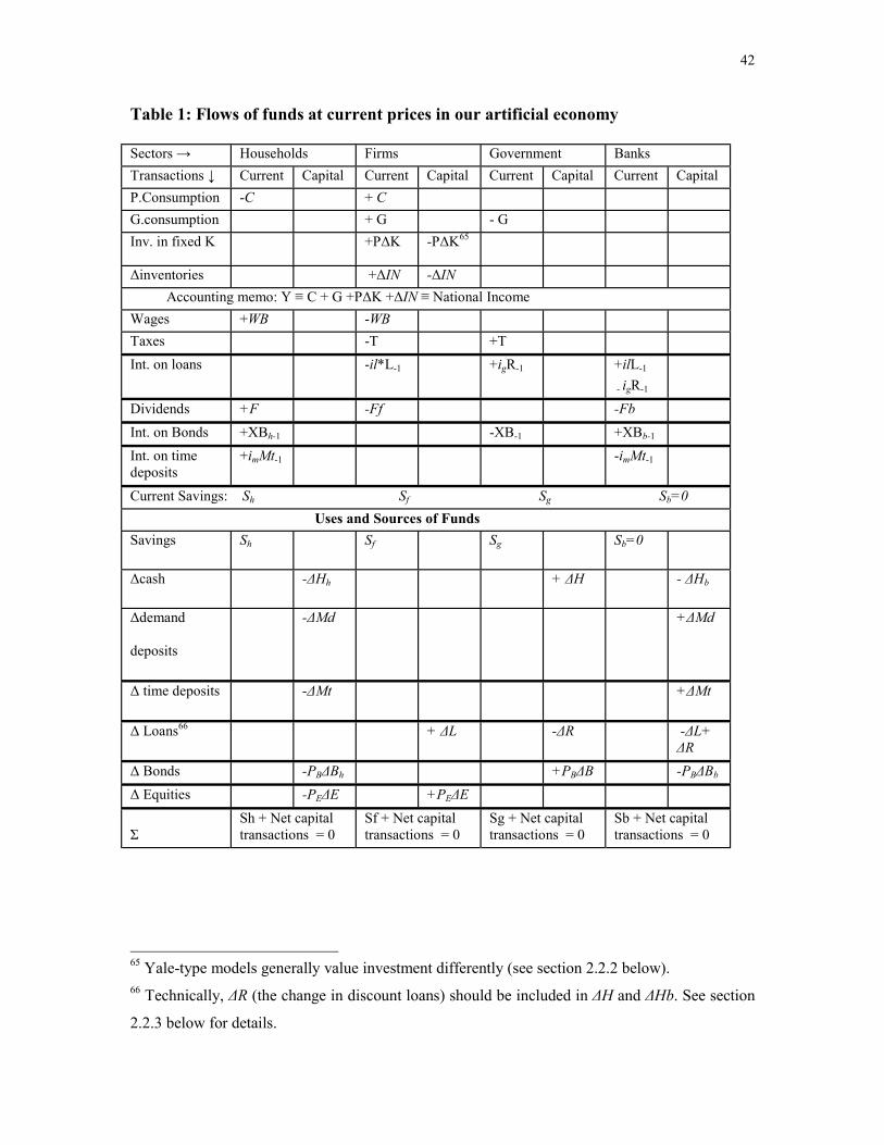
42

Table 1: Flows of funds at current prices in our artificial economy

Sectors → Households Firms Government Banks Transactions ↓ Current Capital Current Capital Current Capital Current Capital P.Consumption -C + C G.consumption + G - G Inv. in fixed K +PΔK -PΔK65

Δinventories +ΔIN -ΔIN Accounting memo: Y ≡ C + G +PΔK +ΔIN ≡ National Income Wages +WB -WB Taxes -T +T Int. on loans -il*L-1 +igR-1 +ilL-1

- igR-1

Dividends +F -Ff -Fb Int. on Bonds +XBh-1 -XB-1 +XBb-1 Int. on time deposits

+imMt-1 -imMt-1

Current Savings: Sh Sf Sg Sb=0 Uses and Sources of Funds Savings Sh Sf Sg Sb=0

Δcash -ΔHh + ΔH - ΔHb

Δdemand

deposits

-ΔMd +ΔMd

Δ time deposits -ΔMt +ΔMt

Δ Loans66 + ΔL -ΔR -ΔL+ ΔR

Δ Bonds -PBΔBh +PBΔB -PBΔBb Δ Equities -PEΔE +PEΔE Σ

Sh + Net capital transactions = 0

Sf + Net capital transactions = 0

Sg + Net capital transactions = 0

Sb + Net capital transactions = 0

65 Yale-type models generally value investment differently (see section 2.2.2 below). 66 Technically, ΔR (the change in discount loans) should be included in ΔH and ΔHb. See section

2.2.3 below for details.

43

Turning now our attention to businesses, we assume for simplicity that all the

goods and services of the economy are produced by firms (so banking services, for

example, are not assumed to be part of GDP). As should be clear from the inspection of

the upper part of the firms’ column of Table 1 above, retained profits of firms are

assumed to be equal to their total (final) sales (C+ G+PΔK) plus their net acquisition of

inventories minus their payments of wages, taxes, interest on loans and dividends to

owners. The inspection of the firms’ uses and sources of funds, on the other hand, makes

clear that we are assuming that they finance their accumulation of capital with loans,

equity emissions and retained earnings (Sf). We are, therefore, assuming away (i) private

bonds as a possible source of funds for firms and (ii) financial speculation by firms (since

they don’t keep wealth in the form of financial assets).

The government (assumed here to include a central bank), by its turn, gets its

income from taxes (assumed, for simplicity, to be paid only by firms) and interest

payments received on discount loans to banks. Its expenses are purchases of goods and

services from firms and interest (on debt) payments to banks and households67. Again for

simplicity, government debt is assumed to consist only of perpetuities, i.e. bonds that pay

a fixed amount of money ($X) per period. The assumption is that these bonds are traded

in a market and, therefore, have a price PB. As a consequence, the value of the stock of

public bonds at any given period will be PBB, i.e. the price of each bond (PB) times the

number of bonds owned by the public (B). Public deficits (surpluses) are supposed to be

financed (used) either by (with) increases (decreases) in high-powered money or by

(with) sales (purchases) of public bonds.

44

Finally, banks receive interest payments from firms (on their loans) and

government (on their government bonds). Their expenses consist of interest payments on

time deposits and rediscount loans. To avoid unnecessary accounting complications, we

are assuming that (i) banks don’t need workers or fixed capital to operate and (ii) all their

profits are distributed to their owners. Their assets consist of reserves, public bonds and

loans to firms (but, for simplicity, no equities) and their liabilities consist of their deposits

and (if necessary) discount loans from the Central bank.

2.1.2 - Some specific theoretical issues related to the SFCA

A matrix like the one in Table 1 above implies a huge number of theoretical

issues that ultimately have to do with the very definition of macroeconomics. We are well

aware, in particular, that analyses about aggregates necessarily imply a large number of

more or less arbitrary assumptions, all of which can very well be questioned. However, as

our present purpose is not to discuss the macroeconomic method in general, we will

restrict ourselves to a couple of theoretical issues closely related to the SFCA.

First, we’d like to discuss more closely the “system-wide” implications mentioned

above. The first thing to note is that ex-post all rows in Table 1 above add up to zero68.

This is a straightforward consequence of the fact that what one sector pays to the others is

exactly equal to what the others receive from it, but has the non-trivial implication that

the accounts of the n-th sector of the economy are completely determined by the accounts

67 So other assumptions – made only for convenience and explicit in the Table 1 above - are that

the government doesn’t invest and all public workers are volunteers. 68 This is not true ex-ante, though. See Moudud (1998, ch.5) and the discussion below for details.

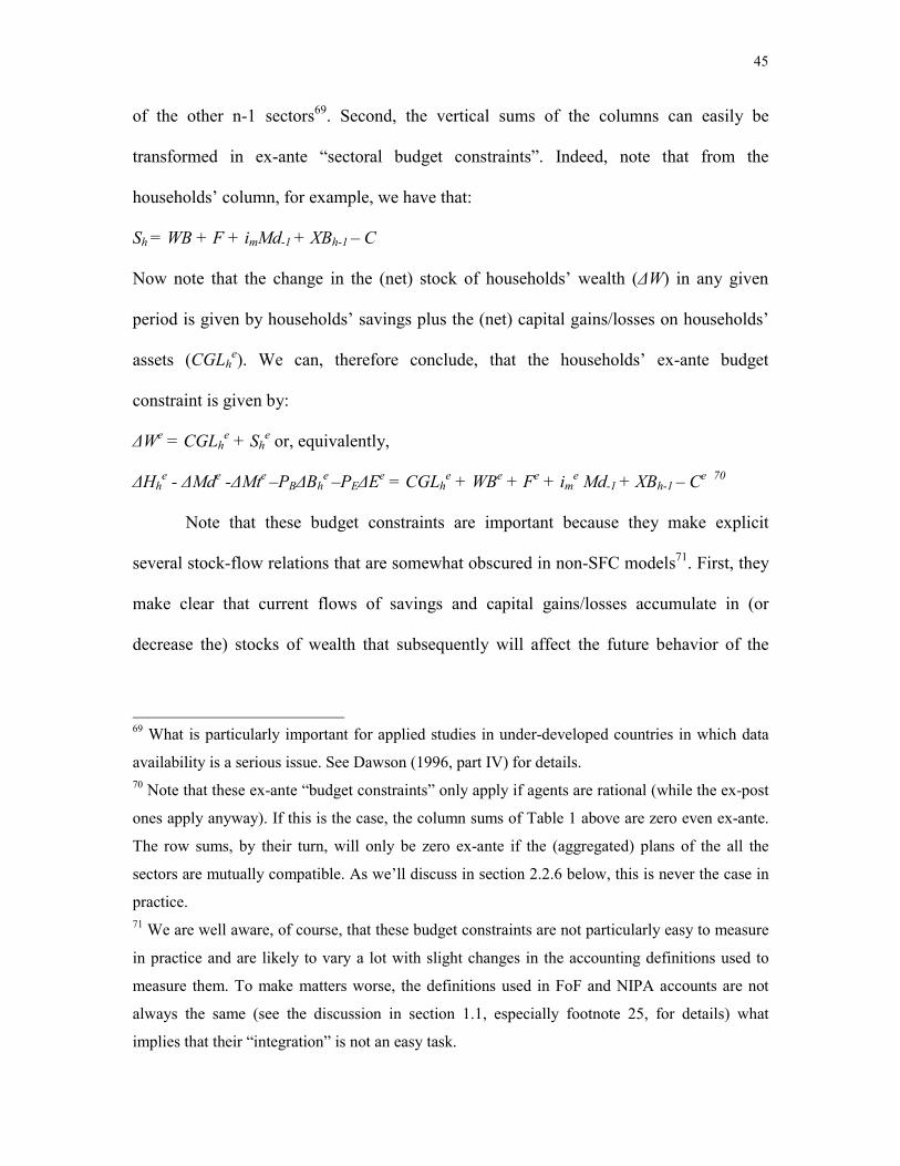
45

of the other n-1 sectors69. Second, the vertical sums of the columns can easily be

transformed in ex-ante “sectoral budget constraints”. Indeed, note that from the

households’ column, for example, we have that:

Sh = WB + F + imMd-1 + XBh-1 – C

Now note that the change in the (net) stock of households’ wealth (ΔW) in any given

period is given by households’ savings plus the (net) capital gains/losses on households’

assets (CGLhe). We can, therefore conclude, that the households’ ex-ante budget

constraint is given by:

ΔWe = CGLhe + Sh

e or, equivalently,

ΔHhe - ΔMde -ΔMte –PBΔBh

e –PEΔEe = CGLh

e + WBe + Fe + ime Md-1 + XBh-1 – Ce 70

Note that these budget constraints are important because they make explicit

several stock-flow relations that are somewhat obscured in non-SFC models71. First, they

make clear that current flows of savings and capital gains/losses accumulate in (or

decrease the) stocks of wealth that subsequently will affect the future behavior of the

69 What is particularly important for applied studies in under-developed countries in which data

availability is a serious issue. See Dawson (1996, part IV) for details. 70 Note that these ex-ante “budget constraints” only apply if agents are rational (while the ex-post

ones apply anyway). If this is the case, the column sums of Table 1 above are zero even ex-ante.

The row sums, by their turn, will only be zero ex-ante if the (aggregated) plans of the all the

sectors are mutually compatible. As we’ll discuss in section 2.2.6 below, this is never the case in

practice. 71 We are well aware, of course, that these budget constraints are not particularly easy to measure

in practice and are likely to vary a lot with slight changes in the accounting definitions used to

measure them. To make matters worse, the definitions used in FoF and NIPA accounts are not

always the same (see the discussion in section 1.1, especially footnote 25, for details) what

implies that their “integration” is not an easy task.

46

economy72. Second, they remind us that the extent to which flows (stocks) are affected by

stocks (flows) depends crucially on their relative sizes. Third, and related to the second,

they make clear that several stock-flow processes are “unsustainable”73, like for example

the ones that imply a sustained growth of debt to income ratios of some sectors (and,

necessarily, sustained growth of wealth to income ratio of the others). In other words,

they remind us of things that cannot happen (say, the sum of the parts be smaller than the

total) but also of things that are not likely to happen (say, a rapid growth of the debt to

income ratio of households or firms continue for a long time74).

A second important theoretical issue to mention is that the accounts above don’t

imply anything about equilibrium concepts or the extent of the (finite) accounting period

used. In other words, they are valid whether the economy is in or out a state of

equilibrium (whatever this might be) and whether the (finite) accounting period under

consideration is an hour or a year75. As Foley (1975) has shown, in period models (i.e.,

models in which the accounting period is finite) there are at least two qualitatively

different (neoclassical) concepts of assets’ equilibrium. As we’ll see in what follows,

Foley’s point is more relevant to the Yale closure than to the Cambridge one (since

Cambridge-type models don’t depend on neoclassical concepts of equilibrium). Be that as

72 Turnovsky (1977, p.xi) calls this stock-flow dynamics the “intrinsic dynamics of the

macroeconomic system”. 73 In the sense of Godley (1999c) 74 Because ceteris paribus this would imply a rapid and continuous increase of the share of

income spent with interest payments and, therefore, a rapid and continuous decrease of the share

of income spent with everything else. The same would be true to the external debt/exports ratio

of a small economy. 75 Changes would have to be made (particularly in the way interest payments are modeled) if the

analysis was in continuous time, though.

47

it may, in what follows whenever a reference is made about events happening in

historical time the assumption will be that the accounting period is a quarter.

2.2 - A Yale-type closure

As phrased by Backus et.al. (1980, p.272-273), the main hypothesis of the Yale

story is that “subject to the budget constraint imposed by (…) prior claims (i.e., “items

that are pre-determined by earlier decisions or by inherited stocks”) a sector is imagined

to formulate long-run target asset and wealth positions, based on current and expected

interest rates, incomes and other relevant variables. Actual positions are then adjusted

toward these targets. Transitory factors like windfall gains and losses will also influence

these adjustments”. Formally this means that, in any given accounting period, all

(aggregate) decision variables of all sectors of the economy should in principle be

modeled as functions of (i) all the variables that determine the sector’s budget constraint

in that particular period and (ii) all the variables that determine the sector’s “long run

target asset and wealth positions” (basically expected future income and real rates of

return of the various assets)76. Indeed, this “general equilibrium approach” is not only a

trademark of Yale-type authors but, in fact, the very starting point of their research

program. As early as 1968, for example, Brainard and Tobin (1968, p.99) wrote that “all

of us seek and use simplifications to oversee the frustrating sterility of the cliché that

everything depends on everything else. But we all know that we do so at some peril. (…)

we argue for the importance of explicit recognition of the essential interdependencies of

markets in theoretical and empirical specification of financial markets”.

48

As one would expect from a research program that extended for several years,

there are many (often subtle) variations of the basic Yale-type story. In what follows

we’ll discuss these subtleties in some detail and try to come up with a “representative”

Yale-type model. For clarity, we’ll denote variables valued at constant prices and all

kinds of rates and ratios by lower case letters and variables measured at current prices

and all kinds of physical stocks by upper case letters.

2.2.1 - Households’ behavioral equations in Yale-type models:

From Table 1 above, it’s clear that the variables in control of the households of

our artificial economy are (i) C (and, given the households’ disposable income, therefore

Sh77) and (ii) the allocation of their stock of wealth W=Hh+Md+Mt+PEE+PBB. As noted

by Fair (1984, p.42), one could also assume that households try to affect their wage bill

(WB) choosing the hours they want to work. Here, however, we’ll work with the

“Keynesian” version of Yale-type models and assume that both the nominal wage and the

general price level (P) are fixed and that the labor supply is perfectly elastic at the given

real wage. In other words, we’ll assume that (in the beginning of each accounting period)

households treat their expected disposable income (to be earned within the period) as a

pre-determined variable.

As put by Tobin (1982, p.187), “the innovation of the [Yale] approach (…) is the

integration of saving and portfolio decisions”. This integration is modeled by assuming

that “households are aiming for end-of-period stocks of value (…) in terms of

76 In disequilibrium specifications one needs also the variables that influence the “adjustment”

process of the portfolios to their long run targets. 77 Keep in mind, however, that our table doesn’t include capital gains or losses.

49

consumption goods at prices of the period. These are functions (…) of current-period

variables – interest rates and expected asset yields, incomes, taxes and etc – and of state

variables determined before the period. The latter include households’ beginning of

period asset stocks” (Tobin, 1980, p.87). In other words, the assumption in Yale-type

models is that the decision variables of the households are all their “real” demands for

assets and these are assumed to be functions of all the variables that determine the

sector’s (expected, real) budget constraint and its “long run target asset and wealth

positions”78. Here we’ll follow Backus et.al. (1980, p.263) and model these demands as

follows79:

78 As mentioned above, it’s crucial in Yale-type models that all demands for assets are modeled as

functions of the same variables. This point, first made by Brainard and Tobin (1968), is

summarized by Tobin (1982, p.173) as follows: “(…) if demand functions are not explicitly

specified for the whole range of assets, the function for the omitted category implied by the

wealth demand function and the explicit asset functions may be strange in ways unintended by

the model-builders. For example, if money demand is related negatively to an interest rate and

total wealth demand is not, the implication is that nonmoney asset functions carry the mirror

image of the interest effect on money. The best practice is to write down all the functions

explicitly, even though one is redundant, and to put the same arguments in all the functions.” 79Yale authors have progressively included more and more variables in the households’ demands

for assets. In the 1968 version of the model, for example, only (within-period) wealth, income

and interest rates are used. Real/nominal distinctions and capital gains and losses weren’t

discussed and savings and portfolio decisions weren’t integrated back then. Tobin (1982, p.184),

on the other hand, presents a “maximalist” specification that includes “four kinds of variables:

those that are within period endogenous (…) lagged variables of the within period endogenous,

expected future variables of within period endogenous; exogenous variables, past

contemporaneous or future”. The “within period endogenous variables” of the (closed economy)

Keynesian version of the model are income and the relevant real rates of return. Tobin was less

specific about the exogenous variables, though, pointing out (1982, p.186) that detailed

specifications of the models would include also considerations about the income distribution and

50

[ad] = f (rhe , rm

e, rbe, re

e, a-1, yde)

where,

a = [Hh/P, Md/P, Mt/Pt, (PB/P)Bh , (PE/P)E] = (hh, md, mt, pBBh , pEE) represents the

households’ real stocks of the various assets; the superscripts “d” and “e” mean “desired”

(or “demanded”) and “expected”; rhe , rm

e, rbe and re

e are the (expected, one period) real

returns in money (either in cash or money deposits), time deposits, government bonds

and equities (respectively, including capital gains); yde is the expected households’ real

disposable income [(WB+F+ imMd-1+XBh-1) /P]e and f: R9→R5 expresses the households’

demands for assets as functions of the various expected real rates of return and the

households’ expected income and previous portfolio. Therefore, the desired change in

households’ real net wealth is given by :

Δwhd= Δhh

d+ Δmdd+ Δmtd+ Δ(pBBh) d+Δ(pEE)d)

i.e., the sum of the components of:

ad - a-1= [Δhhd, Δmdd, Δmtd, Δ(pBBh) d, Δ(pEE) d]

It’s important to notice a couple of things in the formalization above. First, as put

by Coutts and Godley (1984, p.14), it contains “virtually no mention of aggregate (…)

consumption (…)”. The explanation, of course, is that consumption is implied by

households’ savings and expected disposable income. Note, however, that Δwhd is not in

general equal to households’ desired real savings (shd) because, as put by Tobin (1980,

p.88), households are assumed to “(…) take full account of appreciations of existing

age structure of the economy, as well as ““human capital”, expected future wages, taxes and

transfers (…)”.

51

holdings associated with each vector of asset prices” when making their plans80. What

this means in practice is that Δwhd = sh

d + cglhe (expected real capital gains or losses in

households’assets) and, as a consequence, yde and ad (and, therefore, Δwhd) are not

enough to determine desired real aggregate consumption (cd). One needs shd (=Δwh

d -

cglhe), as well. Given yde, ad, and cglh

e, however, one trivially finds shd and cd(= yde- sh

d)

81.

Second, to get to know precisely all the real rates of return and capital gains

involved in the formalization above, we’ll need to add a little more notation. So, let’s call

PA the vector of the prices of assets, so PA = (PH, PMt, PMd, PB, PE) = (1,1,1, PB, PE),

meaning that it costs $PB to buy a government bond, $PE to buy a stock and $1 to get $1

either in one’s wallet or in a bank (either in a money or in a time deposit). Analogously,

let’s call A=(Hh, Md, Mt, Bh, E) the vector of “quantities” of assets. It’s clear, then, that in

the beginning of the period the total nominal stock of wealth of households will be:

W-1=Hh-1+Md-1+Mt-1+ PB-1Bh-1+ PE-1 E-1 = PA-1A-1’

and its “real” counterpart will be:

w-1 = W-1/P-1 = (Hh/P+Md/P+Mt/P+ PBBh/P + PEE/P)-1 = (hh+ md+ mt+ pBBh , pEE)-1

or, equivalently, w-1 =(PA-1A-1’)/P-1

80 Tobin (1980, p.88) recognizes that this hypothesis “(…) may be unrealistic. Household

portfolios may adjust to capital gains and losses only partially within the period they occur,

remaining adjustments occurring later” but adds that it is used only to simplify matters (since, “it

would be possible to modify the specification in this direction”). See section 2.2.6 below for more

on this issue. 81 Note that given, our hypotheses about both banks and non-financial businesses (see below),

households’ disposable income will be equal to the private sector’s disposable income and

therefore YDh – Sh = Ch = C.

52

Now note that, even if the households don’t save/dissave anything (so, A=A-1)

their wealth in the end of the period (both in real and nominal terms) is likely to be

different. Indeed, always keeping in mind that we are assuming inflation away, in this

case we would have82:

W(with Sh=0)= Hh+Md+Mt+ PBBh-1+ PE E-1= PAA-1’ = PAA’

and, therefore, ΔW (with Sh=0)= W-W-1 =(PB- PB-1)*Bh-1 + (PE -PE-1)*E-1= CGLh = P*cglh

Note, finally, that in the general case, Sh won’t be zero. Indeed, (nominal) households’

savings are given by:

Sh=ΔW –CGL h=(Hh+Md+Mt+PBBh+PEE)-(Hh-1+Md-1+Mt-1+PB-1Bh-1+PE-1E-1) -CGLh

or equivalently,

Sh=ΔW –CGL h= PAA’ - PA-1A-1’ - (PB- PB-1)*Bh-1 + (PE -PE-1)*E-1

and, naturally, sh = Sh/P = Δwh - cglh.

The cookbook recipe to calculate the (one period) expected real rates of return of

the relevant assets is the following: first add the expected real value of each asset in t+1

to the expected real value of the receipts associated with the asset in t+1; then divide this

sum by the real value of the asset “today” and subtract one from the result. The one

period expected real rate of return on bonds (rbe), for example, is given by:

rbe =[(PB+1

e/P+1e + X/P+1

e) / (PB/P)] –1 (note that $X= nominal payment for bond in t+1)

or, assuming that P+1e = P, rb

e =[(PB+1e+ X) /PB] –1

Analogously, rme=[(1/P+1

e+ im/P+1e) /(1/P)] –1 (note that im=interest received per dollar in

t+1), or, assuming that P+1e = P, rm

e = im ;

rhe =[(1/P+1

e) / (1/P)] –1 or, assuming that P+1e = P, rh

e = 0 ;

82 As Coutts and Godley (1984, p.14-17) remind us, the accounting gets a little bit more

53

and

ree=[(PE+1

e/P+1+Ff+1e/EP+1)/(PE/P)] –1 (note that Ff+1

e/E=expected dividends per equity in

t+1), or, assuming that P+1e = P, re

e = [(PE+1e+ Ff e/E) /PE] –1

A third thing to note on the formalization above has to do with the concept of

equilibrium implicit in Yale-type models. We took special care with superscripts (that, by

the way, don’t appear in actual Yale-type models) to emphasize a series of unresolved

issues that appear when one thinks about what exactly this equilibrium would mean in

real historical time83. Note, for example, that all “current” variables in the equations

above are only known for sure in the end of the “current” period (so, in the beginning of

the period they are expected as well). A complete macroeconomic equilibrium, then, can

only be reached by either an incredible coincidence or a very competent auctioneer. We’ll

return to this issue in sections 2.2.5 and 2.2.6 below. Note, however, that Yale authors

have emphasized in several passages that their use of the concept of equilibrium is merely

instrumental84.

Note, finally, that the framework above has the advantage of being flexible

enough to accommodate several changes in the hypotheses of the models. In particular, it

can be easily modified to deal with changes in the degree of aggregation of the model and

more financial assets. For example, Yale authors often mention the importance of

distinguishing between wealth-constrained (rich) and liquidity constrained (“young, poor

or both”) households and, therefore, one could conceivably present the model (and a

complicated when inflation enters the picture. 83 For a discussion on the exact meaning of equilibrium positions in period (macro) models, see

section 1.2.3 above, Foley (1975), Buiter and Woglom (1977) and Buiter (1980).

54

corresponding artificial economy) with a more disaggregated households’sector. Note

also that, although Brainard and Tobin don’t model expected income explicitly as a target

variable of households85, their model could conceivably be extended to allow for

“distributive conflict” stories.

2.2.2 - Firms’ behavioral equations in Yale-type models

As put by Backus et.al. (1980, p.265-266), in Yale-type models “business

holdings of financial assets are ignored (…) The [business] sector has two decisions,

investment and financial structure. The later could be further analyzed into two

subchoices: how to finance its new investment, as between loans and equity, and whether

and how to refinance its initial capital”. So it seems fair to say that Yale-type models

don’t deal with the production decisions of firms explicitly (neglecting them in the same

way they do with the income targets of families). This doesn’t mean, of course, that they

are not there. Yale-type models are, in fact, presented in “Keynesian”, “Monetarist” and

“mixed” versions meaning, respectively, models with (i)fixed prices in the goods’

markets, (ii)fixed quantities in the goods’ markets and (iii)a Phillips curve relation

between quantities and prices in the goods’ market. As mentioned before, here we’ll

work with the “Keynesian” fix-price version of the model and, therefore, we’ll interpret

the silence of Yale-type authors about production decisions and inventories as implicit

assumptions that (i) firms are price takers in the market for labor, (ii) their technology is

84 So much that Tobin (1980, p.92) makes reference to the need of a Walrasian auctioneer to solve

it in practice.

55

given, (iii) production is financed by loans repaid in the same period86 and (iv) they are

able to “predict” (or quickly adjust to) the necessary production levels, so ΔIN (the

change in inventories of firms) = 087.

Yale-type models are not particularly clear also about the “financial decisions” of

firms. As stressed by Taylor (1997, ch.1 and 7) and admitted by Tobin (1980, p.90) the

implicit formal hypothesis in Yale-type models is that the Modigliani-Miller theorem

applies and, therefore, the value of the firms’ liabilities (i.e., equities and loans, in Backus

et.al., 1980 or just equities in simpler versions of the model like the ones in Tobin, 1980

and Tobin, 1982) exhaust all the value of its assets (or, in other words, the net worth of

firms is zero). Indeed, if this is the case, “businesses can be modeled as if they are pure

equity firms” (Tobin,1980, p.90), what justifies the explicit hypothesis made in Yale-type

models that “increases in equity occur either by issue of shares or by retention of

earnings; retained earnings are considered as dividends paid matched by sales of shares”

85 As mentioned in the main text households are assumed to target a certain stock (and a certain

composition) of wealth, given their expected disposable income and their total stock of previous

wealth. Fair (1984, p.42) makes a similar point. 86 This seems the only possible way to rationalize it, given that the all profits are distributed and

financial assets of firms are assumed to be always zero. 87 Although Yale authors generally assume that aggregate investment as a whole (including the

change in inventories) is a function of q (see, for example, Tobin, 1982, p.179), it seems possible

to interpret this assumption as a simplifying one. Indeed, we can’t find any reason why changes in

inventories might be considered functions of q and, besides that, almost all American Keynesian

literature has neglected inventory behavior assuming, like Keynes (quoted in Asimakopulos,

1991, p.39), that “the theory of effective demand is substantially the same if we assume that short

period expectations are always fulfilled”. It seems reasonable, then, to rationalize the lack of

importance given to inventory behavior in Yale-type models this way. As we shall see below, this

56

(Backus et.al., 1980, p.266). As stressed by Crotty (1990), this can be interpreted as an

assumption of no conflict between ownership and management, either because they are

both the same or because the first dominates the second.

Things are apparently clearer as far as the “investment decisions” of firms are

concerned. Indeed, one of the trademarks of Brainard and Tobin is their q-theory of

investment and q explains by itself all investment behavior in Yale-type models. As is

well known, q is the ratio between the market valuation of firms’ capital and its

replacement (not historical) cost and first appeared in the literature in Brainard and Tobin

(1968). According to these authors (p.104) the q-theory can be summarized as saying that

“investment is stimulated when capital is valued more highly in markets than it costs to

produce it [i.e., q>1] and discouraged to when its valuation is less than its replacement

cost [i.e., q<1]. Another way to state the same point is to say that investment is

encouraged when the market yield on equity (…) is low relative to the real returns to

physical investment”.

Note, however, that Brainard and Tobin’s (1990) response to Crotty (as well as a

passage in Tobin, 1980, p.90) makes clear that (i)Yale authors are not convinced that the

Modigliani-Miller theorem works so nicely in practice88 and (ii) they are convinced that

the q-theory of investment doesn’t depend on their simplifying hypotheses about

ownership and management. In fact, M-M conclusions are heavily dependent, among

other things, on the existence of perfect financial markets without information

assymmetries of any kind and Yale-type authors have always emphasized the problems

view contrasts with the view of Cambridge-type models, according to which production decisions

and inventory cycles play a major role in the dynamics of the economy in historical time. 88 Although they assume it does in their models.

57

with these assumptions (see, for example, Brainard and Tobin, 1990, p.544). It’s

precisely because financial markets are not perfect that Backus et.al. (1980, p.261), for

instance, state that “we should not be surprised if current cash-flow, as well as long run

calculation of profitability, affects business investment [of liquidity-constrained firms].

Indeed, Tobin and Brainard (1977 and 1990) make clear that q is to be understood as “a”

determinant of investment, not “the” determinant of it. So one way to interpret the

assumptions of “pure equity firms” and q as the only determinant of investment is as

simplifications that would need to be removed in more sophisticated versions of the Yale

model.

Be that as it may, one possible way to understand the behavior of the firms in

Yale-type models would be the following: given “q” (which, as we’ll see below, is a

function of rle and ree) the managers (thinking about the welfare of owners) decide their

investment demand PΔK d (i.e., how many units of the only good of the economy they

want to invest)89. Having decided that, they incorporate this demand in their other

decision variables i.e., their supply of equities and demand of loans (that are also

functions of the loan interest rate and the price of equity). Formally, this behavior could

be modeled as:

ΔKd(q) = ΔKd (ye, rle, ree) = ΔKs(expectation errors in production of K are assumed away)

Ld (PΔKd, rle, ree) = Ld (rle, re

e , ye)

PEEs = PEE-1 +PΔKd – (Ld- L-1) (because new investment is financed either by new loans

or by equity emissions)90

89 Keep in mind that we are assuming depreciation away, so gross investment equals net

investment. 90 Given that PΔKd = ΔLd + PEΔEs , PEΔEs is completely determined by PΔKd and ΔLd.

58

with q = (PE*E-1+ L-1)/ P*K-1

and ΔK =K - K-1 (we are assuming away depreciation)

The formalization above follows the Yale convention (see Tobin, 1980, p.89) and

assume that each physical unit of capital stock [that wasn’t acquired with loans]

represents an equity claim. However, we valued investment (i.e., purchases of K goods)

at “replacement cost” (i.e., PΔK, the money that firms that buy the capital goods have to

pay to firms that sell them) as opposed to follow the Yale-type procedure of valuing it at

“asset markets prices” (i.e., PqΔK, or how much the stock market thinks the “value” of

this capital is)91.

Note also that to understand the investment equation above one needs to keep in

mind that (as seen in section 2.2.1 above and assuming zero expected inflation):

ree = [ (PE+1

e + Ff e/E) /PE] –1 and rle = il92.

Rearranging the expression for ree we get:

PE = (PE+1e+ Ff e/E) / (1 + re

e)

Now note that from Table 1 above, we have that

Ff =C+ G+ PΔK +ΔIN – WB – T - il.L-1 (because the net worth of firms = 0, Sf = 0)

or, rearranging, Ff =Y – WB – T - rle.L-1

Replacing the expression above in our expression for PE we have that:

PE = [PE+1e+ (Ye – WBe – Te - rle.L-1)/E)] / (1 + re

e)

91 According to Tobin (1982, p.180) the reason of this peculiar Yale-type accounting convention

is that “the deviations of q from1 represent real costs of adjustment, including negative or positive

rents incurred by investing firms in changing the size of their installed capital”. 92 To get rle just apply the formula we used in section 2.2.1 to get rm

e changing im for il.

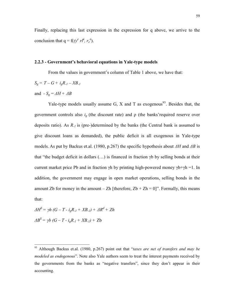
59

Finally, replacing this last expression in the expression for q above, we arrive to the

conclusion that q = f((ye rle, ree).

2.2.3 - Government’s behavioral equations in Yale-type models

From the values in government’s column of Table 1 above, we have that:

Sg = T – G + igR-1 – XB-1

and - Sg = ΔH + ΔB

Yale-type models usually assume G, X and T as exogenous93. Besides that, the

government controls also ig (the discount rate) and ρ (the banks’required reserve over

deposits ratio). As R-1 is (pre-)determined by the banks (the Central bank is assumed to

give discount loans as demanded), the public deficit is all exogenous in Yale-type

models. As put by Backus et.al. (1980, p.267) the specific hypothesis about ΔH and ΔB is

that “the budget deficit in dollars (…) is financed in fraction γb by selling bonds at their

current market price Pb and in fraction γh by printing high-powered money γb+γh =1. In

addition, the government may engage in open market operations, selling bonds in the

amount Zb for money in the amount – Zh [therefore, Zb + Zh = 0]”. Formally, this means

that:

ΔHS = γh (G – T - igR-1 + XB-1) + ΔRd + Zh

ΔBS = γb (G – T - igR-1 + XB-1) + Zb

93 Although Backus et.al. (1980, p.267) point out that “taxes are net of transfers and may be

modeled as endogenous”. Note also Yale authors seem to treat the interest payments received by

the governments from the banks as “negative transfers”, since they don’t appear in their

accounting.

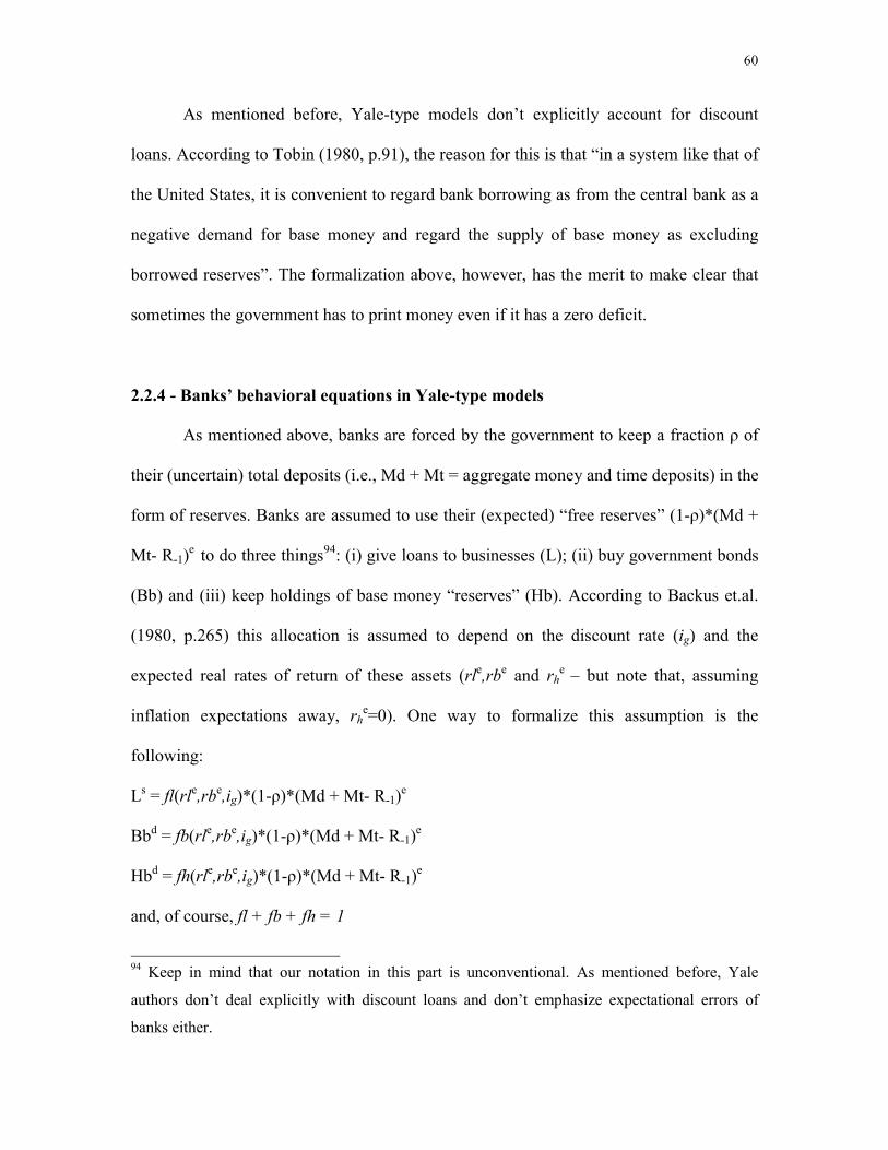
60

As mentioned before, Yale-type models don’t explicitly account for discount

loans. According to Tobin (1980, p.91), the reason for this is that “in a system like that of

the United States, it is convenient to regard bank borrowing as from the central bank as a

negative demand for base money and regard the supply of base money as excluding

borrowed reserves”. The formalization above, however, has the merit to make clear that

sometimes the government has to print money even if it has a zero deficit.

2.2.4 - Banks’ behavioral equations in Yale-type models

As mentioned above, banks are forced by the government to keep a fraction ρ of

their (uncertain) total deposits (i.e., Md + Mt = aggregate money and time deposits) in the

form of reserves. Banks are assumed to use their (expected) “free reserves” (1-ρ)*(Md +

Mt- R-1)e to do three things94: (i) give loans to businesses (L); (ii) buy government bonds

(Bb) and (iii) keep holdings of base money “reserves” (Hb). According to Backus et.al.

(1980, p.265) this allocation is assumed to depend on the discount rate (ig) and the

expected real rates of return of these assets (rle,rbe and rhe – but note that, assuming

inflation expectations away, rhe=0). One way to formalize this assumption is the

following:

Ls = fl(rle,rbe,ig)*(1-ρ)*(Md + Mt- R-1)e

Bbd = fb(rle,rbe,ig)*(1-ρ)*(Md + Mt- R-1)e

Hbd = fh(rle,rbe,ig)*(1-ρ)*(Md + Mt- R-1)e

and, of course, fl + fb + fh = 1

94 Keep in mind that our notation in this part is unconventional. As mentioned before, Yale

authors don’t deal explicitly with discount loans and don’t emphasize expectational errors of

banks either.

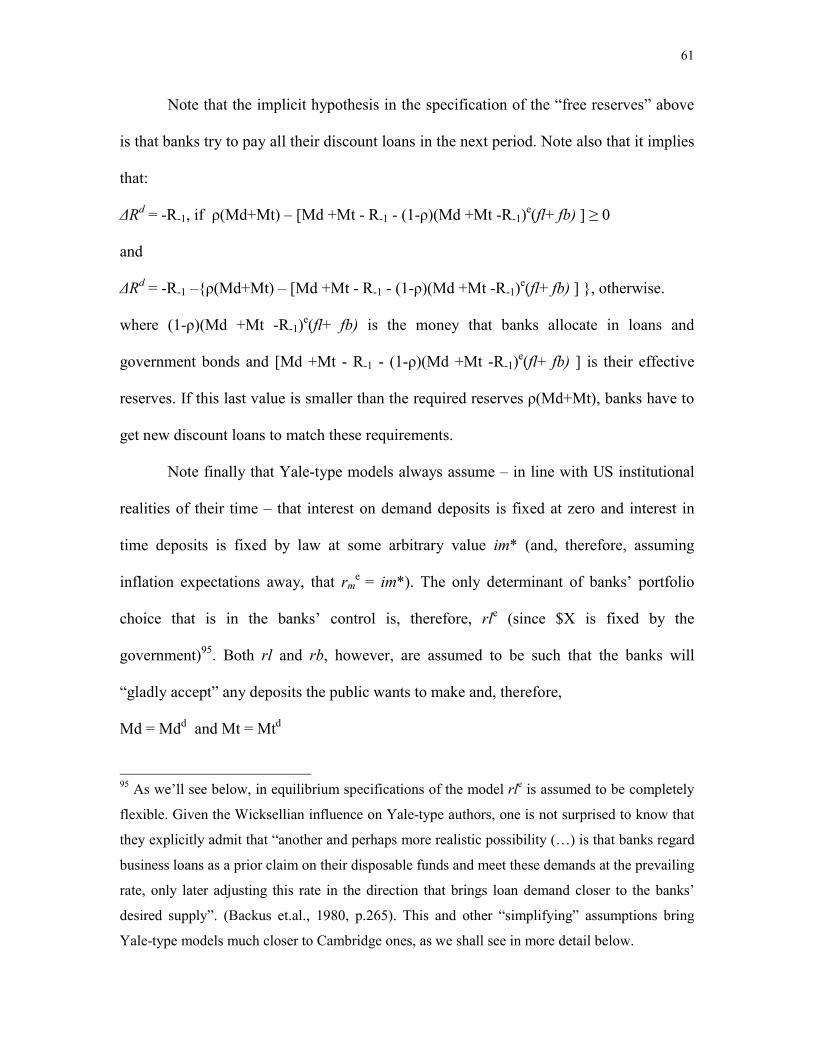
61

Note that the implicit hypothesis in the specification of the “free reserves” above

is that banks try to pay all their discount loans in the next period. Note also that it implies

that:

ΔRd = -R-1, if ρ(Md+Mt) – [Md +Mt - R-1 - (1-ρ)(Md +Mt -R-1)e(fl+ fb) ] ≥ 0

and

ΔRd = -R-1 –{ρ(Md+Mt) – [Md +Mt - R-1 - (1-ρ)(Md +Mt -R-1)e(fl+ fb) ] }, otherwise.

where (1-ρ)(Md +Mt -R-1)e(fl+ fb) is the money that banks allocate in loans and

government bonds and [Md +Mt - R-1 - (1-ρ)(Md +Mt -R-1)e(fl+ fb) ] is their effective

reserves. If this last value is smaller than the required reserves ρ(Md+Mt), banks have to

get new discount loans to match these requirements.

Note finally that Yale-type models always assume – in line with US institutional

realities of their time – that interest on demand deposits is fixed at zero and interest in

time deposits is fixed by law at some arbitrary value im* (and, therefore, assuming

inflation expectations away, that rme = im*). The only determinant of banks’ portfolio

choice that is in the banks’ control is, therefore, rle (since $X is fixed by the

government)95. Both rl and rb, however, are assumed to be such that the banks will

“gladly accept” any deposits the public wants to make and, therefore,

Md = Mdd and Mt = Mtd

95 As we’ll see below, in equilibrium specifications of the model rle is assumed to be completely

flexible. Given the Wicksellian influence on Yale-type authors, one is not surprised to know that

they explicitly admit that “another and perhaps more realistic possibility (…) is that banks regard

business loans as a prior claim on their disposable funds and meet these demands at the prevailing

rate, only later adjusting this rate in the direction that brings loan demand closer to the banks’

desired supply”. (Backus et.al., 1980, p.265). This and other “simplifying” assumptions bring

Yale-type models much closer to Cambridge ones, as we shall see in more detail below.

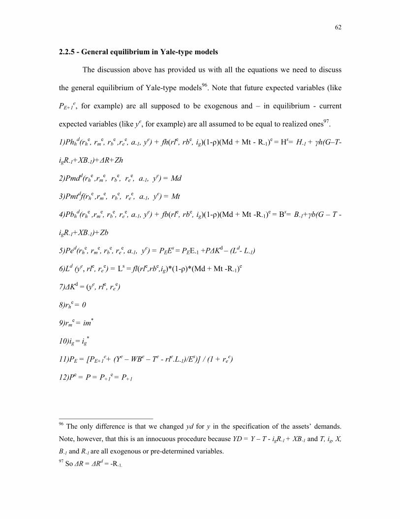
62

2.2.5 - General equilibrium in Yale-type models

The discussion above has provided us with all the equations we need to discuss

the general equilibrium of Yale-type models96. Note that future expected variables (like

PE+1e, for example) are all supposed to be exogenous and – in equilibrium - current

expected variables (like ye, for example) are all assumed to be equal to realized ones97.

1)Phhd(rh

e, rme, rb

e ,ree, a-1, ye) + fh(rle, rbe, ig)(1-ρ)(Md + Mt - R-1)e = Hs= H-1 + γh(G–T-

igR-1+XB-1)+ΔR+Zh

2)Pmdd(rhe ,rm

e, rbe, re

e, a-1, ye) = Md

3)Pmtdf(rhe ,rm

e, rbe, re

e, a-1, ye) = Mt

4)Pbhd(rh

e ,rme, rb

e, ree, a-1, ye) + fb(rle, rbe, ig)(1-ρ)(Md + Mt -R-1)e = Bs= B-1+γb(G – T -

igR-1+XB-1)+Zb

5)Ped(rhe, rm

e, rbe, re

e, a-1, ye) = PEEs = PEE-1 +PΔKd – (Ld- L-1)

6)Ld (ye, rle, ree) = Ls = fl(rle,rbe,ig)*(1-ρ)*(Md + Mt -R-1)e

7)ΔKd = (ye, rle, ree)

8)rhe = 0

9)rme = im*

10)ig = ig*

11)PE = [PE+1e+ (Ye – WBe – Te - rle.L-1)/Es)] / (1 + re

e)

12)Pe = P = P+1e = P+1

96 The only difference is that we changed yd for y in the specification of the assets’ demands.

Note, however, that this is an innocuous procedure because YD = Y – T - igR-1 + XB-1 and T, ig, X,

B-1 and R-1 are all exogenous or pre-determined variables. 97 So ΔR = ΔRd = -R-1.

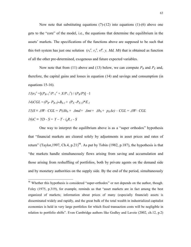
63

Now note that substituting equations (7)-(12) into equations (1)-(6) above one

gets to the “core” of the model, i.e., the equations that determine the equilibrium in the

assets’ markets. The specifications of the functions above are supposed to be such that

this 6x6 system has just one solution (rbe, re

e, rle, y, Md, Mt) that is obtained as function

of all the other pre-determined, exogenous and future expected variables.

Now note that from (11) above and (13) below, we can compute PB and PE and,

therefore, the capital gains and losses in equation (14) and savings and consumption (in

equations 15-16).

13)rbe =[(PB+1

e/P+1e + X/P+1

e) / (PB/P)] –1

14)CGL =(PB- PB-1)*Bh-1 + (PE -PE-1)*E-1

15)S ≡ ΔW– CGL = P(Δhh + Δmd + Δmt + Δbh + pEΔe) – CGL = ΔW– CGL

16)C ≡ YD - S = Y – T - igR-1 - S

One way to interpret the equilibrium above is as a “super orthodox” hypothesis

that “financial markets are cleared solely by adjustments in asset prices and rates of

return” (Taylor,1997, Ch.4, p.21)98. As put by Tobin (1982, p.187), the hypothesis is that

“the markets handle simultaneously flows arising from saving and accumulation and

those arising from reshuffling of portfolios, both by private agents on the demand side

and by monetary authorities on the supply side. By the end of the period, simultaneously

98 Whether this hypothesis is considered “super-orthodox” or not depends on the author, though.

Foley (1975, p.319), for example, reminds us that “asset markets are in fact among the best

organized of markets; information about prices of many (especially financial) assets is

disseminated widely and rapidly, and the great bulk of the total wealth in industrialized capitalist

economies is held in very large portfolios for which fixed transaction costs will be negligible in

relation to portfolio shifts”. Even Cambridge authors like Godley and Lavoie (2002, ch.12, p.2)

64

with the determination of asset prices for the period, these market participants have the

stocks of assets and of total wealth they desire at this time at the prevailing prices”.

Therefore, the general equilibrium modeled above is not simply an equilibrium of

stocks99 because it implies the flow equilibria of the economy as well. In particular, the

equilibria in the assets’ markets take in full consideration all major “flows” of the

economy (i.e., income, investment and savings/consumption), which together with the

exogenous amount of government expenditures determine the (keynesian, flow)

equilibrium in the goods’ market. Yale-type models can be seen, therefore, as general

(stock-flow) equilibrium ones.

2.2.6 - Disequilibrium and hierarchical decisions in Yale-type models

Yale authors are, however, far more heterodox than they seem. First, they clearly

admit that the general equilibrium stated above “strains credibility” (as put by Tobin,

1982, p.189). Second, they recognize that it’s often desirable to work with simpler

specifications (based on the notion of “hierarchical decisions”) of the behavioral

equations above. In what follows, we discuss first the disequilibrium specifications and

then (very briefly) the “hierarchical decisions” as they appear in Yale-type models.

As put by Brainard and Tobin (1968, p.105), “no one seriously believes that either

the economy as a whole or its financial subsector is continuously in equilibrium. (…)

Consequently analysts and policy-makers can hope to receive no more than limited

guidance from comparative static analyses of the full effects of “changing” exogenous

have recently worked with “markets for financial assets that clear instantaneously and all the

time” 99 Although it surely is a “stock” equilibrium in Foley’s (1975) sense of the term.

65

variables, including the instruments of policy. They need to know also the laws

governing the system in disequilibrium. (…) We are pleading in short for a general

disequilibrium framework for the dynamics of adjustment to a general equilibrium

system”. Of course, as Brainard and Tobin (1968, p.105) promptly recognize, there are

non-trivial problems associated with disequilibrium specifications. First, “(…) there are

many dynamic specifications that have the same static equilibrium (…) [and] economic

theory, (…) has almost nothing to say on mechanisms of adjustment”. Second, despite all

the advancements of econometric theory in the last 30 years, Brainard and Tobin are still

right to point out that “it’s precisely in the estimation of lag structures and autoregressive

effects that statistical and econometric techniques encounter greatest difficulties”.

Be that as it may, Yale-type authors always tried to deal with the disequilibrium

dynamics of their models with the use of generalized versions of the familiar “partial

adjustment” dynamic specification100. The basic hypothesis (for households) is presented

in Backus et.al. (1980, p.275) as follows:

Δanx1 = Enxn [a* – a -1]nx1 + Fnxp (S – Se)px1 + Gnxq z qx1

where, “a” is again the vector of (the “n”, = 5 in our case) households’ financial assets

(the superscript “*” denotes the “long run equilibrium” given the current effective

(expected) real rates of return and flow of disposable income), S–Se is the vector of the

“p” “sources of unanticipated changes in disposable assets (such as unplanned savings or

capital gains)”, z is the vector of the “q” variables that are supposed to “influence

adjustment behavior directly” and E, F and G are matrixes with the relevant coefficients.

100 Also used by Cambridge authors, as we’ll see below.

66

Although our purpose here is not to present a complete disequilibrium

specification of the model presented in the previous sections, it’s important to spend

some time discussing the qualitative implications of the equation above. As put by

Brainard and Tobin (1968, p.106), the first expression in the right hand side of the

equation above means that “the deviation of a variable from its “desired level”(…) is

diminished by a certain proportion at each time”, with special attention to the fact that

“the adjustment of any one asset holding depends not only on its own deviation but also

on the deviation of the other assets. The public might have exactly the right amount of

demand deposits and yet change this holding in the course of adjusting other holdings to

their desired levels”. So all the first expression in the right hand side of the expression

means is that the changes in the holdings of any given asset (say, Δbh) is assumed to be a

linear function not only of the deviation of the holdings of this asset “from its desired

level” (say, bh*

- bh-1) but also on the deviations of the holdings of the other assets as well

[i.e., (hh*- hh-1), (md*-md-1), (mt*-mt-1) and (e*-eh-1)].

The second and third terms of the right hand side of the “generalized” partial

adjustment mechanism used above say similar things with respect to both the unexpected

sources of resources and other variables that affect the adjustment process. To illustrate

the point let’s assume that the households had underestimated their disposable income

(so, yd – yde >0) and their capital gains in equity [so (PE - PEe)*E-1 > 0] and no variable

affects the adjustment process directly. In this case, the change in any given asset “ai”

would be:

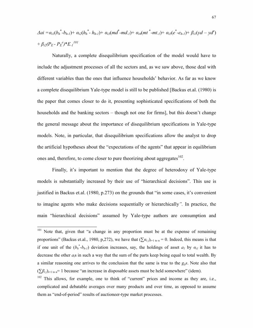
67

Δai =αi1(bh*-bh-1)+ αi2(hh

*- hh-1)+ αi3(md*-md-1)+ αi4(mt *-mt-1)+ αi5(e*-eh-1)+ βi1(yd – yde)

+ βi2(PE - PEe)*E-1

101

Naturally, a complete disequilibrium specification of the model would have to

include the adjustment processes of all the sectors and, as we saw above, those deal with

different variables than the ones that influence households’ behavior. As far as we know

a complete disequilibrium Yale-type model is still to be published [Backus et.al. (1980) is

the paper that comes closer to do it, presenting sophisticated specifications of both the

households and the banking sectors – though not one for firms], but this doesn’t change

the general message about the importance of disequilibrium specifications in Yale-type

models. Note, in particular, that disequilibrium specifications allow the analyst to drop

the artificial hypotheses about the “expectations of the agents” that appear in equilibrium

ones and, therefore, to come closer to pure theorizing about aggregates102.

Finally, it’s important to mention that the degree of heterodoxy of Yale-type

models is substantially increased by their use of “hierarchical decisions”. This use is

justified in Backus et.al. (1980, p.273) on the grounds that “in some cases, it’s convenient

to imagine agents who make decisions sequentially or hierarchically”. In practice, the

main “hierarchical decisions” assumed by Yale-type authors are consumption and

101 Note that, given that “a change in any proportion must be at the expense of remaining

proportions” (Backus et.al., 1980, p,272), we have that (∑αi j)i=1 to n = 0. Indeed, this means is that

if one unit of the (bh*-bh-1) deviation increases, say, the holdings of asset a1 by αi1 it has to

decrease the other ais in such a way that the sum of the parts keep being equal to total wealth. By

a similar reasoning one arrives to the conclusion that the same is true to the gijs. Note also that

(∑βi j)i=1 to n= 1 because “an increase in disposable assets must be held somewhere” (idem). 102 This allows, for example, one to think of “current” prices and income as they are, i.e.,

complicated and debatable averages over many products and over time, as opposed to assume

them as “end-of-period” results of auctioneer-type market processes.

68

investment decisions103. Consumption is often assumed, a la Modigliani, to depend only

on currently disposable income and the total stock of wealth (therefore being

“hierarchically superior” to households’ decisions on the allocation of their wealth).

Investment, by its turn, is assumed to be “hierarchically superior” to financial decisions.

As the authors recognize, these hypotheses are in sharp contrast to neoclassical

microeconomics104. As we’ll see below, they also bring Yale-type models much closer to

Cambridge ones than otherwise.

2.2.7 - Yale-type models: A possible summary

As mentioned before, there are several versions of Yale-type models and none of

them is exactly equal to ours (that was chosen to make the comparison with Cambridge

authors easier). They differ in emphasis, level of abstraction and aggregation but all of

them emphasize a common set of issues. First, all of them (since the seminal 1968 paper)

specify wealth demand functions (that – at least since 1978105 - are assumed to be

“integrated” with the savings decisions of households) and assume that the desired

allocation of this wealth depends on the relative real rates of return of the various

financial assets of the economy. Second, all of them assume that financial markets are

driven by a tendency toward a complete stock (of financial wealth) equilibrium, that takes

103 And possibly also the loan decisions of banks. See footnote 94 above. 104 As they put it themselves (p.273), “although [neoclassical] theory tells us that separations of

this type are legitimate only under rather strong assumptions, there’s often a compelling need for

plausible rough approximations in empirical work”. Indeed, “separations of this type” are much

closer to post-Keynesian models than to neoclassical ones. See Lavoie (1992, ch.2) for more on

this issue.

69

fully into consideration the flow (i.e., consumption/savings and investment) decisions of

the agents and, therefore, implies also the usual Keynesian flow equilibrium in the goods’

market (or the “real economy”, as they portray it). Third, and related to the second, all of

them assume that investment is determined (or, at least heavily affected) by q. Fourth, all

of them deal with these “crucial interdependences” between financial markets and the

real economy (in principle, at least) with the use of stock-flow consistent accounting

frameworks in which, to use Godley’s (1996, p.7) words, “there are no “black holes”-

every flow comes from somewhere and goes somewhere”. This accounting framework is,

then, “brought to life” (at least in the theoretical versions of the model) with explicit

general (dis)equilibrium hypothesis of the “everything depend on everything else” kind.

Theoretical Yale-type models are completely general in this sense106. They are not

general, however, in the sense that they don’t deal explicitly with the “production and

pricing” decision of firms (although they could conceivably be extended to do it) and

their treatment of the financial decisions of firms (based on the Modigliani-Miller

theorem) is less than satisfactory.

2.3 - A (“New”) “Cambridge-type” closure

As Cambridge-type SFC modeling has a long history and has changed relatively

more than its Yale counterpart, we chose to discuss it in two sections. In this one we’ll

focus on the first Cambridge-type models, i.e., those written in the seventies and eighties

105 Tobin (1980) presents a published version of his 1978 Yrjo Jahnsson Lectures, in which he

states this point very clearly. 106 Although, as we mentioned before, empirical versions of the model often replace these general

specifications by simpler ones, based on the hypothesis of “hierarchical decision making”.

70

by Wynne Godley and his team at the Department of Applied Economics, Cambridge. As

most of this early Cambridge-type SFC theorizing (baptized as “New Cambridge view”

by journalists) aimed to influence the public debate about macroeconomic policy-making

in the United Kingdom it’s not surprising that it dealt basically with applied open-

economy models. These models were, however, based on a very distinctive theoretical

view according to which “the tendency of the [macroeconomic] system as a whole is

governed by stock-flow norms rather than (…) equilibrium (or disequilibrium) conditions

postulated by neoclassical theory” (Godley, 1999a, p.396). This view was carefully

presented in a textbook by Godley and Cripps (1983 –from now on G&C)107, from which

the present section will draw heavily.

2.3.1 - The level of aggregation in early Cambridge-type models

One distinguishing feature of the Cambridge approach is its emphasis on direct

theorizing about aggregates108. Indeed, as put by G&C (1983, p.18, emphasis in the

107A book prepared especially for this task. Indeed, in April 1980, the Cambridge Economic

Policy Group (CEPG) acknowledged that “(…) our publications have fallen well short of a

comprehensive statement of our views (…). There is no satisfactory solution [to this problem]

other than write, in due course, our own textbook” (CEPG, 1980, p.35). Godley and Cripps

(1983) is precisely the textbook they were talking about. 108 Again, the difference between Cambridge and Yale is not as large as one would think. Tobin

(1982, p.173-174) explicitly recognizes that Yale-type models are “only loosely linked to

optimizing behavior of individual agents. Following an older tradition, economy-wide structural

equations are an amalgam of individual behavior and aggregation across a multitude of diverse

individuals”. This view is not completely outdated either, since it is at the very core of the

influential “LSE approach” to macroeconometrics. As put by Hendry (in Backhouse and Salanti,

“Macroeconomics in the Real World” OUP, 2000, p.156) “the theoretical models underlying

what I am doing are much more like the hydrologist’s theoretical model. It is simply

71

original) “since human behaviour is so varied, our objective will be to establish principles

of analysis which capitalize on adding-up constraints so as to confine behavioural

processes to a relatively small number of variables, each of which can then be object of

empirical study. The smaller the number of behavioural variables which govern how the

system must function in the view of the logical constraints, the more powerful will be our

theory as a model of organizing and interpreting data”. This emphasis implies that the

level of aggregation of any New Cambridge-type model that aims to describe the

dynamics of a real economy in historical time is in principle an open issue (though

subject to the minimum requirement of separating the public, the private and the external

sectors of the economy)109. The New Cambridge-type procedure, to put it briefly, appears

to be to choose the level of aggregation in which the stronger empirical regularities can

unimaginable where hydrology would be today if hydrologists had insisted on working out the

theory of turbulence from quantum dynamics. They wouldn’t have made one iota of contribution

to understanding it because it is a system property and it is enormously complicated how

turbulence behaves, how waves behave, how they propagate, etc. They have theories about these

things that are macro theories. They are not based on individual agents. I don’t work with that

kind of model [i.e., the mainstream representative agent ones] because I simply don’t know how

one agent trades with itself in the stock market, and forms all these expectations and carries out

intertemporal optimization, etc, etc. I simply don’t see how it is done and I don’t know how to do

it with a hundred million heterogeneous agents (…)”. Finally, note that the bulk of the

methodological literature is also critical of the “representative agent” hypothesis. For one among

many methodological critiques of models based on this hypothesis, see Hoover (2001, chapter 5). 109 These points are explicitly made, for example, in G&C’s methodological chapter (1983, p.42-

43) and in the discussion of the relevant concept of wealth to be introduced in a Cambridge-type

model (see G&C, p.265).

72

be found110 about the minimum possible number of behavioral hypotheses (generally

about stock-flow ratios).

For this particular reason, early Cambridge-type models usually worked with the

notion of the “private sector as a whole” (i.e., the aggregation of households, banks and

firms in Table 1 above). Indeed, as put by Godley and Fetherston (1978, p.34), “the

explicit hypothesis associated with the term “New Cambridge” is that virtually all

disposable income of the private sector as a whole will be spent on goods and services

with a fairly short lag. In our econometric work (…) a persistent feature of the results is

that with the total private expenditure [i.e., C+PΔK in Table 1 above] as the dependent

variable, the coefficients on current and (one year) lagged nominal private disposable

income sum to very nearly unit”. Note that this aggregation had the further advantage to

allow Cambridge economists to avoid complicated matters related with firms’ financial

decisions. As summarized by Cripps and Godley (1976, p.336), “given the well-known

difficulty of modeling the corporate sector there is an advantage in aggregation provided

the overall relationship is empirically robust”.

To make a long story short, the “New Cambridge hypothesis” generated a good

deal of controversy (especially in the UK111) but wasn’t well accepted mainly because the

bulk of the economics profession at the time considered “the aggregation of personal

consumption with corporate investment (…) inadmissible in principle” (Anyadike-Danes,

1982, p.33). Be that as it may, what is relevant for us here is to note that the “New

110 At least this is what one can infer from the discussion mentioned in the previous footnote (see

G&C, p.266). 111 See, for details, Vines (1976), Cuthbertson (1979) and McCallum and Vines (1981).

73

Cambridge” model can be seen as a (formally) simplified version of the Yale-type model

discussed in section 2.2 above. That’s our topic in the following sections.

2.3.2 - The constant stock (of private wealth)-flow (of private disposable income)

hypothesis

The crucial hypothesis of New Cambridge models is that the private sector as a

whole has a relatively constant desired stock(of wealth)-flow(of disposable income) ratio.

If, for example, this desired stock-flow ratio is, say, ¾ and the flow of disposable income

is 100 per period, then the desired stock of wealth would be 75. The potential problems of

this hypothesis (or, as called by G&C, this “behavioural axiom”) are acknowledged by

G&C (p.60) but the authors give no solution to them other than stating (p.42) that “the

formal status of the axiom is akin to that of an exogenous variable. It’s something that the

model itself cannot explain. We admit without reservation that if stock-flow norms were

to move about too wildly most of the theory (…) would be rendered useless”. Formally,

the “axiom” means that:

W* = αYD, where α is the exogenous stock-flow, W* is the households’ desired stock of

wealth112 and YD is households’ disposable income.

Before we discuss the implications of this hypothesis, it’s probably illuminating to

compare it with the Yale view on this matter. As we saw in section 2.2.1 above, in Yale-

type models the “desired long run wealth target” of households is assumed to be a (not

specified, but probably complicated) function of (i)the real rates of return of financial

assets, (ii)current disposable income and (iii)other factors like income distribution, age

74

structure, the stock of human capital and expected incomes (that are implicitly taken as

exogenous in the analysis). In other words, in Yale-type models the desired stock (of

wealth)-flow (of disposable income) depends in a very complicated and unspecified way

on many endogenous and (sometimes implicit) exogenous variables. In such a

circumstance, it seems reasonable – as an intermediate step, at least – to treat it as an

exogenous variable113. Indeed, as Solow (2000, p.98, emphasis in the original) reminds us

“to treat a parameter as exogenous is not the same thing as to treat it as a permanent

constant or as inexplicable. The rate of population growth [for example] was (…)

generally treated as exogenous in old growth theory. But everyone knew that fertility and

mortality change from time to time (…). Moreover everyone knew that sometimes one

can understand, especially after the fact, why population growth is now faster or slower

than what used to be. What is lacking [when one treats something as exogenous] is a

good, systematic, generally acceptable theory [to explain this thing]”114.

Of course, one must keep in mind that while the Yale-type assumption concerns

the households’ sector only, the (“New”) Cambridge assumption is about the private

sector as a whole. But note that, given the Yale-type assumptions about the validity of

the Modigliani-Miller theorem for non-bank businesses (and the simplifying assumptions

it makes about banks), households’ (net) wealth and disposable income are exactly equal

112 What exactly must enter in the concept of wealth is a non-trivial issue, as we’ll discuss in more

detail below. 113 But see the discussion on section 2.3.6 below. 114 Note also that Cambridge authors explicitly recognized the possibility of “perturbations” on

their postulated asset/income norm (see discussion below) but argued that it “enables so much to

be explained with so little that it serves as a very powerful organizing principle even if the norm

has a time-trend or is moderately unstable” (Godley, 1983, p.140).

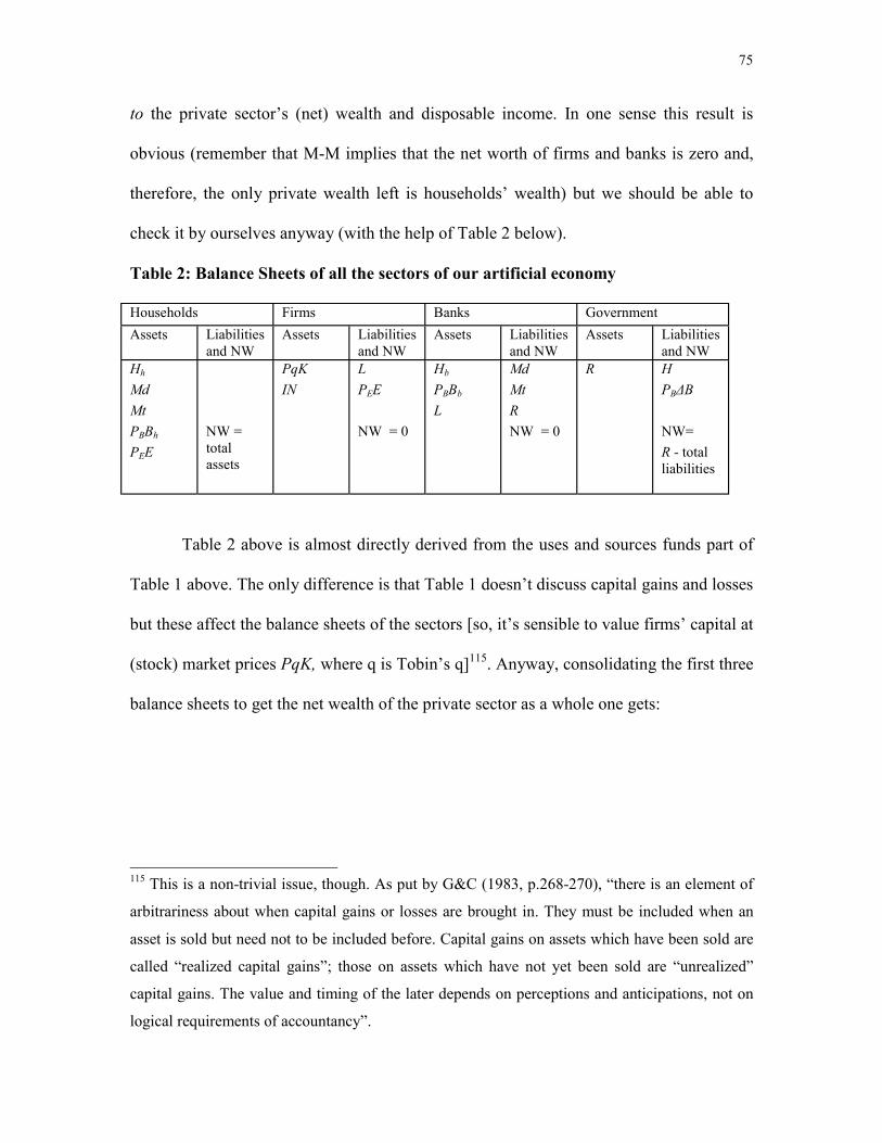
75

to the private sector’s (net) wealth and disposable income. In one sense this result is

obvious (remember that M-M implies that the net worth of firms and banks is zero and,

therefore, the only private wealth left is households’ wealth) but we should be able to

check it by ourselves anyway (with the help of Table 2 below).

Table 2: Balance Sheets of all the sectors of our artificial economy

Households Firms Banks Government Assets Liabilities

and NW Assets Liabilities

and NW Assets Liabilities

and NW Assets Liabilities

and NW Hh Md Mt PBBh

PEE

NW = total assets

PqK IN

L PEE NW = 0

Hb PBBb

L

Md Mt R NW = 0

R

H PBΔB

NW= R - total liabilities

Table 2 above is almost directly derived from the uses and sources funds part of

Table 1 above. The only difference is that Table 1 doesn’t discuss capital gains and losses

but these affect the balance sheets of the sectors [so, it’s sensible to value firms’ capital at

(stock) market prices PqK, where q is Tobin’s q]115. Anyway, consolidating the first three

balance sheets to get the net wealth of the private sector as a whole one gets:

115 This is a non-trivial issue, though. As put by G&C (1983, p.268-270), “there is an element of

arbitrariness about when capital gains or losses are brought in. They must be included when an

asset is sold but need not to be included before. Capital gains on assets which have been sold are

called “realized capital gains”; those on assets which have not yet been sold are “unrealized”

capital gains. The value and timing of the later depends on perceptions and anticipations, not on

logical requirements of accountancy”.

76

NWpriv=Hh +Md + Mt + PBBh +PEE + PqK + IN+ Hb +PBBb +L – L - PEE– Md – Mt -R

or, equivalently,

NWpriv = Hh + PBBh + PqK + IN + Hb + PBBb -R (= H + PBB + PqK + IN -R)

But now note that from the balance sheet of firms we know that PqK + IN = L + PEE.

Replacing this result above we get:

NWpriv = Hh + PBBh + PEE + L + Hb + PBBb -R (= H + PBB + PEE + L - R)

To get the result we stated above all one needs to do now is to note that from the balance

sheet of banks we have that L + Hb + PBBb= Md + Mt +R and, therefore,

NWpriv = Hh + PBBh + PEE +Md + Mt

In other words, one possible way to think about the “New Cambridge axiom” above is as

a simplified, easy to handle, version of its complicated Yale counterpart116.

Note also that the “New Cambridge axiom” implies a (stationary) steady-state in

which the stock of wealth and income are such that the marginal propensity to consume is

equal to one117. While this may be interpreted as a private sector’s “Say’s Law”118, one

must remember that (i) to argue in favor of a steady-state private sector’s “Say’s Law” is

116 A similar point was made by Coutts and Godley (1984, p.28). Note also that Yale authors

implicitly recognize this when using Modigliani-type consumption functions in simplified

versions of their models (based on hierarchical decisions). See next page for more on the issue.

Note, finally, that both schools might differ on the relevant concept of wealth used and

Cambridge authors don’t base their conclusions on the M-M theorem. See discussion on section

2.3.5. 117 And, possibly, also a steady-growth state in which this is not true. See the third essay of this

dissertation for more details. 118 Especially if the adjustment to this stationary steady-state is quick (as originally assumed by

New Cambridge authors – see section 2.3.7). This point was brought to my attention in a private

communication with Franklin Serrano

77

very different than to argue in favor of “Say’s Law”119 and (ii) it seems difficult to deny

that “households vary greatly (…) from extremely liquidity-constrained consumers who

live hand-to-mouth and spend quickly any cash receipts, to lords of dynasties who save

all extra income for descendents” (Tobin, 1982, p.185-186). But if this second point is

true, i.e., if the consumption function of households depend – a la Modigliani – on both

their current disposable income and stock of wealth120, then the existence of the “New

Cambridge” steady state is in general guaranteed (as stressed by Coutts and Godley,

1984, p.28). To see this last point, note that in the steady-state, ΔW=0 (because, wealth is

already at its desired level, W*) and, therefore, C=YD121. So, given that

C = f (YD, W-1), we would have that

YD = f (YD, W*) and, assuming that “f” is well behaved, this equality allows us to find

α = W*/YD122

119 In modern capitalist economies government and foreign (net) expenditures are too important to

be neglected, so the point is supposed to be more serious to the analysis of the early stages of

capitalism. Note, however, that the private sector’s marginal propensity to consume is equal (or

very close) to one either when the stock of wealth is already at its desired level or when income is

so small that has to be completely used with subsistence consumption. As put by Taylor (1997,

ch.2) this last reason (and not, of course, the first) may explain why the classical economists of

18th and 19th century considered Say’s Law a good approximation of reality. 120 As, by the way, is implied by models that deal with “autonomous” consumption by nationals

that neither work for the government nor are capitalists. 121 Net investment and changes in debt are assumed to be zero in such a steady-state. This implies

that either depreciation is being neglected or gross investment is financed entirely by purchases of

equity by households and, therefore, C+I = YD. In this case, of course, the derivation above must

be changed to assume that C+I = f (YD, W-1). 122 The linear example is trivial. If C = aYD + bW-1 , then α = (1-a)/b

78

2.3.3 - Production decisions and their financing in New Cambridge-type models

Besides the exogenous stock (of wealth)-flow (of private disposable income) ratio

hypothesis, another trademark of Cambridge-type SFC modeling is its emphasis on the

importance of taking explicitly into consideration that (i) “production and distribution

take time and future is always uncertain” (Godley,1999, p.394); (ii)“entrepreneurs have

to pay out money for working [and fixed] capital to keep production going in advance of

receiving money from the sales of goods” (G&C, p.66) and, therefore, (iii) “finance must

be forthcoming if the private sector is to grow; hence the need for a representation of

commercial banking system, debt and inside money” (Anyadike-Danes et.al., 1987, p.10-

11). This Cambridge emphasis on the financing of firms’ production is in sharp contrast

with the Yale-type story, which, as we saw in section 2.2.2 above, completely neglects

these issues123.

The New Cambridge story about production decisions by firms is pretty

conventional. In the beginning of the production period firms are assumed to formulate

expectations about the quantities they will be able to sell at given “normal” prices and

decide what to produce based on these expectations “plus the change in inventories they

want to bring about” (Godley, 1996, p.14). Note that, as much as their Yale counterparts

(see footnote 86 above), early Cambridge models didn’t pay too much attention to

expectation errors by firms, always assuming that they have sufficient foresight or

flexibility to adjust their stock of inventories to a given desired proportion of some

123 An explicit Cambridge critique to the lack of attention given by Yale authors to production

decisions by firms can be found in Anyadike-Danes et.al. (1987, p.10-11), according to whom,

this is one of a “number of respects in which the Tobinesque tradition can usefully be further

developed”.

79

relevant flow124. New Cambridge authors have also worked, again as much as their Yale

counterparts, with simplified models in which the change in inventories is zero or fixed

(see for example, G&C, chapters 13 and 14). The practical difference is that while Yale

authors worked - in more sophisticated models – with the hypothesis that ΔIN =f(q), New

Cambridge authors assumed, say, that ΔIN =γFE =γ(C+G+PΔK) or ΔIN =γYD

(depending on which relation happened to be more reliable in practice). To keep the

algebra simple, we’ll assume in the next sections that inventory accumulation is

exogenous, though125

As we mentioned before, things get really different between the two schools when

it comes to explicitly theorizing about how firms finance production. The New

Cambridge hypothesis (heavily influenced by Kaldorian ideas) is that firms finance all

necessary advancements through borrowing and, therefore, capitalists “can spend all their

(net) profits” and “yet remain solvent because their debt is matched by realizable assets

[i.e, their inventories]” (G&C, p.72). To make the content of this assumption clear let’s

assume (as in G&C, ch.4) that the total cost of production of a firm is 100 and that it

marks up each unit by 10%. Assuming also that the firm correctly forecasts its final

124 In G&C (1983, p.108) the relevant flow is the flow of past final sales, while in Godley (1983,

p.147) it is the flow of disposable income. These changes are probably based on the Cambridge

emphasis on using empirical regularities discovered at the macro level, as discussed above. Note

also that New Cambridge authors give a lot of importance to inventory-dynamics. As put by G&C

(1983, p.86) it is important to discuss the consequences of treating financed inventories as

endogenous (...) [because] small changes in the desired ratio of inventories to income could alter

the whole dynamic of income-expenditure flows (...)”. 125 See the third essay of this dissertation for a New Cambridge model with inventory dynamics.

As we’ll discuss below, current Godley-type papers invariably assume a desired stock (of

inventories)-flow (of final sales) and deal with firms’ expectation errors explicitly.

80

demand (and, therefore, its final sales), it is clear that the total sales revenue of the firms

is 110. If it had borrowed 100 to finance production, the firm would be able to pay the

bank (in this example we are assuming, for simplicity reasons only, that the interest rate

is 0%) and get 10 as a “profit”126. As the firm, by assumption, can always borrow what it

needs to finance its production next period, the whole “profit” can be spent without

imposing any restriction on the level of production.

Now let’s assume that in the first period of production the firm didn’t sell

anything borrowing (100) to produce inventories to match next period’s demand. In this

case, it is clear that the firm’s debt in the end of the production period (100) is matched

by its assets (100), since the firm used the borrowed money to buy/produce the

inventories. It is also clear that in the second period, when the firm sells its previous

production and borrows (say, 100 again) to rebuild its inventories, its revenues (110)

won’t be enough to pay all its debt (100+100 = 200). However, revenues less

“profits”(110 - 10 = 100) will be big enough to avoid a further increase in the debt. The

firm will only need to increase its debt again if it needs to increase its inventories either

to prepare for an increase in sales in the future or in case of an unexpected decrease in

sales. In both cases it would need to borrow more than its current total revenue excluding

“profits”, increasing its debt as a consequence. Applying a similar reasoning, it is easy to

notice that if a firm needs to reduce its inventories, it will be decreasing its debt as a

consequence.

126Our definition of profits here is a loose one and means “what is left from what is sold after one

pays for what it did cost”. A more sophisticated definition would incorporate at least the changes

on the stock of inventories (see Godley and Cripps p.68). Yet more sophisticated definitions can

be found in Alemi and Foley (1997) and Godley (1996).

81

In other words, the assumption here is that whenever they increase (decrease)

their inventories of working capital, firms borrow (pay) from (to) banks the exact amount

required (available) to do so. Formally, ΔIN = τΔL (where, L is the firms’ stock of debt

with banks and τ is a real number such that 0 ≤ τ ≤ 1127).

2.3.4 - Government’s behavioral equations in New Cambridge models

The crucial hypotheses are two. First, the government is supposed to keep its net

income (YG= T+igR-1-XB-1, in our case) as a fixed proportion (θ) of national income.

Second, the government is supposed to choose the amount of money it will spend in

goods and services (G). In other words, the government is assumed to choose the “fiscal

stance” (G/θ) of the economy.

Other hypotheses are that: (i) the central bank is supposed to give discount loans

to banks whenever necessary and (ii) the government chooses both X (i.e., the amount of

money per bond it pays in each period to the owners of government bonds) and the

supply of bonds it will offer to the public (B) to control the price of bonds (PB) and,

therefore, their (implicit) “interest rate”. As a consequence, the composition of public

debt (in particular, the quantity of money available in the economy) is chosen by the

public exclusively.

2.3.5 - Wealth, consumption and investment in New Cambridge models

As seen in section 2.3.2 above, a crucial New Cambridge assumption is that the

private sector as a whole has a desired stock (of wealth)-flow (of disposable income) ratio

127 Remember that in our artificial economy households’ don’t get loans but firms can get loans to

82

“α”. Contrarily to what happens in Yale-type models (in which the relevant concept of

wealth is clearly defined128), however, the relevant concept of wealth is an open issue in

New Cambridge-type models. As put by G&C (p.266), “the minimum requirement of a

definition of the stock of assets in a macroeconomic model is that it should permit us to

pin down precisely the flow budgets of the private sector and the government (and, in an

open economy, the external world). (…) Beyond this the choice of definition is

essentially an empirical question, the key issue being which measure of the stock of

assets will yield the greatest behavioural regularity of stock-flow ratios”.

As transactions in assets like durable goods, equities and land are almost all

confined to the private sector (and, therefore, do not affect the budget constraints of

neither the private sector as a whole nor of the public sector and of the rest of the world),

their introduction in the relevant concept of wealth would be questionable. As put by

G&C (p.267): “If a narrow definition of the stock of assets is adopted, adjustments to

stocks of assets that have been excluded (e.g., equity and fixed capital) may perturb the

stock-flow norm and dynamics of adjustment of assets which have been included (e.g.,

money and bonds). The extent of these disturbances(…) is strictly a behavioral issue”. Of

course, one might very well find these “disturbances” to be in fact very strong. If this is

the case, according to G&C (ibid) themselves, “(…) models ought ideally to be expanded

to allow for this. There will, however, be a cost as well as a gain. For although it should

be possible to give a better representation of asset adjustments, the processes which

generate changes in stocks of assets will now include such things as rises and falls in

stock market and property values, which are themselves hard to understand and predict”.

finance investment in fixed capital as well as inventories.

83

As the passages above make clear, New Cambridge authors saw Yale’s concept of

wealth and assumptions about assets being gross substitutes in households’ portfolios as

questionable theoretical choices/empirical issues and preferred to look for (relatively)

stable stock-flow ratios in the data129. For the sake of comparison, however, we’ll assume

here that the relevant concept of wealth is the same for both schools, i.e., that the desired

stock-flow norm α applies to net private wealth as defined in section 2.3.2 above.

Formally this means that:

NW* =(Hh + PBBh + PEE +Md + Mt)* = αYD = α(1- θ)Y 130

Now note that, as much as their Yale counterparts, Cambridge authors explicitly

acknowledge that real economies are not in general in (stock-flow) equilibrium and often

use a “partial adjustment” dynamic specification in their models131. Accordingly, we’ll

assume here that:

ΔNW=Φ(NW* - NW-1) = Φ(α(1- θ)Y - NW-1) [equation 1]

128 See discussion in section 2.2.1 above. 129 As far as we know, Yale authors haven’t written about the implications of alternative concepts

of wealth. Note, in particular, that households don’t invest in their models, so durable goods

(including housing) and land are assumed away in their concept of wealth. Yale-type models

could conceivably be extended to deal with more complex definitions of wealth, though. 130 See, for example, Godley (1983, p.152) for a similar formalization. Here, however, we assume

that net wealth includes past capital gains. As put by Solow (1983, p.164, emphasis in the

original) a “problem [with the formalization in Godley (1983)] is that it define[s] ‘aggregate

financial assets’ as the sum of all past differences between disposable income and private

expenditures, a total unaffected by capital gains and losses on existing assets. The problem is that

it’s not clear why anyone should wish to achieve and maintain a fixed ratio of this total to

disposable income”.

84

where Φ is the “speed-of-adjustment parameter”132

So, again we are assuming something that is closely related to a Yale-type assumption.

Indeed, one possible way to look at the equation above is as an aggregated and simplified

version of Yale’s “general disequilibrium framework” presented in section 2.2.6 above,

one that, as Godley (1983, p.152) admits, “heroically (…) [ignores] problems associated

with the distribution of wealth within the private sector”133.

To understand how this hypothesis is used in Cambridge-type models, one first

has to note that: DΔNW = ΔGD + ΔPD + CGL -ΔR [equation 2]

where, ΔGD = G –YG = G – θY = G - T - ig R-1 + XB-1 = - Sg = ΔH + PBΔB = public

sector’s deficit (excluding capital gains or losses in public bonds)

ΔPD =PEΔE + ΔL = change in firm’s liabilities (excluding capital gains or losses in

stocks)

CGL = ΔPEE-1 + ΔPBB-1 = capital gains or losses in stocks and public bonds134

131 See, for example, G&C (1983, ch.6) or the third essay of this dissertation for Godley-type

models with a partial adjustment mechanism. See also G&C (1983, p.48, last paragraph) for a

very concise exposition of their views on steady-states and disequilibrium. 132 See G&C(1983, p.126). Most Cambridge-type models (like, for example, the ones in G&C

ch.13 and 14) assume special hypotheses about Φ to simplify the algebra (see section 3.2.4 below

for details). Here, however, we’ll keep the model as “pure” as possible. 133 Again, it’s important to emphasize that Cambridge-type models don’t rely on M-M

conclusions but on empirical regularities found at the macro level. 134 To see why equation 2 holds, note first that NW = H + PBB + PEE + L -R (see section 2.3.2

above). Therefore:

ΔNW = H + PBB + PEE + L -R – (H-1 + PB-1 B-1 + PE-1 E-1 + L-1 -R-1),

or equivalently:

ΔNW = ΔH + ΔL - ΔR +( PBB - PB-1 B-1) + (PEE– PE-1 E-1) ≡ ΔGD+ΔPD+CGL-ΔR.

85

Indeed, a simple way to find the “one-period” solution of our Cambridge-type

model is precisely to replace equation (1) above in equation (2), to get

Φ[α(1- θ)Y - NW-1]= ΔGD + ΔPD + CGL -ΔR = G – θY + ΔPD + CGL -ΔR

Or, rearranging, assuming exogenous ΔPD, ΔR and CGL (see next section) and solving

for Y:

Y=λ(G + ΔPD + CGL- ΔR + Φ NW-1)

where, λ = 1 /[θ + Φα(1- θ)]

Given the similarities between Cambridge-type models and Yale-type models it is not

surprising that we were again able to find the flow of income, without any reference to

consumption or investment135. The answer, again, is that the flow behavior of the system

is taken in full consideration in the derivation of the stock adjustment process. To find

(the aggregate of) consumption and investment, all one needs to do is to rearrange the

national income identity for a closed economy:

C + I = Y - G - ΔN136

or, using the “one period” solution for Y derived above:

C + I = λ [DPD + CGL -DR + Φ NW-1] – (1- λ)G + ΔIN

where the expression above is a version of the New Cambridge “private expenditure

function”137.

To derive the identity above is important to note that PBΔB + ΔPBB-1= PBB - PB-1 B-1 and an

equivalent result holds for equities as well. 135 As we did in section 2.2.5 above (see also the discussion in section 2.2.1). This time, however,

there’s no implication that this flow of income is an equilibrium one. 136 Keep in mind that we are simplifying things here by assuming that ΔIN is exogenous. 137 The differences of this expenditure function from, for example, the one in Godley and

Fetherston (1978, p.42) that states the quintessential “New Cambridge Hypothesis” mentioned in

86

Finally, to disaggregate between C and I, all one has to do is to use the fact that I

≡ ΔPD - ΔIN (both of which are being treated as exogenous variables here – see section

2.3.6 below).

2.3.6 - The “financial side” of the economy in New Cambridge-type models

A perennial critique of New Cambridge models (and in fact of Kaldorian

Keynesianism in general) is that they (it) “trivialize(s)” monetary policy and financial

issues138. Indeed, although one finds some interesting passages about the financial side of

the economy in the writings of New Cambridge authors139, these considerations do not

affect the formal solution of New Cambridge models140. So it seems fair to say that New

Cambridge-type models assume financial decisions of agents (including portfolio

decisions of households and banks and financing decisions of firms related to investment

in fixed capital) and their consequences (as far as the determination of interest rates and

capital gains is concerned, for example) as roughly exogenous141 – what explains the

assumptions made above. The only explicit hypotheses about these issues (as discussed in

section 2.3.1 above, are due to the particular concept of wealth and “partial adjustment”

mechanism assumed here. 138 This view is expressed, for example, by Blinder (1978, p.83). 139 All of them very close to Yale-type hypotheses. See, for example, Godley and Fetherston

(1978, p.43) and its formalization by Blinder (1978, p. 71-73) or G&C (1983, ch.8, especially

p.160-161 and also ch.13, especially p. 264-265). 140 As far as we know these insights have only been formalized in more recent papers

(particularly Godley, 1996 and 1999). See below for more on recent Cambridge-type models. 141 Two exceptions are the models in Godley and Cripps (1983, ch.7, appendix) and Godley

(1983) that assume a fixed stock (of aggregate debt of both firms and families)-flow (of private

disposable income) norm, probably based on some empirical regularity observed at the macro

level.

87

sections 2.3.3 and 2.3.4. above) are that (i) the government acts to control the interest rate

on bonds and (ii) a large part or all inventory accumulation is financed by bank loans.

The contrast of these assumptions with the Yale-type emphasis on real-financial

interdependencies is striking and was noted, for example, by Solow (1983, p.165):

“I have some sympathy with Godley’s analytical device of getting monetary policy out of the way

by assuming it to be permissive in the sense that the central bank holds the interest rate constant. But one

can hardly stop there, for both practical and analytical reasons. The modern economy generates a wide -

and changing – menu of financial assets that are imperfect substitutes for one another on both the supply

side and the demand side. There are as many interest rates as assets. A completed Keynesian model must

certainly contain a lot of portfolio theory; it will have to model asset exchanges as thoroughly as exchanges

of goods and services. This vein has been most thoroughly mined by Tobin (…). I would hope Godley could

follow suit”.

As we’ll discuss in more detail below, Godley did follow suit indeed. Note, however, that

whether the New Cambridge assumptions are too simplified or not depends on one’s

point of view. In particular, Yale-type assumptions have never been tremendously

successful empirically and it’s not clear what exactly to put in their place. As far as

capital gains are concerned, for example, most modern economists would probably agree

to treat them as exogenous. Given the lack of alternatives, the use of empirically reliable

stock-flow ratios seems less arbitrary than otherwise.

Before we continue it’s important to notice that New Cambridge authors were not

clear also about (i) the determinants of the disaggregation of private expenditure on

consumption and investment and (ii) the potential impact of changes in the interest rates

on the private sector’s desired stock (of wealth)-flow (of disposable income) norm. We’ll

finish this section commenting on these two issues, beginning by the first.

88

As we mentioned before the desired stock (of wealth)-flow(of disposable income)

ratio affects directly the aggregate of consumption and investment in New Cambridge

models. Indeed, nothing is said in these models about the disaggregation of consumption

and investment and, as put by Blinder (178, p.69) “the [New Cambridge] message may

be that any such division should not be attempted”. Whether this was or not the case, the

fact is that current Cambridge type models do disaggregate between consumption and

investment decisions, as we’ll discuss below. It’s interesting to note, however, that

Blinder’s argument that such a “complete consolidation of individuals and corporations

(…) [was] somewhat fanciful [to him] under (….) [1978’s] financial and tax

arrangements”, particularly because “taxation and the erratic stock market make

dividends and retention quite imperfect substitutes from the shareholder’s point of view”

applies to Yale-type models (and to all models based on the M-M theorem) as much as to

New Cambridge ones142.

Last, but not least, one finds some passages in New Cambridge writings pointing

out that the stock (of wealth)-flow (of disposable income) norm could conceivably be

affected by interest rates and real rates of return143 - something that Godley (1983, p.150)

finds unlikely to happen but that Malinvaud (1983, p.158), for example, seems to

consider a fact of life. If this is the case, as should now be obvious, the New Cambridge

model gets much closer to its Yale counterpart).

142 One can only imagine the reaction of New Cambridge authors to this Cambridge-type critique

coming from an American mainstream economist in a conference organized by Carneggie-Mellon

University-PA and the University of Rochester-NY.

89

2.3.7 - Stock-flow dynamics in New Cambridge-type models

The only dynamic mechanism of the model discussed above is the interplay

between the stock of net wealth of the private sector (NW) and the flows of private

expenditures (C+I) and (therefore) income144. This is a classic stock-flow dynamic

mechanism in which current stocks affect current flows that will subsequently affect

future stocks and flows as well. Given the simplifying assumptions adopted, the

formalization of this mechanism is pretty simple. Indeed, the key equations in this respect

are:

Y=λ(G + ΔPD+ CGL - ΔR + Φ NW-1) [equation 3]

and

Δ NW=Φ(NW* - NW-1) = Φ(α(1- θ)Y - NW-1)

or, equivalently, NW=Φα(1- θ)Y + (1 -Φ) NW-1 [equation 4]

Now replacing the equation for income in the equation for wealth, one gets:

NW=Φα λ (1- θ)(G + ΔPD + CGL- ΔR + Φ NW-1) + (1 -Φ) NW-1

or, equivalently, NW= λ1 + λ2 NW-1 [equation 5]

where λ1 = Φα λ (1- θ)(G + ΔPD + CGL - ΔR)

λ2= [Φ2α λ (1- θ) + 1 -Φ)

Equation (5) above is the characteristic (difference) equation of the simple

dynamic system formed by equations (3) and (4) and its “long run equilibrium” solution

is given by: NW*= λ1 /(1- λ2 ).

143 See, for example, Cripps and Godley (1976, p. 338), G&C (1983, p.149) or Godley (1983,

p.140). 144 As discussed in the third essay of this dissertation, things get more complicated in models with

inventory dynamics.

90

Note that in this (stationary) equilibrium ΔNW = 0 and, therefore, α(1- θ)Y* = NW* (or,

equivalently, NW*/(1- θ)Y* = α).

A couple of things are worth mentioning about the dynamic process assumed

above. First, it will be stable only if the absolute value of λ2 is smaller than one. This will

happen, for example, if Φ (the “speed of adjustment parameter”), α (the desired stock of

wealth - flow of disposable income ratio) and θ (the share of government’s net income in

total national income) are equal (respectively) to .5, 2 and .2 but not if they are equal to,

say, .7, 3 and .1. The potential instability of New-Cambridge models is well-known and

the typical response of New Cambridge authors is that the issue, again, is an empirical

one145.

Second, the adjustment process depends crucially on α. Indeed, if capital gains are

excluded from the relevant concept of wealth one can prove (see, for example, Godley

1983, p.141) that the “mean lag” of the response of expenditure behind income (i.e, the

average length of real historical time it takes to a dollar earned to be spent) is exactly

equal to α. New Cambridge authors attributed a great importance to this result because

they thought that (i) the relevant dynamic process (i.e., the one with the adjusted concept

of wealth) would be monotonically stable146; (ii) capital gains could be seen as an

exogenous “noise” that wouldn’t change the result qualitatively (especially because most

of it would not be realized in the relevant time length); and (iii) if both (i) and (ii) are

145See, for example, Malinvaud (1983, p.159) for the critique and Godley and Zezza (1989, p.6)

or Cripps’s comment in Worswick, G. and Trevitchick,J (1983, p.176) for the Cambridge

position. Note also that the same critique and response could be formulated to Yale-type models

(whose dynamic properties are essentially unknown in general). 146 Otherwise, as noted by Solow (1983, p.165) “the mean lag is simply not informative”.

91

true, it provides a rationale for the “quintessential New Cambridge” empirical finding

discussed in section 2.3.1.

Third, in the steady-state it’s assumed that ΔNW = ΔY = R = ΔPD = ΔGD = CGL

= 0. But if ΔGD = 0, we necessarily have that θY = G or, equivalently, Y = G/ θ147. In

other words, the government determines by itself the steady-state aggregate demand of

the economy (and, in the absence of supply constraints) therefore its steady-state

aggregate income. Note that in principle the same conclusion applies to Yale models as

well, although it is not emphasized by Yale authors (probably because of the stability

issues that would arise due to the endogenous variations on CGL, R, PD and α).

2.3.8 - (New) Cambridge-type models: A possible summary

The relation between New Cambridge-type and Yale-type SFC modeling is a

subtle one. In one (formal, mathematical) sense, some closed economy New Cambridge-

type models can be seen as simplified “special cases” of Yale-type models148. On the

other hand, the emphasis of Cambridge authors on (i) the production-finance link and

inventory dynamics; (ii) the dynamic consequences of assuming (reasonably) stable

stock-flow norms and (iii) the crucial importance of looking for “empirical regularities”

directly at the macro level (as opposed to seek for “microfoundations” of any kind), have

set them apart and led them to quite unique (even polemical) conclusions. We hope to

have demonstrated the (often neglected) connection between Yale and New Cambridge

147 As noted, for example, by Blinder and Solow (1973), a paper that is closer to New Cambridge

theorizing in the seventies than any of Yale’s . 148 Notably the ones that abstract from inventory dynamics, like the one above and the ones, for

example, in C&C (1983, ch.13 and 14).

92

types of SFC modeling and that the Cambridge constructs offer contributions that can’t

be found in Yale ones149. Besides that, the “simpler” New Cambridge-type specifications

can be seen as more parsimonious versions of their (somewhat difficult to handle) Yale

counterparts and, therefore, may be better suited for empirical use - especially if one can

find in the data the empirical regularities assumed by Cambridge authors.

2.4 - Current Godley-type models: An introduction

The last two sections summarized the state of the debate as it was seen in, say,

1985. In a long series of papers, however, Cambridge authors have refined their models

(incorporating many Yale-type features along the way), while Yale authors, as far as we

know, have either stuck with old views or followed the bulk of the profession and

changed the focus of their research150. In what follows we’ll briefly review the main

features of the recent vintage of Cambridge SFC models (in particular, Godley, 1996 and

1999 and Lavoie and Godley, 2002-2002) and discuss in an introductory and non-

149 This is also the opinion of both Pasinetti (1984, p.111) and Solow (1983, p.164). According to

the first, “Godley and Cripps have made definite contributions to macroeconomic theory which

may have lasting effects. The stock-flow relation which they present, the sequential adjustment

mechanisms which they describe, the mean-lag theorem which they prove, the overall picture of

an economic system in terms of flows and stocks which they offer, all are splendid pieces of

macroeconomic theory”. According to the second, “[Godley] follows the lyfe-cycle theorists

(Modigliani and Ando, for example) in deriving a private expenditure function from target-wealth

considerations, although his definitions are different. They are designed to allow him to exploit

the interesting restrictions that the stock-flow mechanisms place on the lag relations among flows,

at least in the linear case. These are new results, so far as I know, and useful ones”. 150 As far as we know, the last Yale-type model published is Brainard and Tobin (1992). It deals

with open economy extensions of the conventional model, though.

93

exhaustive way whether or not they can be seen as a possible “synthesis” of the old

“pure” New Cambridge and Yale models151.

At the risk of oversimplification, it seems possible to identify four major changes

in the Cambridge story. First, current Cambridge models now explicitly disaggregate

private expenditures in consumption and investment. Second, current Cambridge models

now use (weak versions of) Yale-type assumptions about the portfolio choice of banks

and households152. Third, the financial side of the economy is now explicitly modeled

(with non-M-M assumptions). Fourth, current models explicitly deal with the effects of

the falsified expectations of agents. We’ll begin our brief discussion of these changes by

the household sector.

2.4.1 - Households’ behavioral equations in current Cambridge-type models:

The story here is simple. The models use a Modigliani-type consumption function

and therefore are formally very close to the New Cambridge hypothesis of a desired

wealth-income norm with partial adjustment mechanism (though now the hypothesis is

restricted to the households’ sector)153. Indeed, we’ve already seen in section 2.3.2 above

151 Note, however, that a great part of the recent developments on Cambridge-type SFC modeling

has to do with open economy issues that are beyond the scope of this work. See, for example,

Godley (1999c) and Taylor (2002) for more on these issues. 152 In particular, savings and portfolio decisions are not “integrated”. See below for more on this

issue. 153 The exception is Lavoie and Godley (2001-2002) that assume a consumption function that

depends only on income and (lagged) capital gains. It seems to us, however, that one can criticize

this hypothesis on the same grounds that Godley (1999a, p.396) criticizes the usual textbook one

that “makes consumption some proportion, less than one, of income (…)” but “has no sensible

implication regarding wealth accumulation”.

94

that this kind of consumption function implies a long run desired stock-flow ratio. What

remains to be seen is that, in the linear case, a Modigliani consumption function (with

lagged wealth) implies also a partial adjustment mechanism very similar to the one

presented in section 2.3.5 above. Fortunately, the proof is trivial (see Godley, 1999a,

p.406) and is based on the fact that if C = a1YDe + a2 NWh-1 and ΔNWhe=YDe–C154, we

can replace the first equation in the second to get:

ΔNWhe = a2 (a3YD - NW-1), where [a3 = (1 – a1 )/ a2]= α (as in section 2.3.2) and a2 = Φ

(see section 2.3.5) 155.

Now note that the equation above determines the expected change in wealth

(including capital gains, see footnote 154 below) and realized consumption (that doesn’t

depend on interest rates or rates of return of any kind156). The expected allocation of

expected savings is then decided along simple Tobinesque lines, i.e., the assumption is

that the desired allocations depend linearly on the realized rates of return of the assets

and on expected disposable income157. Households’ expectation errors are dealt with by

assuming a hierarchical effective allocation in which money deposits take all the burden

154 The reader may very well ask at this point if we are not forgetting capital gains in this

definition. The answer is no. Recent Cambridge papers have used the Haig-Simons definition of

income (which includes capital gains). 155 This interpretation is explicit in Godley (1999a, p.396), according to which “(…)underlying

the assumption [of a Modiglini-type consumption function](…) is the idea that, aggregated across

the [households’] sector, wealth is accumulated at a particular rate and that there exists a desired

long run wealth-income ratio”. 156 Or, to use the Yale jargon, savings and portfolio decisions are not integrated. 157 The exception are the holdings of cash that “are determined entirely by a need for transactions

purposes” (Godley, 1999a, p.406).

95

of the errors and, if they are not enough, time deposits take care of the rest158. Finally,

although generalized partial adjustment mechanisms a la Yale haven’t been used in recent

Cambridge models, Godley (1996, p.18) implies they should.

2.4.2 - Firms’ behavioral equations in current Cambridge-type models

As summarized in Lavoie and Godley (2001-2002, p.107-112), current Godley-

type models assume that firms have 4 “categories of decisions to make”, i.e., (i)“they

must decide what the mark up on costs is going to be”; (ii) they “must decide (…) how

much to produce”; (iii) they must decide “the quantity of capital goods that should be

ordered and added to the existing stock of capital K – their investment”; and (iv) “once

the investment decision has been taken, firms must decide how it will be financed”.

Given that we have limited ourselves to the discussion of models with fixed prices, we’ll

skip the first decision and assume that both the mark up and the costs of firms are

constant159. In what follows, we’ll discuss the hypotheses made in current Cambridge

papers about the other three decisions, beginning by the second.

As mentioned in section 2.3.3, Cambridge authors assume that firms decide what

to produce based on their expected final sales and desired change in inventories. They

formalize it assuming that firms have adaptative expectations as far as sales are

concerned and a desired stock (of inventories) – flow (of final sales) norm. The

specification of the production decisions of firms is completed with the assumption of a

158 As put by Godley and Lavoie (2002, ch.12, p.12) “mistakes about income get communicated

and hopefully rectified by the arrival of a bank statement!”

96

partial adjustment mechanism applied to inventories analogous to the one supposed for

households160. Note also that, as seen before, Cambridge authors explicitly assume that

all inventory accumulation is financed by loans161.

It seems fair to say that Cambridge authors do not argue in favor of any particular

kind of investment function. As we saw in section 2.3.1 above, one of the advantages of

assuming a private sector’s wealth-income norm is that it allows one to avoid (to a certain

extent) this issue. Recently, however, Cambridge authors have used an eclectic

investment function that combines neo-Kaleckian with Tobinesque specifications (i.e.,

makes investment a positive function of q, capacity utilization and the ratio of cash flow

to capital and a negative function of the ratio of interest payments to capital162). As they

put it themselves, however, “the possibilities [as far as the specification of investment

functions is concerned] are endless”(Lavoie and Godley, 2001-2002, p.111). Be that as it

may, once total investment is decided, firms are assumed to finance a fixed fraction of it

with new issues of equities (admittedly an oversimplification, see Lavoie and Godley,

2001-2002, p. 111). The rest is financed with the firms’ retained earnings (that are

assumed to be a fixed fraction of total profits) and, residually, with loans (idem). No

explanation is given as to why firms wouldn’t look at relative prices (a la Yale) in their

financial decisions, though.

159 Again we are oversimplifying things. An important part of the research of Cambridge authors

has been on industrial pricing and related issues. See, for example, Coutts, Godley and Nordhaus

(1978) for more on this issue. 160 See the third essay of this dissertation for a possible formalization of this mechanism. 161 So much that they don’t even mention the financing of inventories among the decisions faced

by firms. 162 The last two variables can be seen as proxies of Minsky’s “lender’s risk”.

97

2.4.3 - The behavior of banks and the government in current Cambridge-type

models

While the government story didn’t change at all in current Cambridge-type

models (it’s still pretty much the same as the one presented in section 2.3.4 above),

banks’ behavior has been completely formalized along (somewhat modified) Yale-type

lines163. The story is, in fact, similar to the one told in section 2.2.4 above though with

two major differences. First, Cambridge authors assume that banks don’t ever refuse

loans to firms, so their portfolio behavior is hierarchical in this sense164. Second, banks

are assumed to set the interest rates on loans and time deposits, i.e., “they make profits

not by deciding where to invest but by setting prices in response to quantity signals”

(Godley, 1996, p.20). In practice, it’s assumed that “banks have a norm (…) for the ratio

of defensive assets (…) to liabilities (…) and increase the rate of interest on money at

[some given] rate (…) whenever [this ratio] (…) falls below the norm and reduce it (at

the same rate) when it rises above the norm” (Godley, 1999a, p.408). The rate on interest

on loans, by its turn, is either fixed as a simple mark up on the time deposits rate or, if

this last rate is too low, as a simple mark up on the government’s bonds rates.

2.4.4 - Current Cambridge models: A possible preliminary summary

As the previous sections make clear, current Cambridge-type models have

changed considerably since the beginning of the eighties and have come much closer to

Yale-type formulations along the way. Cambridge authors have endogenized many of the

exogenous variables of “New Cambridge” formulations (disaggregating the private sector

163 That had already been made explicit in literary terms in G&C (1983, pp.160-161).

98

and formulating explicit hypothesis about financial and portfolio decisions of banks,

households and firms and, therefore, endogenizing them and variables affected by them,

e.g., capital gains165) making their model more complete and less controversial on one

hand but loosing the ability of “explaining much by little” that was provided by their use

of fixed stock-flow norms on the other.

Note, however, that Cambridge authors have kept their basic emphasis on the

conditions of uncertainty in which production, investment and portfolio decisions are

taken, stressing the adjustment mechanisms of agents and the crucial role played by the

financial sector in providing a “cushion” that enables the economy to work despite all the

unavoidable falsified expectations. It’s precisely the recognition of these uncertainties

and falsified expectations and their consequences that prevent Cambridge authors from

using the strong equilibrium assumptions one often finds in theoretical versions of Yale

models166.

2.5 - Final Remarks

All along the text we have tried to demonstrate that Yale and Cambridge authors

posed themselves roughly the same set of questions (despite their different emphases),

arriving to somewhat distinct (although certainly related) answers. We hope also to have

showed enough evidence to convince the reader that these questions are crucial ones in

macroeconomics and – despite all the problems mentioned above – the answers given by

164 It’s interesting to note that Fair (1994, p.21) confirms this stylized fact for the US. 165 Or, in other words, tackling the “well known difficulties of modeling the corporate sector”. 166 Though these are often relaxed when the model is used to explain the real world in which we

live.

99

Cambridge and Yale authors are still among the very best the profession has to offer. It

seems fair to say, in particular, that Cambridge and Yale authors together have “provided

a framework for an orderly analysis of whole economic systems evolving through

time”167 and this, by itself, justifies our claim that the mainstream of the profession is

losing something important by sticking with its parables and neglecting their

contributions.

167 That this has always been the purpose of Cambridge authors is clear in G&C (1983, p. 305).

The same point is implicit also in the introduction of Backus et.al. (1980).

100

3 - Notes on the Formal Properties of Simple Godley-type Models with Inventories

Introduction:

Together with the economists of the Cambridge Economic Policy Group, Wynne

Godley came up in the seventies with one of the very first views on how “a complete

system of physical and financial stocks and flows between (…) [macroeconomic] sectors

(…) [evolve] through historical time” (Godley, 1996, p.3). This paper aims to make a

contribution to this line of research presenting a formal (albeit non-exhaustive) discussion

of the dynamic and structural properties of possible simplified (or “core”) versions of

Godley-type models with inventory dynamics.

We must stress here both adjectives possible and simplified. First, Godley has had

many opportunities to present his ideas - in varied degrees of development - during the

last three decades and one finds many possible models in his writings. Second, Godley’s

models may arrive easily to 80-100 equations and, therefore, are not particularly easy to

grasp. Indeed, in models of this size analytic solutions are rarely available and exercises

in both comparative statics and dynamics generally require the use of computer

simulations. Mainly to keep the number of equations manageable, but also because

demand analysis is the “heart and soul” of Godley’s theorizing168, we’ll be working here

with models in which supply restrictions are not binding169. The simple Godley-type

model we’ll present here (as an example) is, in fact, a possible formalization of (a

somewhat modified version of) the ideas presented in chapters 3-4 and 6-8 of Godley and

168So much that Malinvaud (1983, p.161), for example, makes reference to a “‘Godley’s Law’(…)

[according to which] ‘Demand creates its own supply’”. Pasinetti (1984, p.111) criticizes Godley

on the same grounds.

101

Cripps (1983, from now on simply G&C)170. It deals explicitly with complications related

to inventory dynamics and, therefore, differs from the model presented in the second

essay of this dissertation (in which these issues were “simplified away”)171.

It’s our contention that the model discussed here can be seen as a (possible and

simplified) “core” version of Godley’s theorizing. According to this interpretation,

Cambridge SFC models differ from their Yale-type counterparts because they emphasize

– following Post Keynesian, Circuitist and Marxian traditions – the decision of

production of firms172. Financial markets enter in the story mainly to finance production

and asset choice issues are of secondary importance. Indeed, a second goal of this paper

is to show how the model presented here is closely related to ideas discussed by Keynes

169 If the reader prefers, he is welcomed to think about this model as a simplified dynamic

aggregate demand of a larger model that would include also aggregate supply assumptions. 170 In this sense, it’s similar to (although simpler than) the model presented in Godley(1999a). 171 On the other hand, the financial structure assumed here is much simpler than the previous one. 172 The emphasis on production is particularly clear in Marx’s analysis of the “Circuit of Capital”

(see, for example, Foley, 1986a, ch.5). As put by De Carvalho (1992, p.44), “it is (…) meaningful

that it is in [this] (…) context (…) that Keynes made the only friendly reference to Marx’s view

that one can discover in the whole of his Collected Writings (CWJMK, XXIX, p.81). Here

Keynes acknowledge the ‘pregnant observation’ by Marx that the attitude of business is of

‘parting with money for commodity (or effort) to obtain more money’”. As Lavoie (1992, p.160)

makes clear, this is also the starting point of (the Franco-Italian) Circuit theory (see also Fontana,

2000), which claims that the “causal elements [of macroeconomic dynamics] are (…) the

production plans of firms and the bank loans which make these production plans possible and

effective”. The Post-Keynesian position, at least as summarized by Davidson (1972, p.35), is

essentially the same: “in a market-oriented monetary economy, it is the carrying of

entrepreneurial resource-hiring decisions which ultimately drives the economic system”. All these

“causal” interpretations contrast with the general equilibrium stories discussed in the previous

essay.

102

in many places (including his Treatise on Money173 and his 1937-1939 articles and, to a

great extent, excluding the General Theory174) and their elaboration by Meltzler (1941),

Hicks (1965, ch.X, 1974, first lecture and 1985, ch.11), Davidson (1972, especially

chapters 2, 3, 11-13), Graziani (1989, 1996) and Erturk (1998), among many others. The

model presented here differs from this literature, though, because it takes explicitly into

consideration all the system-wide constraints (i.e., all necessary relations between the

theoretical variables) imposed (implied) by a stock-flow consistent accounting

framework. The model is also related to the Marxian literature, especially the works of

Foley (1982, 1986a and 1986b) and Alemi and Foley (1997) about macroeconomic

models based on Marx’s circuit of capital and the works of Shaikh (1989) and Moudud

(1998) on stock-flow consistent and dynamic specifications of the Principle of Effective

Demand.

The model is presented in part 2 below, that follows the current literature (see, for

example, Godley 1999a or 1999b) phrasing its “water-tight” stock-flow consistent

accounting framework in a flow of funds matrix. Then, in part 3, both the “one-period

solution” of the model and its dynamics are discussed. The fourth and last part of this

work uses the model presented in this paper to briefly summarize the main formal

properties of simple Godley-type models and discuss some possible extensions.

Technicalities related to mathematical proofs are presented in the appendixes. Before all

173 Albeit in a Flexprice context. The relevant points appear in the discussion of what Amadeo

(1989, p.33) calls the “supply version of the fundamental equations” (see volume I, ch.18 and

volume II, ch.27-29 of the “Treatise”) that, by its turn, is heavily influenced by Hawtrey

(especially Hawtrey, “Currency and Credit”, 1919). See Abramovitz (1950, ch.1) and/or Hicks

(1977, ch.V) for more on the Hawtrey-Keynes connection. 174 See Graziani (1996) for details.

103

that, however, we shall provide a context for our emphasis on models with inventory

dynamics and that’s what we’ll do in what follows.

3.1 – Why Inventories in the first place?

As mentioned in the second essay of this dissertation, most macro models

simplify inventory dynamics away assuming (explicitly or not) that firms have sufficient

foresight/flexibility to adjust their production to demand. This view is, in fact, widely

accepted in the Keynesian literature, partly because, as put by Hicks (1974, p.12n), “in

the Treatise on Money Keynes gave much attention to working capital, and to “liquid

capital” (…); but in the General Theory they have nearly disappeared. He had evidently

convinced himself, by the work which he had done in the Treatise, that they do not

matter”. Hicks himself (1965, ch.VII-X; 1974, first lecture; 1989, ch.2-3) - but also

Godley and Cripps (1983), Shaikh (1989), Blinder (1990) and Erturk (1998), among

others – disagree(s) with Keynes on this particular matter. In this section we’ll briefly

mention some of their reasons.

The first set of reasons is theoretical. One first theoretical problem with the

practice mentioned above has to do with the ambiguities of the conventional Keynesian

concept of “short run” (flow) equilibrium. Indeed, the static nature of this equilibrium is

well known and as put long ago by Lloyd Meltzler (1941, p.113) “an infinite number of

dynamic sequences having Keynes income investment equation as an equilibrium (…)

could be formulated”. Besides that, and equally important, it’s doubtful that one can

make “any confident statement about a tendency to the equilibrium that has been here

104

described” (Hicks, 1965, p.109)175 and even if this (supposedly short term) process ends

up being stable this doesn’t mean that its (system-wide and/or longer term) implications

are trivial176.

A second theoretical problem arises in the context of Fixprice models (like, for

example, the ones in the second essay of the dissertation). As Hicks (1965, p.79) noted a

while ago, “the existence of stocks has a great deal to do, in practice, with the possibility

of keeping prices fixed. If, when demand exceeds output, there are stocks that can be

thrown in to fill the gap, it is obvious that the price does not have to rise; a market in

which stock changes substitute for price changes (at least up to a point) is readily

intelligible. If there are no stocks to take the strain it is harder to stick to the assumption

of rigid prices”. To put the same point differently, Fixprice models look much more

compelling without heroic hypotheses of perfect foresight by firms.

The second set of reasons is empirical. As put by Blinder (1990, p.85) “the

overwhelming importance of inventory movements in business cycles is one of those

175 Erturk (1998, p.173-174) makes a similar point: “In (…) early writings of Keynes [including

the Treatise] the interaction of the expansion of (…) output and the investment in working capital

that it induces, sets off a cumulative process of expansion not much different from the type of

“instability” analysis expounded by Harrod (…). After 1932-1933, Keynes (…) sets out to recast

his theory in terms of comparative statics. (…) By then, he argues that convergence (…) to a

point of equilibrium is ensured by what he calls a fundamental psychological law (…). I argue

that the said psychological law can produce a stable equilibrium only because Keynes has in the

interim divorced the expansion (contraction) of output, which eventually became the multiplier

process, from adjustments in working capital (…)”. 176 See, for example, Hicks (1965, 1974) and Shaikh (1989) for more on this issue. In the model

presented in this paper, for example, inventory accumulation is the sole responsible for increases

in the financial assets held by the public and this has important dynamic implications for the

behavior of the economy as a whole.

105

basic facts that seems to be inadequately appreciated”. Indeed, inventory investment is

small compared to other components of GDP (about 1 percent) and this gives some the

wrong impression that they can be neglected without major repercussions. The data

seems to show otherwise, however, extensively supporting the view according to which

inventory dynamics is a crucial part of the dynamics of the economy as a whole. As put

by Blinder (ibid, p.1) “its importance in business fluctuations is totally out of proportion

to its size. (…) Inventory investment typically accounts for 70 percent of peak to through

decline in real GNP during recessions”. This point is hardly new. Keynes himself, for

example, had made it many decades before (1930, vol. I, p.281): “whenever we have to

deal with a boom or a slump in the total volume of employment and current output, it is a

question of a change in the rate of investment in working capital rather than in fixed

capital, so that it is by increased investment in working capital that every case of recovery

from a previous slump is characterized”. Of course, as Blinder is quick to note,

“recessions are rather special episodes”, so one is probably better informed if he or she

takes into consideration that “changes in inventory investment account[ed] for 37 percent

of the variances of changes in GDP [during the period between 1959:01 and 1979:04 in

the US]” and, therefore, “the importance of inventory fluctuations is not limited to

cyclical downturns” (ibid, 1990, p.2).

In sum, “inventories matter. They matter empirically, in the sense that inventory

developments are of major importance in the propagation of business cycles; and they

matter theoretically, in the sense that recognition of their existence changes the structure

of a variety of theoretical macro models in some fairly important ways” ((Blinder, ibid,

p.1, emphasis in the original).

106

3.2 – A Simple Godley-type Model

This part is divided in six sections. Sections 3.2.1 and 3.2.2 below present the

“artificial economy” underlying the model and discuss some of its system-wide

implications. The others present the specific behavioral hypotheses assumed for each

macroeconomic sector.

3.2.1 – The artificial economy

We’ll work here with an artificial closed economy with government and

commercial banks and only four financial assets, i.e., cash, interest-free bank deposits,

government bonds and bank loans. Indeed, for expositional purposes we’ll try as much as

possible to keep the same level of abstraction of conventional presentations of the IS/LM

model, the main differences being that the model presented here abstracts from

investment in fixed capital and emphasizes the role of commercial banks in the financing

of production177. Table 1 below summarizes the main characteristics of the economy at

hand.

177 These differences reflect the emphases one finds in Godley’s theorizing. As discussed in the

second essay of this dissertation, Godley-type models don’t have anything particularly interesting

to say about investment in fixed capital. On the other hand, Godley couldn’t be more emphatic

about the importance of explicitly modeling bank credit. This point was made clear, for example,

in Anyadike-Danes et. al. (1987, 10-11), according to whom, “as production in reality takes time,

finance must be forthcoming if the private sector is to grow; hence the need for a representation

of commercial banking system, debt and ‘inside money’”’.

107

Table 1: Flows of funds at current prices in our artificial economy

Sectors → Households Firms Government Banks Transactions ↓ Current Capital Current Capital Current Capital Current Capital P.Consumption -C + C G.consumption + G - G Δinventories +ΔIN -ΔIN Accounting memo: Y ≡ C + G + ΔIN ≡ Final Sales (FE) + ΔIN ≡ National Income Wages +WB -WB Taxes -T +T Int. on loans -il*L-1 +igR-1 +ilL-1

- igR-1

Dividends +F -Ff -Fb Int. on Bonds +XB-1 -XB-1 Current Savings: Sh Sf =0 Sg Sb=0 Uses and Sources of Funds Savings Sh Sf =0 Sg Sb=0 Δcash -ΔHh + ΔH - ΔHb Δdemand deposits

-ΔMd +ΔMd

Δ Loans178 + ΔL -ΔR -ΔL+ ΔR

Δ Bonds -PBΔB +PBΔB Σ

Sh + Net capital transactions = 0

Sf + Net capital transactions = 0

Sg + Net capital transactions = 0

Sb + Net capital transactions = 0

Beginning with the households, our simplifying assumptions – made only for

convenience and summarized in the households’ column in the table above179- are that (i)

their total income consists of wages, dividends and interest payments on bonds and can

either be saved (or, equivalently, be used to acquire financial assets) or be spent in

consumption goods, (ii) they don’t pay taxes (iii) their wealth is necessarily divided

178 Again we should warn the reader that technically, ΔR (the change in discount loans) should be

included in ΔH and ΔHb. 179 Again we remind the reader that a plus sign before a variable indicates that money is being

earned, while a minus indicates that money is being spent.

108

among three possible financial assets (i.e., cash, money deposits and government bonds),

and (iv) they don’t have access to credit.

Things are not so simple (as is always the case in SFC models) as far as the non-

bank business sector is concerned. To avoid both inflation accounting and aggregation

complications, we’ll assume that (i) prices and wages are fixed, (ii) the production

periods of all (vertically integrated) firms are equal and syncronized (that is, all firms

start and finish production at the same time and labor is the only component of their total

costs) and (iii) the accounting period is the same as the production period (so the stock of

unfinished goods in the end of the period is zero for all firms). Note that hypotheses (ii)

and (iii) mean in practice that “time periods have been chosen such that inputs purchased

and work undertaken in one period emerges as sales in the next period – i.e, the time

periods are equal in length to the period of production. Inventories at the start of the

period are sold in that period; inventories at the end of the period represent costs incurred

during the period” (G&C, p.170)180. We also assume that (iv) there is no fixed capital in

this model, just working capital and (v) production can be financed only through bank

180 The aim here is to emphasize that “for the goods which are being sold to-day, costs of

production were incurred sometime in the past (bread was baked last night; the field where the

wheat was sown was ploughed last autumn). Sales are out of stock, and current production is

replenishing stock with a view for future sales.” (Robinson, 1956, p.41). As Joan Robinson was

quick to notice (ibid, p.41), “(…) from (…) [this] point of view all production is investment and

sales disinvestments” (the same point is made by Hicks, 1974, p.14) and, therefore, one can very

well argue that we should have classified them as capital expenditures in Table 1 above. Note,

however, that the message of the paper doesn’t depend at all on this detail and, therefore, we

preferred to follow the conventional practice of classifying them as current expenditures. The

alternative would have forced us to split final sales in “final sales valued at cost” [(C+G)/(1+m), a

“capital revenue”] and “profits” [or, more precisely, “quasi-rents”, i.e., m(C+G)/(1+m)] and,

therefore, would probably have complicated matters more than clarified them.

109

loans, since there are no equity markets in the economy and retained earnings are

assumed to be zero181. Last, but not least, we assume that (vi) the only asset of firms is

their stock of inventories (and, therefore, we rule out financial speculation) and (vii) all

goods and services of the economy are produced by firms. As it will become obvious in

what follows, these simplifying assumptions enable a much clearer presentation of the

main ideas behind Godley-type models than otherwise, although they certainly need to be

relaxed if the model is meant to have any practical interest182.

Turning now our attention to the government sector, the story here is basically the

same of the second essay of this dissertation. The government (defined, as before, to

include a central bank) is assumed to get its income from taxes (assumed, for simplicity,

to be paid only by firms) and interest payments received on discount loans to banks. Its

expenses are purchases of consumption goods and services from firms and interest

payments to households (we are assuming, for simplicity, that the government doesn’t

invest and all public workers are volunteers). Again for simplicity, government debt is

assumed to consist only of perpetuities, i.e. bonds that pay a fixed amount of money ($X)

per period and are traded in a market (and, therefore, have a price PB, so that the value of

181 In other words, all (after tax) profits (in the sense of section 2.3.3 above) are assumed to be

paid to the owner(s) of the firm. 182 Godley’s own models generally relax hypotheses (i), (iii), (iv) and (v) (see, for example, G&C,

ch.9, 10 and 13) at the cost of a considerable increase in the complexity of the accounting. The

(implicit) hypothesis of a big representative firm, however, appears to be maintained. Indeed, as

put by G&C (1983, p.60) “macroeconomists have a limited choice of observation periods. Most

aggregate data are only available on a quarterly or yearly basis. We shall generally specify

aggregate relationships as if decision making periods were all the same and equal to some chosen

accounting period”. See Foley (1975) for a discussion of some of the possible problems with this

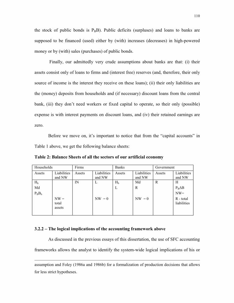
110

the stock of public bonds is PBB). Public deficits (surpluses) and loans to banks are

supposed to be financed (used) either by (with) increases (decreases) in high-powered

money or by (with) sales (purchases) of public bonds.

Finally, our admittedly very crude assumptions about banks are that: (i) their

assets consist only of loans to firms and (interest free) reserves (and, therefore, their only

source of income is the interest they receive on these loans); (ii) their only liabilities are

the (money) deposits from households and (if necessary) discount loans from the central

bank, (iii) they don’t need workers or fixed capital to operate, so their only (possible)

expense is with interest payments on discount loans, and (iv) their retained earnings are

zero.

Before we move on, it’s important to notice that from the “capital accounts” in

Table 1 above, we get the following balance sheets:

Table 2: Balance Sheets of all the sectors of our artificial economy

Households Firms Banks Government Assets Liabilities

and NW Assets Liabilities

and NW Assets Liabilities

and NW Assets Liabilities

and NW Hh Md PBBh

NW = total assets

IN L NW = 0

Hb L

Md R NW = 0

R

H PBΔB

NW= R - total liabilities

3.2.2 – The logical implications of the accounting framework above

As discussed in the previous essays of this dissertation, the use of SFC accounting

frameworks allows the analyst to identify the system-wide logical implications of his or

assumption and Foley (1986a and 1986b) for a formalization of production decisions that allows

for less strict hypotheses.

111

her assumptions about the structure of the economy. As the identification of these logical

implications is at times an arid task, some readers might want to skip this section, going

directly to the ones discussing behavioral hypotheses. It’s our understanding, however,

that the material in this section is crucial for the story we are trying to tell, so we must

encourage the reader to persevere at this point183.

First of all, from the firms’ column in Table 1 above we know that:

(AI.1) Y ≡ C + G + ΔIN ≡ FE + ΔIN [i.e, total expenditure and, therefore, total income is

identical to “final expenditure” (FE ≡ C + G) plus the accumulation of inventories by

firms (ΔIN)184].

Now note that, given that ours is a closed economy:

(AI.2) Y ≡ YG +YP [i.e, total income is identical to government plus private incomes].

This is true both before and after the “gross” incomes are altered by transfers and interest

payments (becoming then “net” or “disposable” incomes), though it will be more

convenient for us to use the second definition:

(AI.3) YG ≡ Government’s “net” income ≡ T + igR-1 - XB-1 ≡ Y- YP [i.e, government’s

“net” income is identical to total tax receipts plus the interest received by the government

minus the interest paid by the government – see Table 1 above].

Turning now our attention to the private sector (i.e., the aggregate of households,

firms and banks), we saw in the second essay of this dissertation (section 2.3.2) that, if

183 As put by G&C (1983, p.44), “we must exploit logic so far as we possibly can. Every purchase

implies a sale; every money flow comes from somewhere and goes somewhere; only certain

configurations of transactions are mutually compatible. The aim here is to show how logic can

help us to organize information in a way that enables us to learn as much from it as possible”. 184 Desired or not, as we will discuss in more detail in section 3.2.3 below. Note also that in our

accounting all goods and services are provided by firms in the non-bank business sector.

112

the net worth of both banks and firms is zero (or, equivalently, if all their after tax profits

are distributed), private disposable income equals households’ disposable income. But,

from (the households’ column of) Table 1 above, it’s clear that:

(AI.4) YP ≡ Private “disposable” income ≡ Y -YG ≡WB+ F+ XB-1 [i.e, private

disposable income is identical to wages plus after tax profits plus the interest received by

households, if the net worth of firms and banks are both zero].

Now note that, from (AI.1) and (AI.2), we have that

C + G + ΔIN ≡YG +YP

or, rearranging,

(AI.5) YP –(C + ΔIN) ≡G – YG ≡ -Sg

The identity above has a clear intuition. Given that total income is identical to total

expenditure (including expenditures in inventories), we have that if any sector spends

more than what it gets, it will be generating more income than what is getting and

therefore this “deficit” has to be compensated by a “surplus” in the other sector.

From the government’s uses and sources of funds in Table 1 above, we can also

write that:

(AI.6) ΔGD ≡ÛΔH + PBΔB ≡ G–YG+ΔR ≡ -Sg+ΔR [i.e, the increase/decrease in

government debt (ΔGD) is identical to the government current deficit (G–YG) plus the

(net) increase in government’s loans to banks]. If the bank’s stock of discount loans is

constant, the identity above simplifies to:

(AI.6a) ΔGD≡ÛΔH + PBΔB ≡ G – YG ≡- Sg

Indeed, as discussed in the second essay of the dissertation (section 2.2.3), in a model

with high-powered money the change in public debt doesn’t consist only of the G-YG

113

(-Sg, that can be called the “fiscal” component of public deficit) but also of (net) increases

in discount window loans (ΔR, that also changes the stock of high-powered money and,

therefore, public debt).

It so happens that the government is the source of great part of the private wealth

in this artificial economy. As we saw in section 2.3.2 above, the stock of net private

wealth is equal to the stock of net household wealth when the net worth of both banks

and firms are zero185. Therefore, from the households’ column in Table 1 above, we have

that:

(AI.7) PNW ≡ HNW ≡ FAt ≡ Hht + Mdt + PBBt

where the FA notation is meant to emphasize the fact that all wealth consists of financial

assets. In words, if the net worth of firms and banks are both zero, the total value of the

net private wealth of the economy is given by the stocks of cash and money deposits of

households (or simply the stock of money of households) plus the value of the

households’ stock of public bonds.

The last two relationships above seem to imply a direct link between public

deficits and private wealth. To see this, note first that from the households’ column in

Table 1 above we have that:

185 In more complex Godley-type models (in which M-M type assumptions are not used), it

becomes important to differentiate between the net worth of the private sector as a whole (i.e., the

sum of households’, firms’ and banks’ net worth), the net worth of the non-banking private sector

(i.e the sum of households’ and firms’ net worth) and the net worth of households.

114

(AI.8) YP – C ≡DWB + F + XB-1– C ≡ ∆FA186 [or, in words, what families get

(YP≡WB+F+XB-1) minus what they spend (C) is identical to what they save or dissave

(∆FA)].

Now note that, from the firms’ column in Table 1, above we have that:

(AI.9) ∆IN ≡ ∆L ≡ ∆PD [i.e., the change in the value of the inventories (valued at cost)

held by firms is identical to the change in the value of their bank loans and, given our

hypotheses, the change in the value of their total debt].

And, from (AI.8) and (AI.9) above, we can write:

(AI.10) YP –(C + ΔIN) ≡ÛΔFA - ΔPD [i.e, the private sector surplus (YP –(C + ΔIN)) is

identical to its net acquisition of financial assets (ΔFA) minus the net increase in firms’

debt (ΔPD)].

To get the precise relationship between the government’s deficits and the increase

in private wealth, one has to notice that, from (AI.5), (AI.6) and (AI.10), we have:

(AI.11) ΔFA ≡ ΔPD - Sg ≡ΔPD + ΔGD – ΔR [i.e, the change in households’ financial

assets (ΔFA) is identical to the change in the net debt of the firms (ΔPD) plus the

government’s current account deficit (-Sg) which, by its turn, is identical to the

increase/decrease in government debt (ΔGD) minus the (net) increase of government

loans to banks (ΔR)]. Again, in the absence of rediscount loans, we would have:

(AI.11a) ΔFA ≡ ΔPD + ΔGD

What this means in practice is that, in our artificial economy (and, for that matter, in all

closed economies), government deficits increase private wealth in a one-to-one basis.

Note also that, consolidating the balance sheets of households, firms and banks (i.e., the

186 Assuming that capital gains are zero (i.e., PB is constant).

115

private sector) in Table 2 above, it’s possible to get a “stock” version of the result above.

Indeed, by doing that one gets::

FA ≡ Hh +Md + PBBh + IN + Hb +L – L – Md – R (given that IN≡L and Hb+L ≡ Md +R).

Or, rearranging,

(AI.12) FA ≡ H + PBB + IN – R ≡ GD + PD –R (given that PD ≡ ΔIN and H+ PBB ≡GD)

This fact will play an important part in what follows.

3.2.3 - The behavior of the non-bank business sector

The story here is pretty much Keynesian. In the beginning of the production

period firms formulate expectations about the quantities they will be able to sell at given

“normal” prices and decide how much to produce (and how to finance production)

accordingly. As discussed in some detail both in the second essay of the dissertation and

in the previous section, the typical assumption in Godley-type models is that all

production (including inventory accumulation) is financed through bank loans and,

therefore, whenever they increase (decrease) their inventories, firms borrow (pay) from

(to) banks the exact amount required (available) to do so187. The accounting identity n.9

presented before formalizes this point:

187 See section 2.3.3 for a discussion. Note also that Circuitists, Post Keynesians and Marxists

share (a weaker version of) the same view. As put by Fontana (2000, p.33) “circuitists have

emphasized the distinction between firms, which are involved in income-expenditure decisions,

and banks, that is, suppliers of credit-money. For any production process, it is argued, firms need

to negotiate loans with banks”. Davidson (1972, p. 269-270), by its turn, points out that “if the

demand for capital goods [including working capital goods] is to increase, it will be necessary for

entrepreneurs to obtain additional command of resources. (…) but the obtaining of command of

resources requires the co-operation of the banking system and financial markets”. Finally, Foley

116

∆IN ≡ ∆L ≡∆PD (AI.9)

where ∆IN, ∆L and ∆PD are, respectively, the change in the value of the inventories

(valued at cost188) held by firms, the change in the value of their bank loans and the

change in the value of their total debt. Note also that this result is a direct consequence of

the hypothesis that retained earnings (and, as a consequence, the net worth of the firms)

are zero in this model and, therefore, “profits”189 can be seen as the capitalist’s family

income (since we are not assuming equity markets here)190.

Turning now our attention to the production decisions of firms, the hypothesis is

that they are based on firms’ expected sales “plus the change in inventories they want to

bring about” (Godley, 1996, p.14). In early (New) Cambridge-type SFC models the

(1986a, p.111) remarks that “the capitalist borrows in the first instance in order to use the money

received as money capital, to commit it to the circuit of capital (…)”. Foley and Davidson,

however, explicitly recognize that not all investment in production is necessarily financed by

loans. To use Hicks’s (1974, p.51) concept, Godley seems to work with a 100% “overdraft” non-

banking business sector, i.e., one that is “supported by assured (or apparently assured) borrowing

power” (the other extreme, according to Hicks, would be the “auto” sector, i.e., one “which

mainly relies for its liquidity on the actual possession of liquid assets”). 188Godley (see G&C, ch.9 or Anyadike-Danes et.al., 1987) prefers to consider the interest rate as

a part of the variable cost of firms. This apparent detail has the important implication that, for

Godley, increases in the interest rate would ceteris paribus increase prices as well. In our model,

on the other hand, increases in the interest rate ceteris paribus cause the dividends paid to owners

to fall. Ours seems the only way to go if one wants to discuss monetary policy issues and

simultaneously avoid inflation accounting complications. 189 As mentioned in the second essay of this dissertation, the definition of “profits” used here is a

loose one and means “what is left from what is sold after one pays for what it did cost”. Joan

Robinson (1956,p. 44) calls this concept “quasi-rent”. 190 Again, this assumption would have to be dropped in more sophisticated models since, as put

by Godley (1996, p. 8), “it is absurdly unrealistic, by-passing and trivializing the role of the

financial system (…)”.

117

assumption is that firms “correctly foresee” final sales and are always able to keep the

stock of inventories (valued at cost) as a fixed proportion of past final sales valued at

market prices [e.g, INt = γFEt-1= γ(C t-1+G t-1)]. This assumption makes the dynamics of

the model easier to analyze but is not one that is easy to justify. G&C (p.108, footnote)

try to do it arguing that “this might be the case, for example, if (…) [firms] have enough

foresight and flexibility to avoid a fall in inventories in a period when sales rise (…) and

if they manage to “catch-up” with a past change in the flow of sales by the end of the

period after the one in which the flow of sales changed”. Note however that, even in the

most favorable case for G&C’s argument, i.e., one in which the technology is flexible

enough to allow changes in production within the production period and/or if the

accounting period is much larger than the production period, it’s still difficult to explain

why firms would care to adjust their inventories to past sales if they can “sufficiently

foresee” (near) future ones.

Here we’ll proceed differently and assume that (i) firms’ expectations about

future final sales (FE= C+G) are adaptative (in the sense that in the beginning of the

production period t firms expect to sell in t+1 what they sold in t-1), (ii) the technology

doesn’t allow quantity adjustments within the production/accounting period and (iii) the

desired (but not necessarily the actual) stock of inventories in period t (valued at cost) is

proportional to expected final sales in period t+1(valued at cost)191. Formally,

191 In this sense our hypothesis is similar to the one in Hicks (1965, p.106) according to which

“desired working capital must clearly depend upon the expected level of output; it should thus

(…) depend upon Yt, Yt+1,...,Yt+n, where n is the number of periods that are taken by the

process of production (…) that takes the longest”. Note, however, that in our model n=1 by

hypothesis and therefore it seems natural to assume that the only expectation affecting firms’

desired working capital will be their expectations of final sales in period t+1.

118

E t(FE t+1) = FEt-1 (eq. 1)

and

INt* =gγE t(FE t+1)/(1+m) = γFEt-1/(1+m)192 (eq.2)

where INt* is the desired stock of inventories in the end of period t (valued at cost), γ is

the desired stock (of inventories, valued at cost)-flow(of sales, valued at cost) ratio of the

firms as a whole, FEt is the value (at market prices) of the total expenditures of the

economy in final goods in period t and m is the mark-up [so FEt/(1+m) = final sales

valued at cost].

Now note that, as we’re not assuming that firms have perfect foresight, we need to

say something about how firms deal with their falsified expectations. Here we’ll assume

an “extreme” version of the so-called “Stock Adjustment Principle” (see Hicks, 1965,

p.96), i.e., that in the beginning of each period firms adjust production to try to get their

desired stock of inventories. To make the content of this assumption clear let’s return to

the example given in the second essay of this dissertation (section 2.3.3), in which a firm

is in a steady state producing and selling 100 (valued at cost) at each period of production

(note that in this case γ = 1). Now let’s assume that, in a given production period t, the

firm unexpectedly sells 90 instead of 100. In this case inventories at the end of period t

will be 110 (100 produced + an involuntary increase in inventories of 10). Given our

story so far, in the beginning of t+1 the firm will expect to sell 90 in t+2 (i.e., what it sold

192 The hypothesis here is slightly different from the one in G&C(1983, ch.6). G&C assume that γ

is the desired stock(of inventories valued at cost)-flow (of sales valued at market prices) ratio,

while our γ is the desired stock(of inventories, valued at cost)-flow (of sales, valued at cost) ratio.

To put it another way, G&C’s γ is equal to our γ/(1+m). Contrarily to what happens in G&C (that

119

in period t – see eq.2) and its desired stock of inventories in the end of t+1 will be 90 =

1*90 (see eq.3). What our “extreme” version of the stock adjustment principle says is that

in such a case the firm will produce 70 in t+1 (i.e, expected sales of 90 – “excess

inventories” of 20). Formally, Xt (production in t valued at cost) is given by:

Xt = δ1Et(FE t+1) + δ1 [FEt-1 – Et-1(FEt)] + γ δ1 [Et(FE t+1) – Et-1(FEt)]

where, δ1 = 1/(1+ m).

or, given the assumption in equation (1),

Xt= δ1 [(2+γ)FEt-1 – (1+γ)FEt-2 ] (eq 3).

Note that the adjustment process assumed here is “extreme” in the sense that

firms try to get rid of all undesired inventories in a single period of production while

other more gradual kinds of adjustment are not only possible but (supposedly) more

common in practice193. Note also that in practice γ will be bigger than one so the firms

have a “cushion” to accommodate sudden increases in demand. Note, finally, that the

actual accumulation of stocks (valued at cost) is given by what is produced (Xt) minus

what is sold (valued at cost, i.e., FEt/(1+m)):

ΔIN = Xt – FEt/(1+m) = δ1 [(2+γ)FE t-1 - (1-γ) FE t-2 - FEt] (eq.4)

3.2.4 - The behavior of households

don’t discuss stock adjustment issues), however, our stock adjustment algebra requires an explicit

differentiation between market values and costs. 193 For nice discussions of possible adjustment mechanisms for the stock of inventories of firms,

see Hicks (1965, ch.10) and Blinder (1990, ch.5). The possibilities in this area are numerous.

120

We’ll work here with the classic Godley-type assumption that households as a

whole have a relatively constant desired stock(of wealth)-flow(of disposable income)

ratio. Formally, this hypothesis means that:

FA* = aαYP (equation 5),

where FA* is the households’ desired stock of wealth (that in this simplified model can

only be kept in either money, i.e., cash or bank deposits, or bonds), α is the stock flow

norm and YP is the flow of disposable income.

A second assumption here is that “the change in the stock of money [and bonds of

households] which actually takes place in any period is a certain proportion, Φ, of the gap

between the stock of money [and bonds] inherited from the previous period, FAt-1, and

the stock of money [and bonds] warranted by the current income flow, FA* (G&C, p.61).

This “partial adjustment mechanism” is essentially the same discussed in the second

essay of this dissertation and can be written formally as follows:

∆FAt = Φ(FA*– FAt-1) (equation 6)

In order to understand exactly what the assumption above means, let’s consider a

steady state in which the flow of disposable income is 10,000 per period, the stock-flow

norm is ¾ and the stock of financial assets (wealth) is 7,500. In this case, there will be no

change in FA from period to period (given that FA*= FAt-1). Now let’s assume that there

is a once and for all change in the flow of income per period to, say, 12,000 and that

Φ(the “speed of adjustment parameter”) is ½. In this case, we have that the “new” FA*=

¾*12,000 =9,000 >7,500 = FAt-1. This means that in the first period after the change in

income, ∆FAt = ½*(9,000 – 7,500) = 750, while in the second period ∆FAt = ½*(9,000–

8,250) = 375 and so on. Note that, by hypothesis, households can only buy (non durable)

121

final goods or accumulate financial assets and don’t have access to bank credit. This

means that ∆FAt is equal to the total savings of households and, therefore, in the example

above households as a whole will save 750 of their ∆YP in the first period, 375 in the

second period and so on. As Moudud (1998, p.97) puts it “Godley and Cripps propose a

theory of an endogenous saving rate which is based on the notion of a stable stock-flow

norm α” [and, I should add, a given process of stock (of wealth) adjustment]. Note, in

particular, that in equilibrium households spend all what they get.

As discussed in the second paper of this dissertation (section 2.3.2), the

hypotheses above imply a linear consumption function a la Modigliani (with lagged

wealth), i.e., of the kind C = c0YP + c1FAt-1.. A little bit of algebra will help us to get this

point clear. Note first that from (AI.8) above we have that:

YP – C ≡ WB + F + XB-1– C ≡ ∆FA (AI.8)

But from (5) and (6) above we have that:

∆FAt = Φ(αYP– FAt-1) (equation 7)

Now, replacing (7) in (AI.9) we have that:

YP – C= Φ(αYP– FAt-1)

and, therefore,

C = (1- Φα)YP + ΦFAt-1 (equation 8)

Here we’ll use a convenient special case of the equation above (often used also by

Godley, since it greatly simplifies the algebra) and assume that Φ=1/(1+α). G&C justify

this apparently arbitrary (though harmless simplifying) assumption as follows (p.92): “the

total amount of funds available for spending in any period (always assuming no

borrowings) is equal to the flow of income in that period plus the stock of money [and

122

bonds] inherited from the previous period (i.e, Y+FA-1) Let us now assume that in

deciding how much of the total funds available will be spent in any period, the income

flow Y, ranks one-for-one with the inherited stock of money FA-1. [For this to happen Φ

must be equal to 1/(1 + α)]”. Indeed, replacing Φ = 1/(1+α) in eq.8 above, we have that:

C =(YP + FAt-1) /(1+α) (equation 9)

and, therefore, households spend the same proportion of their current and previously

unspent past incomes. This is precisely what G&C mean when they say that “Y ranks

one-to-one with the inherited stock of money” [and bonds] in the households’

expenditure decisions. The (algebraic) convenience of this assumption is that (it’s easy to

prove that) it implies that:

C = FA/α194 (equation10).

Our final hypotheses concern the portfolio choice of households. As in the IS/LM

model, we’ll assume that households have to choose between holding money (i.e, cash

and deposits, for simplicity we’ll assume here that the public only holds a small fraction,

say 10%, of money in cash) and bonds based on their liquidity requirements “to carry out

transactions” and on the assets’ real rates of return195. Formally we have:

Bhd = households’s bond demand = β(ib, Ct)* FAt (eq.11)

and

194 Indeed, if Φ=1/(1+α) then eq.8 above turns into ∆FAt = (αYP– FAt-1) /(1+α). As ∆FAt ≡ FAt -

FAt-1, simple manipulations lead us to the conclusion that FAt = α(YP + FAt-1) /(1+α) = α*C

(from equation 9). It’s interesting to notice, for historical reasons, that in early “New Cambridge”

models (in which, as discussed in the second essay of this dissertation, the stock-flow norm

applied for the private sector as a whole), this assumption would implied that FAt = α(C + I). 195 Which, given our hypothesis that prices are fixed, are ib = X /PB (for bonds) and zero (for

money).

123

Mhd = households’ money demand = µ( ib, Ct)* FAt 196 (eq.12)

where, ib = X /PB = interest on bonds and

β + µ = 1 (eq.13).

3.2.5 – The Behavior of Banks

As mentioned before, our treatment of the Banking Sector is admittedly an

extremely crude one. The main hypotheses here are that (i) banks “passively provide

loans to firms on the security of inventories” (Godley, 1999a, p.137)197, (ii) banks are

price takers, in the sense that the interest rate of their loans is exogenous to them and (iii)

banks’ retained earnings are zero. In other words, in the beginning of the production

period banks forced to give loans to (i.e, increase the deposits of) whichever firm asks, at

a fixed interest rate and in the end of the production period banks pay their owners (or get

from them) whatever profits (losses) they have. These are, of course, heroic hypotheses

and we used them here just to keep the algebra under control198. Less controversial are

the hypotheses that (i) the central bank forces the banks to keep a fixed proportion (ρ) of

their deposits as minimum reserves and (ii) any liquidity problems experienced by banks

are assumed to be solved by inter-bank loans (which don’t appear in the aggregated

196 Note however that, as Godley (1999a, p.397) reminds us “the term ‘demand’ for money strains

language, for it badly describes a situation where people aim to keep their holdings of money

within some normal range but where the sums they end up with are determined in large part by

impulse purchases, windfalls and unexpected events”. 197Kalecki’s “principle of increasing risk” is probably among the first of a series of models of

banking behavior in which loans are much harder to get than assumed here. 198 As discussed in the second essay of the dissertation, Godley’s own models assume that banks

are price makers.

124

accounts above) and/or discount window loans199. Last, but not least, we consciously

avoided all matters related to banks’ portfolio choice assuming that banks’ only assets are

loans to the “non-bank business sector” and reserves and that banks’ liabilities consist

only of households’ deposits and discount window loans.

It’s probably important to emphasize here that, under the hypotheses above (and

the ones previously made in section 3.2.1), banks have no degrees of freedom

whatsoever. In particular, banks have no control over whether they will be forced or not

to get discount window loans to fulfill their reserve requirements while simultaneously

providing cash to the public as demanded. Indeed, the volume of discount window loans

depends entirely on the initial size of banks’ reserves and the behavior of money demand.

It may, of course, be zero if, for example, there is a decrease in the demand for bonds and

people start to sell bonds back to government in a sufficiently large scale. Note, in

particular, that as the volume of loans and deposits are exogenous to banks (a hypothesis

kept by Godley in his most recent papers – see Godley, 1996 or 1999a) and they can’t

buy government bonds (by our assumption), reserves can be higher than the minimum.

As their loans to firms (and their related interest charges) are (sometimes only partially)

paid back along the production period, banks would then be able to decrease their debt

with the central bank (if necessary). Note, however, that as long as just a small fraction of

households’ money is held in cash and the interest rate on discount window loans is not

very high relative to the interest rate on their loans, banks will always be able to pay

positive dividends to their owners.

The assumptions above can be formalized as follows:

199The hypotheses here differ from the ones in G&C chapter 8, which describes a model without

125

Ls = Ld (eq.14)

Mds = Mdd (eq.15)

Hb = Bank Reserves = max {ρMdt , Mdt – Lt} (eq.16)

R = Discount Loans = - min {0, Hb - ρMdt} (eq.17)

3.2.6 - The Behavior of the Government

The important assumptions here are three. First, government is assumed to choose

the amount of its expenditures with goods and services (G) and to tax people in such a

way that YG (government’s net income, i.e, taxes minus interest payments on public debt

plus interest on discount window loans received) is a fixed proportion of the national

income. Formally, YG =θY, where θ is also a policy variable (see G&C, p.107). In sum,

the government can choose G/θ, the “fiscal stance” of the economy. Second, the central

bank is assumed to set the compulsory reserves of banks and to act as a lender of last

resort through the so-called “discount window” loans to banks (with interest rates fixed

by the central bank itself) whenever necessary. Third, monetary policy is assumed to be

“permissive, in the sense that the central bank holds the interest rate [on public debt]

constant” (Solow, 1983, p.165)200. Therefore, in the present model “cash is provided on

demand to the public. The government, or the central bank, does not decide in advance on

high-powered money. They are used in Godley (1996 and 1999a), though. 200 A post-keynesian endogenous money view would probably disagree with Solow’s choice of

words. The control of the interest rate is seen by this school as a pragmatic and sensible decision

of the central bank, given the (Minsky-type) risks of attempting to control the “money supply”

“(…)by adjusting [central bank’s] holds of bills (thus changing the level of non-borrowed

reserves of commercial banks) or by altering reserve requirements(…)”(Taylor, 1997, ch.7, p.11).

126

the proportion of the deficit that will be “monetized”. This proportion is set by the

portfolio decisions of the households, at the rate of interest set from the onset by the

monetary authorities”(Lavoie, 2001, p.5).

The assumptions above can be formalized as follows:

ib = X/PB = ib* (eq.18)

Bs= Bd( ib*) = β( ib*, Ct)*FAt (eq.19)

G = G0 (eq.20)

YG = θY (eq.21)

and, given that Y ≡ YG +YP (AI.2),

YP = Y - YG = (1- θ)Y (eq.22)

3.3 – The “Within Period” and “Between Periods” Properties of the Model

After having presented the structure of the model in detail it is now time to

discuss its formal solution and its dynamic properties. We do that in 4 steps. First we find

the “one period” algebraic solution of the model (in section 3.3.1) and discuss theoretical

issues related to it (in section 3.3.2). Then we formalize and discuss both the steady-state

(in section 3.3.3) and the dynamics of the model “between periods” (in section 3.3.4).

Mathematical proofs related to the necessary and sufficient conditions for the dynamic

stability of the model can be found in the appendixes.

As mentioned in the section 1.2.2 above, almost all central banks of the world are now

127

3.3.1 - The “One Period” Solution of the Model

From (AI.1) and (eq.4) above, we have that:

Yt = FEt + δ1 [FEt-1 + (FEt-1 – FEt-2) + γ(FE t-1 – FEt-2) – FEt]

where, δ1 = 1/(1+ m).

And given that FEt ≡ Ct+Gt and Gt=Go, one can rearrange the expression above to get:

Yt = δ1 [m* Ct + mGo + (2+γ)FEt-1 - (1+γ)FEt-2]

Now, all we need to do is to replace (eq.9) and (eq.22) in the equation above and

solve for Yt to get:

Yt = a1*FA t-1+ a2*Go+ a3*FEt-1 + a4*FEt-2 (eq.23)

where,

a1 =m*[(1+m)(1+ α) – m(1- θ)]-1

a2 =(1+ α) m*[(1+m)(1+ α) – m(1- θ)]-1

a3 = (1+ α)(2+γ)*[(1+m)(1+ α) – m(1- θ)]-1

a4 = - (1+ α)(1+γ)*[(1+m)(1+ α) – m(1- θ)]-1

And, as we can see, Yt is function of 5 exogenous variables of the model (γ, Go, α, m and

θ) and the predetermined values of FEt-1, FEt-2 and FAt-1. It is also clear that, given the

value of Yt, we can easily determine the values of the other endogenous variables of the

model201.

“permissive” in Solow’s sense. 201 Indeed, given Yt and the values of the predetermined and exogenous variables, the values of

YG, YP and C are immediately determined by equations (21), (22) and (9). But given the values

of YG, YP and C, one can determine also ΔIN (with AI.1and eq.20), ΔL and ΔPD (with AI.9), -Sg

(with AI.5), and ΔFA (with AI.11). The remaining of the solution is trivial if one notes that the

households’ assets demands are fully determined (by equations 11-13), if YP and ΔFA are

known.

128

3.3.2 – Is there a story for what happens “within the period”?

The algebraic solution presented above implies a couple of theoretical issues that

deserve some discussion. First, equation 23 above doesn’t describe an equilibrium in any

sense of the term. In fact, if all behavioral assumptions hold true, it gives us the precise

ex-post values of total income and expenditure (as defined above) even if firms’ ex-ante

expectations are completely falsified in practice. As discussed in the second essay of this

dissertation (sections 2.2.6 and 2.3.5), this “disequilibrium” view underlying the model is

essentially the same espoused by Yale-type SFC theorists. It doesn’t mean, of course, that

one cannot come up with a theoretical “single period” equilibrium for the model202, but

that such a concept is useful mostly to the specification of the dynamics of the model

“between periods”. We’ll return to these issues in sections 3.3.3.and 3.3.4 below.

Second, in the model above financial variables are entirely determined by:

(i)saving and portfolio decisions of households, and, especially, (ii)production decisions

of firms and (iii) the fiscal stance and the interest rate fixed by the government. In other

words, there is no “feedback” whatsoever from the “monetary side” over the “real side”

in this model, for the very good reason that the interest rate is given by hypothesis203.

202 That would require – as discussed in sections 2.2.5 and 2.2.6 above - the modeling of ex-ante

expectations of households and banks as well. Note, however, that as banks are completely

passive in this model, their expectations won’t make any difference to the results. 203 Pretty much like in the “New Consensus” literature (see section 1.2.2 above). It’s interesting to

notice that, at least in this particular sense, mainstream economists have converged to a view long

espoused by Godley, Kaldor and other Cambridge economists. Note, however, that their

interpretation of this hypothesis is completely different. Neoclassical Keynesians (“Old” and

“New”, as well as some Post Keynesians) would probably interpret it as a “horizontal LM curve”,

while the concept of a “LM curve” (which portrays an alleged “equilibrium” between a stock and

a flow), horizontal or not, is alien to Godley-type models.

129

Third, it’s our contention that the general “view” (in Schumpeter’s sense) of the

economy underlying Godley-type models is perfectly compatible with the broad

Circuitist, Post Keynesian and Marxist views on macroeconomic dynamics204. Authors

from all these traditions would probably agree with Keynes (1930, vol.1. p.282) that

“credit cycles” are somewhat akin to chess matches, in the particular sense that “one can

describe the rules of chess and the nature of the game, work out the leading openings and

play through a few characteristic end games; but one cannot catalogue all the games

which can be played”. The remaining of this section will focus precisely on the “leading

openings” and “characteristic end games” assumed both in Godley-type models and in a

few similar Circuitist, Post Keynesian and Marxist ones.

Beginning with the “openings”, it’s interesting to notice that the “within the

period” story in Godley-type models starts pretty much like, for example, Graziani’s

(1996, p.143): “Let us imagine a pure credit economy, in which all payments are made by

bank checks. Let us consider only consolidated macro sectors: banks, firms, and wage

earners. Banks grant loans to firms, the outlays of which are exhausted by the wage bill.

The moment wages are paid, firms become the debtors of the banks and wage earners the

creditors of the same banks. A triangular debt-credit situation, typical of any monetary

economy, is thus created. A picture of the economy taken immediately after the payment

of wages would review that the whole of the existing money stock is a debt of the firms

and a credit of wage earners towards the banks”. As mentioned before, the Post

Keynesian and Marxist “openings” are essentially the same, with the qualification that

they stress also the role of other sources of finance/funding of firms, notably retained

204 Even if one accounts for the flagrant heterogeneity of the authors in these schools of thought.

130

earnings205. But few authors in these traditions would deny that in modern capitalist

economies bank credit responds for a large amount of the investment in working capital

and, therefore, the pertinence of the theoretical exercise proposed here.

So far so good, but what about “next”? Again, the story implicit in Godley-type

models206 doesn’t seem particularly controversial. It is, for example, similar to

Davidson’s (1972, p. 271), according to whom households will respond to this “increase

in (…) [their] money balances” by making “consumption expenditures and consequently

hold[ing] some of the additional money for transaction purposes. The remainder becomes

households savings [Sh] and the households must decide in what form to store wealth”207.

And, then again, essentially the same point is corroborated by both Graziani (1996,

p.143) and Foley (1986a, ch.5). In fact, as far as households’ behavior is concerned, the

only major difference between Godley-type models and the conventional Post-

Keynesian/Circuitist/Marxist stories has to do with the implications of the “stock-flow

norm” for the precise specification of the consumption function.

After this point, as much as in a chess game, it’s impossible to tell what will

happen in practice. Surely, a very complex web of transactions both between and within

205 As much, by the way, as Godley himself. See, for example, Godley (1996, p.8) or Lavoie and

Godley (2001-2002, p.111). The simplifying hypothesis used above is aimed only to emphasize

the importance of bank credit in Godley’s story. 206 See, for example, G&C, chapter 3. 207 Davidson’s story is, however, significantly different from Godley’s, among other things

because it includes also investment in fixed capital and complications related to transactions

between firms (that are simplified away here). Moreover, despite all the complexities implied by

his (literary) dynamic narrative, Davidson appears to be comfortable with the conventional

Keynesian idea that the economy does arrive to a static “short period equilibrium”.

131

the macroeconomic sectors will take place208, but Godley-type authors (and, for that

matter, all the other schools of thought discussed here) have nothing to say about the

precise timing of these transactions in historical time. As far as we know, the best attempt

to do it in this broad literature is due to Foley (1986a, ch.5 and 1986b, p.20-30), who

explicitly models the “lags” of the various decisions of both households and firms,

although leaving the determinants of these lags open209.

Turning now our attention to “characteristic endings”, it’s interesting to note that

the story implicit in Godley-type models is again pretty much like the one told by

Graziani (1996, p.143): “As soon as wage earners spend their incomes, money flows back

to the firms. (…) If no hoarding takes place, the proceeds originating from sales of

commodities (…) enable firms to repay the whole of their debt to the banks. It need not

be added that firms, besides giving back the principal of their loans are held to pay

interest on them”. Four qualifications must be made here, though.

First, it’s important to keep in mind that, as originally pointed out by Marx210 and

summarized here by Kaldor (1996, p.33, emphasis in the original): “even if we abstract

from compulsory levies on income imposed by the government etc, and if we suppose

that wage earners spend the whole of their wage income on purchasing goods in the same

period, without saving anything for a rainy day or for retirement, their total outlay of

goods cannot be greater than the total costs of these goods incurred by the entrepreneurs,

leaving nothing over for profit, the expectation of which was the entrepreneur’s sole

motive in producing goods for sale. To make it possible for the entrepreneurs as a class to

208 A very nice description can be found in the introduction of Backus et. al. (1980). 209 Foley’s reasoning builds on his critique of “period models” presented in section 1.2.3 above. 210 In his discussions of the Circuit of Capital (see Foley,1986, ch.5).

132

realize profit over and above the costs incurred, there must be an additional source of

demand which is autonomous (or exogenous) in character, which does not flow directly

from income receipts generated by current production, and thus will determine at what

level of output total demand and supply will match one another”. Second, even if we add

“autonomous expenditures” (i.e., ones that don’t depend on the income generated by

current production) to the story, it’s by no means certain that firms will be able to repay

their debts to banks. Hoarding does happen in practice and sometimes firms just can’t sell

what they produced. Third, even if firms’ expectations are not falsified, their ability to

pay their loans depends in important ways on what happens with their stock of

inventories and the way these inventories are financed211.

All three qualifications made above are non-controversial in nature and this leads

us to the fourth. It’s our contention that what truly separates Godley-type models from

the conventional Post-Keynesian and Circuitist ones mentioned above is that the former

emphasize that the story cannot end up in “one period” or, for that matter, in the “short

run”212. Indeed, up until now the story doesn’t differ much from more conventional

Keynesian ones, albeit stressing the importance of bank credit for the financing of firms

and of wealth for the consumption of households and being less respectful as far as “the

Keynesian short period equilibrium” is concerned. Note, however, that Godley-type

models (as much as Marxist ones, for that matter) are essentially dynamic in the sense

that they emphasize and aim to “capture“ (hence their emphasis on accounting) the

211 If, for example, firms end up the “period” with a positive stock of inventories and these are

financed with loans, it’ not obvious that they will be able to pay “the whole of their debt” to

banks.

133

precise dynamic implications of the stock–flow relations between macroeconomic

variables - notably between the stocks of assets and debts of the macroeconomic sectors

and their (interconnected213) flows of income, expenditures, savings and net

borrowing/lending214. These “dynamic implications” are precisely the topic of sections

3.3.3 and 3.3.4 below.

3.3.3 - The Steady-State of the Model

As usual in this kind of analysis, Godley-type dynamic stories start “with the

consideration of a steady-state (….) [and] then consider the implications of well defined

shocks to exogenous variables and see how the system reacts. Although the exposition is

concerned with steady-states and shocks it will be apparent that the analysis can be

readily adapted to deduce how the system should behave in more complex, realistic

contexts, where the exogenous variables behave in a thoroughly disorderly way” (G&C,

p.48). In the present section we will discuss the steady-state of the model. The next

section considers the ‘implications of well defined shocks to exogenous variables’.

212 In this particular sense, Godley’s point is exactly the same made by Christ (1967 and 1968),

Blinder and Solow (1973) and Tobin and Buiter (1976, 1980) 213 Again the accounting plays a crucial role, making these interconnections explicit to the

analyst. 214 The main dynamic mechanism underlying Marxist models is, of course, the capitalist need to

accumulate (and, therefore, reinvest). As a consequence, Marxist models tend to emphasize

“supply-side” stock-flow relations (like, for example, those between the stocks of capital and the

reserve army of labor and the flows of income, investment and profitability). It seems possible to

make a case for the complementarity between Godley-type models (or, for that matter, “demand-

side” SFC models in general) and Marxist “supply-side” dynamic models, though this is beyond

the scope of the present paper.

134

Here we will follow G&C (p.110) and define the steady state of the model as a

situation in which all the stock variables of the model are constant and (p.160) “(…) the

non-bank business sector (…) regard(s) the composition of (…) [its] portfolio of assets as

appropriate or sensible given banks’ interest rates and bond yields”215. Putting it another

way, the steady-state of the model is a situation in which ∆PD = ∆IN = Sg = ∆GD = ∆FA

=∆FE = ∆C = ∆R = ∆Md = ∆Hb = ∆Hp = ∆B = 0. To find it, one has first to notice that

from (AI.6a) we have that:

(AI.6a) ∆GD ≡ G – YG ≡- Sg

and, replacing equations (20) and (21) in the expression above:

∆GD = Go–θY

But in the steady-state, by definition, we have also that ∆GD = 0 and, therefore

Go – θY = 0

and, as a result,

Y= Go/θq(equation 24).

Of course, given the value of Y one can easily calculate the other endogenous variables

following the procedures of the previous section.

There are several important issues raised by this result. First, although it depends

entirely on the particular (stationary) notion of the steady-state adopted here, it can be

easily extended to (flow) steady-growth notions as well216. Second, it is important to

215 As a matter of fact, G&C include the requirement that also banks must consider their

portfolios of assets sensible. In our model, however, banks have no way to choose their portfolios

and have to be satisfied with whatever they get (see section 3.2.5 above). 216 Indeed, in a (flow) steady-growth state both Y and G grow at the same rate (say, “g”) and,

therefore, -Sg =G–θY (government current deficit) also grows at this rate, so that -Sg/Y is constant

(equal, say, to “k”). It’s, then, clear that in a (flow) steady-growth we have Yt = Gt/(k+θ).

135

notice that, despite acknowledging that in reality “exogenous variables behave in a

thoroughly disorderly way” (and, implicitly, the heroic assumptions made in their

simplified theoretical model) G&C appear to think that the steady-state above (or, in

more realistic models, its steady-growth counterpart) is a true centre of gravity for real

world economies. Indeed, they state this view quite explicitly in the following passage:

“The (steady-state equilibrium income) is not just a hypothetical ‘equilibrium’ state in the

sense of being some timeless intersection of two curves. It is a prediction of the flow of

national income, which will actually become established in historical time if the

government adopts a particular fiscal stance and does not thereafter change it. This level

of income will be maintained continuously by flows between the government and the

private sector (..)” (p. 111)

Third, the following discussion establishes a certain hierarchy in the exogenous

variables. It is pretty clear that an once and for all change in the “fiscal stance” (Go/θ)

will change the long run centre of gravity of the economy, while a change in the other

exogenous variables of the model won’t and, therefore, will have just temporary effects.

One interesting result that stresses the importance of the fiscal stance in the long run

dynamics of the economy can be derived from equation (23) when FEt-2 = FEt-1 = FEt =

Y, Go = θY and FA-1 = FA. In this case, we have:

Appendix 2 discusses the necessary and sufficient conditions for the stability of this (flow)

steady-growth “equilibrium”. It’s important to notice that, beginning from an arbitrary

disequilibrium point, flow steady-growth only implies a stock-flow steady growth assintotically

(because the rates of growth of stocks depend also on their initial values) and, therefore, the two

notions are not the same. Recent applied work by Godley (see, for example, Godley, 1999c)

emphasizes yet a third related issue. i.e., the study of growth paths that do not imply explosive

growth of crucial stock-flow ratios.

136

Y = a1FA+ a2 θY + a3Y + a4Y

or, after some algebraic exercises,

Y = a1FA*[1 - a2 θ - a3 - a4]-1 = FA / α (1 - θ) (equation 25)

However, from (AI.12) we also have that:

FA ≡GD –R + PD

and, therefore, equation 25 above can be rewritten as follows:

Y = (GD - R + PD) / α (1 - θ) = steady-state income = Go/ θ (equation 26)

According to G&C(p.114), this equality “may seem a little surprising at this stage since it

has the powerful implication that fiscal stance (Go/θ) will somehow ultimately generate

the same aggregate income flow irrespective of the amount of private debt creation (PD)

and also independent of the money income norm (α). So it must be implying that more or

less private debt, so long as the fiscal stance is given, must give rise to a change of equal

and opposite size in the total government debt. We shall shortly be showing exactly the

mechanics of this displacement (our version of “crowding out”)”

The dynamics of the system (or, “the mechanics of this displacement”) is

precisely the topic of the next section of these notes.

3.3.4 – The story “between periods”: A formal treatment

Here it is assumed that the economy is initially in a (stationary) steady state and,

all of a sudden (in the first period of the analysis, it is hit by shocks in the exogenous

variables. As it will become clear in what follows, the story below can be readily adapted

to more complex settings217. Note that as the “monetary side” of the model is entirely

217 See, for example, the story in appendix2 below.

137

determined by the “real side” (see section 3.3.2 above), we will limit ourselves here to the

analysis of the dynamics of the latter.

A - The first “period”

Given that the “underlying economic stories” will depend on which exogenous

variable is shocked, it seems appropriate to start with the algebra (that doesn’t change as

much). We then illustrate the general algebraic exercise with the story of what happens

when the government increases its expenditures (Go).

We begin by noticing that from equation (23) above we can write:

dY ≈@∂Y/∂γ*dγ + ∂Y/∂m*dm + ∂Y/∂G0*dG0 + ∂Y/∂α *dα + ∂Y/∂θ*dθ +

∂Y/∂FE-1*dFE-1 + ∂Y/∂FE-2* dFE-2 + ∂Y/∂FA-1*dFA-1 (expression 1218)

And, therefore, the instantaneous impact on steady-state income of a change in any

exogenous variable X (i.e., γ, m, G0, α and θ) can be approximated by:

dY1 ≈ ∂Y/∂X*dX1 (expression 2)

Of course, income is not the only endogenous variable that instantaneously responds

to a change in the exogenous variables. In particular, both the consumption of the private

sector and private wealth (i.e., the stock of financial assets of households) are

immediately affected as well. As we saw before:

FE ≡ C + G (from AI.1)

C = [(1- θ)Y + FAt-1] / (1+ α)] (from equations 9 and 22)

C = FA/ α (eq. 10)

and therefore,

138

dC1 ≈ ∂C/∂Y*dY1 + ∂C/∂X*dX1 + ∂C/∂FA-1*dFA-1 (expression 3)

or, given that dFA-1 = 0,

dC1 ≈ ∂C/∂Y*dY1 + ∂C/∂X*dX1 (expression 4)

dFE1 = ∂FE/∂C*dC1 + ∂FE/∂G*dG1 = dC1 + dG1 (equation 27)

dFA1 = α dC1 (equation 28).

These results are important because, in the absence of further shocks, they will be

responsible for the whole change in total income in the next period.

The algebra above – based mostly on ex-post considerations and algebraic tricks -

doesn’t reflect clearly what supposedly happens “in practice” “within the period”.

Consider, for example, the case in which government expenditures are increased. The

first and obvious thing to notice in this case is that more things will be sold (throughout

the period) and, therefore, more income (i.e., profits, since wages and interest payments

are pre-determined in the beginning of the period) will be generated. As capitalists are

also households in this model (and, therefore, also have stock-flow norms to follow), part

of these extra profits will also be spent (again within the period), in such a way that C

will increase as well. The total impact on income and consumption can be approximated

by expressions (2) and (4) above (substituting X for Go). It’s not difficult to notice also

that the final impact in government’s current account deficit (-Sg) can be approximated

by:

d(- Sg)= dGo - θdY1≈ dGo - θ∂Y/∂G0*dG0 = dGo(1 – θ a2)219 (expression 5)

218 If Yt depends on X linearly then the expression holds as equality. If not, the quality of this

(linear) approximation will be negatively related with the size of the shock in X. 219 We know from equation (23) that ∂Y/∂G0 = a2

139

And, as usual, the “size” of the impact will depend on the parameters of the model but its

“sign” will be positive in all relevant cases.

As noted before, up until now the story is pretty much like the conventional

Keynesian with an “horizontal LM”. Notice, however, that while the latter ends at this

point, even a simplified Godley-type story is much longer. A first difference is that, by

hypothesis, firms’ expectations were falsified and, therefore, their stock of inventories in

the end of the period is below “normal”. But this also means that they will be able to

repay more of their debts to banks (since, from AI.10, ∆L≡∆PD≡∆IN) “within the

period”, what by its turn (together with government’s current deficit) will affect the net

stock of financial assets of the private sector (since, from AI.12, ∆FA≡ ∆PD-∆Sg).

Indeed, a second difference of Godley-type models is that all these changes in the

(interconnected) debts and assets of the various sectors are explicitly quantified and their

dynamic consequences analyzed (admittedly with “crude” hypotheses, but still). Clearly,

for example:

∆IN≡ -dFE1/(1+m)220= [∂FE/∂C*dC1+∂FE/∂G*dG1]/(1+m) =[dC1+dG1]/(1+m) (eq.29)

And, even though equation 28 above makes clear that the total impact on wealth (FA)

will be positive221, we could have derived this result without its help, just by inspection of

(AI.9), (AI.11), (expression5) and (equation 29).

220Note that while final expenditures are measured in market prices, inventories are valued at cost.

Hence the need to divide dFE by (1+m) 221 Equation (28) was derived from equation (10) which, by its turn, depends on the simplifying

hypothesis that Φ = 1/(1+ α) adopted in section 3.2.4 above.

140

B - The second “period”

Again beginning with generic algebra, we note that in the absence of further

shocks in the exogenous variables (i.e, under the assumption that dγ2 = dm2 = dG02 =

dα2 = dθ2 = 0) expression (1) above reduces to:

dY2 = ∂Y/∂FEt-1*dFEt-1+ ∂Y/∂FEt-2*dFEt-2 + ∂Y/∂FA-1*dFA1 (equation 30) 222.

Now note that dFEt-1 and dFAt-1 are both larger than zero (since in the previous period

there were changes in the final expenditure and in the financial assets of the economy),

but dFEt-2 is still zero (since in the period before the previous one the economy was still

in the steady state). We have, then, the following expression for dY2:

dY2 = ∂Y/∂FEt-1*dFE1 + ∂Y/∂FAt-1*dFA1 (equation 31)

and it is also true that

dC2 = ∂C/∂Y*dY2 + ∂C/∂FA-1*dFA1 (equation 32)

dFE2 = ∂FE/∂C*dC2 + ∂FE/∂G*dG2

or, given that dG2 = 0,

dFE2 = dC2 (equation 33)

dFA2 = α dC2 = α dFE2 (equation 34).

The story underlying the algebra above is apparently simple. Indeed, it’s easy to

notice that the main mechanisms in effect are: (i) the increase in consumption due to the

“partial” adjustment process assumed for households (which on one hand are now richer

and on the other have a new wealth target223) and (ii) the increase in production and,

222 Note that now we have an equation because Yt is a linear function of FEt-1, FEt-2 and FAt-1. 223 Since their disposable income has now changed. Note that the story here wouldn’t change

much if we were to add to this income/wealth adjustment process an additional component due to

141

therefore, income and wealth due to the “extreme” adjustment process assumed for firms.

The precise outcomes of these mechanisms are not generally clear, though, being heavily

dependent both on the parameters and on the precise adjustment processes assumed. In

the monotonic case generally assumed by Godley-type authors224, we would have a

further increase in income, in inventories and in the financial assets of households,

despite the reduction in government debt (due to the increase in net tax revenues).

C - The third “period” and after

In the monotonic case the story here is the same as above, while in the non-

monotonic case things get too dependent on the specific values of the parameters. The

algebra is straightforward, though. In the absence of shocks in the exogenous variables,

the increase in income in the third period is:

dY3 = ∂Y/∂FE-1 *dFE2+ ∂Y/∂FE-2*dFE1 + ∂Y/∂FA-1*dFA2 (equation 35).

The difference with respect to the second period is that now dFE-2≠0 (since in both the

first and the second periods there were changes in the total expenditures in final goods).

Also, as before,

dC3 = ∂C/∂Y*dY3 + ∂C/∂FA-1*dFA2 (equation 36)

dFE3 = dC3 (equation 37)

dFA3 = α dC3 = α dFE3 (equation 38).

households’ expectational errors (that in this case would look like the “generalized partial

mechanisms” discussed in section 2.2.6 above). That’s a possible rationale for the little

importance given to “single period” equilibrium concepts in earlier Cambridge models. 224 As discussed in section 2.3.7 above.

142

It should also be clear that the process will continue until infinite and that after the

third period, the dynamics of the model can be summarized by the following system of

difference equations:

dYt = ∂Y/∂FEt-1*dFEt-1 + ∂Y/∂FEt-2*dFEt-2 + ∂Y/∂FAt-1*dFAt-1 (equation 39).

dFEt = ∂C/∂Y*dYt + ∂C/∂FAt-1*dFAt-1 (equation 40)

dFAt = α dFEt (equation 41).

As mentioned before, Godley-type authors generally assume that the dynamic process

described by their models will be monotonically stable in all empirically relevant cases.

Whether or not this is true in the particular model presented here is not very clear, as

discussed in more detail in the appendix.

D– A General Point

A strong conclusion of stable versions of the model above (and, indeed, of any

model with a stable stationary stock-flow steady state225) is that deficits or surpluses are

necessarily temporary. No matter how big is the government deficit/private surplus (or

vice versa226), one knows for sure that the economy is converging to a steady-state in

which all stocks (including stocks of debt) are constant by definition and, therefore, no

deficits or surpluses can exist.

Although this conclusion depends entirely on the particular (stationary) version of

the steady-state used in Godley-type models, it’s interesting to notice that it does have a

225 Like, for example, the one presented in Blinder and Solow (1973). 226 As seen in AI.5, the private surplus is always identical to the government deficit. Note that the

private sector has necessarily to go into deficit in this model if the steady-state disposable income

falls (to enable its adjustment to a lower equilibrium stock of wealth).

143

more general (flow) steady-growth counterpart - widely used in Godley-type empirical

analyses227. Indeed, given that a stable (flow) steady-growth path implies that private

deficit/ public surplus (or vice-versa) are both constant relative to total income228, no

situation that involves a continuous increase of these variables (relative to income) is

sustainable229. In particular, no matter how rapid is the change in the private deficit

relative to GDP, one knows for sure that it won’t last. Note also that no sustainable

growth is possible with zero government deficits (for that would prevent the increase in

the desired private wealth caused by the increase in private disposable income)230.

3.4 - A Brief Note on the General Structure and Possible Extensions of Godley-Type

Models

The discussion above allows us to arrive to some general conclusions about

simple Godley-type models. We begin by reminding the reader of some very simple – but

often forgotten – points about these models and then proceed to discuss some important

details in their formal structure. All the conclusions below lead to some natural (and

possible) extension of the model presented above, making clear that a lot remains to be

done in this line of research.

227 See, for example, Godley, 1999c. 228 Appendix 2 provides a formal treatment of these issues. 229 Things get slightly more complicated in models of open economies, but the general message

remains essentially the same. 230 The same point is made, for example, by Tobin and Buiter (1980, p.106), according to whom,

“the balance of government budget is not a requirement of long run equilibrium (…). A constant

real steady-state deficit per unit of output provides for the required growth in the in the nominal

stocks of money and government bonds”.

144

The simple points we want to mention are two. First, simple Godley-type models

are “pure” demand models, in the sense that they assume away all kinds of constraints

coming from supply factors231. To put it briefly, if government expenditure is quadrupled

and the parameters are such that the model is monotonically stable, total income will

converge pretty quickly to its new (four times bigger) steady-state value232. Second,

Godley-type models are “period models” in the sense of Foley (1975, p.310), i.e., they

assume that ”all transactions of a certain class occur in the same, synchronized

rhythm”233. In the “real” world, firms don’t make production decisions all at the same

time, and to assume this is clearly (and admittedly234) a heroic hypothesis.

Turning now our attention to the details on the structure of the model, the points

we want to make here are five. First, it should be clear by now that the precise dynamic

behavior of the model is entirely dependent on the particular specification of the

adjustment mechanisms assumed for households’ stock of wealth/ flow of disposable

income and firms’ stock of inventories/flow of sales. As exemplified in the appendixes,

instability often arises in certain specifications235 and, therefore, applied versions of the

231 This doesn’t mean, of course, that Godley-type authors neglect these constraints (see, for

example, G&C, p.255), but that they are “skeptical about the usefulness of theory, logic or

accounting to yield useful results about the productive potential of the economy” and (…)

“believe that a great deal of specific empirical knowledge is necessary to explain supply side

characteristics of different sectors (…) and types of enterprise (…) in particular regions or

countries at various stages of history”. (G&C, p.252). On the other hand, it’s also true that “fixed

price models without capacity constraints (...) at best (...) can be viewed as providing a theory of

the aggregate demand side of the economic system" (Buiter, 1978, p.100). 232 Due to the so-called “mean-lag theorem”, discussed in section 2.3.7 above. 233 Foley’s critique of period models was presented in section 1.2.3 above. 234 See footnote 182. 235 See the discussion of section 2.3.7

145

model necessarily involve some “data mining” as far as econometrically estimated

dynamic adjustment processes are concerned.

Second, one must emphasize the careful choice of accounting definitions implicit

in these models. In other words, Godley-type models are in general highly sensitive to

changes in their accounting definitions/hypotheses. Consider, for example, the hypothesis

about taxation. As seen in section 3.2.6 above, Godley-type models generally assume that

the government fixes its net share in total income (θ) and this is precisely the reason why

one doesn’t need to worry, for example, with the impact of banks’ imbalances on banks’

profitability (through increases in their interest payments on rediscount loans) and,

therefore (given our hypotheses), on private income. Indeed, a fixed θ necessarily implies

that, coeteris paribus, any increase in the government’s interest receipts will be

completely offset by either (i) decrease(s) in some other(s) government’s receipts or (ii)

increase(s) in some other government’s expenditures or (iii) some linear combination of

the last two. The same wouldn’t be true if only taxes were modeled as fixed proportions

of income, as usually happens in traditional Keynesian macroeconomic modeling.

The third point to be made here is, in fact, a special case of the second and has to

do with the implications of the hypothesis of zero net worth of firms and banks. Indeed, it

should be clear by now that a change in this assumption would change completely the

structure of the model because, among other things, it would imply (i) that households’

wealth is different than private wealth and, therefore, FA would loose much of its

intuitive appeal; and (ii) that one has a lot more to explain (notably the determinants of

146

banks’ and firms’ reinvestment patterns and financial portfolios and their implications236)

than in the simplified versions of the model.

Fourth, and for the sake of comparison with conventional IS/LM models, it’s

important to emphasize the crucial assymmetry between the “power” of monetary and

fiscal policies in simple Godley-type models. As mentioned before, only the latter has a

permanent impact in (i.e., changes the steady-state of) national income. As a

consequence, issues like the effects of the “financing of the government deficits” are of

secondary importance in this kind of model237. The contrary is true, however, in the case

of the deficits (or, in the steady-growth case, the changes in the deficit to income ratios)

themselves, that are seen as necessary (though temporary) consequences of the dynamic

stock-flow adjustment processes towards the (ever changing) steady-state of the

economy238.

A fifth and perhaps more obvious point is that open economy extensions of the

model would change its structure in many ways, beginning by the accounting and

extending to many qualitative conclusions239.

236 A point that is apparently very important for the current dynamics of most industrialized

capitalist economies but that, as far as we know, has received little attention by (SFCA, at least)

theorists. 237 In this particular sense, Godley-type models contrast with their neoclassical-Keynesian

counterparts [like Blinder and Solow (1973) or Tobin and Buiter (1976), for example] and the

current New–Keynesian mainstream. 238 In this particular sense, Godley-type models contrast to conventional Post-Keynesian and

Circuitist ones that are either mute or vague as far as the dynamic consequences of deficits and

debts are concerned. 239 Like the exact nature of the steady-state and the determinants of its stability. See, for example,

G&C (1983, ch.16), Godley (1999b), Godley(1999c) and Taylor (2002).

147

It seems fair to say that most of the current SFCA research aims to develop one or

some of the issues/problems discussed above.

3.5 – Final Remarks

When presented in the context of general stock-flow (dis)equilbrium models, as in

the second essay of this dissertation, Godley-type models seem pretty simple. Indeed,

their richness comes precisely from their treatment of factors that are not emphasized

(and often are only implicit) in Yale-type “general disequilibrium” frameworks, i.e, the

dynamic consequences of indebtedness and the links between (i) production and credit,

(ii) credit and government deficits on wealth240.

Seen from this (dynamic Post-Keynesian/Marxist/Circuitist) perspective and

considering their possible extensions, Godley-type models are much more appealing than

otherwise, although some of Godley’s methodological options – like his “periodization”

and his relative negligence of supply constraints – remain highly controversial.

240 Though it’s fair to say that Yale-type authors have treated some of these issues in other

contexts (see, for example, Buiter and Tobin, 1976 and 1980).

148

Appendix 1: The Necessary and Sufficient Conditions for the Stability of the Model

with a Stationary Stock-Flow Steady-State

All we need to do now is to derive the conditions for stability of the system

formed by equations (39-41) above. In order to do that, we’ll have to use the results

below. First, let’s make:

δ = [(1+m)*(1+α) – m*(1-θ)]-1 (eq.A1.1)

We can now prove (from, equation 23 above) that:

∂Y/∂FEt-1= δ *(2+γ)*(1+ α) (eq.A1.2)

∂Y/∂FEt-2 = - δ *(1+ γ)*(1+ α) (eq.A1.3)

∂Y/∂FAt-1= δ *m (eq.A1.4)

and, from equations (9) and (22):

∂C/∂Y = (1- θ)/(1+ α) (eq.A1.5)

∂C/∂FAt-1= 1/(1+ α) (eq.A1.6)

and, therefore, equation the system formed by equations (39)-(41) can be written as

follows:

dYt = δ *(2+ γ)*(1+ α) dFEt-1 - δ*(1+ γ)*(1+ α) dFEt-2 + δ *m dFAt-1 (equation A1.7).

dFEt =(1- θ)/(1+ α) dYt + dFAt-1/(1+ α) (equation A1.8)

dFAt = αdFEt (equation A1.9).

Or, replacing (A1.7) and (A1.9) in (A1.8) and rearranging:

dFEt –[(1- θ) δ *(2+ γ) + (1- θ)* δ *m/(1+α)+ α/(1+α)]dFEt-1 + (1- θ)δ*(1+ γ) dFEt-2=0

(eq.A1.10)

which is clearly a linear difference equation of the second order.

149

Note now that if the equation above is stable, then the long run equilibrium for

dFEt will be zero. Indeed, it’s easy to show (after a little algebra) that, if dFEt = dFEt-1 =

dFEt-2 = dFE, we’ll have that:

[α (m+ θ) +q(2m+1) – m]*dFE = 0

and, therefore, either dFE or [α(m+ θ) + θ(2m+1)– m] will have to be zero. As this

second expression will be bigger than zero for all relevant values of θ, m and α, we have

that dFE has to be zero. This conclusion implies that if (A1.10) above is stable then the

system will eventually arrive to a steady-state after being perturbed by shocks in the

exogenous variables. To understand that, note first that if (A1.10) is stable dFE

eventually equals zero and, therefore, FE will eventually remain constant. But if this is

true then ∆IN be equal to zero (see eq.4 above) and, as Y≡FE+∆IN, Y will be equal to FE

and the steady-state will be reached.

According to Gandolfo (1997, p.59-60), the necessary and sufficient conditions

for the stability of a second order linear difference of equation of the kind of (A1.10), i.e,

of the general form Xt +a1Xt-1+ a2Xt-2 =0, are the following:

a) 1 + a1 + a2 > 0

b) 1 – a2 > 0

c) 1 – a1 + a2 > 0

And, from simple substitution, we arrive to the conclusion that the necessary and

sufficient conditions for (A1.10) (and, therefore, the version of the model presented here)

to be stable are the following:

a1) [α (m+ θ) + θ (2m+1)– m] > 0

b1) (1+m)( α + θ)±> (1- θ) γ

150

c1) [1+ (1- θ)* δ *(3+2 γ) + (1- θ)*m* δ /(1+ α) + α /(1+ α)] >0

Note that while conditions (a1) and (c1) above will be satisfied in all relevant

cases, the same may not occur with condition (b1). Indeed, the condition won’t be

satisfied whenever (1-θ)γ is bigger than (1+m)(α+ θ) and this doesn’t seem an impossible

scenario at all. Note also that (A1.10) also allows us to conclude that the dynamic path of

the system will be oscillatory whenever

[(1- θ) δ *(2+ γ) + (1- θ)* δ *m/(1+ α)+ α /(1+ α)]2 < 4(1- θ)δ *(1+ γ)241 (equation A1.11)

Note, finally, that although the dynamic analysis sketched above is far from robust242, the

general message of the model (i.e, the potential instability of simple Godley-type models

for a not terribly implausible range of the parameters) appears to be.

241 The condition for oscillations is that (a1)2 < 4a2. 242 Since, as discussed in section 3.4 above, it is valid only for the particular specification of the

stock-flow adjustments assumed for firms and households (in sections 3.2.3 and 3.2.4 above).

151

Appendix 2: The story with a steady-growth: A formal treatment

As in section 3.3.4 above, we’ll assume here that the economy is initially in a

(stationary) steady state and, all of a sudden (in the first period of the analysis),

government expenditures begin to grow at a rate “g”, so that:

Gt = Go(1+g)t (eq.A2.1)

The story here is, therefore, similar to the one above, with the exception that now we are

talking of an uninterrupted series of shocks in G (i.e., dG1 = gGo, dG2= g(1+g)Go, dG3

= g(1+g)2Go, and etc), as opposed to a “once and for all” shock in G in the “first period”

(i.e., dG1 = gGo, dG2= 0, dG3 = 0, and etc), The relevant equations are again the

following:

Yt = a1*FA t-1+ a2*Gt + a3*FEt-1 + a4*FEt-2 (eq.23)

FEt ≡ Ct+ Gt (from AI.1)

Ct = [(1- θ)Yt + FA t-1] / (1+ α)] (from equations 9 and 22)

Ct = FAt/ α (eq. 10)

Or, rearranging:

Yt = α a1*C t-1+ a2*Gt+ a3(C t-1+ Gt-1) + a4(C t-2+ Gt-2) (eq.A2.2)

Ct = a5*Yt + a6* C t-1 (eq.A2.3)

where,

a5 = (1- θ)/ (1+ α),

a6 = α /(1+ α),

and, as seen in section 3.3.1 above:

a1 =m*[(1+m)(1+ α) – m(1- θ)]-1,

a2 =(1+ α) m*[(1+m)(1+ α) – m(1- θ)]-1,

152

a3 = (1+ α)(2+γ)*[(1+m)(1+ α) – m(1- θ)]-1 and

a4 = - (1+ α)(1+γ)*[(1+m)(1+ α) – m(1- θ)]-1

Now note that, replacing (A2.1) and (A2.2) in (A2.3), one gets:

C t = b1* C t-1 + b2*C t-2 + B(1+g)t-2 (A2.4),

where

b1= a5 (αa1+ a3) + a6 ,

b2= a5a4 and

B= a5Go[a2(1+g)2 + a3(1+g) + a4]

and, therefore, we know that the steady-growth equilibrium for Ct is given by:

C t = Co(1+g) t-2 (A2.5),

where, Co = B(1+g)2 / [(1+g) 2 – b1(1+g) – b2].

The result above sheds some light to a couple of interesting theoretical questions

and, therefore, deserve some (brief) comments. First, it’s important to mention that the

equilibrium above is stable if and only if243:

a) 1 - b1 - b2 > 0

b) 1 + b2 > 0

c) 1 + b1 - b2 > 0

And it’s easy to prove that the stability condition in this “steady-growth” case is exactly

the same as the one derived for the “stationary growth” case in appendix one above.

Second, it’s interesting to notice that, in the stable case, the steady-growth of G

implies a full (stock-flow) steady-growth state of the economy. Indeed, if Gt = Go(1+g)t

and Ct= Co(1+g) t-2, it’s easy to prove (from equation A2.2 above) that:

243 As discussed in appendix 1 above. The condition for oscillations, again, is that b1

2 < 4b2.

153

Yt = Yo(1+g) t-4

where Yo = [(αa1 +a3)(1+g)+ a4]Co + [a5a2(1+g)4 + a3(1+g)3 + a4(1+g)2] Go

Similar results apply, coeteris paribus, to all other flows of the economy as well244. To

see that the same results apply for the “stock side” of the model, one needs to notice that

from eq.10 above, we know that FA grows at the same rate as C (and, therefore, as the

other flows as well)245. Note that, as mentioned before246, steady-growth of the flows

don’t necessarily implies steady-growth of the stocks. Indeed, the stock-flow steady-

growth obtained here depends on the simplifying assumption about Φ (the “speed of

adjustment parameter”) adopted in section 3.2.4 above. Indeed, if Φ ≠ 1/(1+ α), (eq.10) is

not valid and, from (eq.7), we have that:

FAt = Φα (1- θ)Yt + (1 –Φ) FAt-1 (A2.6)

And, from the equation above, it’s easy to see that even if Yt is growing at a steady rate,

it will take some time before the stock of financial assets converges to this growth rate.

Third, the steady-growth “generalization” of the Godley-corollary about

government deficits (surpluses) and private surpluses (deficits) is clarified by the result

above. Indeed, as the steady-growth rate of the government deficit is exactly equal to the

steady-growth rate of total income, this rules out the possibility of a sustainable rise in the

private deficit/public surplus (and vice-versa) relative to private disposable income (or,

for that matter, total income).

244 As one can easily prove following the procedures discussed in section 3.3.1 above. 245 The extension of this result for the other stocks is obtained with the use of (AI.12), (AI.9),

(AI.6) and (eq.17). 246 See footnote 216 above.

154

4 - References

Abramovitz, M “Inventories and Business Cycles”, National Bureau of Economic

Research, 1950

Alarcón, J; Heemst, J; Keuning, S; Ruijter,W and Vos,R “The Social Accounting

Framework for Development”, Avebury – Gower Publishing Company, 1991

Alemi, P and Foley, D “The Circuit of Capital, US Manufacturing and Non-Financial

Corporate Business Sectors, 1947-1993”, mimeo, New School University,

September, 1997

Amadeo, E “Keynes’s Principle of Effective Demand”, Edgar Elgar, 1989

Anyadike-Danes, M “The New Cambridge Hypothesis and Fiscal Planning”, Cambridge

Economic Policy Review, vol.8, n.1, April, 1982

Anyadike-Danes, M; Coutts, K; Godley, W “IS/LM and Real Stock Monetary Models:

A Prelude to Applied Macroeconomic Modeling”, Department of Applied

Economics, University of Cambridge, 1987

Asimakopulos, A “Keynes’s General Theory and Accumulation”, Cambridge

University Press, 1991

Backus, D; Brainard,W; Smith,G and Tobin, J “A Model of the U.S Financial and

Nonfinancial Economic Behavior”, Journal of Money, Credit and Banking,

May 1980

Bain, A.D “Surveys in Applied Economics: Flow of Funds Analysis”, The Economic

Journal, v.83, issue 332, December,1973

Blanchard, O and Fischer, S “Lectures on Macroeconomics”, MIT Press, 1989

155

Blinder, A “What’s “New” and What’s “Keynesian” in the “New Cambridge”

Keynesianism?”, in: Carneggie-Rochester Conference Series on Public Policy,

v.9, 1978

Blinder, A “Inventory Theory and Consumer Behavior”, The University of Michigan

Press, 1990

Blinder, A, “Central banking in Theory and Practice”, MIT Press, 1998

Blinder, A and Solow, R “Does Fiscal Policy Matter?”, Journal of Public Economics,

November, 1973

Brainard, W and Tobin, J “Pitfalls in Financial Model Building”, American Economic

Review, May, 1968

Brainard, W and Tobin, J “On Crotty’s Critique of q-Theory”, Journal of Post

Keynesian Economics, Summer 1990

Brainard, W and Tobin, J “On the Internationalization of Portfolios”, Oxford Economic

Papers 44, 1992

Buiter, W “"Discussion of David Currie, 'Macroeconomic Policy and the Government

Financing'", in Studies in Contemporary Economic Analysis, Vol. 1, Michael

Artis and R. Nobay (eds.), Croon Helm, London, 1978.

Buiter, W “Walras’ Law and All That: Budget Constraints and Balance Sheet Constraints

in Period Models and Continuous Time Models” International Economic

Review, February, 1980

Buiter, W “Measurement of the Public Sector Deficit and its Implications for Policy

Evaluation and Design”, IMF Staff Papers, June, 1983,

156

Buiter,W “Principles of Budgetary and Financial Policy”, MIT Press, Cambridge,

Mass, 1990

Buiter, W and Woglom,G “On Two Specifications of Asset Equilibrium in

Macroeconomic Models: A Note”, Journal of Political Economy, v.85, April of

1977

Cambridge Economic Policy Group, “Academic Criticisms of The CEPG Analysis”,

Cambridge Economic Policy Review”, vol.6, n.1, April, 1980

Christ, C, “A Short-Run Aggregate Demand Model of the Interdependence and Effects of

Monetary and Fiscal Policies with Keynesian and Classical Interest Elasticities”,

American Economic Review, Proceedings, 57, 1967

Christ, C, “A Simple Macroeconomic Model with a Government Budget Restraint”,

Journal of Political Economy, 76, 1968

Clarida, R, Galí, J, and Gertler, M 1999, ‘‘The Science of Monetary Policy: A New

Keynesian Perspective,’’ Journal of Economic Literature, vol.37, 1999

Cohen, J “Copeland’s Money Flows after 25 years: A Survey”, Journal of Economic

Literature, vol.10, n.1, March,1972

Cohen, J “Money and Finance: A Flow of Funds Approach”, Iowa State University

Press, 1986

Coutts, K and Godley, W, “Outline for a Reconstructed Basis for Macroeconomic

Theory”, mimeo, University of Cambridge,1984

Coutts, K, Godley, W and Nordhaus, W ”Industrial Pricing in the United Kingdom”

CUP, 1978 Monographs, DAE; no.26

157

Cripps, F and Godley, “A Formal Analysis of the Cambridge Economic Policy Group

Model”, Economica, November, 1976

Crotty, J “Owner-Manager Conflict and Financial Theories of Investment Instability: A

Critical Assessment of Keynes, Tobin and Minsky”. Journal of Post Keynesian

Economics, Summer 1990

Currie, D. A “Macroeconomic Policy and Government Financing” in Studies in

Contemporary Economic Analysis, Vol. 1, Michael Artis and R. Nobay (eds.),

Croon Helm, London, 1978.

Cuthbertson, K “Macroeconomic Policy: The New Cambridge, Keynesian and

Monetarist Controversies”, Halstead, 1979

Davidson, P “Post Keynesian Macroeconomic Theory”, Edgar Elgar, 1994

Davidson, P “Money and the Real World”, M.E Sharpe, 2nd Edition, 1978

Davis, E.P “A Stock-Flow Consistent Macro-Econometric Model of the UK

Economy: Part I”, Journal of Applied Econometrics, Vol. 2, Issue 2, April, 1987

Davis, E.P “A Stock-Flow Consistent Macro-Econometric Model of the UK

Economy: Part II”, Journal of Applied Econometrics, Vol. 2, Issue 4, October,

1987

Dawson, J (org), “Flow of Funds Analysis: A Guide to Practitioners”. M.E Sharpe,

1996

De Carvalho, F. C “Mr Keynes and the Post Keynesians”, Edwar Elgar, 1992

Erturk, K “From the Treatise to the General Theory: The Transformation of Keynes's

Theory of Investment in Working Capital” Cambridge Journal of Economics,

vol. 22, March 1998

158

Fair, R “A Model of Economic Activity”, Ballinger Publishing Company, 1974

Fair, R “Specification, Estimation and Analysis of Macroeconometric Models”,

Harvard University Press, 1984

Fair, R “Testing Macroeconometric Models”, Harvard University Press, 1994

Fair, R “Structural Macroeconomic Modeling and the Modern View of

Macroeconomics”, mimeo,2000

Foley, D “On Two Specifications of Asset Equilibrium in Macroeconomic Models”,

Journal of Political Economy, v.83, n.2, 1975

Foley, D “Understanding Capital”, Harvard University Press, 1986a

Foley, D “Money, Accumulation and Crisis”, Harwood Academic Publishers, 1986b

Foley, D and Sidrauski, M “Monetary and Fiscal Policy in a Growing Economy”,

McMillan, 1971

Fontana, G “Post Keynesians and Circuitists on Money and Uncertainty: An Attempt on

Generality”, Journal of Post Keynesian Economics, vol.23, n.1, Fall 2000

Gandolfo, G, “Economic Dynamics”, Springer-Verlag Berlin, 3rd Edition, 1997

Godley, W “Keynes and the Management of Real National Income and Expenditure”, in

Worswick, G. and Trevitchick, J. “Keynes and the Modern World”, Cambridge

University Press, 1983

Godley,W “Money, Income and Distribution: an Integrated Approach”, Levy

Economics Institute, Working Paper 167, 1996

Godley, W “Money and Credit in a Keynesian Model of Income Determination”,

Cambridge Journal of Economics, v.23, n.4, July 1999a

159

Godley, W “Open Economy Macroeconomics Using Models of Closed Systems”,

Levy Economics Institute, Working Paper 285, 1999b

Godley, W “Seven Unsustainable Processes”, Levy Economics Institute, Special

Report, 1999c

Godley, W and Cripps, F “Macroeconomics”, Oxford University Press, 1983

Godley, W and Fetherston, M “New Cambridge” Macroeconomics and Global

Monetarism: Some Issues in the Conduct of U.K Monetary Policy”, in

Carneggie-Rochester Conference Series on Public Policy, v.9, 1978

Godley, W and Lavoie, M “Monetary Economics: An Integrated Approach to Credit,

Money, Income, Production and Wealth” (mimeo), 2002

Godley, W and Rowthorn, R “Appendix on the Dynamics of Public Sector Deficits

and Debt”, mimeo, University of Cambridge, 1991

Godley, W and Shaikh, A “An important inconsistency at the heart of the standard

macroeconomic model”, Journal of Post Keynesian Economics, Spring 2002

Godley, W and Zezza,G “A Simple Real Stock-Flow Model Illustrated with the

Danish Economy”, Department of Applied Economics, University of Cambridge,

February, 1989

Graziani, A “ The Theory of the Monetary Circuit”, Thames Papers in Political

Economy, 1989

Graziani, A “Money as Purchasing Power and Money as a Stock of Wealth in Keynesian

Economic Thought” in Delepace, G and Nell, E (eds) “Money in Motion: The

Post Keynesian and Circulation Approaches”, St Martin’s Press, 1996

Harrod, R.F “An Essay in Dynamic Theory”, Economic Journal, v.49, 1939

160

Hicks, J “Capital and Growth”, Oxford University Press, 1965

Hicks, J “The Crisis in Keynesian Economics”, Basic Books, 1974

Hicks, J “Economic Perspectives”, Oxford University Press, 1977

Hicks, J “Methods of Dynamic Economics”, Oxford University Press, 1985

Hicks, J “A Market Theory for Money”, Oxford University Press, 1989

Hoover, K “The Methodology of Empirical Macroeconomics”, Cambridge University

Press, 2001

Kaldor, N “Causes of Growth and Stagnation in the World Economy”, CUP, 1996

Keynes, J.M. “A Treatise on Money”, McMillan, 1930

Keynes, J.M “The General Theory of Employment, Interest and Money”, Prometheus

Books, 1997

Klein, L and Young, R “An Introduction to Economic Forecasting and Forecasting

Methods”, Lexington Books, 1980

Krugman, P “How Complicated Does the Model Have to Be?”, Oxford Review of

Economic Policy, Vol.16, n.4, Winter, 2000

Lavoie, M “Foundations of Post-Keynesian Economic Analysis”, Edgar Elgar, 1992

Lavoie, M “Endogenous Money in a Coherent Stock-Flow Framework”, Levy

Economics

Institute, Working Paper, 325, 2001

Lavoie, M and Godley, W “Kaleckian Growth Models in a Stock and Flow Monetary

Framework: A Kaldorian View”, Journal of Post Keynesian Economics,

Winter 2001-2002

161

Mankiw, N.G “A Quick Refresher Course in Macroeconomics”, Journal of Economic

Literature, vol.28, December,1990

McCallum, J and Vines, D “Cambridge and Chicago on the Balance of Payments”,

The Economic Journal, v.91, June,1981

McCombie, J.S.L and Thirwall, A.P “Economic Growth and the Balance of Payments

Constraint”, St.Martin’s Press, 1994

Meltzler, L “The Nature and Instability of Inventory Cycles”, Review of Economics and

Statistics, vol.23, 1941

Moudud, J “Endogenous Growth Cycles and Money in an Open Economy: A Social

Accounting Matrix Approach”, Unpublished PhD Thesis, New School for

Social Research, NY, 1998

Ott and Ott, “Budget Balance and Equilibrium Income”, Journal of Finance, 20, 1965

Palley, T “Post Keynesian Economics” St Martin’s Press, 1996

Patterson, K.D and Stephenson, M.J “Stock-Flow Consistent Accounting: A

Macroeconomic Perspective”, The Economic Journal, Vol.98, Issue 392,

September, 1988

Pasinetti, L “Review of Godley and Cripps (1983)”, Contributions to Political

Economy, 1984

Robinson, J “The Accumulation of Capital”, McMillan, London, 1956

Romer, D “Advanced Macroeconomics”, McGraw Hill, 1996

Romer, D “Keynesian Macroeconomics without the LM Curve”, NBER Working

Paper 7461

162

Rosensweig, and Taylor,L “Devaluation, Capital Flows and Crowding Out: A CGE

Model with Portfolio Choice for Thailand”, 1984, in Taylor, L (org) “Socially

Relevant Policy Analysis: Structuralist CGE Models for the Developing

World”, MIT Press, 1990

Shaikh, A “A Dynamic Approach to the Theory of Effective Demand”, Working

Paper, n.19, Levy Economics Institute, 1989

Shaikh, A and Tonak, E. A “Measuring the Wealth of Nations: The Political Economy

of National Accounts”, Cambridge University Press, 1994

Solow, R “Comments on Godley”, in Worswick, G. e Trevitchick,J. “Keynes and the

Modern World”, Cambridge University Press, 1983

Solow, R “Growth Theory: An Exposition”, 2nd Edition, Oxford University Press, 2000

Taylor, J.B (ed), “Monetary Policy Rules”, University of Chicago Press, 1999.

Taylor, L (org) “Socially Relevant Policy Analysis: Structuralist CGE Models for the

Developing World”, MIT Press, 1990

Taylor, L “Income Distribution, Inflation and Growth”, MIT Press, 1991

Taylor, L “Current Wealth Accounting in a Two-Country Portfolio Balance Model”,

Working Paper, Center for Economic Policy Analysis, New School For Social

Research, 1998a

Taylor, L “Lax Public Sector, Destabilizing Private Sector: Origins of Capital

Market Crises”, July, Working Paper, Center for Economic Policy Analysis,

New School For Social Research, 1998b

163

Taylor, L “The Exchange Rate is Indeterminate in the Portfolio Balance and

Mundell-Fleming Models – Each has One Fewer Independent Equation than

People Usually Think”, Working Paper, Center for Economic Policy Analysis,

New School For Social Research, 1999

Taylor, L “Reconstructing Macroeconomics”, mimeo, Department of Economics –

New School for Social Research, NY. 1997 (1st version) and 2001(2nd version),

Forthcoming, Harvard University Press

Taylor, L “Exchange rate indeterminacy in portfolio balance, Mundell-Fleming, and

uncovered interest rate parity models”, Working Paper, Center for Economic

Policy Analysis, New School For Social Research, 2002, Forthcoming,

Cambridge Journal of Economics.

Tobin, J “A General Equilibrium Approach to Monetary Theory”, Journal of Money,

Credit and Banking, February, 1969

Tobin, J “Asset Accumulation and Economic Activity”, University of Chicago Press,

1980

Tobin, J, “Money and the Macroeconomic Process”, Journal of Money, Credit and

Banking, May, 1982

Tobin, J “Policies for Prosperity: Essays in a Keynesian Mode”, MIT Press, 1989

Tobin, J and Brainard, W “Asset Markets and the Cost of Capital” in Nelson, R and

Balassa, B (eds) “Economic Progress, Private Values and Public Policy:

Essays in Honour of William Fellner”, Amsterdam, North Holland, 1977

Tobin, J and Buiter, W “Long Run Effects of Fiscal and Monetary Policy on Aggregate

Demand”, in Stein,J (ed) “Monetarism”, North Holland, Amsterdan, 1976

164

Tobin, J and Buiter, W “Fiscal and Monetary Policies, Capital Formation and

Economic Activity" in von Furstenberg, G (ed.) “The Government and Capital

Formation”, Ballinger, Cambridge, Massachusetts, 1980.

Tobin, J and De Macedo, J.B “The Short Run Macroeconomics of Floating Exchange

Rates: An Exposition”, in Chipman, J and Kindleberger,C (eds) “Flexible

Exchange Rates and the Balance of Payments”, Amsterdam, North Holland,

1980

Turnovsky, S “Macroeconomic Analysis and Stabilization Policy”, Cambridge

University Press, 1977

Vines, D “Economic Policies for an Open Economy: Resolution of the New School’s

Elegant Paradoxes”, Australian Economic Papers, December, 1976

Walsh, C “Monetary Theory and Policy”, MIT Press, 1998

Worswick, G. and Trevitchick, J. “Keynes and the Modern World”, Cambridge

University Press, 1983