1 Measurement of Average Moisture Content and Drying ... · 1 Measurement of Average Moisture...

1Measurement of Average Moisture Content and Drying Kineticsfor Single Particles, Droplets and DryersMirko Peglow, Thomas Metzger, Geoffrey Lee, Heiko Schiffter, Robert Hampel,Stefan Heinrich, and Evangelos Tsotsas

1.1Introduction and Overview

Knowledge of the amount of moisture contained in particles before, during and afterdrying is an elementary requirement in drying technology. This moisture amount,for example for quality control, can easily be determined on more or less largesamples of particles by weighing.However, other tasks, such as the design of industrial convective dryers impose

much more serious challenges. To reliably design a convective industrial dryer,kinetic data referring to the specific product are necessary. Since information ondrying kinetics is usually not available, it has to be gained experimentally. In this case,it is not sufficient to measure the mass of moisture contained in the product at acertain point of time, but the change of this mass with time has to be resolved asaccurately as possible. Additionally, the change of mass with time must refer to thesingle particle. The reason for this second requirement is that gas conditions changein particle systems. This results – even if every particle has exactly the samepropertiesand the particles are perfectlymixed – inmore or less significant differences betweenthe drying kinetics of the entire particle system and the drying kinetics of the singleparticle. Experimental techniques for the determination of single particle dryingkinetics will be discussed in Section 1.2, with emphasis on the magnetic suspensionbalance.On the other hand, it is evident thatmeasurements on single particleswill give only

very low signals and, hence, be confronted with severe limitations of resolution andaccuracy, evenwhenusing very sensitive instruments. This is especially true for smallparticles (powdery products). Therefore, we may be forced to investigate dryingkinetics of an entire particle system such as a packed orfluidized bed. This is typicallydone by measuring gas humidity at the outlet of the dryer, instead of solids moisturecontent. It should be borne in mind that the results of such indirect measurementsmust be scaled down to the single particle by an appropriate model in order to obtainunbiased access to product-specific drying kinetics. Important instruments for

Modern Drying Technology, Vol. 2: Experimental TechniquesEdited by Evangelos Tsotsas and Arun S. MujumdarCopyright � 2009 WILEY-VCH Verlag GmbH & Co. KGaA, WeinheimISBN: 978-3-527-31557-4

j1

measuring gas humidity (infrared spectrometer, dew point mirror) will be presentedin Section 1.3 along with some examples of scaling down.Even if we are not interested in drying kinetics, but merely in quality control,

measurement of the amount ofmoisture contained in a samplemay not be sufficient.The reason is that the particles have a more or less broad residence time distributionin continuous dryers, which results in a moisture distribution in the outlet solids.This kind of distribution can only be resolved by measuring the moisture content ofmany individual particles. Methods for accomplishing this non-trivial task, namelycoulometry and nuclearmagnetic resonance, are the topic of Section 1.4. In the samesection, an example of modeling the distribution of moisture in dried solids (in apopulation of particles) will be given.Until Section 1.4 it is assumed that the product to be dried consists of solid

particles containing moisture in their porous interior. While this is true for manydrying processes, the feed of some others – namely spray drying – is a liquid.Determination of drying kinetics for the droplets cannot be conductedwith the samemethods as for solid particles, but requires the application of specific measuringtechniques. This topic will be covered in Section 1.5 by detailed discussion ofacoustic levitation.Common to all the experimental techniques of the present chapter is that they do

not provide immediate access to the moisture profiles developing in the interior ofparticles, droplets or other bodies during drying. Direct measurement of suchprofiles requires other experimental approaches, which will be presented in Chap-ters 2–4.

1.2Magnetic Suspension Balance

1.2.1Determination of Single Particle Drying Kinetics – General Remarks

Before presenting the magnetic suspension balance as a modern instrument formeasuring single particle drying kinetics a short review of other methods, which canbe used for the same purpose, will be given. These involve the use of

. a conventional microbalance

. a balance in combination with a drying tunnel

. an acoustic levitator.

A straightforwardmethod to measure a drying curve is to put one wet particle on aconventional microbalance and record its change in weight (Hirschmann andTsotsas, 1998). To avoid heat transfer from the plate of the balance, a miniaturewooden stand can be used. The particle is fixed in the crossbeam of this standbetween the sharp tips of very thin wood bars. In this way, it is surrounded by air,providing uniform heat and mass transfer from all sides. However, such measure-ments are limited to ambient conditions and difficult to reproduce exactly.

2j 1 Measurement of AverageMoisture Content andDrying Kinetics for Single Particles, Droplets andDryers

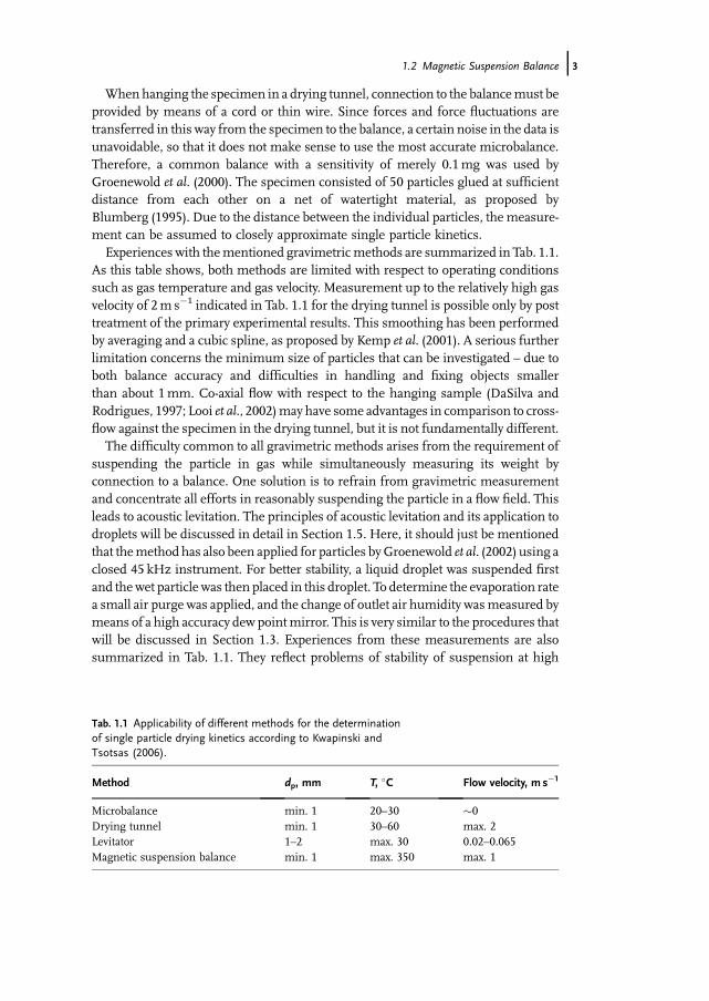
When hanging the specimen in a drying tunnel, connection to the balancemust beprovided by means of a cord or thin wire. Since forces and force fluctuations aretransferred in this way from the specimen to the balance, a certain noise in the data isunavoidable, so that it does not make sense to use the most accurate microbalance.Therefore, a common balance with a sensitivity of merely 0.1mg was used byGroenewold et al. (2000). The specimen consisted of 50 particles glued at sufficientdistance from each other on a net of watertight material, as proposed byBlumberg (1995). Due to the distance between the individual particles, the measure-ment can be assumed to closely approximate single particle kinetics.Experiences with thementioned gravimetricmethods are summarized in Tab. 1.1.

As this table shows, both methods are limited with respect to operating conditionssuch as gas temperature and gas velocity. Measurement up to the relatively high gasvelocity of 2m s�1 indicated in Tab. 1.1 for the drying tunnel is possible only by posttreatment of the primary experimental results. This smoothing has been performedby averaging and a cubic spline, as proposed by Kemp et al. (2001). A serious furtherlimitation concerns the minimum size of particles that can be investigated – due toboth balance accuracy and difficulties in handling and fixing objects smallerthan about 1mm. Co-axial flow with respect to the hanging sample (DaSilva andRodrigues, 1997; Looi et al., 2002)may have some advantages in comparison to cross-flow against the specimen in the drying tunnel, but it is not fundamentally different.The difficulty common to all gravimetric methods arises from the requirement of

suspending the particle in gas while simultaneously measuring its weight byconnection to a balance. One solution is to refrain from gravimetric measurementand concentrate all efforts in reasonably suspending the particle in a flow field. Thisleads to acoustic levitation. The principles of acoustic levitation and its application todroplets will be discussed in detail in Section 1.5. Here, it should just be mentionedthat themethod has also been applied for particles byGroenewold et al. (2002) using aclosed 45 kHz instrument. For better stability, a liquid droplet was suspended firstand thewet particle was then placed in this droplet. To determine the evaporation ratea small air purge was applied, and the change of outlet air humidity wasmeasured bymeans of a high accuracy dew pointmirror. This is very similar to the procedures thatwill be discussed in Section 1.3. Experiences from these measurements are alsosummarized in Tab. 1.1. They reflect problems of stability of suspension at high

Tab. 1.1 Applicability of different methods for the determinationof single particle drying kinetics according to Kwapinski andTsotsas (2006).

Method dp, mm T, �C Flow velocity, m s�1

Microbalance min. 1 20–30 �0Drying tunnel min. 1 30–60 max. 2Levitator 1–2 max. 30 0.02–0.065Magnetic suspension balance min. 1 max. 350 max. 1

1.2 Magnetic Suspension Balance j3

temperatures and strong purges, which would evidently destroy the oscillatingpressure field and, thus, also the suspension force acting on the particle.An alternative strategy is to still use a balance, but refrain from any material

connection between specimen andweightmeasuring cell. The realization of this ideain a magnetic suspension balance will be discussed in the following.

1.2.2Configuration and Periphery of Magnetic Suspension Balance

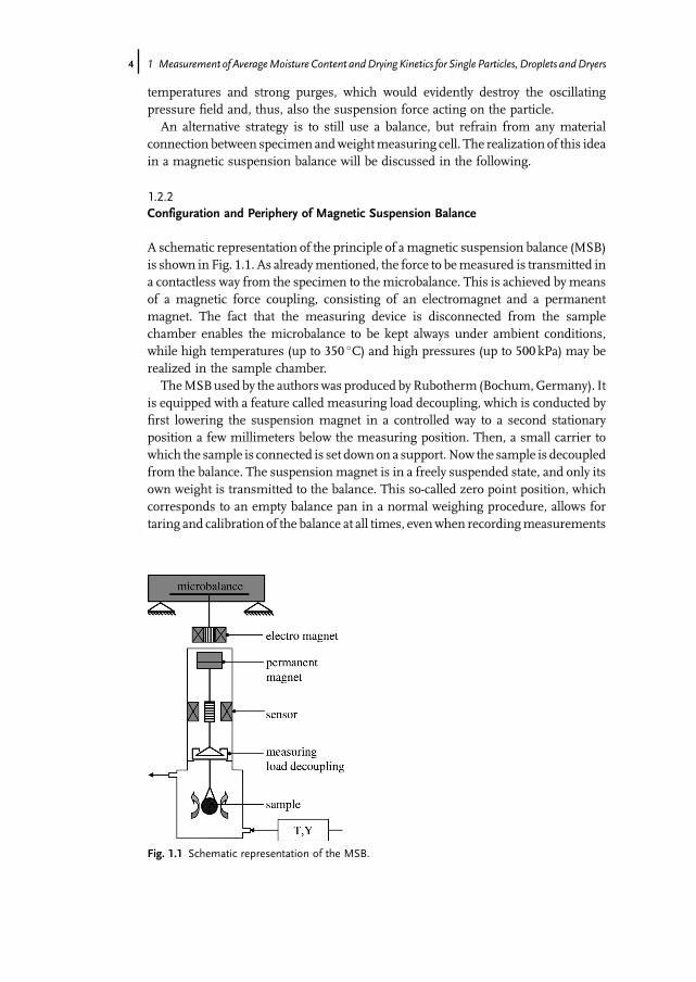
A schematic representation of the principle of amagnetic suspension balance (MSB)is shown in Fig. 1.1. As alreadymentioned, the force to bemeasured is transmitted ina contactless way from the specimen to the microbalance. This is achieved by meansof a magnetic force coupling, consisting of an electromagnet and a permanentmagnet. The fact that the measuring device is disconnected from the samplechamber enables the microbalance to be kept always under ambient conditions,while high temperatures (up to 350 �C) and high pressures (up to 500 kPa) may berealized in the sample chamber.TheMSBused by the authorswas produced by Rubotherm (Bochum,Germany). It

is equipped with a feature called measuring load decoupling, which is conducted byfirst lowering the suspension magnet in a controlled way to a second stationaryposition a few millimeters below the measuring position. Then, a small carrier towhich the sample is connected is set downon a support. Now the sample is decoupledfrom the balance. The suspension magnet is in a freely suspended state, and only itsown weight is transmitted to the balance. This so-called zero point position, whichcorresponds to an empty balance pan in a normal weighing procedure, allows fortaring and calibration of the balance at all times, evenwhen recordingmeasurements

Fig. 1.1 Schematic representation of the MSB.


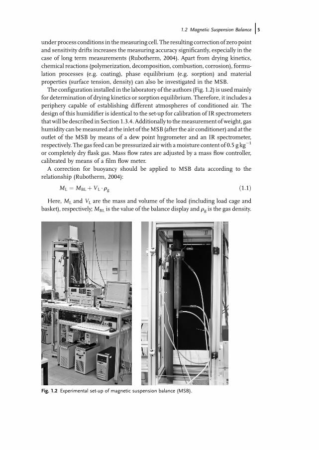
under process conditions in themeasuring cell. The resulting correction of zero pointand sensitivity drifts increases themeasuring accuracy significantly, especially in thecase of long term measurements (Rubotherm, 2004). Apart from drying kinetics,chemical reactions (polymerization, decomposition, combustion, corrosion), formu-lation processes (e.g. coating), phase equilibrium (e.g. sorption) and materialproperties (surface tension, density) can also be investigated in the MSB.The configuration installed in the laboratory of the authors (Fig. 1.2) is usedmainly

for determination of drying kinetics or sorption equilibrium. Therefore, it includes aperiphery capable of establishing different atmospheres of conditioned air. Thedesign of this humidifier is identical to the set-up for calibration of IR spectrometersthatwill be described in Section 1.3.4.Additionally to themeasurement ofweight, gashumidity can bemeasured at the inlet of theMSB (after the air conditioner) and at theoutlet of the MSB by means of a dew point hygrometer and an IR spectrometer,respectively. The gas feed can be pressurized air with amoisture content of 0.5 g kg�1

or completely dry flask gas. Mass flow rates are adjusted by a mass flow controller,calibrated by means of a film flow meter.A correction for buoyancy should be applied to MSB data according to the

relationship (Rubotherm, 2004):

ML ¼ MBL þVL � rg ð1:1ÞHere, ML and VL are the mass and volume of the load (including load cage and

basket), respectively;MBL is the value of the balance display and rg is the gas density.

Fig. 1.2 Experimental set-up of magnetic suspension balance (MSB).


Furthermore, for drying samples in the range of milligrams the buoyancy of thesample should be taken into account. Thus, the expression

MS ¼ MBLSðP;T ;wÞ�MBLðP;T ;wÞþVS � rgðP;T ;wÞ ð1:2Þcan be used to calculate the mass of the sample,MS. Here,MBLS is the value that thebalance displays with sample, MBL is the value that the balance displays withoutsample and VS is the volume of the dry sample. The influence of changing statevariables in the sample chamber (pressure P, temperature T, relative humidity w) isconsidered in Eq. 1.2. However, the buoyancy effect contributed by water (moisture),which is usually less than 1mg, is neglected.

1.2.3Discussion of Selected Experimental Results

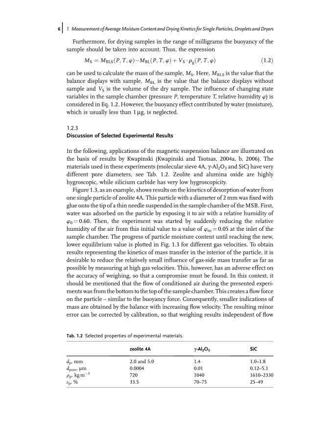
In the following, applications of the magnetic suspension balance are illustrated onthe basis of results by Kwapinski (Kwapinski and Tsotsas, 2004a, b, 2006). Thematerials used in these experiments (molecular sieve 4A, g -Al2O3 and SiC) have verydifferent pore diameters, see Tab. 1.2. Zeolite and alumina oxide are highlyhygroscopic, while silicium carbide has very low hygroscopicity.Figure 1.3, as an example, shows results on the kinetics of desorption ofwater from

one single particle of zeolite 4A. This particle with a diameter of 2mmwas fixed withglue onto the tip of a thin needle suspended in the sample chamber of theMSB. First,water was adsorbed on the particle by exposing it to air with a relative humidity ofw0¼ 0.60. Then, the experiment was started by suddenly reducing the relativehumidity of the air from this initial value to a value of win¼ 0.05 at the inlet of thesample chamber. The progress of particle moisture content until reaching the new,lower equilibrium value is plotted in Fig. 1.3 for different gas velocities. To obtainresults representing the kinetics of mass transfer in the interior of the particle, it isdesirable to reduce the relatively small influence of gas-side mass transfer as far aspossible by measuring at high gas velocities. This, however, has an adverse effect onthe accuracy of weighing, so that a compromise must be found. In this context, itshould be mentioned that the flow of conditioned air during the presented experi-mentswas from the bottom to the top of the sample chamber. This creates aflow forceon the particle – similar to the buoyancy force. Consequently, smaller indications ofmass are obtained by the balance with increasing flow velocity. The resulting minorerror can be corrected by calibration, so that weighing results independent of flow

Tab. 1.2 Selected properties of experimental materials.

zeolite 4A c-Al2O3 SiC

dp, mm 2.0 and 5.0 1.4 1.0–1.8dpore, mm 0.0004 0.01 0.12–5.1rp, kgm

�3 720 1040 1610–2330ep, % 33.5 70–75 25–49


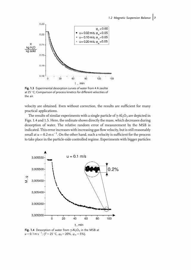
velocity are obtained. Even without correction, the results are sufficient for manypractical applications.The results of similar experiments with a single particle of g-Al2O3 are depicted in

Figs. 1.4 and 1.5. Here, the ordinate shows directly themass, which decreases duringdesorption of water. The relative random error of measurement by the MSB isindicated. This error increases with increasing gasflow velocity, but is still reasonablysmall at u¼ 0.2m s�1. On the other hand, such a velocity is sufficient for the processto take place in the particle-side controlled regime. Experiments with bigger particles

Fig. 1.3 Experimental desorption curves of water from 4 A zeoliteat 25 �C; Comparison of process kinetics for different velocities ofthe air.

Fig. 1.4 Desorption of water from g -Al2O3 in the MSB atu¼ 0.1m s�1; (T¼ 25 �C, w0¼ 20%, win¼ 5%).


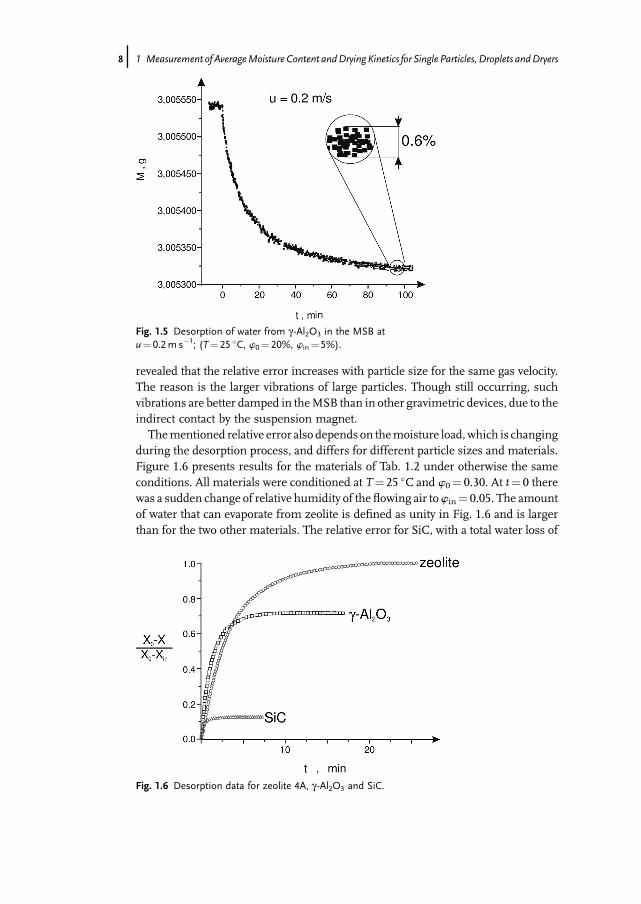
revealed that the relative error increases with particle size for the same gas velocity.The reason is the larger vibrations of large particles. Though still occurring, suchvibrations are better damped in theMSB than in other gravimetric devices, due to theindirect contact by the suspension magnet.Thementioned relative error also depends on themoisture load,which is changing

during the desorption process, and differs for different particle sizes and materials.Figure 1.6 presents results for the materials of Tab. 1.2 under otherwise the sameconditions. All materials were conditioned at T¼ 25 �C and w0¼ 0.30. At t¼ 0 therewas a sudden change of relative humidity of the flowing air towin¼ 0.05. The amountof water that can evaporate from zeolite is defined as unity in Fig. 1.6 and is largerthan for the two other materials. The relative error for SiC, with a total water loss of

Fig. 1.5 Desorption of water from g -Al2O3 in the MSB atu¼ 0.2m s�1; (T¼ 25 �C, w0¼ 20%, win¼ 5%).

Fig. 1.6 Desorption data for zeolite 4A, g -Al2O3 and SiC.


about 10 times less than zeolite, will be proportionally larger. This ratio is notconstant, but depends on the operating conditions. It should, however, be pointed outthat SiC is usually considered to be completely non-hygroscopic. In fact, the weakhygroscopicity indicated by Fig. 1.6 could not be detected by conventional gravimetricmethods, but can be detected in the MSB.Using the MSB it is also possible to gain equilibrium data. Examples of isotherms

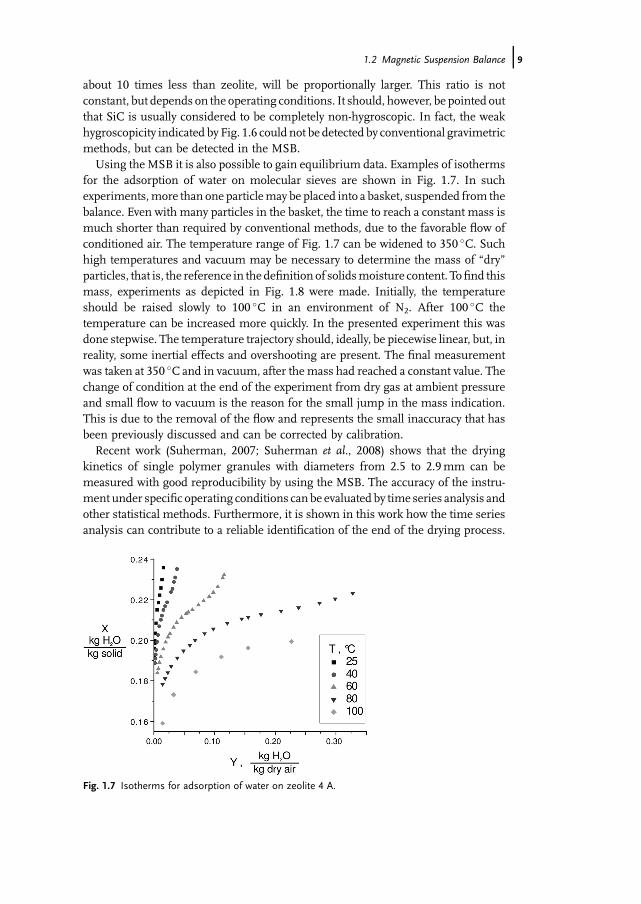
for the adsorption of water on molecular sieves are shown in Fig. 1.7. In suchexperiments,more than one particlemay be placed into a basket, suspended from thebalance. Even with many particles in the basket, the time to reach a constant mass ismuch shorter than required by conventional methods, due to the favorable flow ofconditioned air. The temperature range of Fig. 1.7 can be widened to 350 �C. Suchhigh temperatures and vacuum may be necessary to determine the mass of �dry�particles, that is, the reference in the definition of solidsmoisture content. Tofind thismass, experiments as depicted in Fig. 1.8 were made. Initially, the temperatureshould be raised slowly to 100 �C in an environment of N2. After 100 �C thetemperature can be increased more quickly. In the presented experiment this wasdone stepwise. The temperature trajectory should, ideally, be piecewise linear, but, inreality, some inertial effects and overshooting are present. The final measurementwas taken at 350 �C and in vacuum, after the mass had reached a constant value. Thechange of condition at the end of the experiment from dry gas at ambient pressureand small flow to vacuum is the reason for the small jump in the mass indication.This is due to the removal of the flow and represents the small inaccuracy that hasbeen previously discussed and can be corrected by calibration.Recent work (Suherman, 2007; Suherman et al., 2008) shows that the drying

kinetics of single polymer granules with diameters from 2.5 to 2.9mm can bemeasured with good reproducibility by using the MSB. The accuracy of the instru-ment under specific operating conditions canbe evaluated by time series analysis andother statistical methods. Furthermore, it is shown in this work how the time seriesanalysis can contribute to a reliable identification of the end of the drying process.

Fig. 1.7 Isotherms for adsorption of water on zeolite 4 A.


This helps to accurately determine dry mass. Statistical methods can also supportdata smoothing. Instead of the previouslymentioned cubic splines, Suherman (2007)used the moving average technique to this purpose. By smoothing the primary datathe significance of measurements can be extended towards smaller moisture con-tents at the end of the drying process.A coarse estimation of the applicability range of the MSB is given in Tab. 1.1.

Concerning this table, it should be noticed that the maximum operating velocity ofu¼ 2ms�1 assigned to the drying tunnel could be attained only in combination withnumerical smoothing of the primary data. In contrast, gas velocities of up tou¼ 1ms�1 can be realized in the MSB without smoothing. Without smoothing,the MSB has an advantage with regard to the maximum possible gas velocity.Nevertheless, such information is only indicative, because the applicability range

shrinks unavoidably with decreasing particle diameter, due to the decrease in weight.Additionally, it becomesmore andmore difficult tofix one particlewithout significantcontact with some solid support. Consequently, the applicability of all gravimetricmethods – including the MSB – ends at a particle diameter of about 1mm. Forpowdery materials with much smaller particle size alternative methods are needed.Such alternatives will be discussed in the following section.

1.3Infrared Spectroscopy and Dew Point Measurement

1.3.1Measurement for Particle Systems – General Remarks

As discussed in the previous section, the determination of the drying kinetics ofmaterials with a particle size below 1mm can hardly be conducted by single particleexperiments; the accuracy and resolution of the methods available for this purpose

Fig. 1.8 Measurement for the determination of the mass of dry zeolite by use of the MSB.


are not high enough. Consequently, it is necessary tomeasure the temporal change inmoisture content of an entire particle system and then extract from this informationsingle particle drying kinetics. The particle systems considered are packed beds andfluidized beds.The use of a packed bed corresponds to the well known thin layer method (TLM,

see, e.g. Hirschmann et al., 1998). In TLM a shallow packed bed is placed on a sievewith air flow in the direction of gravity. The moisture content of the packed bed ismeasured by interrupting the experiment and weighing. Alternatively, outlet gashumidity can be measured and used to calculate the corresponding change in themoisture content of the solids. Even for very thin layers the results of this methodcannot be set equal to single particle drying kinetics, but have to be scaled-down to thesingle particle by an appropriate model. Such modeling is not trivial, due to axialdispersion in the gas flowing through the packed bed. Additionally, it is difficult toprepare a particle layer of small but uniform thickness. Differences in thickness lead,however, to flow maldistribution, because the gas prefers pathways of minimal bedthickness and, thus, minimal flow resistance. Such flow bypasses can hardly bemodeled. Moreover, they depend on the skills of the person who has prepared andconducted the experiment.Gas bypass is also present in afluidized bed, due to bubbling.However, this bypass

is a property of the particle system – rather independent from the operator.Furthermore, reliable models are available for scaling fluidized bed drying resultsto the single particle. Because of these advantages, the route from fluidized bedmeasurements to single particle drying kinetics will be discussed in detail in thissection.The first step is the determination of the change in solids moisture content in the

fluidized bed with time. Conventionally, one takes samples out of the bed during thedrying process andmeasures themoisture content by weighing. This is intermittent,changes the hold-up and provides just a few points along the drying curve of thefluidized bed. Therefore, it is better to determine the decrease in solids moisturecontent in thefluidized beddryer indirectly, bymeasuring the gasmoisture content atthe outlet. For the simple case of a batch dryer one needs to quantify the moisturecontent of the gas at the inlet and at the outlet of the dryer and themassflow rate of thedry fluidization gas. The evaporation flow rate is then given by

_Mv ¼ _MgðYout�Y inÞ ð1:3Þ

Taking into account the initial moisture content of the solids X0, the temporalchange of moisture can be determined from

XðtÞ ¼ X0� 1Mdry

ð_MgðYout�Y inÞdt ð1:4Þ

Obviously, themeasurement of the gasmoisture contents Yout and Yin determinesthe quality of the method. Before discussing this measurement, by infrared spec-troscopy and dew point determination, a short outline of the experimental set-up willbe given.

1.3 Infrared Spectroscopy and Dew Point Measurement j11

1.3.2Experimental Set-Up

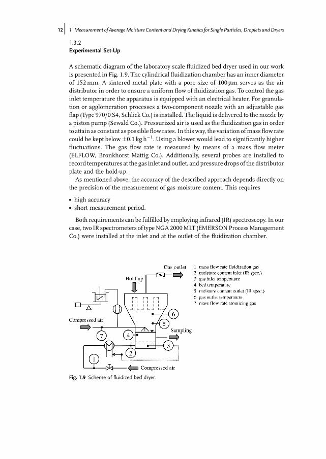
A schematic diagram of the laboratory scale fluidized bed dryer used in our workis presented in Fig. 1.9. The cylindrical fluidization chamber has an inner diameterof 152mm. A sintered metal plate with a pore size of 100 mm serves as the airdistributor in order to ensure a uniform flow of fluidization gas. To control the gasinlet temperature the apparatus is equipped with an electrical heater. For granula-tion or agglomeration processes a two-component nozzle with an adjustable gasflap (Type 970/0 S4, Schlick Co.) is installed. The liquid is delivered to the nozzle bya piston pump (Sewald Co.). Pressurized air is used as the fluidization gas in orderto attain as constant as possibleflow rates. In thisway, the variation ofmassflow ratecould be kept below�0.1 kg h�1. Using a blower would lead to significantly higherfluctuations. The gas flow rate is measured by means of a mass flow meter(ELFLOW, Bronkhorst M€attig Co.). Additionally, several probes are installed torecord temperatures at the gas inlet and outlet, and pressure drops of the distributorplate and the hold-up.As mentioned above, the accuracy of the described approach depends directly on

the precision of the measurement of gas moisture content. This requires

. high accuracy

. short measurement period.

Both requirements can be fulfilled by employing infrared (IR) spectroscopy. In ourcase, two IR spectrometers of typeNGA2000MLT (EMERSONProcessManagementCo.) were installed at the inlet and at the outlet of the fluidization chamber.

Fig. 1.9 Scheme of fluidized bed dryer.


1.3.3Principle of Measurement with the Infrared Spectrometer

The basis of IR spectroscopy is absorption of infrared radiation caused by the gasbeing measured. While the wavelengths of the absorption bands are specific to thetype of gas, the strength of absorption is a measure of concentration. By means of arotating chopper wheel, the radiation intensities coming from themeasuring and thereference sides of the cell of the instrument produce periodically changing signalswithin a detector. The detector signal amplitude thus alternates between concentra-tion dependent and concentration independent values. The difference between thetwo is a reliable measure of the concentration of the absorbing gas component.Figure 1.10 depicts a scheme of the IR spectrometer. A heating coil in the light

source (1) generates the necessary infrared radiation. This radiation passes throughthe light chopperwheel (2) and afilter cell (4) that screens interferingwavelengths outof the radiation spectrum.Due to the shape of the chopper wheel, irradiation of equalintensity alternates between the measuring side (6) and the reference side (7) of theanalysis cell (5). Only the measuring side is swept by the gas to be analyzed.Subsequently, the radiation passes individual optical filters around a second filtercell (8) and reaches the pyro-electrical detector (10). This detector compares themeasuring side radiation, which is reduced because of absorption by the gas, and the

Fig. 1.10 Scheme of IR spectrometer.


reference side radiation. Cooling and heating of the pyro-electrical material of thesensor lead to an alternating voltage signal. The final measuring signal of the IRspectrometer is equivalent to the volume concentration of the absorbing gascomponent. In our case, this component is water vapor. Volume concentration isequal to molar fraction ~y, which can be converted into the mass moisture content bythe relationship

Y ¼~Mw

~Mg

~y1�~y ð1:5Þ

1.3.4Dew Point Mirror for Calibration of IR Spectrometer

To achieve the highest precision for the determination of themoisture content in thegas phase the IR spectrometers need to be calibrated frequently since the pressure inthe measuring chamber and, therefore, also the measured volume concentration ofwater, depend on the ambient pressure. For the calibration, a gas flow with definedmoisture content must be supplied to the IR spectrometers. The accuracy ofcalibration of the spectrometers will depend directly on the accuracy of the measure-ment ofmoisture of the provided calibration gas. Dew pointmirrors are amongst themost established and recognized devices for the precise determination of moisturecontent in gases, because of their simplicity and the fundamental principle em-ployed. From themeasured dew point temperature Tdp, the saturation pressure p� ofthe water and hence the moisture content can be acquired:

Y ¼~Mw

~Mg

p�ðTdpÞP�p�ðTdpÞ ð1:6Þ

In a dew point instrument a gas sample is conducted into the sensor cell thatcontains a miniature temperature-controlled polished metal mirror (Fig. 1.11). This

Fig. 1.11 Operating principle of a dew point mirror.


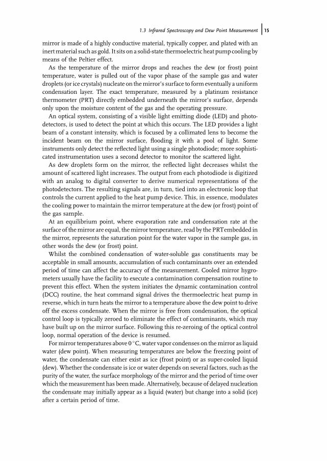
mirror is made of a highly conductive material, typically copper, and plated with aninertmaterial such as gold. It sits on a solid-state thermoelectric heat pumpcooling bymeans of the Peltier effect.As the temperature of the mirror drops and reaches the dew (or frost) point

temperature, water is pulled out of the vapor phase of the sample gas and waterdroplets (or ice crystals) nucleate on themirror�s surface to formeventually a uniformcondensation layer. The exact temperature, measured by a platinum resistancethermometer (PRT) directly embedded underneath the mirror�s surface, dependsonly upon the moisture content of the gas and the operating pressure.An optical system, consisting of a visible light emitting diode (LED) and photo-

detectors, is used to detect the point at which this occurs. The LED provides a lightbeam of a constant intensity, which is focused by a collimated lens to become theincident beam on the mirror surface, flooding it with a pool of light. Someinstruments only detect the reflected light using a single photodiode; more sophisti-cated instrumentation uses a second detector to monitor the scattered light.As dew droplets form on the mirror, the reflected light decreases whilst the

amount of scattered light increases. The output from each photodiode is digitizedwith an analog to digital converter to derive numerical representations of thephotodetectors. The resulting signals are, in turn, tied into an electronic loop thatcontrols the current applied to the heat pump device. This, in essence, modulatesthe cooling power to maintain the mirror temperature at the dew (or frost) point ofthe gas sample.At an equilibrium point, where evaporation rate and condensation rate at the

surface of themirror are equal, themirror temperature, read by the PRTembedded inthe mirror, represents the saturation point for the water vapor in the sample gas, inother words the dew (or frost) point.Whilst the combined condensation of water-soluble gas constituents may be

acceptable in small amounts, accumulation of such contaminants over an extendedperiod of time can affect the accuracy of the measurement. Cooled mirror hygro-meters usually have the facility to execute a contamination compensation routine toprevent this effect. When the system initiates the dynamic contamination control(DCC) routine, the heat command signal drives the thermoelectric heat pump inreverse, which in turn heats themirror to a temperature above the dew point to driveoff the excess condensate. When the mirror is free from condensation, the opticalcontrol loop is typically zeroed to eliminate the effect of contaminants, which mayhave built up on the mirror surface. Following this re-zeroing of the optical controlloop, normal operation of the device is resumed.Formirror temperatures above 0 �C,water vapor condenses on themirror as liquid

water (dew point). When measuring temperatures are below the freezing point ofwater, the condensate can either exist as ice (frost point) or as super-cooled liquid(dew).Whether the condensate is ice or water depends on several factors, such as thepurity of the water, the surface morphology of the mirror and the period of time overwhich themeasurement has beenmade. Alternatively, because of delayed nucleationthe condensate may initially appear as a liquid (water) but change into a solid (ice)after a certain period of time.


For water to freeze, the molecules must become properly aligned to each other, sothat it is more difficult to liberate a molecule from ice than from super-cooled liquidwater. Therefore, different saturation temperatures are measured for super-cooledwater and ice, the former being lower than the latter. This phenomenon affects allcooled mirror instruments and may result in inaccurate interpretation. If thecondensate present over a mirror is ice, the mirror temperature at equilibrium willbe higher than if the condensate were super-cooled liquid. The errors involved aretypically about 10% of water vapor pressure. In order to distinguish between waterand ice, some hygrometers are equipped with a microscope which allows the user tovisually inspect the surface of the mirror during measurement and look for frost ordew formation.However, the addition of amicroscope is usually an expensive option,and it can be difficult to discern water from ice formation, particularly at low dewpoint temperatures.In the present work an Optidew Vision (Michell Instruments Co.) dew point

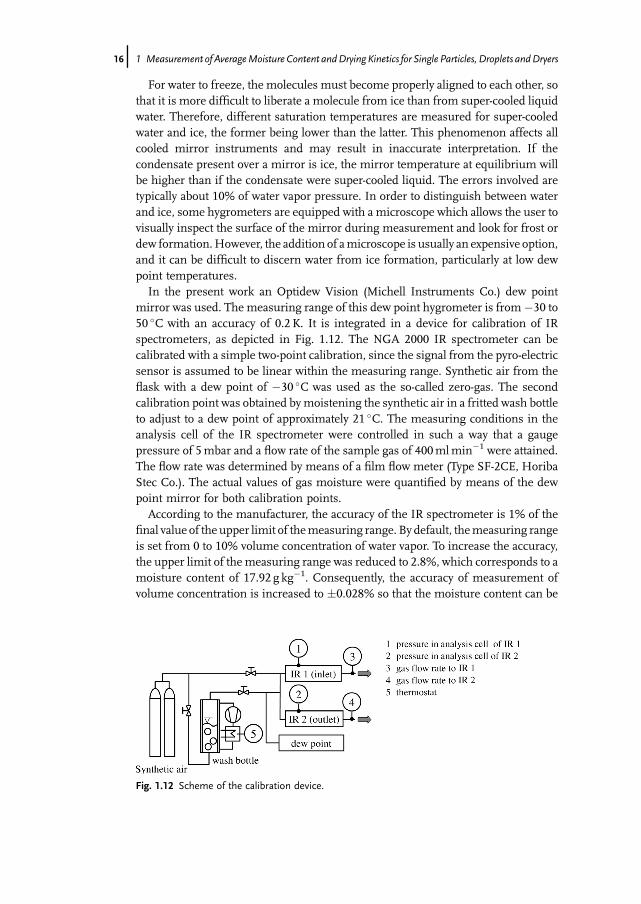
mirror was used. The measuring range of this dew point hygrometer is from�30 to50 �C with an accuracy of 0.2 K. It is integrated in a device for calibration of IRspectrometers, as depicted in Fig. 1.12. The NGA 2000 IR spectrometer can becalibrated with a simple two-point calibration, since the signal from the pyro-electricsensor is assumed to be linear within the measuring range. Synthetic air from theflask with a dew point of �30 �C was used as the so-called zero-gas. The secondcalibration point was obtained bymoistening the synthetic air in a fritted wash bottleto adjust to a dew point of approximately 21 �C. The measuring conditions in theanalysis cell of the IR spectrometer were controlled in such a way that a gaugepressure of 5mbar and a flow rate of the sample gas of 400mlmin�1 were attained.The flow rate was determined by means of a film flow meter (Type SF-2CE, HoribaStec Co.). The actual values of gas moisture were quantified by means of the dewpoint mirror for both calibration points.According to the manufacturer, the accuracy of the IR spectrometer is 1% of the

final value of the upper limit of themeasuring range. By default, themeasuring rangeis set from 0 to 10% volume concentration of water vapor. To increase the accuracy,the upper limit of the measuring range was reduced to 2.8%, which corresponds to amoisture content of 17.92 g kg�1. Consequently, the accuracy of measurement ofvolume concentration is increased to �0.028% so that the moisture content can be

Fig. 1.12 Scheme of the calibration device.


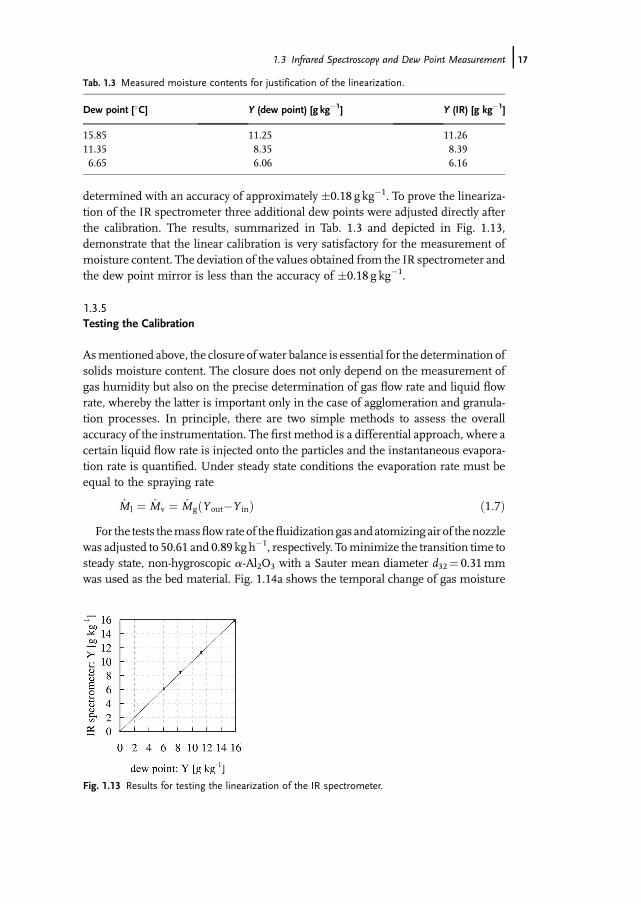
determined with an accuracy of approximately �0.18 g kg�1. To prove the lineariza-tion of the IR spectrometer three additional dew points were adjusted directly afterthe calibration. The results, summarized in Tab. 1.3 and depicted in Fig. 1.13,demonstrate that the linear calibration is very satisfactory for the measurement ofmoisture content. The deviation of the values obtained from the IR spectrometer andthe dew point mirror is less than the accuracy of �0.18 g kg�1.

1.3.5Testing the Calibration

Asmentioned above, the closure of water balance is essential for the determination ofsolids moisture content. The closure does not only depend on the measurement ofgas humidity but also on the precise determination of gas flow rate and liquid flowrate, whereby the latter is important only in the case of agglomeration and granula-tion processes. In principle, there are two simple methods to assess the overallaccuracy of the instrumentation. The first method is a differential approach, where acertain liquid flow rate is injected onto the particles and the instantaneous evapora-tion rate is quantified. Under steady state conditions the evaporation rate must beequal to the spraying rate

_Ml ¼ _Mv ¼ _MgðYout�Y inÞ ð1:7ÞFor the tests themassflowrate of thefluidizationgas andatomizing air of thenozzle

was adjusted to 50.61 and 0.89 kgh�1, respectively. Tominimize the transition time tosteady state, non-hygroscopic a-Al2O3 with a Sauter mean diameter d32¼ 0.31mmwas used as the bed material. Fig. 1.14a shows the temporal change of gas moisture

Tab. 1.3 Measured moisture contents for justification of the linearization.

Dew point [�C] Y (dew point) [g kg�1] Y (IR) [g kg�1]

15.85 11.25 11.2611.35 8.35 8.396.65 6.06 6.16

Fig. 1.13 Results for testing the linearization of the IR spectrometer.


obtained for the three different spraying rates which are summarized in Tab. 1.4. Theoccasional sharp decrease in outlet moisture content is caused by the switching of thepistons of the pump that feedswater to the nozzle.When this happens, the liquidflowis interrupted for 1 to 2 s, which is readily detected by the spectrometer. Figure 1.14bpresents the comparison of the actual spraying rate with the evaporation ratedetermined by applying Eq. 1.7. As one can see, the deviation is very low. Only forthe highest spraying rate was a slight systematic difference observed.To quantify the error of the differential balance, the deviation of spraying rate from

evaporation rate

D _Mv ¼ _Ml� _MgðYout�Y inÞ ð1:8Þis presented in Fig. 1.15 for undisturbed steady state conditions. As one can see, theerror of the differential balance is approximately�2mg s�1 for the first two sprayingrates, but increases slightly andbecomes systematic for the highest spraying rate. Theresulting deviations are summarized in Tab. 1.4. In total, it can be concluded that thedifferential balance is successfully closed, so that the instantaneous evaporation ratecan be determined with an accuracy of approximately �3%.The second approach for proving the quality of closure of the moisture balance is

an integral method. Here, a certain amount of liquid is sprayed onto pre-driedparticles so that the particle moisture content increases. After a certain time the

Fig. 1.14 Experimental results for testing the differential waterbalance at spraying rates of 0.082, 0.110 and 0.134 g s�1; (a)temporal change of gas moisture content; (b) comparison ofevaporation rate from the IR spectrometer with gravimetricallydetermined spraying rate.

Tab. 1.4 Maximal deviation of differential balance.

M_ l [mg s�1] DM_ v [mg s�1] Error [%]

82.08 �2 �2.43110.64 �2 �1.80134.23 þ4 þ2.97


spraying is shut down and the moisture is removed again from the particles. Gasoutlet humidity is detected during the entire process. By integral evaluation of thesesignals the total amount of evaporated water can easily be quantified:

MvðtÞ ¼ð

_MgðYout�Y inÞdt ð1:9Þ

For these trials the same test material was utilized as in the previous experiments.The spraying rate was adjusted to 0.13 g s�1. Results for two gas flow rates of 50.66and 30.15 kg h�1 are presented in Fig. 1.16 and Fig. 1.17, respectively. Diagram (a)depicts in each case the temporal change of gas moisture content while diagram (b)illustrates the deviation of integral moisture balance obtained from

DMv ¼ MlðtÞ�MvðtÞ ð1:10ÞThe evolution of gas moisture content reflects clearly the pre-drying, the spraying

and the drying periods. Since the gasmass flow rate was reduced for the second trial,

Fig. 1.15 Calculated deviation of differential moisture balance.

Fig. 1.16 Experimental results for proving the integral waterbalance at a gas mass flow rate of 50.66 kg h�1; (a) temporalchange of gasmoisture content; (b) deviation of cumulative massof water.


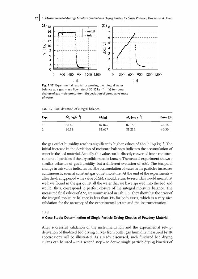
the gas outlet humidity reaches significantly higher values of about 16 g kg�1. Theinitial increase in the deviation of moisture balances indicates the accumulation ofwater in the bedmaterial. Actually, this value can be directly converted into amoisturecontent of particles if the dry solids mass is known. The second experiment shows asimilar behavior of gas humidity, but a different evolution of DMv. The temporalchange in this value indicates that the accumulation ofwater in the particles increasescontinuously, even at constant gas outlet moisture. At the end of the experiments –after the drying period – the value ofDMv should return to zero. This wouldmean thatwe have found in the gas outlet all the water that we have sprayed into the bed andwould, thus, correspond to perfect closure of the integral moisture balance. Themeasured final values ofDMv are summarized in Tab. 1.5. They show that the error ofthe integral moisture balance is less than 1% for both cases, which is a very nicevalidation for the accuracy of the experimental set-up and the instrumentation.

1.3.6A Case Study: Determination of Single Particle Drying Kinetics of Powdery Material

After successful validation of the instrumentation and the experimental set-up,derivation of fluidized bed drying curves from outlet gas humidity measured by IRspectroscopy will be illustrated. As already discussed, such fluidized bed dryingcurves can be used – in a second step – to derive single particle drying kinetics of

Fig. 1.17 Experimental results for proving the integral waterbalance at a gas mass flow rate of 30.15 kg h�1; (a) temporalchange of gasmoisture content; (b) deviation of cumulativemassof water.

Tab. 1.5 Final deviation of integral balance.

Exp. M_ g [kg h�1] Ml [g] Mv [mg s�1] Error [%]

1 50.66 82.026 82.156 �0.162 30.15 81.627 81.219 þ0.50


powdery materials, which is not accessible directly because of their too small particlediameter.To this purpose, drying experiments were conducted with powdery polymer

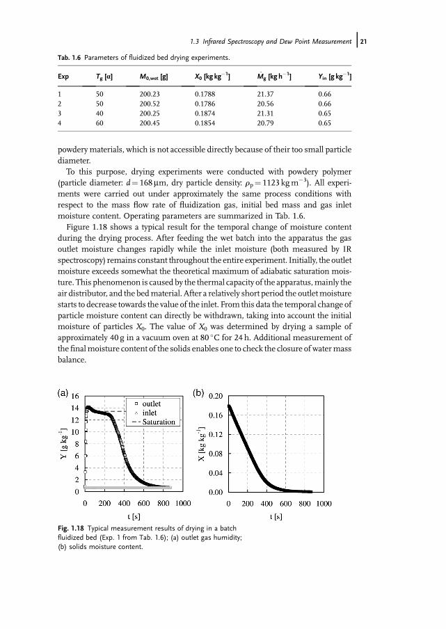
(particle diameter: d¼ 168mm, dry particle density: rp¼ 1123 kgm�3). All experi-ments were carried out under approximately the same process conditions withrespect to the mass flow rate of fluidization gas, initial bed mass and gas inletmoisture content. Operating parameters are summarized in Tab. 1.6.Figure 1.18 shows a typical result for the temporal change of moisture content

during the drying process. After feeding the wet batch into the apparatus the gasoutlet moisture changes rapidly while the inlet moisture (both measured by IRspectroscopy) remains constant throughout the entire experiment. Initially, the outletmoisture exceeds somewhat the theoretical maximum of adiabatic saturation mois-ture. This phenomenon is caused by the thermal capacity of the apparatus,mainly theair distributor, and the bedmaterial. After a relatively short period the outletmoisturestarts to decrease towards the value of the inlet. From this data the temporal change ofparticle moisture content can directly be withdrawn, taking into account the initialmoisture of particles X0. The value of X0 was determined by drying a sample ofapproximately 40 g in a vacuum oven at 80 �C for 24 h. Additional measurement ofthefinalmoisture content of the solids enables one to check the closure of watermassbalance.

Tab. 1.6 Parameters of fluidized bed drying experiments.

Exp Tg [a] M0,wet [g] X0 [kg kg�1] M_ g [kg h

�1] Yin [g kg�1]

1 50 200.23 0.1788 21.37 0.662 50 200.52 0.1786 20.56 0.663 40 200.25 0.1874 21.31 0.654 60 200.45 0.1854 20.79 0.65

Fig. 1.18 Typical measurement results of drying in a batchfluidized bed (Exp. 1 from Tab. 1.6); (a) outlet gas humidity;(b) solids moisture content.


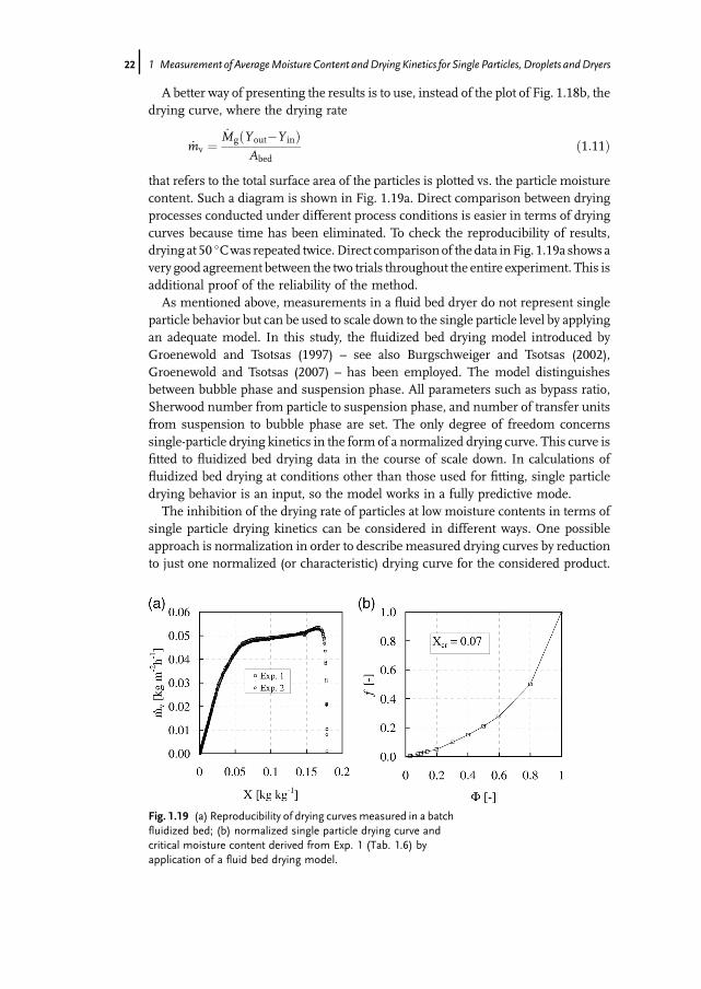
A better way of presenting the results is to use, instead of the plot of Fig. 1.18b, thedrying curve, where the drying rate

_mv ¼_MgðYout�Y inÞ

Abedð1:11Þ

that refers to the total surface area of the particles is plotted vs. the particle moisturecontent. Such a diagram is shown in Fig. 1.19a. Direct comparison between dryingprocesses conducted under different process conditions is easier in terms of dryingcurves because time has been eliminated. To check the reproducibility of results,drying at 50 �Cwas repeated twice.Direct comparison of the data in Fig. 1.19a shows avery good agreement between the two trials throughout the entire experiment. This isadditional proof of the reliability of the method.As mentioned above, measurements in a fluid bed dryer do not represent single

particle behavior but can be used to scale down to the single particle level by applyingan adequate model. In this study, the fluidized bed drying model introduced byGroenewold and Tsotsas (1997) – see also Burgschweiger and Tsotsas (2002),Groenewold and Tsotsas (2007) – has been employed. The model distinguishesbetween bubble phase and suspension phase. All parameters such as bypass ratio,Sherwood number from particle to suspension phase, and number of transfer unitsfrom suspension to bubble phase are set. The only degree of freedom concernssingle-particle drying kinetics in the form of a normalized drying curve. This curve isfitted to fluidized bed drying data in the course of scale down. In calculations offluidized bed drying at conditions other than those used for fitting, single particledrying behavior is an input, so the model works in a fully predictive mode.The inhibition of the drying rate of particles at low moisture contents in terms of

single particle drying kinetics can be considered in different ways. One possibleapproach is normalization in order to describe measured drying curves by reductionto just one normalized (or characteristic) drying curve for the considered product.

Fig. 1.19 (a) Reproducibility of drying curves measured in a batchfluidized bed; (b) normalized single particle drying curve andcritical moisture content derived from Exp. 1 (Tab. 1.6) byapplication of a fluid bed drying model.


This method was introduced for normalization of drying curves measured in batchdrying by van Meel (1958), and since then it has been applied in the original or inmodified formsbymany authors (vanBrakel, 1980; Shibata, 2005;Groenewold, 2004).The normalized drying rate f is defined as the quotient of the actual drying rate _mv,and the drying rate of the first drying period _m v;I

f ¼ _mv

_m v;Ið1:12Þ

and the normalized solids moisture content, F, is represented by

F ¼ X�X eq

X cr�X eqð1:13Þ

where Xeq is the equilibriummoisture content. Both f andF take values between 0and 1.Remember that drying is assumed to be gas-side controlled in the first and particle-

side controlled in the second drying period (at X<Xcr). By normalization the twoperiods are separated from each other. Gas-side phenomena (i.e. the drying rate _mv;I)are supposed to be predictable from first principles. Particle-side phenomena aredescribedempiricallyby thefunction f(F). Successfulnormalization leads toa functionf(F) which is invariant with drying conditions (Tsotsas, 1994; Suherman et al., 2008).Applying this concept, the normalized drying curve of a single particle aswell as the

critical moisture content are derived by scaling down from measurement results byiterative adjustment in a computer program that implements thefluidizedbed dryingmodel. For this derivation the data from experiment 1 (Tab. 1.6) has been used. Thenormalized drying curve is presented graphically in Fig. 1.19b, with a criticalmoisture content of Xcr¼ 0.07 for this product.Figure 1.20 illustrates the opposite exercise, by comparing calculations conducted

with thenormalized drying curve that has been derived fromone experimentwith the

Fig. 1.20 Comparison between measured and calculatedfluidized bed drying curves at different temperatures.


results of three fluidized bed experiments carried out at different gas inlet tempera-tures. The results show that at high moisture content the measured drying rate ishigher than the calculated one. As mentioned above, this is a thermal effect mainlycaused by the supply of heat to the fluidized bed from the equipment, in particularfrom the distributor plate. Before every drying experiment, the entire apparatus iswarmed to the inlet gas temperature. After the start of the experiment, heat transfertakes place between the equipment and the drying gas and/or the equipment and theparticles, since both the average gas temperature and the particle temperature areclearly lower than the gas inlet temperature in the first drying period. As a result ofthis additional energy, drying rates increase. Towards the end of the drying process,the drying rate reaches very small values, which are still determined from thedifference between the outlet and inlet gas humidities. Since the respectivemeasuredquantities become almost identical and exhibit a certain noise, scatter of the dryingrates is unavoidable at low moisture contents. Nevertheless, the derivation of dryingrates appears to be accurate enough till solids moisture contents of about 0.002 inthe present experiments.In spite of such restrictions, Fig. 1.20 shows quite good agreement between

measurement and simulation in the significant range of moisture content. This istrue, in particular, for the influence of temperature. Consequently, the concept ofnormalization works well for the present example. This is not always the case(Suherman et al., 2008), so that it may be better to use, for example, some diffusionmodel instead of the normalization method for other products. Then, diffusioncoefficients will be the quantities to determine by fitting of the fluidized bed dryingmodel to the experimental results. Apart from this, the described procedure remainsessentially the same.

1.4Coulometry and Nuclear Magnetic Resonance

1.4.1Particle Moisture as a Distributed Property

In this section, we address the problem of measuring the relatively low moisturecontent of a large number of particles on an individual basis with the necessaryprecision. This problem arises when particulate material is dried and particlemoisture at the outlet of the dryer is not uniform. In such a case, the characteristicsof the distribution of particle moisture decide the quality of the drying process. Ingeneral, the outlet moisture content of any product must be below some specifiedvalue for quality reasons, but over-drying is undesirable because of energy costs,capacity restrictions or product damage. In the following, we choose the example of acontinuous fluidized bed dryer (as sketched in Fig. 1.21) to illustrate, first, how themoisture content distribution may be approximated by a simplified populationbalancemodel and, then, how it can bemeasured. Subsequently, measuredmoisturedistributions will be compared with the model.


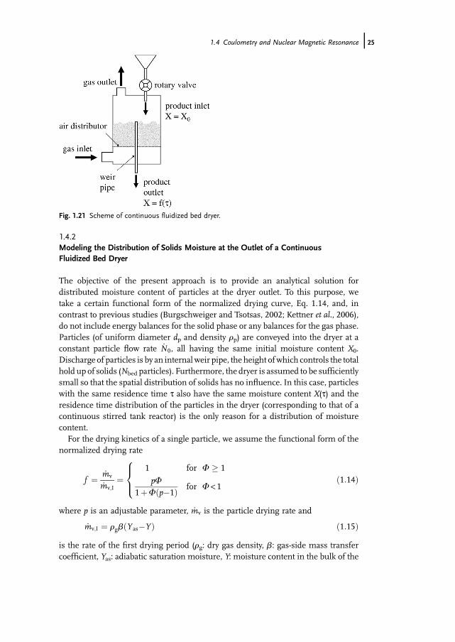
1.4.2Modeling the Distribution of Solids Moisture at the Outlet of a ContinuousFluidized Bed Dryer

The objective of the present approach is to provide an analytical solution fordistributed moisture content of particles at the dryer outlet. To this purpose, wetake a certain functional form of the normalized drying curve, Eq. 1.14, and, incontrast to previous studies (Burgschweiger and Tsotsas, 2002; Kettner et al., 2006),do not include energy balances for the solid phase or any balances for the gas phase.Particles (of uniform diameter dp and density rp) are conveyed into the dryer at aconstant particle flow rate _N0, all having the same initial moisture content X0.Discharge of particles is by an internalweir pipe, the height ofwhich controls the totalhold up of solids (Nbed particles). Furthermore, the dryer is assumed to be sufficientlysmall so that the spatial distribution of solids has no influence. In this case, particleswith the same residence time t also have the same moisture content X(t) and theresidence time distribution of the particles in the dryer (corresponding to that of acontinuous stirred tank reactor) is the only reason for a distribution of moisturecontent.For the drying kinetics of a single particle, we assume the functional form of the

normalized drying rate

f ¼ _mv

_mv;I¼

1 for F � 1

pF1þFðp�1Þ for F < 1

8><>: ð1:14Þ

where p is an adjustable parameter, _mv is the particle drying rate and

_mv;I ¼ rgbðYas�YÞ ð1:15Þis the rate of the first drying period (rg: dry gas density, b: gas-side mass transfercoefficient, Yas: adiabatic saturation moisture, Y: moisture content in the bulk of the

Fig. 1.21 Scheme of continuous fluidized bed dryer.

1.4 Coulometry and Nuclear Magnetic Resonance j25

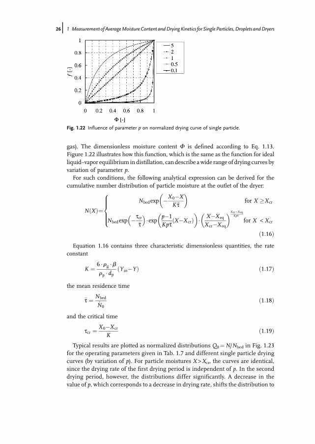
gas). The dimensionless moisture content F is defined according to Eq. 1.13.Figure 1.22 illustrates how this function, which is the same as the function for idealliquid–vapor equilibrium indistillation, can describe awide range of drying curves byvariation of parameter p.For such conditions, the following analytical expression can be derived for the

cumulative number distribution of particle moisture at the outlet of the dryer:

NðXÞ¼Nbedexp �X 0�X

Kt�

� �for X �X cr

Nbedexp �tcrt�

� ��exp p�1

Kpt�ðX�X crÞ

� �� X�X eq

X cr�X eq

� �Xcr�XeqKpt�

for X < X cr

8>>><>>>:

ð1:16ÞEquation 1.16 contains three characteristic dimensionless quantities, the rate

constant

K ¼ 6 � rg �brp � dp

ðYas�YÞ ð1:17Þ

the mean residence time

t�¼ Nbed

_N0ð1:18Þ

and the critical time

tcr ¼ X0�X cr

Kð1:19Þ

Typical results are plotted as normalized distributions Q0¼N/Nbed in Fig. 1.23for the operating parameters given in Tab. 1.7 and different single particle dryingcurves (by variation of p). For particle moistures X >Xcr, the curves are identical,since the drying rate of the first drying period is independent of p. In the seconddrying period, however, the distributions differ significantly. A decrease in thevalue of p, which corresponds to a decrease in drying rate, shifts the distribution to

Fig. 1.22 Influence of parameter p on normalized drying curve of single particle.


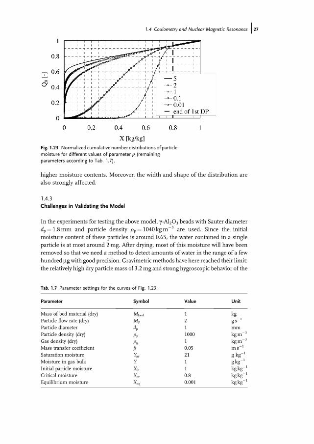
higher moisture contents. Moreover, the width and shape of the distribution arealso strongly affected.

1.4.3Challenges in Validating the Model

In the experiments for testing the above model, g -Al2O3 beads with Sauter diameterdp¼ 1.8mm and particle density rp¼ 1040 kgm�3 are used. Since the initialmoisture content of these particles is around 0.65, the water contained in a singleparticle is at most around 2mg. After drying, most of this moisture will have beenremoved so that we need a method to detect amounts of water in the range of a fewhundred mg with good precision. Gravimetricmethods have here reached their limit:the relatively high dry particle mass of 3.2mg and strong hygroscopic behavior of the

Fig. 1.23 Normalized cumulative number distributions of particlemoisture for different values of parameter p (remainingparameters according to Tab. 1.7).

Tab. 1.7 Parameter settings for the curves of Fig. 1.23.

Parameter Symbol Value Unit

Mass of bed material (dry) Mbed 1 kgParticle flow rate (dry) _Mp 2 g s�1

Particle diameter dp 1 mmParticle density (dry) rp 1000 kgm�3

Gas density (dry) rg 1 kgm�3

Mass transfer coefficient b 0.05 m s�1

Saturation moisture Yas 21 g kg�1

Moisture in gas bulk Y 1 g kg�1

Initial particle moisture X0 1 kg kg�1

Critical moisture Xcr 0.8 kg kg�1

Equilibrium moisture Xeq 0.001 kg kg�1


material (leading to significant moisture uptake during weighing) prevent anaccurate measurement of moisture content.When searching for an appropriate measurement method, we also have to bear in

mind that a sufficient number of particles (at least 100) have to be characterized for areliable comparison of experimental and theoretical distribution functions.In the following, we present the methods of coulometry and nuclear magnetic

resonance;wewill see, by analysis of their advantages anddisadvantages, that a combina-tion of both techniques is suitable for fast and accurate moisture measurements.

1.4.4Coulometry

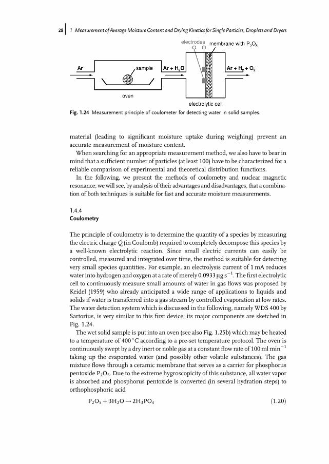
The principle of coulometry is to determine the quantity of a species by measuringthe electric chargeQ (in Coulomb) required to completely decompose this species bya well-known electrolytic reaction. Since small electric currents can easily becontrolled, measured and integrated over time, the method is suitable for detectingvery small species quantities. For example, an electrolysis current of 1mA reduceswater into hydrogen and oxygen at a rate ofmerely 0.0933mg s�1. Thefirst electrolyticcell to continuously measure small amounts of water in gas flows was proposed byKeidel (1959) who already anticipated a wide range of applications to liquids andsolids if water is transferred into a gas stream by controlled evaporation at low rates.The water detection system which is discussed in the following, namelyWDS 400 bySartorius, is very similar to this first device; its major components are sketched inFig. 1.24.The wet solid sample is put into an oven (see also Fig. 1.25b) whichmay be heated

to a temperature of 400 �C according to a pre-set temperature protocol. The oven iscontinuously swept by a dry inert or noble gas at a constant flow rate of 100mlmin�1

taking up the evaporated water (and possibly other volatile substances). The gasmixture flows through a ceramic membrane that serves as a carrier for phosphoruspentoxide P2O5. Due to the extreme hygroscopicity of this substance, all water vaporis absorbed and phosphorus pentoxide is converted (in several hydration steps) toorthophosphoric acid

P2O5 þ 3H2O! 2H3PO4 ð1:20Þ

Fig. 1.24 Measurement principle of coulometer for detecting water in solid samples.


Gas components other than water will pass through the membrane withoutreaction. Voltage is applied to the membrane by two electrodes (printed on itssurface) to dissociate the phosphoric acids, the final step of the respective anodic andcathodic reactions being

4PO�3 ! 2P2O5 þO2 þ 4e�

4Hþþ 4e� ! 2H2ð1:21Þ

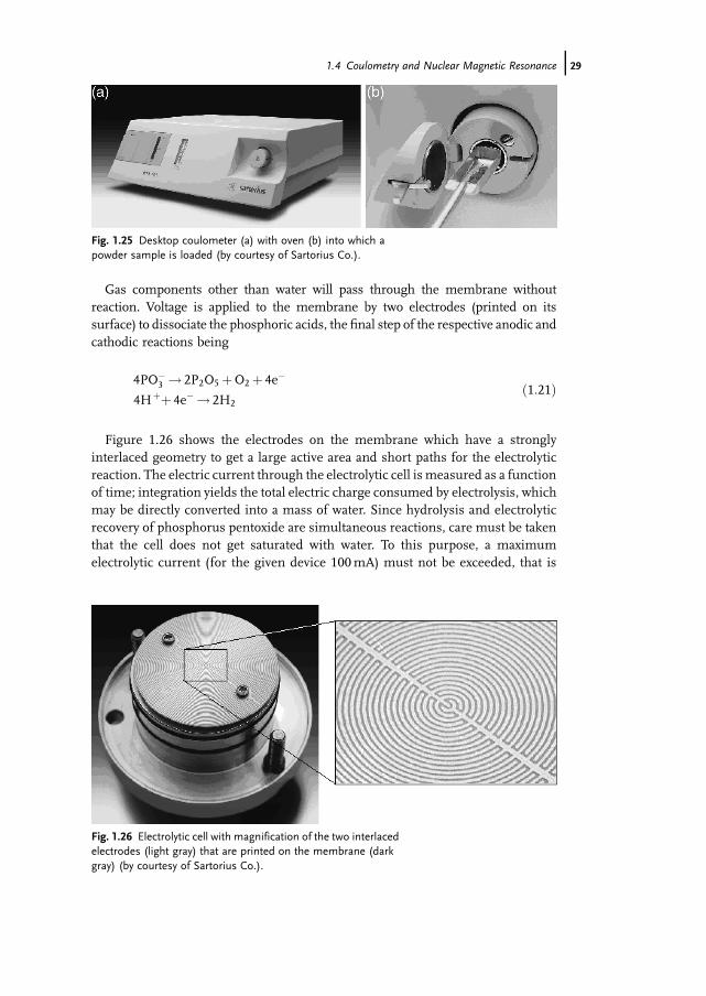
Figure 1.26 shows the electrodes on the membrane which have a stronglyinterlaced geometry to get a large active area and short paths for the electrolyticreaction. The electric current through the electrolytic cell is measured as a functionof time; integration yields the total electric charge consumed by electrolysis, whichmay be directly converted into a mass of water. Since hydrolysis and electrolyticrecovery of phosphorus pentoxide are simultaneous reactions, care must be takenthat the cell does not get saturated with water. To this purpose, a maximumelectrolytic current (for the given device 100mA) must not be exceeded, that is

Fig. 1.25 Desktop coulometer (a) with oven (b) into which apowder sample is loaded (by courtesy of Sartorius Co.).

Fig. 1.26 Electrolytic cell with magnification of the two interlacedelectrodes (light gray) that are printed on the membrane (darkgray) (by courtesy of Sartorius Co.).


water vapor must not be produced in the oven at too high rates (at a maximum9.3 mg s�1). On the other hand, too low electrolytic currents – associatedwith too lowevaporation rates – will be measured with a higher relative error so that watercontent is obtained at lower precision (integration over time has no effect on theerror). In conclusion, best results are obtained for elevated but not too highevaporation rates (here several mg s�1).It should be noted that the value of the electrolytic voltage is not critical as long as it

is well above 2 V, which is the decomposition voltage of water (Keidel, 1959).The efficiency of the cell depends on impurities and is regularly assessed by

calibration measurements with a well-defined amount of water. Since free waterwould evaporate too rapidly and lead to an overload of the detector, a standardsubstance, sodiumwolframate containing crystallinewater (Na2WO4�2H2O), is used;typically, 20–25mg of standard substance (with 1.07% water) are used. If theefficiency is too low, the electrolytic cell has to be refreshed by cleaning with waterand coating with an acetone solution of 85% orthophosphoric acid (H3PO4). Beforeperforming the next analysis measurement, the cell must be dried and the acidconverted into phosphorus pentoxide by electrolysis. The dehydration will, however,not be complete (HPO3 is considered the prevailing component) since the cellbecomes an insulator with increasing concentrations of P2O5 (Keidel, 1959).For quantitative analysis of water in solid samples, the following procedure is

applied:

1. Open the oven door and insert the sample scoop2. Close the oven door (a short time interval later)3. Heat the oven according to a pre-set temperature protocol4. Measure and integrate the electrolysis current over a given time interval.

It is obvious that such a measurement will not only detect the water from thesample, but also residual moisture in the flow of carrier gas andmoisture that entersthe system when opening the oven door; (recall that saturated air at 20 �C contains17.3mgml�1 water vapor and the total oven volume is 26ml). From this, it is obviousthat tare measurements without a solid sample are of paramount importance ifsmall solids moisture contents are to be quantified. Such a tare measurement has tobe done directly before quantitative analysis to account for changes of relativehumidity in ambient air; furthermore, exactly the same procedure has to be respectedas in the subsequent analytic measurements, that is same open time of oven, sametemperature protocol and measurement duration.Wewill now return to our task of characterizing particles fromafluidized bed dryer

with respect to their moisture content, which corresponds to measuring wateramounts in the range 100–2500mg. Recalling that the temperature protocol ideallyhas to be chosen so as to evaporatewater from the sample at a rate of severalmg s�1,wewill apply two different protocols. The first, which is applied to particles with ratherlowmoisture, accomplishes a temperature increase to 130 �C in one step and in totaltakes 10min (see Fig. 1.27a). The second is intended for larger amounts of water; inorder to prevent too high release rates, an intermediate temperature of 60 �C is firstassumed before heating to 130 �C in a second step; overall measurement duration is


14min (see Fig. 1.28a). To obtain reproducible results, argon (99.998 vol.%) at a flowrate of approximately 100mlmin�1 is used as a dry carrier gas in all measurements.Taremeasurements of electrolysis current for the two chosen temperature protocols

are given in Fig. 1.29. One may assume a constant background level that originatesfrom residual moisture in argon (a gas flow of 100mlmin�1 with 0.002 vol.% watervapor corresponds to a vapor flow of 1.48mgmin�1 or an electric current of 0.26mA).The different durations of the two protocols result in different contributions fromargon to the total detected moisture (14.8 and 20.7mg for protocols 1 and 2,respectively).The signal above this background results from the moisture entering the oven

during (sample) loading. Its shape depends slightly on the chosen temperatureprotocol but not its integral value (39.8 and 39.5mg for protocols 1 and 2, respectively).In this light, wemay understand the detection limit of the device that is given as 1mg.In the following, five samples (A–E) with increasing moisture content are charac-

terized. The completemeasurement results are given for the driest and for thewettestsample in Figs. 1.27 and 1.28, respectively. In Figs. 1.27a and 1.28a the oventemperature is plotted along with the value set by the protocol. Figures 1.27b and1.28b show the electrolysis current which is corrected by the tare measurement.

Fig. 1.27 (a) Temperature protocol and (b) electrolysis current fora particle with low moisture content (Mw¼ 161mg, sample A).

Fig. 1.28 (a) Temperature protocol and (b) electrolysis currentfor aparticlewithhighmoisture content (Mw¼ 2171mg, sampleE).


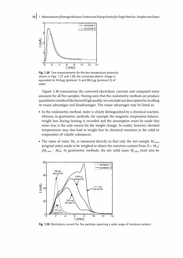
Figure 1.30 summarizes the corrected electrolysis currents and computed wateramounts for all five samples. Having seen that the coulometric method can producequantitative resultsof thedesiredhighquality,weconcludeourdescriptionbyrecallingits major advantages and disadvantages. The major advantages may be listed as:

. In the coulometric method, water is clearly distinguished by a chemical reaction,whereas in gravimetric methods, for example the magnetic suspension balance,weight loss during heating is recorded and the assumption must be made thatwater loss is the only reason for the weight change. In reality, however, elevatedtemperatures may also lead to weight loss by chemical reactions in the solid orevaporation of volatile substances.

. The mass of water Mw is measured directly so that only the wet sample Ms,wet

(original state) needs to be weighed to obtain the moisture content from X¼Mw/(Ms,wet�Mw). In gravimetric methods, the dry solid mass Ms,dry must also be

Fig. 1.29 Tare measurements for the two temperature protocolsshown in Figs. 1.27 and 1.28; the converted electric charge isequivalent to 54.6mg (protocol 1) and 60.2mg (protocol 2) ofwater.

Fig. 1.30 Electrolysis current for five particles spanning a wide range of moisture content.


measured to compute the moisture content as X¼ (Ms,wet�Ms,dry)/Ms,dry. Thisbrings the problem of removing all water without any other changes to thesample. Furthermore, in the case of low moisture contents, the weight differenceMs,wet�Ms,dry cannot be measured accurately due to limited balance precision,and this may reflect in a large error in X.

. The coulometric method may also be used for a rough quantitative distinction ofsurface water, capillary water and the more tightly bound water of crystallization ifthe temperature rise is performed in appropriate steps.

The major disadvantages of the coulometric method are:

. The sample as defined by a porous structure containing a certain amount ofwater isdestroyed so that the measurement cannot be repeated.

. Sample water content and release behavior of the water must be known approxi-mately so as to choose the optimal temperature protocol: on the one hand, theelectrolytic cell must not get saturated; on the other hand, the release rate shouldnot be too low so as to keep the measurement period short (see above). Whenlooking at the stochastic behavior of particles in a continuous fluidized bed dryer,such information is not available!

. The measurement of one sample takes a relatively long time (about 20min). Ifmany samples need to be measured to describe stochastic behavior, this is a severedrawback.

. The humidity of a relatively big gas volume (oven) needs to be corrected in a taremeasurement.

1.4.5Nuclear Magnetic Resonance

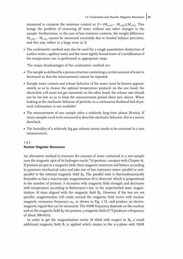
An alternative method to measure the amount of water contained in a wet sampleuses themagnetic spin of its hydrogen nuclei 1H (protons, compare with Chapter 4).If protons are put in amagnetic field, theirmagnetic moments will behave accordingto quantum mechanical rules and take one of two stationary states: parallel or anti-parallel to the external magnetic field B0. The parallel state is thermodynamicallyfavorable so that a macroscopic magnetizationM is observed, which is proportionalto the number of protons; it increases with magnetic field strength and decreaseswith temperature according to Boltzmann�s law. In the unperturbed state, magne-tization M stays aligned with the magnetic field B0. However, if the two are notparallel, magnetization will rotate around the magnetic field vector with nuclearmagnetic resonance frequency v0, as shown in Fig. 1.31, and produce an electro-magnetic signal that can be measured. The NMR frequency depends on the nucleusand on themagnetic fieldB0; for protons, amagnetic field of 7Tproduces a frequencyof about 300MHz.In order to get the magnetization vector M tilted with respect to B0, a small

additional magnetic field B1 is applied which rotates in the x–y-plane with NMR


frequency v0. By adjusting the magnitude of B1 and the pulse duration, the flippingangle can be tuned to 90�, which will produce the highest resonance signal. Inpractice, the same electromagnetic coil first produces the rotating B1-field and then(after a short dead time) measures the signal of the rotating M-vector. This NMRsignal decays with the so-called transverse relaxation time T2 because the rotatingprotons get out of phase due to small variations of NMR frequency in time and space;in consequence, the component of M orthogonal to the z-axis becomes zero. On alonger time scale (characterized by longitudinal relaxation time T1), the magnetiza-tion will relax back to its equilibrium state, that is parallel to B0.This type of NMR measurement is referred to as free induction decay (FID)

because the protonsmay relax after the initial pulsewithout further perturbation. Theinitial magnitude of the FID signal is proportional to the number of protons.However, the signal of adsorbed water decays faster than that of free water becauseof its strong interaction with the solid (Metzger et al., 2005). This is one reason whythe overall signal does not decay exponentially.Experiments on the wet g -Al2O3 samples were performed in a Bruker Avance

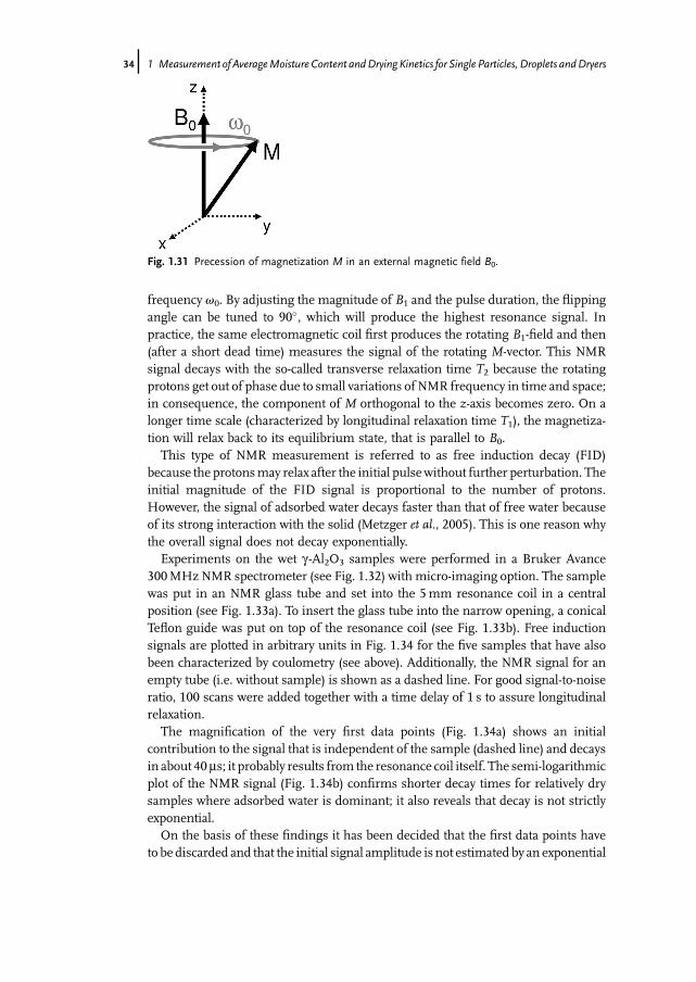
300MHz NMR spectrometer (see Fig. 1.32) with micro-imaging option. The samplewas put in an NMR glass tube and set into the 5mm resonance coil in a centralposition (see Fig. 1.33a). To insert the glass tube into the narrow opening, a conicalTeflon guide was put on top of the resonance coil (see Fig. 1.33b). Free inductionsignals are plotted in arbitrary units in Fig. 1.34 for the five samples that have alsobeen characterized by coulometry (see above). Additionally, the NMR signal for anempty tube (i.e. without sample) is shown as a dashed line. For good signal-to-noiseratio, 100 scans were added together with a time delay of 1 s to assure longitudinalrelaxation.The magnification of the very first data points (Fig. 1.34a) shows an initial

contribution to the signal that is independent of the sample (dashed line) and decaysin about 40ms; it probably results from the resonance coil itself. The semi-logarithmicplot of the NMR signal (Fig. 1.34b) confirms shorter decay times for relatively drysamples where adsorbed water is dominant; it also reveals that decay is not strictlyexponential.On the basis of these findings it has been decided that the first data points have

to be discarded and that the initial signal amplitude is not estimated by an exponential

Fig. 1.31 Precession of magnetization M in an external magnetic field B0.


fit but instead approximated by the first reasonable value (measured after 34.5ms).The reproducibility of these values was found to be around 1%.Summarizing the advantages of the described NMRmethod we may state that, in

contrast to the method of coulometry:

. No approximate knowledge is needed about the moisture content of the samplebecause the same measurement protocol is applied to wet and dry samples.

. The wet sample is not �destroyed� so the measurement may be repeated.

. Experimental time can bemade short, depending on the desired accuracy (100 s forthe chosen protocol).

. Themeasured particle moisture is affected by the gas in the test tube (about 2 cm3)only because of sampling – establishing new sorption equilibrium – and notbecause of the measurement method itself (cf. opening of oven door in coulome-try). The resulting error may be reduced by filling the empty part of the tube withinert material.

Fig. 1.32 Bruker Avance 300MHz NMR spectrometer (courtesy of Bruker Biospin Co.).


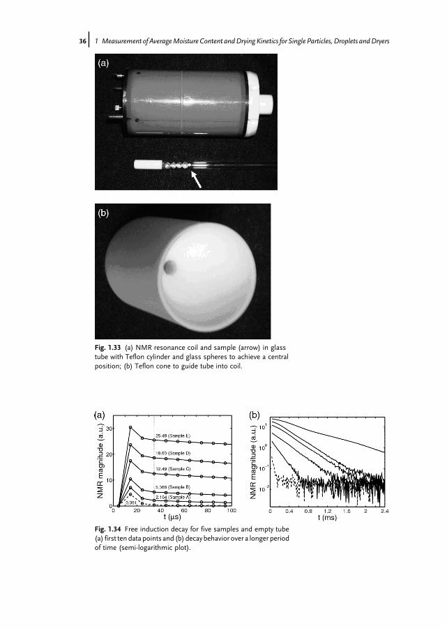
Fig. 1.33 (a) NMR resonance coil and sample (arrow) in glasstube with Teflon cylinder and glass spheres to achieve a centralposition; (b) Teflon cone to guide tube into coil.

Fig. 1.34 Free induction decay for five samples and empty tube(a) first ten data points and (b) decay behavior over a longer periodof time (semi-logarithmic plot).


The major disadvantages of the proposed NMR method are:

. The need for calibration. Ideally, the signal is proportional to themass of waterMw

so that only one point would be required. Unfortunately, we will see that strictproportionality is not observed and that a calibration curve is needed instead.

. The high cost of the system, also in terms of operation andmaintenance (especiallythe need for liquid helium and nitrogen to cool the superconducting magnet).

However, NMR devices can be found in all major research institutions because oftheir wide range of scientific applications. And the problem of calibration may besolved by combining the method with precise coulometric experiments.

1.4.6Combination of Both Methods

In Figure 1.35, the NMR signals of the five selected samples are plotted versus themass of water which has been measured (afterwards) by the method of coulometry.The non-zero signal of the empty tube is also shown. From the data points it becomesclear that one-point calibration (assuming proportionality) is not reasonable; fur-thermore, the comparison between linear andquadraticfit reveals that the correlationis not strictly linear so that a quadratic calibration curve is chosen. Several additionaldata sets (not shown here) could confirm the accuracy of the calibration curve.With this newly developed method, we will now measure distributions of particle

moisture.

1.4.7Experimental Moisture Distributions and Assessment of Model

The experiments for testing the model from Section 1.4.2 are carried out in acontinuous laboratory scale dryer as depicted in Fig. 1.21, with a diameter of 150mm

Fig. 1.35 Calibration of NMR signal by coulometry.


and a batch size of approximately 3 l. The instrumentation provides various mea-surements of temperature, pressure, pressure difference, gas flow rate, and inlet andoutlet gas moisture.Three experiments were run with different particle flow rates, but the same inlet

solids moisture content (X0¼ 0.65 kg kg�1), gas flow rate (125 kgh�1) and gas inlettemperature (80 �C).The latter corresponds toanadiabatic saturationmoisturecontentofYas¼ 22.3 g kg�1. Additional process parameters are summarized in Tab. 1.8. In themodel equations, the particle flow rate _N0 and mean residence time t�are affected.Furthermore, an increase in particle flow rate increases themoisture load of the dryer,resulting in an increase in moisture content in the gas phase. Both effects cause achange in particle moisture content distribution and need to be considered.The presented analyticalmodel contains themodel parameter p to adjust the shape

of the normalized drying curve to the respective material. As discussed in theprevious sections, the drying curve needs to be derived from experimental data. Inthis study, suchmeasurements were carried out in themagnetic suspension balance.Single particle drying was performed at a gas inlet temperature of 40 �C, a gas inletmoisture content of 0.633 g kg�1 and a pressure of 1022mbar. For these conditions,the adiabatic saturationmoisture content is 10.62 g kg�1. The gas flow rate was set to100mlmin�1, corresponding to a gas velocity of 3.6mms�1. The drying curves fortwo different runs under the same process conditions are presented in Fig. 1.36.

Tab. 1.8 Experimental and simulation parameters for particle flow rate variation.

Symbol Exp. 1 Exp. 2 Exp. 3 Unit

Mbed 0.982 0.820 0.976 kg_Mp 1.7 1.3 1 g s�1

Y 17.39 13.78 11.67 g kg�1

Xeq 0.09 0.08 0.06 kg kg�1

K 1.12· 10�3 1.96· 10�3 2.37· 10�3 s�1

Fig. 1.36 Drying curves of g-Al2O3 particles (dp¼ 1.8mm)measured in MSB at Tin¼ 40 �C, Yin¼ 0.633 g kg�1, Re¼ 0.38.


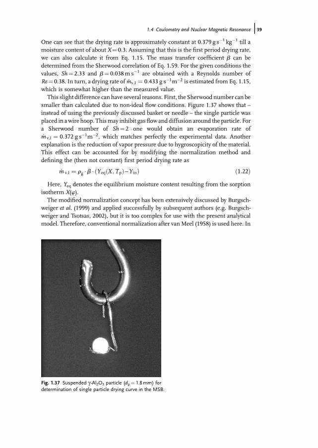
One can see that the drying rate is approximately constant at 0.379 g s�1 kg�1 till amoisture content of about X¼ 0.3. Assuming that this is the first period drying rate,we can also calculate it from Eq. 1.15. The mass transfer coefficient b can bedetermined from the Sherwood correlation of Eq. 1.59. For the given conditions thevalues, Sh¼ 2.33 and b¼ 0.038m s�1 are obtained with a Reynolds number ofRe¼ 0.38. In turn, a drying rate of _mv;I ¼ 0:433 g s�1m�2 is estimated from Eq. 1.15,which is somewhat higher than the measured value.This slight difference can have several reasons. First, the Sherwood number can be

smaller than calculated due to non-ideal flow conditions. Figure 1.37 shows that –instead of using the previously discussed basket or needle – the single particle wasplaced in awire hoop. Thismay inhibit gasflow and diffusion around the particle. Fora Sherwood number of Sh¼ 2 one would obtain an evaporation rate of_m v;I ¼ 0:372 g s�1m�2, which matches perfectly the experimental data. Anotherexplanation is the reduction of vapor pressure due to hygroscopicity of the material.This effect can be accounted for by modifying the normalization method anddefining the (then not constant) first period drying rate as

_m v;I ¼ rg �b � ðYeqðX ;TpÞ�Y inÞ ð1:22ÞHere, Yeq denotes the equilibrium moisture content resulting from the sorption

isotherm X(w).The modified normalization concept has been extensively discussed by Burgsch-

weiger et al. (1999) and applied successfully by subsequent authors (e.g. Burgsch-weiger and Tsotsas, 2002), but it is too complex for use with the present analyticalmodel. Therefore, conventional normalization after van Meel (1958) is used here. In

Fig. 1.37 Suspended g -Al2O3 particle (dp¼ 1.8mm) fordetermination of single particle drying curve in the MSB.


this frame, a critical moisture content ofXcr¼ 0.3 is read from the single particle dataof Figure 1.36 and the evaporation rate of the first drying period is determined fromEq. 1.15 with Sh¼ 2. The equilibrium moisture content Xeq is derived from thesorption isotherm provided by Groenewold et al. (2000). In this way, the normalizeddata of Fig. 1.38 are obtained for the test material.To calculate moisture distributions for the dried solids from Eq. 1.16, one needs

to fit the drying curve according to Eq. 1.14 by adjusting the parameter p. The resultof this fitting is also depicted in Fig. 1.38. For dimensionless moisture contentsF > 0.5 the fitting does not represent the experimental data very well, due to thesymmetric shape of the curve according to Eq. 1.14. This drawback is a natural priceto be paid for applying an analytical solution that does not allow for an arbitraryfunctional approximation of the normalized drying curve. Anyway, it is sufficient tojustify the method, including its experimental background, as the final results willshow.Another crucial model parameter is K. According to Eq. 1.18, K depends on the

diameter and density of the particle, the gas density and the adiabatic saturationmoisture, which can all be either measured or calculated. Furthermore, it dependson the gas-side mass transfer coefficient in the fluidized bed. For this coefficientseveral models have been suggested in the literature. In the present study we applieda Sherwood correlation recommended by Burgschweiger and Tsotsas (2002),where axial dispersion in the gas is considered in the kinetic coefficient. Finally,K depends on the moisture content in the gas bulk, Y. To predict this moisturecontent, amodel for the gas phase is required (ideal back-mixing, simple plug flow orsomemore complicatedmodel). However, and in order to keep the present approachanalytical, the parameter K was determined simply by fitting to the experimentalresults. In Tab. 1.8 the obtained values for Y and K are provided.

Fig. 1.38 Normalized drying curve for g -Al2O3 particles(dp¼ 1.8mm, Xcr¼ 0.3) and fitting by means of Eq. 1.14 withp¼ 4.


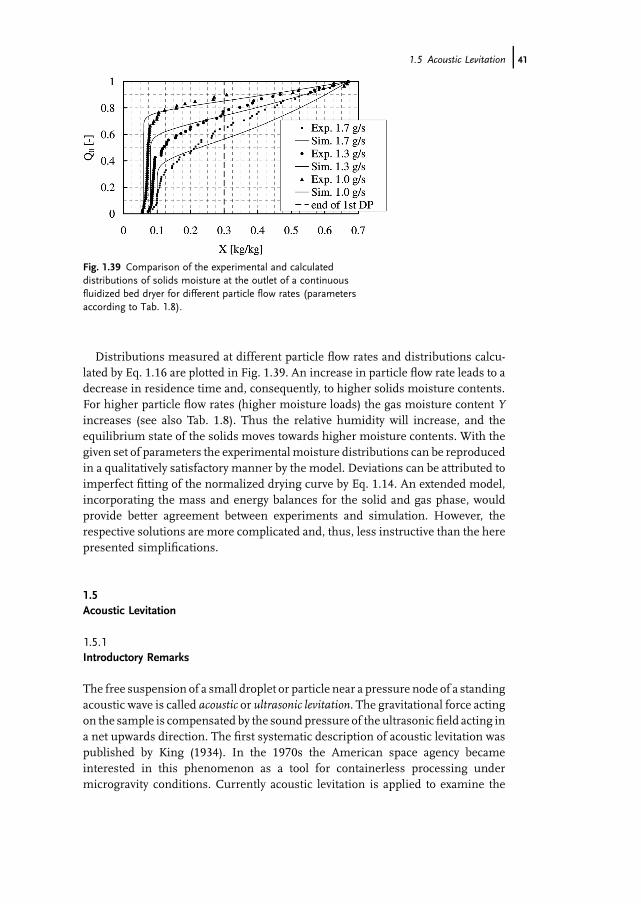
Distributions measured at different particle flow rates and distributions calcu-lated by Eq. 1.16 are plotted in Fig. 1.39. An increase in particle flow rate leads to adecrease in residence time and, consequently, to higher solids moisture contents.For higher particle flow rates (higher moisture loads) the gas moisture content Yincreases (see also Tab. 1.8). Thus the relative humidity will increase, and theequilibrium state of the solids moves towards higher moisture contents. With thegiven set of parameters the experimental moisture distributions can be reproducedin a qualitatively satisfactory manner by the model. Deviations can be attributed toimperfect fitting of the normalized drying curve by Eq. 1.14. An extended model,incorporating the mass and energy balances for the solid and gas phase, wouldprovide better agreement between experiments and simulation. However, therespective solutions are more complicated and, thus, less instructive than the herepresented simplifications.

1.5Acoustic Levitation

1.5.1Introductory Remarks

The free suspension of a small droplet or particle near a pressure node of a standingacoustic wave is called acoustic or ultrasonic levitation. The gravitational force actingon the sample is compensated by the sound pressure of the ultrasonic field acting ina net upwards direction. The first systematic description of acoustic levitation waspublished by King (1934). In the 1970s the American space agency becameinterested in this phenomenon as a tool for containerless processing undermicrogravity conditions. Currently acoustic levitation is applied to examine the

Fig. 1.39 Comparison of the experimental and calculateddistributions of solids moisture at the outlet of a continuousfluidized bed dryer for different particle flow rates (parametersaccording to Tab. 1.8).

1.5 Acoustic Levitation j41

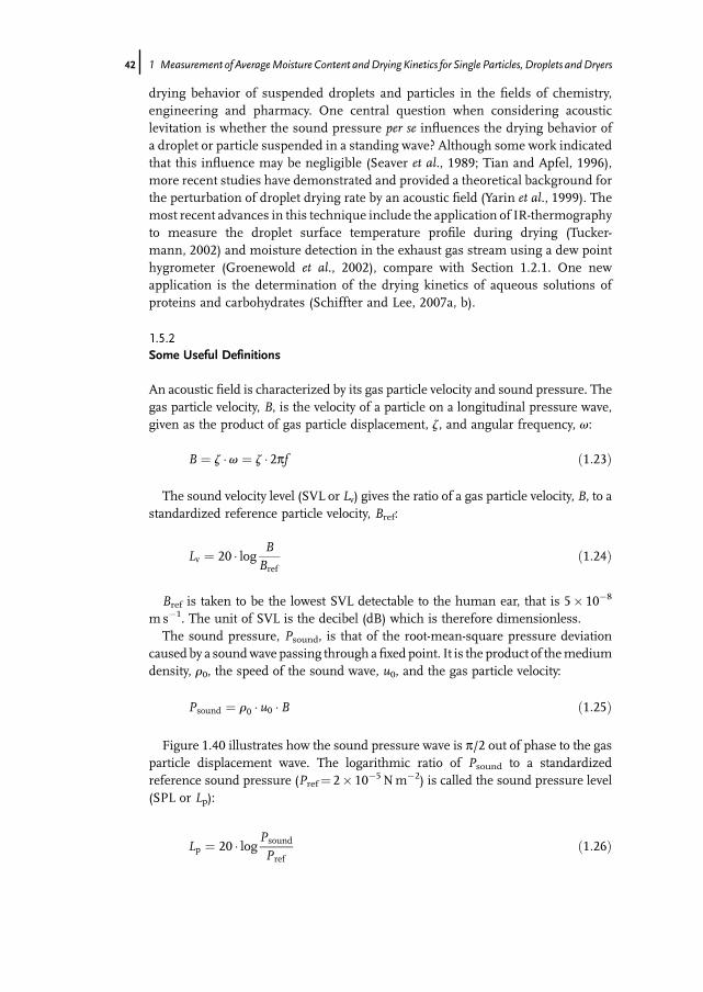
drying behavior of suspended droplets and particles in the fields of chemistry,engineering and pharmacy. One central question when considering acousticlevitation is whether the sound pressure per se influences the drying behavior ofa droplet or particle suspended in a standing wave? Although some work indicatedthat this influence may be negligible (Seaver et al., 1989; Tian and Apfel, 1996),more recent studies have demonstrated and provided a theoretical background forthe perturbation of droplet drying rate by an acoustic field (Yarin et al., 1999). Themost recent advances in this technique include the application of IR-thermographyto measure the droplet surface temperature profile during drying (Tucker-mann, 2002) and moisture detection in the exhaust gas stream using a dew pointhygrometer (Groenewold et al., 2002), compare with Section 1.2.1. One newapplication is the determination of the drying kinetics of aqueous solutions ofproteins and carbohydrates (Schiffter and Lee, 2007a, b).

1.5.2Some Useful Definitions

An acoustic field is characterized by its gas particle velocity and sound pressure. Thegas particle velocity, B, is the velocity of a particle on a longitudinal pressure wave,given as the product of gas particle displacement, z, and angular frequency, v:

B ¼ z �v ¼ z � 2pf ð1:23Þ

The sound velocity level (SVL or Lv) gives the ratio of a gas particle velocity, B, to astandardized reference particle velocity, Bref:

Lv ¼ 20 � log BBref

ð1:24Þ

Bref is taken to be the lowest SVL detectable to the human ear, that is 5� 10�8

m s�1. The unit of SVL is the decibel (dB) which is therefore dimensionless.The sound pressure, Psound, is that of the root-mean-square pressure deviation

caused by a soundwave passing through afixed point. It is the product of themediumdensity, r0, the speed of the sound wave, u0, and the gas particle velocity:

Psound ¼ r0 � u0 �B ð1:25Þ

Figure 1.40 illustrates how the sound pressure wave is p/2 out of phase to the gasparticle displacement wave. The logarithmic ratio of Psound to a standardizedreference sound pressure (Pref¼ 2� 10�5 Nm�2) is called the sound pressure level(SPL or Lp):

Lp ¼ 20 � logPsound

Prefð1:26Þ


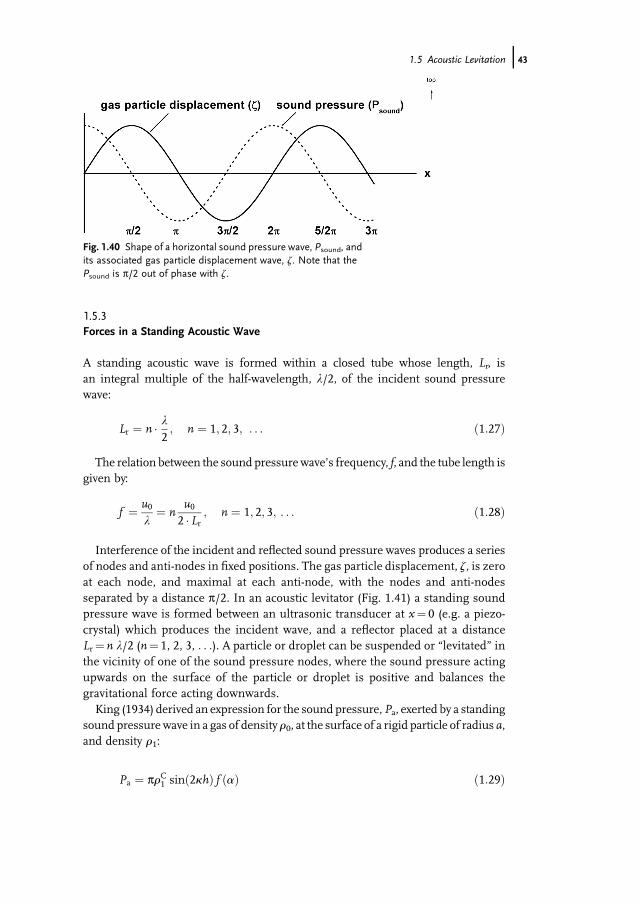
1.5.3Forces in a Standing Acoustic Wave

A standing acoustic wave is formed within a closed tube whose length, Lr, isan integral multiple of the half-wavelength, l/2, of the incident sound pressurewave:

Lr ¼ n � l2; n ¼ 1; 2; 3; . . . ð1:27Þ

The relation between the sound pressurewave�s frequency, f, and the tube length isgiven by:

f ¼ u0l

¼ nu02 � Lr ; n ¼ 1; 2; 3; . . . ð1:28Þ

Interference of the incident and reflected sound pressure waves produces a seriesof nodes and anti-nodes in fixed positions. The gas particle displacement, z, is zeroat each node, and maximal at each anti-node, with the nodes and anti-nodesseparated by a distance p/2. In an acoustic levitator (Fig. 1.41) a standing soundpressure wave is formed between an ultrasonic transducer at x¼ 0 (e.g. a piezo-crystal) which produces the incident wave, and a reflector placed at a distanceLr¼ n l/2 (n¼ 1, 2, 3, . . .). A particle or droplet can be suspended or �levitated� inthe vicinity of one of the sound pressure nodes, where the sound pressure actingupwards on the surface of the particle or droplet is positive and balances thegravitational force acting downwards.King (1934) derived an expression for the sound pressure,Pa, exerted by a standing

sound pressure wave in a gas of density r0, at the surface of a rigid particle of radius a,and density r1:

Pa ¼ prC1 sinð2khÞ f ðaÞ ð1:29Þ

Fig. 1.40 Shape of a horizontal sound pressure wave, Psound, andits associated gas particle displacement wave, z. Note that thePsound is p/2 out of phase with z.


where C0 (in ms�1) represents the constant of the solution applicable to the one-dimensional wave equation, k is the wavenumber¼v/u0, h is the displacement ofthe center of the spherical particle from a node at h¼�n�p/k, a¼ k a, and f (a) isgiven by:

f ðaÞ ¼ 1a3

F0F1 þG0G1

H20H

21

a2� 2a5

F1F2 þG1G2

H21H

22

a2�3ð1�r0=r1Þ� �

þX1n¼2

ð�1Þn nþ 1a2nþ 3

ðFnþ 1Fn þGnþ 1GnÞH2

nH2nþ 1

a2�nðnþ 2Þ� � ð1:30Þ

The coefficients Fn, Gn, and Hn are functions of a and can be expressed aspolynomials of 1/a2 (given by King, 1934) together with:

H2nðaÞ ¼ F2

nðaÞþG2nðaÞ ð1:31Þ

Equation 1.29 shows that the sound pressure acting on the particle in the standingwave is periodic and varies with the relative position of the center of the sphere to thenodes and anti-nodes. This behavior differs therefore from the sound pressure actingon a particle in a translating sound pressure wave, which is always positive.

Fig. 1.41 Representation of incident standing sound pressurewave formed between transducer and reflector in an acousticlevitator. At the pressure nodes the gas particle displacement is 0,whilst that at the empty nodes is a maximum.


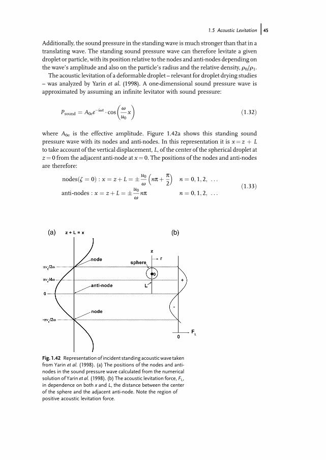
Additionally, the sound pressure in the standing wave ismuch stronger than that in atranslating wave. The standing sound pressure wave can therefore levitate a givendroplet or particle, with its position relative to the nodes and anti-nodes depending onthe wave�s amplitude and also on the particle�s radius and the relative density, r0/r1.The acoustic levitation of a deformable droplet – relevant for droplet drying studies

– was analyzed by Yarin et al. (1998). A one-dimensional sound pressure wave isapproximated by assuming an infinite levitator with sound pressure:

Psound ¼ A0ee�ivt � cos v

u0x

� �ð1:32Þ

where A0e is the effective amplitude. Figure 1.42a shows this standing soundpressure wave with its nodes and anti-nodes. In this representation it is x¼ z þ Lto take account of the vertical displacement, L, of the center of the spherical droplet atz¼ 0 from the adjacent anti-node at x¼ 0. The positions of the nodes and anti-nodesare therefore:

nodesðz ¼ 0Þ : x ¼ zþ L ¼ � u0v

npþ p2

� �n ¼ 0; 1; 2; . . .

anti--nodes : x ¼ zþ L ¼ � u0vnp n ¼ 0; 1; 2; . . .

ð1:33Þ

Fig. 1.42 Representation of incident standing acousticwave takenfrom Yarin et al. (1998). (a) The positions of the nodes and anti-nodes in the sound pressure wave calculated from the numericalsolution of Yarin et al. (1998). (b) The acoustic levitation force, FL,in dependence on both x and L, the distance between the centerof the sphere and the adjacent anti-node. Note the region ofpositive acoustic levitation force.


The effective amplitude,A0e, is selected tomake Eq. 1.32 consistent with a levitatortube length of Lr, yielding:

A0e ¼ � A0

cosðvLr=u0Þ ð1:34Þ

A0 is the amplitude at the transducer surface, that is x¼ 0. The approximatedstanding sound pressure wave described by Eqs. 1.32 and 1.34 gives node positionsthat are at most 5% removed from the exact solution for a levitator tube length of Lr(Yarin et al., 1998).This standing sound pressure wave is disturbed by the presence of a droplet

levitated in the vicinity of one of the nodes, resulting in an additional scattered soundpressure wave:

Pssound ¼ A0e � e�ivt �P�sðrÞ ð1:35Þ

where the dimensionless function P�sðrÞ of the radius vector r is found from theHelmholtz equation:

rP�s þ v

u0

� �2

P�s ¼ 0 ð1:36Þ

The total sound pressure existing at the sphere�s surface is now the sum of thesound pressures of the incident wave, Psound, plus the scattered wave, Ps

sound. Yarinet al. (1998) solved this problem by numerical evaluation of the associated boundaryintegral solutions to Eq. 1.36, and obtained the total sound pressure acting at thedroplet surface, Pa. The resulting acoustic levitation force, FL, was then obtained byintegrating Pa over the droplet from top to bottom. Their numerical result for FL independence on L could then be compared with the analytical result given for FL fromKing�s Eq. 1.29 in terms of L:

FL ¼ pr0 �a2 � A0e

r0 � u0

� �2

� sinð2a � LÞ � f ðaÞ ð1:37Þ

where f(a) is as given in Eq. 1.30. The results in Tab. 1.9 illustrate the closeness ofYarin�s approximation to King�s analytical solution in Eq. 1.37. For a sound pressurewave of intermediate length (a¼ 1) the acoustic levitation force is positive in the

Tab. 1.9 A comparison of the one-dimensional acoustic levitationforce, FL, existing along the standing sound pressure wave andacting on a sphere as calculated numerically by Yarin et al. (1998),and also from King (1934) analytical solution. FL is rendereddimensionless by dividing with r0u

20a

2, and L by dividing with a;.A0e=r0u

20 ¼ 1:0, a¼ 1.0, data taken from Yarin et al. (1998).

L FL (Yarin et al.) FL (King)

0 �0.0096 00.1 0.2737 0.2840p/4¼ 0.785 1.4148 1.42941.0 1.2849 1.2998p/2¼ 1.55 0.0466 0.0594


range of L between 0 and p/2 (Fig. 1.42a), as predicted by Eq. 1.37. Furthermore, themaximum FL exists at L¼p/4. The numerical result differs from the analytical resultby 1% (Yarin et al., 1998).Formeasurementswith an acoustic levitatorwemust knowatwhat soundpressure

level acting at the sphere�s surface, SPLeff, the device is working. SPLeff is directlyrelated to the effective amplitude of the standing sound pressure wave, A0e in dynecm�2 (Yarin et al., 1998):

SPLeff ¼ 20 � logðA0eÞþ 74 ð1:38ÞThe sound pressure level at the sound source, SPL, is related to SPLeff by using

Eq. 1.34, to yield:

SPL ¼ SPLeff þ 20 � log½�cosðv � Lr=u0Þ ð1:39ÞYarin et al. (1998) give two techniques for determiningSPLeff in a levitator. First, the

�drop-out� method that determines A0e by exploiting the balance of FL from Eq. 1.37and gravity acting on the sphere, FG¼ 4/3 pa3r1g, that exists when the sphere islevitated stably at some point between L¼ 0 and p/2. A sphere is levitated within thestanding acoustic wave at known driving voltage, U0, of the transducer. U0 is thenreduced to the pointU0m, where the sphere drops out of the wave because FL is nowtoo small to compensate FG. At this �drop-out point� the effective amplitude, A0em,can be directly calculated from the properties of the levitated sphere:

A0em ¼ 43� a � r1 � r0 � g � u

20

f ðaÞ� �1=2

ð1:40Þ

Providing the amplitude of the transducer varies linearly with U0, then A0e cannow be determined from:

A0e ¼ A0em � U0

U0mð1:41Þ

SPLeff is then directly available from Eq. 1.38 and is valid for the sphere sizeused in the experiment. The second technique calculates SPLeff from the aspect ratio(¼ horizontal radius (rh)/vertical radius (rv)) of a levitated droplet. As we shall see inSection 1.5.4.1, a droplet suspended in an acoustic field will be deformed in shape bythe asymmetric nature of the acoustic force acting on it. Yarin et al. (1998) used anumerical technique to solve the Bernoulli equation to give droplet shape as afunction of Pa. By comparing measured aspect ratio with this solution the SPLeff canbe calculated at any time during droplet drying.

1.5.4Interactions of a Droplet with the Sound Pressure Field

A levitated droplet is influenced in its behavior by the standing sound pressure wavein four ways:

1. Deformation of the droplet, owing to anisotropic axial and radial levitationforces.


2. Acoustic streaming field near the surface of the levitated droplet which leads toacoustic convection and also solvent vapor accumulation, both of which phenom-ena greatly influence droplet drying rate.

3. Heating of the droplet, owing to oscillations of the ultrasonic transducer whichchange the temperature of the ambient drying air.

4. Increasing SPLeff during evaporation as the droplet size decreases.

Any use of acoustic levitation to examine droplet or particle drying kinetics mustrecognize these effects.

1.5.4.1 Deformation of Droplet ShapeA levitated droplet may deviate from a spherical shape because the sound pressureexerted by the standing wave is not uniform over the surface of the sphere. Theextent of shape distortion depends on droplet size, the surface tension of the liquid,and the sound pressure (Trinh and Hsu, 1986; Marston et al., 1981). For example, ahigher sound pressure/SPL produces greater distortion and therefore a higheraspect ratio at fixed droplet size (Trinh and Hsu, 1986). The problem of predictinglevitated droplet shape in dependence on sound pressure, Pa, was first analyzed byMarston et al. (1981) for small deformations (Trinh and Hsu, 1986). Tian et al. (1993)extended this by including adjustment between the drop and its surroundingfield; theacoustic force that causes drop distortion is itself modified by the change in dropletshape. Yarin et al. (1998) adopted a numerical iteration technique to satisfy theequilibrium of FL and FG:

�2pðbottom

top

Paqrqs

rds ¼ 43pa3r1g ð1:42Þ

where Pa is a function of droplet shape and L. Figure 1.43 reproduces a graphicalcomparison of experimental data of aspect ratio versus Psound taken from Trinh andHsu (1986) with the predictions of Marston et al. (1981); Tian et al. (1993); Yarinet al. (1998). The deviation observed with Marston�s prediction illustrates the impor-tance of recognizing the coupling of droplet shape distortion with FL.Of particular interest is the distribution of Pa across the z-axis of the droplet

surface shown in Fig. 1.44. At the top (z� 0.5) and bottom (z��1.2) of thedroplet it is Pa > 0 and the droplet surface is compressed. In the equatorial range(�0.7 z 0.3) it is Pa < 0 and the droplet surface is stressed (Yarin et al., 1998).The result will be an oblate spheroid shape of the originally spherical droplet (Tianet al., 1993).

1.5.4.2 Primary and Secondary Acoustic StreamingThe sound pressure field around a droplet levitated in the standing wave results instreaming of the gas. The solution of the equations for an unsteady compressibleboundary layer in the gas near the droplet surface gives the velocity of this acousticstreaming, huacoustici, as the time-average of multiple cycles of the standing acoustic


wave. The velocity field is illustrated in Fig. 1.45 (Yarin et al., 1999) by the streamlinesnear the droplet surface. The distribution of huacoustici over the droplet surface isperiodic, as seen in Fig. 1.46. In this representation x is the arc length of the dropletcircumference measured from the bottom. The values of huacoustici given at x¼ 0,x¼ x2 and x¼ x3 correspond to the points O1, O2 andO3 of the droplet surface shown

Fig. 1.43 Influence of sound pressure on theaspect ratio of droplets of silicone oil levitated inan acoustic levitator (a0¼ 450mm, a¼ 0.16).The filled squares show the original experimentaldata taken from Trinh and Hsu (1986). The three

curves represent the predictions given byMarston et al. (1981); Tian et al. (1993); Yarin,Paffenlehner and Tropea (1998). This figure hasbeen redrawn from Yarin, Paffenlehner andTropea (1998).

Fig. 1.44 The distribution of sound pressure, Pa, acting on thedroplet surface along the z-axis calculated for a n-hexane dropletof a0¼ 1061mm at a transducer voltage of 156V. Note theperiodicity ofPa across the axis of the droplet surface,withPa> 0 atthe top and bottom of the droplet. In the equatorial range Pa< 0.Figure reproduced from Yarin et al. (1998).


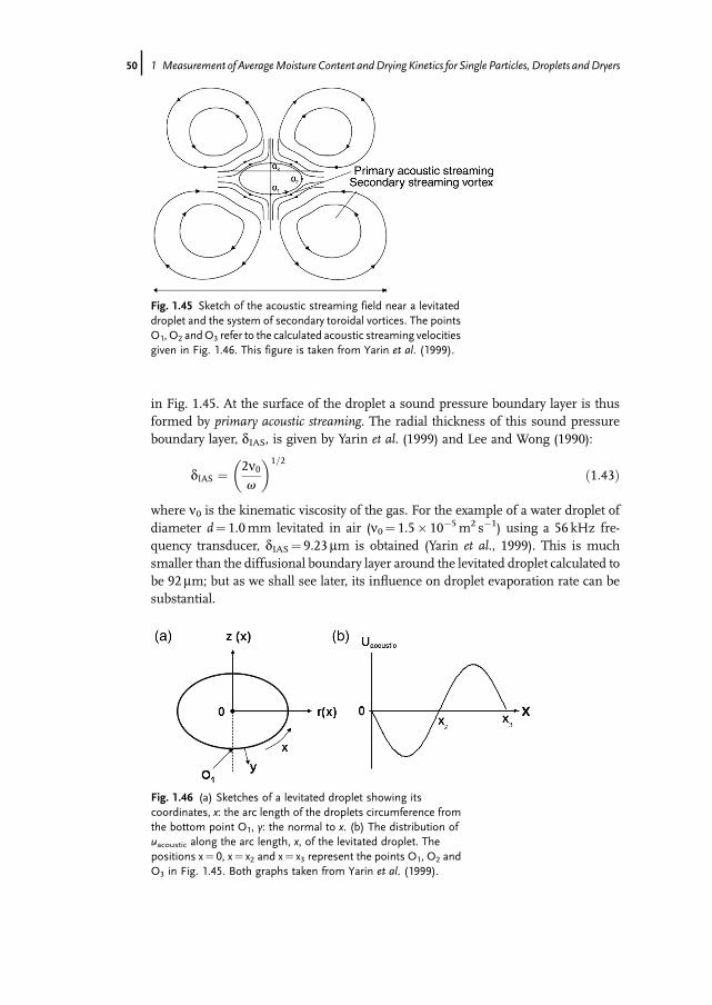
in Fig. 1.45. At the surface of the droplet a sound pressure boundary layer is thusformed by primary acoustic streaming. The radial thickness of this sound pressureboundary layer, dIAS, is given by Yarin et al. (1999) and Lee and Wong (1990):

dIAS ¼ 2n0v

� �1=2

ð1:43Þ

where n0 is the kinematic viscosity of the gas. For the example of a water droplet ofdiameter d¼ 1.0mm levitated in air (n0¼ 1.5� 10�5m2 s�1) using a 56 kHz fre-quency transducer, dIAS¼ 9.23mm is obtained (Yarin et al., 1999). This is muchsmaller than the diffusional boundary layer around the levitated droplet calculated tobe 92mm; but as we shall see later, its influence on droplet evaporation rate can besubstantial.

Fig. 1.45 Sketch of the acoustic streaming field near a levitateddroplet and the system of secondary toroidal vortices. The pointsO1, O2 andO3 refer to the calculated acoustic streaming velocitiesgiven in Fig. 1.46. This figure is taken from Yarin et al. (1999).

Fig. 1.46 (a) Sketches of a levitated droplet showing itscoordinates, x: the arc length of the droplets circumference fromthe bottom point O1, y: the normal to x. (b) The distribution ofuacoustic along the arc length, x, of the levitated droplet. Thepositions x¼ 0, x¼ x2 and x¼ x3 represent the points O1, O2 andO3 in Fig. 1.45. Both graphs taken from Yarin et al. (1999).


Primary acoustic streaming results in an enhanced convection of solvent vaporaway from the droplet surface. For a small spherical droplet wherek� 1, the solutionfor huacoustici reduces to (Yarin et al., 1999; Burdukov and Nakoryakov, 1965):

huacoustici ¼ � 4532

B2

v � a � sin 2xa

ð1:44Þ

For a water droplet levitated at an SPLeff of 165.7 dB, Eq. 1.44 predicts a velocity ofprimary acoustic streaming of up to 0.93m s�1 along the arc length of the dropletcircumference (cf. Fig. 1.46) (Yarin et al., 1999). This convectivemovement of the gasaround the dropletmust result in a Sherwoodnumber,Sh > 2.0. Yarin et al. (1999) givethe resulting distribution of the time-averaged Sh across the arc length x1 of thecircumference of a small levitated droplet as:

hShi ¼ 2454p

� �1=2 B

ðvD10Þ1=2� cos2ðx1=aÞ½1þ cos2ðx1=aÞ1=2

ð1:45Þ

The distribution of Sh is symmetrical about the vertical axis through point O3 inFig. 1.45. The average Sh over the surface of the sphere is:

hShi ¼ Kacoustic � B

ðv �D10Þ1=2ð1:46Þ

where D10 is the binary diffusivity of the solvent vapor in the gas, and Kacoustic isapproximated by:

Kacoustic ¼ 2ffiffiffip

p j h �uacoustici j �rðx�2

x�

hu�acousticir�2d x� !1=2

� v � a=u0A0e=ðr0 � u20Þ� �1=2

ð1:47Þ

The quantity r¼ a sin(x/a) is the r-coordinate of the droplet (cf. Fig. 1.46) that is setdimensionless with the initial droplet radius a0. The term uacoustic is set dimension-less with the gas particle velocity, B, and jhu�acousticij r� is averaged over the dropletsurface. As droplet shape and hence r will change continuously during evaporation,Kacoustic has to be re-calculated continuously during the drying process. The Shdeduced from Eq. 1.46 will therefore be a time-function during droplet evaporation.For a small spherical droplet a good approximation of Sh is, however, given by:

hShi ¼ 454p

� �1=2

� B

ðv �D10Þ1=2ð1:48Þ

This illustrates how, because of primary acoustic streaming, Sh depends directlyon gas particle velocity, B, and hence on SPL via Eq. 1.25. These equations do notconsider liquid flowwith the levitated droplet, which increases uacoustic by up to 10%.The corresponding increase in Sh is, however, negligible for mass transferconsiderations (Rensink, 2004).The effects of secondary acoustic streaming on droplet evaporation rate are the

opposite of that of primary acoustic streaming. Figure 1.45 illustrates that secondary


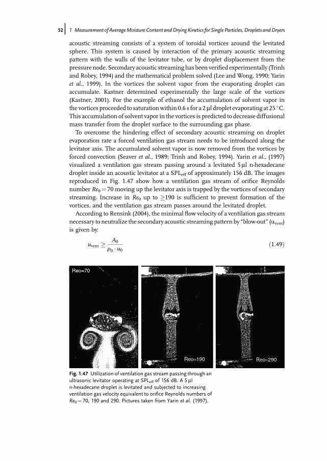
acoustic streaming consists of a system of toroidal vortices around the levitatedsphere. This system is caused by interaction of the primary acoustic streamingpattern with the walls of the levitator tube, or by droplet displacement from thepressure node. Secondary acoustic streaminghas been verified experimentally (Trinhand Robey, 1994) and the mathematical problem solved (Lee and Wong, 1990; Yarinet al., 1999). In the vortices the solvent vapor from the evaporating droplet canaccumulate. Kastner determined experimentally the large scale of the vortices(Kastner, 2001). For the example of ethanol the accumulation of solvent vapor inthe vortices proceeded to saturationwithin 0.6 s for a 2ml droplet evaporating at 25 �C.This accumulation of solvent vapor in the vortices is predicted to decrease diffusionalmass transfer from the droplet surface to the surrounding gas phase.To overcome the hindering effect of secondary acoustic streaming on droplet

evaporation rate a forced ventilation gas stream needs to be introduced along thelevitator axis. The accumulated solvent vapor is now removed from the vortices byforced convection (Seaver et al., 1989; Trinh and Robey, 1994). Yarin et al., (1997)visualized a ventilation gas stream passing around a levitated 5ml n-hexadecanedroplet inside an acoustic levitator at a SPLeff of approximately 156 dB. The imagesreproduced in Fig. 1.47 show how a ventilation gas stream of orifice Reynoldsnumber Re0¼ 70 moving up the levitator axis is trapped by the vortices of secondarystreaming. Increase in Re0 up to �190 is sufficient to prevent formation of thevortices, and the ventilation gas stream passes around the levitated droplet.According to Rensink (2004), the minimal flow velocity of a ventilation gas stream

necessary to neutralize the secondary acoustic streaming pattern by �blow-out� (uvent)is given by:

uvent � A0

r0 � u0ð1:49Þ

Fig. 1.47 Utilization of ventilation gas stream passing through anultrasonic levitator operating at SPLeff of 156 dB. A 5mln-hexadecane droplet is levitated and subjected to increasingventilation gas velocity equivalent to orifice Reynolds numbers ofRe0¼ 70, 190 and 290. Pictures taken from Yarin et al. (1997).


Recall thatA0 is the amplitude of the sound pressure wave at the transducer sourcesurface (Eq. 1.34). For a water droplet levitated at a SPL of 165.7 dB the predicted uventis 4.3m s�1. A ventilation gas velocity lower than uvent can, however, be sufficient toprevent accumulation of solvent vapor in the toroidal vortices. This was shown to betrue experimentally by Rensink (2004) for different solvent droplets.

1.5.4.3 Effects of Changing Droplet SizeAs elucidated in Section 1.5.4.1, a droplet levitated in a standing sound pressurewaveis deformed to an oblate spheroid because the sound pressure acting on the droplet isnot uniform along the sphere surface. During evaporation both the shape and theposition of the droplet will, however, change. The droplet shape converges to that of asphere (Kastner, 2001). The total pressure difference across the droplet surfacecomprises three parts (Tian et al., 1993):

Pi�Po ¼ DPs þDPG þDPst ð1:50Þ

where Pi and Po are the pressures at the surface approached from the inside oroutside, respectively; DPs is the contribution from the sound pressure wave, DPG isinduced by gravity, and DPst is the difference in uniform static pressure inside andoutside the droplet. In the absence of a sound pressure wave

DPst ¼ 2s=a ð1:51Þ

where s is the surface tension of the liquid. Now, as the droplet shrinks duringevaporation the decreasing radius of curvature will make DPst dominant over DPrad(Trinh and Hsu, 1986). The aspect ratio will therefore approach unity as thecontribution from DPrad in Eq. 1.50 becomes less. Figure 1.48 shows experimental

Fig. 1.48 Influence of shrinking droplet size on aspect ratio duringevaporation; k¼v/u0, a: droplet radius). Data taken from Trinhand Hsu (1986).


data for evaporating water droplets. The decrease in k a at fixed SPL causes the aspectratio to decrease and approach unity.Simultaneously the displacement of the droplet center from the nearest pressure

node, Dz, decreases because the evaporating droplet rises in the standing soundpressure wave within the range 0 < L< 2p (Yarin et al., 1999). This is caused by adecreasing resonance shift of the levitator as droplet size decreases.When the dropletis introduced into the standing sound pressure wave it will immediately be deformedinto an oblate spheroid (see Section 1.5.4.1). This change in droplet shape alters thescattered sound pressure wave, shifts hereby the resonance of the levitator, anddecreases the sound pressure acting on the droplet surface,Pa (Trinh andHsu, 1986).During evaporation the droplet size decreases and hence the resonance shift inducedby the droplet will be progressively ameliorated. The result is a continual increase inSPLeff, which returns to its unperturbed value when the droplet has disappeared.Figure 1.49 shows how the SPLeff increases with decreasing droplet size duringevaporation (Yarin et al., 1998). The SPL needed to levitate the drop is directlyproportional to the liquid�s density, r1. An increase in SPLeff means, however, ahigher gas particle velocity,B, and hence increased Sh in Eq. 1.46. This occurs duringdroplet evaporation in a sound pressurefield and is expected to influence evaporationrate.The decrease in droplet size during drying and the resulting increase in SPLeff will

raise FL and cause a rise of the levitated droplet in the standingwave. Furthermore, asthe mass of the levitated droplet decreases, the balance of gravitational and levitationforces, FG and FL, dictates that the droplet rises in the standing wave:

43p � a3 � r1 � g ¼ pr0 � a2 �

A0e

r0 � u0

� �2

� sinð2a � LÞ � f ðaÞ ð1:52Þ

Fig. 1.49 Increase in SPLeff as droplet volume decreases duringevaporation for four solvents. The SPLeff was calculated fromthe change in the aspect ratio of the droplets during drying.Fig. taken from Yarin et al. (1998).


As droplet mass (4/3 pa3r1) decreases because of solvent evaporation, the sinefunction must decrease proportionately and the droplet rises within the soundpressure wave. Figure 1.50 taken from Kastner (2001) illustrates the influence ofloss of mass on Dz of a droplet according to Eq. 1.52. A decrease in droplet volume atconstant droplet density has a much weaker effect on Dz than does a decrease indensity at constant volume.In terms of drying of a solution droplet, the change in Dz is caused by progressive

resonance amelioration and by decreasing droplet size till a solid porous particle hasemerged (critical point). The subsequent change in Dz of the particle after the criticalpoint is caused by change in density during solvent loss, since particle size nowremains constant. This can be exploited to determine particle drying kinetics after thecritical point (Yarin et al., 1999; Kastner et al., 2001).

1.5.5Single Droplet Drying in an Acoustic Levitator

1.5.5.1 Drying Rate of a Spherical Solvent DropletMass transfer from an evaporating droplet suspended in a gas phase was alsodiscussed in Chapter 5, Vol. 1 of this series, in the context of spray dryer simulation.In general, two approaches can be applied. The first is to solve the conservationequations for a motionless sphere in an infinite stagnant medium, and to employ anempirical correction factor to account for forced convection around the droplet(Frohn andRoth, 2000). The second is to usefilm theory with analysis of the effects offorced convection on layer thicknesses for heat and mass transfer (Sirignano, 2000).

Fig. 1.50 Position of droplet within sound pressure wave isdependence on its mass. Dz is the distance between the centerof mass of the droplet and the adjacent pressure node. Theupper line shows how Dz changes with decreasing volume atconstant density. The lower line shows the behavior as densitydecreases at constant volume. These data were taken fromKastner (2001).


The first approach leads to the d2-law and is a steady-state, gas phase model atconstant temperature. A single, spherical droplet of initial radius a0 and fixed surfacetemperature, Tph, is suspended in a still gas phase of fixed temperature T1. At thedroplet surface the saturation vapor pressure of the liquid, p�, exists, whilst in the gasphase there is a lower vapor pressure, p1. Solution of the one-dimensional diffusionequation for vapor flow rate at the droplet surface, _Mv, yields (Frohn and Roth, 2000):

_Mv ¼ 4p �D10 � aðtÞfp��p1g � ~M=ð~RTÞ ð1:53Þ

whereD10 is the diffusivity of the vapor in the gas phase, ~M is liquidmolecularmass,and ~R is the universal gas constant. The rate of shrinkage of the sphere, _Mdrop, is givenby:

_Mdrop ¼ 4p � r1 � a2ðtÞ �dadt

ð1:54Þ

Conservation of mass at the receding droplet surface specifies that:

_Mv ¼ _Mdrop ð1:55Þto yield for the time-profile of a(t), otherwise known as the d2-law:

a2ðtÞ ¼ a20 �b � t ð1:56Þ

b ¼ 2D10 ~M

r1~R

p�

Tph� p1T1

�ð1:57Þ

Droplet lifetime, tl, is then given by:

tl ¼r1a0~RðTph�T1Þ2D10 ~MðPph�p1Þ ð1:58Þ

The d2-law is valid in still gas, but can be corrected in an empirical fashion toaccount for forced convection of the gas phase. A good approximation is that of Ranzand Marshall (1952) determined for a suspended solvent drop:

Nu ¼ 2þ 0:6 �Re1=2 �Pr1=3Sh ¼ 2þ 0:6 �Re1=2 �Pr1=3

ð1:59Þ

To describe the evaporation rate under forced convection conditions around a puresolvent droplet Eq. 1.57 is therefore changed to (Tuckermann et al., 2002):

b ¼ 2D10 ~M

r1~R

p�

Tph� p1T1

�� Sh2

ð1:60Þ

The above equations do not account for any influences of the sound pressure fieldon gas movement around a levitated droplet, that is, acoustic streaming.


The alternative approach to droplet drying kinetics according to Sirignano (2000) isbased on film theory to determine the radii, r, of the heat (index: t) andmass transfer(index: m) films around an evaporating sphere in a moving gas phase (forcedconvection):

rfilm;t ¼ a � Nu�

Nu��2

rfilm;m ¼ a � Sh�

Sh��2

ð1:61Þ

Nu� and Sh� are themodified Nusselt and Sherwood numbers that account for thefilm thinning effects of Stefan flow:

Nu� ¼ 2þ Nu�2Ft

Sh� ¼ 2þ Sh�2Fm

ð1:62Þ

The correction factors Ft and Fm are functions of the film thicknesses for heat andmass transfer, dt and dm:

Ft ¼ dtdt;0

Fm ¼ dmdm;0

ð1:63Þ

dt,0 and dm,0 are the initial film thicknesses at t¼ 0. The result of Abramzon andSirignano (1989) for the time-profile of a(t) is analogous to Eq. 1.60:

a2ðtÞ ¼ a20ðtÞ�bfilm � t ð1:64Þ

bfilm ¼ 2 � r0 �D10

r1� lnð1�BMÞ � Sh

�

2ð1:65Þ

Here

BM ¼ yph�y11�yph

ð1:66Þ

is the Spalding transfer number that represents the driving force for vapor diffusionthrough a stagnantfilm (Frohn andRoth, 2000). y is themass fraction of solvent vaporin the gas. For a spherical droplet in an environment with no forced convection it isSh¼ 2.0, and Eq. 1.66 simplifies to:

bfilm ¼ 2 � r0 �D10

r1� lnð1�BMÞ ð1:67Þ

which is directly analogous to the d2-law. Again, these equations take no account ofthe influence of sound pressure field on evaporation rate.


1.5.5.2 Drying Rate of an Acoustically Levitated Solvent DropletThe problem of determining the effect of a sound pressure wave on the evaporationrate of a levitated droplet was tackled by Yarin et al. (1999). For a small sphere theaverage Sh over the sphere surface is a function of gas particle velocity, B, as given byEq. 1.48. Since Sh is defined as

hShi ¼ k2a �D10

ð1:68Þ

where k is the time-averagedmass transfer coefficient at the droplet surface, it followsthat

k ¼ 12

454p

� �1=2 B

ðvD10Þ1=2� D10

að1:69Þ

The vapor flow rate at the droplet surface, _Mv, is therefore:

_Mv ¼ 4pka2ðcph�c1Þ

¼ 2pa454p

� �1=2

BD10

v

� �1=2

ðcph�c1Þ

ð1:70Þ

where c is the mass concentration of solvent vapor in the gas. Conservation of masson equating Eq. 1.70 with the rate of shrinkage of the sphere, _Mdrop in Eq. 1.54, gives:

a2ðtÞ ¼ a20�bacoustic � t ð1:71Þ

bacoustic ¼454p

� �1=2

BD10

v

� �1=2 cph�c1r1

ð1:72Þ

Since ðcph�c1Þ ¼ ~Mðp��p1Þ=ð~RTÞ for an ideal gas:

bacoustic ¼454p

� �1=2B ~M

r1~R

D10

v

� �1=2 p�

Tph� p1T1

�ð1:73Þ

Equations 1.71 and 1.73 are analogous to the d2-law Eqs. 1.56 and 1.57 with theinfluence of primary acoustic streaming, uacoustic, being accounted for. The dropletlifetime, tl, is given in this case by:

tl ¼r1a

20~RðTph�T1Þ

f45D10=ð4pvÞg1=2B ~Mðp��p1Þð1:74Þ

which is shorter than that predicted by the d2-law by the factor given byEq. 1.48 forSh.

1.5.5.3 Drying Rate of Droplets of Solutions or SuspensionsThe first drying period of a droplet of a solution or suspension resembles that of apure solvent droplet. It can therefore be described by the same equations, but takinginto account the lowering of the vapor pressure by the dissolved substance. The


temporal decrease in droplet volume, DV, gives directly the evaporation rate duringthis �constant-rate� drying period (Kastner, 2001):

_Mcr ¼ �r1 �DVDt

ð1:75Þ

Ignoring the effect of the dissolved substance, a2ðtÞ=a20 decreases linearlywith timeaccording to either Eq. 1.56 (d2-law), Eq. 1.64 byAbramzon and Sirignano or Eq. 1.71.After the critical point has been reached, the volume of the particle now existingshould remain constant (Sherwood, 1929). Continued evaporation of solvent fromthe particle decreases both itsmass and its density. As discussed in Section 1.5.4, thiswill cause the particle to rise (Dz decreases) within the ultrasonic field tomaintain thebalance between FL and FG given by Eq. 1.52 at constant SPLeff. This particlemovement can be used to determine the quantity of solvent evaporated in the seconddrying period, provided the SPLeff and hence A0e does not change after the criticalpoint, and is known. The evaporation rate in this �falling-rate� drying period is thengiven directly from Eq. 1.37 (Yarin et al., 1999; Kastner et al., 2001):

_Mfr ¼ pr0a2

Dt gA0e

r0 � u0

� �2f ðaÞ sinð2aL1Þ�sinð2aL2Þf g ð1:76Þ

determined from the droplet position at two times, L1 and L2, separated by Dt. Once_Mfr is known, the mean particle density, rp, the mean moisture mass fraction of thedroplet, x1, and the mean particle porosity, e, can be calculated as time-functions(Kastner et al., 2001):

rpðtÞ ¼MlðtÞþMs

Vp

x1ðtÞ ¼ MlðtÞMlðtÞþMs

eðtÞ ¼ 1� Ms

rs �Vp

ð1:77Þ

Ultrasonic levitation is therefore one of the few techniques suitable for examin-ing the drying process of a solution droplet during both drying periods. Theevaporation rate ( _Mcr or _Mfr) and residual solvent mass fraction (x1) of a droplet/particle can be determined at any desired point of time during evaporation.Furthermore, a droplet or particle can be removed from the levitation tube at anytime for further analysis.

1.5.6A Case Study: Single Droplet Drying of Water and an Aqueous Carbohydrate Solution

Recent studies of the drying behavior of levitated single droplets include puresolvents (Tuckermann et al., 2002), inorganic colloidal solids (Kastner et al., 2001),enzymes (Weis and Nardozzi, 2005), and surfactants (Frost et al., 1994). A study of


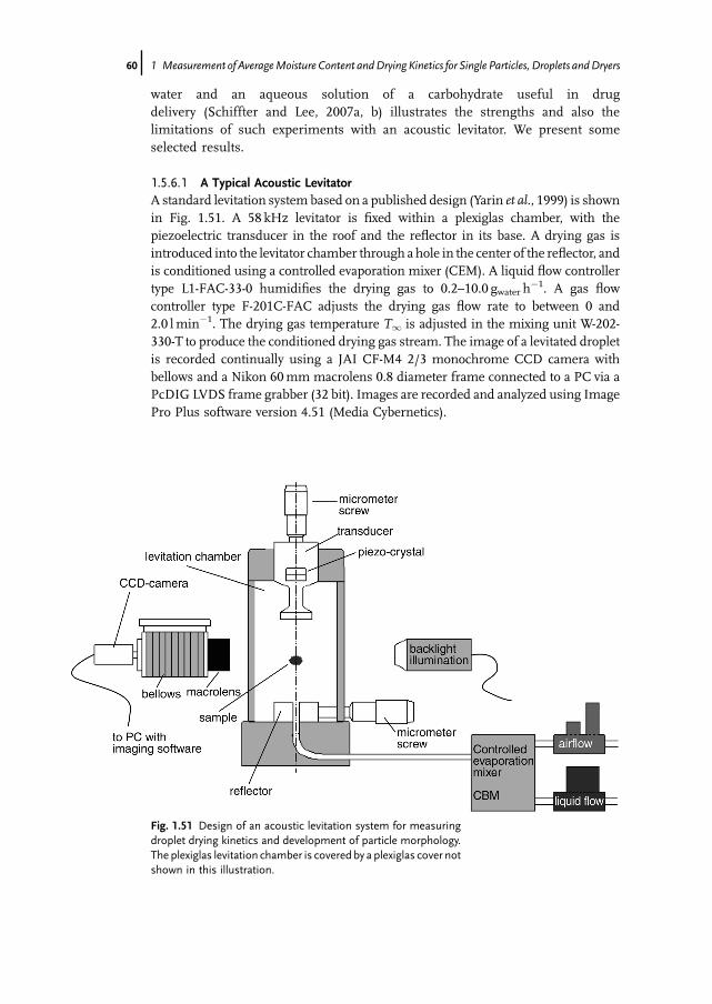
water and an aqueous solution of a carbohydrate useful in drugdelivery (Schiffter and Lee, 2007a, b) illustrates the strengths and also thelimitations of such experiments with an acoustic levitator. We present someselected results.

1.5.6.1 A Typical Acoustic LevitatorA standard levitation system based on a published design (Yarin et al., 1999) is shownin Fig. 1.51. A 58 kHz levitator is fixed within a plexiglas chamber, with thepiezoelectric transducer in the roof and the reflector in its base. A drying gas isintroduced into the levitator chamber through a hole in the center of the reflector, andis conditioned using a controlled evaporation mixer (CEM). A liquid flow controllertype L1-FAC-33-0 humidifies the drying gas to 0.2–10.0 gwater h

�1. A gas flowcontroller type F-201C-FAC adjusts the drying gas flow rate to between 0 and2.0 lmin�1. The drying gas temperature T1 is adjusted in the mixing unit W-202-330-T to produce the conditioned drying gas stream. The image of a levitated dropletis recorded continually using a JAI CF-M4 2/3 monochrome CCD camera withbellows and a Nikon 60mm macrolens 0.8 diameter frame connected to a PC via aPcDIG LVDS frame grabber (32 bit). Images are recorded and analyzed using ImagePro Plus software version 4.51 (Media Cybernetics).

Fig. 1.51 Design of an acoustic levitation system for measuringdroplet drying kinetics and development of particle morphology.The plexiglas levitation chamber is covered by a plexiglas cover notshown in this illustration.


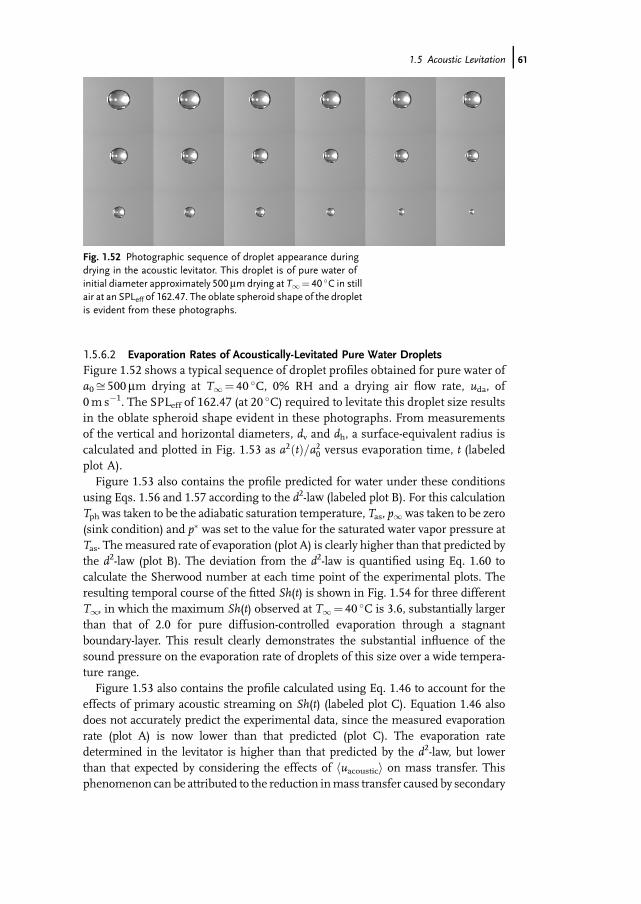
1.5.6.2 Evaporation Rates of Acoustically-Levitated Pure Water DropletsFigure 1.52 shows a typical sequence of droplet profiles obtained for pure water ofa0ffi 500 mm drying at T1¼ 40 �C, 0% RH and a drying air flow rate, uda, of0m s�1. The SPLeff of 162.47 (at 20 �C) required to levitate this droplet size resultsin the oblate spheroid shape evident in these photographs. From measurementsof the vertical and horizontal diameters, dv and dh, a surface-equivalent radius iscalculated and plotted in Fig. 1.53 as a2ðtÞ=a20 versus evaporation time, t (labeledplot A).Figure 1.53 also contains the profile predicted for water under these conditions

using Eqs. 1.56 and 1.57 according to the d2-law (labeled plot B). For this calculationTph was taken to be the adiabatic saturation temperature, Tas, p1was taken to be zero(sink condition) and p� was set to the value for the saturated water vapor pressure atTas. Themeasured rate of evaporation (plot A) is clearly higher than that predicted bythe d2-law (plot B). The deviation from the d2-law is quantified using Eq. 1.60 tocalculate the Sherwood number at each time point of the experimental plots. Theresulting temporal course of the fitted Sh(t) is shown in Fig. 1.54 for three differentT1, in which the maximum Sh(t) observed at T1¼ 40 �C is 3.6, substantially largerthan that of 2.0 for pure diffusion-controlled evaporation through a stagnantboundary-layer. This result clearly demonstrates the substantial influence of thesound pressure on the evaporation rate of droplets of this size over a wide tempera-ture range.Figure 1.53 also contains the profile calculated using Eq. 1.46 to account for the

effects of primary acoustic streaming on Sh(t) (labeled plot C). Equation 1.46 alsodoes not accurately predict the experimental data, since the measured evaporationrate (plot A) is now lower than that predicted (plot C). The evaporation ratedetermined in the levitator is higher than that predicted by the d2-law, but lowerthan that expected by considering the effects of huacoustici on mass transfer. Thisphenomenon can be attributed to the reduction inmass transfer caused by secondary

Fig. 1.52 Photographic sequence of droplet appearance duringdrying in the acoustic levitator. This droplet is of pure water ofinitial diameter approximately 500mmdrying at T1¼ 40 �C in stillair at an SPLeff of 162.47. The oblate spheroid shape of the dropletis evident from these photographs.


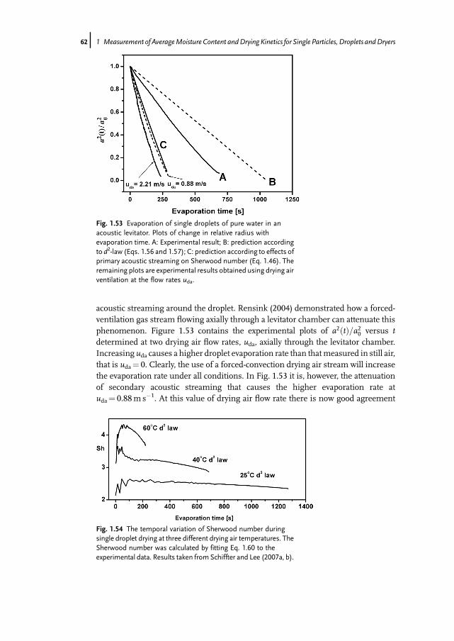
acoustic streaming around the droplet. Rensink (2004) demonstrated how a forced-ventilation gas stream flowing axially through a levitator chamber can attenuate thisphenomenon. Figure 1.53 contains the experimental plots of a2ðtÞ=a20 versus tdetermined at two drying air flow rates, uda, axially through the levitator chamber.Increasing uda causes a higher droplet evaporation rate than thatmeasured in still air,that is uda¼ 0. Clearly, the use of a forced-convection drying air stream will increasethe evaporation rate under all conditions. In Fig. 1.53 it is, however, the attenuationof secondary acoustic streaming that causes the higher evaporation rate atuda¼ 0.88m s�1. At this value of drying air flow rate there is now good agreement

Fig. 1.53 Evaporation of single droplets of pure water in anacoustic levitator. Plots of change in relative radius withevaporation time. A: Experimental result; B: prediction accordingto d2-law (Eqs. 1.56 and 1.57); C: prediction according to effects ofprimary acoustic streaming on Sherwood number (Eq. 1.46). Theremaining plots are experimental results obtained using drying airventilation at the flow rates uda.

Fig. 1.54 The temporal variation of Sherwood number duringsingle droplet drying at three different drying air temperatures. TheSherwood number was calculated by fitting Eq. 1.60 to theexperimental data. Results taken fromSchiffter and Lee (2007a, b).


between the experimental plot and that predicted fromEq. 1.46 (plot C). According toRensink (2004) this drying air flow rate prevents the accumulation of water vapor inthe levitator tube by destroying the vortices and hence neutralizes the retarding effectof secondary acoustic streaming on the droplet evaporation rate.Ifuda is higher than that necessary to neutralize secondary acoustic steaming, then a

further increase in evaporation rate is observed (Fig. 1.53 for the example uda¼ 2.21ms�1). This additional, convection-driven evaporation can most conveniently beanalyzed using Ranz and Marshall�s correlation between Sh and uda (Eq. 1.59).Figure 1.55 illustrates the example of uda¼ 1.77ms�1 at T1¼ 40 �C and uda¼ 1.7m�1 s at 25 �C. Reasonable agreement is obtained between the measured profiles ofSh(t) calculated by fitting Eq. 1.60 to the a(t)-profile and that predicted by Eq. 1.59.The experimental results are, however, only predicted accurately by Ranz-Marshallwhen uda is higher than that value found necessary to neutralize secondary acousticstreaming. With lower values of udaEq. 1.59 is inaccurate, because the drying airstream in this flow range contributes to neutralizing an accumulation of solvent vaporwithin the vortices.

1.5.6.3 Evaporation Rates and Particle Formation with Aqueous MannitolSolution DropletsThe sequence of photographs in Fig. 1.56 shows the drying of a single droplet of a10wt% aqueous solution of mannitol. The position of the critical point and subse-quent particle formation can be seen. Figure 1.57 shows a2ðtÞ=a20 versus t for thissystem dried at T1¼ 60 �Cand 0%RH in still air. The plot is initially slightly concaveto the x-axis up to a clear break at the critical point of drying tcp. The droplet�s aspectratio decreases linearly up to the critical point, as DPst becomes more dominant in

Fig. 1.55 Measured andpredicted values of Sherwoodnumber forsingle droplet drying of pure water under conditions of drying airforced convection. The irregular plots are results obtained byfitting Eq. 1.60 to the experimentally determined values of dropletradius versus evaporation time. The straight lines are thosepredicted by Ranz and Marshall�s correlation (Eq. 1.59). Datataken from Schiffter and Lee (2007a, b).


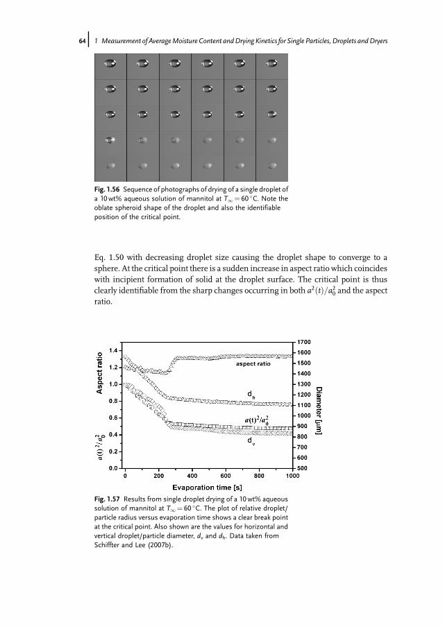
Eq. 1.50 with decreasing droplet size causing the droplet shape to converge to asphere. At the critical point there is a sudden increase in aspect ratio which coincideswith incipient formation of solid at the droplet surface. The critical point is thusclearly identifiable from the sharp changes occurring in both a2ðtÞ=a20 and the aspectratio.

Fig. 1.56 Sequence of photographs of drying of a single droplet ofa 10wt% aqueous solution of mannitol at T1¼ 60 �C. Note theoblate spheroid shape of the droplet and also the identifiableposition of the critical point.

Fig. 1.57 Results from single droplet drying of a 10wt% aqueoussolution of mannitol at T1¼ 60 �C. The plot of relative droplet/particle radius versus evaporation time shows a clear break pointat the critical point. Also shown are the values for horizontal andvertical droplet/particle diameter, dv and dh. Data taken fromSchiffter and Lee (2007b).


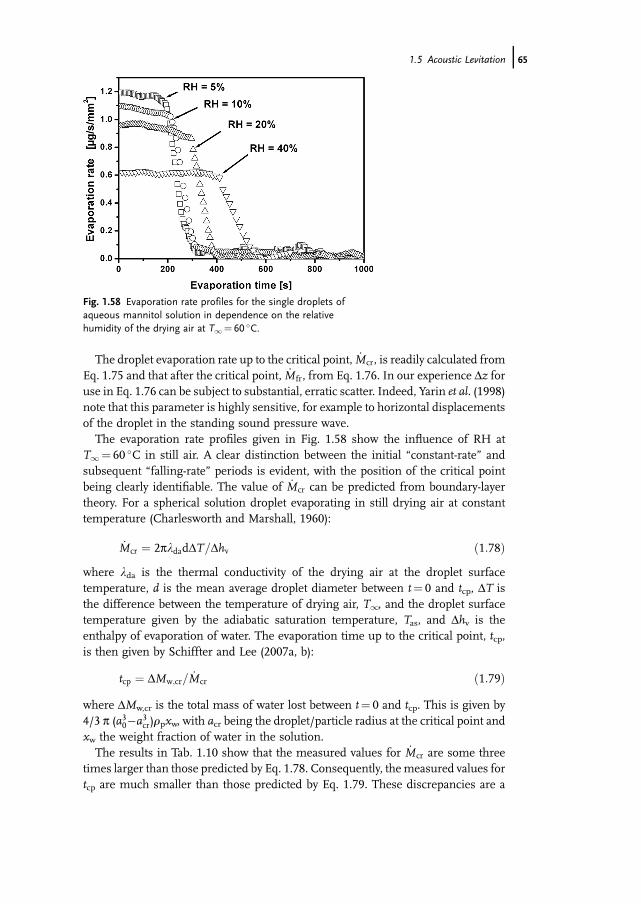
The droplet evaporation rate up to the critical point, _Mcr, is readily calculated fromEq. 1.75 and that after the critical point, _Mfr, from Eq. 1.76. In our experience Dz foruse in Eq. 1.76 can be subject to substantial, erratic scatter. Indeed, Yarin et al. (1998)note that this parameter is highly sensitive, for example to horizontal displacementsof the droplet in the standing sound pressure wave.The evaporation rate profiles given in Fig. 1.58 show the influence of RH at

T1¼ 60 �C in still air. A clear distinction between the initial �constant-rate� andsubsequent �falling-rate� periods is evident, with the position of the critical pointbeing clearly identifiable. The value of _Mcr can be predicted from boundary-layertheory. For a spherical solution droplet evaporating in still drying air at constanttemperature (Charlesworth and Marshall, 1960):

_Mcr ¼ 2pldadDT=Dhv ð1:78Þwhere lda is the thermal conductivity of the drying air at the droplet surfacetemperature, d is the mean average droplet diameter between t¼ 0 and tcp, DT isthe difference between the temperature of drying air, T1, and the droplet surfacetemperature given by the adiabatic saturation temperature, Tas, and Dhv is theenthalpy of evaporation of water. The evaporation time up to the critical point, tcp,is then given by Schiffter and Lee (2007a, b):

tcp ¼ DMw;cr= _Mcr ð1:79Þwhere DMw,cr is the total mass of water lost between t¼ 0 and tcp. This is given by4/3 p (a30�a3cr)rpxw, with acr being the droplet/particle radius at the critical point andxw the weight fraction of water in the solution.The results in Tab. 1.10 show that the measured values for _Mcr are some three

times larger than those predicted by Eq. 1.78. Consequently, themeasured values fortcp are much smaller than those predicted by Eq. 1.79. These discrepancies are a

Fig. 1.58 Evaporation rate profiles for the single droplets ofaqueous mannitol solution in dependence on the relativehumidity of the drying air at T1¼ 60 �C.


consequence of the effect of huacoustici around the levitated droplet, as we have alreadyseen in Section 1.5.6.2 with pure water. It is likely that these discrepancies betweenmeasured andpredicted evaporation rateswill depend on the initial SPLeff required tolevitate a particular droplet size. Tian and Apfel (1996) found, for example, noinfluence of a sound pressure field of low SPL of <150 dB on droplet evaporation rateand obtained a good agreement with Eqs. 1.56 and 1.57.Lower _Mcr results in a decrease in the quotient of the dried particle to initial

droplet radii, ap/a0 (Tab. 1.10), at the same solids content. Since a(t) changes onlymarginally after the critical point, the value of ap/a0 represents that size at which theprecipitatingmannitol forms amechanically-stable crust at the droplet surface. Thetime to this point is shifted to longer valueswhen _Mcr is reduced. If the droplet driesto a solid particle then ap=a0 ¼ ffiffiffiffiffiffiffiffiffiffiffi

rm;0=rs3p

, where rs is the true density of the solid. Asolid, fully-crystalline particle would fully dry to ap/a0¼ 0.405. The measuredvalues in Tab. 1.10 are all substantially higher than this theoretical result and give aquantitative measure of degree of particle porosity or hollowness. The dryingbehavior of the mannitol solution droplets is thus characterized by a sharp criticalpoint caused by crystallization from a super-saturated surface solution, followed bya rapid decline in evaporation rate as moisture must now penetrate through thepermeable crystalline crust.

1.6Concluding Remarks

The present chapter has presented experimental techniques such as:

. gravimetry by magnetic suspension balance

. dew point mirror hygrometry

. infrared spectroscopy

. nuclear magnetic resonance

. coulometry

. acoustic levitation.

Tab. 1.10 Single droplet drying kinetics of aqueous mannitol10wt% (rm,0¼ 100 kgm�3) solution at drying air temperatureT1¼ 60 �C in still air (uda¼ 0). Symbols: RH¼ relative humidityof drying air; _Mcr ¼ drying rate before critical point; tcp¼ time tocritical point; ap¼ dry particle radius; a0¼ initial droplet radius.Data taken from Schiffter and Lee (2007b).

RH[%]

Measured M_ cr[kg h�1] · 10�6

Predicted M_ cr[kg h�1] · 10�6

Measured tcp[s]

Predicted tcp[s] ap/a0

5 29.3 8.95 202 503 0.5910 26.5 8.33 234 554 0.5720 23.5 7.22 332 669 0.5340 15.2 5.27 453 950 0.49


With the help of examples, we have shown how these techniques can be used to:

. measure single particle drying kinetics

. determine kinetics of single drying droplets

. measure the distribution of moisture in a population of particles

. monitor the change of solids moisture content in convective dryers

. derive drying curves for the entire hold-up of dryers that can be scaled-down tosingle particle kinetics if an appropriate model is available.

What the discussed experimental techniques do not provide is resolution of thespatial distribution of moisture in drying solids. Methods capable of delivering thisinformation are the subject of Chapters 2–4.

Additional Notation Used in Chapter 1

A amplitude of pressure standing wave kgm�1 s�2

a droplet radius mB gas particle velocity m s�1

B magnetic field strength TBM Spalding transfer number —

c mass concentration of vapor kgm�3

F force kgm s�2

F correction factor, function —

f frequency s�1

h displacement m or dimensionlessK drying rate constant s�1

L vertical displacement mLp sound pressure level (SPL) —

Lr tube length mLv sound velocity level (SVL) —

M magnetization T_N particle flow rate s�1

p shape parameter of drying curve —

Q normalized cumulative number density —

Q electric charge CT relaxation time sU voltage V

Greek letters

a wavenumber times particle radius —

b droplet evaporation constant s�1

d boundary layer thickness mz gas particle displacement mk wavenumber m�1

Additional Notation Used in Chapter 1 j67

l wavelength mt residence time so angular frequency s�1

Subscripts and superscripts

a acousticBL balance display without sampleBLS balance display with samplecp (or: cr) critical pointcr (or: I) constant rateda drying aire (or: eff) effectivefr falling rateG gravityh horizontalIAS acoustic boundary layerL load cage and basketL levitationm drop-outm mass transferS samples scatteredst statict heat transferv verticalvent ventilation0 initial, inlet, driving0 (or: g) surrounding medium, gashi time-average over cycles� spatial average over droplet

Abbreviations

FID free induction decayIR infraredLDE light emitting diodeMSB magnetic suspension balanceNMR nuclear magnetic resonancePRT platinum resistance thermometerRH relative humiditySPL sound pressure levelSVL sound velocity levelTLM thin layer method


References

Abramzon, B., Sirignano, W. A., 1989. Dropletvaporization model for spray combustioncalculations. Int. J. Heat Mass Transfer 32:1605–1618.

Blumberg, W., 1995. Selektive Konvektions- undKontakttrocknung imDrehrohr. Disser-tation,Universit€at Karlsruhe, Germany.

van Brakel, J., 1980. Mass transfer in convectivedrying.Mujumdar, A. S., Advances in drying,Hemisphere, New York, USA.

Burdukov, A. P., Nakoryakov, V. E., 1965. Onmass transfer in an acoustic field. J. Appl.Mech. Tech. Phys. 6: 51–55.

Burgschweiger, J., Tsotsas, E., 2002.Experimental investigation and modellingof continuous fluidized bed drying understeady-state and dynamic conditions. Chem.Eng. Sci. 57: 5021–5038.

Burgschweiger, J., Groenewold, H.,Hirschmann, C., Tsotsas, E., 1999. Fromhygroscopic single particle to batchfluidizedbed drying kinetics. Can. J. Chem. Eng. 77:333–341.

Charlesworth, D., Marshall, W. 1960.Evaporation from drops containingdissolved solids. AIChE J. 6: 9–23.

DaSilva, F. A., Rodrigues, A. E., 1997.Equilibrium and kinetics of n-hexanesorption in pellets of 5A zeolites. AIChE J.43: 2524–2534.

Frohn, A., Roth, N., 2000.Dynamics of droplets.Springer, Berlin, Germany.

Frost, A. E., Seaver, M., Rubel, G. O., 1994.Delayed appearance of the liquid-condensedphase in 1-octadecanol films on levitatedwater drops. J. Chem. Phys. 100: 3268–3275.

Groenewold, C., M€oser, C., Groenewold, H.,Tsotsas, E., 2002. Determination of single-particle drying kinetics in an acousticlevitator. Chem. Eng. J. 86: 217–222.

Groenewold, H., 2004. Wirbelschichttrocknungmit indirekter Beheizung. Dissertation, Otto-von-Guericke-University Magdeburg,Germany.

Groenewold, H., Tsotsas, E., 1997. A newmodel for fluidized bed drying. DryingTechnol. 15: 1687–1698.

Groenewold, H., Tsotsas, E., 2007. Drying influidized beds with immersed heatingelements. Chem. Eng. Sci. 62: 481–502.

Groenewold, H., Hirschmann, C.,Burgschweiger, J., Tsotsas, E., 2000.Comparison of convective drying kinetics ofactive and inactivated Al2O3. Bull. Pol. Acad.Sci. 48: 269–382.

Hirschmann, C., Tsotsas, E., 1998. Impactof the pore structure on particle-sidedrying kinetics. Proceedings of 11thInternational Drying Symposium,Thessaloniki, 216–223.

Hirschmann, C., Fyhr, C., Tsotsas, E., Kemp,I. C., 1998. Comparison of two basicmethods for measuring drying curves: thinlayer method and drying channel.Proceedings of 11th International DryingSymposium, Thessaloniki, 224–231.

Kastner, O., 2001. Theoretical and experimentalstudies of mass transfer from single droplets inan acoustic levitator.Dissertation,Universit€atErlangen, Germany.

Kastner, O., Brenn,G., Rensink,D., Tropea, C.,2001. The acoustic tube levitator – a noveldevice for determining the drying kinetics ofsingle droplets. Chem. Eng. Technol. 24:335–339.

Keidel, F. A., 1959. Determination of water bydirect amperometric measurement. Anal.Chem. 31: 2043–2048.

Kemp, I. C., Fyhr, B. C., Laurent, S., Roques,M. A., Groenewold, C., Tsotsas, E., Sereno,A. A., Bonazzi, C. B., Bimbenet, J. J., Kind,M., 2001. Methods for processingexperimental drying kinetics data. DryingTechnol. 19: 15–34.

Kettner, C., Peglow,M.,Metzger, T., Tsotsas, E.,2006. Distributed product quality influidized bed drying. Proceedings of 15thInternational Drying Symposium, Budapest,Volume B, 745–750.

King, L. V. 1934. On the acoustic radiationpressure on spheres. Proc. R. Soc., London,Ser. A. 147: 212–240.

Kwapinski, W., Tsotsas, E., 2004a.Experimental determination of single-

References j69

particle kinetics and equilibria forconvective drying, desorption or adsorptionby a magnetic suspension balance.Proceedings of 14th International DryingSymposium, Sao Paulo, Volume A,1419–1426.

Kwapinski, W., Tsotsas, E., 2004b.Determination of kinetics and equilibria foradsorption of water vapour on singleparticles by a magnetic suspension balance.Chem. Eng. Technol. 27: 681–686.

Kwapinski, W., Tsotsas, E., 2006.Characterization of particulate materials inrespect to drying. Drying Technol. 24:1083–1092.

Lee, C. P., Wong, T. G., 1990. Outer acousticstreaming. J. Acoustic. Soc. Am. 88:2367–2375.

Looi, A. Y., Golonka, K., Rhodes, M., 2002.Drying kinetics of single porous particles insuperheated steam under pressure. Chem.Eng. J. 87: 329–338.

Marston, P. L., Lo-Porto-Arione, S.E., Pullen,G.L., 1981. Quadrupole projection of theradiation pressure on a compressible sphere.J. Acoustic. Soc. Am. 69: 1499–1501.

vanMeel, D., 1958. Adiabatic convection batchdrying with recirculation of air. Chem. Eng.Sci. 9: 36–44.

Metzger, T., Klotchov, A., Vergeldt, F., van As,H., Tsotsas, E., 2005. Magnetic resonanceimaging to monitor moisture profiles in adrying nano-porous sphere. Proceedings of7th World Congress of Chemical Engineering,Glasgow, C14-004.

Ranz, W., Marshall, W., 1952. Evaporationfrom drops. Parts I and II. Chem. Eng. Prog.48: 141–173.

Rensink, D., 2004. Evaporation of acoustically-levitated oscillating droplets of homogeneousand heterogeneous media. Dissertation,Universit€at Erlangen, Germany.

Rubotherm, 2004. Magnetic SuspensionBalance. Bochum, Germany.

Schiffter, H., Lee, G. W. J., 2007a. Single-droplet evaporation kinetics and particleformation in an acoustic levitator. Part 1:evaporation of watermicrodroplets assessed

using boundary-layer and acoustic levitationtheories. J. Pharm. Sci. 96: 2284–2295.

Schiffter, H., Lee, G. W. J., 2007b. Single-droplet evaporation kinetics and particleformation in an acoustic levitator. Part 2:drying kinetics and particle formation frommicrodroplets of aqueous mannitol,trehalose or catalase. J. Pharm. Sci. 96:2296–2309.

Seaver, M., Galloway, A., Manuccia, T. J., 1989.Acoustic levitation in a free-jet wind tunnel.Rev. Sci. Instrum. 60: 3452–3458.

Sherwood, T. K., 1929. The drying of solids II.Ind. Eng. Chem. 21: 976–980.

Shibata, H., 2005. Comparison of drying ratecurves of porous solids in superheatedsteam to those in air. Drying Technol. 23:1419–1434.

Sirignano, W. A., 2000. Fluid dynamics andtransport of droplets and spray. CambridgeUniversity Press, Cambridge, UK.

Suherman, 2007. Drying kinetics of granularand powdery polymers. Dissertation, Otto-von-Guericke-University Magdeburg,Germany.

Suherman, Peglow, M., Tsotsas, E., 2008. Onthe applicability of normalization for dryingkinetics. Drying Technol. 26: 90–96.

Tian, Y., Apfel, R. E., 1996. A novel multipledrop levitator for the study of drop arrays. J.Aerosol Sci. 27: 721–737.

Tian, Y., Holt, R. G., Apfel, R. E., 1993.Deformation and location of an acousticallylevitated liquid drop. J. Acoust. Soc. Am. 93:3096–3104.

Trinh, E. H., Hsu, C., 1986. Equilibriumshapes of acoustically levitated drops. J.Acoust. Soc. Am. 1335–1338.

Trinh,E.H.,Robey,J.L.,1994.Experimentalstudyof streaming flows associated with ultrasoniclevitators. Phys. Fluids 6: 3567–3579.

Tsotsas, E., 1994. From single particle to fluidbed drying kinetics. Drying Technol. 12 (6):1401–1426.

Tuckermann, R., 2002. Gase, Aerosole, Tropfenund Partikel in stehenden Ultraschallfeldern.Dissertation, Universit€at Braunschweig,Germany.


Tuckermann, R., Bauerecker, S., Neidhart, B.,2002. Evaporation rates of alkanes andalcohols from acoustically levitated drops.Anal. Bioanal. Chem. 372: 122–127.

Weis, D. D., Nardozzi, J. D., 2005. Enzymekinetics in acoustically levitated droplets ofsupercooled water: a novel approach tocryoenzymology.Anal. Chem.77: 2558–2563.

Yarin, A. L., Brenn, G., Keller, J.,Pfaffenlehner, M., Ryssel, E., Tropea, C.,

1997. Flowfield charateristics of anaerodynamic acoustic levitator. Phys. Fluids9: 3300–3314.

Yarin, A. L., Paffenlehner,M., Tropea, C., 1998.On the acoustic levitationof droplets. J. FluidMech. 356: 65–91.

Yarin, A. L., Brenn, G., Kastner, O., Rensink,D., Tropea, C., 1999. Evaporation ofacoustically levitated droplets. J. Fluid Mech.399: 151–204.

References j71

1 Measurement of Average Moisture Content and Drying ... · 1 Measurement of Average Moisture...

Documents

Transcript of 1 Measurement of Average Moisture Content and Drying ... · 1 Measurement of Average Moisture...