1 Linear Programming - Massachusetts Institute of...
23
1 Linear Programming 1.1 Introduction Problem description: • motivate by min-cost flow • bit of history • everything is LP • NP and coNP. P breakthrough. • general form: – variables – constraints: linear equalities and inequalities – x feasible if satisfies all constraints – LP feasible if some feasible x – x optimal if optimizes objective over feasible x – LP is unbounded if have feasible x of arbitrary good objective value – lemma: every lp is infeasible, has opt, or is unbounded – (by compactness of R n and fact that polytopes are closed sets). Problem formulation: • canonical form: min c T x, Ax ≥ b • matrix representation, componentwise ≤ • rows a i of A are constraints • c is objective • any LP has transformation to canonical: – max/min objectives same – move vars to left, consts to right – negate to flip ≤ for ≥ – replace = by two ≤ and ≥ constraints • standard form: min c T x, Ax = b, x ≥ 0 – slack variables – splitting positive and negative parts x → x + - x - • Ax ≥ b often nicer for theory; Ax = b good for implementations. 1
-
Upload
nguyenkien -
Category
Documents
-
view
217 -
download
0
Transcript of 1 Linear Programming - Massachusetts Institute of...
1 Linear Programming
1.1 Introduction
Problem description:
• motivate by min-cost flow
• bit of history
• everything is LP
• NP and coNP. P breakthrough.
• general form:
– variables
– constraints: linear equalities and inequalities
– x feasible if satisfies all constraints
– LP feasible if some feasible x
– x optimal if optimizes objective over feasible x
– LP is unbounded if have feasible x of arbitrary good objective value
– lemma: every lp is infeasible, has opt, or is unbounded
– (by compactness of Rn and fact that polytopes are closed sets).
Problem formulation:
• canonical form: min cT x,Ax ≥ b
• matrix representation, componentwise ≤
• rows ai of A are constraints
• c is objective
• any LP has transformation to canonical:
– max/min objectives same
– move vars to left, consts to right
– negate to flip ≤ for ≥– replace = by two ≤ and ≥ constraints
• standard form: min cT x,Ax = b, x ≥ 0
– slack variables
– splitting positive and negative parts x → x+ − x−
• Ax ≥ b often nicer for theory; Ax = b good for implementations.
1
point A. 20 minutes.Some steps towards efficient solution:
• What does answer look like? Can it be represented effectively?
• Easy to verify it is correct?
• Is there a small proof of no answer?
• Can answer, nonanswer be found efficiently?
1.2 Linear Equalities
How solve? First review systems of linear equalities.
• Ax = b. when have solution?
• baby case: A is squre matrix with unique solution.
• solve using, eg, Gaussian elimination.
• discuss polynomiality, integer arithmetic later
• equivalent statements:
– A invertible
– AT invertible
– det(A) 6= 0
– A has linearly independent rows
– A has linearly independent columns
– Ax = b has unique solution for every b
– Ax = b has unique solution for some b.
What if A isn’t square?
• Ax = b has a witness for true: give x.
• How about a proof that there is no solution?
• note that “Ax = b” means columns of A span b.
• in general, set of points {Ax | x ∈ <n} is a subspace
• claim: no solution iff for some y, yA = 0 but yb 6= 0.
• proof: if Ax = b, then yA = 0 means yb = yAx = 0.
• if no Ax = b, means columns of A don’t span b
• set of points {Ax} is subspace not containing b
2
• find part of b perpendicular to subspace, call it y
• then yb 6= 0, but yA = 0,
• standard form LP asks for linear combo to, but requires that all coefficientsof combo be nonnegative!
Algorithmic?
• Solution means columns of A span b
• Use Gram-Schmidt to reduce A to maximum set of independent columns
• Now maybe more rows (n) than columns (m)?
• But certainly, first m rows of A span first m rows of b
• Solve “square” Ax = b problem
• We know solution is unique if exists
• So must be only solution for all m rows—either works or doesn’t.
To talk formally about polynomial size/time, need to talk about size of problems.
• number n has size log n
• rational p/q has size size(p)+size(q)
• size(product) is sum(sizes).
• dimension n vector has size n plus size of number
• m× n matrix similar: mn plus sizeof numbers
• size (matrix product) at most sum of matrix sizes
• our goal: polynomial time in size of input, measured this way
Claim: if A is n× n matrix, then det(A) is poly in size of A
• more precisely, twice the size
• proof by writing determinant as sum of permutation products.
• each product has size n times size of numbers
• n! products
• so size at most size of (n! times product) ≤ n log n + n·size(largest entry).
Corollary:
• inverse of matrix is poly size (write in terms of cofactors)
• solution to Ax = b is poly size (by inversion)
3
1.3 Geometry
Polyhedra
• canonical form: Ax ≥ b is an intersection of (finitely many) halfspaces, apolyhedron
• standard form: Ax = b is an intersection of hyperplanes (thus a subspace),then x ≥ 0 intersects in some halfspace. Also a polyhedron, but not fulldimensional.
• polyhedron is bounded if fits inside some box.
• either formulation defines a convex set:
– if x, y ∈ P , so is λx + (1− λ)y for λ ∈ 0, 1.
– that is, line from x to y stays in P .
• halfspaces define convex sets. Converse also true!
• let C be any convex set, z /∈ C.
• then there is some a, b such that ax ≥ b for x ∈ C, but az < b.
• proof by picture. also true in higher dimensions (don’t bother proving)
• deduce: every convex set is the intersection of the halfspaces containingit.
1.4 Basic Feasible Solutions
Again, let’s start by thinking about structure of optimal solution.
• Can optimum be in “middle” of polyhedron?
• Not really: if can move in all directions, can move to improve opt.
Where can optimum be? At “corners.”
• “vertex” is point that is not a convex combination of two others
• “extreme point” is point that is unique optimum in some direction
Basic solutions:
• A constraint ax ≤ b or ax = b is tight or active if ax = b
• for n-dim LP, point is basic if (i) all equality constraints are tight and (ii)n linearly independent constraints are tight.
• in other words, x is at intersection of boundaries of n linearly independentconstraints
4
• note x is therefore the unique intersection of these boundaries.
• a basic feasible solution is a solution that is basic and satisfies all con-straints.
In fact, vertex, extreme point, bfs are equivalent.
• Proof left somewhat to reader.
Any standard form lp min cx, Ax = b, x ≥ 0 with opt has one at a BFS.
• Suppose opt x is not at BFS
• Then less than n tight constraints
• So at least one degree of freedom
• i.e, there is a (linear) subspace on which all those constraints are tight.
• In particular, some line through x for which all these constraints are tight.
• Write as x + εd for some vector direction d
• Since x is feasible and other constraints not tight, x + εd is feasible forsmall enough ε.
• Consider moving along line. Objective value is cx + εcd.
• So for either positive or negative ε, objective is nonincreasing, i.e. doesn’tget worse.
• Since started at opt, must be no change at all—i.e., cd = 0.
• So can move in either direction.
• In at least one direction, some xi is decreasing.
• Keep going till new constraint becomes tight (some xi = 0).
• Argument can be repeated until n tight constraints, i.e. bfs
• Conclude: every standard form LP with an optimum has one at a bfs.
• Note convenience of using standard form: ensures bounded, so can reachbfs
• canonical form has oddities: e.g. max y | y ≤ 1.
• but any bounded, feasible LP has BFS optimum
Other characterizations of corner:
• “vertex” is point that is not a convex combination of two others
• “extreme point” is point that is unique optimum in some direction
5
• Previous proof shows extreme point is BFS (because if cannot move toany other opt, must have n tight constraints).
• Also shows BFS is vertex:
– if point is convex combo (not vertex), consider line through it– all points on it feasible– so don’t have n tight constraints– conversely, if less than n tight constraints, they define feasible sub-
space containing line through point– so point is convex combo of points on line.
• To show BFS is extreme point, show point is unique opt for objective thatis sum of normals to tight constraints.
Yields first algorithm for LP: try all bfs.
• How many are there?
• just choose n tight constraints out of m, check feasibility and objective
• Upper bound(mn
)Also shows output is polynomial size:
• Let A′ and correspoinding b′ be n tight constraints (rows) at opt
• Then opt is (unique) solution to A′x = b′
• We saw last time that such an inverse is represented in polynomial size ininput
(So, at least weakly polynomial algorithms seem possible)Corollary:
• Actually showed, if x feasible, exists BFS with no worse objective.
• Note that in canconical form, might not have opt at vertex (optimize x1
over (x1, x2) such that 0 ≤ x1 ≤ 1).
• But this only happens if LP is unbounded
• In particular, if opt is unique, it is a bfs.
OK, this is an exponential method for finding the optimum. Maybe we can dobetter if we just try to verify the optimum. Let’s look for a way to prove thata given solution x is optimal.Quest for nonexponential algorithm: start at an easier place: how decide if asolution is optimal?
• decision version of LP: is there a solution with opt> k?
• this is in NP, since can exhibit a solution (we showed poly size output)
• is it in coNP? Ie, can we prove there is no solution with opt> k? (thiswould give an optimality test)
6
2 Duality
What about optimality?
• Intro duality, strongest result of LP
• give proof of optimality
• gives max-flow mincut, prices for mincost flow, game theory, lots otherstuff.
Motivation: find a lower bound on z = min{cx | Ax = b, x ≥ 0}.
• Standard approach: try adding up combos of existing equations
• try multiplying aix = bi by some yi. Get yAx = yb
• If find y s.t. yA = c, then yb = yAx = cx and we know opt (we invertedAx = b)
• looser: if require yA ≤ c, then yb = yAx ≤ cx is lower bound since xj ≥ 0
• so to get best lower bound, want to solve w = max{yb | yA ≤ c}.
• this is a new linear program, dual of original.
• just saw that dual is less than primal (weak duality)
Note: dual of dual is primal:
max{yb : yA ≤ c} = max{by | AT y ≤ c}= −min{−by | AT y + Is = c, s ≥ 0}= −min{−by+ + by− | AT y + (−AT )y− + Is = c, y+, y−, s ≥ 0}= −max{cz | zAT ≤ −b, z(−AT ) ≤ −b, Iz ≤ 0}= min{cx | Ax = b, x ≥ 0} (x = −z)
Weak duality: if P (min, opt z) and D (max, opt w) feasible, z ≥ w
• w = yb and z = cx for some primal/dual feasible y, x
• x primal feasible (Ax = b, x ≥ 0)
• y dual feasible (yA ≤ c)
• then yb = yAx ≤ cx
Note corollary:
• (restatement:) if P,D both feasible, then both bounded.
• if P feasible and unbounded, D not feasible
• if P feasible, D either infeasible or bounded
7
• in fact, only 4 possibilities. both feasible, both infeasible, or one infeasibleand one unbounded.
• notation: P unbounded means D infeasible; write solution −∞. D un-bounded means P infeasilbe, write solution ∞.
3 Strong Duality
Strong duality: if P or D is feasible then z = w
• includes D infeasible via w = −∞)
Proof by picture:
• min{yb | yA ≥ c} (note: flipped sign)
• suppose b points straight up.
• imagine ball that falls down (minimize height)
• stops at opt y (no local minima)
• stops because in physical equilibrium
• equilibrium exterted by forces normal to “floors”
• that is, aligned with the Ai (columns)
• but those floors need to cancel “gravity” −b
• thus b =∑
Aixi for some nonnegative force coeffs xi.
• in other words, x feasible for min{cx | Ax = b, x ≥ 0}
• also, only floors touching ball can exert any force on it
• thus, xi = 0 if yAi > ci
• that is, (ci − yAi)xi = 0
• thus, cx =∑
(yAi)xi = yb
• so x is dual optimal.
Let’s formalize.
• Consider optimum y
• WLOG, ignore all loose constraints (won’t need them)
• And if any are redundant, drop them
• So at most n tight constraints remain
8
• and all linearly independent.
• and since those constraints are tight, yA = c
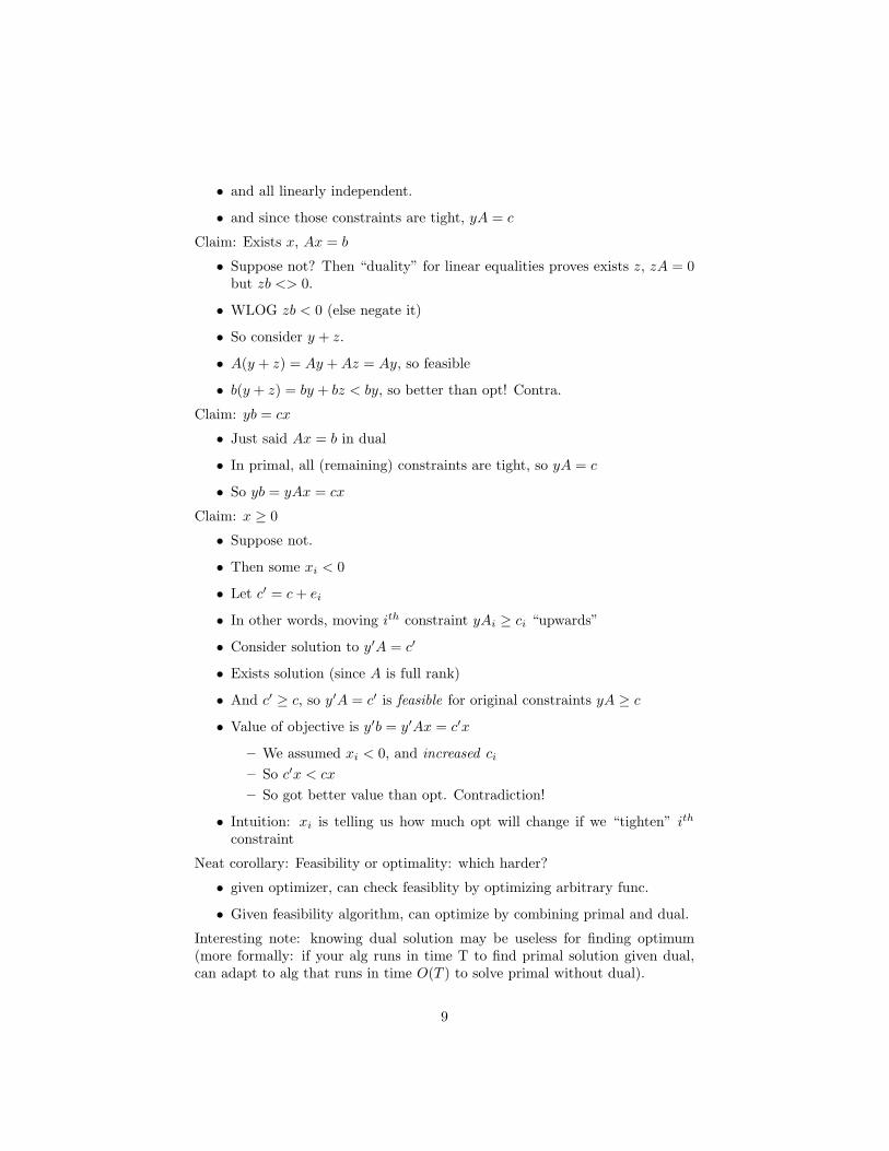
Claim: Exists x, Ax = b
• Suppose not? Then “duality” for linear equalities proves exists z, zA = 0but zb <> 0.
• WLOG zb < 0 (else negate it)
• So consider y + z.
• A(y + z) = Ay + Az = Ay, so feasible
• b(y + z) = by + bz < by, so better than opt! Contra.
Claim: yb = cx
• Just said Ax = b in dual
• In primal, all (remaining) constraints are tight, so yA = c
• So yb = yAx = cx
Claim: x ≥ 0
• Suppose not.
• Then some xi < 0
• Let c′ = c + ei
• In other words, moving ith constraint yAi ≥ ci “upwards”
• Consider solution to y′A = c′
• Exists solution (since A is full rank)
• And c′ ≥ c, so y′A = c′ is feasible for original constraints yA ≥ c
• Value of objective is y′b = y′Ax = c′x
– We assumed xi < 0, and increased ci
– So c′x < cx
– So got better value than opt. Contradiction!
• Intuition: xi is telling us how much opt will change if we “tighten” ith
constraint
Neat corollary: Feasibility or optimality: which harder?
• given optimizer, can check feasiblity by optimizing arbitrary func.
• Given feasibility algorithm, can optimize by combining primal and dual.
Interesting note: knowing dual solution may be useless for finding optimum(more formally: if your alg runs in time T to find primal solution given dual,can adapt to alg that runs in time O(T ) to solve primal without dual).
9
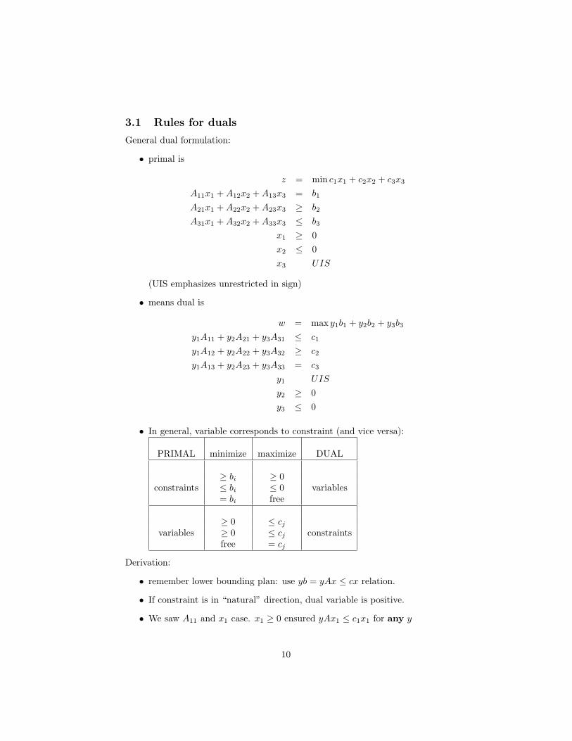
3.1 Rules for duals
General dual formulation:
• primal is
z = min c1x1 + c2x2 + c3x3
A11x1 + A12x2 + A13x3 = b1
A21x1 + A22x2 + A23x3 ≥ b2
A31x1 + A32x2 + A33x3 ≤ b3
x1 ≥ 0x2 ≤ 0x3 UIS
(UIS emphasizes unrestricted in sign)
• means dual is
w = max y1b1 + y2b2 + y3b3
y1A11 + y2A21 + y3A31 ≤ c1
y1A12 + y2A22 + y3A32 ≥ c2
y1A13 + y2A23 + y3A33 = c3
y1 UIS
y2 ≥ 0y3 ≤ 0
• In general, variable corresponds to constraint (and vice versa):
PRIMAL minimize maximize DUAL
≥ bi ≥ 0constraints ≤ bi ≤ 0 variables
= bi free
≥ 0 ≤ cj
variables ≥ 0 ≤ cj constraintsfree = cj
Derivation:
• remember lower bounding plan: use yb = yAx ≤ cx relation.
• If constraint is in “natural” direction, dual variable is positive.
• We saw A11 and x1 case. x1 ≥ 0 ensured yAx1 ≤ c1x1 for any y
10
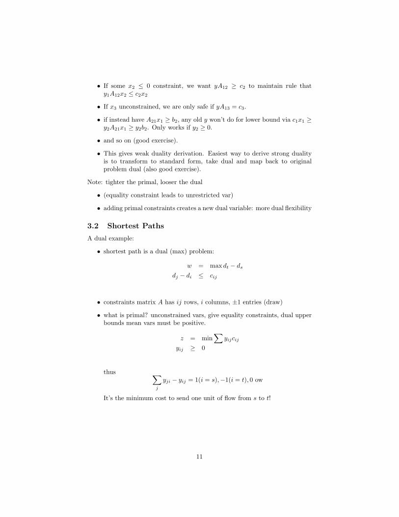
• If some x2 ≤ 0 constraint, we want yA12 ≥ c2 to maintain rule thaty1A12x2 ≤ c2x2
• If x3 unconstrained, we are only safe if yA13 = c3.
• if instead have A21x1 ≥ b2, any old y won’t do for lower bound via c1x1 ≥y2A21x1 ≥ y2b2. Only works if y2 ≥ 0.
• and so on (good exercise).
• This gives weak duality derivation. Easiest way to derive strong dualityis to transform to standard form, take dual and map back to originalproblem dual (also good exercise).
Note: tighter the primal, looser the dual
• (equality constraint leads to unrestricted var)
• adding primal constraints creates a new dual variable: more dual flexibility
3.2 Shortest Paths
A dual example:
• shortest path is a dual (max) problem:
w = max dt − ds
dj − di ≤ cij
• constraints matrix A has ij rows, i columns, ±1 entries (draw)
• what is primal? unconstrained vars, give equality constraints, dual upperbounds mean vars must be positive.
z = min∑
yijcij
yij ≥ 0
thus ∑j
yji − yij = 1(i = s),−1(i = t), 0 ow
It’s the minimum cost to send one unit of flow from s to t!
11
4 Complementary Slackness
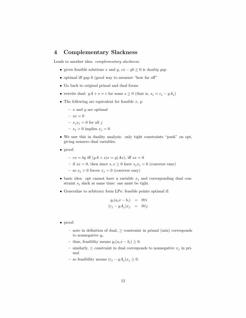
Leads to another idea: complementary slackness:
• given feasible solutions x and y, cx− yb ≥ 0 is duality gap.
• optimal iff gap 0 (good way to measure “how far off”
• Go back to original primal and dual forms
• rewrite dual: yA + s = c for some s ≥ 0 (that is, sj = cj − yAj)
• The following are equivalent for feasible x, y:
– x and y are optimal
– sx = 0
– xjsj = 0 for all j
– sj > 0 implies xj = 0
• We saw this in duality analysis: only tight constraints “push” on opt,giving nonzero dual variables.
• proof:
– cx = by iff (yA + s)x = y(Ax), iff sx = 0
– if sx = 0, then since s, x ≥ 0 have sjxj = 0 (converse easy)
– so sj > 0 forces xj = 0 (converse easy)
• basic idea: opt cannot have a variable xj and corresponding dual con-straint sj slack at same time: one must be tight.
• Generalize to arbitrary form LPs: feasible points optimal if:
yi(aix− bi) = 0∀i(cj − yAj)xj = 0∀j
• proof:
– note in definition of dual, ≥ constraint in primal (min) correspondsto nonnegative yi.
– thus, feasiblity means yi(aix− bi) ≥ 0.
– similarly, ≤ constraint in dual corresponds to nonnegative xj in pri-mal
– so feasibility means (cj − yAj)xj ≥ 0.
12
– Also,∑yi(aix− bi) + (cj − yAj)xj = yAx− yb + cx− yAx
= cx− yb
= 0
at opt. But since just argued all terms are nonnegative, all must be0
– conversely, if all are 0, then cx = by, so we are optimal
Let’s take some duals.Max-Flow min-cut theorem:
• modify to circulation to simplify
• primal problem: create infinite capacity (t, s) arc
P = max∑w
xts∑w
xvw − xwv = 0
xvw ≤ uvw
xvw ≥ 0
• dual problem: vars zv dual to balance constraints, yvw dual to capacityconstraints.
D = min∑vw
yvwuvw
yvw ≥ 0zv − zw + yvw ≥ 0
zt − zs + yts ≥ 1
• Think of yvw as “lengths”
• note yts = 0 since otherwise dual infinite. so zt − zs ≥ 1.
• rewrite as zw ≤ zv + yvw.
• deduce yvw are edge lengths, zv are “distances”
• In particular, can substract zs from everything without changing feasibility(subs cancel)
• Now zv is upper bound on distance from source to v.
• So, are trying to maximize source-sink distance
13
– Good justification for shortest aug path, blocking flows
• sanity check: mincut: assign length 1 to each mincut edge
• unfortunately, might have noninteger dual optimum.
• let S = v | zv < 1 (so s ∈ S, t /∈ S)
• use complementary slackness:
– if (v, w) leaves S, then yvw ≥ zw − zv > 0, so xvw = uvw, (tight) i.e.(v, w) saturated.
– if (v, w) enters S, then zv > zw. Also know yvw ≥ 0; add equationsand get zv + yvw > zw i.e. slack.
– so xwv = 0– in other words: all leaving edges saturated, all coming edges empty.
• now just observe that value of flow equals value crossing cut equals valueof cut.
Min cost circulation: change the objective function associated with max-flow.
• primal:
z = min∑
cvwxvw∑w
xvw − xwv = 0
xvw ≤ uvw
xvw ≥ 0
• as before, dual: variable yvw for capacity constraint on fvw, zv for balance.
• Change to primal min problem flips sign constraint on yvw
• What does change in primal objective mean for dual? Different constraintbounds!
max∑
yvwuvw
zv − zw + yvw ≤ cvw
yvw ≤ 0zv UIS
• rewrite dual: pv = −zv
max∑
yvwuvw
yvw ≤ 0yvw ≤ cvw + pv − pw = c(p)
vw
14
• Note: yvw ≤ 0 says the objective function is the sum of the negativeparts of the reduced costs (positive ones get truncated to 0)
• Note: optimum ≤ 0 since of course can set y = 0. Since since zerocirculation is primal feasible.
• complementary slackness.
– Suppose fvw < uvw.
– Then dual variable yvw = 0
– So c(p)ij ≥ 0
– Thus c(p)ij < 0 implies fij = uij
– that is, all negative reduced cost arcs saturated.
– on the other hand, suppose c(p)ij > 0
– then constraint on zij is slack
– so fij = 0
– that is, all positive reduced arcs are empty.
5 Algorithms
5.1 Simplex
vertices in standard form/bases:
• Without loss of generality make A have full row rank (define):
– find basis in rows of A, say a1, . . . , ak
– any other a` is linear combo of those.
– so a`x =∑
λiaix
– so better have bl =∑
λiai if any solution.
– if so, anything feasible for a1, . . . , a` feasible for all.
• m constraints Ax = b all tight/active
• given this, need n−m of the xi ≥ 0 constraints
• also, need them to form a basis with the ai.
• write matrix of tight constraints, first m rows then identity matrix
• need linearly independent rows
• equiv, need linearly independent columns
• but columns are linearly independent iff m columns of A including allcorresp to nonzero x are linearly independent
15
• gives other way to define a vertex: x is vertex if
– Ax = b
– m linearly independent columns of A include all xj 6= 0
This set of m columns is called a basis.
• xj of columns called basic set B, others nonbasic set N
• given bases, can compute x:
– AB is basis columns, m×m and full rank.
– solve ABxB = b, set other xN = 0.
– note can have many bases for same vertex (choice of 0 xj)
Summary: x is vertex of P if for some basis B,
• xN = 0
• AB nonsingular
• A−1B b ≥ 0
Simplex method:
• start with a basic feasible soluion
• try to improve it
• rewrite LP: min cBxB + cNxN , ABxB + ANxN = b, x ≥ 0
• B is basis for bfs
• since ABxB = b−ANxN , so xB = A−1B (b−ANxN ), know that
cx = cBxB + cNxN
= cBA−1B (b−ANxN ) + cNxN
= cBA−1B b + (cN − cBA−1
B AN )xN
• reduced cost c̃N = cN − cBA−1B AN
• if no c̃j < 0, then increasing any xj increases cost (may violate feasiblityfor xB , but who cares?), so are at optimum!
• if some c̃j < 0, can increase xj to decrease cost
• but since xB is func of xN , will have to stop when xB hits a constraint.
• this happens when some xi, i ∈ B hits 0.
16
• we bring j into basis, take i out of basis.
• we’ve moved to an adjacent basis.
• called a pivot
• show picture
Notes:
• Need initial vertex. How find?
• maybe some xi ∈ B already 0, so can’t increase xj , just pivot to same objfunction.
• could lead to cycle in pivoting, infinite loop.
• can prove exist noncycling pivots (eg, lexicographically first j and i)
• no known pivot better than exponential time
• note traverse path of edges over polytope. Unknown what shortest suchpath is
• Hirsh conjecture: path of m− d pivots exists.
• even if true, simplex might be bad because path might not be monotonein objective function.
• certain recent work has shown nlog n bound on path length
5.2 Simplex and Duality
• defined reduced costs of nonbasic vars N by
c̃N = cN − cBA−1B AN
and argued that when all c̃N ≥ 0, had optimum.
• Define y = cBA−1B (so of course cB = yAB)
• nonegative reduced costs means cN ≥ yAN
• put together, see yA ≤ c so y is dual feasible
• but, yb = cBA−1B b = cBxB = cx (since xN = 0)
• so y is dual optimum.
• more generally, y measures duality gap for current solution!
• another way to prove duality theorem: prove there is a terminating (noncycling) simplex algorithm.
17
5.3 Polynomial Time Bounds
We know a lot about structure. And we’ve seen how to verify optimality inpolynomial time. Now turn to question: can we solve in polynomial time?Yes, sort of (Khachiyan 1979):
• polynomial algorithms exist
• strongly polynomial unknown.
Claim: all vertices of LP have polynomial size.
• vertex is bfs
• bfs is intersection of n constraints ABx = b
• invert matrix.
Now can prove that feasible alg can optimize a different way:
• use binary search on value z of optimum
• add constraint cx ≤ z
• know opt vertex has poly number of bits
• so binary search takes poly (not logarithmic!) time
• not as elegant as other way, but one big advantage: feasiblity test overbasically same polytope as before. Might have fast feasible test for thiscase.
6 Ellipsoid
Lion hunting in the desert.
• bolzano wierstrauss theorem—proves certain sequence has a subsequencewith a limit by repeated subdividing of intervals to get a point in the
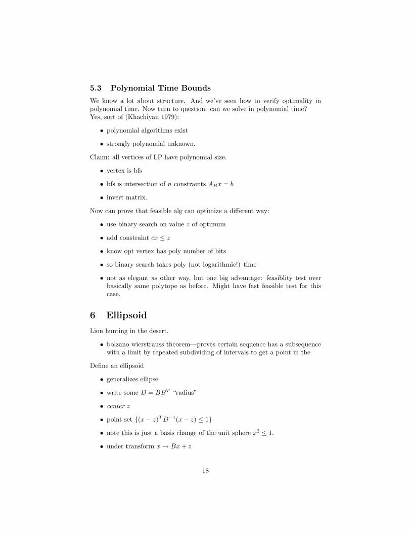
Define an ellipsoid
• generalizes ellipse
• write some D = BBT “radius”
• center z
• point set {(x− z)T D−1(x− z) ≤ 1}
• note this is just a basis change of the unit sphere x2 ≤ 1.
• under transform x → Bx + z
18
Outline of algorithm:
• goal: find a feasible point for P = {Ax ≤ b}
• start with ellipse containing P , center z
• check if z ∈ P
• if not, use separating hyperplane to get 1/2 of ellipse containing P
• find a smaller ellipse containing this 1/2 of original ellipse
• until center of ellipse is in P .
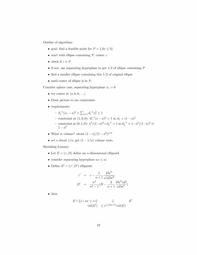
Consider sphere case, separating hyperplane x1 = 0
• try center at (a, 0, 0, . . .)
• Draw picture to see constraints
• requirements:
– d−11 (x1 − a)2 +
∑i>1 d−1
i x2i ≤ 1
– constraint at (1, 0, 0): d−11 (x− a)2 = 1 so d1 = (1− a)2
– constraint at (0, 1, 0): a2/(1−a)2+d−12 = 1 so d−1
2 = 1−a2/(1−a)2 ≈1− a2
• What is volume? about (1− a)/(1− a2)n/2
• set a about 1/n, get (1− 1/n) volume ratio.
Shrinking Lemma:
• Let E = (z,D) define an n-dimensional ellipsoid
• consider separating hyperplane ax ≤ az
• Define E′ = (z′, D′) ellipsoid:
z′ = z − 1n + 1
DaT
√aDaT
D′ =n2
n2 − 1(D − 2
n + 1DaT aD
aDaT)
• then
E ∩ {x | ax ≤ ez} ⊆ E′
vol(E′) ≤ e1/(2n+1)vol(E)
19
• for proof, first show works with D = I and z = 0. new ellipse:
z′ = − 1n + 1
D′ =n2
n2 − 1(I − 2
n + 1I11)
and volume ratio easy to compute directly.
• for general case, transform to coordinates where D = I (using new basisB), get new ellipse, transform back to old coordinates, get (z′, D′) (notetransformation don’t affect volume ratios.
So ellipsoid shrinks. Now prove 2 things:
• needn’t start infinitely large
• can’t get infinitely small
Starting size:
• recall bounds on size of vertices (polynomial)
• so coords of vertices are exponential but no larger
• so can start with sphere with radius exceeding this exponential bound
• this only uses polynomial values in D matrix.
• if unbounded, no vertices of P , will get vertex of box.
Ending size:
• convenient to assume that polytope full dimensional
• if so, it has n + 1 affinely indpendent vertices
• all the vertices have poly size coordinates
• so they contain a box whose volume is a poly-size number (computable asdeterminant of vertex coordinates)
Put together:
• starting volume 2nO(1)
• ending volume 2−nO(1)
• each iteration reduces volume by e1/(2n+1) factor
• so 2n + 1 iters reduce by e
• so nO(1) reduce by enO(1)
20
• at which point, ellipse doesn’t contain P , contra
• must have hit a point in P before.
Justifying full dimensional:
• take {Ax ≤ b}, replace with P ′ = {Ax ≤ b + ε} for tiny ε
• any point of P is an interior of P ′, so P ′ full dimensional (only haveinterior for full dimensional objects)
• P empty iff P ′ is (because ε so small)
• can “round” a point of P ′ to P .
Infinite precision:
• built a new ellipsoid each time.
• maybe its bits got big?
• no.
6.1 Separation vs Optimization
Notice in ellipsoid, were only using one constraint at a time.
• didn’t matter how many there were.
• didn’t need to see all of them at once.
• just needed each to be represented in polynomial size.
• so ellipsoid works, even if huge number of constraints, so long as haveseparation oracle: given point not in P , find separating hyperplane.
• of course, feasibility is same as optimize, so can optimize with sep oracletoo.
• this is on a polytope by polytope basis. If can separate a particular poly-tope, can optimize over that polytope.
This is very useful in many applications. e.g. network design.
7 Interior Point
Ellipsoid has problems in practice (O(n6) for one). So people developed a dif-ferent approach that has been extremely successful.What goes wrong with simplex?
• follows edges of polytope
21
• complex stucture there, run into walls, etc
• interior point algorithms stay away from the walls, where structure sim-pler.
• Karmarkar did the first one (1984); we’ll descuss one by Ye
7.1 Potential Reduction
Potential function:
• Idea: use a (nonlinear) potential function that is minimized at opt butalso enforces feasibility
• use gradient descent to optimize the potential function.
• Recall standard primal {Ax = b, x ≥ 0} and dual yA + s = c, s ≥ 0.
• duality gap sx
• Use logarithmic barrier function
G(x, s) = q lnxs−∑
lnxj −∑
ln sj
and try to minimize it (pick q in a minute)
• first term forces duality gap to get small
• second and third enforce positivity
• note barrier prevents from ever hitting optimum, but as discussed aboveok to just get close.
Choose q so first term dominates, guarantees good G is good xs
• G(x, s) small should mean xs small
• xs large should mean G(x, s) large
• write G = ln(xs)q/∏
xjsj
• xs > xjsj , so (xs)n >∏
xjsj . So taking q > n makes top term dominate,G > lnxs
How minimize potential function? Gradient descent.
• have current (x, s) point.
• take linear approx to potential function around (x, s)
• move to where linear approx smaller (−∇xG)
• deduce potential also went down.
22
• crucial: can only move as far as linear approximation accurate
Firs wants big q, second small q. Compromise at n +√
n, gives O(L√
n) itera-tions.Must stay feasible:
• Have gradient g = ∇xG
• since potential not minimized, have reasonably large gradient, so a smallstep will improve potential a lot. picture
• want to move in direction of G, but want to stay feasilbe
• project G onto nullspace(A) to get d
• then A(x + d) = Ax = b
• also, for sufficiently small step, x ≥ 0
• potential reduction proportional to length of d
• problem if d too small
• In that case, move s (actually y) by g − d which will be big.
• so can either take big primal or big dual step
• why works? Well, d (perpendicular to A) has Ad = 0, so good primalmove.
• converseley, part spanned by A has g − d = wA,
• so can choose y′ = y+w and get s′ = c−Ay′ = c−Ay−(g−d) = s−(g−d).
• note dG/dxj = sj/(xs)− 1/xj
• and dG/dsj = xj/(xs)− 1/sj = (xj/sj)dG/dxj ≈ dG/dxj
23


![lecture24-1 - Massachusetts Institute of Technologycourses.csail.mit.edu/6.889/fall11/lectures/L24.pdf · [Nd05] J. Ne set ril and P. Ossona de Mendez. Tree depth, subgraph col-oring](https://static.fdocuments.in/doc/165x107/5ba64b1009d3f22f1b8b9c9e/lecture24-1-massachusetts-institute-of-nd05-j-ne-set-ril-and-p-ossona.jpg)