1

Lecture 14: Jointly Distributed Random Variables

Devore, Ch. 5.1 and 5.2

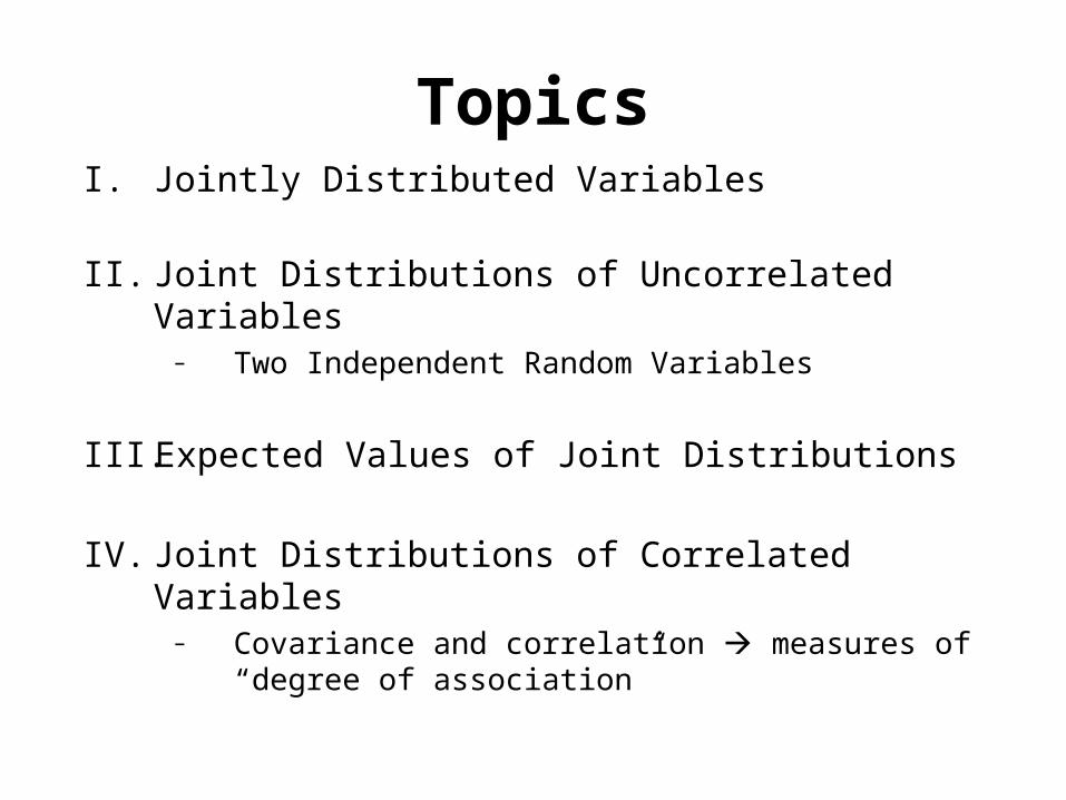
TopicsI. Jointly Distributed Variables

II. Joint Distributions of Uncorrelated Variables

– Two Independent Random Variables

III. Expected Values of Joint Distributions

IV. Joint Distributions of Correlated Variables – Covariance and correlation measures of

“degree of association”

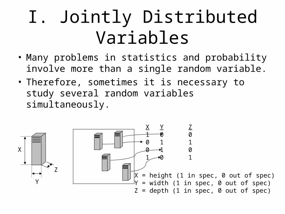
I. Jointly Distributed Variables

• Many problems in statistics and probability involve more than a single random variable.

• Therefore, sometimes it is necessary to study several random variables simultaneously.

X Y Z1 0 00 1 10 1 01 0 1

X = height (1 in spec, 0 out of spec)Y = width (1 in spec, 0 out of spec)Z = depth (1 in spec, 0 out of spec)

X

Y

Z

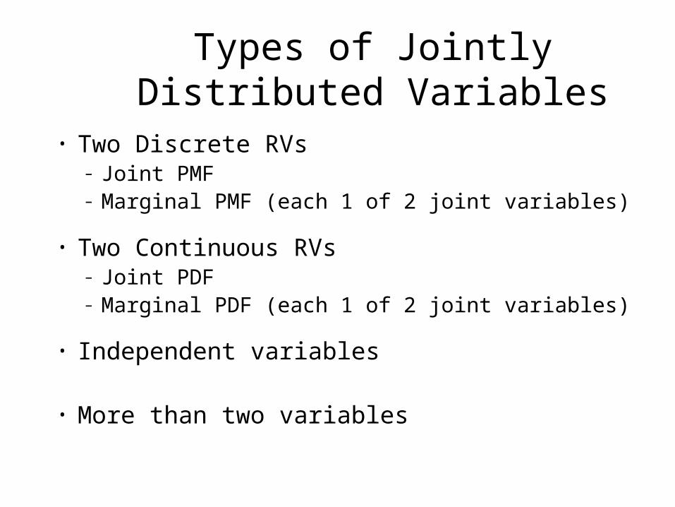
Types of Jointly Distributed Variables

• Two Discrete RVs– Joint PMF– Marginal PMF (each 1 of 2 joint variables)

• Two Continuous RVs– Joint PDF– Marginal PDF (each 1 of 2 joint variables)

• Independent variables

• More than two variables

Joint Distribution – Two Discrete RV’s

Joint PMFLet X and Y represent 2

discrete rv’s on space SpXY(x,y) >= 0

pXY(x,y) = P(X=x, Y=y)

Marginal PMFTo obtain a marginal pmf for say X=100,

P(100,y) - you compute prob for all possible y values.

xy

yx

yxpyp

yxpxp

),()(

),()(

1),( x y

XY yxp

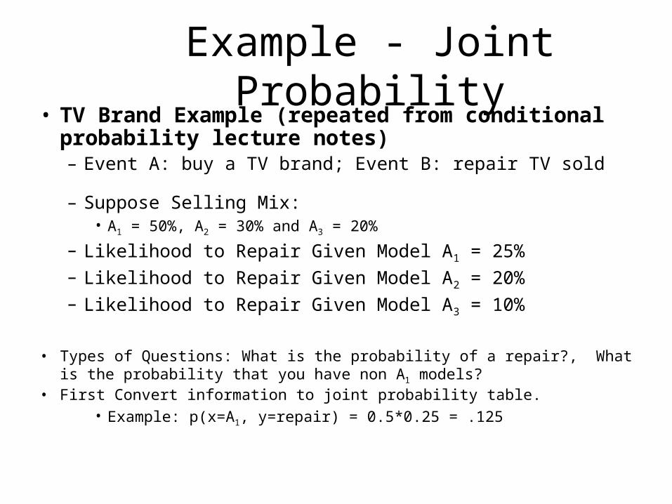
Example - Joint Probability• TV Brand Example (repeated from conditional

probability lecture notes)– Event A: buy a TV brand; Event B: repair TV sold

– Suppose Selling Mix: • A1 = 50%, A2 = 30% and A3 = 20%

– Likelihood to Repair Given Model A1 = 25%– Likelihood to Repair Given Model A2 = 20%– Likelihood to Repair Given Model A3 = 10%

• Types of Questions: What is the probability of a repair?, What is the probability that you have non A1 models?

• First Convert information to joint probability table.• Example: p(x=A1, y=repair) = 0.5*0.25 = .125

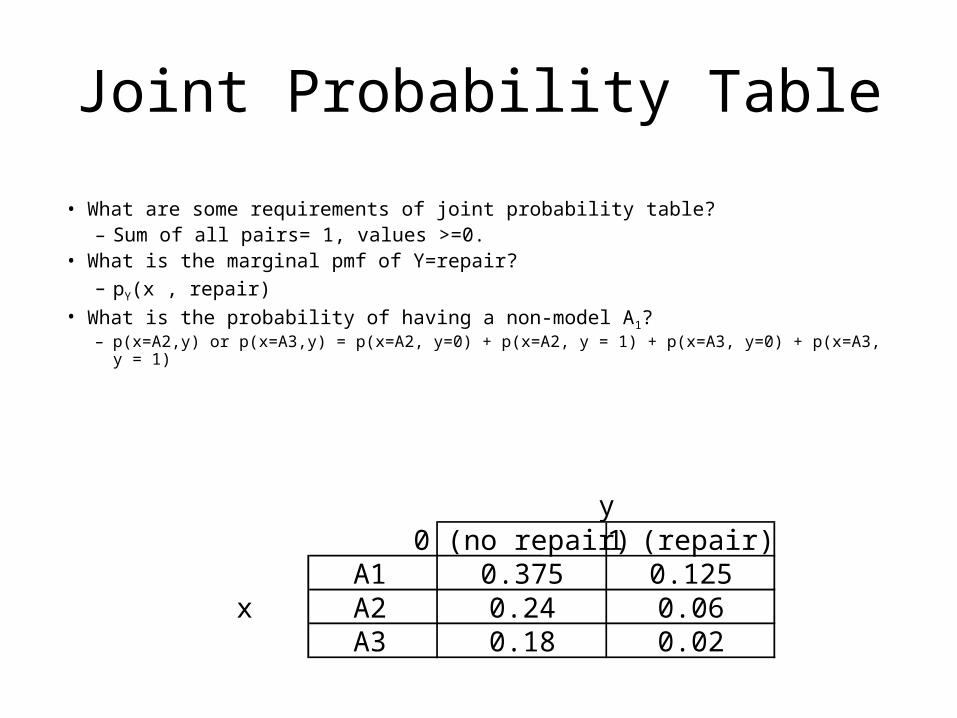
Joint Probability Table

• What are some requirements of joint probability table?– Sum of all pairs= 1, values >=0.

• What is the marginal pmf of Y=repair?– pY(x , repair)

• What is the probability of having a non-model A1?– p(x=A2,y) or p(x=A3,y) = p(x=A2, y=0) + p(x=A2, y = 1) + p(x=A3, y=0) + p(x=A3, y = 1)

0 (no repair) 1 (repair)A1 0.375 0.125

x A2 0.24 0.06A3 0.18 0.02

y

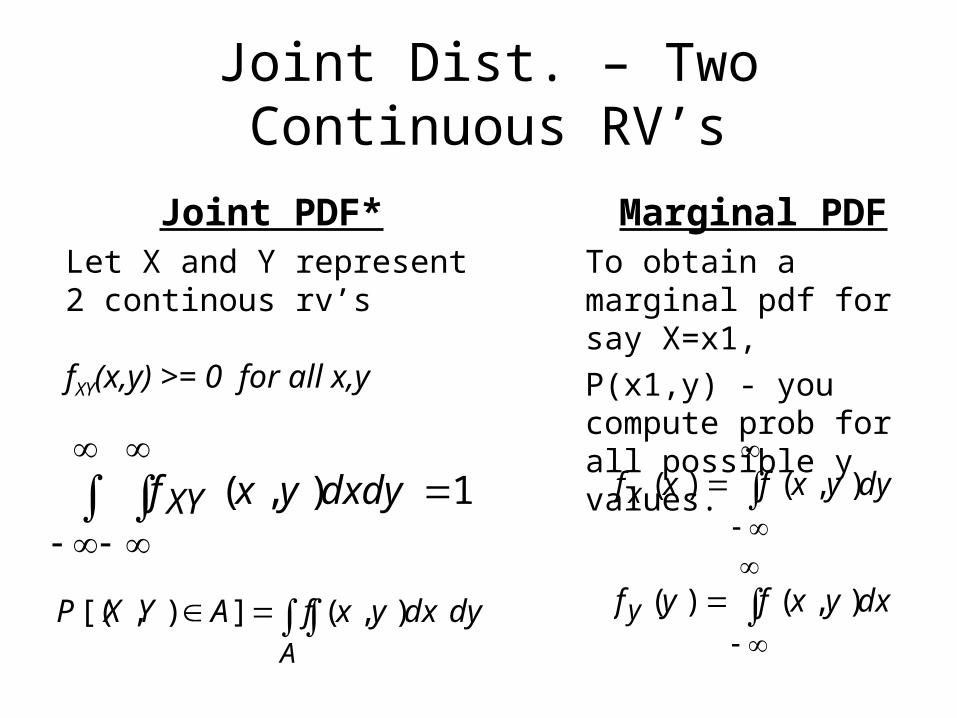
Joint Dist. – Two Continuous RV’s

Joint PDF*Let X and Y represent 2 continous rv’s

fXY(x,y) >= 0 for all x,y

Marginal PDFTo obtain a marginal pdf for say X=x1,

P(x1,y) - you compute prob for all possible y values.

),()(

),()(

dxyxfyf

dyyxfxf

y

x1),(

dxdyyxfXY

A

dydxyxfAYXP ),(]),[(

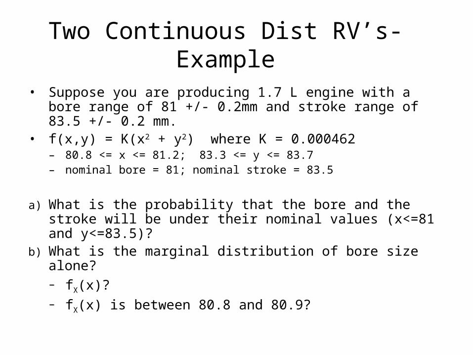
Two Continuous Dist RV’s- Example

• Suppose you are producing 1.7 L engine with a bore range of 81 +/- 0.2mm and stroke range of 83.5 +/- 0.2 mm.

• f(x,y) = K(x2 + y2) where K = 0.000462– 80.8 <= x <= 81.2; 83.3 <= y <= 83.7– nominal bore = 81; nominal stroke = 83.5

a) What is the probability that the bore and the stroke will be under their nominal values (x<=81 and y<=83.5)?

b) What is the marginal distribution of bore size alone?– fX(x)?– fX(x) is between 80.8 and 80.9?

10

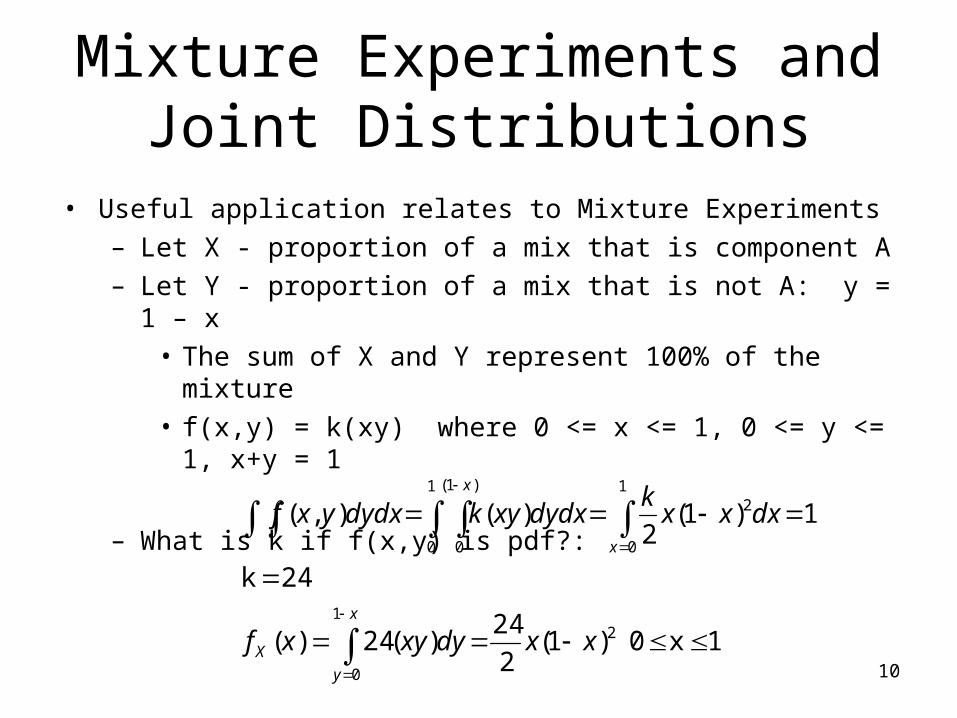
Mixture Experiments and Joint Distributions

• Useful application relates to Mixture Experiments– Let X - proportion of a mix that is component A– Let Y - proportion of a mix that is not A: y = 1 – x

• The sum of X and Y represent 100% of the mixture• f(x,y) = k(xy) where 0 <= x <= 1, 0 <= y <= 1, x+y = 1

– What is k if f(x,y) is pdf?:

1x 0 )1(2

24)(24)(

24 k

1)1(2

)(),(

1

0

2

1

0

21

0

)1(

0

x

y

X

x

x

xxdyxyxf

dxxxk

dydxxykdydxyxf

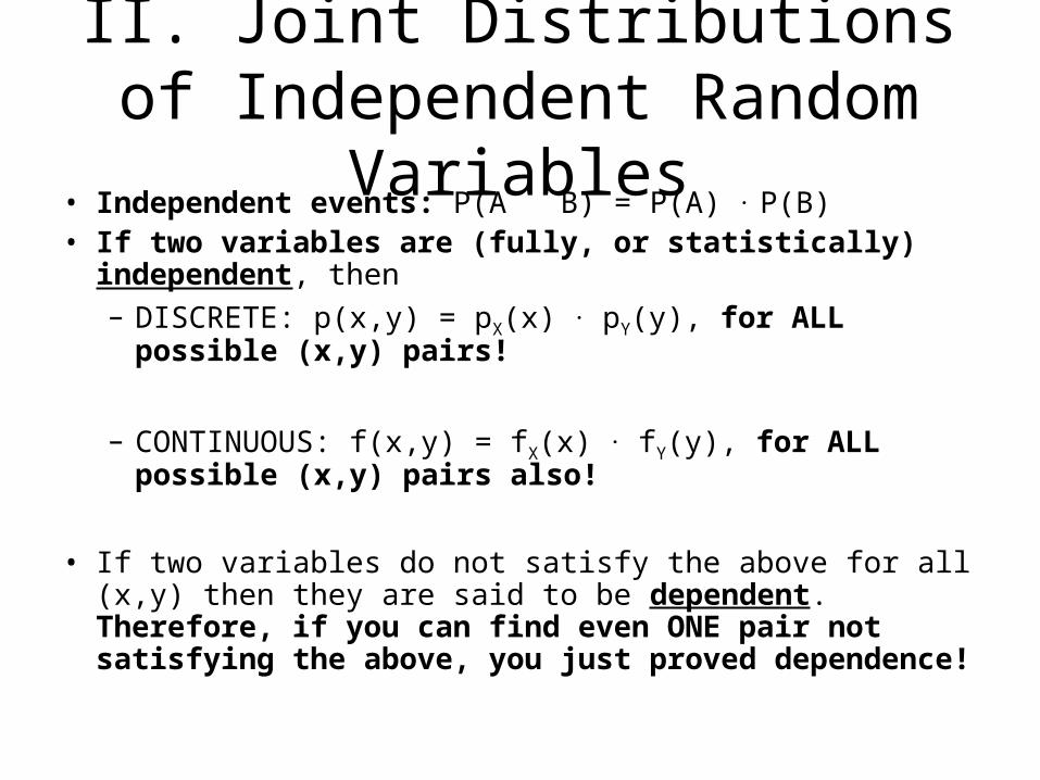
II. Joint Distributions of Independent Random

Variables• Independent events: P(A B) = P(A) . P(B) • If two variables are (fully, or statistically) independent,

then– DISCRETE: p(x,y) = pX(x) . pY(y), for ALL possible (x,y)

pairs!

– CONTINUOUS: f(x,y) = fX(x) . fY(y), for ALL possible (x,y) pairs also!

• If two variables do not satisfy the above for all (x,y) then they are said to be dependent. Therefore, if you can find even ONE pair not satisfying the above, you just proved dependence!

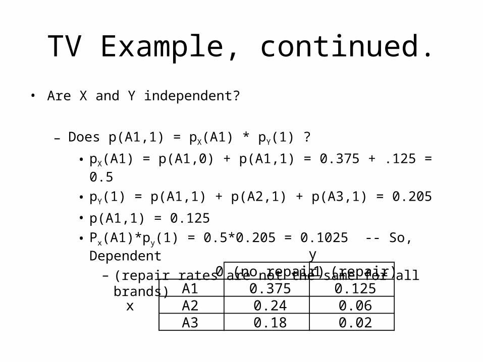
TV Example, continued.

• Are X and Y independent?

– Does p(A1,1) = pX(A1) * pY(1) ?

• pX(A1) = p(A1,0) + p(A1,1) = 0.375 + .125 = 0.5

• pY(1) = p(A1,1) + p(A2,1) + p(A3,1) = 0.205

• p(A1,1) = 0.125

• Px(A1)*py(1) = 0.5*0.205 = 0.1025 -- So, Dependent

– (repair rates are not the same for all brands)

0 (no repair) 1 (repair)A1 0.375 0.125

x A2 0.24 0.06A3 0.18 0.02

y

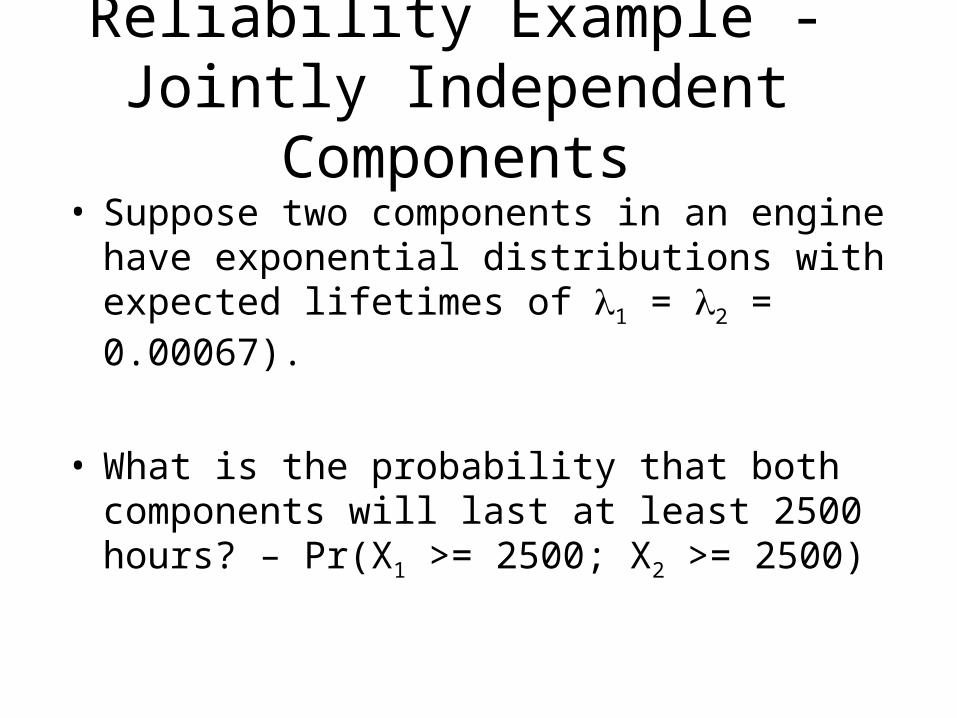
Reliability Example - Jointly Independent Components• Suppose two components in an engine have

exponential distributions with expected lifetimes of 1 = 2 = 0.00067).

• What is the probability that both components will last at least 2500 hours? – Pr(X1 >= 2500; X2 >= 2500)

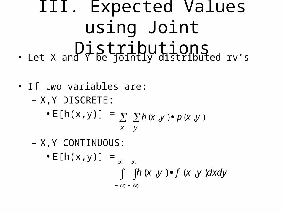
III. Expected Values using Joint Distributions

• Let X and Y be jointly distributed rv’s

• If two variables are:– X,Y DISCRETE:

• E[h(x,y)] =

– X,Y CONTINUOUS:• E[h(x,y)] =

yx

yxpyxh ),(),(

dxdyyxfyxh ),(),(

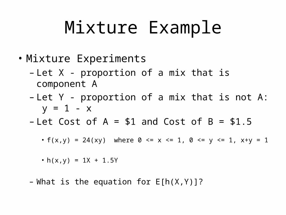
Mixture Example

• Mixture Experiments– Let X - proportion of a mix that is component A– Let Y - proportion of a mix that is not A: y = 1 -

x– Let Cost of A = $1 and Cost of B = $1.5

• f(x,y) = 24(xy) where 0 <= x <= 1, 0 <= y <= 1, x+y = 1

• h(x,y) = 1X + 1.5Y

– What is the equation for E[h(X,Y)]?

IV. Joint Distributions of Related Variables

• Suppose X and Y are not independent but dependent.

• Useful Question: what is the degree of association between X and Y?

– Measures of degree of association:• Covariance• Correlation

Covariance of X and Y

• Covariance between two rv’s X and Y is:– Cov(X,Y) = E[(X-x)(Y-y)]

• Covariance Results:– If X and Y tend to both be greater than their

respective means at the same time, then the covariance becomes a large positive number.

– If X and Y tend to both be lower than their respective means at the same time, then the covariance becomes a large negative number.

– If X and Y tend to cancel one another, then the covariance should be near 0.

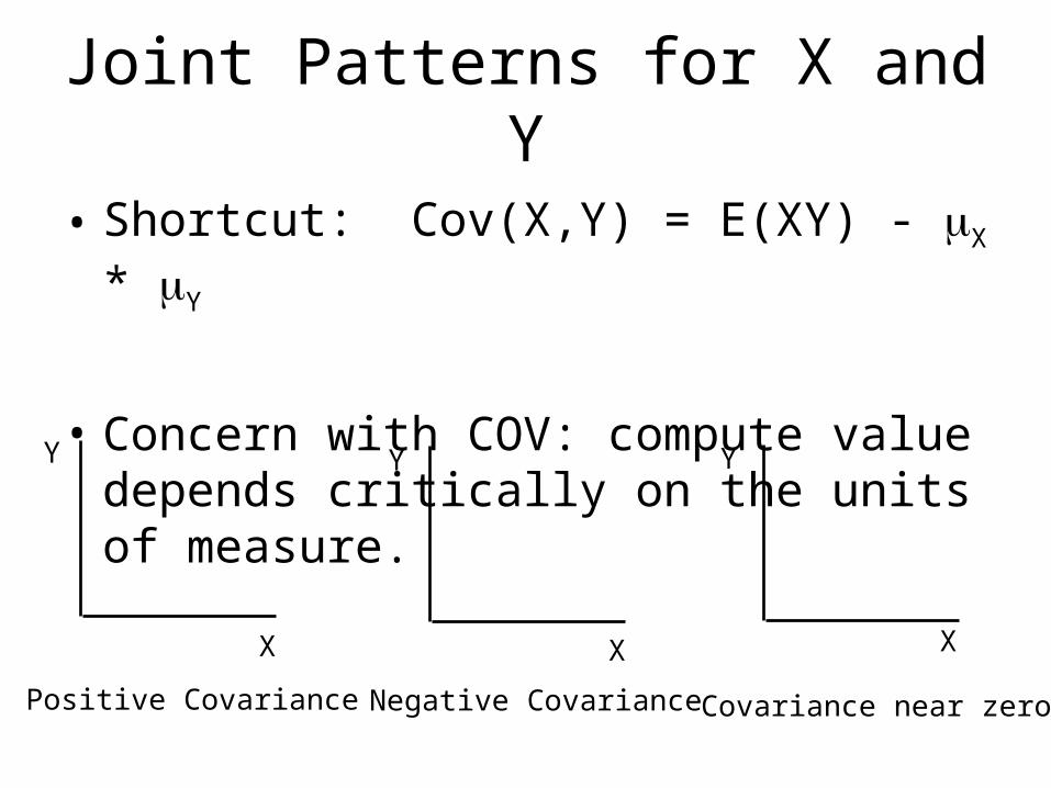
Joint Patterns for X and Y

• Shortcut: Cov(X,Y) = E(XY) - X * Y

• Concern with COV: compute value depends critically on the units of measure.

Positive Covariance Negative Covariance Covariance near zero

X X X

Y Y Y

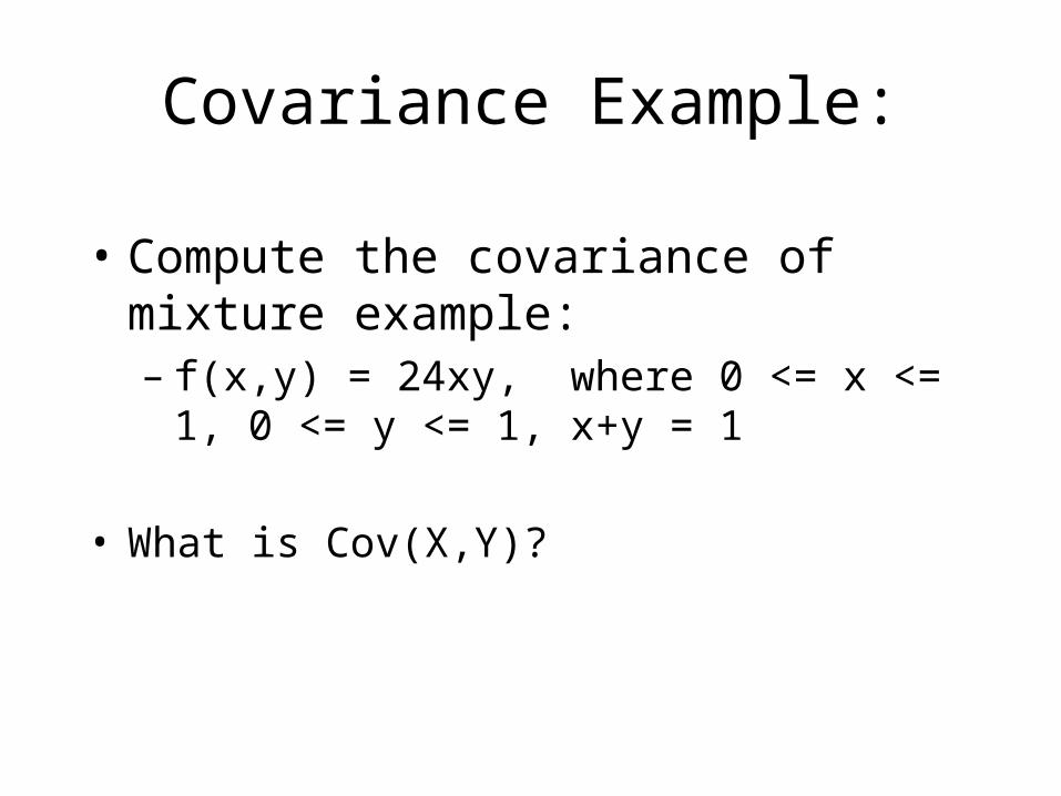
Covariance Example:

• Compute the covariance of mixture example:– f(x,y) = 24xy, where 0 <= x <= 1, 0 <= y <=

1, x+y = 1

• What is Cov(X,Y)?

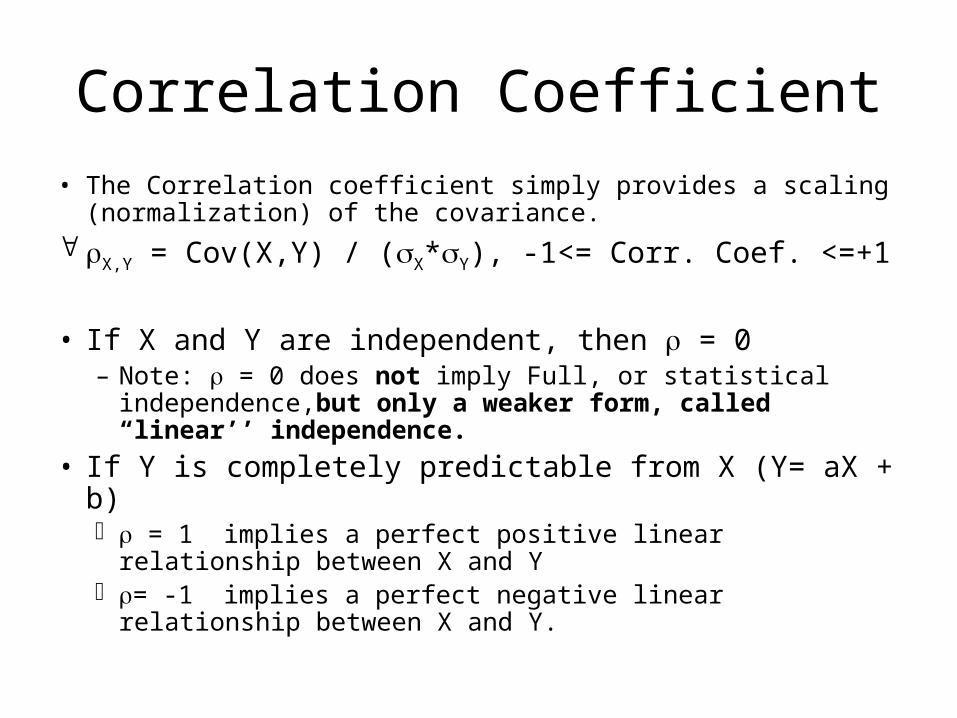
Correlation Coefficient• The Correlation coefficient simply provides a scaling

(normalization) of the covariance.

X,Y = Cov(X,Y) / (X*Y), -1<= Corr. Coef. <=+1

• If X and Y are independent, then = 0– Note: = 0 does not imply Full, or statistical

independence,but only a weaker form, called “linear’’ independence.

• If Y is completely predictable from X (Y= aX + b) = 1 implies a perfect positive linear relationship between X

and Y = -1 implies a perfect negative linear relationship between

X and Y.

Answers• Slide 7

– pY(x , repair)=0.125+0.06+0.02=0.205– p(x=A2, y=0) + p(x=A2, y = 1) + p(x=A3, y=0) + p(x=A3, y =

1)=0.24+.06+.18+.02=0.5

• Slide 9– part a:

– part b: 0.0001848 x2 + 1.288• Slide 13

– R(2500)=e^(-lambda*t)=e^(-0.00067*2500)=0.187 (each component)

– Pr(X1 >= 2500; X2 >= 2500)=0.187*0.187=0.035• Slide 15

2494.05.83

3.83

81

8.80

22 dxdyyxK

dydxxyyxx

1

0

1

0

245.1

Answers

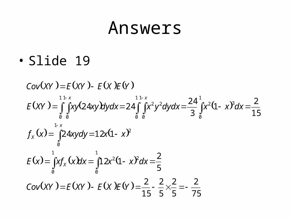
• Slide 19

75

2

5

2

5

2

15

2

5

2112

11224

15

21

3

242424

1

0

221

0

1

0

2

1

0

3221

0

1

0

21

0

1

0

YEXEXYEXYCov

dxxxdxxxfxE

xxxydyxf

dxxxdydxyxdydxxyxyXYE

YEXEXYEXYCov

X

x

X

xx