1

Lecture 7: Discrete Random

Variables and their Distributions

Devore, Ch. 3.1 - 3.3

Topics

I. Random variables– Definition– Types of R.V.’s

II. Probability distributions for discrete random variables

– Probability mass function– Cumulative distribution (mass) function

III. Expected values of discrete random variables– Expected values (r.v., function, rules)– Variance (r.v., rules)

I. Random variables

• Definition: A random variable (rv) is a rule that associates a value with each of the possible outcomes of an event

– Example: if X is a rv that defines the number of heads that we may obtain when we flip 3 coins, then X can take 4 values: 0,1,2,3

Bernoulli random variables

• A random variable (rv) whose values are only 0 or 1 is called a Bernoulli random variable

– Common Notation: 0 – Fail (F); 1 – Success (S) – Example: Suppose X is a rv that indicates

whether a user can login to a computer system, either all ports are busy (Fail) or there is at least one port free (Success), then X can take 2 values, 0 or 1:

• X (S)=1, X(F)=0

Discrete and Continuous R.V.’s

• A discrete R.V. has whole unit values either in a finite set or listed in an ascending infinite sequence (first element, second element, and so on)– Example: X is discrete R.V. defined to be: the #

of pumps in use at a gas station

• A continuous R.V. takes any value in a given interval. It has an infinite (or nearly infinite) set of possible values in that interval.– Example: Z is a continuous R.V., defined as the

speed at which a professional tennis player hits his/her first serve

Exercise 1

• Let X = the number of nonzero digits in a randomly selected zip code. What are the possible values of X ?

Give three possible outcomes and their associated X values

Different R.V.’s from the Same Sample Space

• Gas Station Example:– Two Stations: #1 ~ 6 pumps; #2 ~ 4 pumps

• Possible rv’s to study– T = Total # of pumps in use– X = difference between the # used at stations 1

and 2– U = maximum # of pumps in use at either station– Z = # of stations having exactly 2 pumps in use

Probability Distributions

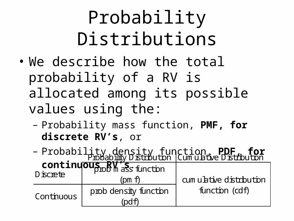
• We describe how the total probability of a RV is allocated among its possible values using the:– Probability mass function, PMF, for discrete

RV’s, or– Probability density function, PDF, for

continuous RV’s. Probability Distribution Cumulative Distribution

Discreteprob mass function

(pmf)

Continuousprob density function

(pdf)

cumulative distribution function (cdf)

II. Probability distributions for discrete random

variables

1 and 0 :subject to

:

xpxp

xsXSsPxXPxp

Re-stated: for every possible value x of the random variable, the PMF specifies the probability of observing that value.

The PMF, p(x), of a discrete R.V. is defined for every number x by:

Exercise 2: PMF

• The sample space of a random experiment is {a,b,c,d,e,f}, and each outcome is equally likely. A rv X is defined as follows:

Determine the pmf of Xp(0) p( ) p( )

Outcome a b c d e fx 0 0 1 1 2 3

Exercise 3

• Consider a group of five potential blood donors {A,B,C,D,E}. Only A and B have type O+.

• Suppose you take five blood samples, one from each individual, in random order. If RV Y = # of samples necessary to identify an O+ individual, define the PMF of Y.

Family of Probability Distributions

• When p(x) depends on a parameter, the collection of all probability distributions for different values of the parameter is called a family of probability distributions.

Probability Family Example

• The probability mass function of any Bernoulli random variable can be expressed in terms of a single parameter:

otherwise 0

1 if

0 if 1

;

:as expressedoften also isIt

10 where10 1

x

x

xp

pp

Cumulative Distribution Function

• The cumulative distribution function (CDF) F(x) of a discrete random variable X is defined by:

• Example: Determine the CDF for Y if its probability mass function is given by:

xyy

ypxXPxF:

y 1 2 3 4p(y) 0.4 0.3 0.2 0.1

Exercise 4

• We may derive the PMF from the CDF:– Suppose that X is the number of sick days

taken by an employee. If the maximum number is 14, possible values range from 0 to 14. If

52

)3(

3

94.05,88.04

81.03,76.02,72.01,58.00

XP

XP

XP

FF

FFFF

III. Expected values of discrete random variables

• The expected value or mean value of a discrete random variable X can be defined as:

Where X can take values from the set D

Dx

X xpxXE

Exercise 5

• Let X be a discrete RV that equals the number of bits in error during a digital transmission. Suppose X can take values from 0 to 4. The PMF is defined as follows:

x 0 1 2 3 4p(x) 0.6561 0.2916 0.0486 0.0036 0.0001

?XE

Expected Value of a Function of a Random

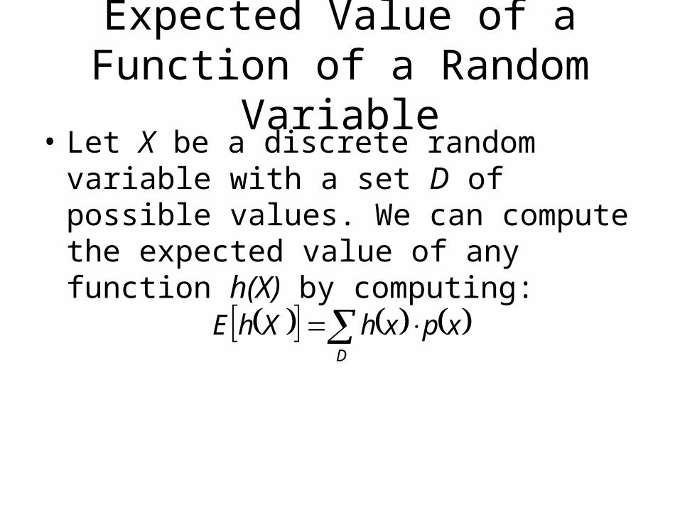
Variable• Let X be a discrete random variable

with a set D of possible values. We can compute the expected value of any function h(X) by computing:

xpxhXhED

Exercise 6

• Let X = the outcome when a fair die is rolled once.

• A gambler offers you the following 2 different options:– Do not roll the die and be paid nothing, or

– Roll the die and be paid h(X)=$(1/X - 1/3.5) , where X is the outcome of rolling the die once.

• Should you roll the die?

Rules of Expected Value

• E(X) is a “Linear Operator”, i.e.;–

–

XEaxpxaxpaxaXE

XEaaXE

bXEbXE

xpbxpxxpbxbXE

bXEbXE

Exercise 7

• Use the rules for expected values to calculate:

?

?

XE

cXE

Variance of x

• The variance of a discrete RV X, V(X), is:

2

22222

222

:is of (SD)deviation standard The

:is Formulashortcut A

XX

DX

DX

X

XEXExpxXV

XExpxXV

Rules of Variance

• Two important rules of Variance:

• Variance of a function h(X):

XbX

XaX

XVbXV

aXVaaXV

2

xpXhEXhXhVD

2

Exercise 8

• A computer store purchases 3 computers at $500 a piece. The computers will be sold at a price of $1000. The manufacturer will re-purchase any unsold computers from the computer store after a time period for $200 a piece. Let X be the # of computers sold at the end of the period.

?

?

profitV

profitEx 0 1 2 3p(x) 0.1 0.2 0.3 0.4