1 INTERPRETATION OF A REGRESSION EQUATION The scatter diagram shows hourly earnings in 1994 plotted...

1

INTERPRETATION OF A REGRESSION EQUATION

The scatter diagram shows hourly earnings in 1994 plotted against highest grade completed for a sample of 570 respondents.

-10

0

10

20

30

40

50

60

70

80

0 1 2 3 4 5 6 7 8 9 10 11 12 13 14 15 16 17 18 19 20

Years of schooling

Ho

url

y e

arn

ing

s ($

)

. reg EARNINGS S

Source | SS df MS Number of obs = 570---------+------------------------------ F( 1, 568) = 65.64 Model | 3977.38016 1 3977.38016 Prob > F = 0.0000Residual | 34419.6569 568 60.5979875 R-squared = 0.1036---------+------------------------------ Adj R-squared = 0.1020 Total | 38397.0371 569 67.4816117 Root MSE = 7.7845

------------------------------------------------------------------------------EARNINGS | Coef. Std. Err. t P>|t| [95% Conf. Interval]---------+-------------------------------------------------------------------- S | 1.073055 .1324501 8.102 0.000 .8129028 1.333206 _cons | -1.391004 1.820305 -0.764 0.445 -4.966354 2.184347------------------------------------------------------------------------------


This is the output from a regression of earnings on highest grade completed, using Stata.

4

SEARNINGS 07313911 ..

. reg EARNINGS S




For the time being, we will be concerned only with the estimates of the parameters. The variables in the regression are listed in the first column and the second column gives the estimates of their coefficients.

5


. reg EARNINGS S




In this case there is only one variable, S, and its coefficient is 1.073. _cons, in Stata, refers to the constant. The estimate of the intercept is -1.391.

6


-10

0

10

20

30

40

50

60

70

80

0 1 2 3 4 5 6 7 8 9 10 11 12 13 14 15 16 17 18 19 20

Years of schooling

Ho

url

y e

arn

ing

s ($

)

7

Here is the scatter diagram again, with the regression line shown.


SEARNINGS 07313911 .. ^

-10

0

10

20

30

40

50

60

70

80

0 1 2 3 4 5 6 7 8 9 10 11 12 13 14 15 16 17 18 19 20

Years of schooling

Ho

url

y e

arn

ing

s ($

)


SEARNINGS 07313911 .. ^

What do the coefficients actually mean?

8

-10

0

10

20

30

40

50

60

70

80

0 1 2 3 4 5 6 7 8 9 10 11 12 13 14 15 16 17 18 19 20

Years of schooling

Ho

url

y e

arn

ing

s ($

)


SEARNINGS 07313911 .. ^

To answer this question, you must refer to the units in which the variables are measured.

9

-10

0

10

20

30

40

50

60

70

80

0 1 2 3 4 5 6 7 8 9 10 11 12 13 14 15 16 17 18 19 20

Years of schooling

Ho

url

y e

arn

ing

s ($

)


SEARNINGS 07313911 .. ^

S is measured in years (strictly speaking, grades completed), EARNINGS in dollars per hour. So the slope coefficient implies that hourly earnings increase by $1.07 for each extra year of schooling.

10

-10

0

10

20

30

40

50

60

70

80

0 1 2 3 4 5 6 7 8 9 10 11 12 13 14 15 16 17 18 19 20

Years of schooling

Ho

url

y e

arn

ing

s ($

)

11

We will look at a geometrical representation of this interpretation. To do this, we will enlarge the marked section of the scatter diagram.


SEARNINGS 07313911 .. ^

7

8

9

10

11

12

13

14

15

10.8 11 11.2 11.4 11.6 11.8 12 12.2

Highest grade completed

Ho

url

y ea

rnin

gs

($)

The regression line indicates that completing 12th grade instead of 11th grade would increase earnings by $1.073, from $10.413 to $11.486, as a general tendency.


12

One year

$1.07

$10.41

$11.49

-10

0

10

20

30

40

50

60

70

80

0 1 2 3 4 5 6 7 8 9 10 11 12 13 14 15 16 17 18 19 20

Years of schooling

Ho

url

y e

arn

ing

s ($

)

13

You should ask yourself whether this is a plausible figure. If it is implausible, this could be a sign that your model is misspecified in some way.


^SEARNINGS 07313911 ..

-10

0

10

20

30

40

50

60

70

80

0 1 2 3 4 5 6 7 8 9 10 11 12 13 14 15 16 17 18 19 20

Years of schooling

Ho

url

y e

arn

ing

s ($

)

14

For low levels of education it might be plausible. But for high levels it would seem to be an underestimate.



-10

0

10

20

30

40

50

60

70

80

0 1 2 3 4 5 6 7 8 9 10 11 12 13 14 15 16 17 18 19 20

Years of schooling

Ho

url

y e

arn

ing

s ($

)

15

What about the constant term? (Try to answer this question yourself before continuing with this sequence.)



-10

0

10

20

30

40

50

60

70

80

0 1 2 3 4 5 6 7 8 9 10 11 12 13 14 15 16 17 18 19 20

Years of schooling

Ho

url

y e

arn

ing

s ($

)

16

Literally, the constant indicates that an individual with no years of education would have to pay $1.39 per hour to be allowed to work.



-10

0

10

20

30

40

50

60

70

80

0 1 2 3 4 5 6 7 8 9 10 11 12 13 14 15 16 17 18 19 20

Years of schooling

Ho

url

y e

arn

ing

s ($

)

17

This does not make any sense at all, an interpretation of negative payment is impossible to sustain.



-10

0

10

20

30

40

50

60

70

80

0 1 2 3 4 5 6 7 8 9 10 11 12 13 14 15 16 17 18 19 20

Years of schooling

Ho

url

y e

arn

ing

s ($

)

18

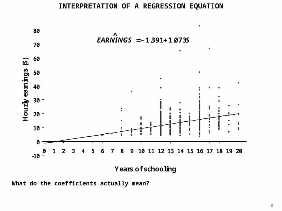
A safe solution to the problem is to limit the interpretation to the range of the sample data, and to refuse to extrapolate on the ground that we have no evidence outside the data range.



19

With this explanation, the only function of the constant term is to enable you to draw the regression line at the correct height on the scatter diagram. It has no meaning of its own.



-10

0

10

20

30

40

50

60

70

80

0 1 2 3 4 5 6 7 8 9 10 11 12 13 14 15 16 17 18 19 20

Years of schooling

Ho

url

y e

arn

ing

s ($

)

MULTIPLE REGRESSION WITH TWO EXPLANATORY VARIABLES: EXAMPLE

EARNINGS = 1 + 2S + 3A+ u

2

Specifically, we will look at an earnings function model where hourly earnings, EARNINGS, depend on years of schooling (highest grade completed), S, and a measure of cognitive ability, A.

The model has three dimensions, one each for EARNINGS, S, and A. The starting point for

investigating the determination of EARNINGS is the intercept, 1.

Literally the intercept gives EARNINGS for those respondents who have no schooling and who scored zero on the ability test. However, the ability score is scaled in such a way as to

make it impossible to score zero. Hence a literal interpretation of 1 would be unwise.

The next term on the right side of the equation gives the effect of variations in S. A one

year increase in S causes EARNINGS to increase by 2 dollars, holding A constant.

Similarly, the third term gives the effect of variations in A. A one point increase in A causes

earnings to increase by 3 dollars, holding S constant.

The final element of the model is the disturbance term, u. In this observation, u happens to have a positive value.

iiii uXXY 33221

iii XbXbbY 33221ˆ


The regression coefficients are derived using the same least squares principle used in simple regression analysis. The fitted value of Y in observation i depends on our choice of b1, b2, and b3.

11

A sample consists of a number of observations generated in this way. Note that the interpretation of the model does not depend on whether S and A are correlated or not.

However we do assume that the effects of S and A on EARNINGS are additive. The impact of a difference in S on EARNINGS is not affected by the value of A, or vice versa.

iiii uXXY 33221

iii XbXbbY 33221ˆ

iiiiii XbXbbYYYe 33221ˆ


The residual ei in observation i is the difference between the actual and fitted values of Y.

12

233221

2 )( iiii XbXbbYeRSS


We define RSS, the sum of the squares of the residuals, and choose b1, b2, and b3 so as to minimize it.

13

. reg EARNINGS S ASVABC


------------------------------------------------------------------------------EARNINGS | Coef. Std. Err. t P>|t| [95% Conf. Interval]---------+-------------------------------------------------------------------- S | .7390366 .1606216 4.601 0.000 .4235506 1.054523 ASVABC | .1545341 .0429486 3.598 0.000 .0701764 .2388918 _cons | -4.624749 2.0132 -2.297 0.022 -8.578989 -.6705095------------------------------------------------------------------------------


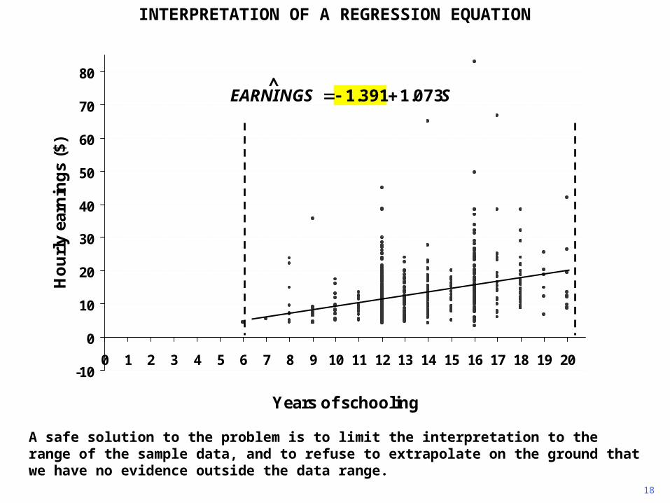
Here is the regression output for the earnings function using Data Set 21.

19

ASVABCSINGSNEAR 15.074.062.4ˆ

. reg EARNINGS S A


------------------------------------------------------------------------------EARNINGS | Coef. Std. Err. t P>|t| [95% Conf. Interval]---------+-------------------------------------------------------------------- S | .7390366 .1606216 4.601 0.000 .4235506 1.054523 A | .1545341 .0429486 3.598 0.000 .0701764 .2388918 _cons | -4.624749 2.0132 -2.297 0.022 -8.578989 -.6705095------------------------------------------------------------------------------


20

It indicates that earnings increase by $0.74 for every extra year of schooling and by $0.15 for every extra point increase in A.

ASINGSNEAR 15.074.062.4ˆ

. reg EARNINGS S A




21

Literally, the intercept indicates that an individual who had no schooling and an A score of zero would have hourly earnings of -$4.62.


. reg EARNINGS S A




22

Obviously, this is impossible. The lowest value of S in the sample was 6, and the lowest A score was 22. We have obtained a nonsense estimate because we have extrapolated too far from the data range.


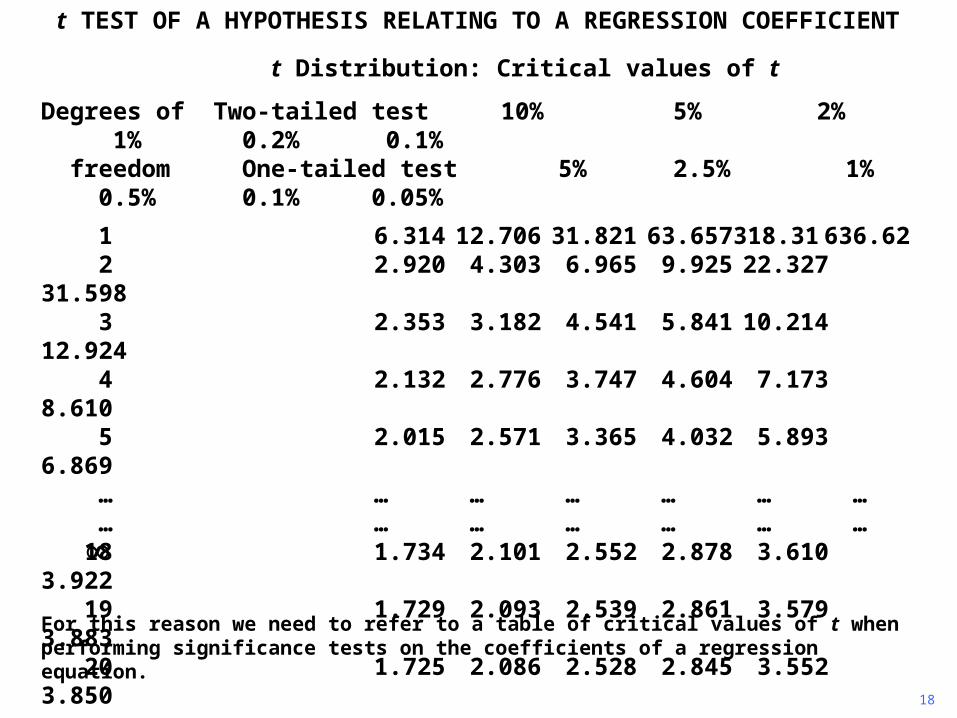
t Distribution: Critical values of t

Degrees of Two-tailed test 10% 5% 2% 1% 0.2% 0.1% freedom One-tailed test 5% 2.5% 1% 0.5% 0.1% 0.05%

1 6.314 12.706 31.821 63.657 318.31 636.622 2.920 4.303 6.965 9.925 22.327 31.5983 2.353 3.182 4.541 5.841 10.214 12.9244 2.132 2.776 3.747 4.604 7.173 8.6105 2.015 2.571 3.365 4.032 5.893 6.869

… … … … … … …… … … … … … …18 1.734 2.101 2.552 2.878 3.610 3.92219 1.729 2.093 2.539 2.861 3.579 3.88320 1.725 2.086 2.528 2.845 3.552 3.850… … … … … … …… … … … … … …

120 1.658 1.980 2.358 2.617 3.160 3.3731.645 1.960 2.326 2.576 3.090 3.291

18

t TEST OF A HYPOTHESIS RELATING TO A REGRESSION COEFFICIENT

For this reason we need to refer to a table of critical values of t when performing significance tests on the coefficients of a regression equation.



1 6.314 12.706 31.821 63.657 318.31 636.622 2.920 4.303 6.965 9.925 22.327 31.5983 2.353 3.182 4.541 5.841 10.214 12.9244 2.132 2.776 3.747 4.604 7.173 8.6105 2.015 2.571 3.365 4.032 5.893 6.869

… … … … … … …… … … … … … …18 1.734 2.101 2.552 2.878 3.610 3.92219 1.729 2.093 2.539 2.861 3.579 3.88320 1.725 2.086 2.528 2.845 3.552 3.850… … … … … … …… … … … … … …

120 1.658 1.980 2.358 2.617 3.160 3.3731.645 1.960 2.326 2.576 3.090 3.291

19


At the top of the table are listed possible significance levels for a test. For the time being we will be performing two-tailed tests, so ignore the line for one-tailed tests.



1 6.314 12.706 31.821 63.657 318.31 636.622 2.920 4.303 6.965 9.925 22.327 31.5983 2.353 3.182 4.541 5.841 10.214 12.9244 2.132 2.776 3.747 4.604 7.173 8.6105 2.015 2.571 3.365 4.032 5.893 6.869

… … … … … … …… … … … … … …18 1.734 2.101 2.552 2.878 3.610 3.92219 1.729 2.093 2.539 2.861 3.579 3.88320 1.725 2.086 2.528 2.845 3.552 3.850… … … … … … …… … … … … … …

120 1.658 1.980 2.358 2.617 3.160 3.3731.645 1.960 2.326 2.576 3.090 3.291

20


Hence if we are performing a (two-tailed) 5% significance test, we should use the column thus indicated in the table.



1 6.314 12.706 31.821 63.657 318.31 636.622 2.920 4.303 6.965 9.925 22.327 31.5983 2.353 3.182 4.541 5.841 10.214 12.9244 2.132 2.776 3.747 4.604 7.173 8.6105 2.015 2.571 3.365 4.032 5.893 6.869

… … … … … … …… … … … … … …18 1.734 2.101 2.552 2.878 3.610 3.92219 1.729 2.093 2.539 2.861 3.579 3.88320 1.725 2.086 2.528 2.845 3.552 3.850… … … … … … …… … … … … … …

120 1.658 1.980 2.358 2.617 3.160 3.3731.645 1.960 2.326 2.576 3.090 3.291

21


The left hand vertical column lists degrees of freedom. The number of degrees of freedom in a regression is defined to be the number of observations minus the number of parameters estimated.

Number of degrees of freedom in a regression

= number of observations - number of parameters estimated.



1 6.314 12.706 31.821 63.657 318.31 636.622 2.920 4.303 6.965 9.925 22.327 31.5983 2.353 3.182 4.541 5.841 10.214 12.9244 2.132 2.776 3.747 4.604 7.173 8.6105 2.015 2.571 3.365 4.032 5.893 6.869

… … … … … … …… … … … … … …18 1.734 2.101 2.552 2.878 3.610 3.92219 1.729 2.093 2.539 2.861 3.579 3.88320 1.725 2.086 2.528 2.845 3.552 3.850… … … … … … …… … … … … … …

120 1.658 1.980 2.358 2.617 3.160 3.3731.645 1.960 2.326 2.576 3.090 3.291

22


In a simple regression, we estimate just two parameters, the constant and the slope coefficient, so the number of degrees of freedom is n - 2 if there are n observations.



1 6.314 12.706 31.821 63.657 318.31 636.622 2.920 4.303 6.965 9.925 22.327 31.5983 2.353 3.182 4.541 5.841 10.214 12.9244 2.132 2.776 3.747 4.604 7.173 8.6105 2.015 2.571 3.365 4.032 5.893 6.869

… … … … … … …… … … … … … …18 1.734 2.101 2.552 2.878 3.610 3.92219 1.729 2.093 2.539 2.861 3.579 3.88320 1.725 2.086 2.528 2.845 3.552 3.850… … … … … … …… … … … … … …

120 1.658 1.980 2.358 2.617 3.160 3.3731.645 1.960 2.326 2.576 3.090 3.291

23


If we were performing a regression with 20 observations, as in the price inflation/wage inflation example, the number of degrees of freedom would be 18 and the critical value of t for a 5% test would be 2.101.



1 6.314 12.706 31.821 63.657 318.31 636.622 2.920 4.303 6.965 9.925 22.327 31.5983 2.353 3.182 4.541 5.841 10.214 12.9244 2.132 2.776 3.747 4.604 7.173 8.6105 2.015 2.571 3.365 4.032 5.893 6.869

… … … … … … …… … … … … … …18 1.734 2.101 2.552 2.878 3.610 3.92219 1.729 2.093 2.539 2.861 3.579 3.88320 1.725 2.086 2.528 2.845 3.552 3.850… … … … … … …… … … … … … …

120 1.658 1.980 2.358 2.617 3.160 3.3731.645 1.960 2.326 2.576 3.090 3.291

24


Note that as the number of degrees of freedom becomes large, the critical value converges on 1.96, the critical value for the normal distribution. This is because the t distribution converges on the normal distribution.



1 6.314 12.706 31.821 63.657 318.31 636.622 2.920 4.303 6.965 9.925 22.327 31.5983 2.353 3.182 4.541 5.841 10.214 12.9244 2.132 2.776 3.747 4.604 7.173 8.6105 2.015 2.571 3.365 4.032 5.893 6.869

… … … … … … …… … … … … … …18 1.734 2.101 2.552 2.878 3.610 3.92219 1.729 2.093 2.539 2.861 3.579 3.88320 1.725 2.086 2.528 2.845 3.552 3.850… … … … … … …… … … … … … …

120 1.658 1.980 2.358 2.617 3.160 3.3731.645 1.960 2.326 2.576 3.090 3.291

27


If instead we wished to perform a 1% significance test, we would use the column indicated above. Note that as the number of degrees of freedom becomes large, the critical value converges to 2.58, the critical value for the normal distribution.



1 6.314 12.706 31.821 63.657 318.31 636.622 2.920 4.303 6.965 9.925 22.327 31.5983 2.353 3.182 4.541 5.841 10.214 12.9244 2.132 2.776 3.747 4.604 7.173 8.6105 2.015 2.571 3.365 4.032 5.893 6.869

… … … … … … …… … … … … … …18 1.734 2.101 2.552 2.878 3.610 3.92219 1.729 2.093 2.539 2.861 3.579 3.88320 1.725 2.086 2.528 2.845 3.552 3.850… … … … … … …… … … … … … …

120 1.658 1.980 2.358 2.617 3.160 3.3731.645 1.960 2.326 2.576 3.090 3.291

28


For a simple regression with 20 observations, the critical value of t at the 1% level is 2.878.


s.d. of b2 known

discrepancy between hypothetical value and sample estimate, in terms of s.d.:

s.d.

022

b

z

5% significance test:

reject H0: 2 = 2 if

z > 1.96 or z < -1.96

s.d. of b2 not known

discrepancy between hypothetical value and sample estimate, in terms of s.e.:

s.e.

022

b

t

1% significance test:

reject H0: 2 = 2 if

t > 2.878 or t < -2.878

0 0

So we should this figure in the test procedure for a 1% test.

29

3.10 A researcher with a sample of 50 individuals with similar education but differing amounts of training hypothesizes that hourly earnings, EARNINGS, may be related to hours of training, TRAINING, according to the relationship

EARNINGS = 1 + 2TRAINING + u

He is prepared to test the null hypothesis H0: 2 = 0 against the alternative hypothesis H1: 2 0 at the 5 percent and 1 percent levels. What should he report

1. If b2 = 0.30, s.e.(b2) = 0.12? 2. If b2 = 0.55, s.e.(b2) = 0.12? 3. If b2 = 0.10, s.e.(b2) = 0.12? 4. If b2 = -0.27, s.e.(b2) = 0.12?

EXERCISE

1


H0: 2 = 0, H1: 2 0

n = 50, so 48 degrees of freedom

EXERCISE

There are 50 observations and 2 parameters have been estimated, so there are 48 degrees of freedom.

2


H0: 2 = 0, H1: 2 0


tcrit, 5% = 2.01, tcrit, 1% = 2.68

EXERCISE

The table giving the critical values of t does not give the values for 48 degrees of freedom. We will use the values for 50 as a guide. For the 5% level the value is 2.01, and for the 1% level it is 2.68. The critical values for 48 will be slightly higher.

3


H0: 2 = 0, H1: 2 0


tcrit, 5% = 2.01, tcrit, 1% = 2.68_______________________________________________

1. If b2 = 0.30, s.e.(b2) = 0.12?

t = 2.50.

EXERCISE

In the first case, the t statistic is 2.50.

4


H0: 2 = 0, H1: 2 0


tcrit, 5% = 2.01, tcrit, 1% = 2.68_______________________________________________

1. If b2 = 0.30, s.e.(b2) = 0.12?

t = 2.50. Reject H0 at the 5% level but not at the 1%

level.

EXERCISE

5

This is greater than the critical value of t at the 5% level, but less than the critical value at the 1% level.


H0: 2 = 0, H1: 2 0


tcrit, 5% = 2.01, tcrit, 1% = 2.68_______________________________________________

1. If b2 = 0.30, s.e.(b2) = 0.12?

t = 2.50. Reject H0 at the 5%, but not at the 1%, level.

EXERCISE

In this case we should mention both tests. It is not enough to say "Reject at the 5% level", because it leaves open the possibility that we might be able to reject at the 1% level.

6


H0: 2 = 0, H1: 2 0


tcrit, 5% = 2.01, tcrit, 1% = 2.68_______________________________________________

1. If b2 = 0.30, s.e.(b2) = 0.12?

t = 2.50. Reject H0 at the 5%, but not at the 1%, level.

EXERCISE

Likewise it is not enough to say "Do not reject at the 1% level", because this does not reveal whether the result is significant at the 5% level or not.

7


H0: 2 = 0, H1: 2 0


tcrit, 5% = 2.01, tcrit, 1% = 2.68_______________________________________________

2. If b2 = 0.55, s.e.(b2) = 0.12?

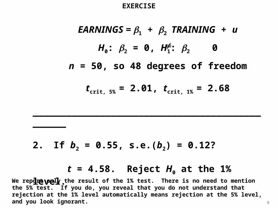
t = 4.58.

EXERCISE

In the second case, t is equal to 4.58.

8


H0: 2 = 0, H1: 2 0


tcrit, 5% = 2.01, tcrit, 1% = 2.68_______________________________________________

2. If b2 = 0.55, s.e.(b2) = 0.12?

t = 4.58. Reject H0 at the 1% level.

EXERCISE

We report only the result of the 1% test. There is no need to mention the 5% test. If you do, you reveal that you do not understand that rejection at the 1% level automatically means rejection at the 5% level, and you look ignorant.

9


H0: 2 = 0, H1: 2 0


tcrit, 5% = 2.01, tcrit, 1% = 2.68_______________________________________________

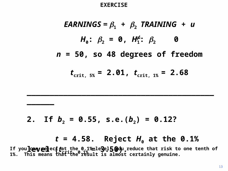
2. If b2 = 0.55, s.e.(b2) = 0.12?

t = 4.58. Reject H0 at the 0.1% level (tcrit, 0.1% = 3.50).

EXERCISE

Actually, given the large t statistic, it is a good idea to investigate whether we can reject H0 at the 0.1% level. It turns out that we can. The critical value for 50 degrees of freedom is 3.50. So we just report the outcome of this test. There is no need to mention the 1% test.

10


H0: 2 = 0, H1: 2 0


tcrit, 5% = 2.01, tcrit, 1% = 2.68_______________________________________________

2. If b2 = 0.55, s.e.(b2) = 0.12?


EXERCISE

Why is it a good idea to press on to a 0.1% test, if the t statistic is large? Try to answer this question before looking at the next slide.

11


H0: 2 = 0, H1: 2 0


tcrit, 5% = 2.01, tcrit, 1% = 2.68_______________________________________________

2. If b2 = 0.55, s.e.(b2) = 0.12?


EXERCISE 3.10

The reason is that rejection at the 1% level still leaves open the possibility of a 1% risk of having made a Type I error (rejecting the null hypothesis when it is in fact true). So there is a 1% risk of the "significant" result having occurred as a matter of chance.

12


H0: 2 = 0, H1: 2 0


tcrit, 5% = 2.01, tcrit, 1% = 2.68_______________________________________________

2. If b2 = 0.55, s.e.(b2) = 0.12?


EXERCISE

13

If you can reject at the 0.1% level, you reduce that risk to one tenth of 1%. This means that the result is almost certainly genuine.


H0: 2 = 0, H1: 2 0


tcrit, 5% = 2.01, tcrit, 1% = 2.68_______________________________________________

3. If b2 = 0.10, s.e.(b2) = 0.12?

t = 0.83.

EXERCISE

14

In the third case, t is equal to 0.83.


H0: 2 = 0, H1: 2 0


tcrit, 5% = 2.01, tcrit, 1% = 2.68_______________________________________________

3. If b2 = 0.10, s.e.(b2) = 0.12?

t = 0.83. Do not reject H0 at the 5% level.

EXERCISE

15

We report only the result of the 5% test. There is no need to mention the 1% test. If you do, you reveal that you do not understand that not rejecting at the 5% level automatically means not rejecting at the 1% level, and you look ignorant.


H0: 2 = 0, H1: 2 0


tcrit, 5% = 2.01, tcrit, 1% = 2.68_______________________________________________

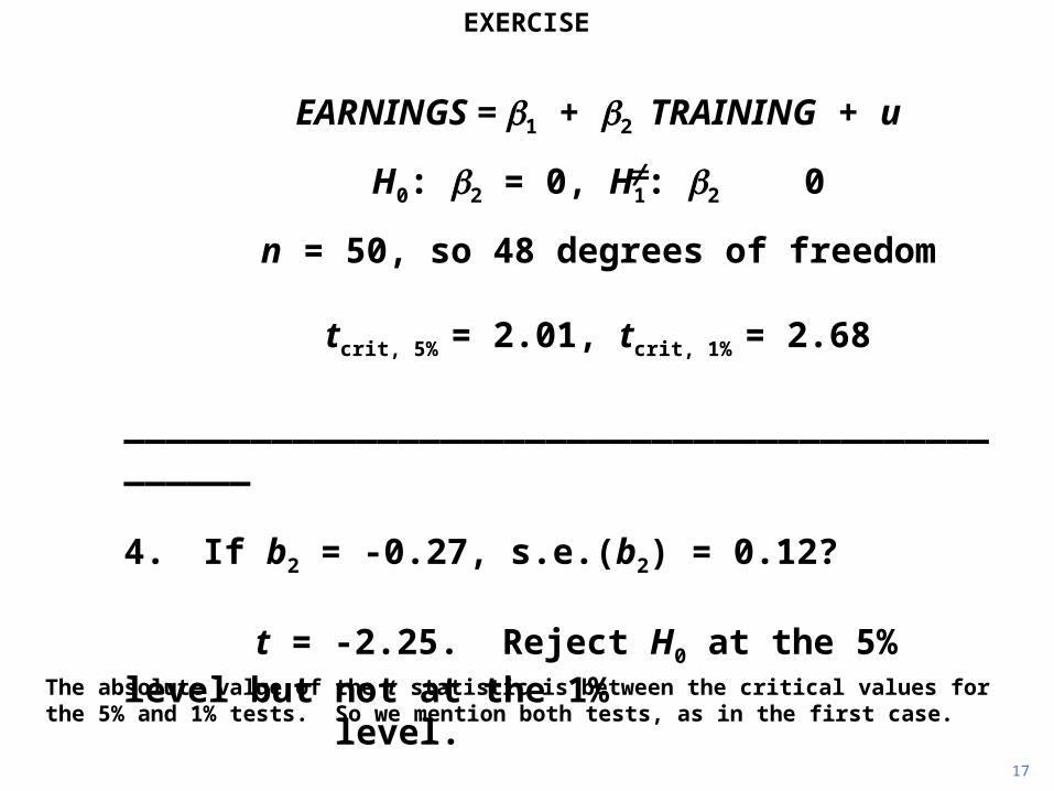
4. If b2 = -0.27, s.e.(b2) = 0.12?

t = -2.25.

EXERCISE

In the fourth case, t is equal to -2.25.

16


H0: 2 = 0, H1: 2 0


tcrit, 5% = 2.01, tcrit, 1% = 2.68_______________________________________________

4. If b2 = -0.27, s.e.(b2) = 0.12?

t = -2.25. Reject H0 at the 5% level but not at the 1% level.

EXERCISE

The absolute value of the t statistic is between the critical values for the 5% and 1% tests. So we mention both tests, as in the first case.

17

F TESTS OF GOODNESS OF FIT

1

This sequence describes two F tests of goodness of fit in a multiple regression model. The first relates to the goodness of fit of the equation as a whole.

uXXY kk ...221

0 oneleast at :

0...:

1

20

H

H k


2

We will consider the general case where there are k - 1 explanatory variables. For the F test of goodness of fit of the equation as a whole, the null hypothesis, in words, is that the model has no explanatory power at all.

uXXY kk ...221

0 oneleast at :

0...:

1

20

H

H k


3

Of course we hope to reject it and conclude that the model does have some explanatory power.

uXXY kk ...221

0 oneleast at :

0...:

1

20

H

H k


4

The model will have no explanatory power if it turns out that Y is unrelated to any of the explanatory variables. Mathematically, therefore, the null hypothesis is that all the

coefficients 2, ..., k are zero.

uXXY kk ...221

0 oneleast at :

0...:

1

20

H

H k


uXXY kk ...221

0 oneleast at :

0...:

1

20

H

H k

5

The alternative hypothesis is that at least one of these coefficients is different from zero.


uXXY kk ...221

0 oneleast at :

0...:

1

20

H

H k

6

In the multiple regression model there is a difference between the roles of the F and t tests. The F test tests the joint explanatory power of the variables, while the t tests test their explanatory power individually.


uXXY kk ...221

0 oneleast at :

0...:

1

20

H

H k

7

In the simple regression model the F test was equivalent to the (two-tailed) t test on the slope coefficient because the "group" consisted of just one variable.


)()1()1(

)(

)1(

)()1(

),1(

2

2

knRkR

knTSSRSS

kTSSESS

knRSSkESS

knkF

uXXY kk ...221

0 oneleast at :

0...:

1

20

H

H k

8

The F statistic for the test was defined in the last sequence in Chapter 3. ESS is the explained sum of squares and RSS is the residual sum of squares.


)()1()1(

)(

)1(

)()1(

),1(

2

2

knRkR

knTSSRSS

kTSSESS

knRSSkESS

knkF

uXXY kk ...221

0 oneleast at :

0...:

1

20

H

H k

9

It can be expressed in terms of R2 by dividing the numerator and denominator by TSS, the total sum of squares.


10

)()1()1(

)(

)1(

)()1(

),1(

2

2

knRkR

knTSSRSS

kTSSESS

knRSSkESS

knkF

uXXY kk ...221

0 oneleast at :

0...:

1

20

H

H k

ESS / TSS is equal to R2 and RSS / TSS is equal to (1 - R2). (For proofs, see the last sequence in Chapter 3.)


11

uSFSMASVABCS 4321

The educational attainment model will be used as an example. We will suppose that S depends on ASVABC, the ability score, and SM, and SF, the highest grade completed by the mother and father of the respondent, respectively.


12

0: 4320 H

The null hypothesis for the F test of goodness of fit is that all three slope coefficients are equal to zero. The alternative hypothesis is that at least one of them is non-zero.

uSFSMASVABCS 4321

. reg S ASVABC SM SF


------------------------------------------------------------------------------ S | Coef. Std. Err. t P>|t| [95% Conf. Interval]---------+-------------------------------------------------------------------- ASVABC | .1295006 .0099544 13.009 0.000 .1099486 .1490527 SM | .069403 .0422974 1.641 0.101 -.013676 .152482 SF | .1102684 .0311948 3.535 0.000 .0489967 .1715401 _cons | 4.914654 .5063527 9.706 0.000 3.920094 5.909214------------------------------------------------------------------------------


13

Here is the regression output using Data Set 21.

uSFSMASVABCS 4321 0: 4320 H






14

)/()1/(

),1(knRSS

kESSknkF

In this example, k - 1, the number of explanatory variables, is equal to 3 and n - k, the number of degrees of freedom, is equal to 566.

8.110566/21763/1278

)566,3( F






)/()1/(

),1(knRSS

kESSknkF

8.110

566/21763/1278

)566,3( F

15

The numerator of the F statistic is the explained sum of squares divided by k - 1. In the Stata output these numbers are given in the Model row.






)/()1/(

),1(knRSS

kESSknkF

8.110

566/21763/1278

)566,3( F

16

The denominator is the residual sum of squares divided by the number of degrees of freedom remaining.






)/()1/(

),1(knRSS

kESSknkF

8.110

566/21763/1278

)566,3( F

17

Hence the F statistic is 110.8. All serious regression packages compute it for you as part of the diagnostics in the regression output.






8.110566/21763/1278

)566,3( F

18

The critical value for F(3,566) is not given in the F tables, but we know it must be lower than F(3,120), which is given. At the 0.1% level, this is 5.78. Hence we easily reject H0 at the 0.1% level.

78.5)120,3(crit,0.1% F






8.110566/21763/1278

)566,3( F78.5)120,3(crit,0.1% F

19

This result could have been anticipated because both ASVABC and SF have highly

significant t statistics. So we knew in advance that both 2 and 4 were non-zero.






8.110566/21763/1278

)566,3( F78.5)120,3(crit,0.1% F

20

It is unusual for the F statistic not to be significant if some of the t statistics are significant. In principle it could happen though. Suppose that you ran a regression with 40 explanatory variables, none being a true determinant of the dependent variable.






8.110566/21763/1278

)566,3( F78.5)120,3(crit,0.1% F

21

Then the F statistic should be low enough for H0 not to be rejected. However, if you are performing t tests on the slope coefficients at the 5% level, with a 5% chance of a Type I error, on average 2 of the 40 variables could be expected to have "significant" coefficients.






8.110566/21763/1278

)566,3( F78.5)120,3(crit,0.1% F

22

The opposite can easily happen, though. Suppose you have a multiple regression model which is correctly specified and the R2 is high. You would expect to have a highly significant F statistic.






8.110566/21763/1278

)566,3( F78.5)120,3(crit,0.1% F

23

However, if the explanatory variables are highly correlated and the model is subject to severe multicollinearity, the standard errors of the slope coefficients could all be so large that none of the t statistics is significant.

1 INTERPRETATION OF A REGRESSION EQUATION The scatter diagram shows hourly earnings in 1994 plotted...

Documents

Transcript of 1 INTERPRETATION OF A REGRESSION EQUATION The scatter diagram shows hourly earnings in 1994 plotted...