
1-Dimensional Simulation of Thermal Annealing in a ...
167
SAND94-0135 Distribution Unlimited Release Category UC-523 Printed November 1994 1-Dimensional Simulation of Thermal Annealing in a Commercial Nuclear Power Plant Reactor Pressure Vessel Wall Section FINAL REPORT Prepared by: James T. Nakos and Stan T. Rosinski DOE's Light Water Reactor Technology Center Advanced Nuclear Power Technology Department 6471 Sandia National Laboratories Russell U. Acton Thermal Test Team Energetic & Environmental Test Department 2761 Sandia National Laboratories Abstract The objective of this work was to provide experimental heat transfer boundary condition and reactor pressure vessel (RPV) section thermal response data that can be used to benchmark computer codes that simulate thermal annealing of RPVs. This specific project was designed to provide the Electric Power Research Institute (EPRI) with experimental data that could be used to support the development of a thermal annealing model. A secondary benefit is to provide additional experimental data (e.g., thermal response of concrete reactor cavity wall) that could be of use in an annealing demonstration project. The setup comprised a heater assembly, a 1.2 m x 1.2 m x 17.1 cm thick [4 ft x 4 ft x 6.75 in] section of an RPV (A533B ferritic steel with stainless steel cladding), a mockup of the "mirror" insulation between the RPV and the concrete reactor cavity wall, and a 25.4 cm [10 in] thick concrete wall, 2.1 m x 2.1 m [10 ft x 10 ft] square. Experiments were performed at temperature heat-up/cooldown rates of 7, 14, and 28°C/hr [12.5, 25, and 50°F/hr] as measured on the heated face. A peak temperature of 454°C [850°F] was maintained on the heated face until the concrete wall temperature reached equilibrium. Results are most representative of those RPV locations where the heat transfer would be 1-dimensional. Temperature was measured at multiple locations on the heated and unheated faces of the RPV section and the concrete wall. Incident heat flux was measured on the heated face, and absorbed heat flux estimates were generated from temperature measurements and an inverse heat conduction code developed at Sandia National Laboratories called "Sandia One Dimensional Direct and Inverse Thermal" (SODDIT). Through-wall temperature differences, concrete wall temperature response, heat flux absorbed into the RPV surface and incident on the surface are presented. All of these data are useful to modelers developing codes to simulate RPV annealing. Additionally, incident heat flux measurements can be used to design the heater system required to anneal a full-scale RPV. Results compare favorably with those reported in NUREG/CR-4212. DISTRIBUTION OF THIS DOCUMENT IS UNLIMITED
Transcript of 1-Dimensional Simulation of Thermal Annealing in a ...
SAND94-0135 Distribution Unlimited Release Category UC-523
Printed November 1994
1-Dimensional Simulation of Thermal Annealing in a Commercial Nuclear Power Plant Reactor Pressure Vessel Wall Section
FINAL REPORT
Prepared by:
James T. Nakos and Stan T. Rosinski DOE's Light Water Reactor Technology Center
Advanced Nuclear Power Technology Department 6471 Sandia National Laboratories
Russell U. Acton Thermal Test Team
Energetic & Environmental Test Department 2761 Sandia National Laboratories
Abstract
The objective of this work was to provide experimental heat transfer boundary condition and reactor pressure vessel (RPV) section thermal response data that can be used to benchmark computer codes that simulate thermal annealing of RPVs. This specific project was designed to provide the Electric Power Research Institute (EPRI) with experimental data that could be used to support the development of a thermal annealing model. A secondary benefit is to provide additional experimental data (e.g., thermal response of concrete reactor cavity wall) that could be of use in an annealing demonstration project. The setup comprised a heater assembly, a 1.2 m x 1.2 m x 17.1 cm thick [4 ft x 4 ft x 6.75 in] section of an RPV (A533B ferritic steel with stainless steel cladding), a mockup of the "mirror" insulation between the RPV and the concrete reactor cavity wall, and a 25.4 cm [10 in] thick concrete wall, 2.1 m x 2.1 m [10 ft x 10 ft] square. Experiments were performed at temperature heat-up/cooldown rates of 7, 14, and 28°C/hr [12.5, 25, and 50°F/hr] as measured on the heated face. A peak temperature of 454°C [850°F] was maintained on the heated face until the concrete wall temperature reached equilibrium. Results are most representative of those RPV locations where the heat transfer would be 1-dimensional. Temperature was measured at multiple locations on the heated and unheated faces of the RPV section and the concrete wall. Incident heat flux was measured on the heated face, and absorbed heat flux estimates were generated from temperature measurements and an inverse heat conduction code developed at Sandia National Laboratories called "Sandia One Dimensional Direct and Inverse Thermal" (SODDIT). Through-wall temperature differences, concrete wall temperature response, heat flux absorbed into the RPV surface and incident on the surface are presented. All of these data are useful to modelers developing codes to simulate RPV annealing. Additionally, incident heat flux measurements can be used to design the heater system required to anneal a full-scale RPV. Results compare favorably with those reported in NUREG/CR-4212.
DISTRIBUTION OF THIS DOCUMENT IS UNLIMITED
1-Dimensional Experiments to Simulate Thermal Annealing of an RPV
Acknowledgments
This work was performed at Sandia National Laboratories (Sandia) by personnel from DOE's Light Water Reactor Technology Center. Advanced Nuclear Power Technology Department 6471 and the Thermal Test Team, Energetic & Environmental Test Department 2761. Funding and support for this work was provided by the U.S. Department of Energy, Light Water Reactor Safety & Technology Branch, NE-451, Dennis Harrison, Program Manager. The authors acknowledge the work done by members of the Thermal Test Team: Walt Gill, Bill Jacoby, Dave Schulze, and Bobby Strait. The authors would like to acknowledge the support of Larry Becker and Bob Carter from the Electric Power Research Institute's (EPRI) Non-Destructive Evaluation (NDE) Center in Charlotte. NC, who loaned the RPV section to Sandia for use in the tests and provided feedback on the draft test plan. We also acknowledge support from Rick Rishel of Westinghouse Electric Corporation, who provided input on the test plan and test setup and Tim Griesbach of ATI Consulting, Inc. (formerly of EPRI) who originally proposed the idea for the experiments.
IV

DISCLAIMER
This report was prepared as an account of work sponsored by an agency of the United States Government. Neither the United States Government nor any agency thereof, nor any of their employees, make any warranty, express or implied, or assumes any legal liability or responsibility for the accuracy, completeness, or usefulness of any information, apparatus, product, or process disclosed, or represents that its use would not infringe privately owned rights. Reference herein to any specific commercial product, process, or service by trade name, trademark, manufacturer, or otherwise does not necessarily constitute or imply its endorsement, recommendation, or favoring by the United States Government or any agency thereof. The views and opinions of authors expressed herein do not necessarily state or reflect those of the United States Government or any agency thereof.

DISCLAIMER
Portions of this document may be illegible in electronic image products. Images are produced from the best available original document.

1-Dimensional Experiments to Simulate Thermal Annealing of an RPV
Contents Figures vii
Tables xi
1. Executive Summary 1-1 1.1 Purpose and Objective of Experiments 1-1 1.2 Significant Results and Conclusions of this Study 1-1
1.2.1 Significant Results 1-2 1.2.2 Conclusions 1-5
1.3 Suggestions for Use of Data 1-5
2. Introduction 2-1 2.1 Background 2-1 2.2 Contents of Report 2-2
3. Test Setup and Instrumentation 3-1 3.1 RPV Section 3-1 3.2 Heater Design 3-1 3.3 Overall Test Setup 3-5 3.4 Instrumentation/Measurements 3-11 3.5 Temperature Profiles Imposed on Heated face of the RPV Section 3-20
4. Results/Data Analysis/Discussion 4-1 4.1 Data Analysis Overview 4-1 4.2 Data Presented 4-2 4.3 Test 2: 14°C/hr [25°F/hr] 4-4
4.3.1 Temperature Data 4-4 4.3.2 Heat Fltix Data 4-22
4.4 Tests 3 and 7: 28°C/hr [50°F/hr] 4-36 4.4.1 Temperature Data 4-36 4.4.2 Heat Flux Data 4-47
4.5 Test 4: 7°C/hr [12.5°F/hr] 4-63 4.5.1 Temperature Data 4-63 4.5.2 Heat Flux Data 4-81
4.6 Air Flow Data 4-81 4.7 Power Input to Heaters 4-86 4.8 2-Dimensional Effects 4-93 4.9 Measurement Errors/Uncertainties 4-94
4.9.1 Thermocouple Mounting Errors 4-94 4.9.2 Thermocouple Uncertainties 4-99 4.9.3 Thermocouple Measurement Error Implications 4-100 4.9.4 Pyrheliometers - Incident Heat Flux Uncertainties 4-100 4.9.5 Estimated Absorbed Heat Flux Uncertainties from SODDIT 4-101 4.9.6 Air Flow Measurements 4-103
v

1-Dimensional Experiments to Simulate Thermal Annealing of an RPV
Contents (Continued)
4.10 General Discussion 4-103 4.10.1 Temperature Control and RPV Section Temperature Uniformity 4-103 4.10.2 Through-Wall Temperature Differences 4-104 4.10.3 Temperature Variations between Weld Material and Base Metal 4-104 4.10.4 Absorbed Heat Flux Data 4-104 4.10.5 Incident Heat Flux Data 4-105 4.10.6 Effective Heater Temperature 4-105 4.10.7 Concrete Wall Temperatures 4-107 4.10.8 Power Input to Heaters 4-107 4.10.9 Measurement Errors/Uncertainties 4-107
4.11 Comparison with NUREG/CR-4212, "In-Place Thermal Annealing of Nuclear Reactor Pressure Vessels" 4-108
5. Conclusions and Other Information 5-1
6. References 6-1
Appendix A - RPV Temperature Variation: Effect on Control Temperature A-l
Appendix B - Acronyms and Abbreviations B-l
Appendix C - Nomenclature C-l
VI

1-Dimensional Experiments to Simulate Thermal Annealing of an RPV
Figures
1 Schematic of the Test Setup 1-1 2 Temperature Profile on the Heated Face of the RPV Section 1-1 3 Reactor Pressure Vessel (RPV) Section 3-2 4 Heater Assembly and Supporting Frame 3-3 5 Heater Modules in 3 x 3 Configuration 3-4 6 Side View Sketch of Test Setup 3-7 7 "Mirror" Insulation, Concrete Wall, and Supporting Frame 3-8 8 Fan and Duct for Air Flow 3-9 9 Top View Sketch of Test Setup 3-10 10 RPV Section Mounted on Support Frame 3-12 11 Instrumentation Layout on Heated Side of RPV Section 3-13 12 Instrumentation Layout on Unheated Side of RPV Section 3-14 13 Thermocouple Locations on Concrete Wall 3-15 14 "MicRIstar" Power Controllers 3-18 15 Pyrheliometers Mounted on Heated Face 3-19 16 Temperature Profiles Imposed on Heated Face of RPV Section 3-21 17 Heated Face Temperature Data (Center Column), Annealing Simulation
Test 2, 8/26/93, 14°C/hr [25°F/hr] 4-6 18 Heated Face Temperature Data (Center Row), Annealing Simulation
Test 2, 8/26/93, 14°C/hr [25°F/hr] 4-7 19 Heated Face Temperature Data (Weld Row), Annealing Simulation4-8
Test 2, 8/26/93, 14°C/hr [25°F/hr] 4-8 20 Heated Face Temperature Data (Diagonal), Annealing Simulation
Test 2, 8/26/93, 14°C/hr [25°F/hr] 4-9 21 Heated Face Temperature Data (Diagonal), Annealing Simulation
Test 2, 8/26/93, 14°C/hr [25°F/hr] 4-10 22 Temperature Contour Plot of the Heated Face of the RPV Section
at the Beginning of the Soak 4-11 23 Temperature Contour Plot of the Heated Face of the RPV Section
at the End of the Soak 4-12 24 Unheated Face Temperature Data (Center Column), Annealing Simulation
Test 2, 8/26/93, 14°C/hr [25°F/hr] 4-13 25 Unheated Face Temperature Data (Center Row), Annealing Simulation
Test 2, 8/26/93, 14°C/hr [25°F/hr] 4-14 26 Unheated Face Temperature Data (Weld Row), Annealing Simulation Test 2,
8/26/93, 14°C/hr [25°F/hr] 4-15 27 Concrete Wall Temperature Data (Column), Annealing Simulation Test 2,
8/26/93, 14°C/hr [25°F/hr] 4-16 28 Concrete Wall Temperature Data (Row), Annealing Simulation Test 2,
8/26/93, 14°C/hr [25°F/hr] 4-17 29 Through-Wall Temperature Difference (Center Column), Annealing Simulation Test 2,
8/26/93, 14°C/hr [25°F/hr] 4-19 30 Through-Wall Temperature Difference (Center Row), Annealing Simulation Test 2,
8/26/93, 14°C/hr [25°F/hr] 4-20
vn
1-Dimensional Experiments to Simulate Thermal Annealing of an RPV
Figures (Continued)
31 Through-Wall Temperature Difference (Weld Row), Annealing Simulation Test 2, 8/26/93, 14°C/hr [25°F/hr] 4-21
32 Heated Face Temperature Difference (Weld-Base Metal), Annealing Simulation Test 2, 8/26/93, 14°C/hr [25°F/hr] 4-23
33 Unheated Face Temperature Difference (Weld-Base Metal), Annealing Simulation Test 2, 8/26/93, 14°C/hr [25°F/hr] 4-24
34 Incident Heat Flux Data (Pyrheliometers), Annealing Simulation Test 2, 8/26/93, 14°C/hr [25°F/hr] 4-26
35 Absorbed Heat Flux Data Using SODDIT (Heated Face Thermocouples), Annealing Simulation 2, 8/26/93, 14°C/hr [25°F/hr] 4-29
36 Absorbed Heat Flux Data Using SODDIT (Heated Face Thermocouples-Center Row), Annealing Simulation 2, 8/26/93, 14°C/hr [25°F/hr] 4-30
37 Absorbed Heat Flux Data Using SODDIT (Heated Face Thermocouples-Bottom Row), Annealing Simulation 2, 8/26/93, 14°C/hr [25°F/hr] 4-31
38 Absorbed Heat Flux Data Using SODDIT (Unheated Face Thermocouples), Annealing Simulation 2, 8/26/93, 14°C/hr [25°F/hr] 4-32
39 Absorbed Heat Flux Data Using SODDIT (Unheated Face Thermocouples B2 — Unsmoothed), Annealing Simulation 2, 8/26/93, 14°C/hr [25°F/hr] 4-33
40 Absorbed Heat Flux Data Using SODDIT (Unheated Face Thermocouples B2 — 5-Point Average), Annealing Simulation 2, 8/26/93, 14°C/hr [25°F/hr] 4-34
41 Difference in Absorbed Heat Flux Using SODDIT (F3 - B3, Typical), Annealing Simulation 2, 8/26/93 14°C/hr [25°F/hr] 4-35
42 Heated Face Temperature Data (Center Column), Annealing Simulation Test 7, 2/11/94, 28°C/hr [50°F/hr] 4-37
43 Heated Face Temperature Data (Center Row), Annealing Simulation Test 7, 2/11/94, 28°C/hr [50°F/hr] 4-38
44 Heated Face Temperature Data (Weld Row), Annealing Simulation Test 7, 2/11/94, 28°C/hr [50°F/hr] 4-39
45 Heated Face Temperature Data (Diagonal), Annealing Simulation Test 7, 2/11/94, 28°C/hr [50°F/hr] 4-40
46 Heated Face Temperature Data (Diagonal), Annealing Simulation Test 7, 2/11/94, 28°C/hr [50°F/hr] 4-41
47 Temperature Contour Plots of the Heated Face of the RPV Section at the Beginning of the Soak 4-42
48 Temperature Contour Plots of the Heated Face of the RPV Section at the End of the Soak 4-43
49 Unheated Face Temperature Data (Center Column), Annealing Simulation Test 7, 2/11/94, 28°C/hr [50°F/hr] 4-44
50 Unheated Face Temperature Data (Center Row), Annealing Simulation Test 7, 2/11/94, 28°C/hr [50°F/hr] 4-45
51 Unheated Face Temperature Data (Weld Row), Annealing Simulation Test 7, 2/11/94, 28°C/hr [50°F/hr] 4-46
52(a) Concrete Wall Temperature Data (Column), Annealing Simulation Test 7, 2/11/94, 28°C/hr [50°F/hr] 4-48
vm

l-Dimensional Experiments to Simulate Thermal Annealing of an RPV
Figures (Continued)
52(b) Concrete Wall Temperature Data (Column), Annealing Simulation Test 3, 9/10/93, 28°C/hr [50°F/hr] 4-49
53(a) Concrete Wall Temperature Data (Row), Annealing Simulation Test 7, 2/11/94, 28°C/hr [50°F/hr] 4-50
53(b) Concrete Wall Temperature Data (Row), Annealing Simulation Test 3, 9/10/93, 28°C/hr [50°F/hr] 4-51
54 Through-Wall Temperature Difference (Center Column), Annealing Simulation Test 7, 2/1/94, 28°C/hr [50°F/hr] 4-52
55 Through-Wall Temperature Difference (Center Row), Annealing Simulation Test 7, 2/1/94, 28°C/hr [50°F/hr] 4-53
56 Through-Wall Temperature Difference (Weld Row), Annealing Simulation Test 7, 2/1/94, 28°C/hr [50°F/hr] 4-54
57 Heated Face Temperature Difference (Weld-Base Metal), Annealing Simulation Test 7, 2/11/94, 28°C/hr [50°F/hr] 4-55
58 Unheated Face Temperature Difference (Weld-Base Metal), Annealing Simulation Test 7, 2/11/94, 28°C/hr [50°F/hr] 4-56
59(a) Incident Heat Flux Data (Pyrheliometers), Annealing Simulation Test 7, 2/11/94, 28°C/hr [50°F/hr] 4-57
59(b) Incident Heat Flux Data (Pyrheliometers), Annealing Simulation Test 3, 2/11/94, 28°C/hr [50°F/hr] 4-58
60 Absorbed Heat Flux Data Using SODDIT (Heated Face Thermocouples), Annealing Simulation 7, 2/11/94, 28°C/hr [50°F/hr] 4-60
61 Absorbed Heat Flux Data Using SODDIT (Heated Face Thermocouples-Center Row), Annealing Simulation 7, 2/11/94, 28°C/hr [50°F/hr] 4-61
62 Absorbed Heat Flux Data Using SODDIT (Heated Face Thermocouples-Bottom Row), Annealing Simulation 7, 2/11/94, 28°C/hr [50°F/hr] 4-62
63 Heated Face Temperature Data (Center Column), Annealing Simulation Test 4, 9/17/93, 7°C/hr [12.5°F/hr] 4-64
64 Heated Face Temperature Data (Center Row), Annealing Simulation Test 4, 9/17/93, 7°C/hr [12.5°F/hr] 4-65
65 Heated Face Temperature Data (Weld Row), Annealing Simulation Test 4, 9/17/93, 7°C/hr [12.5°F/hr] 4-66
66 Heated Face Temperature Data (Diagonal), Annealing Simulation Test 4, 9/17/93, 7°C/hr [12.5°F/hr] 4-67
67 Heated Face Temperature Data (Diagonal), Annealing Simulation Test 4, 9/17/93, 7°C/hr [12.5°F/hr] 4-68
68 Temperature Contour Plots of the Heated Face of the RPV Section at the Beginning of the Soak 4-69
69 Temperature Contour Plots of the Heated Face of the RPV Section at the End of the Soak 4-70
70 Unheated Face Temperature Data (Center Column), Annealing Simulation Test 4, 9/17/93, 7°C/hr [12.5°F/hr] 4-71
71 Unheated Face Temperature Data (Center Row), Annealing Simulation Test 4, 9/17/93, 7°C/hr [12.5°F/hr] 4-72
IX
1-Dimensional Experiments to Simulate Thermal Annealing of an RPV
Figures (Continued)
72 Unheated Face Temperature Data (Weld Row), Annealing Simulation Test 4, 9/17/93, 7°C/hr [12.5°F/hr] 4-73
73 Concrete Wall Temperature Data (Column), Annealing Simulation Test 4, 9/17/93, 7°C/hr [12.5°F/hr] 4-74
74 Concrete Wall Temperature Data (Row), Annealing Simulation Test 4, 9/17/93, 7°C/hr [12.5°F/hr] 4-75
75 Through-Wall Temperature Difference (Center Column), Annealing Simulation Test 4, 9/17/93, 7°C/hr [12.5°F/hr] 4-76
76 Through-Wall Temperature Difference (Center Row), Annealing Simulation Test 4, 9/17/93, 7°C/hr [12.5°F/hr] 4-77
77 Through-Wall Temperature Difference (Weld Row), Annealing Simulation Test 4, 9/17/93, 7°C/hr [12.5°F/hr] 4-78
78 Heated Face Temperature Difference (Weld-Base Metal), Annealing Simulation Test 4, 9/17/93, 7°C/hr [12.5°F/hr] 4-79
79 Unheated Face Temperature Difference (Weld-Base Metal), Annealing Simulation Test 4, 9/17/93, 7°C/hr [12.5°F/hr] 4-80
80 Incident Heat Flux Data (Pyrheliometers), Annealing Simulation Test 4, 9/17/93, 7°C/hr [12.5°F/hr] 4-82
81 Absorbed Heat Flux Data Using SODDIT (Heated Face Thermocouples), Annealing Simulation 4, 9/17/93, 7°C/hr [12.5°F/hr] 4-83
82 Absorbed Heat Flux Data Using SODDIT (Heated Face Thermocouples-Center Row), Annealing Simulation 4, 9/17/93, 7°C/hr [12.5°F/hr] 4-84
83 Absorbed Heat Flux Data Using SODDIT (Heated Face Thermocouples-Bottom Row), Annealing Simulation 4, 9/17/93, 7°C/hr [12.5°F/hr] 4-85
84 Air Velocity Measurement Locations 4-87 85 Power Input to Bottom, Middle, and Top Heater Banks, Annealing
Simulation Test 2, 8/26/93, 14°C/hr [25°F/hr] 4-88 86 Power Input to Bottom, Middle, and Top Heater Banks, Annealing
Simulation Test 3, 9/10/93, 28°C/hr [50°F/hr] 4-89 87 Power Input to Bottom, Middle, and Top Heater Banks, Annealing
Simulation Test 7, 2/11/94, 28°C/hr [50°F/hr] 4-90 88 Power Input to Bottom, Middle, and Top Heater Banks, Annealing
Simulation Test 4, 9/17/93, 7°C/hr [12.5°F/hr] 4-91 89 Intrinsic and Sheathed Thermocouples 4-96 90 Thermocouple Mounting Errors (Sheathed-Intrinsic), Annealing
Simulation Test 5, 11/1/93, 7°C/hr [12.5°F/hr] 4-97 91 Thermocouple Mounting Errors (Sheathed-Intrinsic), Annealing
Simulation Test 6, 11/8/93, 14°C/hr [25°F/hr] 4-98 A-l RPV Heated Face Temperature Data at Beginning and End of Soak A-2 A-2 Comparison of RPV Heated Face Temperatures with Gaussian Distribution A-3 A-3 Percent of RPV Below Setpoint Temperature A-4
x
1-Dimensional Experiments to Simulate Thermal Annealing of an RPV
Tables
1 Overview of Tests Performed 1-1 2 Advantages/Disadvantages of Thermocouple Types 3-11 3 Advantages/Disadvantages of Thermocouple Mounting Methods 3-16 4 Data Analysis/Data Reduction Plan 4-1 5 Air Flow Velocity Measurements 4-86 6 Configuration Factors 4-92 7 Heat Fluxes and Heater Temperatures for Other Wall Thicknesses 4-106
XI
1-Dimensional Experiments to Simulate Thermal Annealing of an RPV
1. Executive Summary
1.1 Purpose and Objective of Experiments
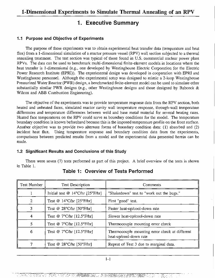
The purpose of these experiments was to obtain experimental heat transfer data (temperature and heat flux) from a 1-dimensional simulation of a reactor pressure vessel (RPV) wall section subjected to a thermal annealing treatment. The test section was typical of those found in U.S. commercial nuclear power plant RPVs. The data can be used to benchmark multi-dimensional finite-element models in locations where the heat transfer is 1-dimensional (e.g., one developed by Westinghouse Electric Corporation for the Electric Power Research Institute (EPRI)). The experimental design was developed in cooperation with EPRI and Westinghouse personnel. Although the experimental setup was designed to mimic a 2-loop Westinghouse Pressurized Water Reactor (PWR) design, a benchmarked finite-element model can be used to simulate other substantially similar PWR designs (e.g., other Westinghouse designs and those designed by Babcock & Wilcox and ABB Combustion Engineering).
The objective of the experiments was to provide temperature response data from the RPV section, both heated and unheated faces, simulated reactor cavity wall temperature response, through-wall temperature differences and temperature differences between weld and base metal material for several heating rates. Heated face temperatures on the RPV could serve as boundary conditions for the model. The temperature boundary condition is known beforehand because this is the imposed temperature profile on the front surface. Another objective was to provide two alternate forms of boundary condition data: (1) absorbed and (2) incident heat flux. Using temperature response and boundary condition data from the experiments, comparisons between predicted results from a model and the experimental data presented herein can be made.
1.2 Significant Results and Conclusions of this Study
There were seven (7) tests performed as part of this project. A brief overview of the tests is shown in Table 1.
Table 1: Overview of Tests Performed
Test Number Test Description Comments
1 Initial test @ 14°C/hr [25°F/hr] "Shakedown" test to "work out the bugs."
2 Test @ 14°C/hr [25°F/hr] First "good" test.
3 Test @ 28°C/hr [50°F/hr] Faster heat-up/cool-down rate
4 Test @ 7°C/hr [12.5°F/hr] Slower heat-up/cool-down rate
5 Test @ 7°C/hr [12.5°F/hr] Thermocouple mounting error check
6 Test @ 7°C/hr [12.5°F/hr] Thermocouple mounting error check at different heat-up/cool-down rate
7 Test @ 28°C/hr [50°F/hr] Repeat of Test 3 due to marginal data.
1-1

1-Dimensional Experiments to Simulate Thermal Annealing of an RPV
Figure 1 is a schematic of the test setup. The temperature profile shape imposed on the heated face of the RPV section is shown in Figure 2. Figures 6 and 16 (discussed later) provide more detailed information.
Concrete walI "Mirror" insulation
emperature
Heater banks
Air flow upward
RPV section
Figure 1. Schematic of the Test Setup.
454C [850F] "soak" temperature
7, 14, 28C/hr [12.5, 25, 50F/hr] temperature heat-up and coo I-down rates
i me Figure 2. Temperature Profile on the Heated Face of the RPV Section.
1-2
1-Dimensional Experiments to Simulate Thermal Annealing of an RPV 1.2.1 Significant Results
Temperature Control and RPV Section Temperature Uniformity
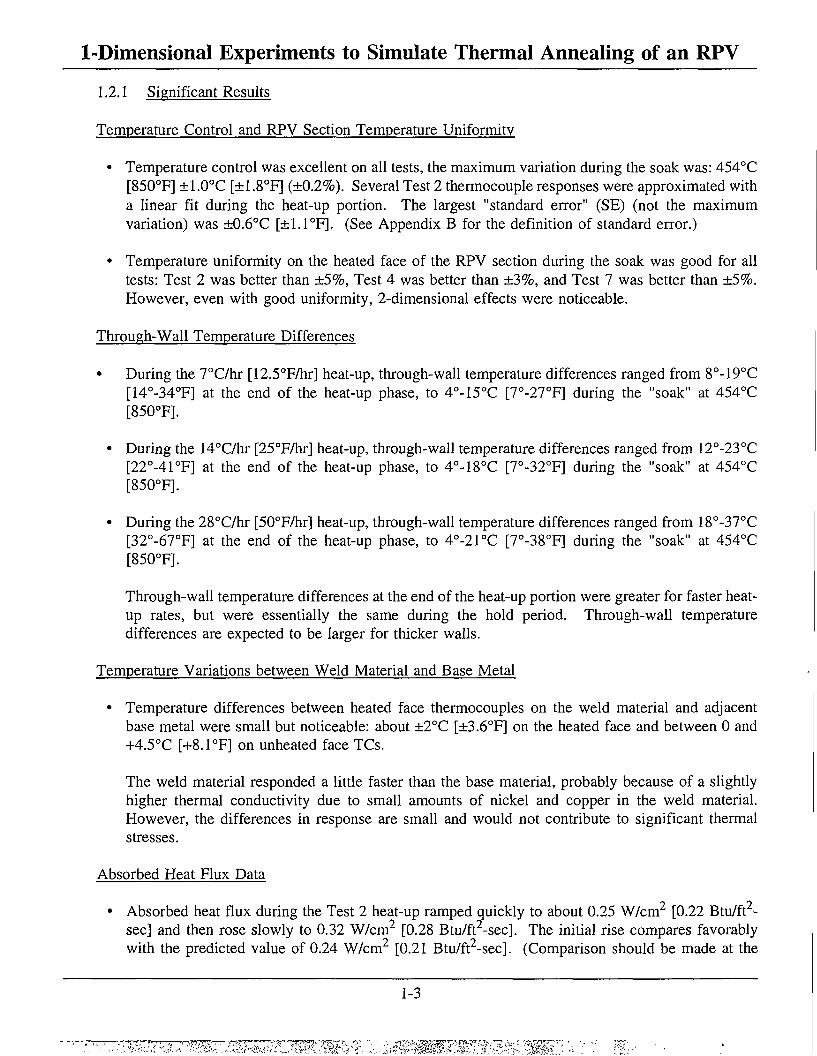
• Temperature control was excellent on all tests, the maximum variation during the soak was: 454°C [850°F] ±1.0°C [±1.8°F] (±0.2%). Several Test 2 thermocouple responses were approximated with a linear fit during the heat-up portion. The largest "standard error" (SE) (not the maximum variation) was ±0.6°C [±1.1°F]. (See Appendix B for the definition of standard error.)
• Temperature uniformity on the heated face of the RPV section during the soak was good for all tests: Test 2 was better than ±5%, Test 4 was better than ±3%, and Test 7 was better than ±5%. However, even with good uniformity, 2-dimensional effects were noticeable.
Through-Wall Temperature Differences
• During the 7°C/hr [12.5°F/hr] heat-up, through-wall temperature differences ranged from 8°-19°C [14°-34°F] at the end of the heat-up phase, to 4°-15°C [7°-27°F] during the "soak" at 454°C [850°F].
• During the 14°C/hr [25°F/hr] heat-up, through-wall temperature differences ranged from 12°-23°C [22°-41°F] at the end of the heat-up phase, to 4°-18°C [7°-32°F] during the "soak" at 454°C [850°F].
• During the 28°C/hr [50°F/hr] heat-up, through-wall temperature differences ranged from 18°-37°C [32°-67°F] at the end of the heat-up phase, to 4°-21°C [7°-38°F] during the "soak" at 454°C [850°F].
Through-wall temperature differences at the end of the heat-up portion were greater for faster heat-up rates, but were essentially the same during the hold period. Through-wall temperature differences are expected to be larger for thicker walls.
Temperature Variations between Weld Material and Base Metal
• Temperature differences between heated face thermocouples on the weld material and adjacent base metal were small but noticeable: about ±2°C [±3.6°F] on the heated face and between 0 and +4.5°C [+8.1°F] on unheated face TCs.
The weld material responded a little faster than the base material, probably because of a slightly higher thermal conductivity due to small amounts of nickel and copper in the weld material. However, the differences in response are small and would not contribute to significant thermal stresses.
Absorbed Heat Flux Data
• Absorbed heat flux during the Test 2 heat-up ramped quickly to about 0.25 W/cm [0.22 Btu/ft -sec] and then rose slowly to 0.32 W/cm2 [0.28 Btu/ft2-sec]. The initial rise compares favorably with the predicted value of 0.24 W/cm [0.21 Btu/ft2-sec]. (Comparison should be made at the
1-3
-•wa-'ju ^^::m^wcm^:m^w'-:-i^m^mm^m^:^mi^ • • ~
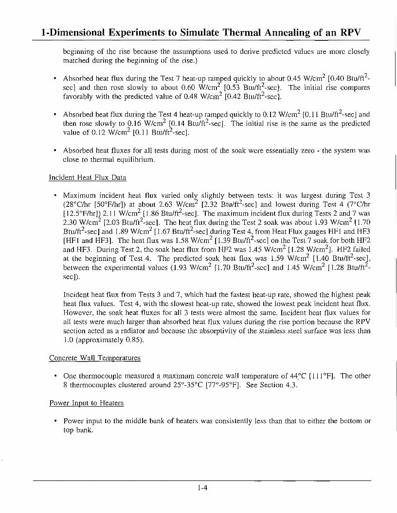
1-Dimensional Experiments to Simulate Thermal Annealing of an RPV beginning of the rise because the assumptions used to derive predicted values are more closely matched during the beginning of the rise.)
• Absorbed heat flux during the Test 7 heat-up ramped quickly to about 0.45 W/cm [0.40 Btu/ft -sec] and then rose slowly to about 0.60 W/cm [0.53 Btu/ft~-sec]. The initial rise compares favorably with the predicted value of 0.48 W/cm2 [0.42 Btu/ft2-sec].
• Absorbed heat flux during the Test 4 heat-up ramped quickly to 0.12 W/cm2 [0.11 Btu/ft -sec] and then rose slowly to 0.16 W/cm [0.14 Btu/ft~-sec]. The initial rise is the same as the predicted value of 0.12 W/cm2 [0.11 Btu/ft2-sec].
• Absorbed heat fluxes for all tests during most of the soak were essentially zero - the system was close to thermal equilibrium.
Incident Heat Flux Data
• Maximum incident heat flux varied only slightly between tests: it was largest during Test 3 (28°C/hr [50°F/hr]) at about 2.63 W/cm2 [2.32 Btu/ft2-sec] and lowest during Test 4 (7°C/hr [12.5°F/hr]) 2.11 W/cm2 [1.86 Btu/ft2-sec]. The maximum incident flux during Tests 2 and 7 was 2.30 W/cm2 [2.03 Btu/ft2-sec]. The heat flux during the Test 2 soak was about 1.93 W/cm2 [1.70 Btu/ft2-sec] and 1.89 W/cm2 [1.67 Btu/ft2-sec] during Test 4, from Heat Flux gauges HF1 and HF3 [HF1 and HF3]. The heat flux was 1.58 W/cm2 [1.39 Btu/ft2-sec] on the Test 7 soak for both HF2 and HF3. During Test 2, the soak heat flux from HF2 was 1.45 W/cm2 [1.28 W/cm2]. HF2 failed at the beginning of Test 4. The predicted soak heat flux was 1.59 W/cm2 [1.40 Btu/ft2-sec], between the experimental values (1.93 W/cm2 [1.70 Btu/ft2-sec] and 1.45 W/cm2 [1.28 Btu/ft2-sec]).
Incident heat flux from Tests 3 and 7, which had the fastest heat-up rate, showed the highest peak heat flux values. Test 4, with the slowest heat-up rate, showed the lowest peak incident heat flux. However, the soak heat fluxes for all 3 tests were almost the same. Incident heat flux values for all tests were much larger than absorbed heat flux values during the rise portion because the RPV section acted as a radiator and because the absorptivity of the stainless steel surface was less than 1.0 (approximately 0.85).
Concrete Wall Temperatures
• One thermocouple measured a maximum concrete wall temperature of 44°C [111°F]. The other 8 thermocouples clustered around 25°-35°C [77°-95°F]. See Section 4.3.
Power Input to Heaters
• Power input to the middle bank of heaters was consistently less than that to either the bottom or top bank.
1-4

1-Dimensional Experiments to Simulate Thermal Annealing of an RPV Thermocouple Mounting Method Errors
• Sheathed thermocouples (TCs) mounted on an RPV surface read higher than the RPV surface temperature, in this case up to 5°C [9°F], assuming the RPV temperature can be accurately measured using intrinsically mounted TCs. In an actual anneal, it will likely not be possible to attach TCs to the RPV surface, so the RPV temperature measurement has to be carefully made to prevent excessive errors.
Determination of Setpoint Temperature
• The RPV section was not all at the same temperature during the soak at the setpoint 454°C [850°F]. Typical variations around the setpoint were ±5%. In addition, thermocouple measurement errors may result in temperature measurements higher than the actual RPV temperature. These factors can be used in the determination of setpoint temperature.
1.2.2 Conclusions
1. Temperature uniformity on the heated face of the RPV section during the soak was good for all tests. Temperature control about the setpoint was excellent.
2. Through-wall temperature differences at the end of the heat-up portion were greater for higher heat-up rates, but were essentially the same during the hold period.
3. There were small but noticeable temperature differences between the response of the weld material and the base metal. However, the differences in response are very small and will likely not contribute to significant thermal stresses.
4. Incident heat fluxes for Tests 3 and 7, which had the fastest heat-up rate, were the highest. Test 4, with the slowest heat-up rate, shows the lowest incident heat flux. However, the soak time incident heat flux values for all tests were almost the same. Incident heat fluxes were consistently higher than absorbed fluxes, mainly because the RPV radiated heat away.
5. Absorbed heat fluxes generated by SODDIT agreed with predicted values at the beginning of the heat-up. However, the measured absorbed heat fluxes kept rising slowly after the initial sharp rise while the predicted values were constant (due to an adiabatic boundary condition assumption). Absorbed heat flux on all tests dropped to zero during the soak.
6. The maximum concrete wall temperature measured was 44°C [111°F] or less for all tests. If this is the case in an actual anneal, the concrete wall may not sustain any damage.
7. Power input to the middle bank of heaters was consistently less than that to either the bottom or top bank. This suggests that, during an actual anneal, the heaters facing the middle portion of the RPV being annealed would require less power than those heaters above and below. In addition, heaters facing areas of the RPV with large heat sinks will require additional power.
8. Sheathed thermocouples (TCs) mounted on an RPV surface read higher than the RPV surface temperature, in this case up to 5°C [9°F], assuming the RPV temperature can be accurately
1-5
1-Dimensional Experiments to Simulate Thermal Annealing of an RPV measured using intrinsically mounted TCs. In an actual anneal, it will likely not be possible to attach TCs to the RPV surface, so the RPV temperature measurement system/hardware has to be carefully designed and checked to prevent excessive errors.
9. Depending on the uniformity of the RPV temperature and error of the RPV temperature measurement, it may be desirable to increase the setpoint above 454°C [850°F] to ensure that a large fraction of the RPV will be annealed above some threshold temperature.
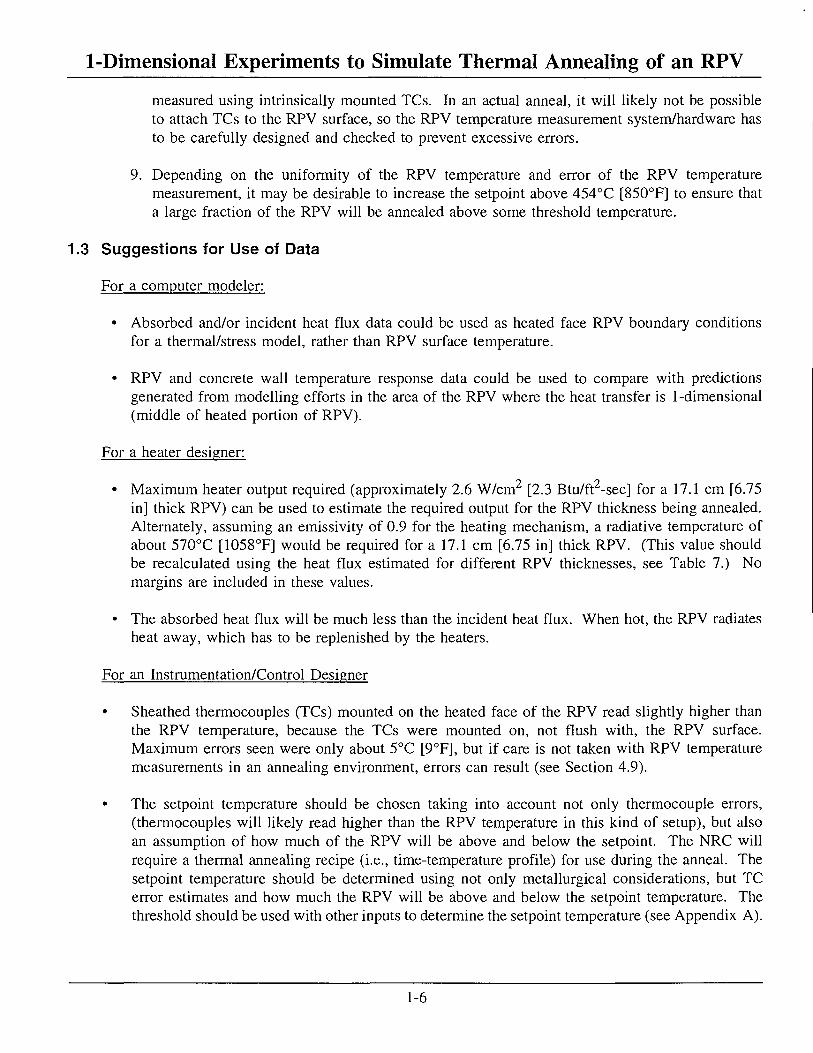
1.3 Suggestions for Use of Data
For a computer modeler:
• Absorbed and/or incident heat flux data could be used as heated face RPV boundary conditions for a thermal/stress model, rather than RPV surface temperature.
• RPV and concrete wall temperature response data could be used to compare with predictions generated from modelling efforts in the area of the RPV where the heat transfer is 1-dimensional (middle of heated portion of RPV).
For a heater designer:
• Maximum heater output required (approximately 2.6 W/cm [2.3 Btu/ft -sec] for a 17.1 cm [6.75 in] thick RPV) can be used to estimate the required output for the RPV thickness being annealed. Alternately, assuming an emissivity of 0.9 for the heating mechanism, a radiative temperature of about 570°C [1058°F] would be required for a 17.1 cm [6.75 in] thick RPV. (This value should be recalculated using the heat flux estimated for different RPV thicknesses, see Table 7.) No margins are included in these values.
• The absorbed heat flux will be much less than the incident heat flux. When hot, the RPV radiates heat away, which has to be replenished by the heaters.
For an Instrumentation/Control Designer
• Sheathed thermocouples (TCs) mounted on the heated face of the RPV read slightly higher than the RPV temperature, because the TCs were mounted on, not flush with, the RPV surface. Maximum errors seen were only about 5°C [9°F], but if care is not taken with RPV temperature measurements in an annealing environment, errors can result (see Section 4.9).
• The setpoint temperature should be chosen taking into account not only thermocouple errors, (thermocouples will likely read higher than the RPV temperature in this kind of setup), but also an assumption of how much of the RPV will be above and below the setpoint. The NRC will require a thermal annealing recipe (i.e., time-temperature profile) for use during the anneal. The setpoint temperature should be determined using not only metallurgical considerations, but TC error estimates and how much the RPV will be above and below the setpoint temperature. The threshold should be used with other inputs to determine the setpoint temperature (see Appendix A).
1-6
1-Dimensional Experiments to Simulate Thermal Annealing of an RPV
2. Introduction
2.1 Background
The continued viability of the nuclear power option (i.e., continued operation of existing plants for up to 60 years, or the next generation of plants) is very dependent on the continued safe and economic operation of existing plants without premature shutdown. The resolution of RPV neutron radiation embrittlement issues, in a cost-effective manner without excessive conservatism due to a lack of clear scientific information, is critical given the RPV's safety significance and high replacement cost.
Several options exist to manage the embrittlement of RPV materials. These options can be grouped into four categories [1]:
1. demonstrate embrittlement susceptibility to be less than predicted, 2. reduce the embrittlement rate, 3. remove the embrittlement, and 4. demonstrate plant-specific variables permit greater levels of acceptable embrittlement.
Category 1 includes, for example, an enhanced surveillance program to obtain more knowledge of the actual critical material irradiation exposure. This information could be used to reduce uncertainty in subsequent analyses to predict embrittlement trends. Category 2 involves flux reduction techniques including fuel management, shielding, and derating. Category 3 includes thermal annealing, RPV weld replacement, and RPV replacement. Category 4 includes techniques to demonstrate the benefit of particular plant conditions (i.e., analytical methods to demonstrate continued RPV integrity under specified loading conditions).
Thermal annealing, as described in Category 3, is a method of RPV embrittlement management that results in the removal of neutron radiation damage. In fact, it is the only mitigative measure that restores the mechanical properties of RPV materials. Thermal annealing, as applied to a commercial RPV, would not be required on the entire RPV. Commercial RPV annealing would concentrate on the beltline or core region where embrittlement is the greatest. RPV annealing temperatures are expected to range from approximately 343°-480°C [650°-900°F]. The effectiveness of a thermal annealing treatment in recovering material properties will depend upon the original RPV irradiation temperature, annealing temperature, annealing time at temperature ("hold" time), original material chemistry, and the degree of embrittlement prior to annealing [2], [3]. A number of thermal anneals have been performed in the Former Soviet Union, Belgium [4], [5], and by the U.S. only for military reactors [6].
The technical feasibility of annealing commercial U.S. vessels has been studied [3],[7]. Based on these preliminary studies, annealing of U.S. RPVs is technically viable. More recently, thermal annealing has also been shown to be economically desirable under certain embrittlement management scenarios [1]. However, only limited detailed material performance data and information characterizing the general response of the RPV and surrounding components to the annealing treatment have been established to support these preliminary studies. This suggests the need to perform additional confirmatory metallurgical and material behavior research, develop an appropriate annealing process, and ultimately demonstrate thermal annealing technology on a commercial U.S. RPV.
2-1
1-Dimensional Experiments to Simulate Thermal Annealing of an RPV The U.S. Department of Energy (DOE) Plant Lifetime Improvement (PLIM) Program, through DOE's
Light Water Reactor (LWR) Technology Center at Sandia National Laboratories, is pursuing the technical demonstration of annealing commercial U.S. RPVs through a cooperative effort with the nuclear industry. Activities are presently under way through the DOE PLIM Program to perform confirmatory metallurgical and general material behavior research in support of U.S. nuclear industry efforts to ultimately demonstrate thermal annealing technology on a commercial U.S. RPV.
One part of the overall PLIM annealing effort is to provide heat transfer boundary condition and thermal response data that can be used to benchmark numerical/analytical models used to characterize and predict RPV response (thermally induced stresses and strains) during an annealing treatment. For example, EPRI has contracted with Westinghouse Electric Corporation (W) to develop a "detailed finite element model" to describe the annealing process. DOE's LWR Technology Center at Sandia agreed to assist in the model development by performing a series of experiments. The experiments simulated a 1-dimensional annealing treatment on a section of an RPV (the RPV is curved, but the heat transfer is nearly 1-dimensional) using electric resistance heaters similar to those used in anneals performed in the Former Soviet Union. The data apply to the middle of the heated portion of the RPV being annealed. Data gathered would provide input to a modeler to help benchmark assumptions made regarding heat transfer boundary conditions. In addition, temperature response of the RPV section and response of the simulated reactor cavity wall could be used to verify results of the modeling effort.
2.2 Contents of Report
Following Section 2, Introduction, Section 3, Test Setup and Instrumentation, discusses the following items:
3.1 RPV Section 3.2 Heater Design 3.3 Overall Test Setup 3.4 Instrumentation/Measurements 3.5 Temperature Profiles Imposed on Heated Face of the RPV Section
Section 4, Results/Data Analysis/Discussion, contains a presentation and discussion of the data:
4.1 Data Analysis Overview 4.2 Data Presented 4.3 Test 2: 14°C/hr [25°F/hr] 4.4 Tests 3 and 7: 28°C/hr [50°F/hr] 4.5 Test 4: 7°C/hr [12.5°F/hr] 4.6 Air Flow Data 4.7 Power Input to Heaters 4.8 2-Dimensional Effects 4.9 Measurement Errors/Uncertainties 4.10 General Discussion
Section 5, Conclusions and Other Information, provides several useful conclusions for computer code modelers and annealing apparatus designers. Section 6 lists References. Appendix A, RPV Temperature Variation: Effect on Control Temperature, discusses the variation in temperature on the front surface, and
2-2

1-Dimensional Experiments to Simulate Thermal Annealing of an RPV how that variation may affect the effectiveness of the anneal, assuming a minimum threshold temperature is required for a successful anneal. Using Gaussian ("normal") distribution assumptions, the setpoint should be increased by a certain amount to effect a minimum temperature on a large portion (over 99%) of the RPV surface. Appendices B and C contain Acronyms and Abbreviations, and Nomenclature, respectively.
2-3
1-Dimensional Experiments to Simulate Thermal Annealing of an RPV
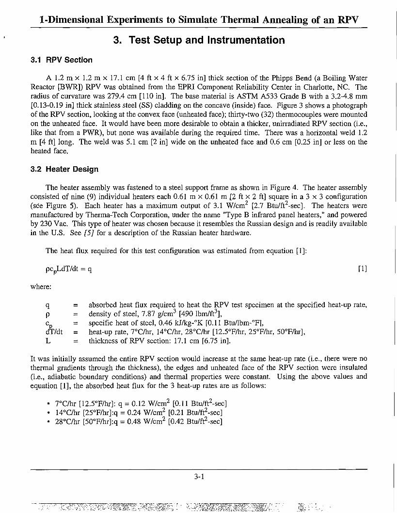
3. Test Setup and Instrumentation 3.1 RPV Section
A 1.2 m x 1.2 m x 17.1 cm [4 ft x 4 ft x 6.75 in] thick section of the Phipps Bend (a Boiling Water Reactor [BWR]) RPV was obtained from the EPRI Component Reliability Center in Charlotte, NC. The radius of curvature was 279.4 cm [110 in]. The base material is ASTM A533 Grade B with a 3.2-4.8 mm [0.13-0.19 in] thick stainless steel (SS) cladding on the concave (inside) face. Figure 3 shows a photograph of the RPV section, looking at the convex face (unheated face); thirty-two (32) thermocouples were mounted on the unheated face. It would have been more desirable to obtain a thicker, unirradiated RPV section (i.e., like that from a PWR), but none was available during the required time. There was a horizontal weld 1.2 m [4 ft] long. The weld was 5.1 cm [2 in] wide on the unheated face and 0.6 cm [0.25 in] or less on the heated face.
3.2 Heater Design
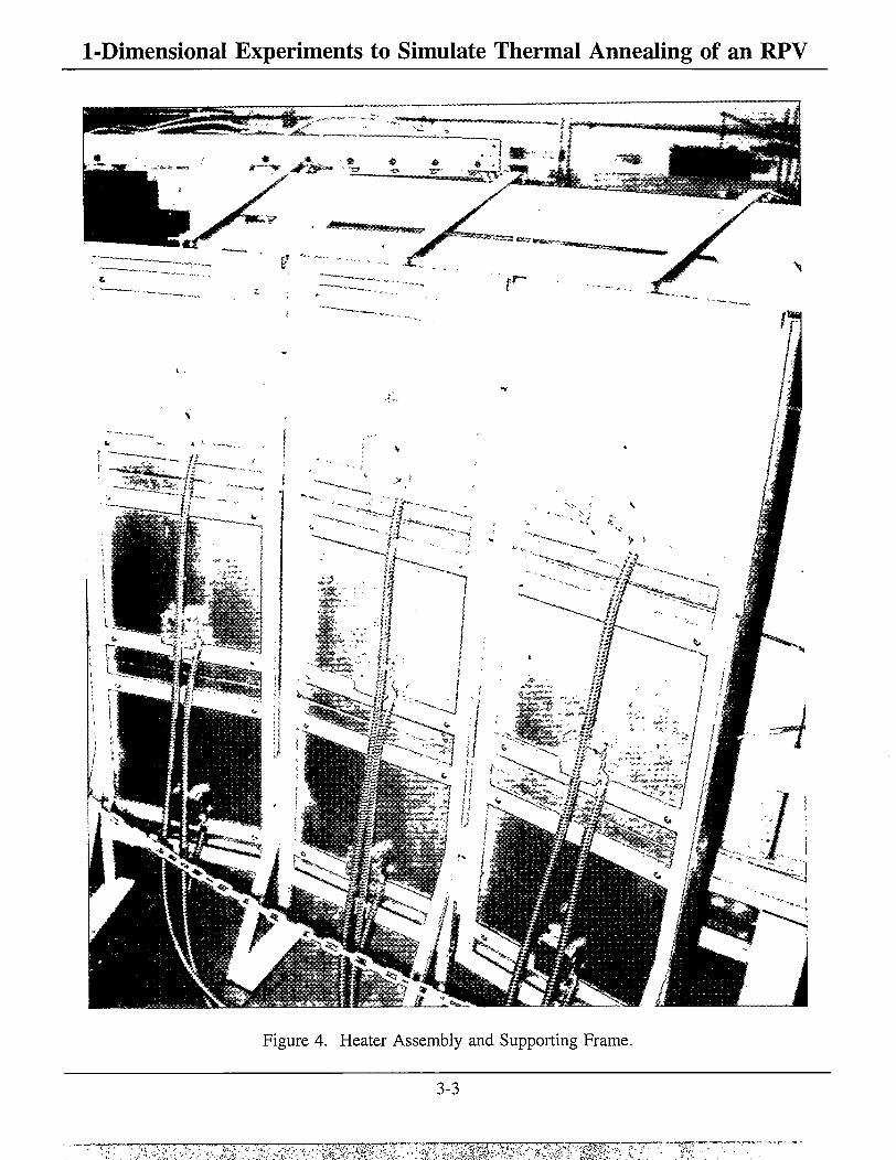
The heater assembly was fastened to a steel support frame as shown in Figure 4. The heater assembly consisted of nine (9) individual heaters each 0.61 m x 0.61 m [2 ft x 2 ft] square in a 3 x 3 configuration (see Figure 5). Each heater has a maximum output of 3.1 W/cm [2.7 Btu/ft -sec]. The heaters were manufactured by Therma-Tech Corporation, under the name "Type B infrared panel heaters," and powered by 230 Vac. This type of heater was chosen because it resembles the Russian design and is readily available in the U.S. See [5] for a description of the Russian heater hardware.
The heat flux required for this test configuration was estimated from equation [1]:
pcpLdT/dt = q [1]
where:
q = absorbed heat flux required to heat the RPV test specimen at the specified heat-up rate, p = density of steel, 7.87 g/cm3 [490 lbm/ft3], c = specific heat of steel, 0.46 kJ/kg-°K [0.11 Btu/lbm-°F], dT/dt = heat-up rate, 7°C/hr, 14°C/hr, 28°C/hr [12.5°F/hr, 25°F/hr, 50°F/hr], L = thickness of RPV section: 17.1 cm [6.75 in].
It was initially assumed the entire RPV section would increase at the same heat-up rate (i.e., there were no thermal gradients through the thickness), the edges and unheated face of the RPV section were insulated (i.e., adiabatic boundary conditions) and thermal properties were constant. Using the above values and equation [1], the absorbed heat flux for the 3 heat-up rates are as follows:
• 7°C/hr [12.5°F/hr]: q = 0.12 W/cm2 [0.11 Btu/ft2-sec] • 14°C/hr [25°F/hr]:q = 0.24 W/cm2 [0.21 Btu/ft2-sec] • 28°C/hr [50°F/hr]:q = 0.48 W/cm2 [0.42 Btu/ft2-sec]
3-1

Figure 3. Reactor Pressure Vessel (RPV) Section.
l-Dimensional Experiments to Simulate Thermal Annealing of an RPV
Figure 4. Heater Assembly and Supporting Frame.
3-3

1-Dimensional Experiments to Simulate Thermal Annealing of an RPV
Figure 5. Heater Modules in 3 x 3 Configuration.
3-4

1-Dimensional Experiments to Simulate Thermal Annealing of an RPV In the 1-dimensional experiments, there was non-negligible heat loss from the unheated face not
accounted for in equation [1]. Therefore, the absorbed heat flux required to effect the desired heat-up rate was not constant as indicated but rose slowly in a linear manner throughout the heat-up portion of the tests. Main sources of heat transfer from the unheated face were convection and radiation; the amount of extra energy required to account for heat losses was about 32% of the absorbed heat flux at the beginning of the heat-up. (See discussions of the absorbed heat flux data in Sections 4.3-4.5 and Table 7.)
At the time of the original design, the maximum expected heat-up was to be 14°C/hr [25°F/hr], therefore the design flux was 0.24 W/cm [0.21 Btu/ft -sec]. To allow for losses because the RPV was not insulated on the back side and to account for the fact that the absorptivity of the stainless steel surface of the RPV was less than 1.0 (typical value of absorptivity for weathered stainless steel (SS): a = 0.85), the heaters were designed with an order of magnitude reserve capacity (flux of 2.4 W/cm2 [2.1 Btu/ft2-sec]). The closest heater range available from the manufacturer was 3.1 W/cm [2.7 Btu/ft -sec], as indicated above. With this heater design, a 28°C/hr [50°F/hr] heat-up rate was also attainable.
The heater assembly was 1.83 m [6 ft] square whereas the test specimen was 1.22 m [4 ft] square. The 0.30 m [1 ft] overlap gave good uniformity of heating on the RPV section and made the tests more nearly 1-dimensional (although not totally 1-dimensional, as will be seen in Section 4.8). The heaters were placed nominally 25.4 cm [10 in] away from the RPV section, the same distances used in the Russian anneal described in [5]. The heaters were controlled by 3 power channels, therefore, there were 3 heaters per channel. Control was achieved by monitoring a single thermocouple per channel mounted in the center of each control zone and using that output to adjust the power to each set of 3 heater modules. Convective effects made the heat rise, so 3 heaters were connected in a row (rather than a column) to a single channel. The power channels were programmable, therefore, a desired temperature profile was set into the controller memory, and control was automatic. This was a desired feature because of the length of the tests, which ran overnight without personnel in attendance.
3.3 Overall Test Setup
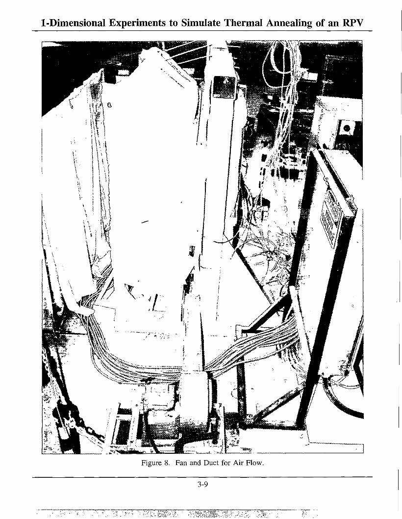
Figure 6 shows a side view of the entire test setup (not to scale). The test specimen and "mirror" insulation were mounted on a common steel supporting frame shown in Figure 7. The concrete wall was mounted in a separate frame also shown in Figure 7. Note that the mirror insulation was contoured to the shape of the RPV section, but the concrete wall was flat. Figure 8 shows the fan and duct placement in relation to the overall setup. The original duct used was a long, thin shape with a rectangular cross section. Due to poor air flow uniformity, the rectangular duct was changed to a circular design that resulted in much better air flow uniformity (see data in Section 4.6).
All edges of the RPV section were insulated with a ceramic-fiber type of high temperature insulation with low thermal conductivity. The insulation comes in both loose "batt" and rigid forms. The top, bottom, and sides of the space between the heater assembly and the RPV section were enclosed with batt insulation to simulate as close as possible the anticipated situation in an actual anneal. The underside of the RPV section was insulated with rigid insulation, as shown in Figure 7.
The unheated face of the RPV section was exposed to air but the edges were enclosed. There was an air gap 1.3-1.9 cm [0.5-0.75 in] wide between the RPV and the mirror insulation. In a typical plant layout (a 2-loop Westinghouse designed PWR), 7.6 cm [3 in] of a "sandwich" type of mirror insulation made of SS sheets with an aluminum foil filler is used. This type of insulation was prohibitively expensive. The
3-5
1-Dimensional Experiments to Simulate Thermal Annealing of an RPV thermal conductivity of this type of insulation is about twice that of the ceramic-fiber insulation described in the preceding paragraph . Therefore, about 3.8 cm [1.5 in] of the ceramic-fiber batt insulation was substituted for the more expensive kind (the ceramic-fiber batt is much less expensive). The batt was "sandwiched" between two polished aluminum sheets to simulate the "mirror" insulation (which is made of SS sheets) in an actual plant. The sheets were polished to produce a highly reflective surface. The insulation sandwich was placed near the back side of the RPV section.
The concrete wall was placed behind the mirror insulation to simulate a reactor cavity wall. This flat wall was solid concrete, 2.1 m x 2.1 m x 25.4 cm thick [7 ft x 7 ft x 10 in]. There was an air gap between the back side of the mirror insulation and the concrete wall. Because the insulation was contoured but the concrete wall was flat, the gap ranged from a minimum of 5.1 cm [2 in] in the middle to a maximum of 10.2 cm [4 in] at each side.
Air flowed upward in the space between the back of the RPV section and the concrete wall. Specifications from a Westinghouse 2-loop PWR called for maximum air flow of about 708 m /min [26,000 cubic feet per minute (CFM)] to a minimum of 131.7 m3/min [4650 CFM] at 36°C [100°F]. Assuming a 5.1 cm [2 in] gap surrounding a 4.1 m [160 in] diameter RPV (Westinghouse RPV diameters vary from 3.4-4.4 m [132-173 in]), the velocity through the gap would be about 1135 m/min [3725 ft/min at 26,000 CFM] and 203 m/min [666 ft/min at 4650 CFM], respectively. The measured flow velocity was near the lower value (203 m/min [666 ft/min], but within the specified range. See Section 4.7 for a detailed discussion of air flow data. Air flow on the low side would result in higher concrete temperatures, an upper bound.
Figure 9 shows a sketch of the top view of the setup. The curvature of the heater assembly matched the RPV section curvature as closely as possible.
The experiments were performed in the Radiant Heat Facility (RHF), at Sandia National Laboratories in Albuquerque, NM. Personnel from the Thermal Test Team of the Energetic & Environmental Test Department 2761 set up the hardware, performed the experiments, gathered the data, and generated the results.
Private communication between Rick Rishel, Westinghouse Electric Corporation, and Jim Nakos, Sandia National Laboratories, Spring 1993.
3-6

5.1 cm [2 in] min, 10.2 cm [4 in] max gap between concrete wall and insulation
Concrete walI to simulate RPV cavity 2.1 x 2.1 m x 25.4 cm thick — [7 x 7 ft x 10 in] 3.8 cm [1.5 in] thick mirror insulation
Instrumentation on heated face, unheated face, and concrete wa
Air cool ing duct
Air flow upwards between concrete walI and RPV walI. Velocity about 204 m/min [670 ft/min].
Insulated enclosure 1.9 cm [0.75 in] air gap
Heater elements in a 5 x 3 array configuration 25 cm [10 in] from RPV section
1.2 x 1.2 m x 17.1 cm [4 x 4 ft x 6.75 in] thick RPV section (A533B)
Figure 6. Side View Sketch of Test Setup.

1-Dimensional Experiments to Simulate Thermal Annealing of an RPV
Figure 7. "Mirror" Insulation, Concrete Wall, and Supporting Frame.
3-8
1-Dimensional Experiments to Simulate Thermal Annealing of an RPV
Figure 8. Fan and Duct for Air Flow.
3-9

Insulation enclosure
Typical "Infrared panel heater' 0.6 x 0.6 m [2 x 2 ft]"; 3.1 W/cm2 [2.7 Btu/ft2-sec]
0.6 m 279 cm [110 in] [ 2 f t ]
radius
9 heaters total in $x$ arrangement
"Mirror" insulation
1.2 x 1.2 m x 17.1 cm [4 x 4 f t x 6.75 in] th A533B RPV section, with 3.2-4.8 mm [1/8-3/16 in] SS cladding
5.1 cm [2 in] gap
2.1 x 2.1 m x 25.4 cm [7 x 7 ft x 10 in] concrete walI
10.2 cm [4 in]
Figure 9. Top View Sketch of Test Setup.

1-Dimensional Experiments to Simulate Thermal Annealing of an RPV 3.4 Instrumentation/Measurements
Figures 3 and 10 show photographs of the unheated (convex) and heated (concave) faces of the RPV section, with TCs installed. Figures 11-13 show instrumentation layouts on the heated face of the RPV section (Figure 11), the unheated face (Figure 12) and the concrete wall (Figure 13). Except for 3 heat flux gages (pyrheliometers), instrumentation were all type K (chromel-alumel) thermocouples (TCs). Type K TCs were chosen because the data acquisition system (DAS) at the RHF has a type K reference junction. Metal sheathed TCs were chosen over glass sheathed TCs for two reasons: the metal sheathed TCs are much more rugged and the glass sheathed is effective to only about 480°C [900°F], close to the 454°C [850°F] setpoint used. Because multiple tests were planned, the TCs might be handled a number of times. Also, because the setpoint temperature was close to the maximum operating temperature of the glass sheath, and we were not sure whether the 480°C [900°F] maximum would be exceeded, metal sheathed TCs were chosen. Table 2 briefly describes the advantages/disadvantages of the two types of TCs.
Table 2: Advantages/Disadvantages of Thermocouple Types Thermocouple
Sheath Material Advantages Disadvantages
Metal (stainless steel, inconel)
Rugged, stable Measuring junction not in direct contact with surface to be measured, unless sheath stripped away
Glass (fiberglass) Light, able to weld directly to surface being measured
Prone to failure, wires kink, glass insulation breaks down and faulty measurements result, even though the measurement looks reasonable
It is desirable to use the smallest TC possible, because the TC disturbs the surface being measured and because smaller TCs possess better transient response. Metal sheathed TCs are manufactured in many sizes: 0.51 mm [0.020 in], 1.02 mm [0.040 in], 1.6 mm [0.063 in], and larger diameters. Experience has shown that 1.6 mm [0.063 in] diameter stainless steel TCs offer a good combination of transient response, ruggedness, and cost. Therefore, they are stocked for use at the RHF.
Another consideration regarding TC selection is the method used to mount the measuring junction to the measuring surface. Experience has showed that the mounting method with the least error consists of directly welding each wire (chromel and alumel) to the surface being measured. This provides good thermal contact and is called an "intrinsic" TC. Data in Section 4.9 show that temperature differences between intrinsically mounted thermocouples and sheathed thermocouples are less than 4°C [7°F].
The only way to create an intrinsic TC with a metal sheathed TC is to strip away the sheath close to the measuring junction at the tip. This is called an "exposed" junction TC (which is equivalent to an intrinsically mounted TC). However, after the metal sheath is stripped away, the magnesium oxide (MgO) insulation separating the chromel and alumel wires from the sheath is exposed to the environment (dust, humidity). The electrical insulating properties of the MgO insulation when contaminated with moisture or dust are degraded. Electrical shorts can occur, therefore, although an exposed (intrinsic) junction is the best mounting method, it is not always reliable and can give reasonable but erroneous readings. For the above reasons, fully sheathed TCs were used.
3-11

1-Dimensional Experiments to Simulate Thermal Annealing of an RPV
r"*T?
a t-.
PL, -c o ex ex 3
00 c o •o o c 3 o
G O
4—» o <u 00 > OH OH
l-H
3 E
3-12
30.5 cm [12 in], typical
i
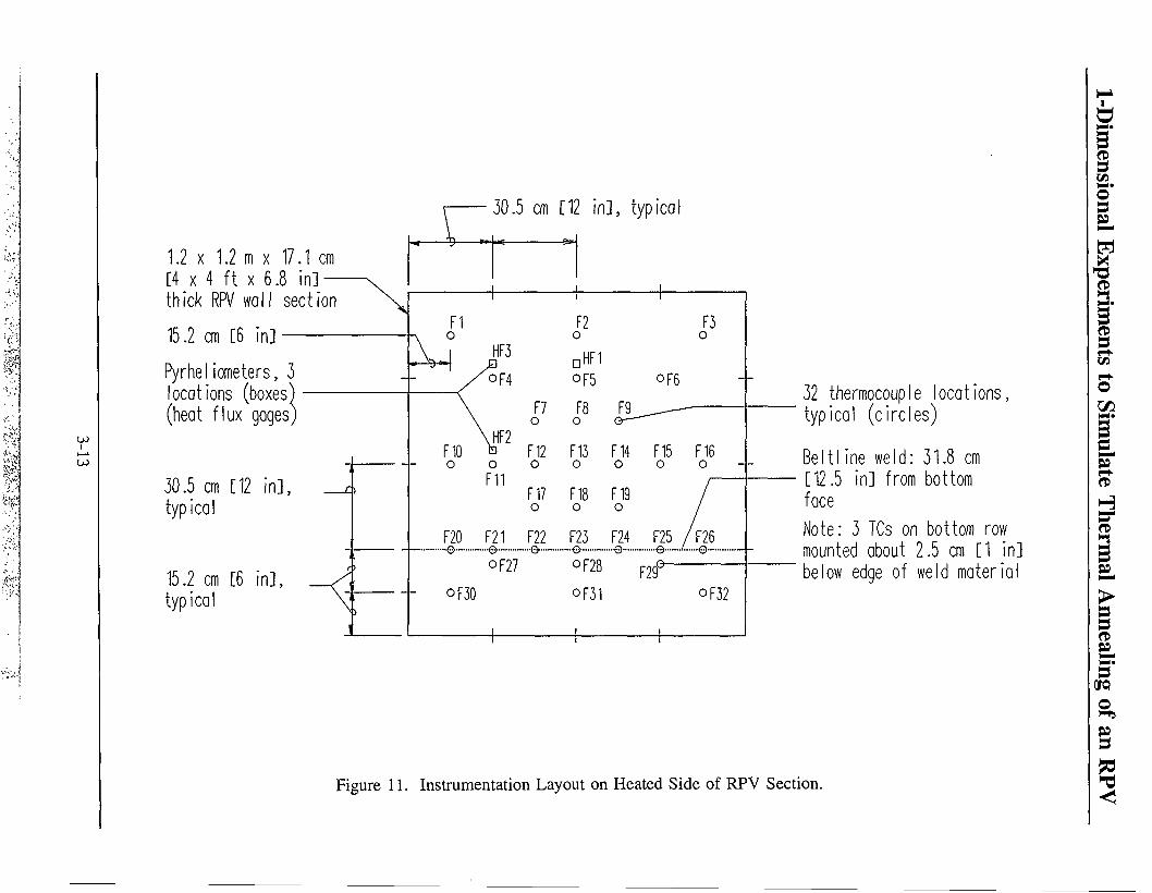
1.2 x 1.2 m x 17.1 cm [4 x 4 ft x 6.8 i n ] -thick RPV wall section 15.2 cm [6 in] Pyrheliometers, 3 locations (boxes) (heat flux gages)
30.5 cm [12 in], typical
15.2 cm [6 in], typical
32 thermocouple locations, typical (circles)
Beltl ine weld: 31.8 cm [12.5 in] from bottom face Note: 3 TCs on bottom row mounted about 2.5 cm [1 in] below edge of weld material
Figure 11. Instrumentation Layout on Heated Side of RPV Section.

I
1.2 x 1.2 m x 17.1 cm [4 x 4 ft x 6.8 in] — thick RPV walI section 15.2 cm [6 in]
30.5 cm [12 in], typical
15.2 cm [6 in] typical
B3
116 o
30.5 cm [12 in], typical
B2
oB6
o B15
B25 ••••©
O R :
B9 o
B14 o
B24 ••••e-
o
oB5
B13 o
o
B23 ••••©
°B28
oB31
111 B12 o
B17 o
B22 B2' ™0 ©•••
B2f
no
32 thermocouple locations, typical (circles)
Belt I ine weld: 31.8 cm [12.5 in] from bottom face Note: 3 TCs on bottom row mounted about 2.5 cm [1 in] below edge of weld material
Figure 12. Instrumentation Layout on Unheated Side of RPV Section.
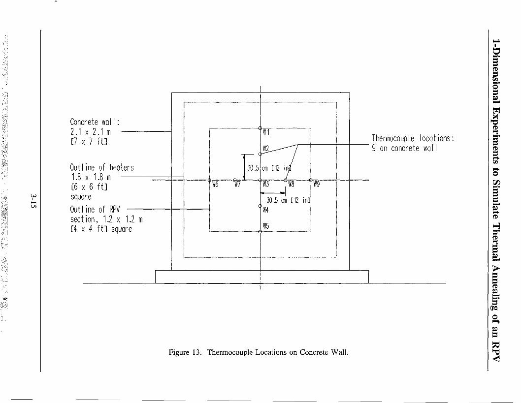
Concrete wall 2.1 x 2.1m [7 x 7 ft]
Out I ine of heaters 1.8 x 1.8 m [6 x 6 ft] square Outline of RPV section, 1.2 x 1.2 m [ 4 x 4 ft] square
Thermocouple locations: 9 on concrete walI
Figure 13. Thermocouple Locations on Concrete Wall.
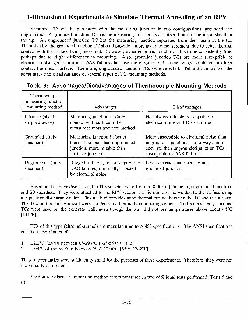
1-Dimensional Experiments to Simulate Thermal Annealing of an RPV Sheathed TCs can be purchased with the measuring junction in two configurations: grounded and
ungrounded. A grounded junction TC has the measuring junction as an integral part of the metal sheath at the tip. An ungrounded junction TC has the measuring junction separated from the sheath at the tip. Theoretically, the grounded junction TC should provide a more accurate measurement, due to better thermal contact with the surface being measured. However, experience has not shown this to be consistently true, perhaps due to slight differences in mounting. Also, grounded junction TCs are more susceptible to electrical noise generation and DAS failures because the chromel and alumel wires would be in direct contact the metal surface. Therefore, ungrounded junction TCs were selected. Table 3 summarizes the advantages and disadvantages of several types of TC mounting methods.
Table 3: Advantages/Disadvantages of Thermocouple Mounting Methods Thermocouple
measuring junction mounting method Advantages Disadvantages
Intrinsic (sheath stripped away)
Measuring junction in direct contact with surface to be measured; most accurate method
Not always reliable, susceptible to electrical noise and DAS failures
Grounded (fully sheathed)
Measuring junction in better thermal contact than ungrounded junction, more reliable than intrinsic junction
More susceptible to electrical noise than ungrounded junctions, not always more accurate than ungrounded junction TCs, susceptible to DAS failures
Ungrounded (fully sheathed)
Rugged, reliable, not susceptible to DAS failures, minimally affected by electrical noise.
Less accurate than intrinsic and grounded junction
Based on the above discussion, the TCs selected were 1.6 mm [0.063 in] diameter, ungrounded junction, and SS sheathed. They were attached to the RPV section via nichrome strips welded to the surface using a capacitive discharge welder. This method provides good thermal contact between the TC and the surface. The TCs on the concrete wall were bonded via a thermally conducting cement. To be consistent, sheathed TCs were used on the concrete wall, even though the wall did not see temperatures above about 44°C [111°F].
TCs of this type (chromel-alumel) are manufactured to ANSI specifications. The ANSI specifications call for uncertainties of:
1. ±2.2°C [±4°F] between 0°-293°C [32°-559°F], and 2. ±3/4% of the reading between 293°-1256°C [559°-2282°F].
These uncertainties were sufficiently small for the purposes of these experiments. Therefore, they were not individually calibrated.
Section 4.9 discusses mounting method errors measured in two additional tests performed (Tests 5 and 6).
3-16
1-Dimensional Experiments to Simulate Thermal Annealing of an RPV As Figure 11 shows, 32 TCs were mounted on the heated face. The bulk of the TCs were concentrated
in the center where the heat transfer was closest to 1-dimensional (to minimize "edge" effects). The EPRI Component Reliability Center did not want the RPV section damaged; therefore, practical considerations limited heat flux gage types that could be used. Disk shaped "pyrheliometers" were used (3.8 cm diameter x 1.9 cm thick [1.5 in diameter x 0.75 in thick]) to measure incident heat flux. Directly next to each pyrheliometer was a TC. The TC was used to estimate the total (convective + radiative) absorbed flux, whereas the pyrheliometer was used to measure the total (radiative + convective) incident flux to the heated face. Either incident or absorbed heat flux can be used by a modeler as a boundary condition input to determine the response of the RPV section and the thermal stresses generated. The incident heat flux from the pyrheliometers can also be used by a heater designer to estimate the size of the heaters required. As will be seen in the results section, the incident and absorbed fluxes were very different.
Referring to Figure 11, the control thermocouple for the top bank of heaters was F2, for the center bank of heaters, F13, and for the bottom bank, F31. Three (3) Research Incorporated "MicRIstar" Model 828E digital controllers were used to control the three heater banks (see Figure 14) via Research Incorporated Model 646 "Phaser" power controllers.
Figure 12 shows the TC layout on the unheated face. Except for the pyrheliometers, the layout is exactly the same as that on the heated face. Thirty-two (32) TCs were mounted on the unheated face. This allowed estimation of temperature gradients through the RPV section thickness as well as estimates of absorbed heat flux from unheated face measurements.
Note that predicted values of absorbed heat flux on the heated face can be obtained from TCs mounted on both the heated and unheated faces by use of the inverse heat conduction code SODDIT. This redundancy was intentional.
Figure 13 shows the TC layout on the concrete wall behind the RPV section. Nine (9) TCs were mounted on the concrete surface. This number was sufficient to obtain a temperature map and estimate the maximum temperature.
Three (3) water cooled pyrheliometers (heat flux gages) were used to measure heat flux incident on the heated RPV section surface. Figure 15 shows a photograph of the 3 pyrheliometers mounted in place. This type of gage is typically used in solar energy applications to measure radiative heat flux, but were configured to measure total heat flux (radiative + convective) in these experiments. The pyrheliometers would provide the incident heat flux measurements necessary to provide data on one of the alternate boundary conditions stated in the Introduction.
The pyrheliometers were selected on the basis of size/configuration and heat flux range. There are few transducers manufactured that can measure incident heat flux in the range of these experiments (1 W/cm [0.88 But/ft -sec]) This is in the range of solar energy heat flux at the earth's surface. In addition, there are no other known heat flux gage transducers than have the size and configuration required in these experiments. Because we could not penetrate the RPV section surface, the gages had to be surface mounted. Because there was only 25.4 cm [10 in] between the heaters and the RPV section surface, the gages had to be thin with the transducer measuring surface close to the RPV heated face.
3-17
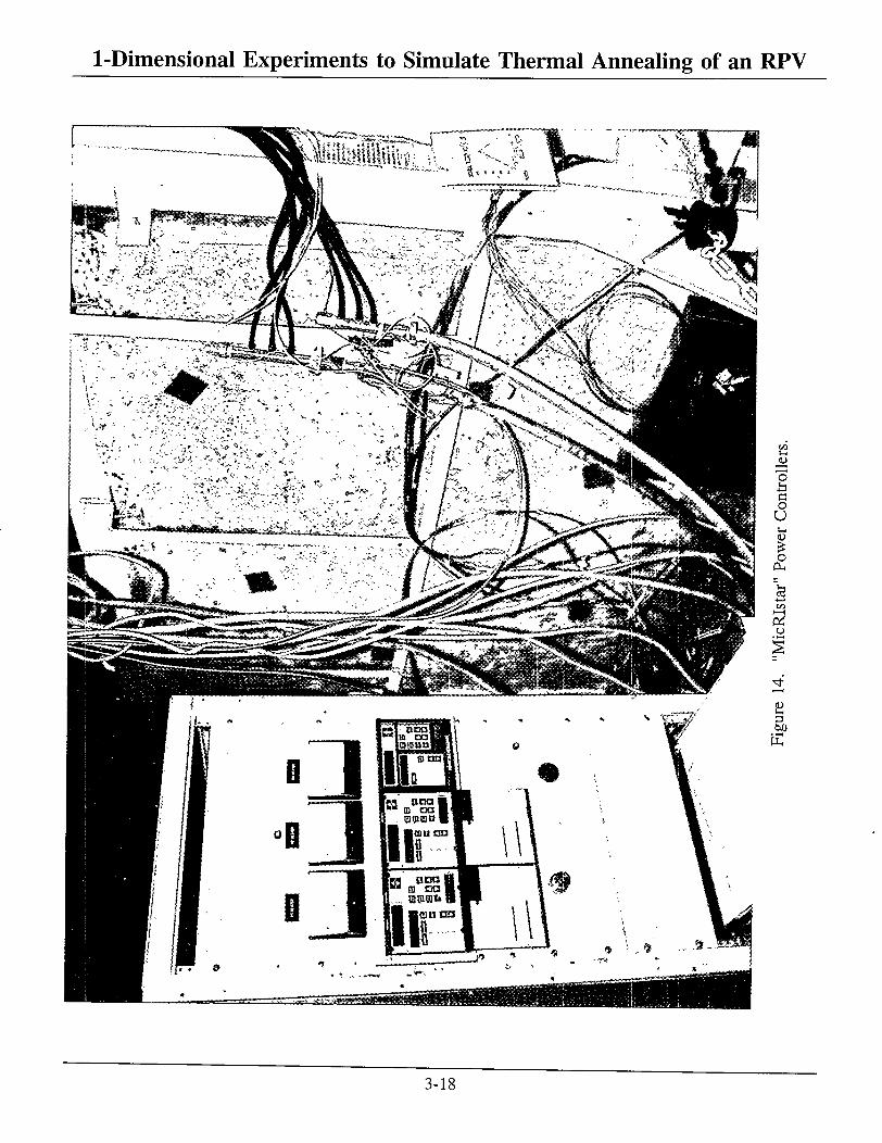
1-Dimensional Experiments to Simulate Thermal Annealing of an RPV
in
"o •-, • 4 — » c o U
O
ISO
3-18

1-Dimensional Experiments to Simulate Thermal Annealing of an RPV
Figure 15. Pyrheliometers Mounted on Heated Face.
3-19
1-Dimensional Experiments to Simulate Thermal Annealing of an RPV The gages chosen were manufactured by HY-CAL Engineering and are called "HY-THERM"
pyrheliometers, Model P-8400. The stated uncertainty of these gages in solar energy applications is ±3% in their normal application. However, because the gages were not used to measure incident heat flux from a solar energy source, the total uncertainty was a little higher: +3%, -6% 2 . This slight increase in uncertainty is due to a decrease in the absorptivity of the coating on the surface of the pyrheliometer for longer wavelengths (solar energy is at shorter wavelengths than the energy from the heaters). They were not placed directly in the center because the insulated water cooling lines were so bulky that too much of the RPV surface would have been covered. Each transducer comes with a calibration sheet of mV output versus incident heat flux. This calibration sheet has to be manually converted to a linear equation for use in data reduction. The stated linearity of the calibration is ±3%.
The power to each of the heater elements was recorded so that an additional estimation of heat flux output could be made (if needed) and to determine the uniformity of the power input to the heater banks. The power was estimated using an special circuit designed and fabricated at SNL's RHF for the power controllers used. The power measured is a true, instantaneous power value (volts*amps*cos(9)). The heaters are purely resistive, but there is a phase angle between the current and voltage due to the controllers used (Research Incorporated "Phaser" controllers).
Air flow velocity was measured with a handheld device called a "velometer." Details of these measurements are discussed in Section 4.6.
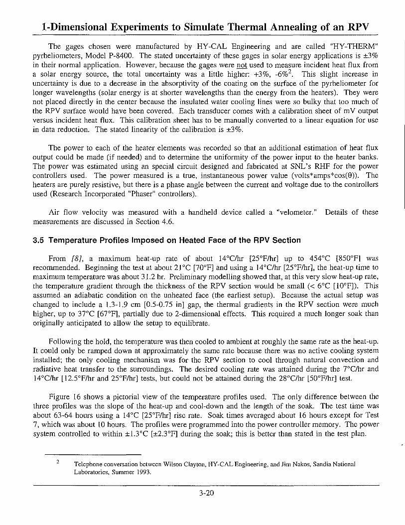
3.5 Temperature Profiles Imposed on Heated Face of the RPV Section
From [8], a maximum heat-up rate of about 14°C/hr [25°F/hr] up to 454°C [850°F] was recommended. Beginning the test at about 21°C [70°F] and using a 14°C/hr [25°F/hr], the heat-up time to maximum temperature was about 31.2 hr. Preliminary modelling showed that, at this very slow heat-up rate, the temperature gradient through the thickness of the RPV section would be small (< 6°C [10°F]). This assumed an adiabatic condition on the unheated face (the earliest setup). Because the actual setup was changed to include a 1.3-1.9 cm [0.5-0.75 in] gap, the thermal gradients in the RPV section were much higher, up to 37°C [67°F], partially due to 2-dimensional effects. This required a much longer soak than originally anticipated to allow the setup to equilibrate.
Following the hold, the temperature was then cooled to ambient at roughly the same rate as the heat-up. It could only be ramped down at approximately the same rate because there was no active cooling system installed; the only cooling mechanism was for the RPV section to cool through natural convection and radiative heat transfer to the surroundings. The desired cooling rate was attained during the 7°C/hr and 14°C/hr [12.5°F/hr and 25°F/hr] tests, but could not be attained during the 28°C/hr [50°F/hr] test.
Figure 16 shows a pictorial view of the temperature profiles used. The only difference between the three profiles was the slope of the heat-up and cool-down and the length of the soak. The test time was about 63-64 hours using a 14°C [25°F/hr] rise rate. Soak times averaged about 16 hours except for Test 7, which was about 10 hours. The profiles were programmed into the power controller memory. The power system controlled to within ±1.3°C [±2.3°F] during the soak; this is better than stated in the test plan.
Telephone conversation between Wilson Clayton, HY-CAL Engineering, and Jim Nakos, Sandia National Laboratories, Summer 1993.
3-20

1-Dimensional Experiments to Simulate Thermal Annealing of an RPV
454C [850F]
Temperature, degrees C [F]
21C [70F]
Hold time varied, 16 hours for Tests 2, 3 and 4; 10 hrs for Test 7
7, 14 or 28C/hr [12.5, 25 or 50F/hr] temperature rise rate and coo I down"rate —
30 Time.
60 90
hours (for 28C/hr rise rate)
Figure 16. Temperature Profile Imposed on Heated Face of RPV Section.
A total of 7 tests were completed. All tests heated up to a soak temperature of 454°C [850°F]. The first test used a nominal heat-up rate of 14°C/hr [25°F/hr]. A few minor problems were discovered during Test 1, a "shakedown" test. The air flow was not sufficiently uniform, the soak was not long enough and the upper left corner of the RPV section, looking from the heated face, was slightly cooler than the remainder of the RPV. A circular (rather than rectangular) duct was fabricated and tested. The air flow was much more uniform. The soak at maximum temperature was increased to allow both the RPV section and the concrete wall to reach thermal equilibrium. In order to correct the slight cool spot on the RPV section, edges of the 1.3-1.9 cm [0.5-0.75 in] air gap were covered with insulation (this gap was not enclosed on the check test). These improvements solved the non-uniform air flow and the soak problems, but the cool spot in the upper left corner of the RPV section was still present. However, as will be seen, the temperature uniformity was better than ±5% on all tests; this was sufficiently uniform for the purposes of these experiments. After all of the testing was completed, a close examination of the setup revealed that the heaters facing the upper left corner of the RPV section were slightly farther (3.2 cm [1.3 in]) away from than those facing other parts of the setup; this may have caused the cool spot.
3-21
1-Dimensional Experiments to Simulate Thermal Annealing of an RPV After the shakedown test, improvements were made to the setup, the next three (3) tests were performed
in the following order:
Test 2: 14°C/hr [25°F/hr] Test 3: 28°C/hr [50°F/hr] Test 4: 7°C/hr [12.5°F/hr]
The RPV was held at 454°C [850°F] until the concrete wall temperatures equilibrated at their maxima, then cooldown began. The 28°C/hr [50°F/hr] rise rate was proposed so that we could examine a larger through-wall temperature difference. The 7°C/hr [12.5°F/hr] test was performed to examine a smaller through-wall temperature difference. These tests are described in Sections 4.3-4.5.
Tests 5 and 6 were tests designed to check for thermocouple mounting errors. Five intrinsic TCs, identical to sheathed TCs except for the mounting method, were placed adjacent to sheathed TCs F10, Fl 1, F12, F13, and F14. The Test 5 heat-up rate was 7°C/hr [12.5°F/hr], and for Test 6 was 14°C/hr [25°F/hr]. Results of these tests are described in Section 4.9.
Test 7 was a repeat of Test 3, at 28°C/hr [50°F/hr]. During data analysis of Test 3, it was determined that one of the controllers malfunctioned, causing non-uniform soak temperatures. Therefore, the test was repeated. Data from Tests 3 and 7 are discussed in Section 4.5.
3-22

1-Dimensional Experiments to Simulate Thermal Annealing of an RPV 4. Results/Data Analysis/Discussion
4.1 Data Analysis Overview
Table 4 gives an overview of the a) measurements made, b) data reduction plan, and c) final output. Details are given below.
Table 4: Data Analysis/Data Reduction Plan
Transducer/ Measurement Data Reduction Final Output
TC/heated face temperature
Use TC data from heated face as input to SODDIT1 to estimate heat flux absorbed into heated face of RPV test specimen.
Plots of temperature versus time at 32 locations on heated face. Plots of absorbed heat flux versus time for 32 locations on heated face.
TC/unheated face temperature
Use TC data from unheated face as input to SODDIT to estimate heat flux absorbed into heated face of RPV test specimen.
Plots of unheated face temperature versus time for 32 locations. Plots of absorbed heat flux on heated face versus time for 32 locations, used as backup.
TC/heated and unheated face temperatures
Through-wall temperature differences obtained from "opposed" (heated/unheated face) TCs.
Plots of temperature differences through the wall thickness as measured from the heated and unheated face TCs.
TC/concrete wall temperature
Direct measure of concrete wall temperature.
Plots of temperature versus time for 9 locations on concrete wall.
Pyrheliometer2/ heated face
Direct measure of incident heat flux on heated face.
Plots of incident heat flux on heated face for 3 locations.
Velometer/air flow velocity
Average values from several tests at 5 measurement locations
Average air flow velocity
Power circuit/ kW to heaters
Direct measure of heater power. Heater power versus time.
SODDIT = Sandia One Dimensional Direct and Inverse Thermal computer code.
Pyrheliometer = a type of heat flux gage that can measure incident values of heat flux typical of these experiments. These are typically used in solar energy applications to measure the radiative component of heat flux but were configured to measure the sum of radiative and convective heat transfer.
4-1

1-Dimensional Experiments to Simulate Thermal Annealing of an RPV TC measurements provide a large amount of data to analyze the heat transfer to the RPV section. They
provide heated face temperatures, unheated face temperatures, through-wall temperature differences, concrete wall temperatures, temperature "maps", and temperature differences between weld locations and the base metal adjacent to the weld locations.
TC measurements, in conjunction with SODDIT, were used to predict the heat flux absorbed into the heated face versus time (sum of radiative and convective parts). As a result, wherever a TC is located, absorbed heat flux can be estimated. Due to the large number of thermocouples, not all of the temperature to heat flux value conversions were made. (If the need arises, they can be reduced.) TCs selected for conversion to absorbed heat flux by SODDIT were the following (see Figure 11):
Top row: Fl, F2, and F3, Middle row: FIO, F13, and F16, Bottom row: F30, F31, and F32, and TCs near pyrheliometers: F4, F5, and Fl 1.
In this way, absorbed heat fluxes in 3 horizontal rows and 3 vertical columns were estimated. TCs F4, F5, and Fl 1 were reduced to obtain absorbed heat flux estimates close to the pyrheliometers.
There was considerable redundancy in the measurements. This was intentional, as it allowed comparison of data from the front and back sides and provided backup data to check anomalies if they occurred. Not all of the redundant data were reduced.
Pyrheliometers were used to measure total incident heat flux to the heated face. This allowed comparison with the total absorbed heat flux estimated by SODDIT to determine how much of the energy from the heaters was absorbed by the RPV section.
Air flow measurements were made for several of the tests. Because the results were substantially the same and the air flow apparatus was kept the same for Tests 2-7, individual air flow data for each test are not presented. Section 4.6 includes a summary how the air flow measurements were made, average values and their uncertainty.
Power input to the heater banks was measured via the DAS. Power input in kW is provided versus time.
4.2 Data Presented
Select data from Tests 2, 3, 4, 5, 6, and 7 are presented. Because Test 1 was considered a "shakeout" test and several modifications were made to the setup subsequent to Test 1, data are not presented. In addition, because the soak temperature data from Test 3 were not as good as desired, only select data will be discussed. Data from Test 2 are presented in Section 4.3, data from Tests 3 and 7 in Section 4.4, and data from Test 4 in Section 4.5.
The center vertical column comprising of TCs F2, F5, F8, F13, F18, F23, F28, and F31 are plotted on a single graph to show the vertical variation in temperature on the RPV section. Similarly, on the unheated face, TCs B2, B5, B8, B13, B18, B23, B28, and B31 are plotted on a single graph. To look at horizontal temperature uniformity, TCs FIO, Fl 1, F12, F13, F14, F15, and F16 are plotted on the same graph. To look
4-2
1-Dimensional Experiments to Simulate Thermal Annealing of an RPV at weld row temperatures, TCs F20, F21, F22, F23, F24, F25, and F26 are plotted. Differences between adjacent TCs on and just below the weld location are plotted to identify any significant thermal gradients near the weld location. Similar plots are generated from TCs on the unheated face. TCs Fl, F4, F7, F13, F19, F29, and F32 will be plotted on one graph and TCs F3, F6, F9, F13, F17, F21, F27, F30 on another to gage the temperature uniformity on both diagonals (only on the heated face). Unheated face diagonal temperatures will not be presented (due to the large number of plots already being presented). At two specified times, temperature maps were made that used data from all the heated face TCs. Temperatures from all 9 concrete wall TCs are shown on two graphs, one showing the vertical column of TCs (Wl, W2, W3, W4, and W5) and one on the horizontal row (W6, W7, W3, W8, and W9).
Incident heat flux from all 3 pyrheliometers are shown on a single graph for Test 2. HF2 was damaged after Test 3 so no further data are available. Absorbed heat flux from a select number of TCs on the heated and unheated faces are presented. Numerous TCs were converted to heat flux on Test 2 (14°C/hr [25°F/hr]) and that data are discussed in detail. Only heat flux from heated face TCs were reduced on subsequent tests (3 and 4) because it is shown from Test 2 data that absorbed flux from heated face TCs is less noisy and more responsive than flux from unheated face TCs. This was expected because some information is lost when the temperature signal is conducted through the thickness.
Air flow data are given in Section 4.6. Air flow for all tests was basically the same. No modifications were made between tests, therefore, a series of 5 sets of air flow measurements were made after the last test in addition to "spot" measurements just before or just after Tests 2-4.
Power input to the 3 banks of heaters was recorded and are plotted on a single graph for each test and discussed in Section 4.7.
Section 4.8 looks at 2-dimensional effects in the experiments and qualitatively discusses 2-dimensional effects on the 1-dimensional SODDIT calculations.
Measurement errors and overall measurement uncertainties are discussed in Section 4.9. Discussion of TC mounting errors, insulation breakdown problems, heat flux measurement uncertainties, and air flow measurement uncertainties are discussed.
Appendix A discusses the temperature data from Tests 2, 4, and 7 in light of the setpoint temperature. Heated face temperature data shows a nearly normal or Gaussian distribution, therefore, a certain fraction of the RPV was below the setpoint temperature, 454°C [850°F]. That being the case, if there is a lower bound temperature below which the anneal would not be effective, the setpoint could be raised to ensure a large fraction of the RPV achieved the proper temperature. This assumes that during an actual anneal the temperature distribution is also Gaussian in nature. Refer to Appendix A for a more thorough discussion.
In summary, graphs of the following data are presented:
1) Heated face temperature versus time for select TCs (multiple traces on a single graph): a) F2, F5, F8, F13, F18, F23, F28, and F31, b) F10, F l l , F12, F13, F14, F15, and F16, c) F20, F21, F22, F23, F24, F25, and F26, d) F3, F6, F9, F13, F17, F27, and F30, and e) Fl , F4, F7, F13, F19, F29, and F32.
4-3
1-Dimensional Experiments to Simulate Thermal Annealing of an RPV 2) Temperature "maps" on the heated face to check for "hot" and "cold" spots at 2 times:
a) At the beginning of the soak, at 454°C [850°F], and b) At the end of the soak, at 454°C [850°F].
3) Unheated face temperature versus time for select TCs: a) B2, B5, B8, B13, B18, B23, B28, and B31, b) BIO, B l l , B12, B13, B14, B15, and B16, and c) B20, B21, B22, B23, B24, B25, and B26.
4) Concrete wall temperatures: a) Wl, W2, W3, W4, and W5 and b) W6, W7, W3, W8, and W9.
5) Through-wall temperature differences (from heated and unheated face data) versus time: a) F2-B2, F5-B5, F8-B8, F13-B13, F18-B18, F23-B23, F28-B28, and F31-B31, b) F10-B10, F l l -Bl l , F12-B12, F13-B13, F14-B14, F15-B15, and F16-B16, and c) F20-B20, F21-B21, F22-B22, F23-B23, F24-B24, F25-B25, and F26-B26.
6) Temperature difference between weld location and adjacent non-weld locations versus time: a) F21-F27, F23-F28, and F25-F29, and b) B21-B27, B23-B28, and B25-B29.
7) Incident flux from pyrheliometers (HF1, HF2, and HF3).
8) Absorbed heat flux versus time on the heated face from heated face TCs Fl, F2, F3, F4, F5, FIO, F l l , F13, F16, F30, F31, and F32. [Tests 2, 4, and 7]
9) Absorbed heat flux versus time on the heated face from unheated face TCs B1, B2, B3, and B31. [Test 2 only]
10) Difference in absorbed heat flux from heated and unheated face TCs (reduced through SODDIT): F3-B3. [Test 2 only]
11) Power input to the heaters.
4.3 Test 2: 14°C/hr [25°F/hr]
4.3.1 Temperature Data
Temperature data are shown in Figures 17-33. Most figures show multiple plots of temperature versus time on a single graph. Figures 17-21 show heated face temperature data at the center column (F2, F5, F8, F13, F18, F23, F28 and F31), the center row (FIO, F l l , F12, F13, F14, F15 and F16) and thermocouples (TCs) on the weld row (F20, F21, F22, F23, F24, F25 and F26) and on the two diagonals (Fl, F4, F7, F13, F19, F29 and F32; F3, F6, F9, F13, F17, F27 and F30). Refer to Figure 11 for TC locations.
4-4

1-Dimensional Experiments to Simulate Thermal Annealing of an RPV As can be seen from Figure 17, the temperature on the center column was very uniform. Digital
output shows the temperature control during the 454°C [850°F] hold temperature was better than ±0.4°C [±0.7°F] on F2 (top heater bank control TC), ±0.4°C [±0.7°F] on F13 (middle heater bank control TC) and ±0.9°C [±1.6°F] on F31 (bottom heater bank control TC). These values compare favorably with the ±2.8°C [±5°F] value given in the test plan.
Figures 18-21 show other data from the heated face. The RPV section temperature is cooler on the left-hand side (F10) and warmer on the right-hand side (F16) (Figure 18). The same trend is evident in Figure 19. Figures 20 and 21 show temperature diagonally, and the temperatures are generally warmer on the right side and cooler on the left side.
Figures 22 and 23 show temperature contour plots of the heated face of the RPV section at two times: the beginning and end of the soak. They are viewed from the heated face. The excellent vertical temperature uniformity discussed above is evident in both figures. Both plots also show that the left side of the RPV section was cooler than the right side. At the beginning of the soak, at about 43 hours, the average temperature of the RPV section (using all TC readings) was 455°C [851°F], the minimum was 433°C [812°F] and the maximum was 471°C [880°F]. Therefore, the uniformity was 455°C ±5% at the beginning of the soak. At about 55 hours, near the end of the soak, the average temperature of the heated face was 453°C [847°F], the minimum was 433°C [812°F] and the maximum 465°C for a uniformity of ±5%. As can be seen from both figures, uniformity on the center column is better than the uniformity on the center row.
Figures 24-26 show unheated face temperature data. Unheated face temperatures lag behind the corresponding heated face temperatures, and never reach the soak temperature, 454°C [850°F]. This was due to the finite rate of heat transfer through the RPV section during the heat-up, and the finite heat loss through the unheated face during the soak. Similar to the heated face, the left side is cooler than the right. See discussion of Figures 29-31.
Figures 27 and 28 show temperature data from the concrete wall. Referring to Figure 13, W1-W5 are TCs in a vertically centered column while W6, W7, W3, W8, and W9 are in a horizontally centered row. Except for Wl, all TCs showed maximum concrete wall temperatures between 30°-35°C [86°-95°F]. Wl, located highest on the concrete wall, was warmest, 40°C [104°F]. The air flow was reduced at this location because the top of the RPV section was at the same height as Wl and the air flow slowed as it exited the space between the concrete wall and mirror insulation. As a result, the convective cooling on the concrete wall near Wl was less than on the other TCs and its temperature was higher. The soak was determined by waiting until the TCs on the concrete surface equilibrated to the maximum temperature, then the cooldown ramp was initiated. This is evident by examining Wl. However, W2-W5 began to slightly decrease in temperature, after about 54 hours, before the cooldown began. It is not clear why W2-W5 cooled during the soak.
During a one-week anneal at an actual plant the concrete temperatures may rise higher (due to a very slow but not easily detectable rise). Because the air flow in these experiments was at the lower end of typical design specifications, it is likely that these are upper bounds for an actual anneal (44°C [1H°F], see Test 7).
4-5

1-Dimensional Experiments to Simulate Thermal Annealing of an RPV
( j 0 ) 9JnjBJ9dU!9X
CO as
co oo co r- co co m CO CO "3" CO
CO <N
CO CN CO
N *r> oo \Z l i l I
1 1
I 1 I I
o o
o
o 00
o r--
o m
u CO ON M5 (N oo CN"
H a o
• *-< -*—'
CO o 00 M3
alin
/^^v <u
ours
Ann
O JS ^ >n '—' /—"*\ 0> c s B 3 H
Col
o Ul -sT
a (C
ente
O CO
ratu
re D
o
ace
Tem
pe
O OH
Hea
ted
o o o o o o o o o o o in o in o in O in o in in r ^ CO CO cs CN •—« r-H
( 3 0 ) 9jnjBJ9dui9x
1) •—. =3 00
• —H PH
4-6

1-Dimensional Experiments to Simulate Thermal Annealing of an RPV
(j 0) sjruBJaduiax CN co ON
CN CO oo
co CN CO
<N CO IT)
CN CO
CN CO CO
CN CO CN
CM CO CN
CO o o
o ON
o 00
o
o o o o o o o o o o o u-> o wo o IT) o >r> o U"l
u~> t- •* CO CO CN CN • — < > — '
1-. s o IT) CN
u o
co £\ CN oo CN +-» c/3 <D H r--
imul
atio
n
o 00 VO
3 en al
i
3 O 3
o uo ^ 3
< <D ^ a £ H O
04 o
ta (
Cent
er
o CO
erat
ure
Da
o Q* CN
ace T
em
o PL,
Hea
ted
o
gure
18.
(3 0) ajraBJaduigx UH
4-7
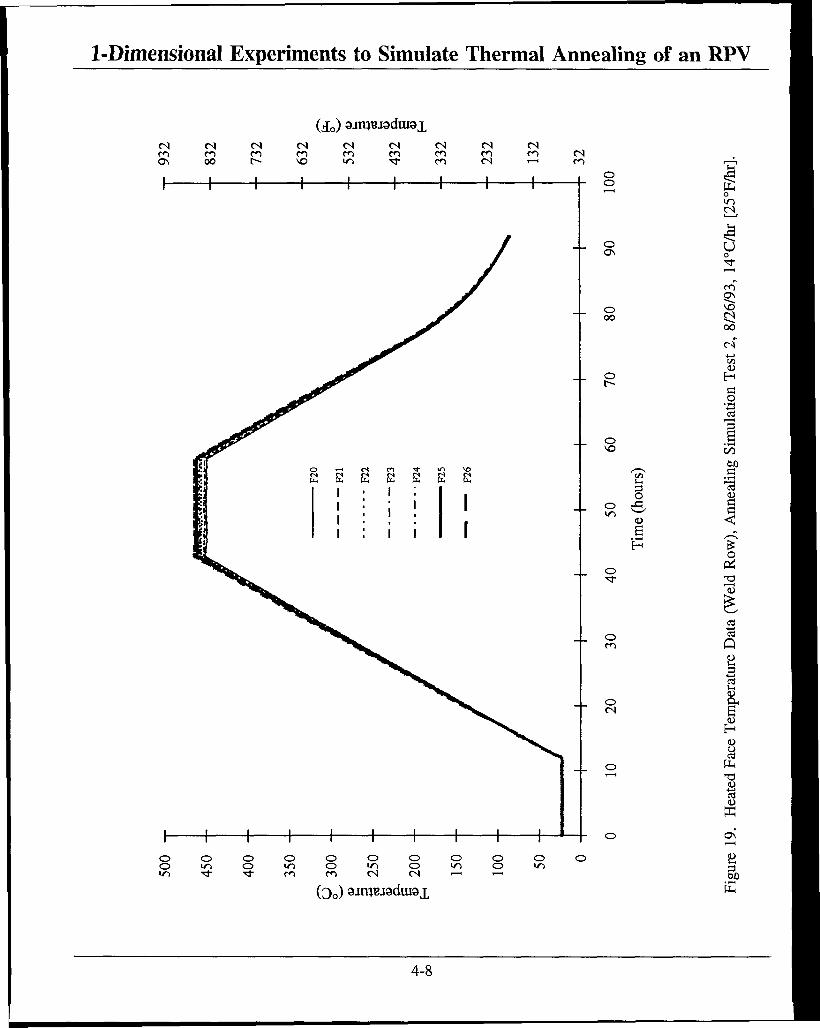
1-Dimensional Experiments to Simulate Thermal Annealing of an RPV
(£ 0) 9irUTU9dtU91 CM CO ON
CM CO oo
CM en r-CM CO vo
CM CO in CO •st-
CM CO CO
CM CO cs CM CO CM
CO o o
o as
o oo
o
o VO
o m
o
o CO
o CM
0>
o
PL, o
>n 1-1
§ CO
vo 00 of
H o 3 CO OJO
a <
o Pi
Q B S3
H (0 o Pi
ON
0 O 0 0 O 0 O O 0 0 0 i n 0 i n O i n O i n 0 i n i n ^ ^ CO CO CM CM <—> > — •
(3 0 ) 9jrm?i9durai 3 bJO
•I—I
ft
4-8

10 20 30 40 50 60
Time (hours)
70 80 90 100
Figure 20. Heated Face Temperature Data (Diagonal), Annealing Simulation Test 2, 8/26/93, 14°C/hr [25°F/hr].

10 20 30 40 50 60
Time (hours)
70 80 90 100
Figure 21. Heated Face Temperature Data (Diagonal), Annealing Simulation Test 2, 8/26/93, 14°C/hr [25°F/hr].

1-DimensionaI Experiments to Simulate Thermal Annealing of an RPV
£ U
C a.
a. a u
+ L 01
r?
C3 oa
(fj
§
(3 -
-20 -10 0 10 • 20 Frorrr Face Tempera+ure Devia+ion from 5e+ Poarrr CO
1 1
Tes+ 2 i
5+ar+ of
1
Soak
1 1 1 0 20 40 60 80 100 120
Hdr jL2on+a l Posx+xon CcrO
Figure 22. Temperature Contour Plot of the Heated Face of the RPV Section at the Beginning of the Soak.
4-11

1-Dimensional Experiments to Simulate Thermal Annealing of an RPV
£ 0
C
+ ••i
IJ1
• U
H 4-L 01
r>
IN
si oa
•<3-
si
a
0
-20 -10 0 10 20 Frorrr Face Tempera+ure Devia+ion from 5e+ Poin+ CO
Tes+ 2 End of Soak
20 40 60 80
Ho' r isan+al P o s i + i o n CcrO
100 120
Figure 23. Temperature Contour Plot of the Heated Face of the RPV Section at the End of the Soak.
4-12
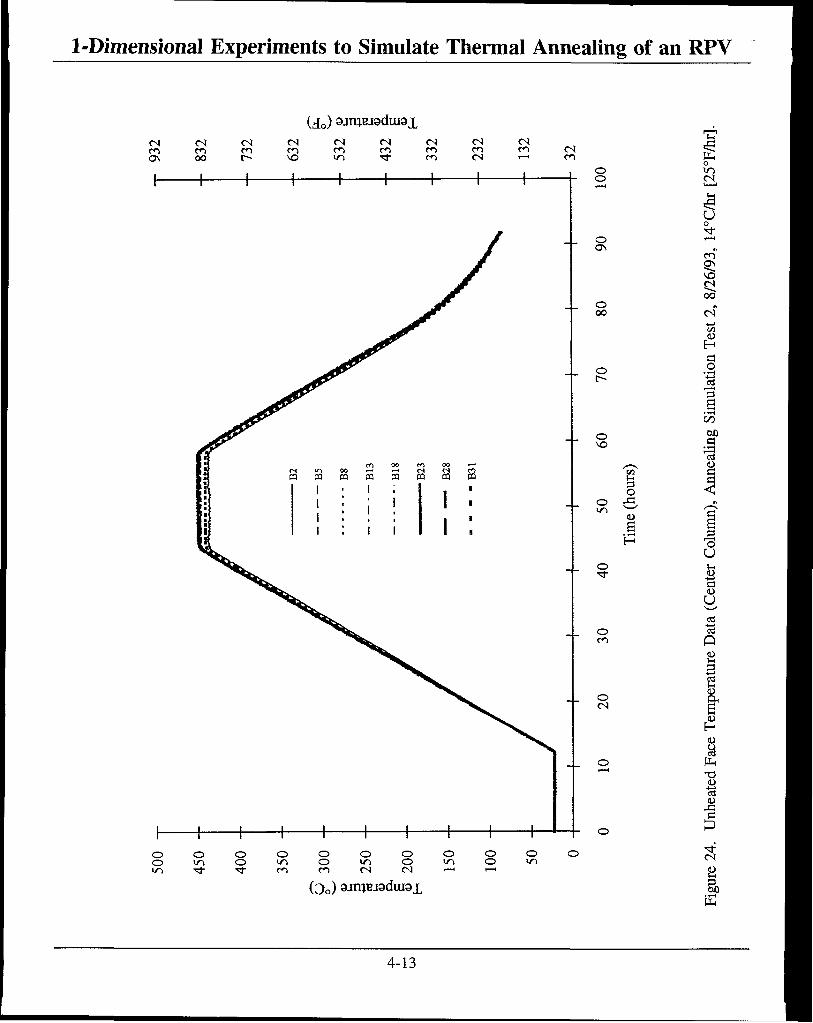
1-Dimensional Experiments to Simulate Thermal Annealing of an RPV
(j 0) sjmujadurax
o o
o o o o o O o o o o o ir> o W) o ir> o i n o IT) Wl rr rr m m CN cs '-* 1 — 1
o m cs
U
o i—l
ON
8/26
/93,
O ^ 0 0
n Te
st 2
O o f -
Sim
ulat
o b0 VO ^
/—"s <u on a
our 5
o J3 ,, «n CD "5* s s H
Col
o u TJ-
ta (
Cent
e
o 03 m
;ratu
re D
o & <N
ace
Tem
O fe
nhea
ted
o
24.
U
( 3 0 ) 9jnjBJ3dui9X P £»0
4-13
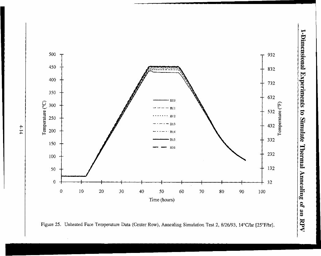
500
10 20 30 40 50 60
Time (hours)
70 80 90
932
832
- - 732
-- 632
-- 532 » fr 3
a , S a> H
100
Figure 25. Unheated Face Temperature Data (Center Row), Annealing Simulation Test 2, 8/26/93, 14°C/hr [25°F/hr].

10 20 30 40 50 60
Time (hours)
70 80 90 100
Figure 26. Unheated Face Temperature Data (Weld Row), Annealing Simulation Test 2, 8/26/93, 14°C/hr [25°F/hr].

102
92
82
52
42
32
10 20 30 40 50 60
Time (hours)
70 80 90 100
PL, O
-- 72 p
2
62 | H
Figure 27. Concrete Wall Temperature Data (Column), Annealing Simulation Test 2, 8/26/93, 14°C/hr [25°F/hr].
3 o 3
W
(73
&5 rl-
H cr
I > 3 sa BS S3
OQ
O
3
<3
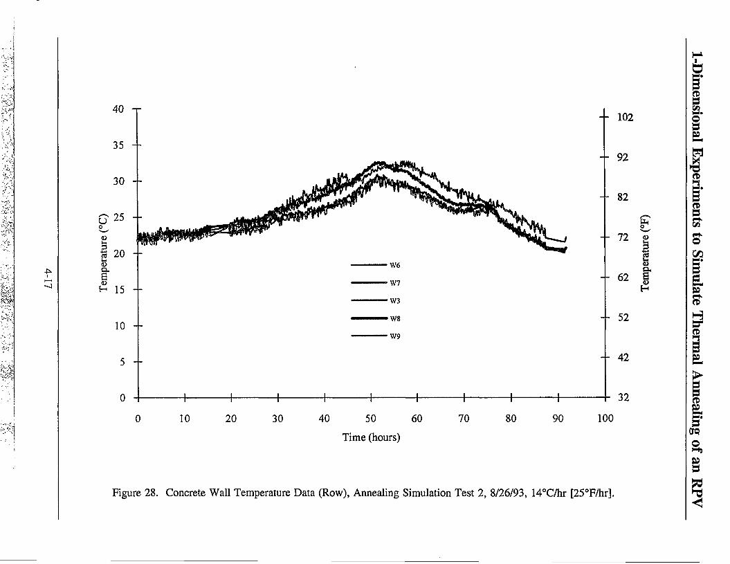
~v;'
§
&;\
m
i i—*
10 20 30 40 50 60 Time (hours)
70 80 90
102
92
-- 82
52
-- 42
32
100
Figure 28. Concrete Wall Temperature Data (Row), Annealing Simulation Test 2, 8/26/93, 14°C/hr [25°F/hr].
& - • 72 P
2
H
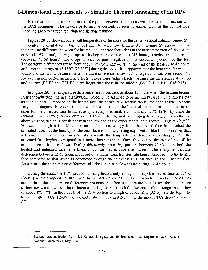
1-Dimensional Experiments to Simulate Thermal Annealing of an RPV Note that the straight line portion of the plots between 16-20 hours was due to a malfunction with
the DAS computer. The heaters performed as desired, as seen by earlier plots of the control TCs. Once the DAS was repaired, data acquisition resumed.
Figures 29-31 show through-wall temperature differences for the center vertical column (Figure 29), the center horizontal row (Figure 30) and the weld row (Figure 31). Figure 29 shows that the temperature difference between the heated and unheated faces rises in the heat-up portion of the heating curve (12-43 hours), sharply drops at the beginning of the soak (43 hours), reaches an equilibrium (between 43-58 hours), and drops to zero or goes negative in the cooldown portion of the test. Temperature differences range from about 12°-23°C [22°-41°F] at the end of the heat-up at 43 hours, and drop to a range of 4°-18°C [7°-32°F] during the soak. It is apparent that the heat transfer was not totally 1-dimensional because the temperature differences show such a large variation. See Section 4.8 for a discussion of 2-dimensional effects. There were "edge effects" because the differences at the top and bottom (F2-B2 and F31-B31) are larger than those in the middle (F8-B8, F13-B13, F18-B18).
In Figure 29, the temperature difference rises from zero at about 12 hours when the heating begins. In heat conduction, the heat distribution "velocity" is assumed to be infinitely large. This implies that as soon as heat is imposed on the heated face, the entire RPV section "feels" the heat, at least to some very small degree. However, in practice, one can estimate the "thermal penetration time," the time it takes for the unheated face to increase by a easily measurable amount, say 1.1 °C [2°F], by using the estimate t = 0.2L 2a (Fourier number = 0.05)3. The thermal penetration time using this method is about 460 sec, which is consistent with the low end of the experimental data shown in Figure 29 (500-700 sec, although it is difficult to see). Therefore, energy from the heated face has reached the unheated face, but the heat-up on the back face is a slowly rising exponential-like function rather than a linearly increasing function [9]. As a result, the temperature difference rises sharply until the unheated face begins to respond in a more linear manner. Once this occurs, the rate of rise of the temperature difference slows. During this slowly increasing portion, between 12-43 hours, both the heated and unheated faces rise linearly, but the heated face rises faster. The rising temperature difference between 12-43 hours is caused by a higher heat transfer rate being absorbed into the heated face compared to that which is conducted through the thickness and lost through the unheated face. As a result, the temperature difference still rises, but at a slower rate during 12-43 hours.
During the soak, the RPV section is being heated only enough to keep the heated face at 454°C [850°F] so the temperature difference drops. After a short time during which the section comes into equilibrium, the temperature differences are constant. Because there are heat losses, the temperature differences are not zero. The differences during the soak period, after equilibrium, range from a low of about 4°C [7°F] in the middle of the RPV section to a high of about 18°C [32°F] near the top. The top and bottom TCs (F2-B2 and F31-B31) show the largest AT, while the middle TCs show the lowest AT.
Personal communication from Ned Keltner, Energetic and Environmental Test Department 2761, Sandia National Laboratories, May 1994.
4-18

25 -r
20 - -
15 --O
o c <- 10
*Q (U
§ <D CL
e <u
H
5 - -
-5
•10
10 20 30 40 50 60
Time (hours) 70 80 90
- - 42
- - 32
22 ^
£
1 H
12
- - -8
-18
100
Figure 29. Through-Wall Temperature Difference (Center Column), Annealing Simulation Test 2, 8/26/93, 14°C/hr [25°F/hr].

1-DimensionaI Experiments to Simulate Thermal Annealing of an RPV
(io) aouarajGFKI amiHioArai t s <s oo
I
0 0
o o
o 00
o
o
o
o
o
o <N
in o m
(Do) 33U9-I9Jffia 3injBJ9dtU9X
o
u o
co
v©
§ of
CO
(U H a o •d
two
1>
CD
s (D
p
2 (D H
I o CO
4-20
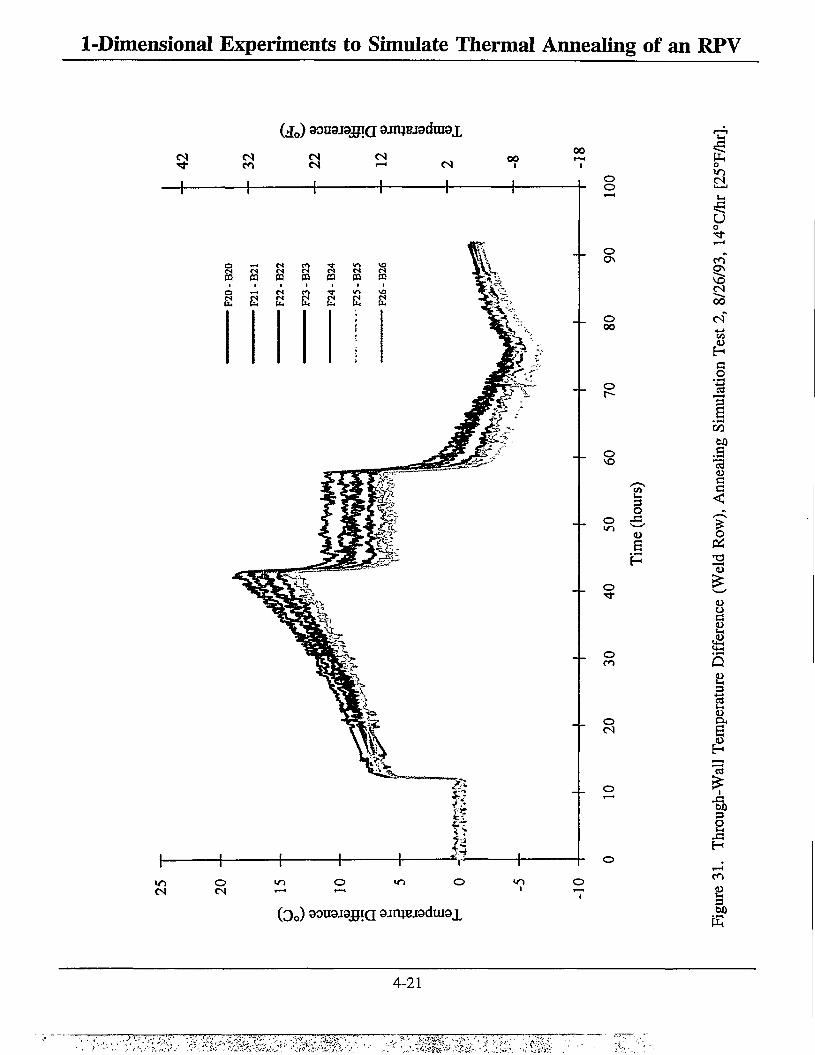
1-Dimensional Experiments to Simulate Thermal Annealing of an RPV
(j 0 ) aousjaj^a ajru&radurax
CO CM CN
cs 00
00
o o
o
o 00
o
o
en t -3 O
O £ , 6 H
o "3-
o CO
o
( 3 Q ) 30U9J3J51Q 9iTUBJ9dtU9X
I o
g o
co ^ \ CN 0 0
of • * - » 1/3 <D H
CS
o So 1
• i-H
co oo a c a
< *
£ <u
o a
.4)
2 s I
J3 00 3 o
en 3 00
4-21
1-Dimensional Experiments to Simulate Thermal Annealing of an RPV During the cooldown portion of the test, heat is no longer being supplied to the heated face. As
a result, both faces of the RPV section begin to cool. Because the previously heated face cools faster, the temperature difference drops quickly and in most locations turns negative. The previously heated face cools faster because it is close to the heaters, which soon drop in temperature, as opposed to the mirror insulation facing the unheated face that reflect heat back to the unheated face as it cools (i.e., the heaters have a lower R-value than the mirror insulation).
Figure 30 shows similar data from the center horizontal row of TCs. The same basic results can be seen except for the lack of high temperature differences seen on the top and bottom in Figure 29. Temperature differences are much more uniform in Figure 30. The plot showing the temperature difference between F10 and BIO shows what is believed to be a poorly mounted thermocouple, one that "pulled" away from the surface of the RPV section during the sudden temperature drop at 43 hours. For example, if the heated face TC pulled off the surface only slightly, so that some thermal contact between the TC and the surface was lost, the TC would read higher than the surface temperature, due to heat input from the heaters. As a result, the temperature difference would rise, as shown. A similar result would occur if unheated face TC pulled off the surface, because it would then read lower than the RPV section temperature and the temperature difference would again rise. Except for the poorly mounted thermocouple, temperature differences range from about 10°-14°C [18°-25°F] at the end of the rise portion at 43 hours, and drop to a range of 2°-5°C [4°-9°F] during the soak.
Figure 31 shows temperature differences from the horizontal weld location row. Similar to Figures 29 and 30, the temperature difference begins at zero, rises sharply as the heat-up begins, sharply changes the slope of the rise after the heat begins to reach the unheated face, drops sharply as the soak begins, reaches an equilibrium during the soak, then drops sharply as the cooldown begins. Temperature differences range from about 14°-19°C [25°-34°F] at the end of the heat-up portion at 43 hours, and drop to a range of 5°-ll°C [9°-20°F] during the soak.
Figures 32 and 33 show temperature differences on the heated and unheated faces, between TCs mounted on the weld and just below the weld on the base metal. The temperature differences on the heated face generally range between ±2°C [±4°F] and on the unheated face between 0° and +2°C [+4°F]. As the heat-up begins, the weld heats up slightly faster than the adjacent base metal temperature, except for TC F21 (Figure 32). The temperature differences slowly drop over time until the soak begins. During the soak the temperature differences are generally constant. At the end of the soak the temperature difference drops to zero or becomes negative. As the RPV section temperature drops, the temperature differences rise again. Because the unheated face temperature differences shown in Figure 33 are always positive, the weld locations temperatures were always slightly above the base metal temperatures. This could be caused by the RPV thickness at the weld being slightly less than the thickness at the adjacent base metal. This would cause a slightly higher temperature at the weld and a positive temperature difference.
4.3.2 Heat Flux Data
Heat flux data are presented from two types of transducers: pyrheliometers and thermocouples. As previously stated, pyrheliometers provide a direct measure of total incident heat flux to the RPV section, while thermocouple data, reduced through SODDIT, provides estimates of total absorbed heat flux. See Section 4.9 for a short discussion regarding uncertainties in heat flux values generated by SODDIT. Figures 34-41 show heat flux data from Test 2.
4-22

10 20 30 40 50 60 Time (hours)
70 80 90 100
Figure 32. Heated Face Temperature Difference (Weld-Base Metal), Annealing Simulation Test 2, 8/26/93, 14°C/hr [25°F/hr].
1-Dimensional Experiments to Simulate Thermal Annealing of an RPV
( £ 0 ) 90U9J9J5IQ 9JtUBJ9dUI9X
ON vO CO en
i VO 0>
i o o
o
o 00
o
o vo
CO
3 O
O <£* <U S H
o
o en
o
o
IT> eo cs —< o •-? CA
( 3 0 ) 90U9J9J5IQ 9JTUBJ9dUJ9X
CO •
i n
o m
u
CO
vo cs oo (N 4-» CO <D H a o
"3 B W) e
13 Hi a c <
CO
ca m i
O
a
Q 3 4-*
2 <D
J3 C
en en
3
E
4-24
1-Dimensional Experiments to Simulate Thermal Annealing of an RPV
Pvrheliometer Data - Incident Heat Flux
Pyrheliometer data are shown in Figure 34. Three (3) pyrheliometers were mounted as shown in Figures 11 and 15. HFl (S/N-930926) was mounted on the vertical centerline between TCs F2 and F5. HF2 (S/N-930927) was mounted left of the vertical centerline, just above TC F l l . HF3 (S/N-930928) was mounted vertically above HF2 and horizontally to the left of HFl, just above TC F4. As can be seen from Figure 34, HFl and HF3 read virtually identical heat flux values, while HF2 is about 25% less. The reason for this difference is due to different power levels consumed by the middle and top heater banks. See Section 4.7.
The heat flux on all three gages rises sharply from zero at about 12 hours up to about 0.34 W/cm [0.30 Btu/ft2-secl. Between 12 and 43 hours the gage outputs rise, but HF2 rises less. HFl and HF3
9 7 1 rise to a maximum of about 2.30 W/cm [2.03 Btu/ft -sec], HF2 to a maximum of about 1.79 W/cm [1.58 Btu/ft -sec]. All three (3) gages show a sharp reduction in flux at 43 hours (beginning of soak) of about 0.37 W/cm 2 [0.33 Btu/ft2-sec]. HFl and HF3, during the soak between 43-58 hours, show a constant heat flux of about 1.93 W/cm2 [1.70 Btu/ft2-sec]. HF2 shows a heat flux of about 1.45 W/cm2 [1.28 Btu/ft2-sec]. After the soak, the heat flux drops off in an exponential like manner.
To estimate the theoretical incident heat flux during the soak, one can perform an energy balance on the heated face (where the pyrheliometers were mounted). The result of such an energy balance is as follows:
q a = ir + q c - qrf^q e P I
where: q i r = radiative heat flux incident on heated face, q a = total heat flux absorbed into heated face, q e = heat flux emitted (i.e., re-radiated) from heated face = ecfP q r f = radiative heat flux reflected from heated face = (1 - a)q i r. q c = convective heat gain on heated face = h(T h - T) a = absorptivity of heated face e = emissivity of heated face a = Stefan-Boltzmann constant: 5.7 x 10" 1 2 W/cm2-°K4 [0.17 x 10"8 Btu/hr-ft2-°R4]
During the soak, the absorbed flux drops to zero, as will be shown below (SODDIT Data -Absorbed Heat Flux). For most diffuse surfaces, the absorptivity and the emissivity are assumed to be equal. This assumption will also be made here, even though the stainless steel cladding may not be a totally diffuse surface (there are limited alternatives that can be made). Upon substitution into equation [2], the following equation results:
q i r = oT 4 - (h/e)(Th - T) [3]
where T is the heated face temperature of the RPV section and T h is the average heater temperature.
4-25

1-Dimensional Experiments to Simulate Thermal Annealing of an RPV
(03S-zy/ma) xntf JB3H u->
e-1 © o o
o ON
IT) <N O
o
o en 00
2, 8
/26/
9
o <i-i
t~-
atio
n Te
o
Sim
u
,—, too a
§ 13 o J3 0)
a 4)
a 5 H C/3
- t-»
o
Pyrh
elio
me
o ^^ rn
Flux
Dat
a O (N
dent
Hea
t
O O
re 3
4. I
n
o a bO
HH
G«»/M) x n H ^9H
4-26
1-Dimensional Experiments to Simulate Thermal Annealing of an RPV The pyrheliometers measure total incident heat flux on the heated face (i.e., radiative plus
convective). Therefore, to estimate the heat flux measured by the pyrheliometers, one needs to know the quantity q i r + q c, obtainable from equation [2]:
%• + % = % + <lif ( w h e n % = °) M = e&T4 + (l-£)q i r [5]
Using the result of equation [3]:
q i r + q c = oT 4 + h(T h - T)[l-l/e] [6]
Assuming the average temperature of the RPV section was 454°C [850°F], the surface emissivity is e = 0.85, the Nusselt number (hd/k) is 8.384 (therefore h = 1.71 x 10"4 W/cm2-°C [0.30 Btu/ft2-hr-°F]) and the maximum difference between the RPV section and heater temperature is 119°C [215°F]. The term containing the convective component on the right side of equation [6] is very small compared with the first term. Therefore, the total incident heat flux as measured by the pyrheliometers can be approximated as:
q i r + q c = a T 4 = 1.59 W/cm2 [1.40 Btu/ft2-sec] [7]
This theoretical value is between the values measured by the pyrheliometers: 1.93 W/cm [1.70 Btu/ft -sec] (HFl and HF3) and 1.45 W/cm2 [1.28 Btu/ft2-sec] (HF2). The measured values from HFl and HF3 were about 21% above the theoretical value, while the measured value from HF2 was about 9% below the theoretical value. Because both HFl and HF3 read the same but HF2 read lower, one might expect the output from the top heater bank was more than that from the middle heater bank, and this was the case.
The input electrical energy (kW) into each bank of three heaters was recorded for each test. That data showed the bottom bank of heaters consumed the most power because the bottom bank faced the mounting structure, which absorbed a considerable amount of additional energy. The top bank of heaters consumed more electrical energy than the middle bank but less than the bottom bank. The middle bank consumed the least amount of energy. As a result, the incident heat flux output from the top pyrheliometers (HFl and HF3) should have been higher than that from the middle pyrheliometer (HF2), agreeing with the measurements. See Section 4.7 for a more detailed discussion of the power input to the heaters.
One may question, for differing levels of incident heat flux on the top part of the RPV section (HFl and HF3) as compared to the middle (HF2), why the RPV section temperatures are the same: 454°C [850°F]. The reason has to do with 2-dimensional heat transfer and "edge effects." Although these experiments were predominantly 1-dimensional, because of the non-uniform heated face temperatures, there was some 2-dimensional heat transfer. This (2-dimensional heat transfer) required increased heat flux to effect 454°C [850°F] at the top of the RPV section as compared with the center. The top part of the RPV had a net heat loss and therefore required more than the theoretical value,
Personal communication between Walt Gill, Sandia National Laboratories, and Jim Nakos, August 25, 1994. Assumes a heater temperature of 574°C [1065°F] and RPV section temperature of 454°C [850°F] and uses correlation 7-31 for free convection in an enclosed space between vertical walls from Kreith [14].
4-27
1-Dimensional Experiments to Simulate Thermal Annealing of an RPV while the center had a net heat gain, so required less than the theoretical value. See Section 4.8 for further discussion of 2-dimensional effects.
As noted above, the heat flux measured by all pyrheliometers dropped sharply at the beginning of the soak. The magnitude of the drop was about 0.38 W/cm2 [0.33 Btu/ft2-sec]. Because the absorbed heat flux drops to zero during the soak, the magnitude of the drop indicated by the pyrheliometers should be the same as the magnitude of the absorbed flux estimated by SODDIT just before the soak began. As will be seen from the absorbed heat flux data that follows, the maximum amount of heat flux absorbed into the RPV section just before the beginning of the soak was about 0.32 W/cm2 [0.28 Btu/ft2-sec], 13.5% less than the value given above (0.38 W/cm2 [0.33 Btu/ft2-sec]). (These two values should be equal.)
SODDIT Data - Absorbed Heat Flux
Figures 35-37 show absorbed data generated from heated face TCs. Figures 38-40 show heat flux data generated from unheated face TCs. Figure 41 shows the difference between the heat flux generated from heated face TC F3 and unheated face TC B3.
Figures 35-37 show absorbed heat flux on the heated face from heated face TCs. All plots have the same basic shape with slightly different magnitudes. The absorbed heat flux rises sharply from zero to about 0.25 W/cm2 [0.22 Btu/ft2-sec] then rises slowly up to about 0.32 W/cm2 [0.28 Btu/ft2-sec]. The initial step up to 0.25 W/cm2 [0.22 Btu/ft2-sec] compares favorably with the predicted values from Section 3.2 (0.24 W/cm2 [0.21 Btu/ft2-sec]). The predicted value of absorbed flux is constant, while the actual value slowly increases to 0.32 W/cm2 [0.28 Btu/ft2-sec]. This was due to the adiabatic boundary condition assumption used on the back side when calculating predicted values, which was not the case during the test. Because there was finite heat loss from the unheated face by conduction and radiation, the absorbed flux constantly rose slowly throughout the heat-up.
As soon as the soak began, the absorbed flux dropped sharply and eventually reached zero. This would be expected because the temperature of the RPV section is constant and the net absorbed flux should be zero. (See the discussion of equation [2] above). The absorbed flux continued at zero until the cooldown portion began, when the absorbed flux went sharply negative, indicating a net heat loss from the RPV section. As the temperature of the RPV section slowly dropped to ambient, the absorbed flux rose towards zero due to a decreasing rate of heat loss.
Absorbed heat flux on the heated face from unheated face TCs are shown in Figures 38-40. The major differences in flux values generated between the heated and unheated faces are due to noise content and time lag. The same basic shape and magnitudes shown in Figures 35-37 are repeated in Figures 38-40. However, as can be seen in Figure 39, the curves are "noisier." This was unexpected. The test plan indicated absorbed heat flux generated from heated face TCs would likely be noisier because it would be more affected by minor changes in the heated face temperature. However, this was not the case. Absorbed flux from unheated face TCs proved to be noisier, due to SODDIT amplifying small variations in TC output into larger variations in predicted absorbed flux. A 1°C [2°F] variation in temperature on the heated face would cause a smaller change in heat flux than would the same temperature change on the unheated face. Inverse heat conduction codes (e.g., SODDIT) are sensitive to noise. Figure 40 shows "smoothed" output from TC B2, and as one would expect, the
4-28

0.4
0.3
0.2
§ 0.1
KS
X
I -0.1
-0.2
-0.3 - -
-0.4
-r 0.35
0.25
-- 0.15
- - 0.05
SO I
a X
-0.05 E
0.15
-0.25
-1- -0.35
Time (hours)
Figure 35. Absorbed Heat Flux Data Using SODDIT (Heated Face Thermocouples), Annealing Simulation 2, 8/26/93, 14°C/hr [25°F/hr].

0.4
0.3
0.2
§ 0.1
c5
£ o
1 -0.1
-0.2
-0.3
-0.4
0.35
-0.35
Time (hours)
Figure 36. Absorbed Heat Flux Data Using SODDIT (Heated Face Thermocouples-Center Row), Annealing Simulation 2, 8/26/93, 14°C/hr [25°F/hr].

0.4 -r
0.3 - -
0.2 - -
§ 0.1
t 0 X
I -0.1
-0.2 - -
-0.3
-0.4
0.35
0.25
-- 0.15
0.05 h
-0.05 E
in
0.15
-0.25
-L -0.35
Time (hours)
Figure 37. Absorbed Heat Flux Data Using SODDIT (Heated Face Thermocouples - Bottom Row), Annealing Simulation 2, 8/26/93, 14°C/hr [25°F/hr].

0.4
0.3
0.2
0.1 --
0.1
0.2
0.3
0.4
0.35
-- 0.25
0.15
-- 0.05
t/j
£5
¥ -0.05 E
-0.15
-0.25
-0.35
Time (hours)
Figure 38. Absorbed Heat Flux Data Using SODDIT (Unheated Face Thermocouples), Annealing Simulation 2, 8/26/93, 14°C/hr [25°F/hr].

1-Dimensional Experiments to Simulate Thermal Annealing of an RPV
(s-zwma) x n u *B9H IT) CO
IT)
o o o
U0 o o
I ©'
I
IT) co
3 O
s
o CO
o
_L o
o o a t/3 S P
I « 3 O
<D
o
o m CN
a CO 0 \
• \D CS oo
§ 00
cs o
Q
3
s=S • I—I
5 3
•8 o en
ON
8 3
O CO O O o
CO
o" o
yao/sm/A) x n I 4 JB3H
4-33
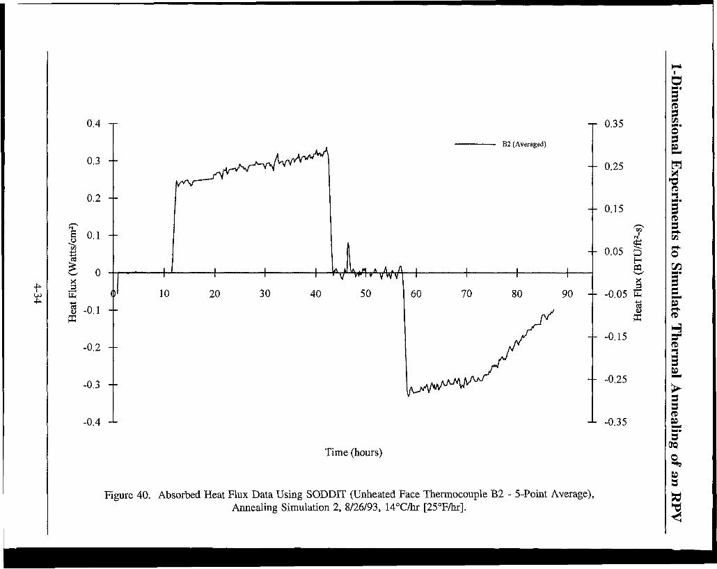
-r 0.35
0.25
-- 0.15
0.05
'en i
B ffl. 5
-0.05 E
-0.15
-0.25
-1- -0.35
Time (hours)
Figure 40. Absorbed Heat Flux Data Using SODDIT (Unheated Face Thermocouple B2 - 5-Point Average), Annealing Simulation 2, 8/26/93, 14°C/hr [25°F/hr].
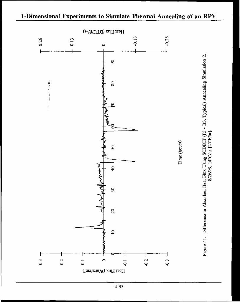
1-Dimensional Experiments to Simulate Thermal Annealing of an RPV
(s-zwnie) ™u ww CO
o
CO
O o
§
s
a o
on 60 a
-3 o a,
en" PQ
en
o
P P O
en i—1
^ en
E fN c3
I o C/i
3 O a
i E
OO
en O
cs o o
en O
(zuio/swBAv) xnij ;BSH
4-35
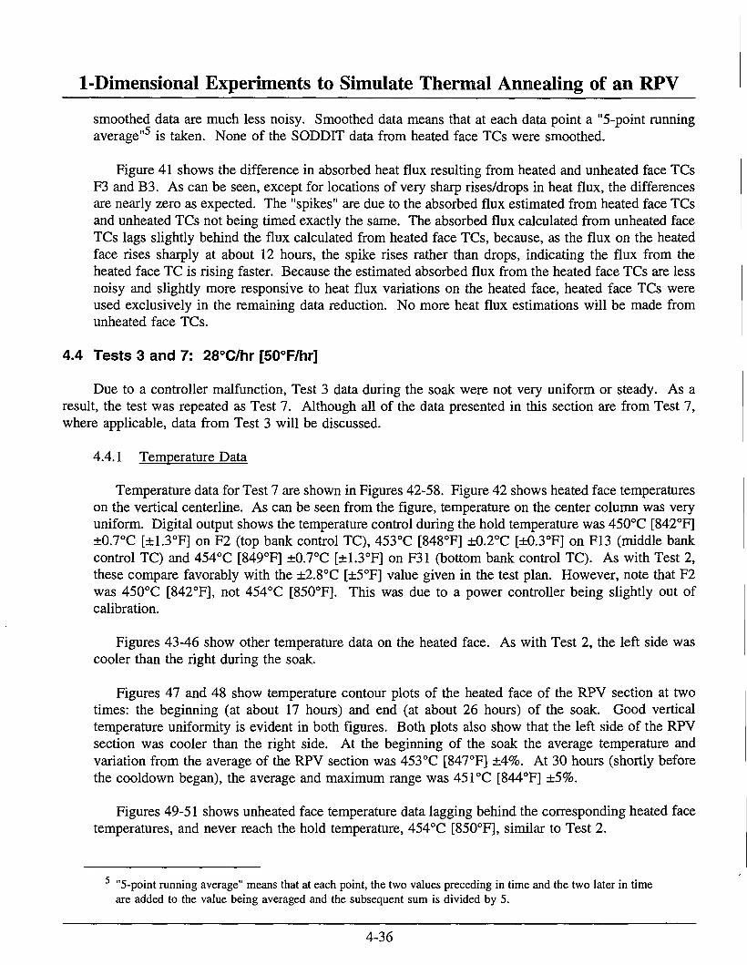
1-Dimensional Experiments to Simulate Thermal Annealing of an RPV smoothed data are much less noisy. Smoothed data means that at each data point a "5-point running average"5 is taken. None of the SODDIT data from heated face TCs were smoothed.
Figure 41 shows the difference in absorbed heat flux resulting from heated and unheated face TCs F3 and B3. As can be seen, except for locations of very sharp rises/drops in heat flux, the differences are nearly zero as expected. The "spikes" are due to the absorbed flux estimated from heated face TCs and unheated TCs not being timed exactly the same. The absorbed flux calculated from unheated face TCs lags slightly behind the flux calculated from heated face TCs, because, as the flux on the heated face rises sharply at about 12 hours, the spike rises rather than drops, indicating the flux from the heated face TC is rising faster. Because the estimated absorbed flux from the heated face TCs are less noisy and slightly more responsive to heat flux variations on the heated face, heated face TCs were used exclusively in the remaining data reduction. No more heat flux estimations will be made from unheated face TCs.
4.4 Tests 3 and 7: 28°C/hr [50°F/hr]
Due to a controller malfunction, Test 3 data during the soak were not very uniform or steady. As a result, the test was repeated as Test 7. Although all of the data presented in this section are from Test 7, where applicable, data from Test 3 will be discussed.
4.4.1 Temperature Data
Temperature data for Test 7 are shown in Figures 42-58. Figure 42 shows heated face temperatures on the vertical centerline. As can be seen from the figure, temperature on the center column was very uniform. Digital output shows the temperature control during the hold temperature was 450°C [842°F] ±0.7°C [±1.3°F] on F2 (top bank control TC), 453°C [848°F] ±0.2°C [±0.3°F] on F13 (middle bank control TC) and 454°C [849°F] ±0.7°C [±1.3°F] on F31 (bottom bank control TC). As with Test 2, these compare favorably with the ±2.8°C [±5°F] value given in the test plan. However, note that F2 was 450°C [842°F], not 454°C [850°F]. This was due to a power controller being slightly out of calibration.
Figures 43-46 show other temperature data on the heated face. As with Test 2, the left side was cooler than the right during the soak.
Figures 47 and 48 show temperature contour plots of the heated face of the RPV section at two times: the beginning (at about 17 hours) and end (at about 26 hours) of the soak. Good vertical temperature uniformity is evident in both figures. Both plots also show that the left side of the RPV section was cooler than the right side. At the beginning of the soak the average temperature and variation from the average of the RPV section was 453°C [847°F] ±4%. At 30 hours (shortly before the cooldown began), the average and maximum range was 451°C [844°F] ±5%.
Figures 49-51 shows unheated face temperature data lagging behind the corresponding heated face temperatures, and never reach the hold temperature, 454°C [850°F], similar to Test 2.
"5-point running average" means that at each point, the two values preceding in time and the two later in time are added to the value being averaged and the subsequent sum is divided by 5.
4-36
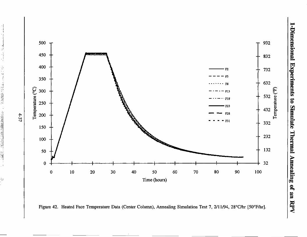
0 10 20 30 40 50 60 Time (hours)
70 80 90
-r 932
- - 832
- - 732
-- 632
532 £ i & 432 g. H
- - 332
- - 232
132
32
100
Figure 42. Heated Face Temperature Data (Center Column), Annealing Simulation Test 7, 2/11/94, 28°C/hr [50°F/hr].
500 932
0 10 20 30 40 50 60
Time (hours)
70 80 90 100
Figure 43. Heated Face Temperature Data (Center Row), Annealing Simulation Test 7, 2/11/94, 28°C/hr [50°F/hr].
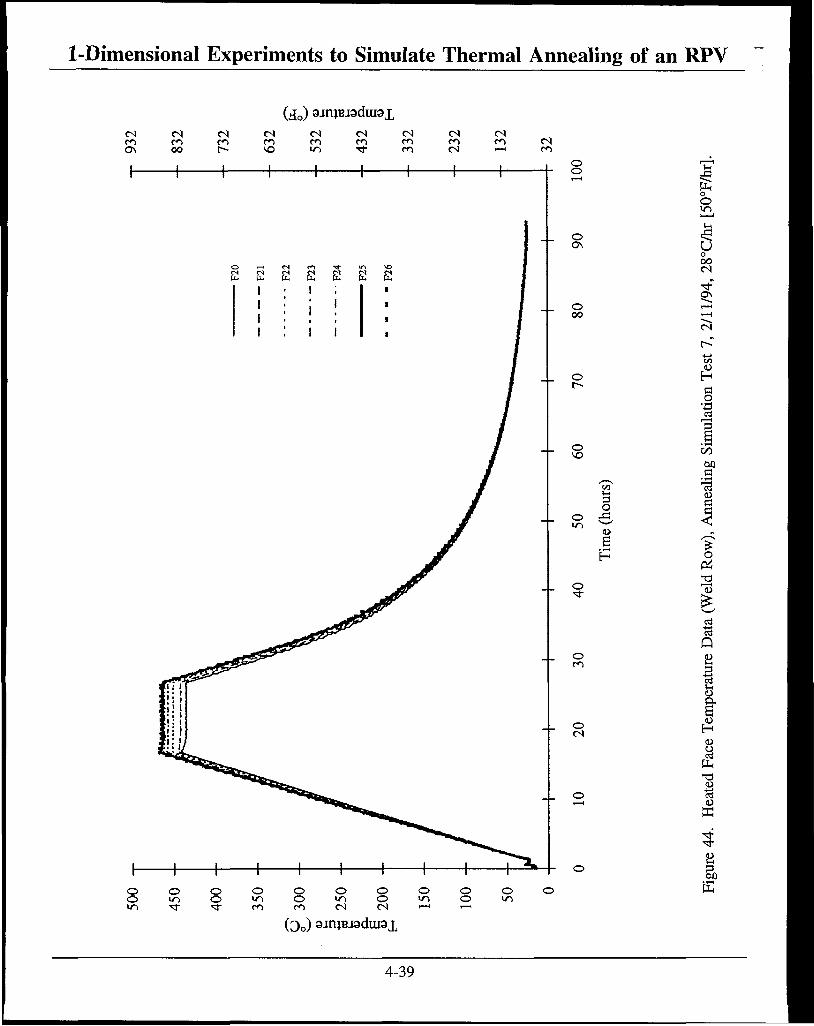
1-DimensionaI Experiments to Simulate Thermal Annealing of an RPV
( j 0 ) 9JmtU9dU»l
o o
o 0\
O 00
o c--
P-, o O
u o oo <N
<N
H o
•a
o
ingS
i
02 13
o (hou
r
Ann
e
4> „ a £ H
dRo
o •"3-
Dat
a (W
<
o D m
mpe
ratu
r O
ted
Face
Te
o a
re 4
4. H
e
o a t>0 o o 8 o O O O o o o
o m 8 IT) © IT) O »/"> o ir> »T) • * •* CO m <N <s 1—1 '-'
fc
( 3 0 ) 9jnjBJ9dui9i
4-39
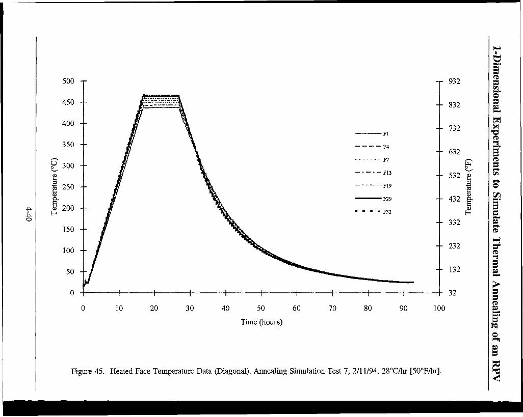
0 10 20 30 40 50 60
Time (hours)
70 80 90 100
Figure 45. Heated Face Temperature Data (Diagonal), Annealing Simulation Test 7, 2/11/94, 28°C/hr [50°F/hr].

1-Dimensional Experiments to Simulate Thermal Annealing of an RPV
(40) sjraejsduiai
oo r- co CS en <N CO
£ £ F13 r- r-
E 2 F30
I 1 I 1
1
1
1
1
1
•
• •
o o
o ON
o oo
o
o
o
©
o
O
3 O
s
o
o o o © o o o o o o © i n o wo o U 1 o <o o »r> «n TT •sr C I m CM cs r - H « — '
o O
o oo <N
<N
H a o s 1 i/3 00 a 13 a
<
c o oo
S
Q B 3
H D
i
3 00
( 3 0 ) 9jnjBJ9dui3i
4-41

1-Dimensional Experiments to Simulate Thermal Annealing of an RPV
IN
•H £ U
^_i r?. C UJ
u • H
+ •-i
a 63 m LL
H n ii -i N + r-t-
M i. 01 >
ra IM
a
-20 -10 B 10 20 Frarrf Face Tempera+ure Devia+ion from 5e+ Poj.rrr CC""i
feS'.«Ife
Tesf ? 5+ar+ of Soak
40 60 0 20 80 100 120 H o r i s o n + a l P o s i + i o n Ccm"
Figure 47. Temperature Contour Plots of the Heated Face of the RPV Section at the Beginning of the Seal.
4-42

1-Dimensional Experiments to Simulate Thermal Annealing of an RPV
CJ
c
• U H + £-•
fM
(3 ca
U3
(3 -
-20 -le 0 10 20 Frorrr Face Temper a+ure Devia+ion from 5e+ Poj.n+ C O
Tes+ 7 End of 5oak
~~1 1 1 — 40 60 80 H o r i ^ o n + a l P o s i + i o n CcrO
0 20 100 120
Figure 48. Temperature Contour Plots of the Heated Face of the RPV Section at the End of the Seal.
4-43
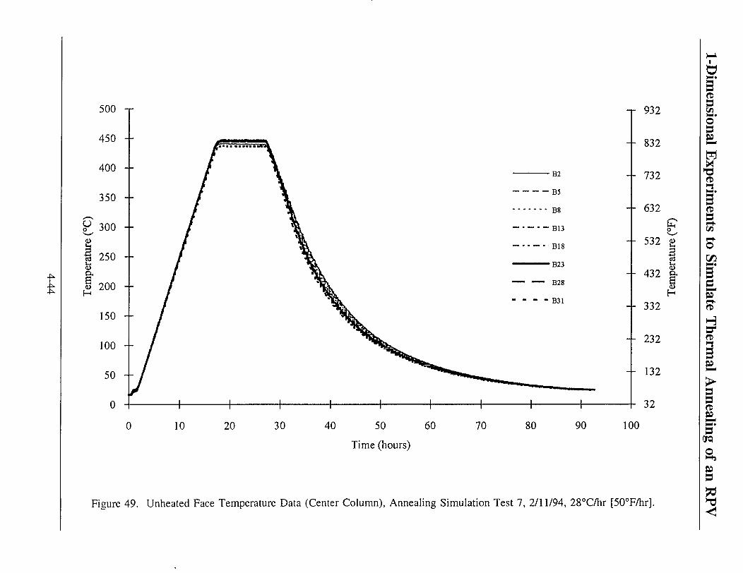
10 20 30 40 50 60
Time (hours)
70 80 90 100
Figure 49. Unheated Face Temperature Data (Center Column), Annealing Simulation Test 7, 2/11/94, 28°C/hr [50°F/hr].
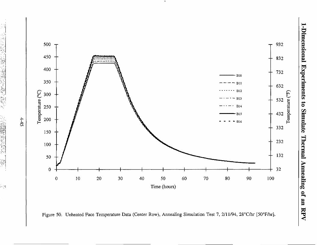
i
\--'i
•:,'>A
4^
0 10 20 30 40 50 60
Time (hours)
70 80 90 100
Figure 50. Unheated Face Temperature Data (Center Row), Annealing Simulation Test 7, 2/11/94, 28°C/hr [50°F/hr].
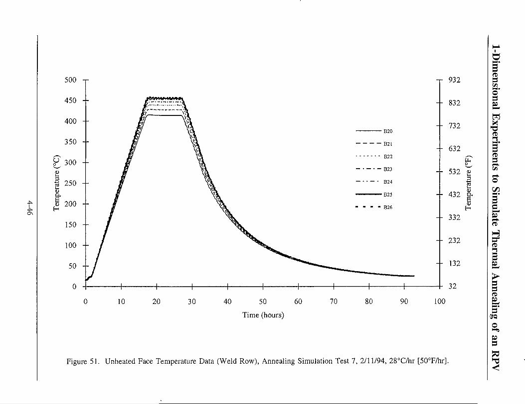
10 20 30 40 50 60
Time (hours)
70 80 90 100
Figure 51. Unheated Face Temperature Data (Weld Row), Annealing Simulation Test 7, 2/11/94, 28°C/hr [50°F/hr].
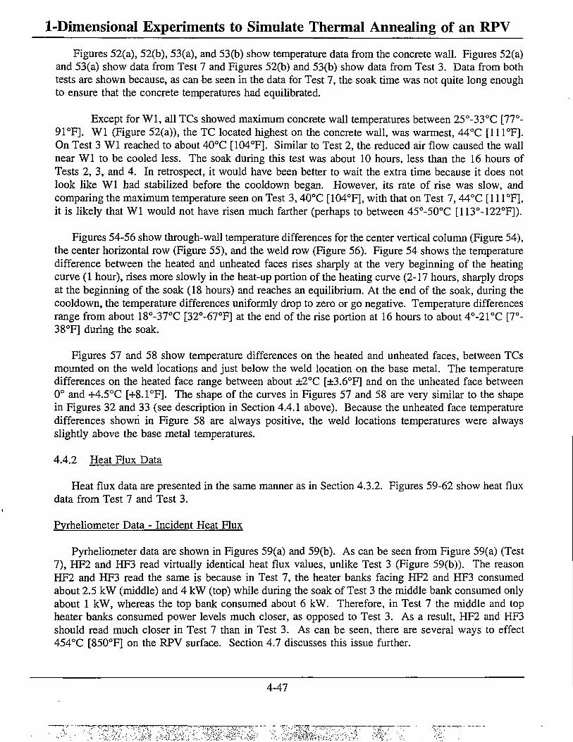
1-Dimensional Experiments to Simulate Thermal Annealing of an RPV Figures 52(a), 52(b), 53(a), and 53(b) show temperature data from the concrete wall. Figures 52(a)
and 53(a) show data from Test 7 and Figures 52(b) and 53(b) show data from Test 3. Data from both tests are shown because, as can be seen in the data for Test 7, the soak time was not quite long enough to ensure that the concrete temperatures had equilibrated.
Except for Wl, all TCs showed maximum concrete wall temperatures between 25°-33°C [77°-91°F]. Wl (Figure 52(a)), the TC located highest on the concrete wall, was warmest, 44°C [111°F]. On Test 3 Wl reached to about 40°C [104°F]. Similar to Test 2, the reduced air flow caused the wall near Wl to be cooled less. The soak during this test was about 10 hours, less than the 16 hours of Tests 2, 3, and 4. In retrospect, it would have been better to wait the extra time because it does not look like Wl had stabilized before the cooldown began. However, its rate of rise was slow, and comparing the maximum temperature seen on Test 3,40°C [104°F], with that on Test 7,44°C [111°F], it is likely that Wl would not have risen much farther (perhaps to between 45°-50°C [113°-122°F]).
Figures 54-56 show through-wall temperature differences for the center vertical column (Figure 54), the center horizontal row (Figure 55), and the weld row (Figure 56). Figure 54 shows the temperature difference between the heated and unheated faces rises sharply at the very beginning of the heating curve (1 hour), rises more slowly in the heat-up portion of the heating curve (2-17 hours, sharply drops at the beginning of the soak (18 hours) and reaches an equilibrium. At the end of the soak, during the cooldown, the temperature differences uniformly drop to zero or go negative. Temperature differences range from about 18°-37°C [32°-67°F] at the end of the rise portion at 16 hours to about 4°-21°C [7°-38°F] during the soak.
Figures 57 and 58 show temperature differences on the heated and unheated faces, between TCs mounted on the weld locations and just below the weld location on the base metal. The temperature differences on the heated face range between about ±2°C [±3.6°F] and on the unheated face between 0° and +4.5°C [+8.1°F]. The shape of the curves in Figures 57 and 58 are very similar to the shape in Figures 32 and 33 (see description in Section 4.4.1 above). Because the unheated face temperature differences shown in Figure 58 are always positive, the weld locations temperatures were always slightly above the base metal temperatures.
4.4.2 Heat Flux Data
Heat flux data are presented in the same manner as in Section 4.3.2. Figures 59-62 show heat flux data from Test 7 and Test 3.
Pyrheliometer Data - Incident Heat Flux
Pyrheliometer data are shown in Figures 59(a) and 59(b). As can be seen from Figure 59(a) (Test 7), HF2 and HF3 read virtually identical heat flux values, unlike Test 3 (Figure 59(b)). The reason HF2 and HF3 read the same is because in Test 7, the heater banks facing HF2 and HF3 consumed about 2.5 kW (middle) and 4 kW (top) while during the soak of Test 3 the middle bank consumed only about 1 kW, whereas the top bank consumed about 6 kW. Therefore, in Test 7 the middle and top heater banks consumed power levels much closer, as opposed to Test 3. As a result, HF2 and HF3 should read much closer in Test 7 than in Test 3. As can be seen, there are several ways to effect 454°C [850°F] on the RPV surface. Section 4.7 discusses this issue further.
4-47

1-Dimensional Experiments to Simulate Thermal Annealing of an RPV
( j 0 ) 9jr4BJ9dUJ9X CN CN
o CN CN 1 — < ON oo
CN CN <N i n
CN CN
O O
O ON
O 00
o
o NO
o m
o
o
o CN
3 O
£
in o in o in O • * TT m c-> <N CN
o O m
6 o oo CN
O N
CN
r-* CO CD
H G O
3
s 00 c
• H
G G < G
s 3 O U ctf
Q
CO
e H
<L) -4—»
(U u, O G O U
of i n 4J u. 3 00
E ( 3 Q ) 9JnjBJ9dUJ9I
4-48

1-DimensionaI Experiments to Simulate Thermal Annealing of an RPV
(£0) ajruuisduisi cs <s
o CS 00 CS CS CS in
cs CS C")
O
o
O m
o 3 O
P O
O CS
in o >n CO in cs in
s o O m i — i
u o 00 CS ON
CS en"
• * - *
a o • 4 — »
a 00 M C <u G C < c 6 _3 "o U a • 4 — »
Q 3
6
ca
§ c o U cs >n 3 bO
(3 0) ajruuradurai
4-49
cs cs

1-Dimensional Experiments to Simulate Thermal Annealing of an RPV
( £ 0 ) 3imBJ3dUI31 C-4 <N
O <N cs ( S C-4 cs (N ON 00 t-- VO i n •st-
<N O O
O
O CO
O r-i
PH o O
U o oo (N ON
<N
co ID
o H r-
imul
atio
n
o 00 o 00
G GO 13 L- <u 3 G O C o
in ^ < <D /*->* C £
H
a(Ro
o • = 1 -
eratu
re D
at
o a. c,
Tem
a
a) l - c
o G O U en iri <u u. 3 00
in o CN <N O 0 ) ajnjejadurai
4-50

45 -r
40
35 --
30 --O ^ 2 5 + I | 20
H
15 --
10 --
5 --
0 0
' W6
• W7
'W3
•W8
'W9
112
102
92
82
72
62
-- 52
-- 42
32
10 20 30 40 Time (hours)
50 60 70
1 Si w H
Figure 53(b). Concrete Wall Temperature Data (Row), Annealing Simulation Test 3, 2/11/94, 28°C/hr [50°F/hr].

to
10 20 30 40 50 Time (hours)
60 70 80 90 100
Figure 54. Through-Wall Temperature Difference (Center Column), Annealing Simulation Test 7, 2/11/94, 28°C/hr [50°F/hr].

O 25 <a o a <u
i Q
cti u. <D Ou B H
10 20 30 40 50 60 Time (hours)
70 80 90
72
62
52
-- 42 fr o G £ 3 2 s Q S i-.
t <u
H
22
12
-8
-18
100
Figure 55. Through-Wall Temperature Difference (Center Row), Annealing Simulation Test 7, 2/11/94, 28°C/hr [50°F/hr].

1-Dimensional Experiments to Simulate Thermal Annealing of an RPV
(io) 33U9J9_JJ!CI 9JniBJ9dui9X
"3- -3-<N VO — <N
O o
o o
o ON
o oo
o
o o
u. 3 O
o
o
o
o o
(J0) 93U9J9yiQ 9Jn}BJ9dU!9X
r j
o O
U o oo
ON
(N
r-* • * — » (/> <D
H a o
3 6
S3 60 C
1 3 <u c c
<
o
-a
o c l - c
3 4—»
u.
s
C3
J3 00 3 O u<
-C H
3 00
4-54

1-Dimensional Experiments to Simulate Thermal Annealing of an RPV
(j 0) aouajajjiQ ajniBjaduiax "3-00 o"
vo vo
•F27
•F28
•F29
F21
F23
F25
o o
o as
o oo
o
o SO
s
o
o c«1
O
ur> CS <N
(JQ) 90U3J9jgtia 9jrUBJ9dUI3X
£ o O in
U o 00 CO
H c o
• f — »
4-*
00 00 a D C G <
-t-»
o c3
I
<L> O C
a
u, 3 -t-» c3 i~> (D I H <u o
UH * 0
>n
3 00
4-55

1-Dimensional Experiments to Simulate Thermal Annealing of an RPV
(do) 99U9J9jgiQ 3injBJ9dui9X
0 0 NO Tits' o
NO NO CO I
-B27
-B28
-B29
B21
B23
B25
o o
o ON
o 00
o t--
o NO
o
o
o
r o CS i—' o
(Do) 93U9-I9JJICI 9JtlJBJ9dlU9X
<S
o O in
U o oo cs Tj-" ON
l> -t-> C/3 <D
H (3 O
• <—i 00 00 c
15
l - l OS
o (hou
Met
<o OJ
a cd H
ld-B
o !> •sr £ 1) o «
1
H <u o a
•a oo
bO
4-56

1-Dimensional Experiments to Simulate Thermal Annealing of an RPV
(03s-ry/nxe) ™ld JBSH
i n <N ©
o o
o
o 00
o
o VO
o >n
o
o m
o
1
o
en «n cs «n o
o O in
U o oo xt-"
c*
c/3
H a o •a i — c i 00 a
I I o •s Si •a Q X 3
<u
a (D
'o a
m 3 00
(ZUI3/AV) xnj j JB3H
4-57
1-Dimensional Experiments to Simulate Thermal Annealing of an RPV
(33s- zuynia) xntf V&H i n
CN O
•r- CM CO U . UL U . X X X
o O
O
O oo
o f -
o SO
o
o
o en
O CN
3 O
E
CN CN ©'
o O
U o oo CN • * "
O N
<N
en -4-t
<D
E -c o
a 00
a
<u e e
< 00
•s a
-4_-»
Q x 3
E
4—* C <u O c
m a 3 GO
ku»/M) x n l £ Iran
4-58
1-Dimensional Experiments to Simulate Thermal Annealing of an RPV In Test 7 (Figure 59(a)) the heat flux on HF2 and HF3 rose sharply from zero at about 1 hour up
to about 0.50-0.60 W/cm2 [0.44-0.53 Btu/ft2-sec]. Between 1 and 16 hours the gage outputs rise; HF2 and HF3 reach maxima of about 2.30 W/cm2 [2.02 Btu/ft2-sec]. During the soak between 17-26 hours, both gages show a heat flux of about 1.57 W/cm2 [1.38 Btu/ft2-sec], which compares favorably with the values calculated earlier: 1.59 W/cm2 [1.40 Btu/ft2-sec] (see Section 4.3.2). The heat flux drops off in an exponential like manner at the end of the soak. Both gages show a sharp reduction in flux at 17 hours of about 0.70 W/cm2 [0.63 Btu/ft2-sec]. As will be seen below, the estimated absorbed flux from SODDIT just before the soak begins averages about 0.62 W/cm2 [0.55 Btu/ft2-sec], 12.7% less than 0.70 W/cm2 [0.63 Btu/ft2-sec].
In Test 3, the heat flux measured by pyrheliometers HF1 and HF3 rose sharply from zero to about 0.50-0.60 W/cm2 [0.44-0.53 Btu/ft2-sec]. Between 1 and 16 hours HF1 and HF3 rose in tandem while HF2 rose more slowly, similar to Test 2. The maxima reached on HF1 was 2.63 W/cm2 [2.31 Btu/ft2-sec], on HF3 was 2.53 W/cm2 [2.23 Btu/ft2-sec], while HF2 only reached 2.24 W/cm2 [1.97 Btu/ft2-sec]. During the soak, HF1 and HF3 dropped to about 1.96 W/cm2 [1.73 Btu-ft2-sec] while HF2 dropped to 1.50 W/cm [1.32 Btu/ft -sec]. These values span the predicted nominal value of 1.59 W/cm2 [1.40 Btu/ft2-sec].
As the soak begins, HF1 drops by about 0.67 W/cm2 [0.59 Btu/ft2-sec], HF2 by 0.57 W/cm2 [0.50 Btu/ft2-sec] and HF3 by about 0.74 W/cm2 [0.65 Btu/ft2-sec]. These also compare favorably with the drop in absorbed heat flux of 0.62 W/cm2 [0.55 Btu/ft2-sec].
One may question why HF2 and HF3 read virtually the same on Test 7 (Figure 59(a)) but very different in Test 3 (Figure 59(b)) for the same heat-up rate. This is due to a smaller 2-dimensional effect in Test 7 as compared to Test 3. Figures 47 and 48 show heated face temperature contours for Test 7; it can be seen that on the left side of the RPV section (where HF2 and HF3 are located) there is a vertical strip (of green) where the temperature is within a 10°C [18°F] band. This is in contrast to Test 3 (not shown) and Test 2 (Figures 22 and 23). As a result, the 2-dimensional effect on Test 7 is less as compared to Test 3 and Test 2, so incident fluxes on HF2 and HF3 should measure closer values.
SODDIT Data - Absorbed Heat Flux
Figures 60-62 show absorbed data generated from heated face TCs. As stated above, no absorbed heat flux estimations were made using unheated face TCs. All plots have the same basic shape with slightly different magnitudes and are very similar to Test 2. The absorbed heat flux rises sharply from zero to between 0.4-0.5 W/cm2 [0.35-0.44 Btu/ft2-sec] then rises more slowly up to about 0.60 W/cm2
[0.53 Btu/ft2-sec]. The values of 0.4-0.5 W/cm2 [0.35-0.44 Btu/ft2-sec] compare favorably with the value given in Section 3.2 (0.48 W/cm2 [0.42 Btu/ft2-sec]). As soon as the soak begins, the absorbed flux drops sharply and eventually reaches zero, as expected. The absorbed flux continues at zero until the cooldown portion begins, when the absorbed flux goes sharply negative. As the temperature of the RPV section slowly drops to ambient, the absorbed flux rises due to a decreasing rate of heat loss. These characteristics are the same as those in Test 2.
4-59

tFlu
x 0
•£» -0 2 ON X o
Time (hours)
Figure 60. Absorbed Heat Flux Data Using SODDIT (Heated Face Thermocouples), Annealing Simulation 7, 2/11/94, 28°C/hr [50°F/hr].
o <Z>
I ( S
Ctl
© 0.08 g
0.28 £

1-Dimensional Experiments to Simulate Thermal Annealing of an RPV
(03S-tWflL8) M W S S H
i n (N
o o o O
OO
o 0 0 0 0 0 0 00
00 o o o o o
I
O Pi <D
-*—> a <u U
a, 3 O o o
o O i n
•5 u
X i H o at
-a •y ° $ °°
X .
P c5 ° rC co r~-oo S S -2 5 6 3 ; £
<D
g 3
•e o oo
<
VO <D 3 60
P-,
oo o o
"St-o o o o o
00 o
( ZUK>/M) x l W * 3 H
4-61
-&m?-.r*: •zm&x
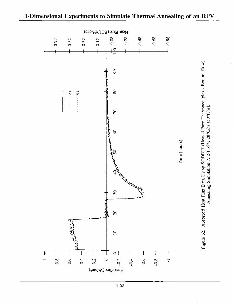
1-Dimensional Experiments to Simulate Thermal Annealing of an RPV
(09S- zy/nie) ™U n»H
f - i n <N
O o o O
0 0 o
oo 0 0 •3-
oo
3 O
E H
o
a o 4—* O
"Si 3 O CJ O ,
8 ^ - C o H o 4) o
IX, -a ID
S
8 s
O o 0 0 c
M.2 3 *3 CO • — I
:D 3 S
es <*> * • -tt, g •£ 3
g < <u
o 00
<
(N SO
=3 0 0
OO o
so o o o o o
SO O
oo o
G«»/AV) x n U * B 9 H
4-62

1-Dimensional Experiments to Simulate Thermal Annealing of an RPV 4.5 Test 4: 7°C/hr [12.5°F/hr]
4.5.1 Temperature Data
Temperature data for Test 4 are shown in Figures 63-79. Figure 63 shows heated face temperatures on the vertical centerline. Digital output shows the temperature control during the soak was better than ±0.7°C [±1.3°F] at 454°C [848°F] on F2 (top bank control TC), ±0.8°C [±1.4°F] at 454°C [848°F] on F13 (middle bank control TC) and ±1.0°C [±1.7°F] at 454°C [849°F] on F31 (bottom bank control TC).
Figures 64-72 show other temperature data on the heated and unheated faces. The temperature drop began at only about 4°C/hr [7°F/hr] but was increased to the correct value 7°C/hr [12.5°F/hr]. Results similar to Tests 2 and 7 can be seen on the heated face TCs (Figures 63-67) and unheated face TCs (Figures 70-72).
Figures 68 and 69 show temperature contour plots of the heated face of the RPV section at two times: the beginning (at about 63 hours) and end (at about 79 hours) of the soak. Good vertical temperature uniformity is evident in both figures. Both plots also show that the left side of the RPV section was cooler than the right side. At the beginning of the soak the average temperature and variation from the average of the RPV section was 454°C [850°F] ± 3%. At the end of the soak the average and maximum range was 453°C [847°F] ± 3%.
Figures 73 and 74 show temperature data from the concrete wall. Except for Wl, all TCs showed maximum concrete wall temperatures between 28°-33°C [82°-91°F]. Wl, the TC located highest on the concrete wall, was warmest, 42°C [108°F]. All TCs peaked before the cooldown began.
Figures 75-77 show through-wall temperature differences for the center vertical column (Figure 75), the center horizontal row (Figure 76), and the weld row (Figure 77). Temperature differences range from about 8°-19°C [14°-34°F] at the end of the rise portion at 63 hours to about 4°-15°C [7°-27°F] during the soak. Temperature differences at the end of the heat-up portion are smaller for this test than for either Test 2 or 7, due to a slower heat-up rate. However, during the soak, through-wall temperature differences are similar to those shown earlier.
Figures 78 and 79 show temperature differences on the heated and unheated faces, between TCs mounted on the weld locations and just below the weld location on the base metal. The temperature differences on the heated face range between +1°, -2.5°C [+1.8°, -4.5°F] and on the unheated face between 0° and +2°C [+3.6°F]. The shape of the curves in Figures 78 and 79 are similar to figures from earlier tests.
4-63
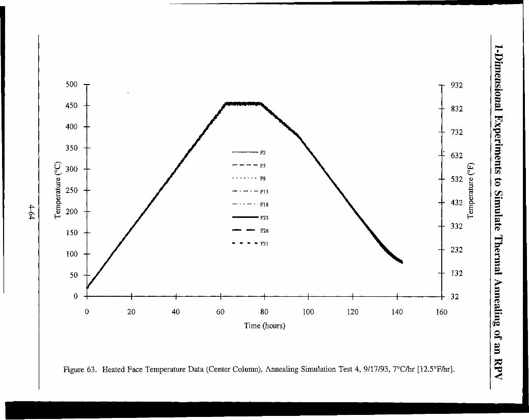
-r 932
- - 832
732
-- 632
532 g' 3
I H
0 20 40 60 80
Time (hours)
100 120 140 160
Figure 63. Heated Face Temperature Data (Center Column), Annealing Simulation Test 4, 9/17/93, 7°C/hr [12.5°F/hr].

20 40 60 80
Time (hours) 100 120 140
o
532 ^ c3
I H
160
Figure 64. Heated Face Temperature Data (Center Row), Annealing Simulation Test 4, 9/17/93, 7°C/hr [12.5°F/hr].
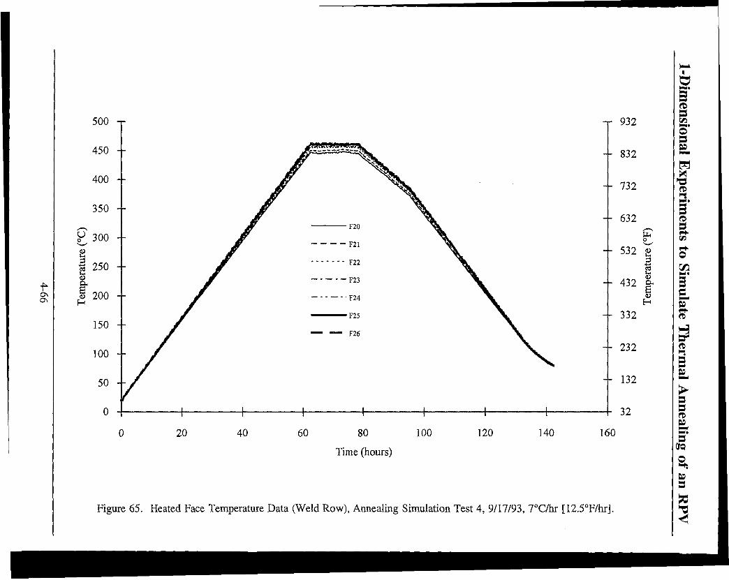
500 -r
20 40 60 80
Time (hours)
100 120 140 160
Figure 65. Heated Face Temperature Data (Weld Row), Annealing Simulation Test 4, 9/17/93, 7°C/hr [12.5°F/hr].
3 53
© S3 EL
B c , ST *-
H tyre
3 £L
= 9 CD SSL 3
oro s> is
»

-r 932
20 40 60 80
Time (hours)
100 120 140 160
Figure 66. Heated Face Temperature Data (Diagonal), Annealing Simulation Test 4, 9/17/93, 7°C/hr [12.5°F/hr],
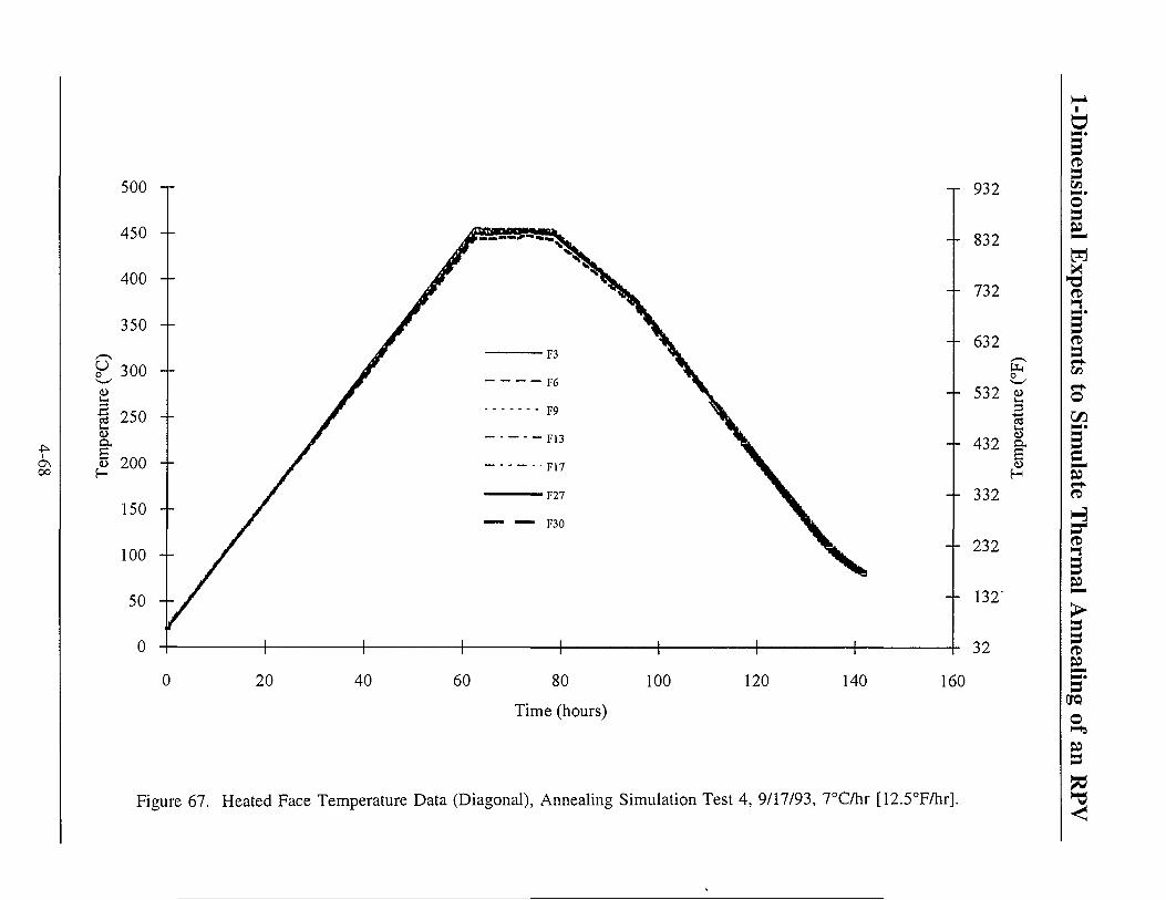
0 20 40 60 80
Time (hours)
100 120 140 160
Figure 67. Heated Face Temperature Data (Diagonal), Annealing Simulation Test 4, 9/17/93, 7°C/hr [12.5°F/hr].
CD
o S3 SL W CD
CD 3 «•*• t/3 <•+ O
ST i t -CD
H S3* CD > 1
B • S3 S3 CD
53 era o
S3
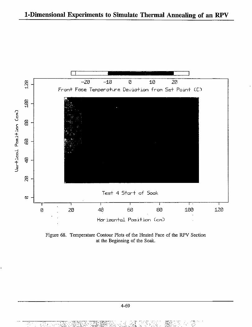
1-Dimensional Experiments to Simulate Thermal Annealing of an RPV
£ a \_i
c a + 19 a. H 0 a +
L Hi
z>
ca
(3
GJ f\l
<s -
-20 -10 0 10 20 Fron+ Face Tempera+ure Devia+ion from 5e+ Poin+ CO
Tes+ 4 5+ar-f of Soak i 0 20 40 60 80
Hdrison+al Posi+ion CcrO 100 120
Figure 68. Temperature Contour Plots of the Heated Face of the RPV Section at the Beginning of the Soak.
4-69

1-Dimensional Experiments to Simulate Thermal Annealing of an RPV
Itnt??
IN
H o ~ u
\ _ i Q r UJ n • H
~ t -
^ .S3
i i ~\ w -^ r
_j
H3 IN
a
n
-20 - 10 0 10 20 F ronr Face Tempera+ure Dev'-ia+ion f rom 5e+ Po in r tC" 1
l e s f 4 End of Soak
:0 40 60 80 Hor ason+al Posi+jLon l n""i
100 120
Figure 69. Temperature Contour Plots of the Heated Face of the RPV Section at the End of the Soak.
4-70

20 40 60 80
Time (hours)
100 120 140 160
Figure 70. Unheated Face Temperature Data (Center Column), Annealing Simulation Test 4, 9/17/93, 7°C/hr [12.5°F/hr].
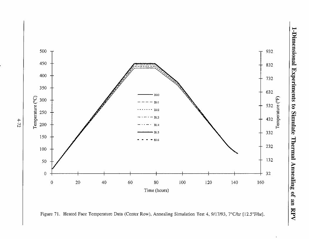
0 20 40 60 80
Time (hours)
100 120 140 160
Figure 71. Heated Face Temperature Data (Center Row), Annealing Simulation Test 4, 9/17/93, 7°C/hr [12.5°F/hr].

20 40 60 80 Time (hours)
100 120 140 160
Figure 72. Unheated Face Temperature Data (Weld Row), Annealing Simulation Test 4, 9/17/93, 7°C/hr [12.5°F/hr].

20 40 60 80
Time (hours)
100 120 140 160
CD S3
o EL
« • *
et-
O
I H tr B
& S3
CTQ
O
S3
Figure 73. Concrete Wall Temperature Data (Column), Annealing Simulation Test 4, 9/17/93, 7°C/hr [12.5°F/hr].

-J
20 40 60 80 Time (hours)
100 120 140 160
Figure 74. Concrete Wall Temperature Data (Row), Annealing Simulation Test 4, 9/17/93, 7°C/hr [12.5°F/hr].
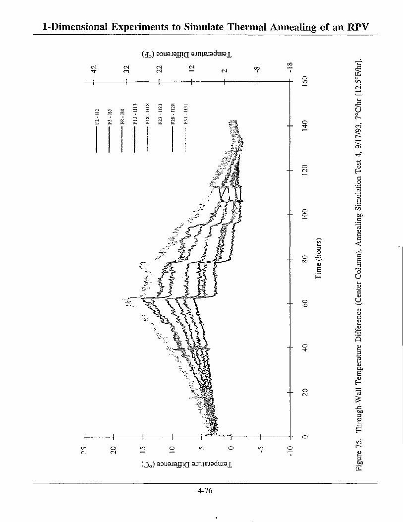
1-Dimensional Experiments to Simulate Thermal Annealing of an RPV
(do) 30U3J9JJIQ 9itl}eJ9dui3J[
C-l C-4
<N C-) oo
r-t <r\
o
o -3-
o
o o
o oo
0>
c
o o
o CI
o
( j 0 ) 90U9i9jgiQ gjnrejsdiuaj^
o
oi
u o
cn"
ON
<u H c .2 J3 S OO .s "3 C a <
B zi
~o U •_ <u
4—• G <D
U <u o c
<D a. 6 <u H
l
00 a o
IT)
3 DO
E
4-76

1-Dimensional Experiments to Simulate Thermal Annealing of an RPV
( j 0 ) 9DU9J9JJIQ 9JtUBJ9dU!9X
cs cs 00
I 00
o
o
o
O o
o oo
1 •I
o
o
o
(Do) 90U9J9J5IQ 9jnjBJ9dtU9X
o m
s en
•" • * - »
<D E-c o
1 a
CO
e
C
o
(U • 4 - *
c u lU o e <u
, u
P
£
00 3 o
X! E -
8 3 00
4-77
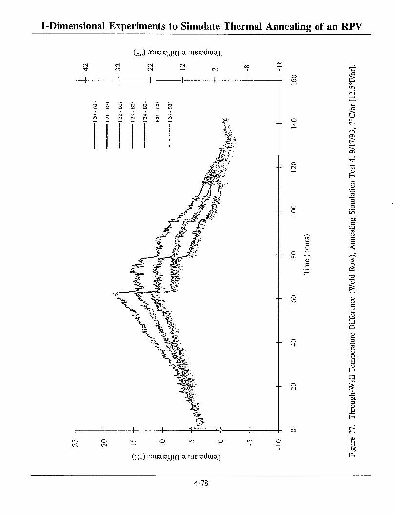
1-Dimensional Experiments to Simulate Thermal Annealing of an RPV
(>£0) 90U9J9JJIQ 9jraBJ9dUI9X
C I CN CN
CN CN 0 0
o — CN f-. -3- w-» \ D CM CS CN <N CN CN CN :2 — ™ £2 CZ C2 12
C N C N CN c s CN CN
•%a
• 4 ^ .ST
o
o
o CN
o o
GO I—
o CO ^
H
o
o
o CN
o
o
CN
=5 U o
r-en ON
as
CO 0)
H c o
00 CO)
c 13 C c < o
OS
<L>
O a <u
Q
C3 u. <D P .
a <u
E-13
i X ! 6 0
O u-,
X! H
o CN
(JQ) 99U9J9jgiQ 9JnjBi9dlU9J[^ 6 0
4-78

l-Dimensional Experiments to Simulate Thermal Annealing of an RPV
(j 0) souajajrtQ gjtuBjgdorax
as vo en en
t VO
I
o VO
O
O
o o
en i* 3 O
oo v - '
e
o VO
o "3-
o cs
en CS —i O <-f CS
( 3 Q ) 90U9J9JJIQ 9jnjBJ9dui9X
CO i n
o
cs*
«9 u
en
a\
en
£ o
s CO bo a
• *-« 1 3
<L> C5 C3
< 13
m i
^«3
<u c
a • 4 - *
2
<u H <D ca
i oo t-fi 3 bO
E
4-79
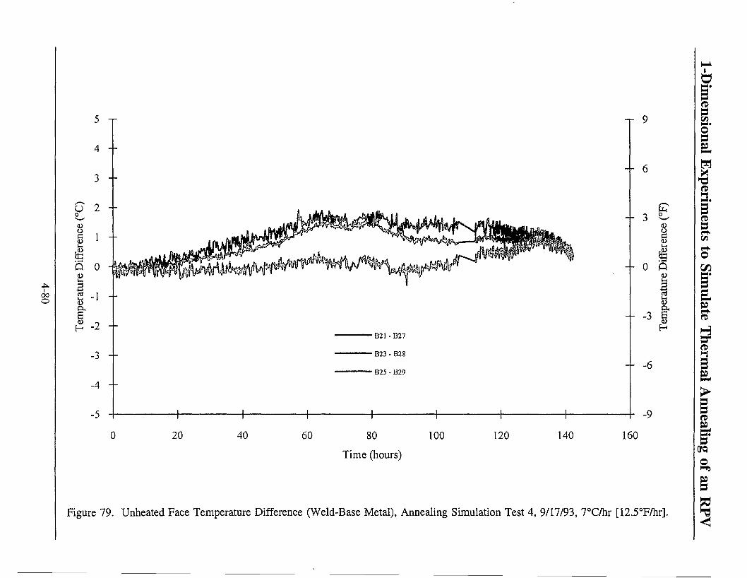
(J 0
o
2
c 1 <u 1
iffer
re
D
0
1 2 00 o
mpe
ra
-1
-2
1 0 Q
20 40 60 80
Time (hours) 100 120 140 160
9>
2
H
+ -6
-9
Figure 79. Unheated Face Temperature Difference (Weld-Base Metal), Annealing Simulation Test 4, 9/17/93, 7°C/hr [12.5°F/hr],
O
re
t/3
C/3
I to CD
H n B EL
re
I eta S,

1-Dimensional Experiments to Simulate Thermal Annealing of an RPV 4.5.2 Heat Flux Data
Figures 80-83 show heat flux data from Test 4.
Pyrheliometer Data - Incident Heat Flux
Pyrheliometer data are shown in Figure 80. As can be seen from the figure, HF3 reads higher than HF2. The reason for this difference is the same as described above in Section 4.3.2. The flux on the two gages rises from zero to about 0.11 W/cm2 [0.1 Btu/ft2-sec] just after zero time. Between 1 and 63 hours the gage outputs slowly rise, but HF2 rises less. HF3 reached the maximum value of about 2.11 W/cm2.[1.86 Btu/ft2-sec] and HF2 reached a maximum of 1.71 W/cm2 [1.51 Btu/ft2-sec]. HF3, during the soak between 63-79 hours, measured about 1.89 W/cm2 [1.67 Btu/ft2-sec]. HF2 shows a
9 9
heat flux of about 1.51 W/cm [1.33 Btu/ft -sec]. These values compare favorably with the predicted value of 1.59 W/cm2 [1.40 Btu/ft2-sec]. Similar to Test 2, the electrical input to the upper bank of heaters was greater than that to the middle bank; therefore, the output from the top pyrheliometer (HF3) should have been higher than that from the middle pyrheliometer (HF2).
The heat flux drops off in an exponential like manner at the beginning of the soak. Both gages show a sharp reduction in flux at 63 hours of about 0.22 W/cm2 [0.19 Btu/ft2-sec]. As will be seen below, the estimated absorbed flux from SODDIT just before the soak begins averages about 0.16 W/cm2 [0.14 Btu/ft2-sec], 27% less than 0.22 W/cm2 [0.19 Btu/ft2-sec].
SODDIT Data - Absorbed Heat Flux
Figures 81-83 show absorbed data generated from heated face TCs. All plots have the same basic shape with slightly different magnitudes. The absorbed heat flux values show more fluctuations or "noise" than on earlier tests. This could be due to the lower flux level and that any temperature fluctuation may have been magnified when SODDIT estimated heat flux. The absorbed heat flux rises sharply from zero to about 0.12 W/cm2 [0.11 Btu/ft2-sec] then rises more slowly up to about 0.16 W/cnT [0.14 Btu/ft2-sec]. The value of 0.11 W/cm2 [0.10 Btu/ft2-sec] compares favorably with the value given in Section 3.2 (0.12 W/cm2 [0.11 Btu/ft2-sec]). As soon as the soak begins, the absorbed flux drops sharply and eventually reaches zero. The absorbed flux continues at zero until the cooldown portion begins, when the absorbed flux goes sharply negative. As the temperature of the RPV section slowly drops to ambient, the absorbed flux rises due to a decreasing rate of heat loss. These characteristics are the same as those in earlier tests.
4.6 Air Flow Data
The air flow used to simulate reactor cavity cooling was based on a Westinghouse 2-loop design. The specifications were described in Section 3.3; the minimum flow velocity was 203 m/min [666 ft/min @ 4650 CFM]. Initially, a rectangular shaped, horizontally mounted duct was used to distribute the air upward between the concrete wall and the back side of the mirror insulation. Uniformity was poor with the rectangular duct so a circular duct (also horizontally mounted) with flow diverters was fabricated. This arrangement resulted in much better air flow uniformity (see Figure 8).
4-81

2.5 -r
20 40 60 80
Time (hours)
100 120 140
- - 2
1.5
S X 3
0.5
160
Figure 80. Incident Heat Flux Data (Pyrheliometers), Annealing Simulation Test 4, 9/17/93, 7°C/hr [12.5°F/hr].
o S3
< • * -
O
3 ST
H sr TO
3 EL >
ft £L 5'
era o so 3 ^3

0.2 -r -r 0.18
0 0
-0.2 -1- -0.18
Time (hours)
Figure 81. Absorbed Heat Flux Data Using SODDIT (Heated Face Thermocouples), Annealing Simulation Test 4, 9/17/93, 7°C/hr [12.5°F/hr].

1-Dimensional Experiments to Simolate Thermal Annealing of an RPV
(S-zWfllS) Xtlfcl JB3H 00 1 — <
CN O
o o O
VO
o ©
0 0
o I
3 o CD
£
£ o Pi u, (U
4—»
a a) U 00 <0 U , 3 O c> j |
rmo -5 rmo
UH o; o
-G >/> H (N D O a Ut
U-. •5s
X I U a; o
4—. r--(i) ** a ON
F- r-i—i p ON
p o "fr CO 00
<1>
c H 00
tion
rt rt ul
a
P c X CO 3 bi)
UH c 4—* CTf a 11) <D X G
G X j < OJ
- O 1-. O O0
X) < <N OO <U 1-1 3 W)
UH
O i—I
o VN
o o o
(JUJO/SUBAV) xnj j JB9H
4-84

1-Dimensional Experiments to Simulate Thermal Annealing of an RPV
(s-twnxa)xnH^H 00 1—1 r—1 o o o o
o OJ 00
o o o
o - - o
__ o
O
o en
O CM
o
3 O
a
o
CN
6 y - » • -
o
s o
• * - >
o i
"el a o o o a l-l <L>
X 5 H PL,
<D •4—*
d
K ON
H £ Q <* 8 * O ~ M H
• ^ 2
•a 3
Q.S x w
a bo E .S
1—H
ffi a 4) l-l O
< cn oo a 00
HH
o in o
>n o
IT)
o o"
(ZUIO/SWBM) xnjg jean
4-85

1-Dimensional Experiments to Simulate Thermal Annealing of an RPV The flow rate was constant for all the tests. Air flow measurements were taken between Tests 2
and 3 and after Test 4 to ensure that no significant changes in the air flow rates occurred due to equipment malfunction. In addition, a series of five additional checks were made to obtain a reasonable number of values for each location. All measurements were made with an Alnor Velometer, Jr., Type 8100. This handheld device had two velocity ranges, 0-150 m/min [0-500 ft/min] and 0-760 m/min [0-2500 ft/min] scales. Because the measured air velocity varied between 150-275 m/min [500-900 ft/min], the high range had to be used, so less resolution was available than if the low range were used.
Measurements at five locations were taken at the top of the cavity between the back of the mirror insulation and the concrete wall. Table 5 shows a summary of the data, showing averages of the velocity at each of the five locations from all seven sets of data. Figure 84 shows a sketch describing where the measurements were taken. See Section 4.8 for a short discussion of air flow measurement errors.
Table 5: Air Flow Velocity Measurements Location Air Velocity, m/min [ft/min] Comments
1 168 m/min [550 ft/min] Closest to fan, gap 10 cm [4 in]
2 223 m/min [732 ft/min] Second highest velocity
3 218 m/min [714 ft/min] Center of cavity, gap 5 cm [2 in]
4 248 m/min [814 ft/min] Highest velocity
5 179 m/min [586 ft/min] Farthest from fan, gap 10 cm [5 cm]
Using all 5 locations, the average air velocity through the cavity was about 207 m/min [680 ft/min], which is within the minimum air velocity specification given in Section 3.3. Because this air velocity was close to the minimum, the measured concrete temperatures would be the highest expected, and therefore, would represent conservative (upper) limits. As a result, one could say that the maximum expected concrete temperature would be about 44°C [111°F]. One might expect that, because the air flow was lowest at locations 1 and 5, thermocouples W6 and W9 would read the highest temperature. This is the case on Test 2, Figure 28, but not on Tests 3 and 4, Figures 53(b) and 74. However, differences between the highest and lowest TCs are only about 5°C [9°F] and may not be significant.
4.7 Power Input to Heaters
Power input to all 3 heater banks was recorded for each test. Power input to the heater banks versus time for the tests are shown in Figures 85-88. There are several trends evident in the data. The power to the bottom bank of heaters was substantially higher than to either the middle or top bank. This was due to the large heat sink facing the bottom bank of heaters: the steel supporting frame.
The middle bank of heaters consistently consumed less power than either the top or bottom bank. This was due to a coupling effect: part of the energy emanating from the bottom heater bank was transmitted to the middle of the RPV section and similarly from the top heater bank. Note that the reverse is also true.
4-86
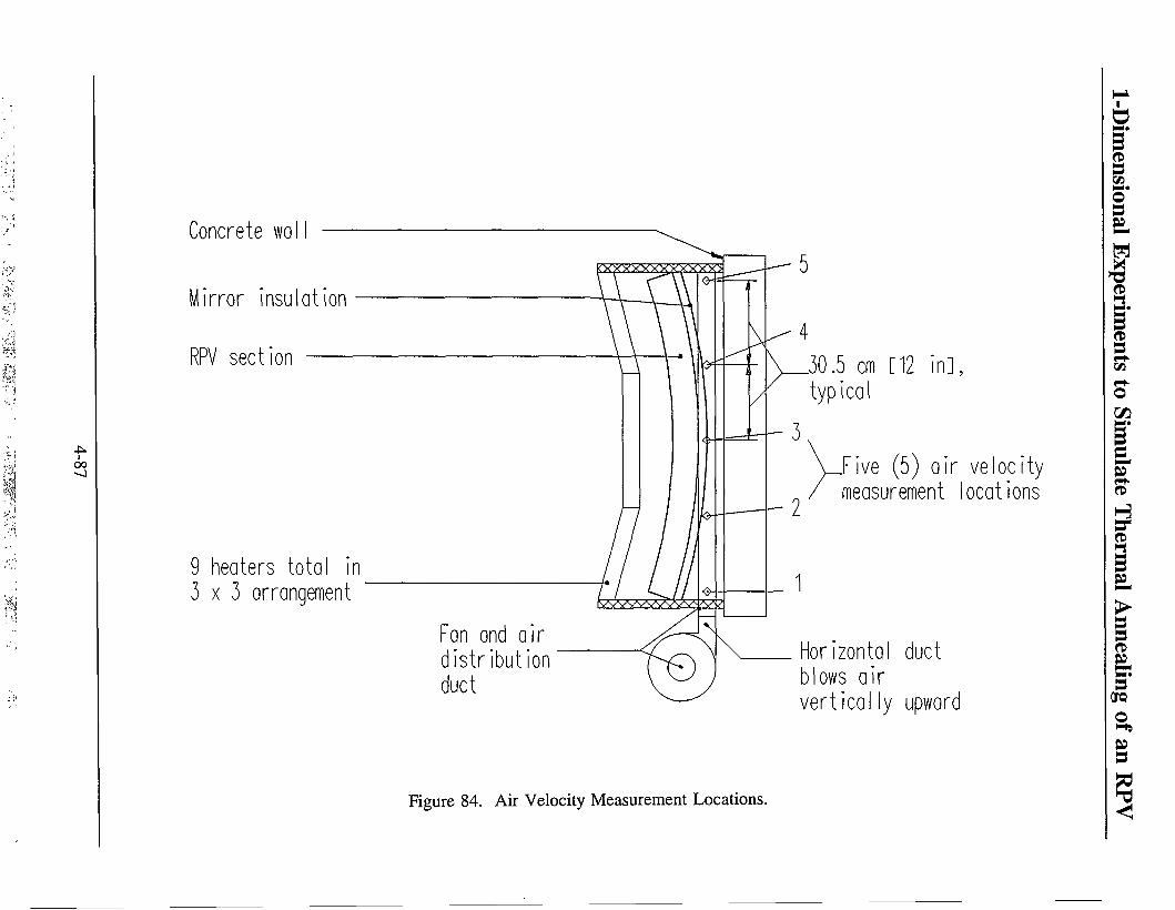
Concrete wal
Mirror insulation
RPV section
oo
9 heaters total in 3x3 arrangement
Fan and air distribution duct
.30.5 cm [12 in] , typical
f i ve (5) air velocity measurement locations
Horizontal duct blows air vertical ly upward
Figure 84. Air Velocity Measurement Locations.
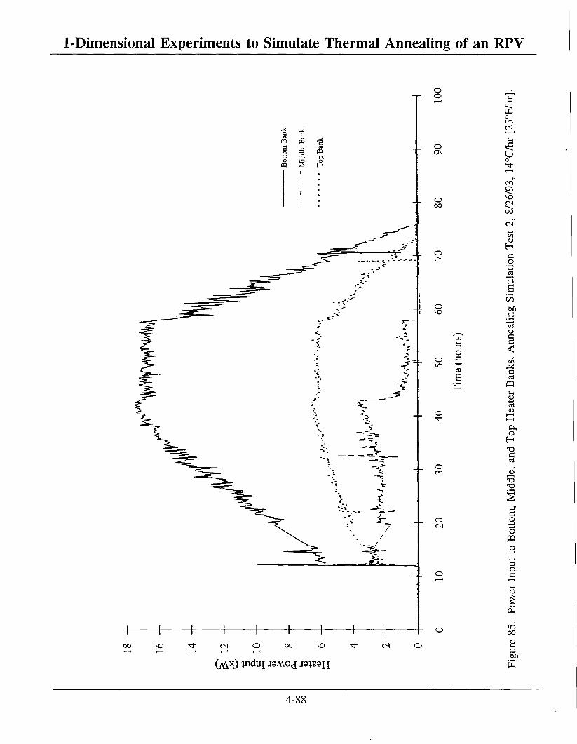
1-Dimensional Experiments to Simulate Thermal Annealing of an RPV
M
I 85
^ •u £
T3 m •o D.
s £
o (N
U
CT\
Co (N oo
<u E - " c .2
• * — »
c3
00 00 c • ^H
ctf <L)
CO C U, C 3 O <
J3 tr\ CO
M a a
<D
a, o H X) a
X ) T3
O PQ o
3 a, c
o 0-, in oo
oo vo (N VO <N
(AV5!) J n d u I J3AV0J J9JB3H 3 GO
4-88

1-Dimensional Experiments to Simulate Thermal Annealing of an RPV
I
oo MD cs o oo ^o ^r
(AVH) jnduj J9M.0(i J3JB9H
(N
S o O vn
u o
oo
en ON
<D
H c o
6 oo GO c
• »-( 1 3 <u c c
<
c «j
PQ
u .
<D
o H
C
T3
o « o 3 & e
o
oo
3 60
4-89
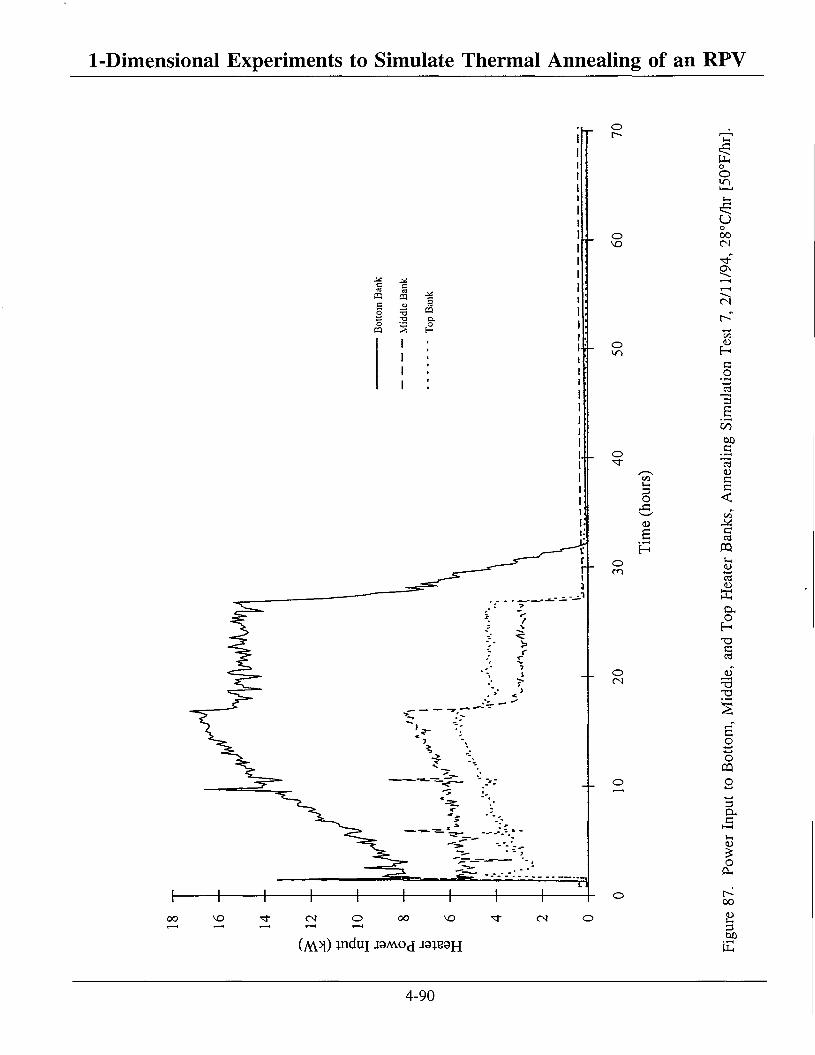
1-Dimensional Experiments to Simulate Thermal Annealing of an RPV
03 en ^i
UIO die SB
£2 -o o.
o
o r-
o
o
3 O
•C CD
s o CO
o (N
VO (N VO <N
(AV>D jndui JSAVOJ J9JB9H
o o
u o oo n • < *
ON
CM
r-" 1/3 <u
H c o
• > — t • * — »
cj —H
s CO 00 c 13 t> c c < t/T
Jxi C «J
PQ s-l <u
•i—t
a, o H 13 C
jo T3 -a
c o O
3 a
O OH
oo
3
E
4-90

18 -r
16
14
£ 12 £ • M
3
Inp 10
u, 0)
£ o tf PH u c> •t-i OS
HI 6
4 t'uM v . .__.
Bottom Bank
Middle Bank
Top Bank
»-fj:..r.—a-nr^lmKiM i f i i
20 40 60 80
Time (hours)
100 120 140 160
Figure 88. Power Input to Bottom, Middle, and Top Heater Banks, Annealing Simulation Test 4, 9/17/93, 7°C/hr [12.5°F/hr].
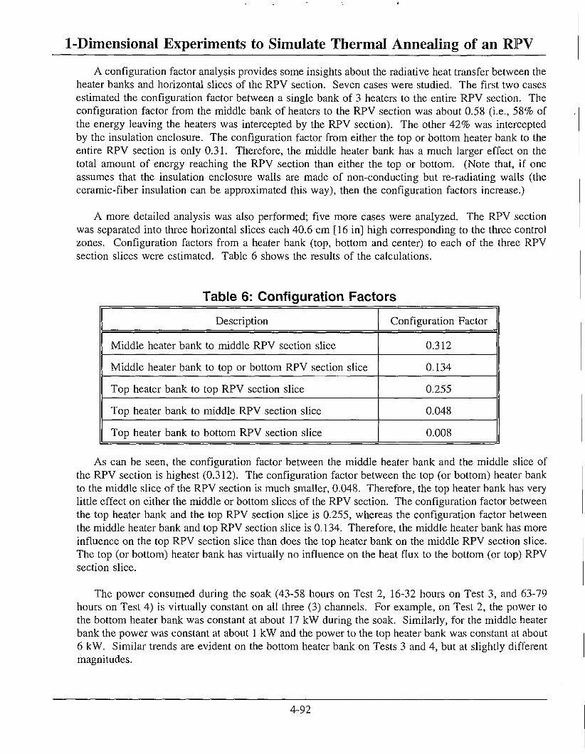
1-DimensionaI Experiments to Simulate Thermal Annealing of an RPV A configuration factor analysis provides some insights about the radiative heat transfer between the
heater banks and horizontal slices of the RPV section. Seven cases were studied. The first two cases estimated the configuration factor between a single bank of 3 heaters to the entire RPV section. The configuration factor from the middle bank of heaters to the RPV section was about 0.58 (i.e., 58% of the energy leaving the heaters was intercepted by the RPV section). The other 42% was intercepted by the insulation enclosure. The configuration factor from either the top or bottom heater bank to the entire RPV section is only 0.31. Therefore, the middle heater bank has a much larger effect on the total amount of energy reaching the RPV section than either the top or bottom. (Note that, if one assumes that the insulation enclosure walls are made of non-conducting but re-radiating walls (the ceramic-fiber insulation can be approximated this way), then the configuration factors increase.)
A more detailed analysis was also performed; five more cases were analyzed. The RPV section was separated into three horizontal slices each 40.6 cm [16 in] high corresponding to the three control zones. Configuration factors from a heater bank (top, bottom and center) to each of the three RPV section slices were estimated. Table 6 shows the results of the calculations.
Table 6: Configuration Factors Description Configuration Factor
Middle heater bank to middle RPV section slice 0.312
Middle heater bank to top or bottom RPV section slice 0.134
Top heater bank to top RPV section slice 0.255
Top heater bank to middle RPV section slice 0.048
Top heater bank to bottom RPV section slice 0.008
As can be seen, the configuration factor between the middle heater bank and the middle slice of the RPV section is highest (0.312). The configuration factor between the top (or bottom) heater bank to the middle slice of the RPV section is much smaller, 0.048. Therefore, the top heater bank has very little effect on either the middle or bottom slices of the RPV section. The configuration factor between the top heater bank and the top RPV section slice is 0.255, whereas the configuration factor between the middle heater bank and top RPV section slice is 0.134. Therefore, the middle heater bank has more influence on the top RPV section slice than does the top heater bank on the middle RPV section slice. The top (or bottom) heater bank has virtually no influence on the heat flux to the bottom (or top) RPV section slice.
The power consumed during the soak (43-58 hours on Test 2, 16-32 hours on Test 3, and 63-79 hours on Test 4) is virtually constant on all three (3) channels. For example, on Test 2, the power to the bottom heater bank was constant at about 17 kW during the soak. Similarly, for the middle heater bank the power was constant at about 1 kW and the power to the top heater bank was constant at about 6 kW. Similar trends are evident on the bottom heater bank on Tests 3 and 4, but at slightly different magnitudes.
4-92

1-Dimensional Experiments to Simulate Thermal Annealing of an RPV However, on Test 7 (Figure 87) a different behavior occurred. During the heat-up portion, the
middle bank consumed noticeably more power than the top bank, unlike Test 3 (Figure 86). As soon as the soak began, the power to the middle bank dropped below the top bank, but only to about 2.5 kW. The bottom bank consumed about 15 kW and the top about 4 kW during the soak. These are different than on Test 3, at the same heat-up rate. It is apparent that there is more than one way to effect a uniform temperature on the heated face using multiple heater banks.
During the initial rise portion, the power consumed during Test 2 at 14°C/hr [25°F/hr] heat-up rate was less than that consumed during Test 3 at 28°C/hr [50°F/hr] heat-up rate, and the power consumed on Test 4 at 7°C/hr [12.5°F/hr] heat-up rate was less than either of the first two tests. This would be expected because the power input required to effect a 28°C/hr [50°F/hr] heat-urjjrate should be higher than that required to effect a 14°C/hr [25°F/hr] heat-up rate and similarly for the slowest heat-up rate (7°C/hr [12.5°F/hr]).
4.8 2-Dimensional Effects
Although these tests were designed to be 1-dimensional, due to temperature non-uniformity on the heated face 2-dimensional heat transfer occurred. To obtain estimates of the magnitude of the 2-dimensional heat transfer, temperatures at 30 hours were analyzed. The lateral heat conduction (horizontal and vertical heat conduction on the heated face) was estimated by using temperatures on the heated face, distances between TCs and the thermal conductivity:
lateral = kAT/Ax, [8]
where q is the lateral heat conduction (horizontal or vertical direction), AT is the temperature difference between heated face TCs and Ax is the distance between the TCs. Using this method, lateral heat conduction estimates were made for the heated and unheated faces at 30 hours on Test 2. Results show that, assuming a nominal absorbed through-wall heat flux of 0.29 W/cm [0.26Btu/ft -sec] and correcting for the different area elements involved (i.e., A l a t e r a l / A f a c e = 0.5625), the average 2-dimensional, lateral heat transfer was about 9% of the nominal value in all vertical and horizontal locations except the top row (TCs Fl, F2 and F3). In the top row, the 2-dimensional heat transfer was much greater, about 29% of the nominal value, due to the large temperature gradient seen on the contour plots, Figures 22 and 23.
An alternate method of estimating 2-dimensional, lateral heat transfer uses a total energy balance on a through-wall area element of the RPV:
Qtess- A f a c e + 4 ^lateral x Alateral + <3rf A face + ^e A face = fair + ^c) Aface &] fc**CK
Personal communication from Walt Gill, Energetic and Environmental Test Department 2761, to Jim Nakos, Advanced Nuclear Power Technology Department 6471, September 2, 1994.
4-93

1-Dimensional Experiments to Simulate Thermal Annealing of an RPV or, dividing by A f a c e :
lateral w nm 44**- + ~ A
X ^lateral + 4rf + 4e = 4ir + ?c [ 1 0 ]
boxK. Aface
where q r f, q e, q i r, and q c were defined in Section 4.3.2, q ack is the heat loss from the unheated side and 4(A l a t e r a l /A f a c e ) is the ratio of the area of the RPV perimeter divided by the area of a face.
Using estimates from Test 2 from pyrheliometers HF1, HF3, and HF2, the 2-dimensional, lateral heat transfer was about 18% of the nominal value [0.29 W/cm2 [0.26 Btu/ft2-sec]. Although twice the value estimated using the first method [9%], it is of the same order of magnitude. Due to the difficulties in accurately estimating all of the terms in equation [10], it is likely the least accurate estimate.
As a result of the 2-dimensional estimates, one should not use heat flux estimates from SODDIT from top row TCs (Fl, F2, or F3), or as explained below, from the bottom row TCs (F30, F31, or F32). Due to the significant 2-dimensional horizontal heat transfer on the top row, a significant portion of the heat transfer measured by top row TCs was due to 2-dimensional lateral heat conduction, not through-wall (1-dimensional) heat conduction. The effect of the 2-dimensional heat conduction is to cause a decrease in power required. Because part of the energy affecting the TC is due to lateral, 2-dimensional heat conduction, a lesser amount is through-wall heat conduction. As a result, the through-wall temperature difference is greater for top row TCs. This behavior can be seen in Figure 29. Also from Figure 29, the temperature difference between the bottom row TCs F31-B31 is large as compared with others. This also implies a larger 2-dimensional effect near the bottom than near the middle.
Even though virtually all of the absorbed heat flux plots for each test read the same, the user should concentrate on the center row (F10-F16) for heat flux data. Temperature differences in the center row are much smaller than those on either the top or bottom (Figure 29). Therefore, for the best 1-dimensional data, one should concentrate on the center row measurements.
4.9 Measurement Errors/Uncertainties
4.9.1 Thermocouple Mounting Errors
As stated in Section 3.4, stainless steel (SS) sheathed (sheathed to the tip), ungrounded junction thermocouples (TCs) were selected over glass sheathed TCs for use during the experiments. Intrinsic TCs are the preferred method of mounting, the one with the lesser error, because each of the wires is in intimate contact with the surface (see Figure 89). However, experience at Sandia National Laboratories' Radiant Heat Facility using sheathed TCs with the tip of the sheath stripped away (intrinsic/exposed junction) has been, in general, that TCs are not very reliable, and in some instances will give reasonable, but erroneous readings . Grounded junction TCs provide slightly better temperature indication than an ungrounded junction TCs because they are in better contact with the
Sandia National Laboratories Internal Memorandum RS7531/82/1, "A comparison of Exposed Junction, Grounded Junction, and Ungrounded Junction Thermocouples," by J.T. Nakos and J. Gabaldon, July 20, 1982.
4-94
1-Dimensional Experiments to Simulate Thermal Annealing of an RPV surface one is trying to measure. However, the improvement over ungrounded junction sheathed TCs is marginal and DAS failures can compromise grounded TC measurements because all TCs are electrically connected through the metal surface. Therefore, as stated in Section 3.4, in the interest of obtaining the most reliable data, fully sheathed, ungrounded junction TCs were used.
In addition to Tests 2, 3,4, and 7 described above, two additional tests were performed to measure the difference in temperature response between ungrounded junction sheathed TCs and five (5) additional exposed junction (intrinsic) TCs (Tests 5 and 6). Except for the exposed junction at the tip, where the sheath was stripped away, the TCs were of the same type. The intrinsic TCs were mounted directly (welded) adjacent to corresponding sheathed TCs. Therefore, temperature differences seen between the two types of TCs would be due only to the method of mounting the measuring junction.
Figures 90 and 91 show results of the tests (Tests 5 and 6). Figure 90 (Test 5) shows results from a 7°C/hr [12.5°F/hr] heat-up rate and Figure 91 (Test 6) shows results from a 14°C/hr [25°F/hr] heat-up rate.
Throughout the time shown in Figure 90, the temperature was rising at 7°C/hr [12.5°F/hr]. F10-INT10 is the difference between TC F10 (on the front surface) and the intrinsic TC mounted adjacent to F10. Similar results are plotted for F11-INT11, F12-INT12, F13-TNT13, and F14-INT14. During the early part of the test, the intrinsic TC reads slightly higher than the sheathed TC, causing the difference to be negative. This could have been due to initial conditions (i.e., the RPV section was slightly warmer than the surrounding air). As a result, the sheathed TC read slightly less than the intrinsic TC. However, at about 12 hours the differences begin rising and after about 26 hours all of the sheathed TCs consistently read higher than the intrinsic TCs, causing the difference to be positive. The maximum differences at the top of the rise (62 hours) range from about 2.2°-5.0°C [4°-9°F]. (Note the DAS hardware problems between 41-55 hours.)
4-95
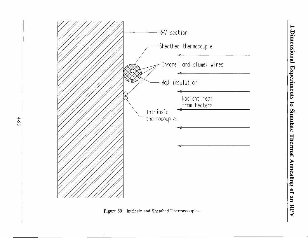
RPV section Sheathed thermocouple
-s3-
Chromel and alumel wires • o
MgO insulation -&-
Radiant heat from heaters
nsic thermocouple
-«a-
•<3r
•<a-
Figure 89. Intrinsic and Sheathed Thermocouples.
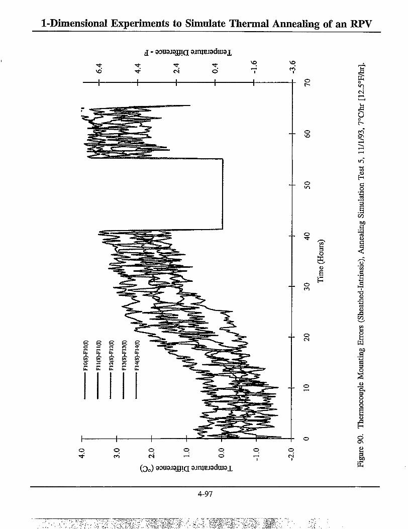
1-Dimensional Experiments to Simulate Thermal Annealing of an RPV
g - aousjagia aimuradurai ^4-
© vq
• \q
3 O
b b b b b A A A A C/> CO 00 CO CO o cs CO •fl-b b b b b
o o tri <N
o
(Q 0 ) souajagra ainmradurax
o
e-i
s o
CO
<u H a o
J? a
CO
a
a 5 o
°3 a
s •
X I <u -3 ca <D
CO
o a w a
•*3 G 3 O
JO "el 3 O o o
H
o s 3
4-97

1-Dimensional Experiments to Simulate Thermal Annealing of an RPV
(io) swdisjgfj 9jruBi3durax
7.0
2.0
-3.0
-8.0
-13.
0
-18.
0
i i i i i o I 1 1 I I oo
§ e § r l T
fc. U H b tt. l i .
A, ,A^. ^ , i v - J ~ C> CO CO
o r } •v u. U , t , [ 1 . u.
o
o
o
o 3 O
Si 0) E H
o
O
o o r4
o o
o o •St-
o o od
o o
(Do) sousJSJffiQ sJiUBjaduiax
PL, o
o •si-
CO
oo
CO <u
H a .2
B 00 c 73 <u c c <
CO c
•3 <D
CO
o w a a 3 O
"E< 3 O o o <u
E -
3 00
4-98

1-Dimensional Experiments to Simulate Thermal Annealing of an RPV Figure 91 shows results from Test 6. (Again, there was a problem with the DAS from about 10-23
hours, and because this was during non-working hours, the problem was not discovered until the next day.) Although data acquisition ceased, the heaters continued on track. From about 0-27 hours, the RPV temperature rose at 14°C/hr [25°F/hr], from 27-38 hours the temperature was held constant, and from 38-50 hours the RPV temperature dropped. Figure 91 shows temperature differences between the sheathed and intrinsic TCs (F10-INT10, F11-INT11, F12-INT12, F13-INT13, and F14-INT14). During the early part of the test, intrinsic TCs read slightly higher than the sheathed TC, causing the difference to be negative, similar to Test 5. However, between 0-5 hours the differences begin rising and the sheathed TCs consistently read higher than the intrinsic TCs, causing the difference to be positive. The maximum differences range from about 2.0°-4.0°C [3.6°-7.2°F].
One explanation for the positive differences is that, because the sheath and magnesium oxide insulation are "protecting" the chromel and alumel wires, the measuring junction is being insulated from the surface as compared to the intrinsically mounted TC. The incident heat flux is directed towards the RPV surface and on the sheathed TC. Because contact between the sheathed TC and the surface is not as good as compared with the intrinsic TC, the temperature of the sheathed TC should read slightly higher than that of the RPV section. Because the intrinsically mounted TC wires are welded directly onto the surface, it would read closer to the RPV section surface, which is lower than that measured by the sheathed TC. Similar results were described in the Internal Memorandum in footnote 5, where simulated fire temperatures (1010°C [1850°F]) were being measured. At these high temperatures, differences between ungrounded junction sheathed TCs and exposed junction, intrinsically mounted TCs were up to 8% 82°C [150°F]. This is considerably more error than that seen in Figures 90 and 91, but the trend is similar.
In summary, the temperatures presented in this report may be about 5°C [9°F] above the actual RPV temperature due to the "mounting method." This is about a +1.1% error.
4.9.2 Thermocouple Uncertainties
As discussed earlier, the uncertainty of standard precision TCs from the factory is ±3/4% between 293°-1256°C [559°-2282°F]. Reference [10] presents a detailed discussion of thermocouple measurements at the Radiant Heat Facility. Uncertainties in the data acquisition system used at that time ranged from ±2.9% at low temperatures (179°C [354°F]) to ±1.5% at high temperatures (1200°C [2192°F]). Linearly interpolating between the two temperatures gives ±2.5% uncertainty at 454°C [850°F]. Uncertainties are due to several sources: DAS hardware, TC reference junction, thermocouple extension wire, and the voltage to temperature conversion equation. The voltage to temperature equation is a polynomial that approximates experimental data, and therefore has some uncertainty in the conversion. The two temperature ranges are due to the 4 order polynomial used to convert the voltage output to temperature (same conversion equation is still being used). Different polynomials are used in different temperature ranges (one temperature range ends at 179°C [354°F]). The ±2.9% and ±1.5% values do not include uncertainties due to the TC mounting scheme used (e.g., ungrounded junction sheathed, exposed junction) and electrical noise generated in the DAS output. At 10-20 kW power levels (similar to those in the tests described herein), up to several hundred uV noise was induced into the DAS output. This converts to about ±1.5°C [±2.7°F] or about ±0.3%. Summing the sources of uncertainty in the TC measurements at the hold temperature (454°C [850°F]), one gets:
Total uncertainty in TC measurements = ±2.5% ±0.3% ±0.75% = ±3.6%.
4-99

1-Dimensional Experiments to Simulate Thermal Annealing of an RPV Using the "SRSS" method (square root of sum of squares, accepted by the Instrument Society of America (ISA)), one gets:
Total uncertainty in TC measurements = (2.5 2 + 0.3 2 + 0.75 2) 1 7 2 = ±2.6%.
In actuality, when the system was calibrated, the uncertainties were less than either ±3.6% or ±2.6%. When an NBS traceable calibrator was used to check the entire system, excluding the TCs, the system consistently read to within ±1% or better up to 524°C [1000°F].
4.9.3 Thermocouple Measurement Error Implications
The implications of measurement errors on an actual anneal could be significant. During an actual anneal, TCs used to measure RPV temperatures may be mounted as in the Russian design, as part of the heating apparatus lowered into the RPV. In that design (see [5] in Section 6) "retractable" TCs were used to measure the RPV inside wall temperature. TCs were encased in the end of a spherical ball about 1.3 cm [0.5 in] diameter and pressed against the RPV wall using a retractable weight and level arrangement. There was no discussion regarding TCs errors associated with this measurement scheme, but a subsequent discussion with an author of the report brought out that mounting method errors of 6°-8°C [11°-14°F] were measured . Determination of mounting method measurement errors incurred using retractable TCs or other methods would be very beneficial to allay regulatory concerns.
4.9.4 Pyrheliometers - Incident Heat Flux Uncertainties
Uncertainties in pyrheliometer outputs were listed in Section 3.4 as +3%, -6%. These are gage uncertainties. Accuracy of the gage calibrations and the uncertainties in the measurement of the gage output also needs to be approximated. Calibration sheets provided from the manufacturer (HY-CAL Engineering) are hard copy sheets of heat flux versus output voltage. No curve fit is provided. The calibrations from the manufacturer for all three (3) pyrheliometers were linear to within ±3%. Heat flux measurements do not incur the same uncertainties that TC measurements do. For example, uncertainties due to TCs, TC extension wire, voltage to temperature conversion, and TC reference junction do not apply to pyrheliometer heat flux measurements. Of the ±2.5% uncertainty used for TC measurements, only the uncertainty associated with DAS (e.g., electronics) remains. At the 10 mv output of the gages, the error is about ±0.33% [10]. Therefore, the total uncertainty in pyrheliometer heat flux measurements is:
Total uncertainty in pyrheliometer heat flux measurements = +3%/-6%, ±3%, ±0.3% = +6.3%, -9.3%.
Personal conversation between Noman Cole, MPR Associates, Inc., and Jim Nakos, Sandia National Laboratories, February 18, 1994.
4-100

1-Dimensional Experiments to Simulate Thermal Annealing of an RPV 4.9.5 Estimated Absorbed Heat Flux Uncertainties from SODDIT
There are several sources of uncertainty in absorbed heat flux measurements generated by SODDIT. The most important sources are the following:
• Uncertainties due to inaccurate material properties • Uncertainties due to inaccurate temperature measurements • Uncertainties due to 2-dimensional heat transfer effects on the 1-dimensional SODDIT
calculations. Each of these uncertainty sources are discussed below.
Uncertainties due to inaccurate material properties are difficult to estimate. The most accurate material properties available in the literature (e.g., thermal conductivity, specific heat) for stainless steel (cladding) and A533B steel (base metal) were used as input to SODDIT [11], [12], [13]. It was not possible to destructively sample the RPV section (and would have been prohibitively expensive) to measure the exact material properties for the RPV section tested. As a result, uncertainties due to inaccurate material properties cannot be quantitatively estimated. However, because thermal properties do not change significantly within steel grades, it is expected that uncertainties due to inaccurate material properties are relatively small compared to uncertainties from other sources.
A sensitivity analysis using noisy temperature data was performed to assess the errors on inverse heat conduction calculations.9 The temperature input into SODDIT was created by generating a closed-form solution temperature history for an insulated flat plate response to a triangular heat flux. Noise was added to the temperature input by introducing a normally distributed random noise level to the signal. It was found that a temperature signal with a error of 1.1 °C [2°F] (standard deviation) caused an 11% error in the estimated heat flux for "low" (less than 260°C [500°F]) temperatures. For higher (greater than 260°C [500°F]) temperatures, the error for the same temperature error (1.1°C [2°F] standard deviation) rose to 29%. Lower heat flux errors were found for lower temperature input errors. The reason for the error increase at higher temperatures was due to increasing values of thermal diffusivity (k/cp). Increasing values of thermal diffusivity causes increased stability in SODDIT calculations, whereas decreasing values causes larger instabilities and therefore larger errors.
In the 1-dimensional tests, the thermal diffusivity of both the stainless steel cladding and A533B base metal decreased with temperature. Therefore, one might expect larger instabilities in the absorbed heat flux data as the temperature of the RPV section rose. Upon viewing the heat flux graphs presented earlier, there is not a consistent pattern of increased noise or oscillations as time progresses. However, it does seem that some TCs are much noisier than others throughout the test.
Uncertainties due to inaccurate temperature measurements were quantitatively measured using data from Test 2. The output from several TCs (Fl, F2, and F13) were approximated using a linear curve during the heat-up portion of the test. This part of the test was chosen because the heat flux was nonzero, whereas during the soak the absorbed flux dropped to zero. The linear "fit" provided the equation that approximated the data and an estimate of the "standard error" (uncertainty), which is the same as
"Sensitivity Analysis for Noisy Temperature Data in Inverse Heat Conduction Calculations," J.J. Gregory, 6414 to N.R. Keltner, 7537, April 2, 1987.
4-101
wmmTm^mmM::^:- . ->>mm^m;m--i:
1-Dimensional Experiments to Simulate Thermal Annealing of an RPV the SRSS method discussed in Section 4.9.2. (The analysis was performed on the spreadsheet program "Quatro Pro for Windows, Version 1.") The TC data was very accurately modelled using a linear curve, as expected because the control system was programmed to follow a linear temperature heat-up rate of 14°C/hr (actually 13.89°C/hr) [25°F/hr]. TCs F2 and F13 were used as control TCs, and the slope of the linear approximations were estimated to be 13.91°C/hr [25.04°F/hr] and 13.90°C/hr [25.02°F/hr], respectively. Standard errors (temperature uncertainties) for the three TCs (Fl, F2, and F13) were 0.63°C [1.13°F], 0.51°C [0.92°F], and 0.41°C [0.74°F], respectively. As can be seen, temperature control during the heat-up portion of the test was very close to the desired rate of 13.89°C/hr [25°F/hr] with an average uncertainty of 0.52°C [0.93°F].
Absorbed heat flux values for these TCs were also generated (several are discussed in Section 4.3). A linear fit was also used to approximate the heat flux data; as can be seen from the absorbed heat flux plots shown in Figures 35-37, the heat flux rise from 24-40 hours appear almost linear. For the same three TCs, absorbed heat flux uncertainties from linear approximations were 0.0075 W/cm2 [0.0066 Btu/ft2-sec] for Fl, 0.0083 W/cm2 [0.0073 Btu/ft2-sec] for F2, and 0.0074 W/cm2 [0.0065 Btu/ft2-sec] for F13. The nominal temperature at 30 hours on TC F13 was about 273.7°C [524.6°F]. Using an average temperature variation of 0.52°C [0.93°F] at the 30 hour time, the uncertainty is only about 0.10%. At the same time, the flux value is about 0.28W/cm2 [0.25 Btu/ft2-sec]. Using an average uncertainty of 0.0074 W/cm2 [0.0065 Btu/ft2-sec], the uncertainty is about 2.65%. As can be seen a temperature uncertainty of only 0.10% causes an overall uncertainty of 2.65% in absorbed heat flux, 26.5 times as much uncertainty. This behavior is typical of inverse heat conduction programs like SODDIT; a small uncertainty in temperature is magnified when estimating heat flux. Note that at lower temperatures the % uncertainty would be larger, while at higher temperatures, the % uncertainty would be lower.
Linearly extrapolating the data from Test 2 to compare with results of the sensitivity analysis discussed earlier, for a 1.04°C [1.86°F] temperature uncertainty there would be a 5.3% uncertainty in heat flux. This is less than the 11% heat flux error found for a 1.1 °C [2.0°F] temperature error.
Uncertainties due to 2-dimensional heat transfer effects on 1-dimensional heat transfer calculations are also difficult to quantitatively estimate. However, one can make qualitative statements based on the discussion of 2-dimensional effects in Section 4.8. It was shown in Section 4.8 that there was non-negligible 2-dimensional lateral heat transfer at certain locations on the RPV. Specifically, the top and bottom rows had the largest 2-dimensional heat transfer. Edge effects also play a role on the vertical columns near the edge of the RPV. Edge effects come about when one tries to approximate an infinitely large RPV using a finite sized RPV section with insulated edges. With a finite thickness of insulation there is still some conduction out of the RPV and therefore 2-dimensional heat transfer occurs. In addition, because the heated face was not totally uniform (i.e., uniformity was only about ±5%), another source of 2-dimensional heat transfer occurred.
All of these sources contribute to uncertainties in the 1-dimensional absorbed heat flux estimated by SODDIT. To minimize these uncertainties, one should only use data from those locations where 2-dimensional heat transfer is the smallest. In Test 2, the area with the smallest 2-dimensional heat transfer is in the very middle of the RPV, as one would expect. In addition, because 2-dimensional heat transfer was greater in the horizontal plane than the vertical plane, it would be more advantageous to use data from the middle horizontal row. Therefore, heat flux from TCs F10, Fl 1, F13, and F16 would be data recommended for use.
4-102
1-Dimensional Experiments to Simulate Thermal Annealing of an RPV Assuming negligible 2-dimensional heat transfer on the heat fluxes calculated using TCs F10, Fl 1,
F13, and F16, and assuming negligible errors from material properties, one can estimate an uncertainty in heat flux for each degree of temperature uncertainty. Using the values from the sensitivity analysis (footnote 7), for each 1.1 °C [2.0°F] error in temperature, an 11% error results for temperatures up to 260°C [500°F]; larger errors would result (up to 29%) for higher temperatures. From data in the 1-dimensional experiments, an average 0.52°C [0.93°F] temperature uncertainty resulted in an average absorbed heat flux uncertainty of 0.0074 W/cm2 [0.0065Btu/ft2-sec]. For a nominal heat flux of 0.28 W/cm [0.25 Btu/ft -sec] this uncertainty is 2.65%. Assuming data from the 1-dimensional experiments is most representative, one can approximate the uncertainty in absorbed heat flux calculated by SODDIT for each degree of temperature uncertainty:
For every 1.1 °C [2°F] uncertainty in temperature the absorbed heat flux uncertainty is about 0.0074 W/cm2 [0.0065Btu/ft2-sec].
4.9.6 Air Flow Measurements
Air flow measurements were made with a handheld instrument, an Alnor Velometer, which measures air velocity. This device has an analog meter and two ranges, as described in Section 4.7. On the "high" range, from 0-760 m/min [0-2500 ft/min], air flow variations at a nominal value of about 150 m/min [500 ft/min] were approximately ±30 m/min [±100 ft/min], or about ±20%. In addition, because the scales were small, the mean value could not be accurately estimated. Therefore, nominal air flow estimations should be assumed to be no better than about ±10%. Therefore, an approximation of the upper bound uncertainty is about ±30%.
4.10 General Discussion
4.10.1 Temperature Control and RPV Section Temperature Uniformity
• Temperature control on Test 2 was 454°C [849°F] ±0.4°C [±0.7°F] on F2, 454°C [849°F] ±0.4°C [±0.7°F] on F13, and 454°C [849°F] ±0.9°C [±1.5°F] on F31. During the heat-up, control was within ±0.6°C [±1.1°F].
• Temperature control on Test 7 was 450°C [842°F] ±0.7°C [±1.3°F] on F2, 454°C [848°F] ±0.2°C [±0.3°F] on F13, and 454°C [849°F] ±0.7°C [±1.3°F] on F31. (Recall that the power controller on F2 was slightly out of calibration: about 4°C [7°F].)
• Temperature control on Test 4 was 454°C [848°F] ±0.7°C [±1.3°F] on TC F2, 454°C [848°F] ±0.8°C [±1.4°F] on F13 and 454°C [849°F] ±1.0°C [±1.8°F] on F31.
As can be seen from the above information, the temperature control was excellent, better than 454°C ±0.3% on all tests and all control TCs.
• Temperature uniformity on the heated face of the RPV section during the soak was good for all tests: Test 2 was better than ±5%, Test 3 was better than 4%, and Test 4 was better than ±3%.
4-103
^Tmmmmnmnm'
1-Dimensional Experiments to Simulate Thermal Annealing of an RPV 4.10.2 Through-Wall Temperature Differences
• At a 14°C/hr [25°F/hr] heat-up rate, through-wall temperature differences ranged from 12°-23°C [22°-41°F] at the end of the heat-up portion to 4°-18°C [7°-32°F] during the soak.
• At a 28°C/hr [50°F/hr] heat-up rate, through-wall temperature differences ranged from 18°-37°C [32°-67°F] at the end of the heat-up portion to 4°-21°C [7°-38°F] during the soak.
• At a 7°C/hr [12.5°F/hr] heat-up rate, through-wall temperature differences ranged from 8°- 19°C [14°-34°F] at the end of the heat-up portion to 4°-15°C [7°-27°F] during the soak.
Through-wall temperature differences at the end of the heat-up portion were greater for higher heat-up rates, but were essentially the same during the soak.
4.10.3 Temperature Variations Between Weld Material and Base Metal
• During Test 2, the temperature differences between heated face TCs on the weld material and adjacent to the weld material on the base metal were ±2°C [±3.6°F] on the heated face and between 0° and +2.5°C [+4.5°F] on unheated face TCs.
• During Test 7, the temperature differences between heated face TCs on the weld material and adjacent to the weld material on the base metal were +2.5°C, -1.5°C [+4.5°F, -2.7°F] on the heated face and between 0° and +4.5°C [+8.1°F] on unheated face TCs.
• During Test 4, the temperature differences between heated face TCs on the weld material and adjacent to the weld material on the base metal were +1°C, -2.5°C [+1.8°F, -4.5°F] on the heated face and between 0° and +2°C [+3.6°F] on unheated face TCs.
There are small but noticeable temperature differences between the response of the weld material and the base metal. The weld material responds a little faster than the base material, perhaps due to a slightly higher thermal conductivity or because of a decreased thickness at the weld (about 3 mm [1/8 in]). However, the differences in response are very small and probably will not contribute to significant thermal stresses.
4.10.4 Absorbed Heat Flux Data
• Absorbed heat flux during the heat-up portion of Test 2 rose quickly to 0.25 W/cmz [0.22 Btu/ft2-sec] and then rose slowly to 0.32 W/cm2 [0.28 Btu/ft2-sec]. The initial rise compares favorably with the predicted value of 0.24 W/cm2 [0.21 Btu/ft2-sec]. Comparison should be made at the beginning of the rise because the assumptions used to derive predicted values are more closely matched during the beginning of the rise.
• Absorbed heat flux during the heat-up portion of Test 7 rose quickly to 0.45 W/cm2 [0.40 Btu/ft -sec] and then rose slowly to 0.60 W/cm2 [0.53 Btu/ft2-sec]. The initial rise compares favorably with the predicted value of 0.48 W/cm2 [0.42 Btu/ft2-sec].
4-104

1-Dimensional Experiments to Simulate Thermal Annealing of an RPV • Absorbed heat flux during the Test 4 heat-up rose quickly to 0.12 W/cm2 [0.11 Btu/ft2-sec] and
then rose slowly to 0.16 W/cm2 [0.14 Btu/ft2-sec]. The initial rise compares favorably with the predicted value of 0.12 W/cm2 [0.11 Btu/ft2-sec].
• Absorbed heat fluxes for all tests during most of the soak were essentially zero - the system was close to thermal equilibrium.
Predicted absorbed heat flux values compare favorably with experimental values at the beginning of the rise.
4.10.5 Incident Heat Flux Data
• The maximum incident heat flux during Test 2 was about 2.30 W/cm2 [2.03 Btu/ft2-sec] on HF1 and HF3 and 1.79 W/cm2 [1.58 Btu/ft2-sec] on HF2. The soak heat flux was about 1.93 W/cm2 [1.70 Btu/ft2-sec] for HF1 and HF3 and 1.45 W/cm2 [1.28 Btu/ft2-sec] for HF2.
• The maximum incident heat flux during Test 7 was about 2.30 W/cm2 [2.02 Btu/ft2-sec] on both HF2 and HF3. The soak heat flux was about 1.58 W/cm2 [1.39 Btu/ft2-sec] for both HF2 and HF3. Recall that HF2 was not operational for this test. The maximum heat flux during Test 3 was 2.63 W/cm2 [2.32 Btu/ft2-sec].
• The maximum incident heat flux during Test 4 was about 2.11 W/cm2 [1.86 Btu/ft2-sec] on HF1 and HF3 and 1.71 W/cm2 [1.51 Btu/ft2-sec] on HF2. The soak heat flux was about 1.89 W/cm2 [1.67 Btu/ft2-sec] for HF1 and HF3 and 1.51 W/cm2 [1.33 Btu/ft2-sec] for HF2.
4.10.6 Effective Heater Temperature
The maximum measured heat flux incident on the RPV surface was 2.63 W/cm2 [2.32 Btu/ft2-sec]. Assuming the setup can be approximated as two parallel plates 1.2 m [4 ft] square separated by 25.4 cm [10 in], the configuration factor between the heaters and the RPV section is about 0.68 if no nonconducting but reradiating sides are present, and 0.83 if the reradiating sides are present [14]. In these experiments, the sides were covered with the ceramic-fiber insulation, which can be described as a "nonconducting but reradiating" medium. Therefore, more of the energy emanating from the heaters reaches the RPV section if the insulation is present. As a result, the configuration factor can be assumed to be closer to 0.83 than 0.68. That being the case, the maximum heat flux leaving the heaters was 2.63/0.83 = 3.10 W/cm2 [2.73 Btu/ft2-sec].
In the case of an actual anneal, all of the heat flux emanating from the heaters will impinge on the RPV wall, because the RPV completely surrounds the heater. Therefore, if a designer wishes to be able to supply enough heat flux to plan for any of the three heat-up rates described here, the maximum flux would be about 2.63 W/cm2 [2.32 Btu/ft2-sec]. Note: This value should be re-estimated for thicker walls. For example, the maximum incident flux may be estimated as the soak incident heat flux (1.59 W/cm 2 [1.40 Btu/ft2-sec]) plus the absorbed flux required to effect the desired heat-up rate (0.24 W/cm2 [0.21 Btu/ft2-sec]) for 14°C/hr [25°F/hr]. The absorbed flux value should be estimated for the RPV thickness being annealed (see Section 3.2). To convert this to a temperature, one can assume the heat transfer occurs by radiative means only (no convection), so:
4-105
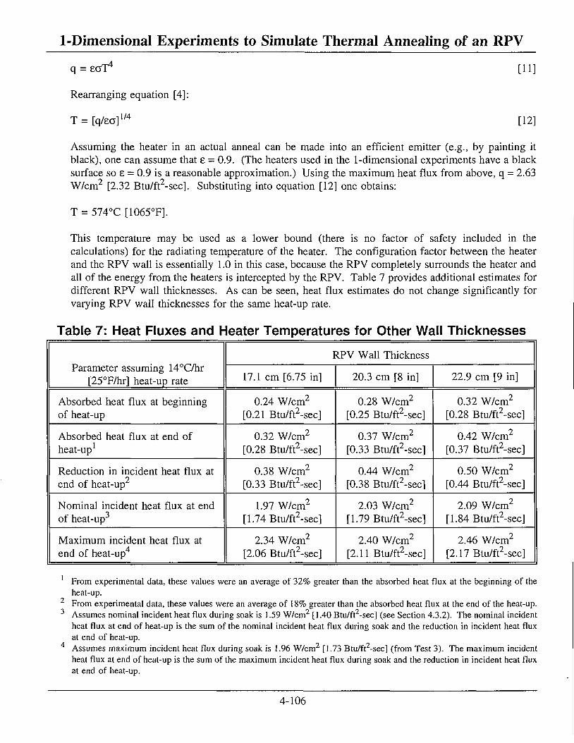
1-Dimensional Experiments to Simulate Thermal Annealing of an RPV = 8GT 4 [11]
Rearranging equation [4]:
T = [q/eo] 1/4 [12]
Assuming the heater in an actual anneal can be made into an efficient emitter (e.g., by painting it black), one can assume that e = 0.9. (The heaters used in the 1-dimensional experiments have a black surface so £ = 0.9 is a reasonable approximation.) Using the maximum heat flux from above, q = 2.63 W/cm [2.32 Btu/ft -sec]. Substituting into equation [12] one obtains:
T = 574°C [1065°F].
This temperature may be used as a lower bound (there is no factor of safety included in the calculations) for the radiating temperature of the heater. The configuration factor between the heater and the RPV wall is essentially 1.0 in this case, because the RPV completely surrounds the heater and all of the energy from the heaters is intercepted by the RPV. Table 7 provides additional estimates for different RPV wall thicknesses. As can be seen, heat flux estimates do not change significantly for varying RPV wall thicknesses for the same heat-up rate.
Table 7: Heat Fluxes and Heater Temperatures for Other Wall Thicknesses
Parameter assuming 14°C/hr [25°F/hr] heat-up rate
RPV Wall Thickness Parameter assuming 14°C/hr
[25°F/hr] heat-up rate 17.1 cm [6.75 in] 20.3 cm [8 in] 22.9 cm [9 in]
Absorbed heat flux at beginning of heat-up
0.24 W/cm2
[0.21 Btu/ft2-sec] 0.28 W/cm2
[0.25 Btu/ft2-sec] 0.32 W/cm2
[0.28 Btu/ft2-sec]
Absorbed heat flux at end of heat-up
0.32 W/cm2
[0.28 Btu/ft2-sec] 0.37 W/cm2
[0.33 Btu/ft2-sec] 0.42 W/cm2
[0.37 Btu/ft2-sec]
Reduction in incident heat flux at end of heat-up
0.38 W/cm2
[0.33 Btu/ft2-sec] 0.44 W/cm2
[0.38 Btu/ft2-sec] 0.50 W/cm2
[0.44 Btu/ft2-sec]
Nominal incident heat flux at end of heat-up
1.97 W/cm2
[1.74 Btu/ft2-sec] 2.03 W/cm2
[1.79 Btu/ft2-sec] 2.09 W/cm2
[1.84Btu/ft2-sec]
Maximum incident heat flux at end of heat-up
2.34 W/cm2
[2.06 Btu/ft2-sec] 2.40 W/cm2
[2.11 Btu/ft2-sec] 2.46 W/cm2
[2.17 Btu/ft2-sec]
From experimental data, these values were an average of 32% greater than the absorbed heat flux at the beginning of the heat-up. From experimental data, these values were an average of 18% greater than the absorbed heat flux at the end of the heat-up. Assumes nominal incident heat flux during soak is 1.59 W/cm2 [1.40 Btu/ft -sec] (see Section 4.3.2). The nominal incident heat flux at end of heat-up is the sum of the nominal incident heat flux during soak and the reduction in incident heat flux at end of heat-up. Assumes maximum incident heat flux during soak is 1.96 W/cm2 [1.73 Btu/ft -sec] (from Test 3). The maximum incident heat flux at end of heat-up is the sum of the maximum incident heat flux during soak and the reduction in incident heat flux at end of heat-up.
4-106
1-Dimensional Experiments to Simulate Thermal Annealing of an RPV 4.10.7 Concrete Wall Temperatures
• On Test 2, the maximum temperature reached on the concrete wall was on TCI: 40°C [104°F], but all 8 other TCs were clustered around 30°-35°C [86°-95°F].
• . On Test 3, the maximum temperature reached on the concrete wall was on TCI: 40°C [104°F], but all 8 other TCs were clustered around 28°-32°C [82°-90°F]. On Test 7, the repeat of Test 3, the maximum temperature reached on the concrete wall was on TCI: 44°C [111°F], but all 8 other TCs were clustered around 25°-33°C [77°-91°F].
• On Test 4, the maximum temperature reached on the concrete wall was on TCI: 42°C [108°F], but all 8 other TCs were clustered around 28°-33°C [82°-91°F].
4.10.8 Power Input to Heaters
• During all tests, the bottom bank of heaters consumed the most power (about 16 kW during the soak), while the middle bank consumed the least (about 1 kW during the soak on Tests 2, 3, and 4, but up to about 2.5 kW on Test 7). The top bank consumed about 5-6 kW during the soak on Tests 2-4, but about 4 kW on Test 7. These data suggest that, in a real anneal, power to the middle heaters will be less than power to the top and bottom. In addition, if there is a large heat sink nearby (e.g., nozzle and reactor coolant system piping) the heater input required will be much greater.
4.10.9 Measurement Errors/Uncertainties
• Thermocouple errors stemming from the mounting method used (intrinsic versus sheathed) were as much as +5°C [+9°F]. Depending on the design, TC mounting method errors could be much larger than these values.
• Thermocouple measurement errors could be up to ±3.6%, but are likely much less, e.g., ±1%.
• Pyrheliometer heat flux measurement uncertainties are +6.3%, -9.3%.
• SODDIT heat flux estimation uncertainties depend on temperature uncertainties. For every 1.1 °C [2°F] uncertainty in temperature the absorbed heat flux uncertainty is about 0.0074 W/cm2 [0.0065Btu/ft2-sec].
• Air flow measurement uncertainties are nominally ±20%, but during periods of large fluctuation, the uncertainty may be up to ±30%.
4-107

1-Dimensional Experiments to Simulate Thermal Annealing of an RPV 4.11 Comparison with NUREG/CR-4212, "In-PIace Thermal Annealing of Nuclear Reactor
Pressure Vessels"
NUREG/CR-4212 contains an in-depth thermal and structural analysis of a thermal anneal in Appendix C, titled "An Evaluation of the Consequences of an In-PIace Anneal of a PWR Reactor Vessel." The thermal and structural analysis was performed by Combustion Engineering (CE), Inc., on a CE RPV 437 cm [172 in] inside diameter, 21.9 cm [8.625 in] thick with a 7.9 cm [0.313 in] thick stainless steel cladding. The temperature profile consisted of a heat-up and cool-down rate of 14°C/hr [25°F/hr] and a soak at 454°C [850°F], the same as Test 2 in this report. It would be of benefit to compare several areas of the NUREG with the experimental results in this report. Specifically, details of the absorbed heat flux into the RPV and the axial absorbed heat flux variations will be discussed.
The NUREG analysis assumed five (5) axial regions with variable heat flux control. Results show that the very top and bottom regions required much larger heat flux to maintain a constant RPV temperature of 454°C [850°F] than did the middle three (3) regions. This result is consistent with the results obtained in the experiments described in this report.
Figure 3 in Appendix C (page C-9) of the NUREG showed hot wall heat flux: "the actual heat flux input to the vessel wall," which is the same as the "absorbed heat flux" presented in this report. After taking into account that the time scale is compressed, the shape of the plots in the figure are similar to typical absorbed heat flux plots in this report (e.g., Figures 35 and 58). However, the maximum absorbed heat flux reported in Region 5 was 2677 Btu/hr-ft2 (0.85 W/cm2 [0.74 Btu/ft2-sec]), about twice as large as the maximum reported in Table 7 in this report. This comparison accounts for the different RPV wall thickness, 0.32 W/cm2 [0.28 Btu/ft2-sec] for 17.1 cm [6.75 in] thick wall in this report increases to about 0.40 W/cm2 [0.36 Btu/ft2-sec] for 21.9 cm [8.625 in] thick wall in the NUREG. In addition, the absorbed heat flux in the NUREG during the 454°C [850°F] soak did not drop to zero in Region 5. The experimental data presented in this report apply only to the portion of the RPV where the heat transfer is 1-dimensional (i.e., in the middle 3 regions of the CE model). Therefore, the absorbed heat flux in Region 5 (very top of the heated zone) should be greater than that in the middle, and would be non-zero during the soak due to axial conduction in the RPV.
Figure 3 also shows a heat flux plot in Region 3, in the very middle of the RPV. The maximum flux reported in that region is 1497 Btu/ft2-hr, or 0.47 W/cm2 [0.42 Btu/ft2-sec] at the end of the heat-up. From Table 7 in this report one can estimate the absorbed heat flux at the end of the heat-up to be about 0.40 W/cm2 [0.36 Btu/ft2-sec] for a 21.9 cm [8.625 in] thick RPV wall, or about 15% below the value (0.47 W/cm2 [0.42 Btu/ft2-sec]) reported in the NUREG. Due to slight differences in the CE model and the Sandia experimental setup, the 15% difference is understandable.
Therefore, results regarding heat flux reported in NUREG/CR-4212 and this report are generally consistent. Other results were not easily compared and so are not discussed further.
4-108
1-Dimensional Experiments to Simulate Thermal Annealing of an RPV
5. Conclusions and Other Information The objective of this work was to provide experimental heat transfer boundary condition and reactor
pressure vessel (RPV) section thermal response data that can be used to benchmark computer codes that simulate thermal annealing of RPVs. This specific project was designed to provide the Electric Power Research Institute (EPRI) with experimental data that could be used to support the development of a model to simulate thermal annealing. A secondary benefit is to provide additional experimental data (e.g., thermal response of concrete reactor cavity wall) that could be of use in an annealing demonstration project. Significant conclusions are as follows:
1. Temperature uniformity on the heated face of the RPV section during the soak was very good for all tests: Test 2 was better than ±5%, Test 3 was better than 4%, and Test 4 was better than ±3%.
2. Through-wall temperature differences at the end of the heat-up portion were greater for higher heat-up rates (maximum of 18°-37°C [32°-67°F]), but were essentially the same during the hold period (4°-21°C [7°-38°F]).
3. There were small but noticeable temperature differences between the response of the weld material and the base metal. However, the differences in response are small (maximum of ±4.5°C [± 8.1°F]) and will likely not contribute to significant thermal stresses.
4. Incident heat flux for Test 3, which had the fastest heat-up rate, showed the highest heat flux (2.63 W/cm2 [2.32 Btu/ft2-sec]). Test 4, with the slowest heat-up rate, showed the lowest incident heat flux. However, the soak heat flux values for all 3 tests are essentially identical (between 1.5-1.9 W/cm2 [1.3-1.7 Btu/ft2-sec]). Predicted values of incident heat flux compared favorably with experimental values.
5. The measured absorbed heat fluxes agreed with predicted values at the beginning of the heat-up. However, the measured absorbed heat fluxes kept slowly rising after the initial sharp rise while the predicted values were constant. Absorbed heat flux on all tests dropped to zero during the soak.
6. For a heater designer, one may assume a maximum heater output adjusted for RPV wall thickness to estimate a heater temperature.
7. The maximum temperature on the concrete wall was about 44°C [111°F] for a single TC, but most of the TCs were clustered around 25°-35°C [77°-95°F].
8. Power input to the middle bank heaters was consistently less than either the top or bottom bank during the soak.
9. The thermocouple mounting method could introduce a bias into the RPV temperature measurement, causing the indication to be higher than the RPV temperature.
10. Depending on the RPV temperature measurement error and the magnitude of the uniformity on the RPV surface, one may choose to increase the soak temperature above 454°C [850°F] (Appendix A).
11. Results regarding heat flux in this report are consistent with those presented in NUREG/CR-4212.
5-1

1-Dimensional Experiments to Simulate Thermal Annealing of an RPV
6. References 1. W. L. Server, T. J. Griesbach, E. L. Kennedy, C. S. Venkatakrishnan, "Reactor Pressure
Vessel Life Assurance Decisions," Service Experience and Life Management: Nuclear, Fossil, and Petrochemical Plants, PVP-Vol. 261, 1993 Pressure Vessels and Piping Conference, American Society of Mechanical Engineers, New York, July 1993, pp. 89-94.
2. B. MacDonald, "Post-Irradiation Annealing Recovery of Commercial Pressure Vessel Steels," Effects of Radiation on Materials: Twelfth International Symposium, ASTM STP 870, F. A. Garner and J. S. Perrin, Eds., American Society for Testing and Materials, Philadelphia, 1985, pp. 972-978.
3. T. R. Mager, Feasibility of and Methodology for Thermal Annealing an Embrittled Reactor Vessel, EPRI NP-2712, Vol. 2, Electric Power Research Institute, November 1992.
4. A. Fabry, et al., "Annealing of the BR3 Reactor Pressure Vessel," Proceedings of the U.S. Nuclear Regulatory Commission Twelfth Water Reactor Safety Research Information Meeting, Vol. 4 - Materials Engineering Research, NUREG/CP-0058, U.S. Nuclear Regulatory Commission, January 1985, pp. 144-175.
5. N. M. Cole, T. Friderichs, "Report on Annealing of the Novovoronezh Unit 3 Reactor Vessel in the USSR," NUREG/CR-5760, U.S. Nuclear Regulatory Commission, Washington, D.C., July 1991.
6. U. Potapovs, J. R. Hawthorne, C. Z. Serpan, Nuclear Applications, Vol. 5, No. 6, 1968, pp. 389-409.
7. T. R. Mager, R. G. Lott, Thermal Annealing of an Embrittled Reactor Vessel, Feasibility and Methodology, EPRI NP-6113-SD, Electric Power Research Institute, January 1989.
8. EPRI Report NP-2493, "Development of a Generic Procedure for Thermal Annealing an Embrittled Reactor Pressure Vessel Using a Dry Annealing Method," Project 1021-1, prepared by Westinghouse Electric Corporation, July 1982.
9. Analytical Heat Diffusion Theory, by A.V. Luikov, Edited by James P. Hartnett, Academic Press, New York, 1968, p. 9.
10. "An Error Analysis of Thermocouple Measurements in the Radiant Heat Facility," Sandia Report SAND80-2655, by J.T. Nakos and B.G. Strait, December 1980.
11. Thermophysical Properties of Matter, Volume 1, Thermal Conductivity, Metallic elements and Alloys, Y.S. Touloukian, R.W. Powell, C.Y. Ho and P.G. Klemens, IFI/Plenum Data Corp., New York, 1970.
12. ASM Metals Reference Book, Second Edition, American Society for Metals, 1983.
13. Standard Oil Engineered Materials Company, Fibers Division, Niagara Falls, NY, Product Specifications for "Fiberfrax Durablanket," August 1987.
6-1
1-Dimensional Experiments to Simulate Thermal Annealing of an RPV 14. Principles of Heat Transfer by Frank Kreith, 3 edition, Intext Educational Publishers,
1973, Figure 5-22, p. 249.

1-Dimensional Experiments to Simulate Thermal Annealing of an RPV
Appendix A - RPV Temperature Variation: Effect on Control Temperature
Figure A-l shows a histogram of RPV heated face temperature data during two time periods (beginning and end of soak) during the soak for Tests 2, 3, 4, and 7. As can be seen, the distribution looks similar to a Gaussian distribution with the mean at about 454°C [850°F]. The mean temperature was 453.31°C [847.96°F] and the standard deviation was 6.9TC [12.44°F]. Figure A-2 compares all the data points (*) with a Gaussian (Normal) distribution (solid line). The data compare well.
The effect of the Gaussian distribution of temperature on the RPV surface can be seen in Figure A-3. At a setpoint/soak temperature of 454°C [850°F], 50% of the RPV was below the setpoint and 50% above. Assuming the temperature variation during an actual anneal follows a Gaussian distribution and there is some lower threshold temperature below which the RPV will not be effectively annealed, one may choose to raise the setpoint temperature to ensure that a large fraction of the RPV is above the threshold temperature. For example, assuming the threshold temperature is 454°C [850°F] and one wants to ensure that 95% of the RPV is above that threshold, from Figure A-3 the setpoint temperature should be about 465°C [869°F].
In addition, if one assumes (from Section 4.8) there are TC mounting method errors that would cause the TCs to indicate higher temperatures than the RPV surface, one may also choose to increase the setpoint further. For example, if TC mounting method errors from Section 4.8 are used (4°C [7°F]), one may choose to raise the setpoint by an additional 4°C [7°F], up to 475°C [887°F]. Note: the TC mounting method error should be consistent with the measurement technique used in the actual anneal, not the laboratory condition used in these experiments.
A-l

1-Dimensional Experiments to Simulate Thermal Annealing of an RPV
wm
09 OS Of 0£ 0£
s^unoQ
0L ~i
0
o i - 00
o
o
•a ^1-
ning
and
End
of
So
o <D ning
and
End
of
So
( O _ c f- 3 GO
•+-> <D D CQ L_ 4 - *
<D ca Q_
E Q 0 <u
i— I-I 3
•4—1
o ^ l-<
l O D G, •NT ^
Hea
ted
Face
Ter
n
o > <sf- OH
•N}-gu
re A
-1.
R
HH
A-2

i*>i,*;
> i
V
i_ D D i_ 0) CL
E 0
Q_
00
d
CD
d
d
CM
d
o d
Mean: 453.31°C [847.96°F] Sigma: 6.91°C [12.44°F]
* *-
<'•>/'! 430 440 450 460 470 480 T (C)
Figure A-2. Comparison of RPV Heated Face Temperature with Gaussian Distribution.
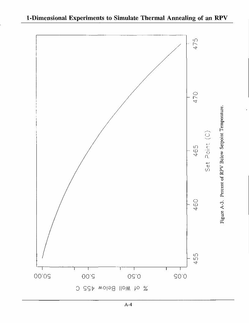
1-Dimensional Experiments to Simulate Thermal Annealing of an RPV
LO
o
o
o CD
LO lO
<L>
u,
1)
o
LD c CD -xt- P
oi
elow
•+-> PQ a> >
CO a-Pi
a <u o
OH
CO I
< 1)
00 • •-H
00'09 00"9 09"0 so'o 0 9917 Mopg I P M P %
A-4
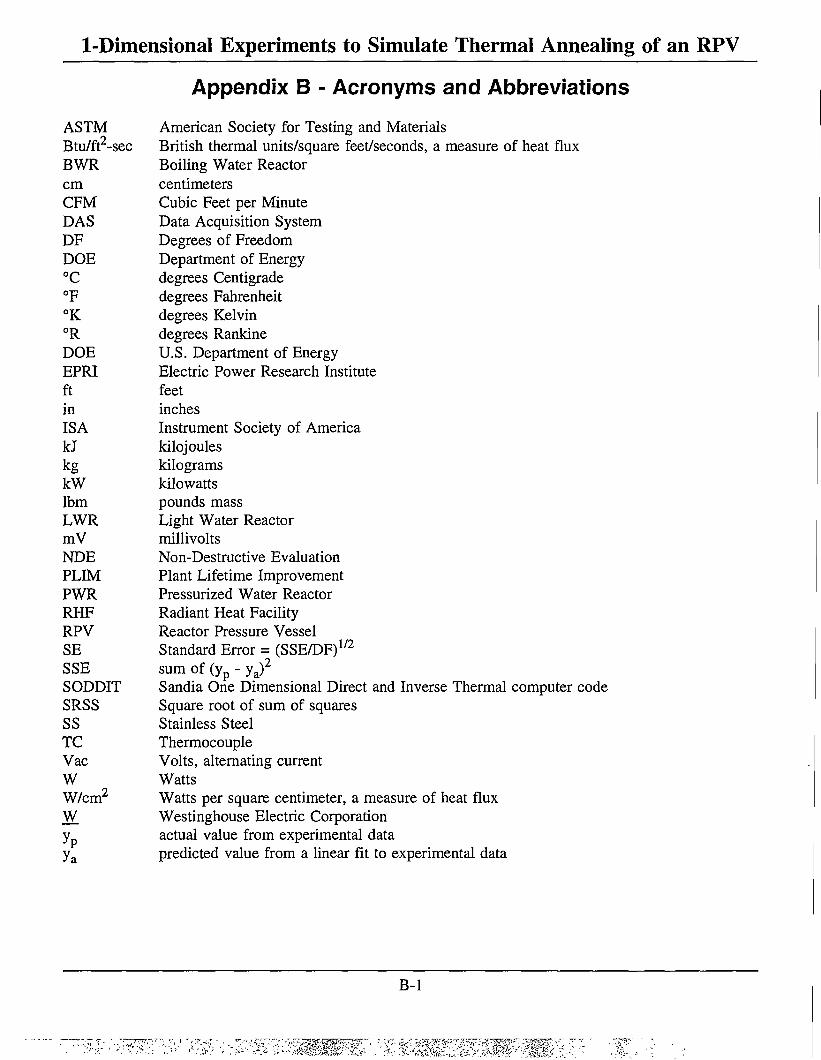
1-Dimensional Experiments to Simulate Thermal Annealing of an RPV
Appendix B - Acronyms and Abbreviations ASTM American Society for Testing and Materials Btu/ft2-sec British thermal units/square feet/seconds, a measure of heat flux BWR Boiling Water Reactor cm centimeters CFM Cubic Feet per Minute DAS Data Acquisition System DF Degrees of Freedom DOE Department of Energy °C degrees Centigrade °F degrees Fahrenheit °K degrees Kelvin °R degrees Rankine DOE U.S. Department of Energy EPRI Electric Power Research Institute ft feet in inches ISA Instrument Society of America kJ kilojoules kg kilograms kW kilowatts lbm pounds mass LWR Light Water Reactor mV millivolts NDE Non-Destructive Evaluation PLIM Plant Lifetime Improvement PWR Pressurized Water Reactor RHF Radiant Heat Facility RPV Reactor Pressure Vessel SE Standard Error = (SSE/DF)1 7 2
SSE sum of (y p - y a ) 2
SODDIT Sandia One Dimensional Direct and Inverse Thermal computer code SRSS Square root of sum of squares SS Stainless Steel TC Thermocouple Vac Volts, alternating current W Watts W/cm2 Watts per square centimeter, a measure of heat flux W Westinghouse Electric Corporation y P actual value from experimental data y a
predicted value from a linear fit to experimental data
B-l
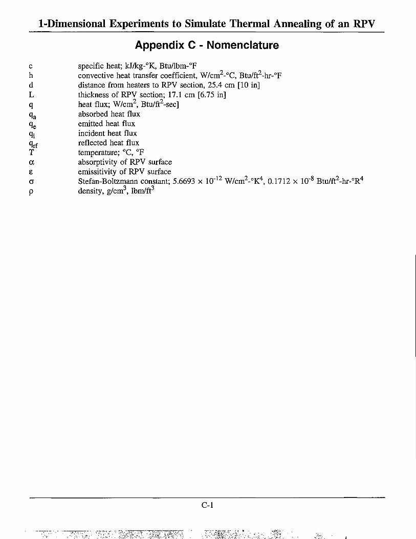
1-Dimensional Experiments to Simulate Thermal Annealing of an RPV
Appendix C - Nomenclature c specific heat; kJ/kg-°K, Btu/lbm-°F h convective heat transfer coefficient, W/cm2-°C, Btu/ft2-hr-°F d distance from heaters to RPV section, 25.4 cm [10 in] L thickness of RPV section; 17.1 cm [6.75 in] q heat flux; W/cm2, Btu/ft2-sec] q a
absorbed heat flux q e
emitted heat flux q* incident heat flux qrf reflected heat flux T temperature; °C, °F a absorptivity of RPV surface e emissitivity of RPV surface a Stefan-Boltzmann constant; 5.6693 x 10" 1 2 W/cm2-°K4, 0.1712 x 10"8 Btu/ft2-hr-°R4
P density, g/cm3, lbm/ft3
C-l

DISTRIBUTION Category UC-523 (91 copies)
Department of Energy
Dennis Harrison (2 copies) U.S. Department of Energy, NE-451 19901 Germantown Road Germantown, MD 20852
Charles Thompson U.S. Department of Energy, NE-451 19901 Germantown Road Germantown, MD 20852
Sterling Franks, III U.S. Department of Energy, NE-451 19901 Germantown Road Germantown, MD 20852
EPRI
Robert Carter (2 copies) EPRI Component Reliability Center 1300 Harris Boulevard Charlotte, NC 28262
Jack Lance EPRI Component Reliability Center 1300 Harris Boulevard Charlotte, NC 28262
Larry Becker EPRI Component Reliability Center 1300 Harris Boulevard Charlotte, NC 28262
John Carey Electric Power Research Institute 3412 Hillview Avenue Palo Alto, CA 94303
Robin Jones Electric Power Research Institute 3412 Hillview Avenue Palo Alto, CA 94303
EPRI Life Cycle Management Subcommittee
Barth Doroshuk Baltimore Gas & Electric Calvert Cliffs Route 4 South Lusby, MD 20657
Richard Remshaw Consolidate Edison Co. of New York 4 Irving Place, Rm. 1238 New York, NY 10003
Greg Robison Duke Power Company, EC09F 422 South Church Street P.O. Box 1006 Charlotte, NC 28201-1006
W.F. Mashburn Entergy Operations, Inc. River Bend Station 5485 U.S. Highway 61 St. Francisville, LA 70775
Roger Murgatroid Crystal River Nuclear Plant 15760 W. Power Line Street (MC-NA2G) Florida Power Corporation Crystal River, FL 34429
Robert Locke GPU Nuclear 1 Upper Pond Road Parsippany, NJ 07054
Karl Jacobs New York Power Authority 123 Main Street White Plains, NY 10601
Don Eggett Commonwealth Edison Co. 1400 Opus Place, Suite 300 Downer Grove, IL 60515
DIST-1

Ray McNamara Pennsylvania Power & Light Company Two North Ninth Street Allentown, PA 18101
Jim Perrin Public Service Electric & Gas Co. P.O. Box 236, N32 Hancocks Bridge, N.J. 08038
Jose Perez Southern California Edison 23 Parker Ave. Irvine, CA 92718
John Giddens Southern Nuclear Operating Co. 40 Inverness Center Parkway (35242) P.O. Box 1295 Birmingham, AL 35201-1295
Jim Chardos Tennessee Valley Authority BR 4G-C 1101 Market Street Chattanooga, TN 37402
John Swailes Washington Public Power Supply System 3000 George Washington Way MD 927M Richland, Washington 99352
Chuck Krause Wisconsin Electric Power Company 231 West Michigan P.O. Box 2046 Milwaukee, Wl 53201
Nuclear Regulatory Commission
Charles Serpan U.S. Nuclear Regulatory Commission 5650 Nicholson Lane, M.S. 217C NL/S Rockville, MD 20852
Allen Hiser, Jr. U.S. Nuclear Regulatory Commission 5650 Nicholson Lane, M.S. 217C NL/S Rockville, MD 20852
Mike Mayfield U.S. Nuclear Regulatory Commission 5650 Nicholson Lane, M.S. 217C NL/S Rockville, MD 20852
Al Taboada U.S. Nuclear Regulatory Commission 5650 Nicholson Lane, M.S. 217C NL/S Rockville, MD 20852
Keith Wichman U.S. Nuclear Regulatory Commission 11555 Rockville Pike, M.S. 7D4 Rockville, MD 20852
NEI
Kurt Cozens NEI 1776 Eye Street, N.W., Suite 300 Washington, D.C. 20006-2496
National Labs
A. G. Ware EG&G Idaho Post Office Box 1625 Idaho Falls, ID 83415-3503
Shafik Iskander Oak Ridge National Laboratory Post Office Box 2008 Oak Ridge, TN 37831
R. K. Nanstad Oak Ridge National Laboratory Post Office Box 2008 Oak Ridge, TN 37831
Mikhail Sokolov Oak Ridge National Laboratory Post Office Box 2008 Oak Ridge, TN 37831
DIST-2

F. Simonen Battelle Pacific Northwest Labs Post Office Box 999 Richland, WA 99352
NSSS Vendors
Dave Ayers ABB Combustion Engineering 1000 Prospect Hill Road Windsor, CT 06095-0500
P. Hijeck ABB Combustion Engineering 1000 Prospect Hill Road Windsor, CT 06095-0500
E. A. Siegel ABB Combustion Engineering 1000 Prospect Hill Road Windsor, CT 06095-0500
H. W. Behnke B&W Nuclear Service Company Post Office Box 10935 Lynchburg, VA 24506-0935
F. R. Burke B&W Nuclear Service Company Post Office Box 10935 Lynchburg, VA 24506-0935
Bill Clark Westinghouse Electric Company 1310 Beulah Road Pittsburgh, PA 15235
Tom Dent Westinghouse Electric Corporation P.O. Box 158 Madison, PA 15663-0355
David Howell Westinghouse Electric Company Post Office Box 355 Pittsburgh, PA 15230-0355
Tom Mager Westinghouse Electric Company Post Office Box 2728 Pittsburgh, PA 15230
Cynthia Pezze Westinghouse Electric Corporation P.O. Box 355 Pittsburgh, PA 15230
Rick Rishel Westinghouse Electric Company Post Office Box 355 Pittsburgh, PA 15230-0355
John Spitznagel Science & Technology Center Westinghouse Electric Corporation 1310 Beulah Road Pittsburgh, PA 15235
Lee Tunon-Sanjur Westinghouse Electric Corporation P.O. Box 355 Pittsburgh, PA 15230-0355
Utilities
T. Satyan Sharma American Electric Power One Riverside Plaza Columbus, OH 43216
Mike Melton Arizona Public Service Company 411 North Central Ave. Station 1796 Phoenix, AZ 85072
Robert Hardies Calvert Cliffs Nuclear Power Plant 1650 Calvert Cliffs Parkway Lusby, MD 20657
Grant Chappell Carolina Power & Light Co. P.O. Box 1551 Raleigh, NC 27602
DIST-3

Charles H. Griffin Carolina Power & Light P.O. Box 1551 Raleigh, NC 27602-1551
Alex G. Panagos Commonwealth Edison Company Suite 400 1400 Opus Place Downers Grove, IL 60515
Russell J. Tamminga Commonwealth Edison Company Suite 400 1400 Opus Place Downers Grove, IL 60515
David P. Hoffman Vice President, Nuclear Operations Consumers Power Co. 212 W. Michigan Ave. Jackson, Ml 49201
Thomas Buczwinski Consumers Power Company Palisades Station 27780 Blue Star Highway Covert, Ml 49085
Jack Hanson Consumers Power Company Palisades Nuclear Plant 27780 Blue Star Hwy Covert, Ml 49043
John Kneeland Consumers Power Company Palisades Station 27780 Blue Star Hwy, Rm P-26-411A Covert, Ml 49043
Jeff Gilreath Duke Power Company 526 South Church Street, MC EC09O Post Office Box 1006 Charlotte, NC 28201
Greg Kammerdeiner Director, Materials and Standards Duquesne Light Company Beaver Valley P.O. Box 184 Shippingport, PA 15077
Dan Fouts Entergy Operations Arkansas Nuclear One, Unit 1 P.O. Box 137G Highway 64 West, GSB-3WEST Russelville, AK 72801
Karen Head Entergy Operations Arkansas Nuclear One, Unit 2 P.O. Box 137G Highway 64 West, GSB-3WEST Russelville, AK 72801
Jai S. Brihmadesam Entergy Operations 1340 Echelon Parkway Jackson, MS 39213
Steve Collard Florida Power & Light 700 Universe Boulevard P.O. Box 14000 Juno Beach, FL 33408
Vince Roppel Crystal River Nuclear Plant Florida Power Corporation P.O. Box 1240 Crystal River, FL 34429
Dave Miskiewicz Florida Power Corporation P.O. Box 14042, MAC C2M St. Petersburg, FL 33733-4042
Terry Sides Southern Nuclear Operating Co. P.O. Box 1295 Birmingham, AL 35201-1295
DIST-4

Robin Dyle Southern Nuclear Operating Co. P.O. Box 1295 Birmingham, AL 35201-1295
George L. Lehmann GPU Nuclear 100 Interpace Parkway Parsippany, NJ 07054
Chung He Chen GPU Nuclear 100 Interpace Parkway Parsippany, NJ 07054
Chris Freer Indiana Michigan Power D.C. Cook Nuclear Power Plant 1 Cook Place Bridgeman, Ml 49106
B. Ralph Sylvia Executive Vice President, Nuclear Niagara Mohawk Power Corp. 300 Erie Blvd. W. Syracuse, NY 13202
Matthew L. Paquette Northeast Utilities P.O. Box 270 Hartford, CT 06141
J. Haseltine Northeast Utilities Connecticut Yankee Atomic Power Haddam Neck Plant 362 Injun Hollow Road East Hampton, Conn. 06424
Matt Kupinski Northeast Utilities Post Office Box 270 Hartford, CT 06141
Kevin Holthaus Omaha Public Power District Energy Plaza 444 S. 16th Street Mall Omaha, NE 68102
Bill Weber Omaha Public Power District Energy Plaza 444 S. 16th Street Mall Omaha, NE 68102
Marcus Guinn Omaha Public Power District Energy Plaza 444 S. 16th Street Mall Omaha, NE 68102
Phil Brashear Pacific Gas and Electric Co. 333 Market San Francisco, CA 94177
Robert McDevitt Pacific Gas and Electric Co. 77BeaIeSt. - Room 1414 San Francisco, CA 94106
Mike Sullivan Pacific Gas & Electric Company 3400 Crow Canyon Road San Ramon, CA 94583
Mahesh R. Danak Public Service Electric & Gas Co. Hope Creek Power Station P.O. Box 236 Hancocks Bridge, NJ 08038
Ron Jaquin Rochester Gas & Electric Corp. 89 East Avenue Rochester, NY 14649-0001
DIST-5

Keith Reeser Southern California Edison Mail Drop X345 23 Parkers Street Irvine, CA 92718
Dana R. Couch Tennessee Valley Authority 1101 Market St. LP 4F Chattanooga, TN 37402
John Harrell Virginia Power Company Innsbrook Technical Center, M/S IN3SW 5000 Dominion Blvd. Glen Allen, VA 23060
Joe Hegner Virginia Power Company Innsbrook Technical Center, M/S IN2E 5000 Dominion Blvd. Glen Allen, VA 23060
James R. Pfefferle, P.E. Wisconsin Electric Power Co. P.O. Box 2046 Melwaukee, Wl 53201
Ronda Fergusson Wisconsin Public Service Corp. 700 N. Adams P.O. Box 19002 Green Bay, Wl 54307
Chuck Tomes Wisconsin Public Service Corp. 600 N. Adams Green Bay, Wl 54302
International
Albert Fabry SCK-CEN Boeretang 200 B-2400, Mol Belgium
Milan Brumovsky Nuclear Research Institute Rez pic 250 68 Rez Czech Republic
L. Myrddin Davies 176 Cumnor Hill Oxford Oxon 0X2 9PJ England
Tapio M. Planman VTT Manufacturing Technology P.O. Box 1704 VTT FIN-02044 Finland
Matti Valo VTT Manufacturing Technology P.O. Box 17042 VTT FIN-02044 Finland
Ludwig Stumpfrock Staatliche Materialprufungsanstalt Pfaffenwaldring 32 70569 Stuttgart Germany
Sergei Bougaenko R&D Institute of Power Engineering Minatom (MAE) P.O. Box 788, Moscow, 101000 Russia
Yuri G. Dragunov OKB "Gidropress" Ordzhonikidze 21 142103, Podolsk, Moskow reg. Russia
G. P. Karzov Central Research Institute "Prometey" 193167, St. Petersburg Russia
DIST-6
A. M. Kryukov Kurchatov Institute Kurchatov Square, 1 123182 Moscow, Russia
Sergei C. Morozov VNIIAES Ferganskaya St. 25 Moscow, Russia
Michael F. Rogov GIDROPRESS Ozdzhowikidze 21 Podolsk, Russia
Others
Neil Irvine AEA O'Donnell, Inc. 241 Curry Hollow Road Pittsburgh, PA 15236
Janek Porowski AEA O'Donnell, Inc. 241 Curry Hollow Road Pittsburgh, PA 15236
Russ Cipolla APTECH Engineering Services 1282 Reamwood Avenue Sunnyvale, CA 94089
Tim Griesbach ATI Consulting 2010 Crow Canyon Place, Suite 140 San Ramon, CA 94583
William Server ATI Consulting 2010 Crow Canyon Place, Suite 140 San Ramon, CA 94583
Bill Hopkins Bechtel Power Corporation 9801 Washingtonian Blvd. Gaithersburg, MD 29878-5356
Glenn Campbell (2 copies) Cooperheat 1021 Centennial Ave. Piscataway, NJ 08854
Wayne A. Pavinich Grove Engineering 9040 Executive Park Drive Suite 218 Knoxville, TN 37923
Noman Cole MPR Associates 320 King Street Alexandria, VA 22314-3238
Tom Friderichs MPR Associates 320 King Street Alexandria, VA 22314-3238
Alex Zarechnak MPR Associates 320 King Street Alexandria, VA 22314-3238
Ron Gamble Sartrex Corporation 1700 Rockville Pike, Suite 400 Rockville, MD 20852
Pete Riccardella Structural Integrity Associates, Inc. 3150 Almaden Expressway, Suite 226 San Jose, CA95118
G. Robert Odette Dept. of Chemical & Nuclear Eng. University of California Santa Barbara, CA 93106
DIST-7

Internal
MS 0507 Kathleen McCaughey (2700) MS 0653 Bobby Strait (3522) MS 0826 Ben Blackwell (1553) MS 0835 Bruce Bainbridge (1513) MS 1135 Mark Garrett (2761) MS 1135 Russ Acton (2761) MS 1135 Walt Gill (2761) MS 1135 Bill Jacoby (2761) MS 1135 Ned Keltner (2761) MS 1135 David Schulze (2761) MS 0736 Nestor Ortiz (6400) MS 0741 Ajoy Moonka (6471) MS 0741 John Clauss (6471) MS 0741 Jim Nakos (6471) - 10 copies MS 0741 Stan Rosinski (6471) - 5 copies MS 0899 Technical Library (13414) -
5 copies MS 0619 Technical Publications (13416) MS 0100 Document Processing for
DOE/OSTI (7613-2) -10 copies MS 9018 Central Tech. Files (8523-2)
DIST-8