1

Code Compression

Motivations Data compression techniques Code compression options and methods Comparison

2

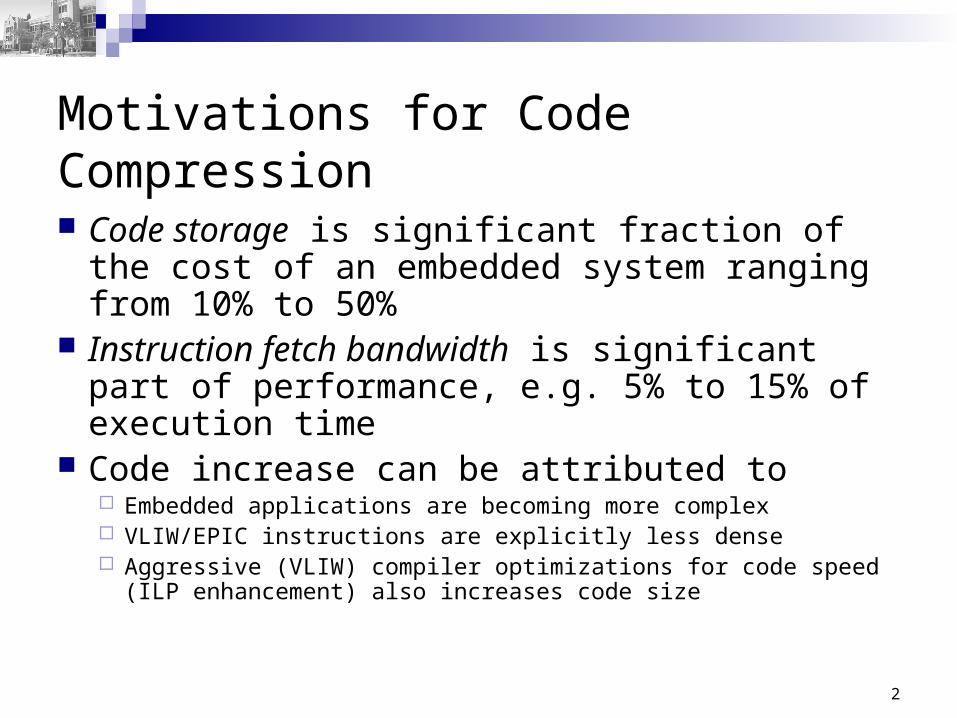
Motivations for Code Compression

Code storage is significant fraction of the cost of an embedded system ranging from 10% to 50%

Instruction fetch bandwidth is significant part of performance, e.g. 5% to 15% of execution time

Code increase can be attributed to Embedded applications are becoming more complex VLIW/EPIC instructions are explicitly less dense Aggressive (VLIW) compiler optimizations for code speed

(ILP enhancement) also increases code size

3

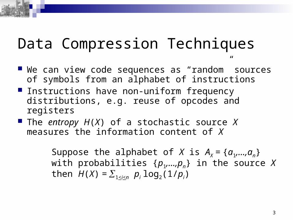
Data Compression Techniques

We can view code sequences as “random” sources of symbols from an alphabet of instructions

Instructions have non-uniform frequency distributions, e.g. reuse of opcodes and registers

The entropy H(X) of a stochastic source X measures the information content of X

Suppose the alphabet of X is AX = {a1,…,an}with probabilities {p1,…,pn} in the source Xthen H(X) = 1<i<n pi log2(1/pi)

4

Examples

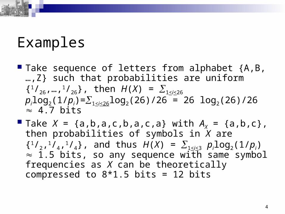
Take sequence of letters from alphabet {A,B,…,Z} such that probabilities are uniform {1/26,…,1/26}, then H(X) = 1<i<26 pilog2(1/pi)=1<i<26log2(26)/26 = 26 log2(26)/26 4.7 bits

Take X = {a,b,a,c,b,a,c,a} with AX = {a,b,c}, then probabilities of symbols in X are {1/2,1/4,1/4}, and thus H(X) = 1<i<3 pilog2(1/pi) 1.5 bits, so any sequence with same symbol frequencies as X can be theoretically compressed to 8*1.5 bits = 12 bits

5

Huffman Encoding

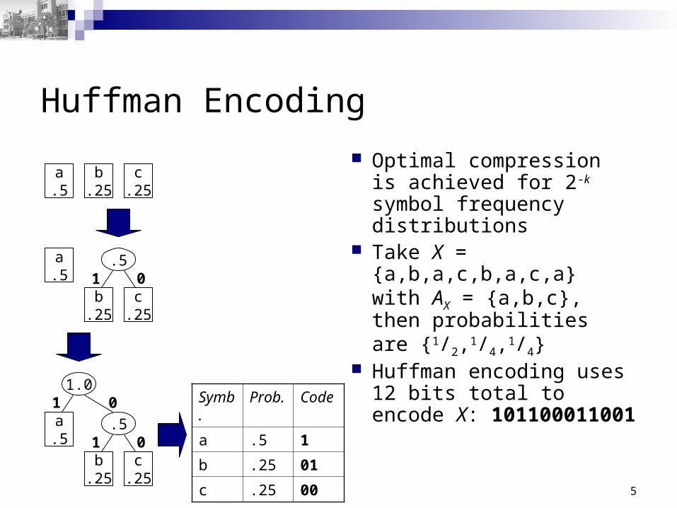
Optimal compression is achieved for 2-k symbol frequency distributions

Take X = {a,b,a,c,b,a,c,a} with AX = {a,b,c}, then probabilities are {1/2,1/4,1/4}

Huffman encoding uses 12 bits total to encode X: 101100011001

a.5

b.25

c.25

a.5

b.25

c.25

.51 0

a.5

b.25

c.25

.51 0

1.01 0 Symb. Prob. Code

a .5 1

b .25 01

c .25 00

6

Code Compression Issues

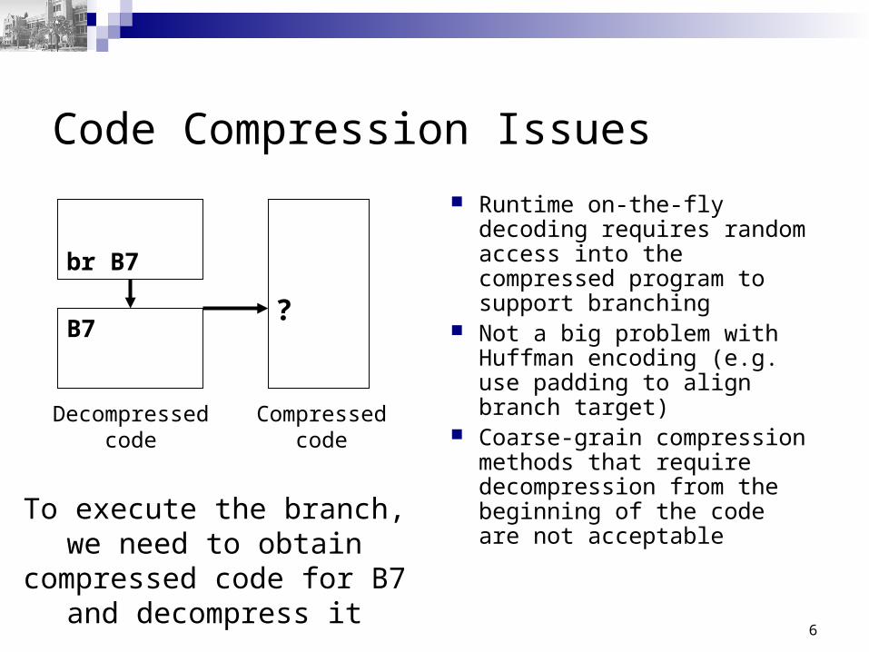
Runtime on-the-fly decoding requires random access into the compressed program to support branching

Not a big problem with Huffman encoding (e.g. use padding to align branch target)

Coarse-grain compression methods that require decompression from the beginning of the code are not acceptable

br B7

B7?

Decompressedcode

Compressedcode

To execute the branch,we need to obtain

compressed code for B7and decompress it

7

Compression Options

Code compression can take place in three different places:

1. Instructions can be decompressed on fetch from cache2. Instructions can be decompressed when refilling the

cache from memory3. Program can be decompressed when loaded into

memory

8

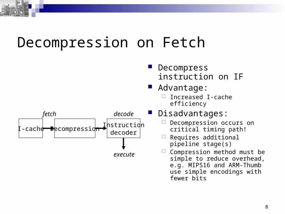
Decompression on Fetch

Decompress instruction on IF Advantage:

Increased I-cache efficiency

Disadvantages: Decompression occurs on

critical timing path! Requires additional pipeline

stage(s) Compression method must be

simple to reduce overhead, e.g. MIPS16 and ARM-Thumb use simple encodings with fewer bits

Instructiondecoder

DecompressionI-cache

fetch decode

execute

9

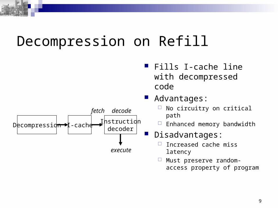
Decompression on Refill

Fills I-cache line with decompressed code

Advantages: No circuitry on critical path Enhanced memory bandwidth

Disadvantages: Increased cache miss latency Must preserve random-access

property of program

Instructiondecoder

Decompression I-cache

fetch decode

execute

10

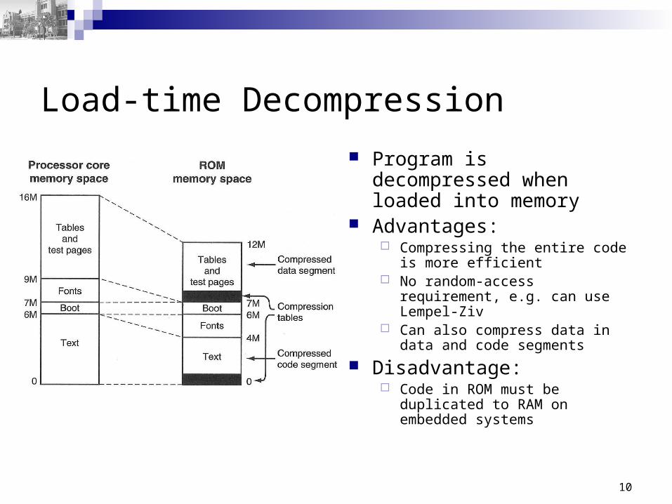
Load-time Decompression

Program is decompressed when loaded into memory

Advantages: Compressing the entire code

is more efficient No random-access

requirement, e.g. can use Lempel-Ziv

Can also compress data in data and code segments

Disadvantage: Code in ROM must be

duplicated to RAM on embedded systems

11

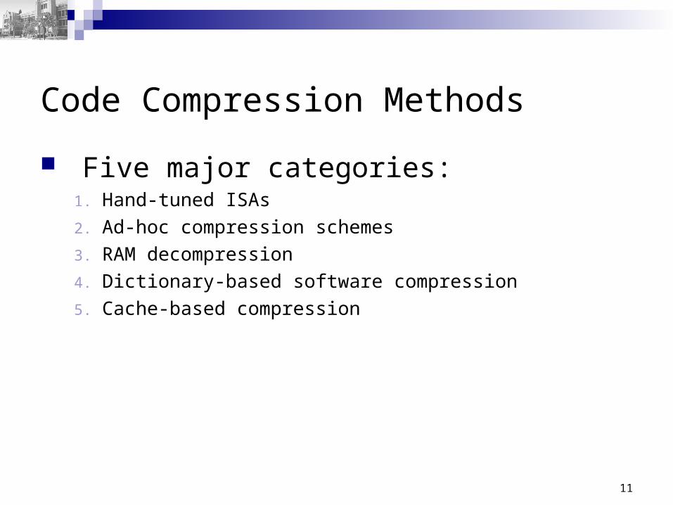
Code Compression Methods

Five major categories:1. Hand-tuned ISAs2. Ad-hoc compression schemes3. RAM decompression4. Dictionary-based software compression5. Cache-based compression

12

Hand-tuned ISAs

Most commonly used in CISC and DSP world Reduce instruction size by designing a compact

ISA based on operation frequencies Disadvantages:

Makes the ISA more complex and the decode stage more expensive

Makes the ISA non-orthogonal hampering compiler optimizations and inflexible for future extensions of the ISA

13

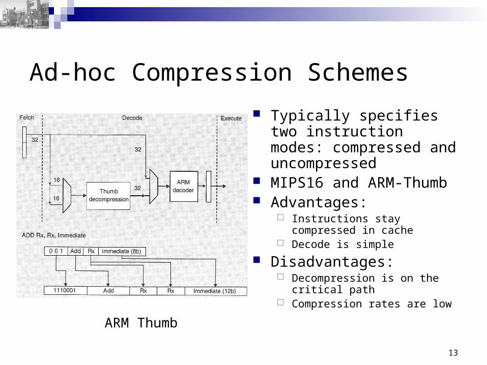
Ad-hoc Compression Schemes

Typically specifies two instruction modes: compressed and uncompressed

MIPS16 and ARM-Thumb Advantages:

Instructions stay compressed in cache

Decode is simple

Disadvantages: Decompression is on the

critical path Compression rates are low

ARM Thumb

14

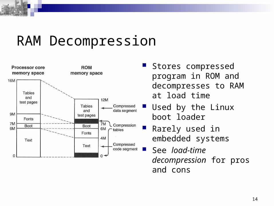
RAM Decompression

Stores compressed program in ROM and decompresses to RAM at load time

Used by the Linux boot loader Rarely used in embedded

systems See load-time decompression

for pros and cons

15

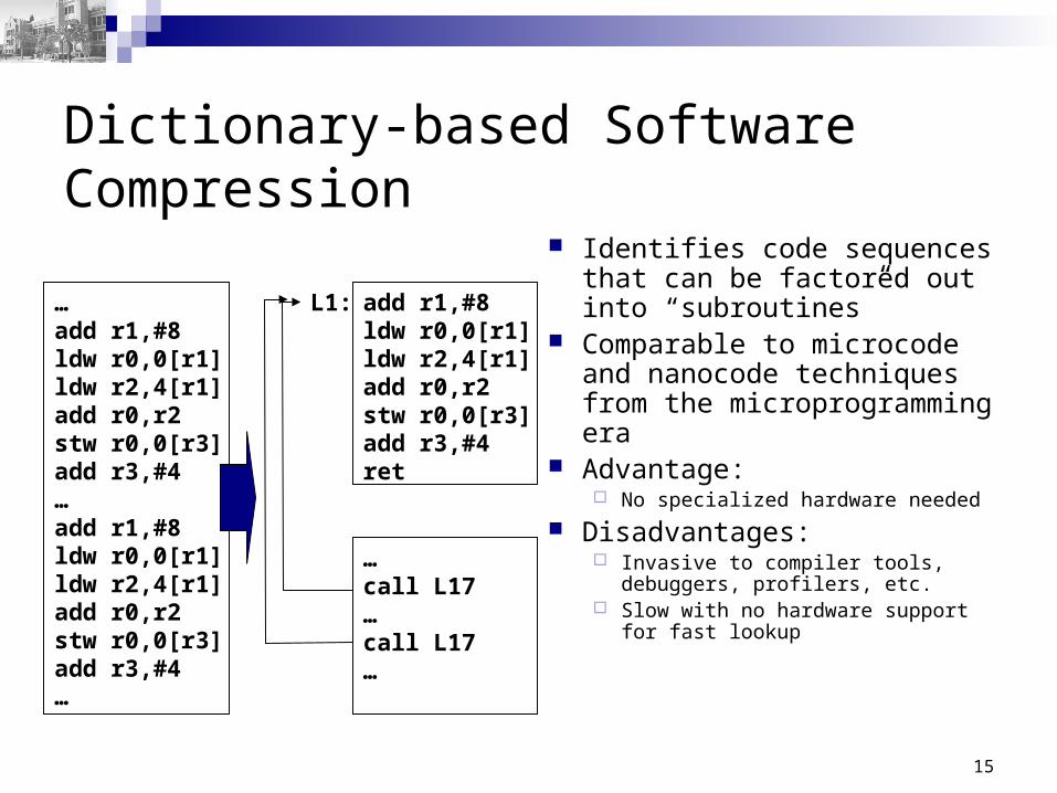
Dictionary-based Software Compression

Identifies code sequences that can be factored out into “subroutines”

Comparable to microcode and nanocode techniques from the microprogramming era

Advantage: No specialized hardware

needed

Disadvantages: Invasive to compiler tools,

debuggers, profilers, etc. Slow with no hardware support

for fast lookup

add r1,#8ldw r0,0[r1]ldw r2,4[r1]add r0,r2stw r0,0[r3]add r3,#4ret

…add r1,#8ldw r0,0[r1]ldw r2,4[r1]add r0,r2stw r0,0[r3]add r3,#4…add r1,#8ldw r0,0[r1]ldw r2,4[r1]add r0,r2stw r0,0[r3]add r3,#4…

…call L17…call L17…

L1:

16

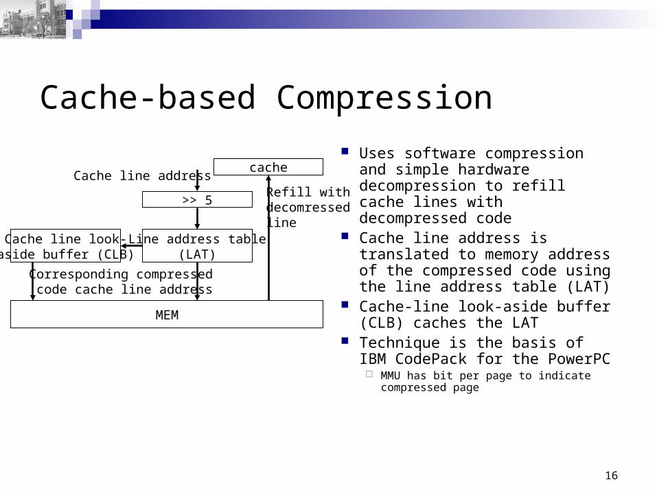
Cache-based Compression

Uses software compression and simple hardware decompression to refill cache lines with decompressed code

Cache line address is translated to memory address of the compressed code using the line address table (LAT)

Cache-line look-aside buffer (CLB) caches the LAT

Technique is the basis of IBM CodePack for the PowerPC MMU has bit per page to indicate

compressed page

Cache line address

>> 5

Line address table(LAT)

Corresponding compressedcode cache line address

MEM

Cache line look-aside buffer (CLB)

Refill withdecomressedline

cache

17

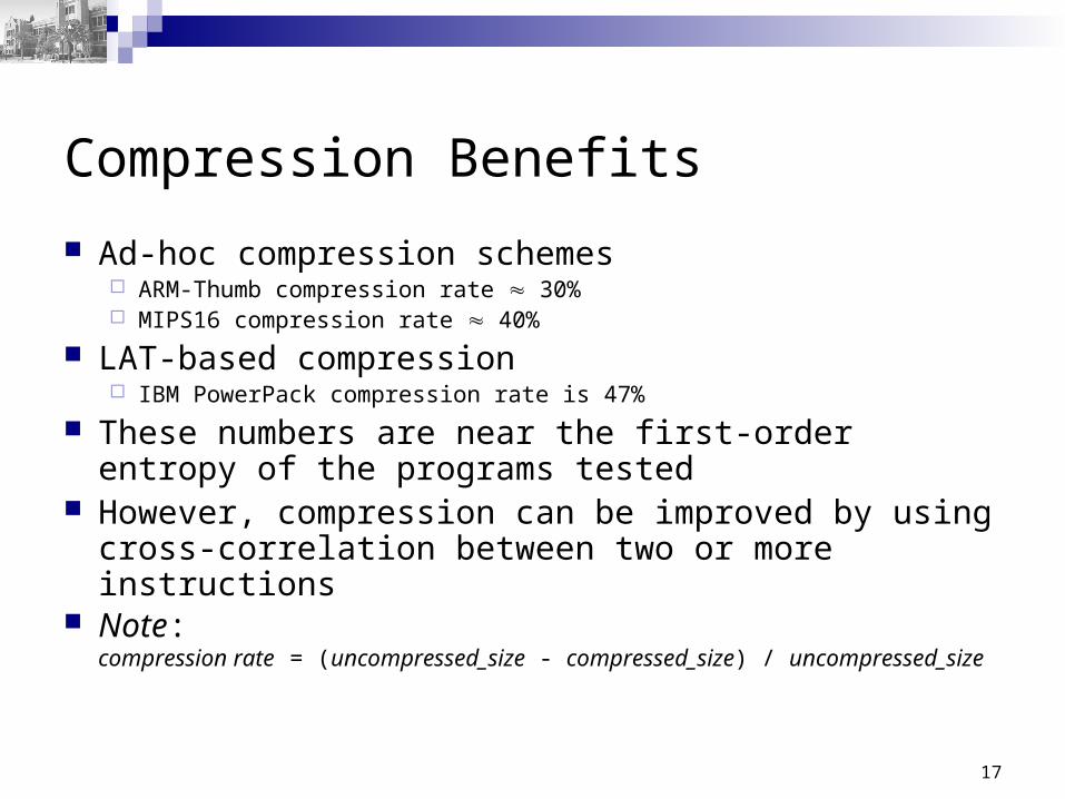
Compression Benefits

Ad-hoc compression schemes ARM-Thumb compression rate 30% MIPS16 compression rate 40%

LAT-based compression IBM PowerPack compression rate is 47%

These numbers are near the first-order entropy of the programs tested

However, compression can be improved by using cross-correlation between two or more instructions

Note:compression rate = (uncompressed_size - compressed_size) / uncompressed_size