Code Compression in Embedded Systems -...

Code Compression in Embedded Systems

by

ID

Date: March 22, 2002


_____________________________________________________________________________________________

____________________________________________________________________________________________ of 39

IntroductionEmbedded systems are becoming increasingly popular as more and more consumers accept the carrying electronic

devices with them. For many people, handheld devices such as cellular phones, pagers, digital cameras, PalmPilots,

and PocketPC’s have become like wristwatches; the owner simply would not go anywhere without them. It is no

surprise that some people feel as if embedded systems will become the next major computer science research field

that will follow the current boom of interest in networks, and past interest in parallel processing.

Problem StatementEmbedded devices’ popularity conceals the constraints that designers face when developing for these systems .

Embedded systems that drive handheld devices are designed to be small so as to be comfortable to hold and carry.

These systems are targeted toward large volume sales, hence they are cost-sensitive. Cost is strongly associated

with size of the integrated circuits (ICs) used in a device [LiDK 1999]. Much of an embedded system’s IC space is

devoted to memory for program code and data [LiDK 1999]. Many embedded systems are further limited by the

need to operate off a limited power source, usually batteries, hence power consumption is a major concern when

designing their components. Larger storage, memory, and cache sizes, and faster CPUs all contribute to space, cost,

and power use. Because of these factors, memory and storage space both are limited in handheld devices, affecting

designers, developers and users.

RISC has become the dominant CPU design paradigm, replacing CISC. Storing CPU control signals within the

instruction, finely tuning pipelines, and fixing instruction lengths have all contributed to the performance of RISC

architectures. RISC does however increase instruction size, increasing demand for memory.

Use of High Level Languages (HLL) lowers development and maintenance cost and time. Statistics on

programming language use gathered by Dataquest show use of HLLs replacing assembly language in embedded

systems [LiDK 1999]. Handheld systems are more prone to use HLLs. The drawback of these languages is the

increased code size. Code size increases both due to code bloat and due to compilers that have traditionally been

optimized for speed, not size. As the gap between CPU and memory speed widens, the amount of slowing due to

cache misses is further enlarged.

A solution to many of these constraints is code compression. Compression can be used to reduce the size of

programs in storage and memory. In so doing, it can reduce the size of components needed, lowering power

requirements, size, and cost.

Benefits of Code CompressionCode compression has many benefits. The reduced program size can be used to reduce the size of storage necessary

on IC’s. This can save production costs. Since memory consumes a significant amount of an embedded system’s

power and power consumption is proportional to IC area, battery life can be extended [YSOO 1997]. Smaller chips

also have lower capacitance, which lowers power consumption [LeHW 2000:2].


_____________________________________________________________________________________________

____________________________________________________________________________________________ of 39

When a cache miss occurs, the data brought to the instruction cache (I-cache) is loaded from main memory

compressed, so less data needs to be transmitted on the bus between memory and I-cache. If the code is compressed

in the I-cache, then less data is sent out from the I-cache with each instruction fetch. Thus, fewer bit toggles are

necessary on bus lines, which reduces power consumption [ViZA 2000]. Furthermore, if code in the I-cache is

uncompressed, then less data is transmitted on the bus from memory to the I-cache, so the cache may be filled

sooner. If code in the I-cache is compressed, then it is able to hold many more instructions, reducing the cache miss

rate. Both of these cases cause the CPU to pause for less time due to cache misses. Since the CPU is the main

consumer of power, compression can result in significant power savings [ViZA 2000, LeHW 2000:3]. If memory

and or cache are made smaller, their effective capacitance decreases further decreasing power consumption [LeHW

2000:2]. Because there are fewer transactions and transactions are shorter, compression may also increase

performance (reduce program execution time).

Introduction to Data CompressionCompression schemes try to reduce the number of bits required to represent data. In the following section, key

concepts of data compression and common data compression techniques will be introduced.

Measuring CompressionOne way to measure of compression is the amount by which data was reduced in size, expressed as a percentage.

For example, consider a 49,402,412 byte sound clip that is compressed to a 4,481,024 byte MP3 file. The reduction

in size is 1 - 4,481,024 / 49,402,412 = 9.07%.

A more common measure of compression is the compression ratio, which is defined as the ratio of the compressed

data to the original data. It may be expressed as a decimal number or as a percentage. In our example, the

compression ratio is 4,481,024 / 49,402,412 = .0907 or 9.07 %. Such a compression ratio is not uncommon for MP3

files.

EntropySuppose a random experiment is taking place. Let P(A) be the probability that some event A will occur. The

information content of A is denoted i(A) and defined as:

i(A) = - logb P(A)

Suppose that the set of independent events Ai represent the set of all possible outcomes of a random experiment. Let

P(Ai) be the probability that event A i occurs for each A i. The average information associated with the experiment is:

∑ ∑−== )(log)()()( ibiii APAPAiAPH

This quantity is called entropy. Claude Shannon showed for b = 2, entropy was the average number number of bits

needed to encode the output of a source. He further showed that encoding the output of a source with an average

number of bits equal to the entropy of the source is the best any compression scheme can achieve. As a


_____________________________________________________________________________________________

____________________________________________________________________________________________ of 39

consequence, known compression schemes attempt to compress files to sizes close to the entropy, but cannot

compress programs smaller than it.

Codeword ClassificationCodes can be further classified as fixed, static, or adaptive based on the type of codewords , that is output words,

that they generate. In fixed codes, for all input streams, each input symbol corresponds to the same codeword. In

static codes, the relationship between input symbols and codewords is selected by a model that matches a particular

input stream, but does not change during the processing of that stream. Additional information such as the model or

a dictionary must be transmitted with the encoding in order for the decoder to recover the original sequence.

Adaptive codes feature codewords that change while a given input stream is processed; selection and modification

of codewords is dictated by a model.

Dictionary MethodsDictionary methods for performing compression create a table of frequently occurring symbols or sequences of

symbols. When the encoder encounters a symbol or sequence that is in its dictionary, it will place a special escape

character on the output followed by the index into the dictionary of that symbol. Regular symbols are simply

encoded as themselves. In applications where the table is large and has a high probability of containing an encoding

for each symbol, this schema can also be reversed with escape characters only used before an input symbol is

written directly to output.

Construction of the dictionary can be done by hand, or by heuristic methods, especially those that examine the

typical source data stream. Fixed codes will have the same table for all sources, static codes will provide a new

table for each source, and adaptive codes will create the table while processing the source. Dictionary methods

using static codes are common to compression of program code; the table is created by encoder during compression

and is saved with the compressed output.

Markov ModelsWhen information is available about the data sets that are to be compressed, models can be constructed that allow

more efficient compression algorithms. The simplest model is to assign probabilities to each letter of the alphabet.

Markov Models, named after mathematician Andrei Markov, combine the history of elements with probabilities. A

kth-order Markov model uses the history of the last k elements to appear on the input stream to predict the next

symbol. Markov Models are often used in fixed codes.

Each possible history is associated with a state. Thus each state has m transitions (one for each possible next input

symbol). In total, there are with km possible states. Each transition from a state has a probability associated with it;

because the state is reached by the last k transitions taken, that probability is based upon the last k elements encoded.

As a simple example, consider the English language. If we knew that the last encoded character was the letter q,

there would be a high probability that the next character is u.


_____________________________________________________________________________________________

____________________________________________________________________________________________ of 39

Static Huffman CodesHuffman coding is a bottom up method for organizing elements into a tree. The shape of the built tree determines

the codeword for each element.

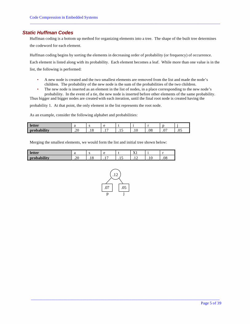
Huffman coding begins by sorting the elements in decreasing order of probability (or frequency) of occurrence.

Each element is listed along with its probability. Each element becomes a leaf. While more than one value is in the

list, the following is performed:

• A new node is created and the two smallest elements are removed from the list and made the node’schildren. The probability of the new node is the sum of the probabilities of the two children.

• The new node is inserted as an element in the list of nodes, in a place corresponding to the new node’sprobability. In the event of a tie, the new node is inserted before other elements of the same probability.

Thus bigger and bigger nodes are created with each iteration, until the final root node is created having the

probability 1. At that point, the only element in the list represents the root node.

As an example, consider the following alphabet and probabilities:

letter a s e t i r p jprobability .20 .18 .17 .15 .10 .08 .07 .05

Merging the smallest elements, we would form the list and initial tree shown below:

letter a s e t X1 i rprobability .20 .18 .17 .15 .12 .10 .08

.12

.07 .05p j


_____________________________________________________________________________________________

____________________________________________________________________________________________ of 39

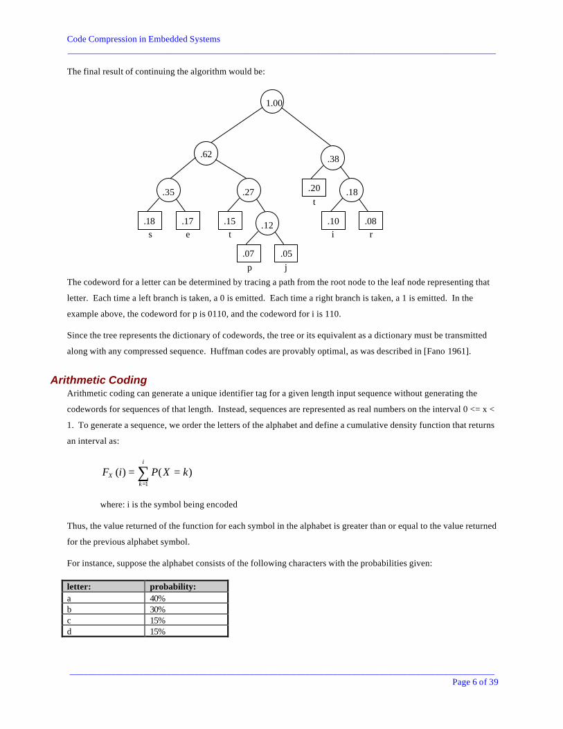
The final result of continuing the algorithm would be:

The codeword for a letter can be determined by tracing a path from the root node to the leaf node representing that

letter. Each time a left branch is taken, a 0 is emitted. Each time a right branch is taken, a 1 is emitted. In the

example above, the codeword for p is 0110, and the codeword for i is 110.

Since the tree represents the dictionary of codewords, the tree or its equivalent as a dictionary must be transmitted

along with any compressed sequence. Huffman codes are provably optimal, as was described in [Fano 1961].

Arithmetic CodingArithmetic coding can generate a unique identifier tag for a given length input sequence without generating the

codewords for sequences of that length. Instead, sequences are represented as real numbers on the interval 0 <= x <

1. To generate a sequence, we order the letters of the alphabet and define a cumulative density function that returns

an interval as:

∑=

==i

kX kXPiF

1

)()(

where: i is the symbol being encoded

Thus, the value returned of the function for each symbol in the alphabet is greater than or equal to the value returned

for the previous alphabet symbol.

For instance, suppose the alphabet consists of the following characters with the probabilities given:

letter: probability:a 40%b 30%c 15%d 15%

.12

.07 .05p j

.27

.15t

.35

.18 .17s e

.62

.18

.10 .08i r

.38

.20t

1.00


_____________________________________________________________________________________________

____________________________________________________________________________________________ of 39

We could let the cumulative density function for each character be represented as:

letter i: FX(i):a 0.40b 0.70c 0.85d 1.00

Arithmetic coding algorithms generally work in the following manner. The interval under consideration begins as

[0.0, 1.0). Let [lj, hj) represent the current lower and higher bound of the interval. For each letter xn on the input that

is read, and the corresponding range FX(xn) for that letter is found. The interval is shrunk to [li+1, hi+1 ) where:

li+1 = li + (hi - li) * FX(xn-1)hi+1 = li + (h i - li) * FX(xn )

Algorithms either terminate by sending both the lower and higher bounds of the interval corresponding to the

sequence to be encoded, or by sending any value within the interval (but preceding transmission by the number of

characters to be encoded).

As an example, consider the sequence “bcac”. The interval begins as [0.00, 1.00). FX(a) is 0.40, FX(b) is 0.70.

Encoding the letter b results in the range [0.00 + (1.00 - 0.00) * 0.40, 1.00 + (1.00 - 0.00) * 0.70) = [0.40, 0.70).

Encoding the letter c results in the range [0.40 + (0.70-0.40) * 0.70, 0.40 + (0.70-0.40) * 0.85) = [0.61, 0.655).

Encoding the letter a results in the interval [0.61, 0.628). Encoding the last letter c results in the interval [0.6226,

0.6253). The encoder can either transmit this range or can transmit that the number of characters encoded is 4

followed by any value from this range.

An additional useful fact about arithmetic coding is that the average codelength lA for a string of length m is bound

by:

mXHlXH A

2)()( +≤≤

Therefore, arithmetic compression is nearly optimal for any distribution. The drawback is that coding delay can be

very long.

Lempel-Ziv 78In Lempel-Ziv 78 (LZ78), a table is built as the encoder processes the input stream using a greedy matching scheme.

The algorithm operates as follows. The longest prefix of the input stream that exists in the dictionary is found.

Label this prefix as P. If no such prefix exists, P is set to null. Let p be the index of P in the dictionary. If there is

no matching prefix in the dictionary, p is set to a special value ø. The input character that follows P is c. Now c is

read. The output (p, c) is transmitted. Then the string P•c is added to the dictionary, where • represents

concatenation.


_____________________________________________________________________________________________

____________________________________________________________________________________________ of 39

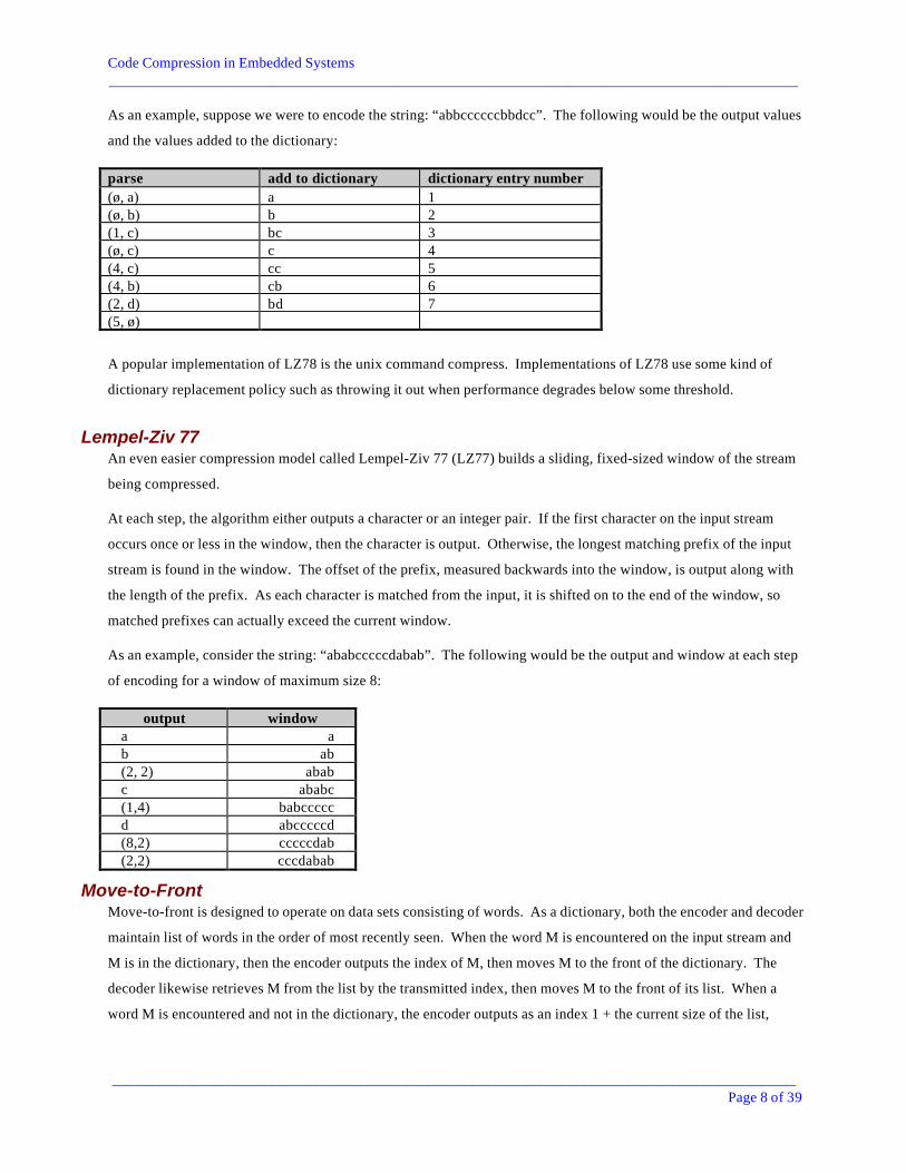
As an example, suppose we were to encode the string: “abbccccccbbdcc”. The following would be the output values

and the values added to the dictionary:

parse add to dictionary dictionary entry number(ø, a) a 1(ø, b) b 2(1, c) bc 3(ø, c) c 4(4, c) cc 5(4, b) cb 6(2, d) bd 7(5, ø)

A popular implementation of LZ78 is the unix command compress. Implementations of LZ78 use some kind of

dictionary replacement policy such as throwing it out when performance degrades below some threshold.

Lempel-Ziv 77An even easier compression model called Lempel-Ziv 77 (LZ77) builds a sliding, fixed-sized window of the stream

being compressed.

At each step, the algorithm either outputs a character or an integer pair. If the first character on the input stream

occurs once or less in the window, then the character is output. Otherwise, the longest matching prefix of the input

stream is found in the window. The offset of the prefix, measured backwards into the window, is output along with

the length of the prefix. As each character is matched from the input, it is shifted on to the end of the window, so

matched prefixes can actually exceed the current window.

As an example, consider the string: “ababcccccdabab”. The following would be the output and window at each step

of encoding for a window of maximum size 8:

output windowa ab ab(2, 2) ababc ababc(1,4) babcccccd abcccccd(8,2) cccccdab(2,2) cccdabab

Move-to-FrontMove-to-front is designed to operate on data sets consisting of words. As a dictionary, both the encoder and decoder

maintain list of words in the order of most recently seen. When the word M is encountered on the input stream and

M is in the dictionary, then the encoder outputs the index of M, then moves M to the front of the dictionary. The

decoder likewise retrieves M from the list by the transmitted index, then moves M to the front of its list. When a

word M is encountered and not in the dictionary, the encoder outputs as an index 1 + the current size of the list,

Code Compression in Embedded Systems Miller_____________________________________________________________________________________________

____________________________________________________________________________________________ of 39

followed by M. The decoder receiving an index beyond the end of the list knows to receive the word M. Both

encoder and decoder finish by placing the word M at the front of the list.

As an example, consider the string “the first man went in first before the man first in line”. The following is a table

showing the word being considered, the encoder’s output, and the list after the output is sent.

current word output list after outputthe 1, the thefirst 2, first first theman 3, man man first thewent 4, went went man first thein 5, in in went man first thefirst 4 first in went man thebefore 6, before before first in went man thethe 6 the before first in went manman 6 man the before first in wentfirst 4 first man the before in wentin 5 in first man the before wentline 7 line in first man the before went

Special Requirements of Code Compression SystemsIn order to be useful, the compression system itself must be small. This implies a simple compression algorithm so

as to use little processor time and take up little memory (or to use less power and fit on a smaller IC for hardware

compression). The system must run all existing programs correctly.

Control transfer instructions present a problem for compression systems. The target of a branch instruction in

uncompressed code will change when the code is compressed. Programs also frequently contain relative or

computed branch targets. Researchers have developed several solutions.

Most existing compression systems such as the Lempel-Ziv algorithms used by compress, gzip, and pkzip use a

beginning to end, variable length encoding. Thus, they require the entire program be decompressed from beginning

to end before it can be used. Because these compression schemes would not reduce memory use, researchers have

developed special compression systems capable of decompressing a blocks or instructions of a program

independently, allowing random access to the program.

Classifications of Code Compression SystemsA survey of code compression systems must organize them by some means of classification. Several criteria are

described in this section.

An obvious classification criterion is the method of compression used. Many systems use some sort of dictionary

building technique. Many of these dictionary techniques operate by preprocessing the source code or executable

while scanning for frequent patterns, then filling dictionaries using heuristic selection criteria. Several specifically

use Huffman coding to build dictionaries. Others use fixed Markov models, arithmetic coding, or even original and

specialized tree building methods. This paper organizes code compression systems by the method of compression.


____________________________________________________________________________________________ of 39

Classification may also be done based on the location where decompression takes place. As was mentioned above,

complete decompression of the program as it is loaded into memory is not practical for embedded systems.

Decompression might take place as the compressed code is loaded into the instruction cache, in the instruction

cache, or between the instruction cache and the CPU.

Most researchers tested their compression ideas in real systems. As Wolfe and Chanin pointed out, running their

compression systems “on actual ebmedded (sic) applications would have been preferable, accurate execution traces

from these types of programs were not available” [WoCh 1992]. Many researchers ran their compression systems

on benchmarks, such as I-Cheng Chen et al or Jin and Chen who used SPEC95 [ChBM 1997, JiCh 2000]. Some

created their own benchmarks, suggesting that popular programs were important to test, as was done by Liao who

compressed programs like compress, gzip, and jpeg [LiDK 1999]. Creation of benchmarks was especially common

for researchers limited to domains where common benchmarks didn’t exist, like the small memory Java domain

studied by Clausen et al who compressed standard Java libraries [CPCM 2000]. Benchmarks were also created

when certain programs were found to demonstrate noteworthy effects [LeHW 2000:3]. A few only simulated

execution on hardware design tools, which may lead to questionable results, although simulation was often done out

of necessity, since the researchers were focused on non-measurable quantities like energy usage of each component

of the system [CoMc 1999].

Compression schemes differ in the size of symbols being compressed. Early compression systems worked on each

byte, as do the unix commands compress and gzip [WoCh 1992]. Later on, it became common to use full

instructions as symbols such as in [YSOO 1997, LeHW 2000:3]. Dictionary building techniques such as [ChBM

1997] and [LBCM 1997] operated on sequences of instructions within basic blocks; some such as [LiDK 1999] even

operated on symbols spanning basic blocks. The unique Slim Binaries compression scheme compressed abstract

syntax tree branches [FrKi 1997]. The late 1990’s saw a concept for RISC systems where various instructions have

similar boundaries at which operands, immediate constants, or store addresses start. Instructions themselves were

split up into groups of bits called streams, with bits from each instruction in group 1 being compressed separately

from those from group 2 and so on [JiCh 2000]. [KoWo 1994] even compared several symbol sizes.

When code is compressed, the intended destination addresses of branches change. Because instructions are

condensed, relative branches may overshoot their target, and direct branches may point past the end of the program.

The first attempt to overcome the branch problem was to build a table translating addresses of blocks in

uncompressed code to addresses in compressed code, with the stipulation that all instructions in the block may have

to be decompressed to reach the exact target instruction [WoCh 1992]. Researchers using fixed sized codewords

were able to use similar translation tables without the need to decompress the entire block to reach the target [JiCh

2000]. Later researchers frequently patched branches whenever possible (although patching relative branches is

known to be NP complete) and modified the hardware of the system to accept branches the size of the smallest

codewords [LBCM 1997, Larin 1999]. Some researchers patched branches, but did not change rest of the systems,

thus requiring branch targets to be padded for word alignment [BeMN 1999]. Other researchers even performed

modifications on branches and used them as part of the compression scheme [CoMc 1999].


____________________________________________________________________________________________ of 39

Machine Instruction MethodsOne of the simplest methods for shrinking the size of code is to shrink the size of instructions. Two commercial

proposals for such methods are ARM Thumb and MIPS16, both of which feature 16-bit instructions based on a 32-

bit instruction set. The shortened instructions supplement use of 32-bit instructions on the processor core, while

requiring support from the core [BeMN 2001]. In each system, the processor core expands the 16-bit instruction to

32 bits just after they are fetched from instruction memory [LBCM 1997]. Instructions chosen for the Thumb set

were selected due to their frequency of use, importance for generating small code, or lack of need for full 32 bits.

Instructions for the MIPS16 set were chosen by analyzing a number of applications to determine the most frequently

generated instructions [LBCM 1997]. In order to reduce the number of instruction bits to 16, the number of registers

that can be referenced was decreased to 8, and the size of immediate fields was shrunk [LBCM 1997]. Neither

shortened instruction set is capable of generating complete programs; special instructions are used to switch between

16-bit and 32-bit instruction modes [LBCM 1997].

Use of the supplemental shortened instructions does decrease code size. ARM programs compiled with Thumb

support have code sizes about 30% less than when compiled for 32-bit instructions alone [LBCM 1997]. Similarly,

code sizes in programs produced with MIPS16 support are about 40% smaller than for programs using only 32-bit

MIPS-III instructions [LBCM 1997].

Huffman Coding MethodsHuffman coding methods were used to assign variable length codewords to frequently occurring bytes or parts of

instructions. Since codewords were variable length, a translation table was always needed to map uncompressed

branch addresses to compressed ones. For maximum decoding speed, the Huffman codes were made fixed and

decoders were implemented using PLAs in hardware. As for all methods, results are summarized in a table in the

conclusion.

Wolfe and ChaninIn the paper that started interest in code compression for embedded systems, Wolfe and Chanin proposed their

method of compressing RISC instructions in what was called CCRP, “Code Compressed RISC Processor” [WoCh

1992]1. Each cache line was compressed, and code was expanded by the cache refill engine as code was loaded into

the cache so as to avoid problems when branch targets change due to compression. The mapping created by the

compressor for translating branch addresses was called a Line Address Table, or LAT, and only mapped to the start

of blocks. Therefore, several instructions may have to be decompressed from the block before the target instruction

was finally found. The most recently used LAT entries stored in the special cache called the Cached Lookaside

Buffer, or CLB. Each LAT entry had a 24 bit base address followed by 8 entries indicating the length of the next

compressed block. The LAT added 3.125% to the size of programs.

Compression was done on bytes, with more frequent bytes being assigned shorter variable-length codewords. Wolfe

and Chanin ran experiments to determine if having a fixed code system would degrade compression ratios compared


____________________________________________________________________________________________ of 39

to having a static code system, and found little difference between the two. The researchers selected the fixed route

because it allowed the decompressor to be effectively hardwired using a PLA, for maximum speed. Instruction

bytes are encoded using a bounded Huffman technique in which codewords are selected to be from 1 bit long to not

more than 16 bits (the upper bound).

Wolfe and Chanin tested performance using the MIPS2000 architecture on C and FORTRAN programs.

Compression ratios ranged from 65% to 75%. Three different memory models were tried: EPROM, Burst EPROM,

and Static Column DRAM. The latter two models had the advantage that each subsequent word after the first word

only took one clock cycle to retrieve. For the latter two, the performance of the system using compression was even

greater than that of the original system.

Tests of different cache sizes found that increasing sizes from 256 bytes to 512 made a difference, but increases

beyond 1024 bytes had lessening effect. The size of the CLB was not a signficant bottleneck on performance. One

of the most important tests correlated memory speed to miss rate. It was found that for high miss rates, if memory

was slow, then compression improved performance; alternately, if memory was relatively fast, than compression

reduced performance.

A follow up study by Kozuch and Wolfe compared compression for 15 programs from the SPEC benchmark suite

the VAX 11, MIPS R4000, SUN 68020, SPARC, IBM RS6000, and Motolora MPC603 architectures [KoWo 1994].

It was found that statically compiled programs varied in size considerably, from MIPS programs being about 2.7

times the size of those for a VAX, to MPC603 programs being almost 4.9 times as large. Executable size variance

was due to architecture, compiler trade-offs, and library sizes [KoWo 1994]. In order to determine whether less

dense code was more compressible, the zeroth and first order entropy of the programs on each architecture was

calculated. Due to their importance, results for code size and entropy are shown in Figure 1 and Figure 2 below:

Figure 1: Program Sizes for EachArchitecture [KoWo 1994].

Figure 2: Average Entropy for EachArchitecture [KoWo 1994].

The results demonstrate that the MIPS instruction set is much more compressible than other instruction sets using

zeroth-order compression, which can explain variation in results found by other researchers who tried similar

compression methods. Furthermore, first order can achieve substantial compression improvement, but higher order

techniques (like gzip uses) are worth searching for regardless of the fact that most they are often too expensive to

1 Information in this section is drawn from [WoCh 1992] unless otherwise noted.


____________________________________________________________________________________________ of 39

implement for run-time decompression on embedded systems. Returning to their own work, CCRP, Kozuch and

Wolfe found that the ratio of zeroth-order entropy to their compression ratio was 94 to 95%, indicating that they

were achieving good rates even though their method required the overhead of a LAT [KoWo 1994].

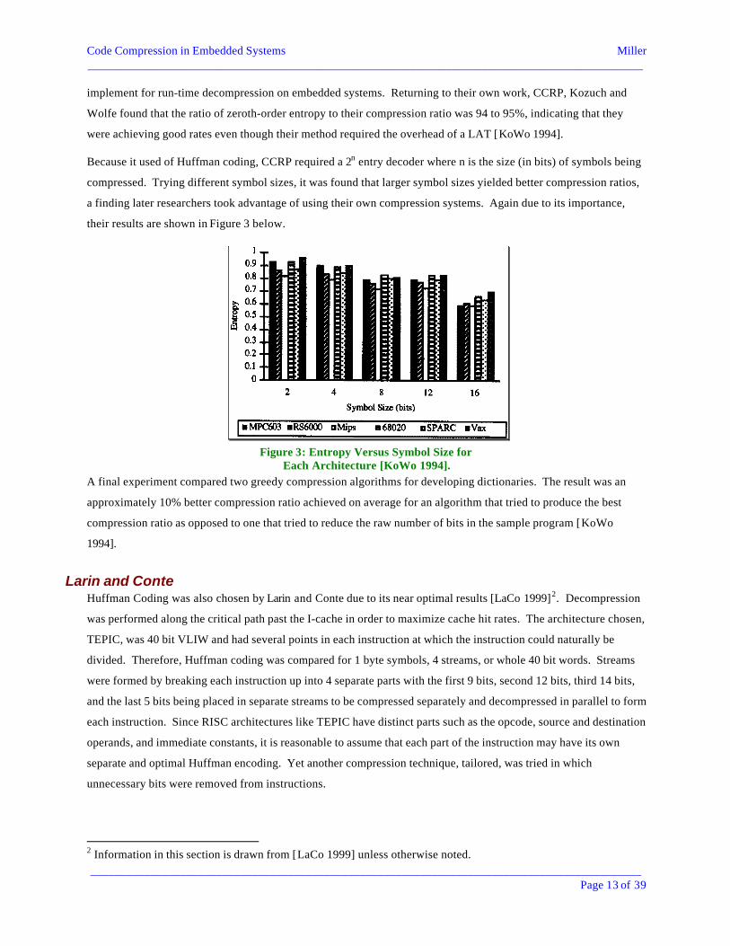
Because it used of Huffman coding, CCRP required a 2n entry decoder where n is the size (in bits) of symbols being

compressed. Trying different symbol sizes, it was found that larger symbol sizes yielded better compression ratios,

a finding later researchers took advantage of using their own compression systems. Again due to its importance,

their results are shown in Figure 3 below.

Figure 3: Entropy Versus Symbol Size forEach Architecture [KoWo 1994].

A final experiment compared two greedy compression algorithms for developing dictionaries. The result was an

approximately 10% better compression ratio achieved on average for an algorithm that tried to produce the best

compression ratio as opposed to one that tried to reduce the raw number of bits in the sample program [KoWo

1994].

Larin and ConteHuffman Coding was also chosen by Larin and Conte due to its near optimal results [LaCo 1999]2. Decompression

was performed along the critical path past the I-cache in order to maximize cache hit rates. The architecture chosen,

TEPIC, was 40 bit VLIW and had several points in each instruction at which the instruction could naturally be

divided. Therefore, Huffman coding was compared for 1 byte symbols, 4 streams, or whole 40 bit words. Streams

were formed by breaking each instruction up into 4 separate parts with the first 9 bits, second 12 bits, third 14 bits,

and the last 5 bits being placed in separate streams to be compressed separately and decompressed in parallel to form

each instruction. Since RISC architectures like TEPIC have distinct parts such as the opcode, source and destination

operands, and immediate constants, it is reasonable to assume that each part of the instruction may have its own

separate and optimal Huffman encoding. Yet another compression technique, tailored, was tried in which

unnecessary bits were removed from instructions.

2 Information in this section is drawn from [LaCo 1999] unless otherwise noted.


____________________________________________________________________________________________ of 39

Larin and Conte’s branch translation table held mappings to exact locations for each unique branch. Due to its finer

granularity, the table added on average 15.5% to the size of the program. It also cached entries near the CPU.

The cache also stored the predicted PC following an instruction in order to help keep the CPU pipeline moving at

full speed, and stored a branch taken/not taken predictor value. Operations were collected into word aligned groups,

with an extra bit somewhat wastefully following each instruction and being set only for the last instruction in the

group.

Code compression ratios of stream and byte encodings produced little difference for this architecture, hovering

around 70% to 78%. Tailored encoding did better ranging from 60% to 67%. Finally, full instruction compression

was at least twice as good in all cases, typically achieving ratios of 23% to 30%. One should note that the

compression rate of full Huffman encoding is offset by the enormous table required to decode it.

Decoder complexity in terms of decoder size was also measured. Complexity for Huffman compression of full

instructions was normally several times that for stream compression, and both were about 100 times more complex

than for byte compression. The poor performance of stream compression was not explained by the authors. Bus

flips are the main cause of power consumption across the bus. On average, the number of flips for base compression

was several times larger than that for tailored compression, which was itself several times for that of Huffman

compression.

Single Instruction Dictionary MethodsEach of the methods in this section operates using some form of dictionary building. Typically, the most frequent

instructions are stored in a dictionary. In the code, a tag and an index into the dictionary replace the instruction.

There is strong evidence that this will work. Just as Hennessy and Patterson found in 1990 that 90% of program

execution time is spent in 10% of the code, Lefurgy obsevered:

On average, less than 20% of the instructions... have bit pattern encodings which are used exactly

once in the program. In the go benchmark, for example, 1% of the most frequent instruction

words account for 30% of the program size, and 10% of the most frequent instruction words

account for 66% of the program size.

[HePa 1990, LBCM 1997]

Even shortening the 1% most frequent instructions in a program from 32 bits to 8 bits would reduce the code size by

22.5%.

Yoshida, Song, Okuhata, Onoye, and ShirakawaYoshida et al [YSOO 1997]3 noted that compilers tend to generate many duplicate instructions. They developed a

compression algorithm with the goal of reducing power consumption. Their algorithm operates by searching

through the program of N instructions, each having m bits, to find a complete list of n distinct instructions. Since

programs only use part of the instruction set and compilers generate many duplicate instructions, this is not difficult.

3 Information in this section is drawn from [YSOO 1997] unless otherwise noted.


____________________________________________________________________________________________ of 39

Then, a log2 n bit number is assigned to each instruction. A table is created to transform each code number to a full

instruction. This reduces the size of instructions from m bits to log2 n bits. An optional subcode compression

extension was to further reduce the size of instructions by separately compressing codes for registers and flags.

Power dissipation of memory units depends on their physical size. Power use reduction was quantified by the

equation:

Nm

knmnNPf

+−=

log1/ο

where k is the power dissipation ratio of the on-chip memory.

Using the ARM610 processor core, Yoshida et al ran their compression system on the dhrystone benchmark.

Opcode size of compressed programs typically decreased from 32 bits to 12 bits for a program compression ratio of

22.7% to 54.0% (or 4.48% to 21.52% with 3 bit subcode compression), and a power reduction of memory by

19.57% to 42.33% (16.46% to 24.55% with 3 bit subcode compression). In [YSOO 1996], it was found that placing

the decompression software in ROM required only 1.67 mm2 area using 0.6 µm technology. Battery life was

estimated to have been extended by 1.7 times [YSOO 1996].

Jin and ChenJin and Chen [JiCh 2000]4 realized that the capability of code compression could be enhanced if decompression was

done past the cache. To perform compression, each 64-bit instruction is broken up into 4 sections of 16-bits. If each

of these sections could be found in a 256 entry table related to that section, then the instruction was compressed to

4*8 = 32 bits. A 96 bit entry table called a Lateral Address Table, or LAT, stored a base address and then 64

separate bit flags indicating whether the 64 instructions after that address were compressed. The LAT was used to

resolve branches. The instruction cache was divided in 2 banks of 32 bits to avoid alignment problems with

uncompressed instructions. Looking up compressed instructions was done via 4 parallel dictionary accesses, which

combined with decompression added 2 stages to the fetch-execute cycle. This increased the branch penalty, which

was alleviated by adding a Branch Compensation Cache of decompressed branch targets.

Design was done on a 64-bit simple scalar instruction set, with results tried on SPEC95, gcc, and a few other

programs. Compression ratios were in the range of 70% to 80%. Even with a 1KB to 2KB I-cache, the branch

penalty due to cache misses and CPU idle times was significantly reduced, with miss ratios reduced by a few

percent, or up to 40% in certain cases. Using .15 µm technology, die area was reduced, but not as much as with

Wolfe and Chanin’s CCRP.

Benini, Macii, and NannarelliPerhaps the most extensive work was done by Benini, Macii, and Nannarelli in [BeMN 2001]5. Here, compression

was performed on instructions, but compression was also carefully done so as to minimize cache line reads. Cache

4 Information in this section is drawn from [JiCh 2000] unless otherwise noted.5 Information in this section is drawn from [BeMN 2001] unless otherwise noted.


____________________________________________________________________________________________ of 39

lines were 128 bits, and instruction were 32 bits. Like most dictionary systems, the code is profiled and the 256

most frequent instructions were brought to a dictionary, being replaced by 8 bit codes. Cache lines would be made

into compressed cache lines only if one or fewer uncompressed instructions could fit into them. Uncompressed

cache lines contained only the standard four uncompressed instructions; thus compression was guaranteed to not

increase code size. Compressed cache lines began with an identifying illegal opcode, a set of flags that indicated

whether the following single byte slots contained compressed or uncompressed instructions or were empty for

alignment purposes, and 12 slots. Compressed cache lines were guaranteed to contain at least 5 instructions and up

to 12, so compression ratios could not fall below 25%. To solve the branch problem, any instructions at branch

destinations were patched after compression, and were word aligned (required by architecture) by leaving slots

empty as necessary. Furthermore, by preventing instructions from crossing cache lines, only a single cache line

needed to be read for each instruction fetch, avoiding the expensive double-line accesses and double line misses.

A diagram of Benini’s decompression engine is shown below.

Figure 4: Decompression Unit [BeNM2001]

In the decompression unit, a MUX located between the data bus and cache selected the next instruction to use as

being either an uncompressed instructions drawn from the cache or a table entry from the table of compressed

instructions, labeled IDT. The main controller performed cache tag checking, handled cache misses, and checked if

cache lines were compressed, setting the index sent to the IDT if necessary.

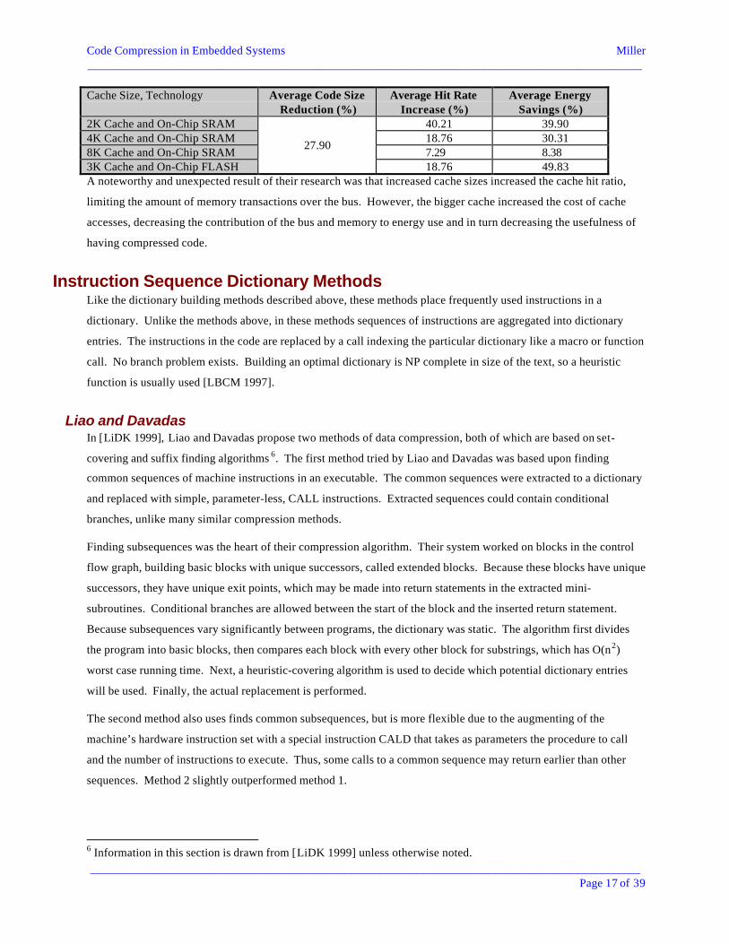
On a series of C program benchmarks, code size reduction averaged 28% and ranged from 11% to 61%. Cache hit

ratio improvement averaged 19%, ranging from 0% to 34%, with similar figures for energy use reduction being 30%

and 8% to 53%. Shown below are average results taken over a set of C program benchmarks for compression ratios,

hit rates, and energy use reductions:


____________________________________________________________________________________________ of 39

Cache Size, Technology Average Code SizeReduction (%)

Average Hit RateIncrease (%)

Average EnergySavings (%)

2K Cache and On-Chip SRAM 40.21 39.904K Cache and On-Chip SRAM 18.76 30.318K Cache and On-Chip SRAM 7.29 8.383K Cache and On-Chip FLASH

27.90

18.76 49.83A noteworthy and unexpected result of their research was that increased cache sizes increased the cache hit ratio,

limiting the amount of memory transactions over the bus. However, the bigger cache increased the cost of cache

accesses, decreasing the contribution of the bus and memory to energy use and in turn decreasing the usefulness of

having compressed code.

Instruction Sequence Dictionary MethodsLike the dictionary building methods described above, these methods place frequently used instructions in a

dictionary. Unlike the methods above, in these methods sequences of instructions are aggregated into dictionary

entries. The instructions in the code are replaced by a call indexing the particular dictionary like a macro or function

call. No branch problem exists. Building an optimal dictionary is NP complete in size of the text, so a heuristic

function is usually used [LBCM 1997].

Liao and DavadasIn [LiDK 1999], Liao and Davadas propose two methods of data compression, both of which are based on set-

covering and suffix finding algorithms 6. The first method tried by Liao and Davadas was based upon finding

common sequences of machine instructions in an executable. The common sequences were extracted to a dictionary

and replaced with simple, parameter-less, CALL instructions. Extracted sequences could contain conditional

branches, unlike many similar compression methods.

Finding subsequences was the heart of their compression algorithm. Their system worked on blocks in the control

flow graph, building basic blocks with unique successors, called extended blocks. Because these blocks have unique

successors, they have unique exit points, which may be made into return statements in the extracted mini-

subroutines. Conditional branches are allowed between the start of the block and the inserted return statement.

Because subsequences vary significantly between programs, the dictionary was static. The algorithm first divides

the program into basic blocks, then compares each block with every other block for substrings, which has O(n2)

worst case running time. Next, a heuristic-covering algorithm is used to decide which potential dictionary entries

will be used. Finally, the actual replacement is performed.

The second method also uses finds common subsequences, but is more flexible due to the augmenting of the

machine’s hardware instruction set with a special instruction CALD that takes as parameters the procedure to call

and the number of instructions to execute. Thus, some calls to a common sequence may return earlier than other

sequences. Method 2 slightly outperformed method 1.

6 Information in this section is drawn from [LiDK 1999] unless otherwise noted.


____________________________________________________________________________________________ of 39

Because returns from the function were implicit by the number of instructions executed, if the mini-subroutine

contained branches, one side of the branch may need to have NOPs inserted to make the number of instructions

executed equal in both branches. The CALD instruction required a counter of instructions left to execute and a stack

of subroutines be added to the CPU.

The compression methods were tested using TI’s TMC320C25 compiler. Method II outperformed Method I by

approximately 2-5% on the sample programs compressed. Compression ratios on unix compress and gzip, and jpeg

programs were .923, .789, .863 using method I and .967, 0.928, and 0.931 using method II. Compression times

ranged from 0.410s to 93.600s seconds on 811 and 9663 instruction programs for Method I, with similar results for

Method II.

A unique idea was taken from Hennessy and Patterson’s 90/10 locality rule that about 90% of the execution time is

spent in 10% of the code. Therefore, compressing only the 90% least used code was tried. This was found to

degrade compression ratios by 2-3%. When compared to execution speed of uncompressed programs, compressing

only the least-used code yielded a 1-2% versus 15-17% for complete compression.

Lefurgy et al[LBCM 1997] describes an algorithm that builds a dictionary of sequences of instructions7. Once repeating

sequences were identified, a greedy heuristic function was used that selects for the largest immediate savings.

Unlike [LiDK 1999], sequences were limited to one basic block. Instruction sequences were immediately replaced

by their dictionary index. Codewords of size 16, 12, 8, and 4 bits were tried.

Relative branches were not compressed because distances between instructions could change after a compression

pass requiring a readjustment process that had been shown to be NP-complete. However, indirect branches that take

their target from a register were compressed. Because codewords were smaller than the CPU’s smallest branch

alignment (e.g. 4 bit codewords are 8 times smaller than the normal 32-bit branch alignment), the control unit of the

processor was modified to treat branches as being aligned with codewords. Because uncompressed instructions

were larger than those compressed, this reduced the range of some branches, so jump tables were created to handle

jumps requiring them.

Experiments were run on the PowerPC instruction set, compiling with gcc 2.7.2. Of the plethora of results, one

interesting result was that dictionary entries equal to or larger than 8 instructions tended to decrease compression

ratio, due to the destruction of smaller, useful dictionary entries by the greedy algorithm. Even when dictionary

entries holding 4 instructions with dictionaries holding 16, 32, or 64 entries were used, 8%, 12%, and 16%

(respectively) of code from programs were removed. When using variable length codewords with shorter

codewords for more frequent encodings, code reduction of 30% to 50% was achieved, with compression ratios very

close to that of the unix command compress. Maximum number of dictionary entries had the greatest effect on code

reduction followed by allowing shorter codewords.

7 Information in this section is drawn from [LBCM 1997] unless otherwise noted.


____________________________________________________________________________________________ of 39

Experiments were run on the PowerPC instruction set. One interesting result was that dictionary entries equal to or

larger than 8 instructions tended to decrease compression ratio, due to the destruction of smaller, useful dictionary

entries by the greedy algorithm. Even when 4 instruction entries in dictionaries of sizes 16, 32, or 64 were used,

8%, 12%, and 16% (respectively) of bytes from programs were removed. When using variable length codewords

with more frequent encodings assigned shorter codewords, code reduction of 30% to 50% is achieved. Maximum

number of dictionary entries had the greatest effect on code reduction followed by allowing shorter codewords.

Chen, Bird, and MudgeThe algorithm described in [ChBM 1997] also determined frequencies of instructions, this time based on only on the

binary bits of the instructions of fixed length, and only within each basic block8. A tiling method was used to

greedily select the sequences with the highest frequency, with sequences being placed in a dictionary and the

dictionary index replacing the instruction in the code.

Chen’s compression scheme differed in the location where decompression takes place: past the compression cache

on the way to the CPU core. Along this path, compressed instructions were dereferenced from the dictionary before

being passed to the CPU.

Measurements were taken using a DEC-21064-based workstation on the SPEC CINT95 and CFP95 benchmarks.

Program size reduction was measured at 45% to 60%. The focus of the paper was to measure bytes fetched from the

cache, and the miss ratio as the instruction cache (I-cache) was varied from 2K to 32K.

Compression was found to reduce the number of bytes needed by the CPU, even when only 32 dictionary entries

were formed. Chen also found that a less optimistic but more realistic measurement of performance than % bytes

needed for execution was % bus cycles used by the compressed program, which was larger than % bytes needed

because padding to fill byte boundaries was performed on each fetch. On average, the number of bytes needed was

reduced to about 50% compared to uncompressed code, while the number of cycles needed reduced to about 65%.

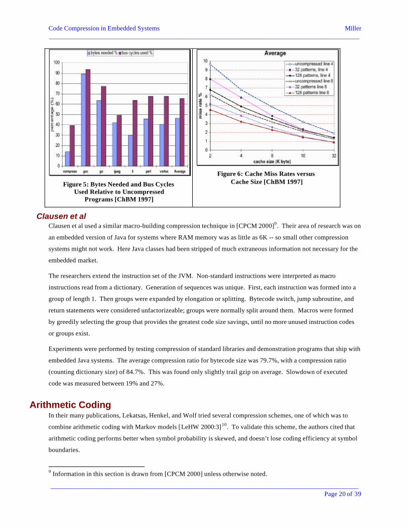
The results for integer benchmarks from the SPEC 95 benchmark suite are shown in Figure 5 below. A final finding

showed that increasing the cache size decreased the cache miss rate approximately proportional to the inverse square

root of the cache size, on average. In fact, the miss rate of programs compressed with only 128 dictionary entries

was less than that for an architecture with twice the cache size. Results for cache miss rates are compared in Figure

6 below for uncompressed code, 32 and 128 entry dictionaries, and cache line sizes of 4 and 8 instructions.

8 Information in this section is drawn from [ChBM 1997] unless otherwise noted.


____________________________________________________________________________________________ of 39

Figure 5: Bytes Needed and Bus CyclesUsed Relative to Uncompressed

Programs [ChBM 1997]

Figure 6: Cache Miss Rates versusCache Size [ChBM 1997]

Clausen et alClausen et al used a similar macro-building compression technique in [CPCM 2000]9. Their area of research was on

an embedded version of Java for systems where RAM memory was as little as 6K -- so small other compression

systems might not work. Here Java classes had been stripped of much extraneous information not necessary for the

embedded market.

The researchers extend the instruction set of the JVM. Non-standard instructions were interpreted as macro

instructions read from a dictionary. Generation of sequences was unique. First, each instruction was formed into a

group of length 1. Then groups were expanded by elongation or splitting. Bytecode switch, jump subroutine, and

return statements were considered unfactorizeable; groups were normally split around them. Macros were formed

by greedily selecting the group that provides the greatest code size savings, until no more unused instruction codes

or groups exist.

Experiments were performed by testing compression of standard libraries and demonstration programs that ship with

embedded Java systems. The average compression ratio for bytecode size was 79.7%, with a compression ratio

(counting dictionary size) of 84.7%. This was found only slightly trail gzip on average. Slowdown of executed

code was measured between 19% and 27%.

Arithmetic CodingIn their many publications, Lekatsas, Henkel, and Wolf tried several compression schemes, one of which was to

combine arithmetic coding with Markov models [LeHW 2000:3]10. To validate this scheme, the authors cited that

arithmetic coding performs better when symbol probability is skewed, and doesn’t lose coding efficiency at symbol

boundaries.

9 Information in this section is drawn from [CPCM 2000] unless otherwise noted.


____________________________________________________________________________________________ of 39

Their algorithm separated types of instructions into four groups, each group had a short prefix to identify it (shown

in parenthesis): instructions with immediates (0), branches (11), “fast dictionary instructions” (100), and

uncompressed instructions (101). Group 1 instructions were compressed using the Markov model and arithmetic

coding, group 2 instructions were compressed by rewriting them in a form without unnecessary bits common to

equal-length instructions in RISC architectures, group 3 instructions were looked up in a 256 entry table with the

stipulation that such instructions have no immediate fields. Phase 1 of compression made a pass to build the

Markov model. Phase 2 compressed group 1 instructions. Phase 3 compressed branches only, compressing the code

further still. Phase 4 patched the branch offsets that have been marked in the two previous phases.

Compression ratios of the group 2 instructions were better than for group 1. Overall compression ratios were about

0.52 to 0.56, considering code only. Different groups of instructions were present at different frequency in the code

with group 1 instructions about twice as common as groups 2 or 3, and group 4 representing only 0.6% of the code.

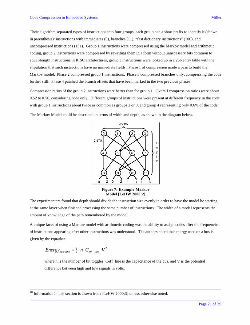
The Markov Model could be described in terms of width and depth, as shown in the diagram below.

Figure 7: Example MarkovModel [LeHW 2000:2]

The experimenters found that depth should divide the instruction size evenly in order to have the model be starting

at the same layer when finished processing the same number of instructions. The width of a model represents the

amount of knowledge of the path remembered by the model.

A unique facet of using a Markov model with arithmetic coding was the ability to assign codes after the frequencies

of instructions appearing after other instructions was understood. The authors noted that energy used on a bus is

given by the equation:

2_2

1 VCnEnergy lineefflinebus ⋅⋅⋅=−

where n is the number of bit toggles, Ceff_line is the capacitance of the bus, and V is the potential

difference between high and low signals in volts.

10 Information in this section is drawn from [LeHW 2000:3] unless otherwise noted.


____________________________________________________________________________________________ of 39

Lekatsas et al’s system assigned encoding bits so as to reduce bit toggling for more frequent codewords. At any

given state in the Markov Model, the same bit would be assigned to the most probable next transition as was the bit

along the most probable last transition used to reach the state. Reducing bit toggling for codewords reduced power

use on buses over which compressed instructions passed, with no loss to decoding performance.

Since instruction size was reduced, the amount of data transferred to the CPU for each normally 32-bit instruction

fetch could be reduced. Two methods were tried. The first was to leave the unused bits of compressed instructions

unchanged because bit toggles use energy. The second method, found to be significantly more effective at power

reduction, was to pack as much as possible of the next instruction into leftover space. Number of toggles on buses

when performing decompression before and after the I-cache was examined, and decompression after the I-cache

was found to have significant benefit.

Energy savings were found to be between 16% and 54%. If extra performance was traded to save more energy by

slowing down the clock frequency, savings ranged from 16% to 82%. Energy savings were greatest in the CPU

which benefited from reduced idle time due to cache misses, as well as through reduced bit toggles on the buses, in

the cache, and elsewhere. Energy consumption of the hardware decompression unit was negligible compared to that

used and saved in the rest of the system.

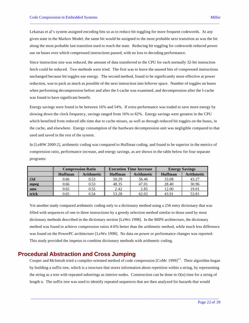
In [LeHW 2000:2], arithmetic coding was compared to Huffman coding, and found to be superior in the metrics of

compression ratio, performance increase, and energy savings, as are shown in the table below for four separate

programs:

Compression Ratio Execution Time Increase Energy SavingsHuffman Arithmetic Huffman Arithmetic Huffman Arithmetic

i3d 0.66 0.53 50.29 56.46 33.08 43.27mpeg 0.66 0.53 48.35 47.01 28.40 30.96smo 0.65 0.55 2.42 2.85 12.00 19.01trick 0.65 0.54 53.28 62.02 43.91 53.81

Yet another study compared arithmetic coding only to a dictionary method using a 256 entry dictionary that was

filled with sequences of one to three instructions by a greedy selection method similar to those used by most

dictionary methods described in the dictionary section [LeWo 1998]. In the MIPS architecture, the dictionary

method was found to achieve compression ratios 4-6% better than the arithmetic method, while much less difference

was found on the PowerPC architecture [LeWo 1998]. No data on power or performance changes was reported.

This study provided the impetus to combine dictionary methods with arithmetic coding.

Procedural Abstraction and Cross JumpingCooper and McIntosh tried a compiler-oriented method of code compression [CoMc 1999]11. Their algorithm began

by building a suffix tree, which is a structure that stores information about repetition within a string, by representing

the string as a tree with repeated substrings as interior nodes. Construction can be done in O(n) time for a string of

length n. The suffix tree was used to identify repeated sequences that are then analyzed for hazards that would


____________________________________________________________________________________________ of 39

prevent code compression, and the suffixes were split around such hazards. Next, two transformations were applied.

The first, procedural abstraction, created new procedures out of frequently repeated sequences of code and replaces

sequences with procedure calls. The second, cross jumping or “tail merging”, merged the ends of sequences that

will end by jumping to the same location by having one sequence be jumped into by sequences with similar endings.

Two abstraction techniques were used to increase the number of repeated sequences. In branch abstraction,

branches were recoded in a PC-relative form whenever possible, to identify more similar sequences and sequences

that spanned multiple blocks. The other technique, abstracting registers, renamed registers in sequences in terms of

uses and definitions within its enclosing basic block. Register renaming could then be applied to make sequences

identical to each other, and live range recoloring is used to reassign registers in blocks. A final optional

improvement was based on Patterson and Hennessy’s 90/10 principle: profiling data is used to locate the most

frequently run code, which is left uncompressed.

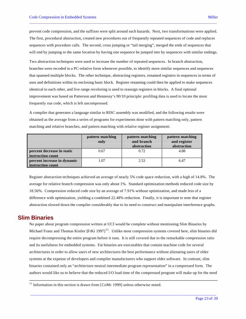
A compiler that generates a language similar to RISC assembly was modified, and the following results were

obtained as the average from a series of programs for experiments done with pattern matching only, pattern

matching and relative branches, and pattern matching with relative register assignment:

pattern matchingonly

pattern matchingand branchabstraction

pattern matchingand registerabstraction

percent decrease in staticinstruction count

0.67 0.72 4.88

percent increase in dynamicinstruction count

1.07 2.53 6.47

Register abstraction techniques achieved an average of nearly 5% code space reduction, with a high of 14.8%. The

average for relative branch compression was only about 1%. Standard optimization methods reduced code size by

18.56%. Compression reduced code size by an average of 7.91% without optimization, and made less of a

difference with optimization, yielding a combined 22.48% reduction. Finally, it is important to note that register

abstraction slowed down the compiler considerably due to its need to construct and manipulate interference graphs.

Slim BinariesNo paper about program compression written at UCI would be complete without mentioning Slim Binaries by

Michael Franz and Thomas Kistler [FrKi 1997]12. Unlike most compression systems covered here, slim binaries did

require decompressing the entire program before it runs. It is still covered due to the remarkable compression ratio

and its usefulness for embedded systems. Fat binaries are executables that contain machine code for several

architectures in order to allow users of new architectures the best performance without alienating users of older

systems at the expense of developers and compiler manufacturers who support older software. In contrast, slim

binaries contained only an “architecture neutral intermediate program representation” in a compressed form. The

authors would like us to believe that the reduced I/O load time of the compressed program will make up for the need

11 Information in this section is drawn from [CoMc 1999] unless otherwise noted.


____________________________________________________________________________________________ of 39

to generate machine code at load time. Other features of slim binaries are support for modern software engineering

paradigms of creating modules with import and export interfaces, dynamic binding, and embedding applications in

documents.

The compression scheme of slim binaries was adaptive (using an ever-growing vocabulary) and predictive, adding

items to the vocabulary before they are encountered in the source. It operated on abstract syntax trees rather than

machine code. The vocabulary began with a few basic primitive operations such as assignment, addition ,

subtraction, and procedure call. The algorithm began by parsing the source code into an abstract syntax tree (AST)

and building a symbol table. Next, the tree was traversed with the encoder building the evolving vocabulary as it

processed. For example, the AST for the procedure call P(i + 1) would be encoded using operation symbols

procedure call, addition , and data symbols procedure P, variable i , and constant 1 . The vocabulary would be

updated to include a new symbol for P(i + 1). Additional vocabulary entries would be created using prediction

heuristics, creating such symbols as i-plus-something, something-plus-one, and predicting symmetric use in the

future, i-minus-something, something-minus-one. This would make encoding of a later statement such as i + j

easier. The adaptive system allows whole branches of the AST to be processed at a time.

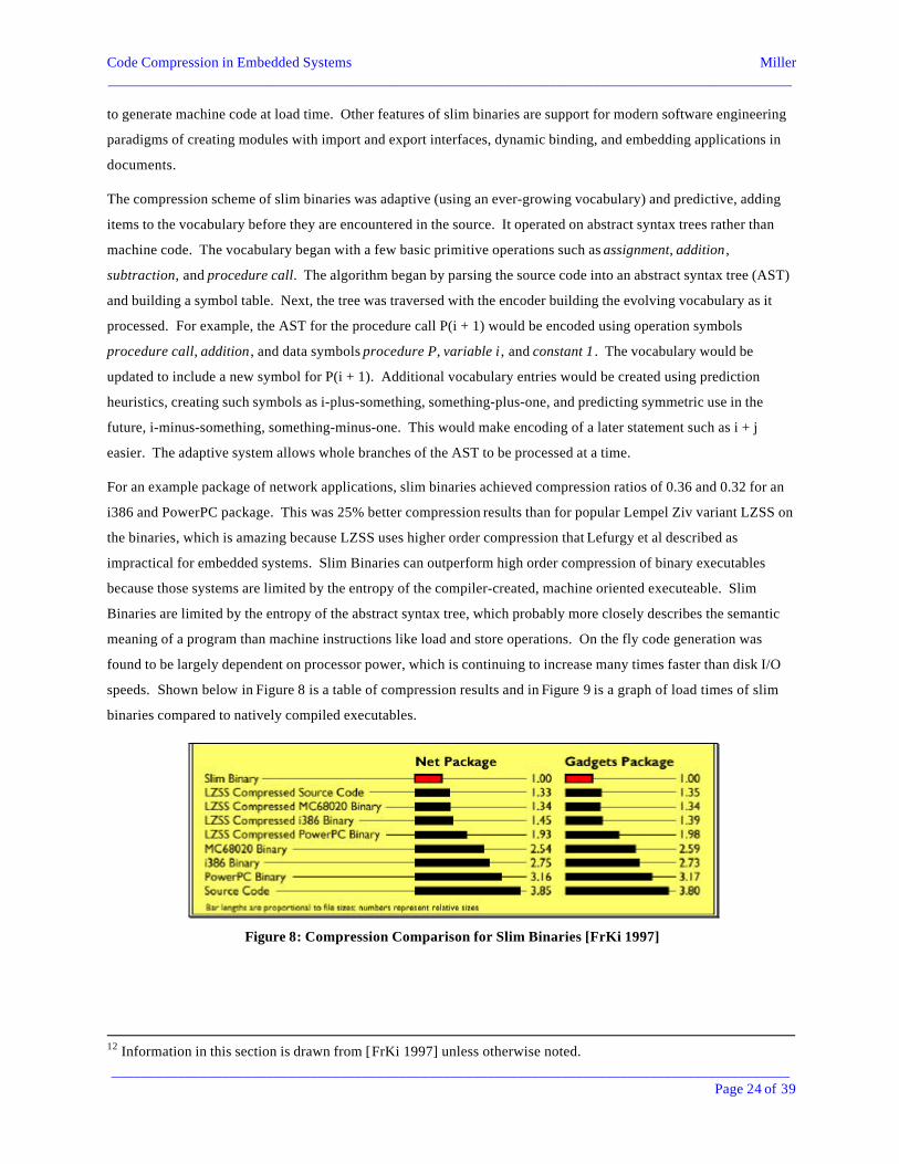
For an example package of network applications, slim binaries achieved compression ratios of 0.36 and 0.32 for an

i386 and PowerPC package. This was 25% better compression results than for popular Lempel Ziv variant LZSS on

the binaries, which is amazing because LZSS uses higher order compression that Lefurgy et al described as

impractical for embedded systems. Slim Binaries can outperform high order compression of binary executables

because those systems are limited by the entropy of the compiler-created, machine oriented executeable. Slim

Binaries are limited by the entropy of the abstract syntax tree, which probably more closely describes the semantic

meaning of a program than machine instructions like load and store operations. On the fly code generation was

found to be largely dependent on processor power, which is continuing to increase many times faster than disk I/O

speeds. Shown below in Figure 8 is a table of compression results and in Figure 9 is a graph of load times of slim

binaries compared to natively compiled executables.

Figure 8: Compression Comparison for Slim Binaries [FrKi 1997]

12 Information in this section is drawn from [FrKi 1997] unless otherwise noted.


____________________________________________________________________________________________ of 39

Figure 9: Load Times for Network Package in Slim Binaries andNative Code [FrKi 1997]


____________________________________________________________________________________________ of 39

Summary of Compression System PerformanceThe table below lists a summary of the performance of the compression systems described herein. Most authors

provided results either for overall program compression ratio or for code compression ratio, which would

presumably appear better because it did not include extra tables or models that must be part of the whole compressed

program. Performance refers to the inverse of the execution time, unless otherwise noted.

Author CompressionMethod

ProgramCompressionRatio (%)

CodeCompressionRatio (%)

EnergyRequirementChange (%)

PerformanceChange (%)

Wolfe and Chanin Huffman 65 to 75 -13 to +38Larin and Conte Huffman, stream 70 to 78 -4 to +93Larin and Conte Tailored 60 to 67 +2 to +188Larin and Conte Huffman, whole

op+11 to +225

Yoshida et al InstructionDictionary

22.7 to 54.0 -58 to -80(memory)

Jin and Chen InstructionDictionary

70 to 76 +0 to +40 (cache hitrate)

Benini et al InstructionDictionary

72 -30.31 +18.76 (cache hit rate)

Liao and Davadas SequenceDictionary

85.1 to 96.5 +15 to +17

Lefurgy et al SequenceDictionary

53 to 70

Chen et al SequenceDictionary

40 to 55 +40 to +90 (bus cycles)

Clausen et al SequenceDictionary

84.7 79.7 +19 to +27

Lekatsas et al Arithmetic 52 to 56 -19.01 to -53.81 +2.85 to +62.02Lekatsas et al Huffman 65 to 66 -12.00 to -43.91 +2.42 to +53.28Lekatsas et al Sequence

Dictionary43 to 58

Cooper and McIntosh Compiler 93 to 96Franz and Kistler Slim Binaries 32 to 36

Misconceptions about Code CompressionResearchers and computer scientists alike have several misconceptions about the efficacy of code compression.

Several misconceptions and the truths are described below.

• “Performance will decrease because decompression must be done on the fly.” In actuality, codecompression is often done by fast table lookups near the CPU, decreasing the amount of data moved on thebus from memory to the I-cache. In fact, systems that used post I-cache compression increased theeffective cache size and decreased the cache miss rate as well as the amount of data that needed to bebrought across the bus from I-cache to CPU, which increased performance [LeHW 2000:3].

• “CISC Systems tend to be more dense by design, and therefore will not benefit from code compression asmuch as RISC architectures do” [LeHW 2000:2]. Several researchers made this comment, but it wasproven wrong as far back as 1994. Kozuch and Wolfe found that the zeroth order and first order entropy ofthe Vax-11 was approximately the same as 4 RISC systems, with only the MIPS having a significantlylower entropy for zeroth order [KoWo 1994].

• “Some kind of table is needed to translate uncompressed instruction addresses to compressed instructionaddresses in order to resolve branch targets.” For researchers using dictionaries of instruction sequencesthat were called like macros, this conception did not even apply. Many researchers came up with methodsof patching branch targets and offsets during a later pass, or as in Yoshida’s work, compressing allinstructions to the same width, making branch calculations trivial [YSOO 1997].


____________________________________________________________________________________________ of 39

• In Lekatsas’ work, “appending a 3-bit preamble to uncompressed instructions may cause run-timedecompression inefficiency” [BeMN 2001]. While adding the preamble adds to the size of uncompressedinstructions, in actuality, only 0.6% of instructions are uncompressed [LeHW 2000:3]. Furthermore, thepublished results indicate that use of variable length arithmetic encoding (that includes its own 256 entryinstruction dictionary) outperforms instruction dictionary methods alone [LeHW 2000:3, LeWo 1998].

• “Variable length codewords (such as those used in ... [WoCh 1992]) are expensive to decode” [LBCM1997]. Lekatsas et al used Markov models to their advantage in developing a system that was both fast todecompress, achieved a great compression ratio, and lowered power requirements by choosing encodingsso as to minimize bit changes [LeHW 2000:3].

• “Combining 2 or more compression strategies does not yield better compression” [LaCo 1999]. Actually,Lekatsas et al combined 256-entry sequence dictionary and arithmetic coding methods to achieve some ofthe best compression ratios of the papers surveyed [LeHW 2000:3]. Just using a dictionary with 256entries alone did not produce as good results [LeWo 1998, LeHW 2000:3]. In fact, gcc was able to use7927 entry instruction sequence dictionary, more than most instruction sequence dictionaries provided, soincluding an additional compression scheme with any one of them would be likely to reduce code size[LBCM 1997].

• “Higher order compression techniques (Lempel-Ziv, etc) would be too expensive for implementation inembedded systems” and this limits code compressibility in embedded systems [KoWo 1994]. As MichaelFranz discovered, it is much more effective to compress an intermediate representation of the program, thanit is to compress the executable [FrKi 1997].

• “My results are typical.” Many researchers presented their compression results based on realimplementations performing compression on a particular architecture. While it is important to have resultsfrom an implementation, Kozuch and Wolfe demonstrated that compression ratios vary by as much as 10%between architectures [KoWo 1994]. The good results produced a compression system on an architecturemay be specific only to that architecture.

• “Code compression is an indicator of a compression performance.” For exactly half of the compressionsystems surveyed, the authors reported the code compression ratios of the compression systems. Oftenthese systems required auxiliary information be added to programs in order for them to work under thecompression system such as a dictionary mapping indexes to instructions or instruction sequences. In ourown implementation below, we demonstrate that code compression ratio is not a useable indicator ofoverall compression ratios. An impressive-looking code compression ratio of 0.5000 can hide an overallprogram size increase.

ImplementationIn order to verify the results of other researchers, a code compression system was developed. This system is based

on the work of Yoshida et al, extending their system to have multiple dictionaries.

Like Yoshida’s work, the compression system first reads a program of N instructions and makes a list of n unique

instructions. In addition, it determines the frequency at which each instruction occurs, then sorts the list of n unique

instructions in order of frequency. Instructions are then placed in dictionaries of varying sizes, with the most

frequent instructions being placed in the smallest dictionaries. Dictionaries always had a number of entries that was

a power of 2.

In the original code, the original machine instructions are then replaced by a prefix that references the dictionary in

which the instruction appears, followed by the index into the dictionary of the instruction. The compression system

was tried with 1, 2, 3, and 4 dictionaries. For 3 dictionaries, the two smaller dictionaries were assumed to have a 2

bit prefix while the third was assumed to have a 1 bit prefix.

Two programs were created. One program, dcompress.py, was a compressor based on having three-dictionaries.

When run on machine instructions, the compressor produced a file containing the dictionaries used for compression


____________________________________________________________________________________________ of 39

and a file containing the compressed code. A corresponding decompression system would need to be implemented

in hardware, and would load the dictionaries into special decompression tables. The compressed code would be

stored back into the executable file.

The second program, dcalculate.py, calculated the size of the compressed code and code compression ratios that

would be achieved for various sized dictionaries if the algorithm above was applied. dcalculate.py was useful for

examining how the number of dictionaries affected compression.

Source code for both programs is included in appendix B: source code. Programs were written in the Python

programming language.

It is important to note that having multiple dictionary sizes creates varying length codewords, which in turn

necessitates a method for translating uncompressed addresses to compressed addresses. Wolfe and Chanin used a

translation table that mapped to blocks and added about 3.5% to the program size [WoCh 1992]. Larin and Conte’s

also used a table, but mapped uncompressed target addresses to compressed target address, adding 15.5% to the size

of the program [LaCo 1999]. A complete implementation of a dictionary compression scheme as described here

would also need such a table, but was not implemented here.

Generating Benchmark DataTen programs on the Sun SPARC architecture under the operating system SunOS 5.7 were selected as benchmarks

based on their popularity across unix platforms and their variety in terms of uncompressed executable size. SunOS

5.7 saves unix programs in the ELF binary format. For each program, the program “objcopy” was run with the -j

switch to extract the code segments of programs, called the “.text” segments [terran.txt]. The command “readelf”

was run with the “-l” switch on each result to determine the size of ELF headers in the objcopy’s output by

subtracting the number given for the VirtualAddress from the number given for Entry Point [readelf.html]. Finally,

the ELF headers were removed from the files along with any data that came after the number given by readelf for

the FileSize of the .text segment [terran.txt]. The resulting data was treated as being just the machine instructions of

the programs’ code segments.

The table below shows the programs used as benchmarks, the size of the executables, the size of code, the number of

unique instructions in the program, and the percentage of instructions that were unique (appeared for the first time)

in the programs. The version of the programs is listed if it was available; otherwise, the version of the operating

system, SunOS 5.7, is listed.


____________________________________________________________________________________________ of 39

Program Name Version File Size(bytes)

Code Size(bytes)

UniqueMachineInstructions

% UniqueInstructions

echo SunOS 5.7 5680 1564 246 62.92%compress SunOS 5.7 16024 8464 1288 60.87%patch SunOS 5.7 38328 21092 2114 40.09%ftp SunOS 5.7 73840 48904 4503 36.83%gzip 1.2.4 124736 90236 2532 11.22%vi SunOS 5.7 208204 155208 12705 32.74%gcc 2.8.1 417792 177724 2737 6.16%vim 5.3 684500 539736 30877 22.88%ssh2 2.4.0 4927672 507376 30997 24.44%emacs 20.4 8520132 1092588 45186 16.54%

SUM 15016908 2642892 133185 20.16%

Two very important results are seen in this table. First, [YSOO 97] indicated that when a table of unique

instructions was created, the authors needed only 12 bits to address the table. Hence, only 2^12 = 4096 or fewer

unique instructions existed in their benchmarks. In contrast, it was found that up to 45186 unique instructions

existed in executables in our benchmarks, thus for the Solaris architecture, dictionaries needed up to 16 bit indexes.

Since compression required replacing each instruction with a prefix and index, this meant that compression ratios for

the architecture and benchmark set tried here would not look as Yoshida’s results, or that Yoshida only tested rather

small programs.

The second important result is that the percentage of unique instructions appearing in programs varies significantly.

One particular program, gcc, had the most frequent instruction appearing 21280 times, while the next three most

frequent instructions appeared 2734, 1050, and 698 times. The four most frequent instructions in vi, on the other

hand, appeared 1907, 1029, 464, and 452 times.

ResultsAppendix A: Result Data includes tables listing the compressed code size, code compression ratio, and overall

program compression ratios for each of the benchmark programs tested. Figure 10 below shows the average code

compression ratio for various dictionaries. Figure 11 below is a similar graph of average overall compression ratios

(note that we do not include a means to translate uncompressed branch target addresses to compressed branch

addresses).


____________________________________________________________________________________________ of 39

Average Code Compression Ratio

0.0000

0.1000

0.2000

0.3000

0.4000

0.5000

0.6000

6553

6

1x65

536

4x65

536

16x6

5536

64x6

5536

256x

6553

6

1x12

8x65

536

1x25

6x65

536

4x25

6x65

536

4x51

2x65

536

16x1

28x6

5536

16x2

56x6

5536

16x5

12x6

5536

32x2

56x6

5536

32x5

12x6

5536

32x1

024x

6553

6

64x2

56x6

5536

64x5

12x6

5536

16x6

4x51

2x65

536

16x1

28x4

096x

6553

6

1x64

x512

x655

36

4x64

x512

x655

36

1x12

8x25

6x65

536

1x12

8x51

2x65

536

1x12

8x10

24x6

5536

Dictionary Size

Compression Ratio

MEAN

Figure 10: Average Code Compression Ratio

Average Overall Compression Ratio

0.7800

0.8000

0.8200

0.8400

0.8600

0.8800

0.9000

0.9200

6553

6

1x65

536

4x65

536

16x6

5536

64x6

5536

256x

6553

6

1x12

8x65

536

1x25

6x65

536

4x25

6x65

536

4x51

2x65

536

16x1

28x6

5536

16x2

56x6

5536

16x5

12x6

5536

32x2

56x6

5536

32x5

12x6

5536

32x1

024x

6553

6

64x2

56x6

5536

64x5

12x6

5536

16x6

4x51

2x65

536

16x1

28x4

096x

6553

6

1x64

x512

x655

36

4x64

x512

x655

36

1x12

8x25

6x65

536

1x12

8x51

2x65

536

1x12

8x10

24x6

5536

Dictionary Size

Compression Ratio

MEAN

Figure 11: Average Overall Compression Ratio


____________________________________________________________________________________________ of 39

A few observations and results are worth mentioning. First, code compression ratio is not a very good indicator of

overall compression ratio. Many authors in the papers surveyed reported only code compression ratios even when

their compression schemes seemed to require a large dictionary and/or a table for resolving branch addresses. Such

figures belie the actual compression ratio that the system could produce. Second, having multiple dictionaries

improves code compression. In fact, with four tables of sizes 16, 128, 4096, and 65536, the average code

compression ratio is 30% better than using a single table. Third, having multiple dictionaries improves overall

compression ratios. The same set of four tables produces an average overall compression ratio 8.23% better than a

single table scheme. Fourth, the gains made by adding more dictionaries tends to decrease substantially after the

second table is added. Moving from a single dictionary to two dictionaries with 256 and 65536 entries, the code

compression ratio improves by 6.18%. Moving from said two dictionaries to three dictionaries with 32, 512, and

65536 entries only improves the overall compression ratio by 1.15%. Moving from three dictionaries to the highest

compressing system tried, four dictionaries with 16, 128, 4096, and 65536 entries, only improves the code

compression ratio by 1.04%.

The code compression ratio and overall compression ratio of four selected programs are shown below in figures 12

and 13. A few novel observations may be made. First, code compression ratios tend to be small (better) for very

small programs and programs that have a low percentage of unique instructions. One would tend to expect this

because the majority of compressed instructions would refer to smaller dictionaries that could be addressed with

fewer bits. The trends in figure 13 reiterates why code compression ratios are not useful for reporting results.

Overall compression ratios are very high (worse) for small programs. Due to the overhead of storing a dictionary,

compressed programs may be even larger than uncompressed programs. Overall compression ratios are lower for

medium to large programs that have a lower percentage of unique instructions


____________________________________________________________________________________________ of 39

Code Compression Ratios for Four Programs

0.0000

0.1000

0.2000

0.3000

0.4000

0.5000

0.6000

6553

6

1x65

536

4x65

536

16x6

5536

64x6

5536

256x

6553

6

1x12

8x65

536

1x25

6x65

536

4x25

6x65

536

4x51

2x65

536

16x1

28x6

5536

16x2

56x6

5536

16x5

12x6

5536

32x2

56x6

5536

32x5

12x6

5536

32x1

024x

6553

6

64x2

56x6

5536

64x5

12x6

5536

16x6

4x51

2x65

536

16x1

28x4

096x

6553

6

1x64

x512

x655

36

4x64

x512

x655

36

1x12

8x25

6x65

536

1x12

8x51

2x65

536

1x12

8x10

24x6

5536

Table Size

Compression Ratio

echo

vi

gcc

emacs

Figure 12: Code Compression Ratios for Selected Programs

Overall Compression Ratios for Four Programs

0.0000

0.2000

0.4000

0.6000

0.8000

1.0000

1.2000

6553

6

1x65

536

4x65

536

16x6

5536

64x6

5536

256x

6553

6

1x12

8x65

536

1x25

6x65

536

4x25

6x65

536

4x51

2x65

536

16x1

28x6

5536

16x2

56x6

5536

16x5

12x6

5536

32x2

56x6

5536

32x5

12x6

5536

32x1

024x

6553

6

64x2

56x6

5536

64x5

12x6

5536

16x6

4x51

2x65

536

16x1

28x4

096x

6553

6

1x64

x512

x655

36

4x64

x512

x655

36

1x12

8x25

6x65

536

1x12

8x51

2x65

536

1x12

8x10

24x6

5536

Table Size

Compression Ratio

echo

vi

gcc

emacs

Figure 13: Overall Compression Ratios for Selected Programs


____________________________________________________________________________________________ of 39

In [LBCM 1997], it was reported that the 1% most frequent instructions account for 30% the size of machine code,

and the 10% most frequent instructions account for 66% of the size of code. The program dcalculate.py was used to

examine the number of instructions that occurred at what frequency. For the ten benchmark programs, the

percentage of the size of code accounted for by the 1% most frequent unique instructions and the 10% most frequent

unique instructions was calculated as well as for the 1% most frequent total instructions and the 10% most frequent

total instructions. Percentages for most frequent unique instructions were determined by dividing the number of

unique instructions by 100 and 10, respectively. Percentages for the most frequent total instructions were

determined by dividing the total number of instructions by 100 and 10, respectively. Results are shown in the table

below.

ProgramName

File Size Code Size UniqueMachineInstructions

One PercentUniqueInstructions

Ten PercentUniqueInstructions

One PercentTotalInstructions

Ten PercentTotalInstructions

echo 5680 1564 246 6.65% 39.64% 13.04% 46.80%compress 16024 8464 1288 13.66% 38.89% 17.82% 46.74%patch 38328 21092 2114 21.58% 53.31% 32.68% 68.52%ftp 73840 48904 4503 25.96% 56.87% 37.54% 72.65%gzip 124736 90236 2532 40.45% 79.64% 78.09% 98.78%vi 208204 155208 12705 33.96% 61.33% 46.43% 77.26%gcc 417792 177724 2737 72.07% 90.06% 92.88% 100.00%vim 684500 539736 30877 43.48% 70.93% 60.96% 87.12%ssh2 4927672 507376 30997 38.14% 68.04% 55.42% 85.56%emacs 8520132 1092588 45186 48.53% 77.68% 72.13% 93.46%

MEAN 34.45% 63.64% 50.70% 77.69%

Our results tend to agree with those reported in [LBCM 1997] for programs larger than 50K. We found on average

that the 1% most frequent unique instructions account for approximately 34.45% of the code size, and the 10% most

frequent unique instructions account for approximately 63.65% the size of the code.

The distribution of instructions is shown below for the program ftp in a list of pairs. The first element in each pair

reports the frequency at which one or more unique instructions occurred. The second element reports the number of

unique instructions to occur that many times in the program. The program ftp had 12226 total instructions of which

4503 were unique.

(332, 1), (268, 1), (250, 1), (198, 1), (161, 1), (110, 1), (103, 1), (96, 1), (95, 1), (83, 1), (81, 1),

(74, 2), (73, 2), (67, 1), (63, 1), (48, 2), (46, 1), (44, 2), (42, 1), (41, 1), (39, 1), (38, 1), (37, 2), (35,

2), (34, 1), (32, 2), (31, 1), (30, 1), (29, 4), (28, 2), (27, 5), (26, 5), (25, 4), (24, 1), (23, 2), (22, 4),

(21, 8), (20, 5), (19, 2), (18, 7), (17, 5), (16, 5), (15, 13), (14, 14), (13, 17), (12, 17), (11, 18), (10,

21), (9, 23), (8, 23), (7, 42), (6, 52), (5, 82), (4, 132), (3, 187), (2, 552), (1, 3216)

(frequency, number unique instructions) for ftp


____________________________________________________________________________________________ of 39

The distribution of instructions for ftp reiterates the uneven rate at which machine instructions appear in a typical

program.

ConclusionCode compression can be employed to shrink the storage and memory requirements of programs. Additionally,

power requirements may lessen and performance may increase through increased effective cache sizes, fewer and

smaller bus transactions, and optimized bit patterns sent across the bus. These combine to produce embedded

systems that cost and weigh less, are smaller, and run faster. Code compression remains an active area of research

in 2002.

Two programs for code compression were developed and tested on 10 benchmark programs. Several original

findings were found. On the SPARC architecture, as many as 45186 unique instructions appear per program, not

4096 as reported for an architecture used in [YSOO 1997]. The percentage of unique instructions varies per

program with 60% being typical for small executables around 10K in size, 20% to 30% for 100K executables, and

20% for multi-megabyte executables. Code compression ratios are not a good indicator of overall compression

ratios. Both average code compression ratios and average overall compression ratios are improved when

dictionaries of several sizes are used. While two dictionaries produces much better results than just one dictionary,

the benefits of more than two dictionaries is not substantial.

Code compression ratios are lower (thus, better) for smaller programs and programs with a lower percentage of

unique instructions; however, overall compression ratios follow a different trend. Overall compression ratios are

better for medium to large programs with a lower percentage of unique instructions. Code compression ratios are

not a good indicator of compression performance. Finally, the frequency at which instructions appear in the

programs is highly skewed with the 1% most frequent unique instructions accounting for about 34% of the code

size, and the 10% most frequent unique instructions accounting for about 64% of the code size.


____________________________________________________________________________________________ of 39

References• [BeMN 2001] Cached-code compression for energy minimization in embedded processors. Luca Benini,

Alberto Macii, Alberto Nannarelli. Proceedings of the 2001 international symposium on Lowpower electronics and design. August 2001.

• [ChBM 1997] The Impact of Instruction Compression on I-cache Performance. I-Cheng K. Chen, Peter L.Bird, Trevor Mudge. Technical Report CSE-TR-330-97, University of Michigan, 1997.

• [CPCM 2000] Java Bytecode Compression for Low-End Embedded Systems. Lars Raeder Clausen, UlrikPagh Schultz, Charles Consel, and Gilles Muller. ACM Transactions on ProgrammingLanguages and Systems. May 2000.

• [CoMc 1999] Enhanced Code Compression for Embedded RISC Processors. Keith D. Cooper andNathaniel McIntosh. Proceedings of the 1999 International Conference on ProgrammingLanguage Design and Implementation.

• [Doug] The Compression Cache: Using On-Line Compression to Extend Physical Memory. FredDouglis . Matsushita Information Technology Laboratory.

• [Fano 1961] Transmission of Information. R.M. Fano. Cambridge, MA: MIT Press 1961.• [FrKi 1997] Slim Binaries. Michael Franz and Thomas Kistler. Communications of the ACM. December

1997.• [EEFL 1997] Code Compression. Jens Ernst, William Evans, Christopher W. Fraser, Steven Luco, and

Todd A. Proebsting. Proceedings of the 1997 ACM SIGPLAN conference on Programminglanguage design and implementation. May 1997.

• [HePa 1990] Computer Architecture: A Quantitative Approach . J.L. Hennessy and D.A. Patterson.Morgan Kaufman Publishers, 1990.

• [JiCh 2000] Instruction Cache Compression for Embedded Systems. Yujia Jin and Rong Chen. 2000.• [KoWo 1994] Compression of Embedded System Programs. Michael Kozuch and Andrew Wolfe.

Proceedings of the IEEE International Conference on ICCD. 1994.• [LaCo 1999] Compiler-Driven Cached Code Compression Schemes for Embedded ILM Processors. Sergei

Y. Larin and Thomas M. Conte. Proceedings of the 32nd Annual International Symposium ofMicroarchitecture, 1999.

• [LBCM 1997] Improving Code Density Using Compression Techniques. Charles Lefurgy, Peter Bird, I-Cheng Chen, and Trevor Mudge. Proceedings of the 30th Annual International Symposiumon Microarchitecture. December 1997.

• [LeHW 2000] Arithmetic Coding for Low Power Embedded System Design. Haris Lekatsas, Jörg Henkel,and Wayne Wolf. Princeton University, NEC USA, 2000.

• [LeHW 2000:2] Code Compression as a Variable in Hardware/Software Co-Design. Haris Lekatsas, JörgHenkel, Wayne Wolf. International Workshop on Hardware/Software Co-Design, 2000.

• [LeHW 2000:3] Code Compression for Low Power Embedded System Design. Haris Lekatsas, Jörg Henkel,and Wayne Wolf. Department of Electrical Engineering Princeton University.

• [LeHW 2001] H/S Embedded Systems: Design and simulation of a pipelined decompression architecture forembedded systems. Haris Lekatsas, Jörg Henkel, Wayne Wolf. Proceedings of theinternational symposium on Systems synthesis. September 2001.

• [LeWo 1998] Code Compression for Embedded Systems. Haris Lekatsas and Wayne Wolf. Department ofElectrical Engineering Princeton University, 1998.

• [LiDK 1999] A text-compression-based method for code size minimization in embedded systems. StanLiao, Srinivas Devadas, Kurt Keutzer. ACM Transactions on Design Automation ofElectronic Systems. January 1999

• [LiWu 2000] A Low-Power CAM Design for LZ Data Compression. Kun-Jin Lin and Cheng-Wen Wu.IEEE Transactions on Computers. October 2000.

• [readelf.html] readelf. http://wildsau.idv.uni-linz.ac.at/~k3032e4/virus-writing-HOWTO/_html/readelf.html.• [Sayo 2000] Introduction to Data Compression, 2nd edition . Khalid Sayood. Morgan Kaufmann

publishers. 2000.• [terran.txt] http://hcunix.org/hcunix/terran.txt.• [ViZA 2000] Dynamic Zero Compression for Cache Energy Reduction. Luis Villa, Michael Zhang, and

Krste Asanovic. 33rd International Symposium on Microarchitecture, December 2000.


____________________________________________________________________________________________ of 39

• [WoCh 1992] Executing Compressed Programs on An Embedded RISC Architecture. Andrew Wolfe andAlex Chanin. Proceedings of the 25th Annual International Symposium on MicroArchitecture, pp81-91. Dec. 1992.

• [YSOO 1997] An Object Code Compression Approach to Embedded Processors. Yukihiro Yoshida, Bae-Yu Song, Hiroyuki Okuhata, Takao Onoye, and Isao Shirakawa. Proceedings of the 1997International Symposium on Lower Power Electronics Design. 1997.

• [YSOO 1996] Low-Power Consumption Architecture for Embedded Processor. Yukihiro Yoshida, Bae-YuSong, Hiroyuki Okuhata, Takao Onoye, and Isao Shirakawa. 2nd International Conference onASIC. 1996.


____________________________________________________________________________________________ of 39

Appendix A: Result DataThe following 7 pages contain the complete result data found for the benchmark programs.


____________________________________________________________________________________________ of 39

Appendix B: Source CodeThe following 11 pages contain the source code for the programs dcount.py and dcompress.py and the module

compr_inst.py that were used to collect data and perform compression.


____________________________________________________________________________________________ of 39

Appendix C: Typical Program OutputThe following 4 pages show the output for the program dcompress.py when run on the machine code for the

program vim.

Code Compression in Embedded Systems -...

Documents

Transcript of Code Compression in Embedded Systems -...