1

Chapter 9 – Linear DifferentialEquations

Outline9.1 An Introduction to Continuous Dynamical Systems9.2 The Complex Case: Euler’s Formula9.3 Linear Differential Operators and Linear Differential Equations

2

9.1 An Introduction to Continuous Dynamical Systems

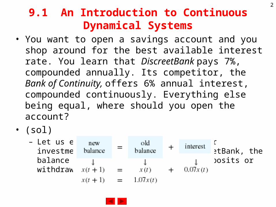
• You want to open a savings account and you shop around for the best available interest rate. You learn that DiscreetBank pays 7%, compounded annually. Its competitor, the Bank of Continuity, offers 6% annual interest, compounded continuously. Everything else being equal, where should you open the account?

• (sol)– Let us examine what will happen to your investment at the two banks. At

DiscreetBank, the balance grows by 7% each year if no deposits or withdrawals are made.

3

Example 1

– This equation describes a discrete linear dynamical system with one component. The balance after t years is x(t)=(1.07)tx0. The balance grows exponentially with time.

– At the Bank of Continuity, by definition of continuous compounding, the balance x(t) grows at an instantaneous rate of 6% of the current balance:

– Here, we use a differential equation to model a continuous linear dynamical system with one component. We will solve the differential equation in two ways, by separating variables and by making an educated guess.

– Let us try to guess the solution. We think about an easier problem first. Do we know a function x(t) that is its own derivative: dx/dt = x? You may recall from calculus that x(t)=et is such a function. (Some people define x(t)=et by this property.) More generally, the function x(t)=Cet is its own derivative, for any constant C. How can we modify x(t)=Cet to get a function whose derivative is 0.06 times itself? By the chain rule, x(t)=Ce0.06t will do:

.06.0or ),( balance of %6 xdt

dxtx

dt

dx

).(06.006.0)( 06.006.0 txCeCedt

d

dt

dx tt

4

Example 1 (II)

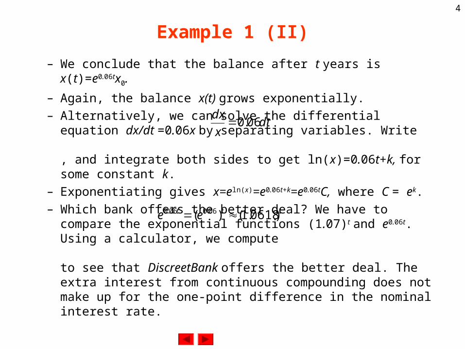
– We conclude that the balance after t years is x(t)=e0.06tx0.

– Again, the balance x(t) grows exponentially.

– Alternatively, we can solve the differential equation dx/dt =0.06x by separating variables. Write , and integrate both sides to get ln(x)=0.06t+k, for some constant k.

– Exponentiating gives x=eln(x)=e0.06t+k=e0.06tC, where C = ek.

– Which bank offers the better deal? We have to compare the exponential functions (1.07)t and e0.06t. Using a calculator, we compute

to see that DiscreetBank offers the better deal. The extra interest from continuous compounding does not make up for the one-point difference in the nominal interest rate.

dtx

dx06.0

ttt ee )0618.1()( 06.006.0

5

Exponential growth and decay

• Consider the linear differential equationwith initial value x0 (k is an arbitrary constant). The solution is

The quantity x will grow or decay exponentially (depending on the sign of k).

,kxdt

dx

.)( 0xetx kt

6

Linear Dynamical System

• A linear dynamical system can be modeled by

or

A and B are n×n matrices, where n is the number of components of the system.

model), (discrete )()1( txBtx

model), s(continuou xAdt

xd

7

Example 2

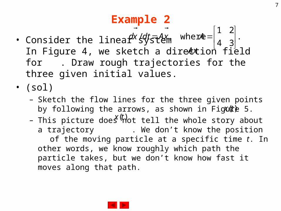
• Consider the linear systemIn Figure 4, we sketch a direction field for . Draw rough trajectories for the three given initial values.

• (sol)– Sketch the flow lines for the three given points by following the arrows,

as shown in Figure 5.

– This picture does not tell the whole story about a trajectory . We don’t know the position of the moving particle at a specific time t. In other words, we know roughly which path the particle takes, but we don’t know how fast it moves along that path.

.34

21 where,/

AxAdtxd

xA

)(tx

)(tx

8

Example 2 (II)

9

Example 2 (III)

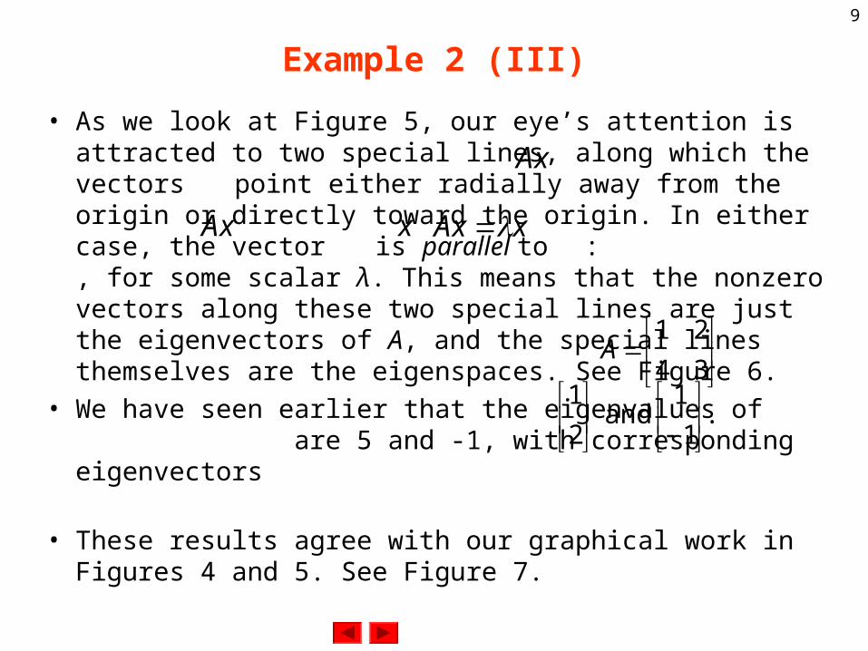
• As we look at Figure 5, our eye’s attention is attracted to two special lines, along which the vectors point either radially away from the origin or directly toward the origin. In either case, the vector is parallel to : , for some scalar λ. This means that the nonzero vectors along these two special lines are just the eigenvectors of A, and the special lines themselves are the eigenspaces. See Figure 6.

• We have seen earlier that the eigenvalues of are 5 and -1, with corresponding eigenvectors

• These results agree with our graphical work in Figures 4 and 5. See Figure 7.

xA

xA

x

xxA

34

21A

.1

1 and

2

1

10

Example 2 (IV)

11

Example 3

• Find all solutions of the system

• (sol)– The two differential equations

are unrelated, or uncoupled; we can solve them separately,

Thus,

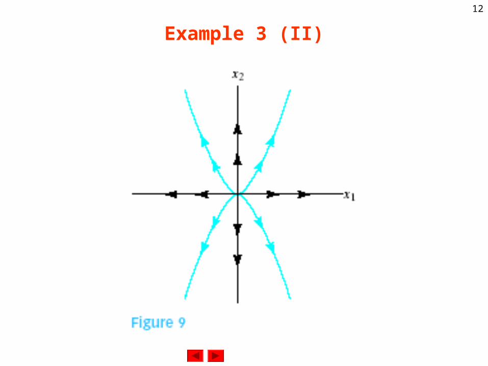
– Both components of grow exponentially, and the second one will grow faster than the first. In particular, if one of the components is initially 0, it remains 0 for all future times. In Figure 9, we sketch a rough phase portrait for this system.

.30

02x

dt

xd

22

11 3 and 2 x

dt

dxx

dt

dx

).0()( and ),0()( 23

212

1 xetxxetx tt

.)0(

)0()(

23

12

xe

xetx

t

t

)(tx

12

Example 3 (II)

13

Example 4

• Find all solutions of the system

• (sol)– We have seen that the eigenvalues and eigenvectors of A tell us a lot

about the behavior of the solutions of the system

– The eigenvalues of A are λ1=2 and λ2=3 with corresponding eigenvectors

means that S-1AS=B, where

– We can write the system

.41

21x

dt

xd

./ xAdtxd

.1

1 and

1

221

vv

.30

02 and

11

12

BS

).()(or ,or

, as

1111

1

xSBxSdt

dxBS

dt

xdS

xSBSdt

xdxA

dt

xd

14

Example 4 (II)

– Let us introduce the notation ; note that is the coordinate vector of with respect to the eigenbasis . Then the system takes the form We found that the solutions are of the form

– Therefore, the solutions of the original system are

– We can write this formula in more general terms as

Note that c1 and c2 are the coordinates of with respect to the basis, since

)()( 1 txStc )(tc

)(tx

21,vv

.cBdt

cd

constants.arbitrary are and where,)( 21

23

12

ccce

cetc

t

t

.xAdt

xd

.1

1

1

2

11

12)()( 3

22

1

23

12

tt

t

t

ececce

cetcStx

.)( 221121 vecvectx tt

)0(x

21,vv

.)0( 2211 vcvcx

15

Example 4 (III)

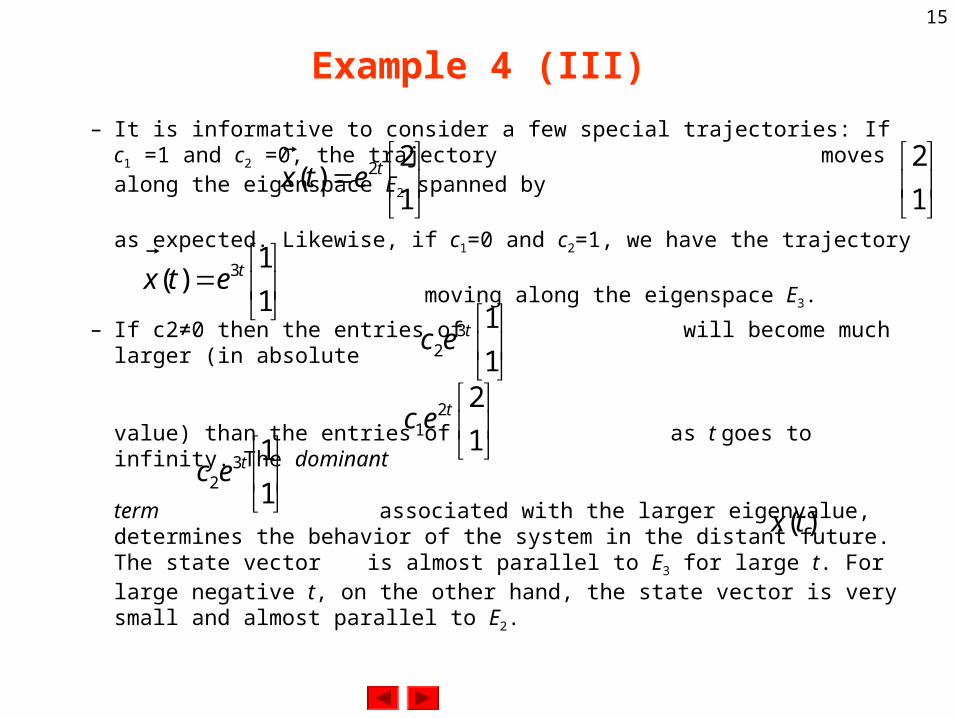
– It is informative to consider a few special trajectories: If c1 =1 and c2 =0, the trajectory moves along the eigenspace E2 spanned by

as expected. Likewise, if c1=0 and c2=1, we have the trajectory

moving along the eigenspace E3.

– If c2≠0 then the entries of will become much larger (in absolute

value) than the entries of as t goes to infinity. The dominant

term associated with the larger eigenvalue, determines the behavior of the system in the distant future. The state vector is almost parallel to E3 for large t. For large negative t, on the other hand, the state vector is very small and almost parallel to E2.

1

2)( 2tetx

1

2

1

1)( 3tetx

1

132

tec

1

221

tec

1

132

tec

)(tx

16

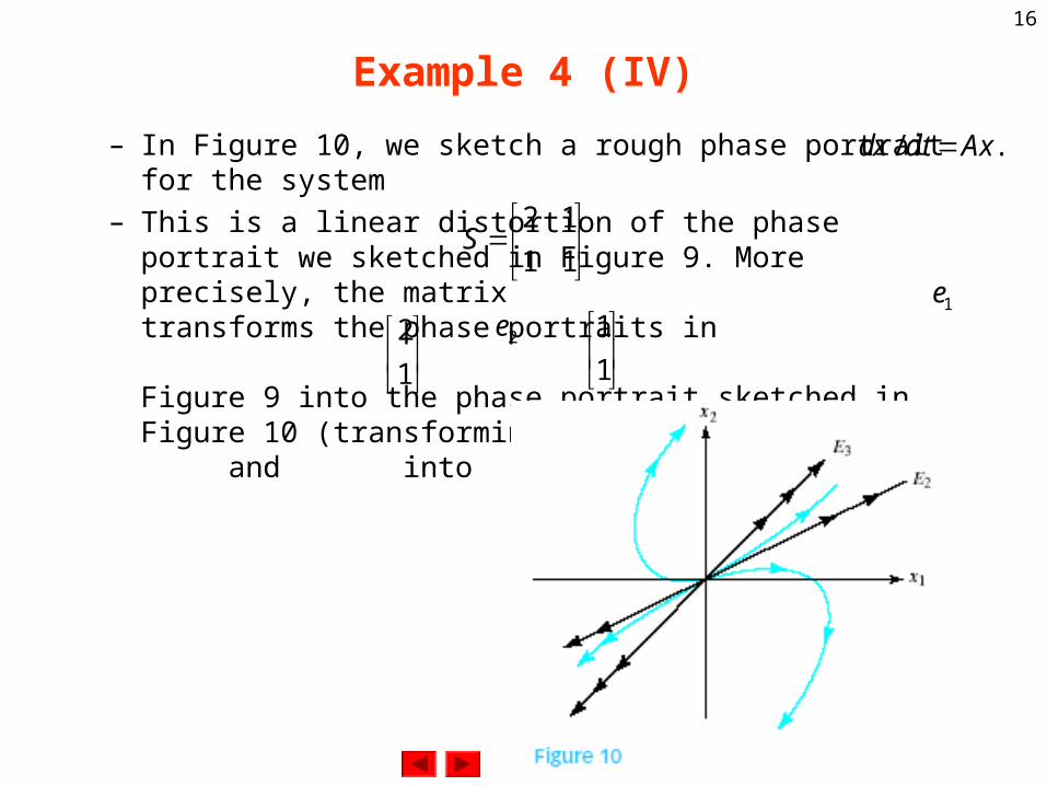
Example 4 (IV)

– In Figure 10, we sketch a rough phase portrait for the system

– This is a linear distortion of the phase portrait we sketched in Figure 9. More precisely, the matrix transforms the phase portraits in

Figure 9 into the phase portrait sketched in Figure 10 (transforming into the eigenvector and into ).

./ xAdtxd

11

12S

1e

1

2 2e

1

1

17

Continuous Dynamical Systems

• Consider the system Suppose there is a real eigenbasis for A, with associated eigenvalues λ1,... , λn. Then the general solution of the system is

Scalars c1, c2, ..., cn are the coordinates of with respect to the basisWe can write the preceding equation in matrix form as

./ xAdtxd

nvvv

,,, 21

.)( 111

nt

nt vecvectx n

.,,, 21 nvvv

0x

.

|||

|||

where,

00

00

00

00

00

00

|||

|||

)(

2101

2

1

21

2

1

2

1

n

t

t

t

nt

t

t

n

vvvSxS

e

e

e

S

c

c

c

e

e

e

vvvtx

n

n

18

Example 5

• Consider a system where A is diagonalizable over R. When is the zero state a stable equilibrium solution? Give your answer in terms of the eigenvalues of A.

• (sol)– Note that if (and only if) all eigenvalues of A are negative.

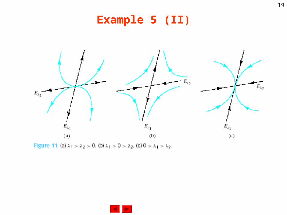
• Consider an invertible 2×2 matrix A with two distinct eigenvalues λ1>λ2. Then the phase portrait of looks qualitatively like one of the three sketches in Figure 11. We observe stability only in Figure 11(c).

• Consider a trajectory that does not run along one of the eigenspaces. In all three cases, the state vector is almost parallel to the dominant eigenspace Eλ1

for large t. For large negative t, on the other hand, the state vector is almost parallel to Eλ2

. Compare with Figure 7.1.11.

./ xAdtxd

0lim

t

te

xAdtxd

/

)(tx

19

Example 5 (II)

20

9.2 The Complex Case: Euler’s Formula

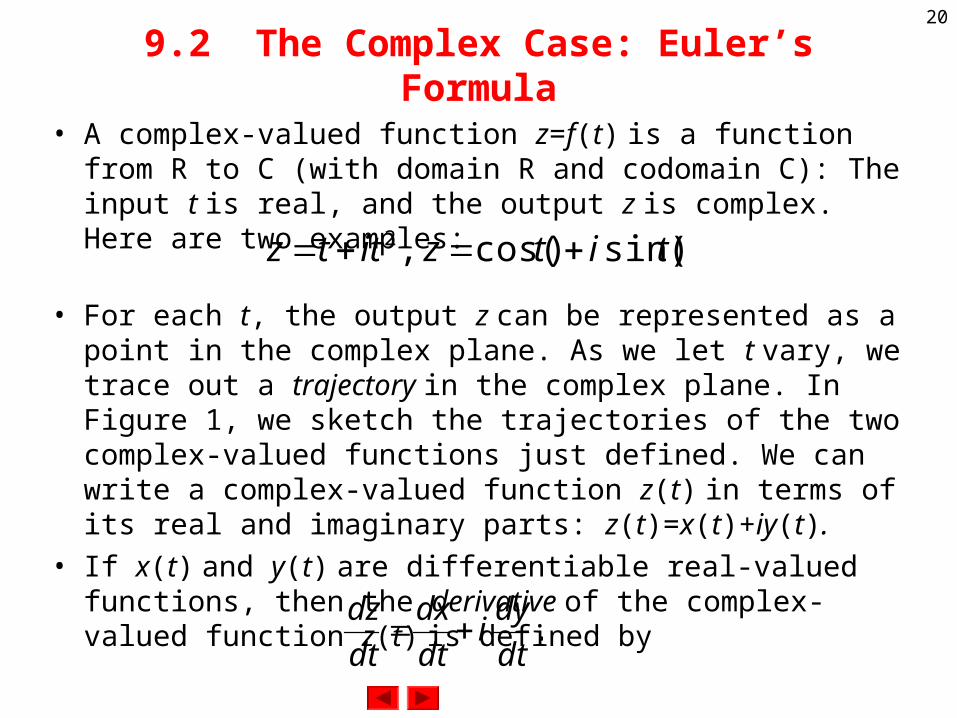
• A complex-valued function z=f(t) is a function from R to C (with domain R and codomain C): The input t is real, and the output z is complex. Here are two examples:

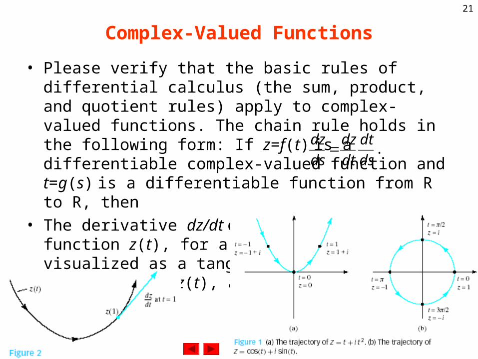
• For each t, the output z can be represented as a point in the complex plane. As we let t vary, we trace out a trajectory in the complex plane. In Figure 1, we sketch the trajectories of the two complex-valued functions just defined. We can write a complex-valued function z(t) in terms of its real and imaginary parts: z(t)=x(t)+iy(t).

• If x(t) and y(t) are differentiable real-valued functions, then the derivative of the complex-valued function z(t) is defined by

).sin()cos( ,2 titzittz

.dt

dyi

dt

dx

dt

dz

21

Complex-Valued Functions

• Please verify that the basic rules of differential calculus (the sum, product, and quotient rules) apply to complex-valued functions. The chain rule holds in the following form: If z=f(t) is a differentiable complex-valued function and t=g(s) is a differentiable function from R to R, then

• The derivative dz/dt of a complex-valued function z(t), for a given t, can be visualized as a tangent vector to the trajectory at z(t), as shown in Figure 2.

.ds

dt

dt

dz

ds

dz

22

Complex Exponential Functions

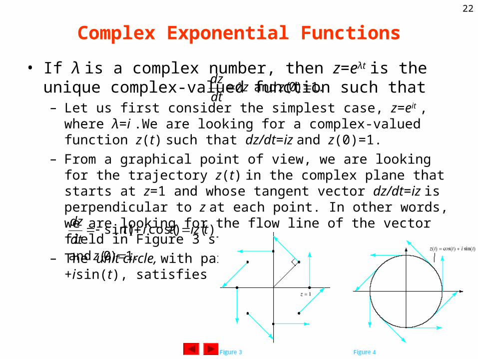
• If λ is a complex number, then z=eλt is the unique complex-valued function such that– Let us first consider the simplest case, z=eit , where λ=i .We are looking

for a complex-valued function z(t) such that dz/dt=iz and z(0)=1.

– From a graphical point of view, we are looking for the trajectory z(t) in the complex plane that starts at z=1 and whose tangent vector dz/dt=iz is perpendicular to z at each point. In other words, we are looking for the flow line of the vector field in Figure 3 starting at z=1.

– The unit circle, with parametrization z(t)=cos(t)+isin(t), satisfies

.1)0( and zzdt

dz

.1)0( and

)()cos()sin(

z

tiztitdt

dz

23

Euler’s Formula

• Euler’s formula: eit=cos(t)+isin(t).

• Euler’s formula can be used to write the polar form of a complex number more succinctly: z=r(cosφ+isinφ)=reiφ.

• Now consider z=eλt, where λ is an arbitrary complex number, λ=p+iq. By manipulating exponentials as if they were real, we find that eλt=e(p+iq)t=epteiqt=ept(cos(qt)+isin(qt)).

• We can validate this result by checking that the complex-valued function z(t)=ept(cos(qt)+isin(qt)) does indeed satisfy the definition of eλt , namely, dz/dt=λz and z(0)=1:

.))sin()(cos()(

))cos()sin(())sin()(cos(

zqtiqteiqp

qtiqqtqeqtiqtpedt

dz

pt

ptpt

24

Example 2

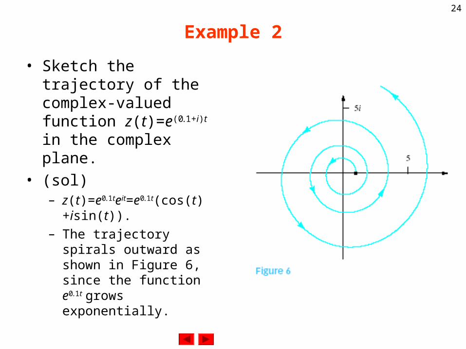
• Sketch the trajectory of the complex-valued function z(t)=e(0.1+i)t in the complex plane.

• (sol)– z(t)=e0.1teit=e0.1t(cos(t)+isin(t)).

– The trajectory spirals outward as shown in Figure 6, since the function e0.1t grows exponentially.

25

Example 3

• For which complex numbers λ is

• (sol)– Recall that z(t)=e0.1teit=e0.1t(cos(t)+isin(t)), so that |eλt|=ept. This quantity

approaches zero if (and only if) p is negative (i.e., if ept decays exponentially).

– We summarize: if (and only if) the real part of λ is negative.

?0lim

t

te

0lim

t

te

26

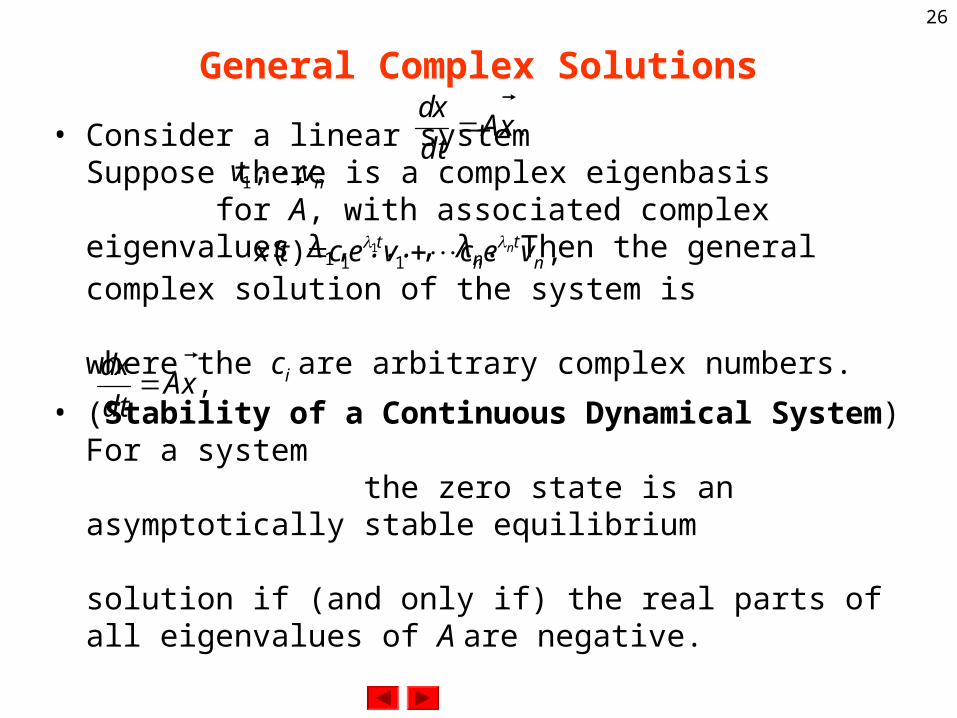
General Complex Solutions

• Consider a linear system Suppose there is a complex eigenbasis for A, with associated complex eigenvalues λ1, . . . , λn. Then the general complex solution of the system is

where the ci are arbitrary complex numbers.

• (Stability of a Continuous Dynamical System) For a system the zero state is an asymptotically stable equilibrium

solution if (and only if) the real parts of all eigenvalues of A are negative.

.xAdt

xd

nvv

,,1

,)( 111

nt

nt vecvectx n

,xAdt

xd

27

Example 4

• Consider the system where A is a (real) 2×2 matrix. When is the zero state a stable equilibrium solution for this system? Give your answer in terms of tr(A) and det(A).

• (sol)– We observe stability either if A has two negative eigenvalues or if A has

two conjugate eigenvalues p±iq, where p is negative. In both cases, tr(A) is negative and det(A) is positive. Check that in all other cases tr(A)≥0 or det(A)≤0.

,/ xAdtxd

28

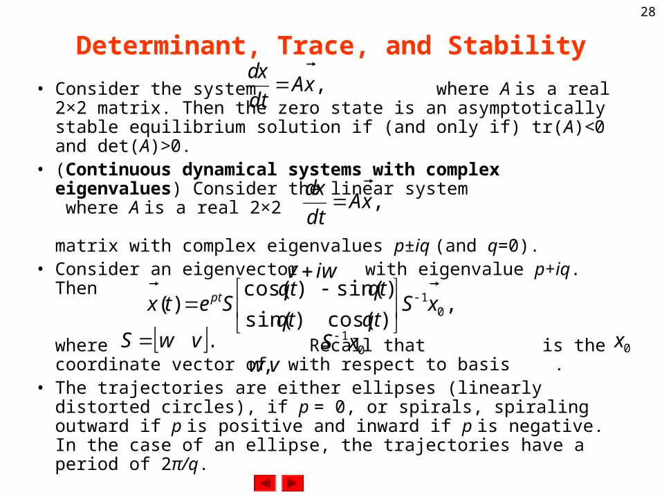
Determinant, Trace, and Stability

• Consider the system where A is a real 2×2 matrix. Then the zero state is an asymptotically stable equilibrium solution if (and only if) tr(A)<0 and det(A)>0.

• (Continuous dynamical systems with complex eigenvalues) Consider the linear system where A is a real 2×2

matrix with complex eigenvalues p±iq (and q=0).• Consider an eigenvector with eigenvalue p+iq. Then

where Recall that is the coordinate vector of with respect to basis .

• The trajectories are either ellipses (linearly distorted circles), if p = 0, or spirals, spiraling outward if p is positive and inward if p is negative. In the case of an ellipse, the trajectories have a period of 2π/q.

,xAdt

xd

,xAdt

xd

wiv

,)cos()sin(

)sin()cos()( 0

1xSqtqt

qtqtSetx pt

.vwS

0

1xS

0x

vw

,

29

Example 5

• Solve the system

• (sol)– The eigenvalues are λ1,2=±i , so that p=0 and q=1. This tells us that the

trajectory is an ellipse. To determine the direction of the trajectory (clockwise or counterclockwise) and its rough shape, we can draw the direction field for a few simple points , say, and , and sketch the flow line starting at See Figure 7.

– Now let us find a formula for the trajectory.

.1

0 with

35

230

xxdt

xd

xA

x

1ex

2ex

.1

0

wv

i

ii

ispan

i

iE

1

0

3

2

3

2

3

2

35

23ker

30

Example 5 (II)

– Therefore,

– You can check that

– The trajectory is the ellipse shown in Figure 8.

.3

2)sin(

1

0)cos(

)sin(3)cos(

)sin(2

0

1

)cos()sin(

)sin()cos(

31

20

)cos()sin(

)sin()cos()( 0

1

tttt

t

tt

ttxS

qtqt

qtqtSetx pt

.1

0)0( and

xxA

dt

xd

31

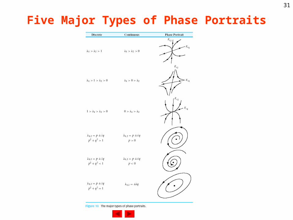
Five Major Types of Phase Portraits

32

9.3 Linear Differential Operators and Linear Differential Equation

• A transformation T from C∞ to C∞ of the form: T(f)=f(n)

+an-1f(n-1)+···+a1f1+a0fis called an nth-order linear differential operator. Here f(k) denotes the kth derivative of function f, and the coefficients ak are complex scalars.

• If T is an nth-order linear differential operator and g is a smooth function, then the equation T(f)=g or f(n)+an-

1f(n-1)+···+a1f1+a0f=g is called an nth-order linear differential equation (DE). The DE is called homogeneous if g = 0 and inhomogeneous otherwise.

33

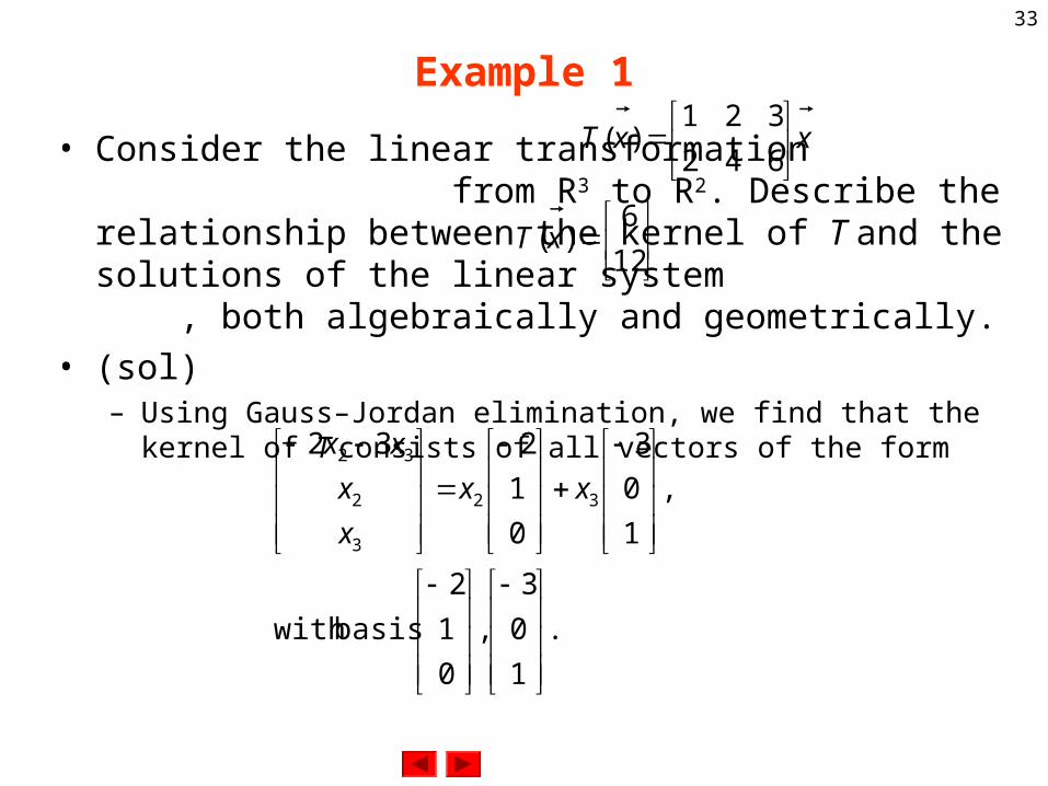
Example 1

• Consider the linear transformation from R3 to R2. Describe the relationship between the kernel of T and the solutions of the linear system , both algebraically and geometrically.

• (sol)– Using Gauss–Jordan elimination, we find that the kernel of T consists of

all vectors of the form

xxT

642

321)(

12

6)(xT

.

1

0

3

,

0

1

2

basiswith

,

1

0

3

0

1

232

32

3

2

32

xx

x

x

xx

34

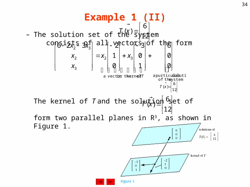
Example 1 (II)

– The solution set of the system consists of all vectors of the form

The kernel of T and the solution set of

form two parallel planes in R3, as shown in Figure 1.

12

6)(xT

12

6)(

system theofsolution purticular a of kernel in the vector a

32

3

2

32

0

0

6

1

0

3

0

1

2326

xT

T

xx

x

x

xx

12

6)(xT

35

nth-order Linear DE

• Consider a linear transformation T from V to W, where V and W are arbitrary linear spaces. Suppose we have a basis f1, f2,..., fn of the kernel of T . Consider an equation T( f ) = g with a particular solution f p. Then the solutions f of the equation T(f)=g are of the form f=c1f1+c2f2+···+cnfn+fp, where the ci are arbitrary constants.

• To solve an nth-order linear DE T(f)=g, we have to find– a basis f1,..., fn of kernel(T),– a particular solution fp of the DE.– Then the solutions f are of the form f=c1f1+···+cnfn+fp, where the ci

are arbitrary constants.

36

Example 2

• The kernel of an nth-order linear differential operator is n-dimensional.

• (Example 2) Find all solutions of the DE f’’(t)+f(t) = et. We are told that is a particular solution (verify this).

• (sol)– Consider the linear differential operator T(f) = f ‘’+f . A basis of the

kernel of T is f1(t)=cos(t) and f2(t) = sin(t).

– Therefore, the solutions f of the DE f’’+f=et are of the form.

tp etf 2

1)(

constants.arbitrary are and where,)sin()cos()( 2121

21 ccetctctf t

37

Eigenfunctions

• Consider a linear differential operator T from C∞ to C∞. A smooth function f is called an eigenfunction of T if T(f)=λf for some complex scalar λ; this scalar λ is called the eigenvalue associated with the eigenfunction f .

• (Example 3) Find all eigenfunctions and eigenvalues of the operator D(f)=f’.

• (sol)– We have to solve the differential equation f’=λf.– We know that for a given λ, the solutions are all exponential

functions of the form f(t)=Ceλt. This means that all complex numbers are eigenvalues of D, and the eigenspace associated with the eigenvalue λ is one-dimensional, spanned by eλt .

38

Characteristic Polynomial

• Consider the linear differential operatorT(f)=f(n)+an-1f(n-1)+···+a1f1+a0fThe characteristic polynomial of T is defined aspT(λ)=λn+an-1λn-1+···+a1λ+a0.

• If T is a linear differential operator, then eλt is an eigenfunction of T , with associated eigenvalue pT(λ), for all λ: T(eλt)=pT(λ)eλt. In particular, if pT(λ)=0, then eλt is in the kernel of T.

39

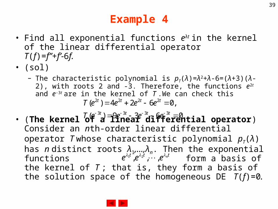
Example 4

• Find all exponential functions eλt in the kernel of the linear differential operatorT(f)=f’’+f’-6f.

• (sol)– The characteristic polynomial is pT(λ)=λ2+λ-6=(λ+3)(λ-2), with roots 2

and -3. Therefore, the functions e2t and e-3t are in the kernel of T .We can check this

• (The kernel of a linear differential operator)Consider an nth-order linear differential operator T whose characteristic polynomial pT(λ) has n distinct roots λ1,...,λn. Then the exponential functions form a basis of the kernel of T ; that is, they form a basis of the solution space of the homogeneous DE T(f)=0.

.0639)(

,0624)(3333

2222

tttt

tttt

eeeeT

eeeeT

ttt neee ,,, 21

40

Example 5

• Find all solutions f of the differential equationf‘’+2f’-3f=0.

• (sol)– The characteristic polynomial of the operator T(f)=f’’+2f’-3f is

pT(λ)=λ2+2λ-3=(λ+3)(λ-1), with roots 1 and .3. The exponential functions et and e-3t form a basis of the solution space, i.e., the solutions are of the form f(t)=c1et+c2e-3t .

41

Example 6• Find all solutions f of the differential equation

f’’-6f+13f = 0.

• (sol)– The characteristic polynomial is pT(λ)=λ2-6λ+13, with complex roots

3±2i. The exponential functions

– form a basis of the solution space.We may wish to find a basis of the solution space consisting of real-valued functions. The following observation is helpful: if f(t)=g(t)+ih(t) is a solution of the DE T(f)=0, then T(f)=T(g)+iT(h)=0, so that g and h are solutions as well. We can apply this remark to the real and the imaginary parts of the solution e(3+2i)t : The functions e3tcos(2t) and e3t sin(2t) are a basis of the solution space (they are clearly linearly independent), and the general solution isf(t)=c1e3tcos(2t)+c2e3tsin(2t)=e3t(c1cos(2t)+c2sin(2t)).

))2sin()2(cos(

and ))2sin()2(cos(3)23(

3)23(

titee

titeetti

tti

42

The solutions of the DE• Consider a differential equation T(f)=f’’+af’+bf=0, where the

coefficients a and b are real. Suppose the zeros of pT(λ) are p±iq, with q=0. Then the solutions of the given DE are f(t)=ept(c1cos(qt)+c2sin(qt)), where c1 and c2 are arbitrary constants.The special case when a=0 and b>0 is important in many applications. Then p=0 and q = , so that the solutions of the DE f‘’+bf= 0 are

• Note that the functionf(t)=ept(c1cos(qt)+c2sin(qt))is the product of an exponentialand a sinusoidal function. The case when p is negative comesup frequently in physics, whenwe model a damped oscillator.See Figure 2.

b

).sin()cos()( 21 tbctbctf

43

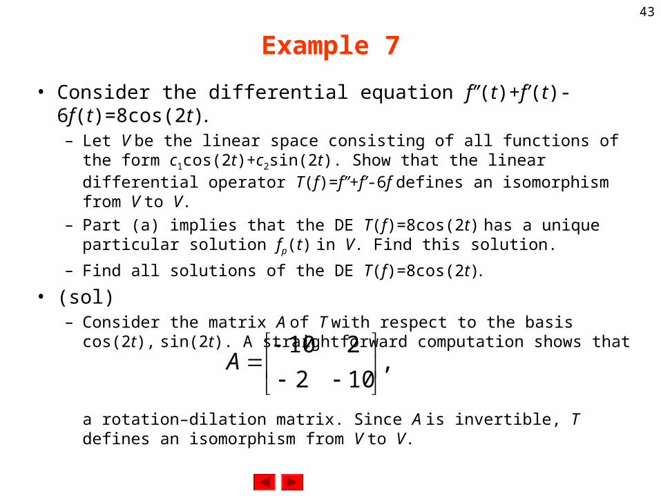
Example 7

• Consider the differential equation f’’(t)+f’(t)-6f(t)=8cos(2t).– Let V be the linear space consisting of all functions of the form c1cos(2t)

+c2sin(2t). Show that the linear differential operator T(f)=f”+f’-6f defines an isomorphism from V to V.

– Part (a) implies that the DE T(f)=8cos(2t) has a unique particular solution fp(t) in V. Find this solution.

– Find all solutions of the DE T(f)=8cos(2t).

• (sol)– Consider the matrix A of T with respect to the basis cos(2t), sin(2t). A

straightforward computation shows that

a rotation–dilation matrix. Since A is invertible, T defines an isomorphism from V to V.

,102

210

A

44

Example 7 (II)

– If we work in coordinates with respect to the basis cos(2t), sin(2t), the DE T(f)=8cos(2t) takes the form with the solution

The particular solution in V is

A more straightforward way to find fp(t) is to set fp(t)=Pcos(2t)+Qsin(2t) and substitute this trial solution into the DE to determine P and Q.

– The solutions of the DE are of the form

,0

8

xA

.13/2

13/10

0

8

102

210

104

1

0

81

Ax

).2sin(13

2)2cos(

13

10)( tttf p

).2sin(13

2)2cos(

13

10

)()()()(

32

21

2211

ttecec

tftfctfctf

tt

p

45

A Particular Solution of the DE

• Consider the linear differential equation f”(t)+af’(t)+bf(t)=Ccos(ωt), where a, b, C, and ω are real numbers. Suppose that a≠0 or b≠ω2. This DE has a particular solution of the form fp(t)=Pcos(ωt)+Qsin(ωt).

• An nth-order linear differential operator T can be expressed as the composite of n first-order linear differential operators:T=Dn+an-1Dn-1+···+a1D+a0=(D-λ1)(D-λ2)...(D-λn), where the λi are complex numbers.

46

Example 8

• Find the kernel of the operator T=D-a, where a is a complex number.

• (sol)– We have to solve the homogeneous differential equation T(f)=0 or f’(t)-

af(t)=0 or f’(t)=af(t). By definition of an exponential function, the solutions are the functions of the form f(t)=Ceat, where C is an arbitrary constant.

• The kernel of the operator T=D-a is one-dimensional, spanned by f(t)=eat.

• Consider the differential equation f’(t)-af(t)=g(t), where g(t) is a smooth function and a a constant. Then

.)()( dttgeetf atat

47

Example 9• Find the solutions f of the DE f’-af=ceat, where c is an arbitrary

constant.• (sol)

– We find thatwhere C is another arbitrary constant.

– Now consider an nth-order DE T(f)=g, where T=Dn+an-1Dn-1+···+a1D+a0=(D-λ1)(D-λ2)...(D-λn-1)(D-λn).

– We can break this DE down into n first-order DEs:

– We can successively solve the first-order DEs:(D-λ1)f1=g,(D-λ2)f2=g, :(D-λn-1)fn-1=g,(D-λn)fn=g,

– In particular, the DE T(f)=g does have solutions f .

),()( Cctecdtedtceeetf atatatatat

48

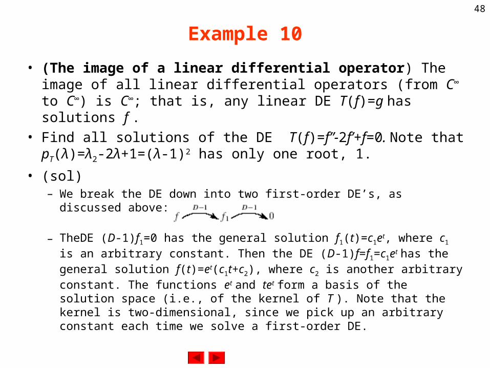
Example 10

• (The image of a linear differential operator) The image of all linear differential operators (from C∞ to C∞) is C∞; that is, any linear DE T(f)=g has solutions f .

• Find all solutions of the DE T(f)=f”-2f’+f=0. Note that pT(λ)=λ2-2λ+1=(λ-1)2 has only one root, 1.

• (sol)– We break the DE down into two first-order DE’s, as discussed above:

– TheDE (D-1)f1=0 has the general solution f1(t)=c1et, where c1 is an arbitrary constant. Then the DE (D-1)f=f1=c1et has the general solution f(t)=et(c1t+c2), where c2 is another arbitrary constant. The functions et and tet form a basis of the solution space (i.e., of the kernel of T ). Note that the kernel is two-dimensional, since we pick up an arbitrary constant each time we solve a first-order DE.

49

Strategy for Linear Differential Equations

• Suppose you have to solve an nth-order linear differential equation T(f)=g.– (Step 1) Find n linearly independent solutions of the DE T(f)=0.

• Write the characteristic polynomial pT(λ) of T(replacing f(k) by λk).

• Find the solutions λ1, λ2,..., λn of the equation pT(λ)=0.

• If λ is a solution of the equation pT(λ)=0, then eλt is a solution of T(f)=0.

• If λ is a solution of pT(λ)=0 with multiplicity m, then eλt, teλt, t2eλt,..., tm-1eλt are solutions of the DE T(f)=0.

• If p ±iq are complex solutions of pT(λ)=0, then eptcos(qt) and eptsin(qt) are real solutions of the DE T(f)=0.

50

Strategy for Linear Differential Equations (II)

– (Step 2) If the DE is inhomogeneous (i.e., if g=0), find one particular solution fp of the DE T(f)=g.

• If g is of the form g(t)=Acos(ωt)+Bsin(ωt), look for a particular solution of the same form, fp(t)=Pcos(ωt)+Qsin(ωt).

• If g is constant, look for a constant particular solution fp(t)=c.

• If the DE is of first order, of the form f’(t)-af(t)=g(t), use the formula

• If none of the preceding techniques applies, write T=(D-λ1)(D-λ2)···(D-λn), and solve the corresponding first order DEs.

– (Step 3) The solutions of the DE T(f)=g are of the form f(t)=c1f1(t)+c2f2(t)+···+cnfn(t)+fp(t), where f1, f2,..., fn are the solutions from step 1 and fp is the solution from step 2.

.)()( dttgeetf atat

51

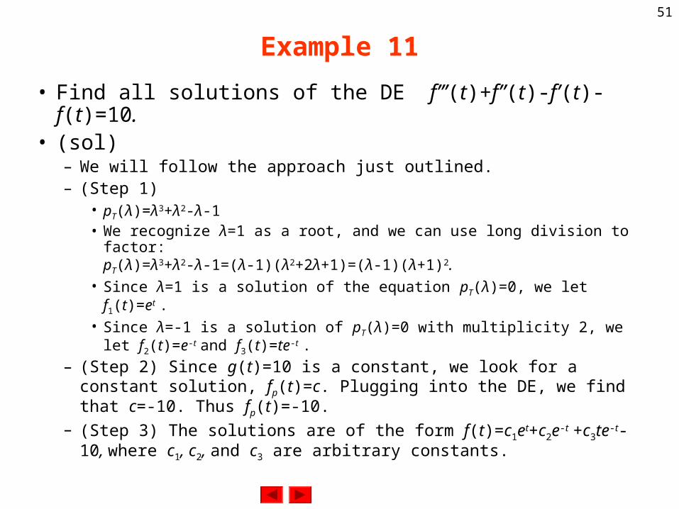
Example 11

• Find all solutions of the DE f’’’(t)+f”(t)-f’(t)-f(t)=10.• (sol)

– We will follow the approach just outlined.– (Step 1)

• pT(λ)=λ3+λ2-λ-1• We recognize λ=1 as a root, and we can use long division to factor:

pT(λ)=λ3+λ2-λ-1=(λ-1)(λ2+2λ+1)=(λ-1)(λ+1)2.• Since λ=1 is a solution of the equation pT(λ)=0, we let f1(t)=et .• Since λ=-1 is a solution of pT(λ)=0 with multiplicity 2, we let f2(t)=e-t

and f3(t)=te-t .

– (Step 2) Since g(t)=10 is a constant, we look for a constant solution, fp(t)=c. Plugging into the DE, we find that c=-10. Thus fp(t)=-10.

– (Step 3) The solutions are of the form f(t)=c1et+c2e-t +c3te-t-10, where c1, c2, and c3 are arbitrary constants.