Basic theory of the gamma function derived from Euler’s limit definition

Notes by G.J.O. Jameson

Contents

1. Euler’s limit, and the associated product and series expressions

2. Elementary applications

3. Three identities

4. The power series for ψ(z) and log Γ(z)

5. Alternative proof of convergence in the real case

6. Inequalities for gamma function ratios; the Bohr-Mollerup theorem

7. Equivalence with the integral definition

1. Euler’s limit, and the associated product and series expressions

Euler’s integral definition of the gamma function, valid for Re z > 0, is Γ(z) =∫∞0tz−1e−t dt. In 1729, Euler developed another definition of the gamma function as the

limit of a certain expression. To motivate this expression, observe that for positive integers

k and n,

(k − 1)! =(n+ k)!

k(k + 1) . . . (n+ k)

and(n+ k)!

nkn!=

(n+ 1)(n+ 2) . . . (n+ k)

nk=

(1 +

1

n

) (1 +

2

n

). . .

(1 +

k

n

).

Denote this by C(n, k). Then C(n, k) → 1 as n→∞ and (k − 1)! = C(n, k)Γn(k), where

Γn(k) =nkn!

k(k + 1) . . . (k + n).

So we have shown that limn→∞ Γn(k) = (k − 1)!.

Now define, for complex z other than 0 and negative real integers,

Γn(z) =nzn!

z(z + 1) . . . (z + n),

where nz means ez log n. We will show that limn→∞ Γn(z) actually exists for all complex z

except 0 and negative integers (a pleasant alternative proof for the real case is given in

section 5). This is Euler’s limit definition of the gamma function. Here we will show how

to derive the basic properties of the gamma function from this definition. Some of them

can be proved equally easily from the integral definition, but others cannot. In particular,

Euler’s limit equates to certain infinite product expressions, which are sometimes adopted as

1

yet another equivalent definition. These expressions, or their logarithmic equivalent, imply

differentiability, together with a series expression, not for Γ′(z) itself, but for Γ′(z)/Γ(z).

This, in turn, leads to numerous further identities and estimations.

Ultimately, a full understanding of the gamma function requires a judicious combina-

tion of both definitions. Equivalence of the two definitions is proved in section 7, but this

section does not depend on the earlier ones, and could be read first.

Most of the methods presented here are standard, e.g. see [Cop, chapter 9]. The

methods described in sections 5 and 6 are less well known; they have appeared in my articles

[Jam1], [Jam2].

We will actually work with the following slight variant of Euler’s limit: let

Gn(z) =nz(n− 1)!

z(z + 1) . . . (z + n− 1). (1)

The numerator nz(n− 1)! can equally be written as nz−1n!. Clearly,

Γn(z) =n

z + nGn(z),

which shows that convergence of either implies convergence of the other, with the same limit.

Note that Gn(1) = 1, while Γn(1) = n/(n+1), which suggests that in some sense Gn is more

“natural” than Γn. We observe also that

Gn(z + 1) =nz

n+ zGn(z),

so once we have established convergence, the functional equation Γ(z+1) = zΓ(z) will follow

immediately. (This will establish again that Γ(n) = (n − 1)!.) Note also that Gn(z + 1) =

zΓn(z).

We will work with logGn(z). For positive, real z, this presents no problem, and the

following proofs become simpler in places. In the complex case, we need to take some care

over logarithms. Any w such that ew = z is called a logarithm of z. For all z 6= 0, we

can express z as reiθ with −π < θ ≤ π, and the principal logarithm of z, which we denote

by log z, is log r + iθ. (Note that this applies to negative real x, with θ = −π.) Write

R− = {x ∈ R : x ≤ 0}. The following properties apply:

(L1) For positive real x, log(z/x) = log z − log x.

(L2) For z ∈ C \ R−, log z =∫

[1,z]1ζdζ, where [1, z] is the straight-line path from 1 to z.

(L3) For z ∈ C \ R−, log z is differentiable, with derivative 1/z.

(L4) log(1 + z) =∑∞

n=1(−1)n−1zn/n for all z with |z| < 1.

(L5) by (L4), we have | log(1 + z)− z| ≤ |z|2 for |z| ≤ 12.

2

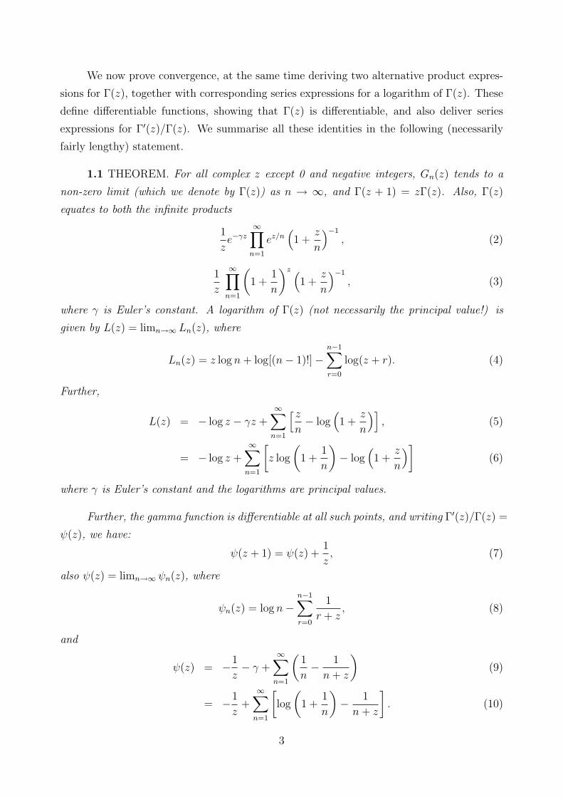
We now prove convergence, at the same time deriving two alternative product expres-

sions for Γ(z), together with corresponding series expressions for a logarithm of Γ(z). These

define differentiable functions, showing that Γ(z) is differentiable, and also deliver series

expressions for Γ′(z)/Γ(z). We summarise all these identities in the following (necessarily

fairly lengthy) statement.

1.1 THEOREM. For all complex z except 0 and negative integers, Gn(z) tends to a

non-zero limit (which we denote by Γ(z)) as n → ∞, and Γ(z + 1) = zΓ(z). Also, Γ(z)

equates to both the infinite products

1

ze−γz

∞∏n=1

ez/n(1 +

z

n

)−1

, (2)

1

z

∞∏n=1

(1 +

1

n

)z (1 +

z

n

)−1

, (3)

where γ is Euler’s constant. A logarithm of Γ(z) (not necessarily the principal value!) is

given by L(z) = limn→∞ Ln(z), where

Ln(z) = z log n+ log[(n− 1)!]−n−1∑r=0

log(z + r). (4)

Further,

L(z) = − log z − γz +∞∑

n=1

[ zn− log

(1 +

z

n

)], (5)

= − log z +∞∑

n=1

[z log

(1 +

1

n

)− log

(1 +

z

n

)](6)

where γ is Euler’s constant and the logarithms are principal values.

Further, the gamma function is differentiable at all such points, and writing Γ′(z)/Γ(z) =

ψ(z), we have:

ψ(z + 1) = ψ(z) +1

z, (7)

also ψ(z) = limn→∞ ψn(z), where

ψn(z) = log n−n−1∑r=0

1

r + z, (8)

and

ψ(z) = −1

z− γ +

∞∑n=1

(1

n− 1

n+ z

)(9)

= −1

z+

∞∑n=1

[log

(1 +

1

n

)− 1

n+ z

]. (10)

3

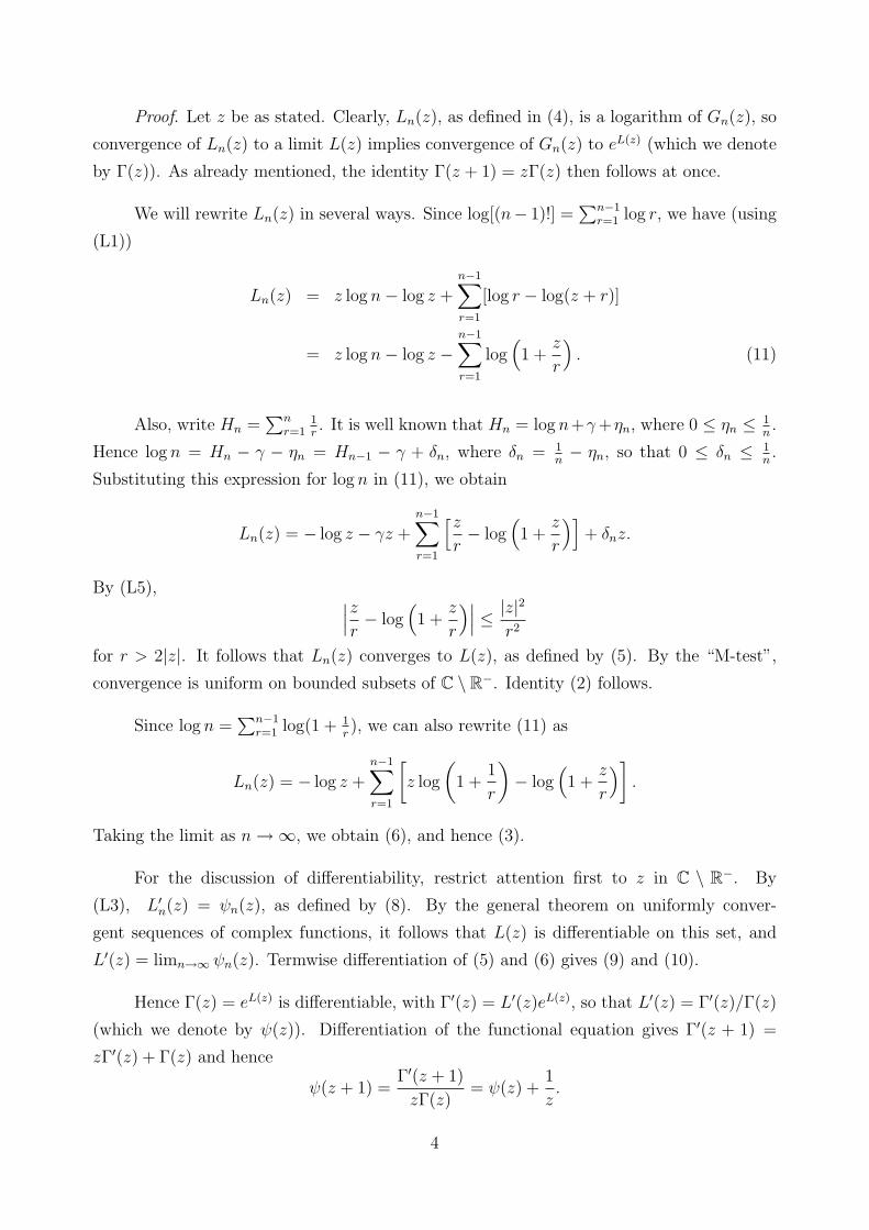
Proof. Let z be as stated. Clearly, Ln(z), as defined in (4), is a logarithm of Gn(z), so

convergence of Ln(z) to a limit L(z) implies convergence of Gn(z) to eL(z) (which we denote

by Γ(z)). As already mentioned, the identity Γ(z + 1) = zΓ(z) then follows at once.

We will rewrite Ln(z) in several ways. Since log[(n− 1)!] =∑n−1

r=1 log r, we have (using

(L1))

Ln(z) = z log n− log z +n−1∑r=1

[log r − log(z + r)]

= z log n− log z −n−1∑r=1

log(1 +

z

r

). (11)

Also, write Hn =∑n

r=11r. It is well known that Hn = log n+γ+ηn, where 0 ≤ ηn ≤ 1

n.

Hence log n = Hn − γ − ηn = Hn−1 − γ + δn, where δn = 1n− ηn, so that 0 ≤ δn ≤ 1

n.

Substituting this expression for log n in (11), we obtain

Ln(z) = − log z − γz +n−1∑r=1

[zr− log

(1 +

z

r

)]+ δnz.

By (L5), ∣∣∣zr− log

(1 +

z

r

)∣∣∣ ≤ |z|2

r2

for r > 2|z|. It follows that Ln(z) converges to L(z), as defined by (5). By the “M-test”,

convergence is uniform on bounded subsets of C \ R−. Identity (2) follows.

Since log n =∑n−1

r=1 log(1 + 1r), we can also rewrite (11) as

Ln(z) = − log z +n−1∑r=1

[z log

(1 +

1

r

)− log

(1 +

z

r

)].

Taking the limit as n→∞, we obtain (6), and hence (3).

For the discussion of differentiability, restrict attention first to z in C \ R−. By

(L3), L′n(z) = ψn(z), as defined by (8). By the general theorem on uniformly conver-

gent sequences of complex functions, it follows that L(z) is differentiable on this set, and

L′(z) = limn→∞ ψn(z). Termwise differentiation of (5) and (6) gives (9) and (10).

Hence Γ(z) = eL(z) is differentiable, with Γ′(z) = L′(z)eL(z), so that L′(z) = Γ′(z)/Γ(z)

(which we denote by ψ(z)). Differentiation of the functional equation gives Γ′(z + 1) =

zΓ′(z) + Γ(z) and hence

ψ(z + 1) =Γ′(z + 1)

zΓ(z)= ψ(z) +

1

z.

4

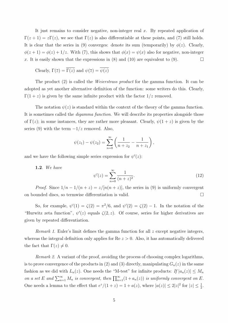
It just remains to consider negative, non-integer real x. By repeated application of

Γ(z + 1) = zΓ(z), we see that Γ(z) is also differentiable at these points, and (7) still holds.

It is clear that the series in (9) converges: denote its sum (temporarily) by φ(z). Clearly,

φ(z + 1) = φ(z) + 1/z. With (7), this shows that φ(x) = ψ(x) also for negative, non-integer

x. It is easily shown that the expressions in (8) and (10) are equivalent to (9). �

Clearly, Γ(z) = Γ(z) and ψ(z) = ψ(z)

The product (2) is called the Weierstrass product for the gamma function. It can be

adopted as yet another alternative definition of the function: some writers do this. Clearly,

Γ(1 + z) is given by the same infinite product with the factor 1/z removed.

The notation ψ(z) is standard within the context of the theory of the gamma function.

It is sometimes called the digamma function. We will describe its properties alongside those

of Γ(z); in some instances, they are rather more pleasant. Clearly, ψ(1 + z) is given by the

series (9) with the term −1/z removed. Also,

ψ(z1)− ψ(z2) =∞∑

n=0

(1

n+ z2

− 1

n+ z1

),

and we have the following simple series expression for ψ′(z):

1.2. We have

ψ′(z) =∞∑

n=0

1

(n+ z)2. (12)

Proof. Since 1/n− 1/(n + z) = z/[n(n + z)], the series in (9) is uniformly convergent

on bounded discs, so termwise differentiation is valid. �

So, for example, ψ′(1) = ζ(2) = π2/6, and ψ′(2) = ζ(2) − 1. In the notation of the

“Hurwitz zeta function”, ψ′(z) equals ζ(2, z). Of course, series for higher derivatives are

given by repeated differentiation.

Remark 1. Euler’s limit defines the gamma function for all z except negative integers,

whereas the integral definition only applies for Re z > 0. Also, it has automatically delivered

the fact that Γ(z) 6= 0.

Remark 2. A variant of the proof, avoiding the process of choosing complex logarithms,

is to prove convergence of the products in (2) and (3) directly, manipulatingGn(z) in the same

fashion as we did with Ln(z). One needs the “M-test” for infinite products: If |an(z)| ≤Mn

on a set E and∑∞

n=1Mn is convergent, then∏∞

n=1(1+an(z)) is uniformly convergent on E.

One needs a lemma to the effect that ez/(1 + z) = 1 + a(z), where |a(z)| ≤ 2|z|2 for |z| ≤ 12.

5

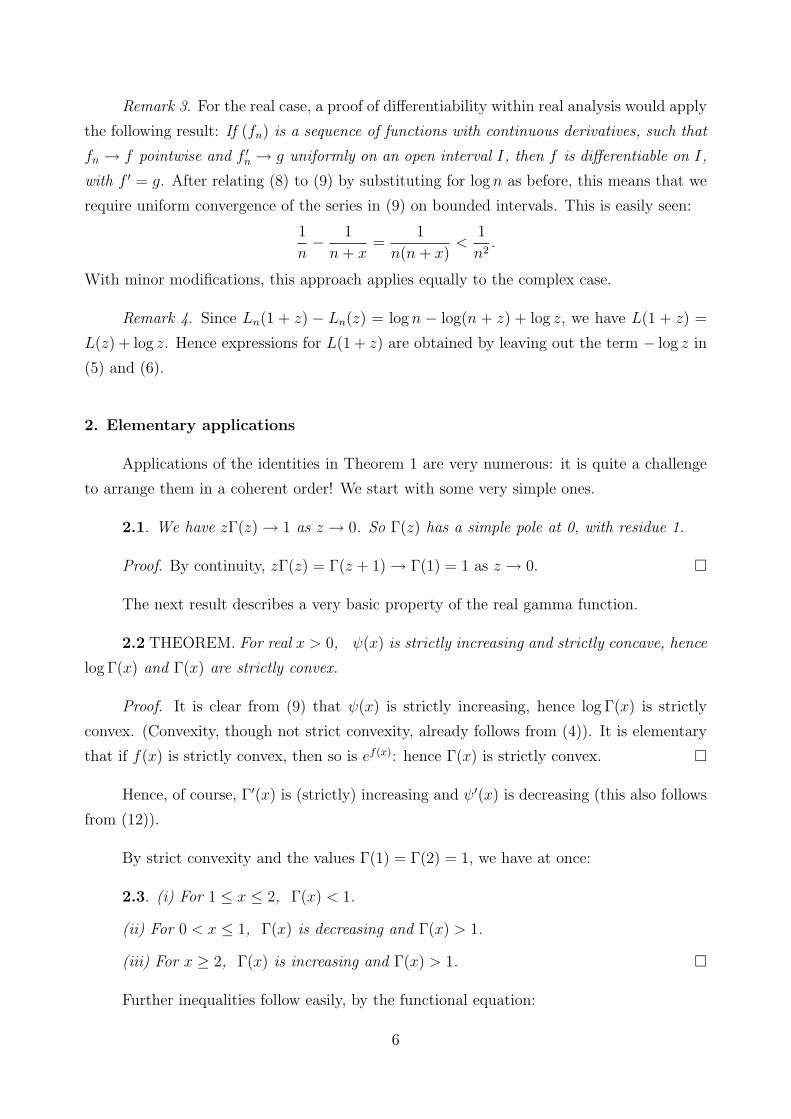
Remark 3. For the real case, a proof of differentiability within real analysis would apply

the following result: If (fn) is a sequence of functions with continuous derivatives, such that

fn → f pointwise and f ′n → g uniformly on an open interval I, then f is differentiable on I,

with f ′ = g. After relating (8) to (9) by substituting for log n as before, this means that we

require uniform convergence of the series in (9) on bounded intervals. This is easily seen:

1

n− 1

n+ x=

1

n(n+ x)<

1

n2.

With minor modifications, this approach applies equally to the complex case.

Remark 4. Since Ln(1 + z) − Ln(z) = log n − log(n + z) + log z, we have L(1 + z) =

L(z) + log z. Hence expressions for L(1 + z) are obtained by leaving out the term − log z in

(5) and (6).

2. Elementary applications

Applications of the identities in Theorem 1 are very numerous: it is quite a challenge

to arrange them in a coherent order! We start with some very simple ones.

2.1. We have zΓ(z) → 1 as z → 0. So Γ(z) has a simple pole at 0, with residue 1.

Proof. By continuity, zΓ(z) = Γ(z + 1) → Γ(1) = 1 as z → 0. �

The next result describes a very basic property of the real gamma function.

2.2 THEOREM. For real x > 0, ψ(x) is strictly increasing and strictly concave, hence

log Γ(x) and Γ(x) are strictly convex.

Proof. It is clear from (9) that ψ(x) is strictly increasing, hence log Γ(x) is strictly

convex. (Convexity, though not strict convexity, already follows from (4)). It is elementary

that if f(x) is strictly convex, then so is ef(x): hence Γ(x) is strictly convex. �

Hence, of course, Γ′(x) is (strictly) increasing and ψ′(x) is decreasing (this also follows

from (12)).

By strict convexity and the values Γ(1) = Γ(2) = 1, we have at once:

2.3. (i) For 1 ≤ x ≤ 2, Γ(x) < 1.

(ii) For 0 < x ≤ 1, Γ(x) is decreasing and Γ(x) > 1.

(iii) For x ≥ 2, Γ(x) is increasing and Γ(x) > 1. �

Further inequalities follow easily, by the functional equation:

6

2.4. (i) For 0 < x < 1, Γ(x) < 1/x.

(ii) For 1 < x < 2, Γ(x) > max(1/x, x− 1).

Proof. (i) Then xΓ(x) = Γ(1 + x) < 1.

(ii) Then 1 + x > 2, so xΓ(x) = Γ(1 + x) > 1. Also, 0 < x − 1 < 1, so Γ(x − 1) > 1,

hence Γ(x) = (x− 1)Γ(x− 1) > x− 1. �

Clearly, Γ(x) attains its least value at a point x0 in (1, 2): this is the point where

ψ(x0) = 0. By (ii), the least value is not less than the common value of 1/x and x − 1

where these intersect, i.e. 12(√

5 + 1) ≈ 0.618. In fact, it is known that x0 ≈ 1.4616, with

Γ(x0) ≈ 0.8856.

Example. A typical application of convexity of log Γ(x) is: log Γ(a+x)+log Γ(a−x) ≥2 log Γ(a) for 0 < x < a, hence Γ(a+x)Γ(a−x) ≥ Γ(a)2. In particular, Γ(1+x)Γ(1−x) ≥ 1

and Γ(2 + x)Γ(2 − x) ≥ 1 for 0 ≤ x ≤ 1. (We shall see later that there is an explicit

expression for these products.)

The next result describes the behaviour of Γ(z) on vertical lines.

2.5. For z = x + iy, we have |Γ(z)| ≤ |Γ(x)|. Also, |Γ(x + iy)| decreases with y for

y > 0, and |Γ(x+ iy)| ≤ |Γ(x+ 1)|/y, so Γ(x+ iy) → 0 as y →∞.

Proof. We have |nz| = nx and |z + r| ≥ |x + r|, so |Gn(z)| ≤ |Gn(x)|. Also, |z + r| =

|x+ r + iy| increases with y, so |Gn(z)| decreases with y. Further,

|Γ(x+ iy)| = |Γ(x+ 1 + iy)||x+ iy|

≤ |Γ(x+ 1)|y

.

(By considering x+ k + iy, one can show that |Γ(x+ iy| = O(y−k).) �

We now identify the values of ψ and Γ′ at positive integers.

2.6 PROPOSITION. We have ψ(1) = Γ′(1) = −γ.

Proof. In (8), we have ψn(1) = log n−Hn−1 → γ as n→∞. �

Recall the notation Hn =∑n

r=11r. By (7), we now deduce further:

2.7. We have ψ(2) = Γ′(2) = 1− γ, and for integers n ≥ 2, ψ(n) = Hn−1 − γ. �

Example. ψ(3) = 32− γ, hence Γ′(3) = 3− 2γ. Also, ψ(4) = 11

6− γ, so Γ′(4) = 11− 6γ.

We can now strengthen 2.1:

7

2.8. We have Γ(z)− 1/z → −γ as z → 0.

Proof. By 2.6, we have

Γ(z)− 1

z=

1

z

(Γ(1 + z)− 1

)→ Γ′(1) = −γ as z → 0. �

We can deduce the following further inequalities, using the fact that convex functions

lie above their tangents, together with the values at 1 and 2:

2.9. For 0 < x < 1, we have:

(i) log Γ(1 + x) ≥ −γx, hence Γ(1 + x) ≥ e−γx;

(ii) Γ(1 + x) ≥ 1− γx, so 1/x− γ ≤ Γ(x) < 1/x;

(iii) Γ(1 + x) ≥ γ + (1− γ)x. �

The two lower bounds for Γ(1+x) in 2.9 intersect at x = 1−γ, improving our previous

estimate for the minimum value Γ(x0) to 1− γ + γ2 ≈ 0.7559.

We now state some corresponding results for ψ(z):

2.10. When z → 0, we have zψ(z) → −1, ψ(z) + 1/z → −γ and z2Γ′(z) → −1. For

real x with 0 ≤ x ≤ 1, we have ψ(1 + x) = ψ(x) + 1/x ≥ x− γ.

Proof. By continuity, ψ(z)+1/z = ψ(1+z) → ψ(1) = −γ as z → 0. Hence zψ(z) → −1.

With 2.1, this gives z2Γ′(z) = zΓ(z). zψ(z) → −1. Since ψ is concave, ψ(1) = −γ and

ψ(2) = 1− γ, we have ψ(1 + x) ≥ x− γ for real x in [0, 1]. �

Assuming, for the moment, equivalence with the integral definition of the gamma

function, we can deduce the “exponential integral”, direct evaluation of which is not entirely

trivial (e.g. see [Jam4]):

2.11 PROPOSITION. We have∫ ∞

0

e−t log t dt = −γ.

Proof. By the integral definition, Γ′(1) equates to this integral. �

Example. Recall from 1.2 that ψ′(1) = ζ(2). Now clearly

ψ′(z) =Γ′′(z)

Γ(z)− Γ′(z)2

Γ(z)2.

Hence Γ′′(1) = ψ′(1) + Γ′(1)2 = ζ(2) + γ2.

8

One can deduce further inequalities from the concavity of ψ, for example ψ(n + x) ≥Hn−1 − γ + x

nfor 0 ≤ x ≤ 1 and (from the tangent at 1) ψ(1 + x) ≤ ζ(2)x− γ for all x > 0.

However, a more pleasant estimation is obtained, in elegant style, as follows:

2.12 PROPOSITION. For all x > 0,

log x− 1

x≤ ψ(x) ≤ log x. (13)

Proof. We have log Γ(x + 1) − log Γ(x) = log x. But by the mean-value theorem,

log Γ(x+ 1)− log Γ(x) = ψ(ξ) for some ξ in (x, x+ 1). Since ψ is increasing, ψ(x) ≤ log x <

ψ(x+1). Since ψ(x+1) = ψ(x)+ 1x, this equates to (13). (Also, ψ(x) ≥ log(x− 1), but this

is weaker than (13).) �

By integration, we obtain corresponding inequalities for Γ(x).

2.13 COROLLARY. For all x > 0,

xx−1e1−x ≤ Γ(x) ≤ xxe1−x. (14)

Proof. Note that∫ x

1ψ(t) dt = log Γ(x). So, integration of (13) on [1, x] gives

(x− 1) log x− x+ 1 ≤ log Γ(x) ≤ x log x− x+ 1,

which equates to (14). �

The estimations in (13) and (14) can be greatly improved: the outcome is Stirling’s

formula. A simple exposition is given in [Jam3].

A similar proof shows that ψ′(x) is like 1/x for large x:

2.14. For all x > 0,1

x≤ ψ′(x) ≤ 1

x+

1

x2,

hence ψ(x)− log x is increasing and ψ(x)− log x+ 1/x is decreasing.

Proof. By the mean-value theorem, 1x

= ψ(x+1)−ψ(x) = ψ′(ξ) for some ξ in (x, x+1).

Since ψ′ is decreasing, ψ′(x) ≥ 1x≥ ψ′(x+ 1). Also, ψ′(x+ 1) = ψ′(x)− 1/x2. �

Alternatively, 2.14 can be proved by integral estimation of the series (12) for ψ′(x).

By the functional equation, we have

Γ(n+ z + 1) = z(z + 1) . . . (z + n)Γ(z).

9

We describe several consequences of this. First, Γ(x) has alternate signs on the intervals

between negative integers. In fact, if x ∈ (−n − 1,−n), then x + n < 0 < x + n + 1, so

(−1)n+1Γ(x) > 0. Also, we can deduce the nature of Γ(z) at integers −n:

2.15. For positive integers n, we have limz→−n(z + n)Γ(z) = (−1)n/n!, so Γ(z) has a

simple pole at −n, with residue (−1)n/n!.

Proof. We have

(z + n)Γ(z) =Γ(z + n+ 1)

z(z + 1) . . . (z + n− 1)→ Γ(1)

(−n) . . . (−2)(−1)=

(−1)n

n!as z → −n. �

2.16. For fixed z, we have Γ(n+ z) ∼ nz−1n! as n→∞.

Proof. By the definition (1) of Gn(z),

Gn(z) = nz−1n!Γ(z)

Γ(n+ z),

so Γ(n+ z) = nz−1n!Γ(z)/Gn(z). The statement follows. �

Similarly, we have for ψ(z):

2.17. For positive integers n, ψ(z) has a simple pole at −n, and ψ(−n+ z) + 1/z →Hn − γ as z → 0.

Proof. This follows from the fact that

ψ(−n+ z) = ψ(z) +1

1− z+

1

2− z+ · · ·+ 1

n− z,

together with 2.10. �

It follows that ψ(x) strictly increases from −∞ to ∞ on each interval (−n,−n+ 1).

Next, we establish the values of Γ(12) and ψ(1

2). We assume the Wallis product, which

can be stated as follows: let

Wn =2.4. . . . (2n)

1.3.5. . . . (2n− 1)(2n+ 1)1/2.

Then Wn →√

(π/2) as n→∞.

2.18 PROPOSITION. We have Γ(12) =

√π.

Proof. We have

Gn(12) =

n!12(1 + 1

2) . . . (n− 1

2)n1/2

=2.4. . . . (2n− 2)(2n)

1.3.5. . . . (2n− 1)n1/2= Wn

(2n+ 1)1/2

n1/2,

10

which tends to√

(π/2)√

2 =√π as n→∞. �

Note that, from the integral definition, we have Γ(12) =

∫∞−∞ e

−x2dx, so this is one way

to evaluate this integral.

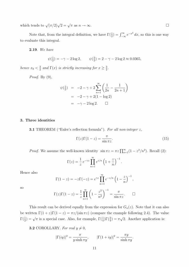
2.19. We have

ψ(12) = −γ − 2 log 2, ψ(3

2) = 2− γ − 2 log 2 ≈ 0.0365,

hence x0 <32

and Γ(x) is strictly increasing for x ≥ 32.

Proof. By (9),

ψ(12) = −2− γ + 2

∞∑n=1

(1

2n− 1

2n+ 1

)= −2− γ + 2(1− log 2)

= −γ − 2 log 2. �

3. Three identities

3.1 THEOREM (“Euler’s reflection formula”). For all non-integer z,

Γ(z)Γ(1− z) =π

sin πz. (15)

Proof. We assume the well-known identity sin πz = πz∏∞

n=1(1− z2/n2). Recall (2):

Γ(z) =1

ze−γz

∞∏n=1

ez/n(1 +

z

n

)−1

.

Hence also

Γ(1− z) = −zΓ(−z) = eγz

∞∏n=1

e−z/n(1− z

n

)−1

,

so

Γ(z)Γ(1− z) =1

z

∞∏n=1

(1− z2

n2

)−1

=π

sin πz. �

This result can be derived equally from the expression for Gn(z). Note that it can also

be written Γ(1 + z)Γ(1− z) = πz/(sin πz) (compare the example following 2.4). The value

Γ(12) =

√π is a special case. Also, for example, Γ(1

4)Γ(3

4) = π

√2. Another application is:

3.2 COROLLARY. For real y 6= 0,

|Γ(iy)|2 =π

y sinh πy, |Γ(1 + iy)|2 =

πy

sinh πy.

11

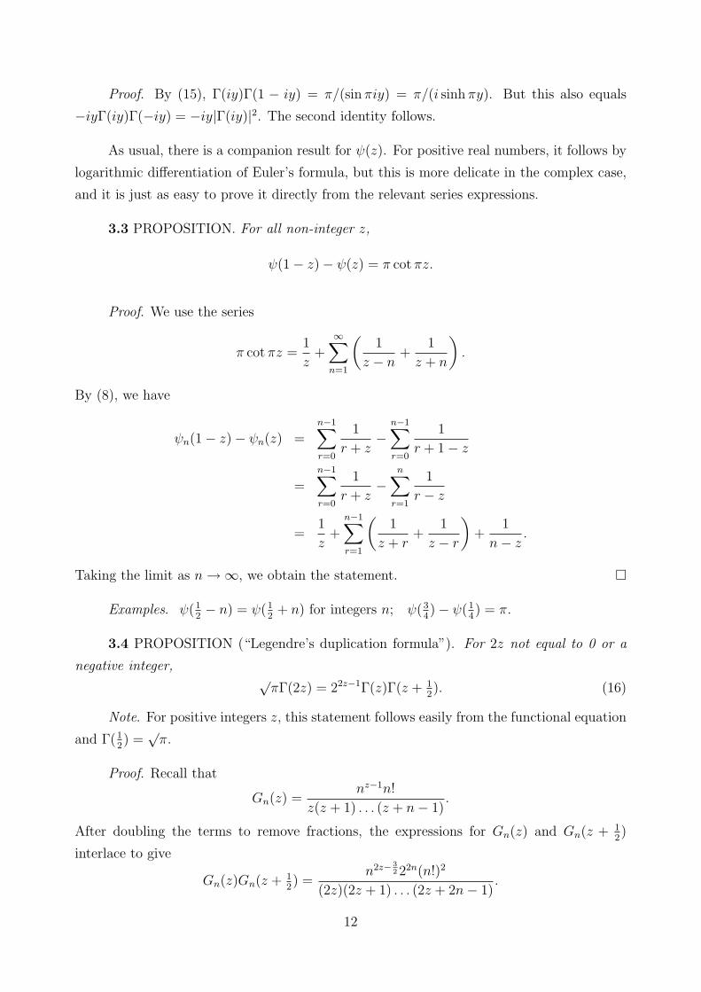
Proof. By (15), Γ(iy)Γ(1 − iy) = π/(sin πiy) = π/(i sinh πy). But this also equals

−iyΓ(iy)Γ(−iy) = −iy|Γ(iy)|2. The second identity follows.

As usual, there is a companion result for ψ(z). For positive real numbers, it follows by

logarithmic differentiation of Euler’s formula, but this is more delicate in the complex case,

and it is just as easy to prove it directly from the relevant series expressions.

3.3 PROPOSITION. For all non-integer z,

ψ(1− z)− ψ(z) = π cotπz.

Proof. We use the series

π cotπz =1

z+

∞∑n=1

(1

z − n+

1

z + n

).

By (8), we have

ψn(1− z)− ψn(z) =n−1∑r=0

1

r + z−

n−1∑r=0

1

r + 1− z

=n−1∑r=0

1

r + z−

n∑r=1

1

r − z

=1

z+

n−1∑r=1

(1

z + r+

1

z − r

)+

1

n− z.

Taking the limit as n→∞, we obtain the statement. �

Examples. ψ(12− n) = ψ(1

2+ n) for integers n; ψ(3

4)− ψ(1

4) = π.

3.4 PROPOSITION (“Legendre’s duplication formula”). For 2z not equal to 0 or a

negative integer,√πΓ(2z) = 22z−1Γ(z)Γ(z + 1

2). (16)

Note. For positive integers z, this statement follows easily from the functional equation

and Γ(12) =

√π.

Proof. Recall that

Gn(z) =nz−1n!

z(z + 1) . . . (z + n− 1).

After doubling the terms to remove fractions, the expressions for Gn(z) and Gn(z + 12)

interlace to give

Gn(z)Gn(z + 12) =

n2z− 32 22n(n!)2

(2z)(2z + 1) . . . (2z + 2n− 1).

12

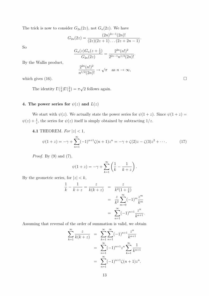
The trick is now to consider G2n(2z), not Gn(2z). We have

G2n(2z) =(2n)2z−1(2n)!

(2z)(2z + 1) . . . (2z + 2n− 1).

SoGn(z)Gn(z + 1

2)

G2n(2z)=

22n(n!)2

22z−1n1/2(2n)!.

By the Wallis product,22n(n!)2

n1/2(2n)!→√π as n→∞,

which gives (16). �

The identity Γ(14)Γ(3

4) = π

√2 follows again.

4. The power series for ψ(z) and L(z)

We start with ψ(z). We actually state the power series for ψ(1 + z). Since ψ(1 + z) =

ψ(z) + 1z, the series for ψ(z) itself is simply obtained by subtracting 1/z.

4.1 THEOREM. For |z| < 1,

ψ(1 + z) = −γ +∞∑

n=1

(−1)n+1ζ(n+ 1)zn = −γ + ζ(2)z − ζ(3)z2 + · · · . (17)

Proof. By (9) and (7),

ψ(1 + z) = −γ +∞∑

k=1

(1

k− 1

k + z

).

By the geometric series, for |z| < k,

1

k− 1

k + z=

z

k(k + z)=

z

k2(1 + zk)

=z

k2

∞∑m=0

(−1)m zm

km

=∞∑

n=1

(−1)n+1 zn

kn+1.

Assuming that reversal of the order of summation is valid, we obtain∞∑

k=1

z

k(k + z)=

∞∑k=1

∞∑n=1

(−1)n+1 zn

kn+1

=∞∑

n=1

(−1)n+1zn

∞∑k=1

1

kn+1

=∞∑

n=1

(−1)n+1ζ(n+ 1)zn.

13

The series∑∞

n=1 ζ(n + 1)|z|n converges for all z with |z| < 1, since ζ(n + 1) < 2 for all n.

Hence the double series is absolutely convergent, and the reversal is indeed valid. �

Alternatively, (17) follows from the values of ψ(n)(1) implied by repeated differentiation

as in 1.2.

Note. It is easily shown by integral estimation that ζ(m)− 1 ≤ 1/2m−1 for m ≥ 3. It

follows that the series∑∞

n=1(−1)n+1[ζ(n + 1) − 1]zn converges for |z| < 2. In the proof of

the theorem, if we first separate out the term k = 1, which contributes z/(1 + z), the term

ζ(n+ 1) is replaced by ζ(n+ 1)− 1 in the ensuing calculations, so we obtain

ψ(1 + z) = −γ +z

1 + z+

∞∑n=1

(−1)n+1[ζ(n+ 1)− 1]zn

for |z| < 2 (at z = −1, this holds in the sense of a limiting value, given the elementary fact

that∑∞

n=2[ζ(n)− 1] = 1).

Now consider L(z), as defined in section 1. Recall (Remark 4) that L(1 + z) = L(z) +

log z.

4.2 THEOREM. With L(z) defined as in Theorem 1.1, we have for |z| < 1

L(1 + z) = −γz +∞∑

n=2

(−1)n ζ(n)

nzn. (18)

Proof. By (5) and Remark 4, we have

L(1 + z) = −γz +∞∑

k=1

[zk− log

(1 +

z

k

)],

Now z − log(1 + z) =∑∞

n=2(−1)nzn/n, so

L(1 + z) = −γz +∞∑

k=1

∞∑n=2

(−1)n zn

nkn.

Reversing the order of summation as before, we obtain (18). �

Of course, differentiation of the series in (18) gives (17), so either of these series can

be used to prove the other.

Again, by separating out the term k = 1, we can deduce the following variant, valid

for |z| < 2 except for real z ≤ −1,

L(1 + z) = (1− γ)z − log(1 + z) +∞∑

n=2

(−1)n ζ(n)− 1

nzn.

14

This implies that (18) is also valid for z = 1. Since L(2) = 0, it equates to the identity

∞∑n=2

(−1)n ζ(n)

n= γ,

which can, of course, be proved more directly.

The power series for Γ(1 + z) is considerably less pleasant. The coefficients are best

expressed in terms of integrals. This series is discussed in separate notes ΓPS.

5. Alternative proof of convergence in the real case

We now present an attractive alternative proof of convergence of Gn(x) in the real

case, based on the principle that bounded, monotonic sequences converge. The method has

appeared in [Jam2]. It delivers some useful inequalities without further work. (However,

readers can omit or defer this section).

Define a companion sequence Hn(x) by

Hn(x) =(n+ 1)x−1n!

x(x+ 1) . . . (x+ n− 1).

Then Hn(1) = Hn(2) = 1 and

Hn(x) =

(1 +

1

n

)x−1

Gn(x).

Hence Gn(x) and Hn(x) have the same limit (if either converges), and Gn(x) < Hn(x) for

x > 1, while Gn(x) > Hn(x) for 0 < x < 1

We use the following well-known inequality:

5.1 LEMMA. For all t > 0, (1+t)p > 1+pt if p > 1, and (1+t)p < 1+pt if 0 < p < 1.

Proof. Let f(t) = (1 + t)p. By the mean-value theorem,

(1 + t)p − 1 = f(t)− f(0) = pt(1 + ξ)p−1

for some ξ ∈ (0, t). Clearly, (1 + ξ)p−1 > 1 if p > 1, and the reverse holds if 0 < p < 1: the

statement follows. �

5.2. (i) Gn(x) increases (strictly) with n for x > 1 and decreases for 0 < x < 1.

(ii) Hn(x) increases with n for x > 2 and for 0 < x < 1, and decreases for 1 < x < 2.

Proof. Let δn(x) = Gn+1(x)/Gn(x). Then

δn(x) =

(n+ 1

n

)xn

n+ x=

(1 +

1

n

)x (1 +

x

n

)−1

.

15

By the Lemma, δn(x) > 1 for x > 1 and δn(x) < 1 for 0 < x < 1.

Now let µn−1(x) = Hn(x)/Hn−1(x). Then

µn−1(x) =

(n+ 1

n

)x−1n

n+ x− 1=

(1 +

1

n

)x−1 (1 +

x− 1

n

)−1

.

By the Lemma, µn−1(x) > 1 for x > 2 and 0 < x < 1, while µn−1(x) < 1 for 1 < x < 2. �

We have already seen that Gn(x) is constant when x = 1, and Hn(x) is constant when

x = 1 and x = 2.

5.3 THEOREM. For all real x except 0 and negative integers, Gn(x) and Hn(x) tend

to a common limit (which we denote by Γ(x)) as n→∞. Furthermore, we have:

Hn(x) ≤ Γ(x) ≤ Gn(x) for 0 ≤ x ≤ 1, (19)

Gn(x) ≤ Γ(x) ≤ Hn(x) for 1 ≤ x ≤ 2, (20)

Gn(x) ≤ Hn(x) ≤ Γ(x) for x ≥ 2. (21)

Proof. First, let 1 ≤ x ≤ 2. Then Gn(x) is increasing, Hn(x) is decreasing and

Gn(x) ≤ Hn(x) for all n. Hence Gn(x) ≤ H1(x) for all n, so Gn(x) is bounded above,

hence convergent. As already noted, it follows that Hn(x) converges to the same limit.

Furthermore, it is clear that (20) holds. When 0 ≤ x ≤ 1, similar reasoning establishes

convergence and (19).

To deduce the statement for all other x, just note that convergence of Gn(x) to L

implies convergence of Gn(x + 1) to xL, and conversely. Repeated steps of length 1 (both

forwards and backwards) now establish convergence for other x. Also, (21) holds. �

Since xΓn(x) = Gn(x + 1), it follows that for all x > 0, Γn(x) increases with n and

Γn(x) ≤ Γ(x).

The inequality (19) can be rewritten as a pair of bounds for Γ(x) between integers.

Since x(x+ 1) . . . (x+ n− 1) = Γ(n+ x)/Γ(x), we have

Gn(x) = nx−1n!Γ(x)

Γ(n+ x), Hn(x) = (n+ 1)x−1n!

Γ(x)

Γ(n+ x).

Inserted into (19), this gives:

5.4 COROLLARY. For 0 ≤ x ≤ 1 and integers n ≥ 1,

(n+ 1)x−1n! ≤ Γ(n+ x) ≤ nx−1n!. (22)

16

For 1 ≤ x ≤ 2, these inequalities are reversed. �

We return to inequalities of this sort in section 6, where we will show that there is no

need for the restriction of n to integers.

Example. Given the value Γ(12) =

√π, the case x = 1

2in (19) equates to the following

specific form of the Wallis product:

(nπ)1/2 ≤ 2.4. . . . (2n)

1.3 . . . (2n− 1)≤ [(n+ 1)π]1/2.

All the identities in Theorem 1.1 can now be derived as before (with, of course, no

complication in the choice of log Γ(x)). Differentiability is proved as in Remark 3.

6. Inequalities for gamma function ratios; the Bohr-Mollerup theorem

This section follows the article [Jam1], with some additional results for ψ(x). The

objective is to find upper and lower bounds for the ratio Γ(x+ y)/Γ(x), which we denote by

R(x, y). A simple estimation follows easily from the fact (2.12) that log(x−1) ≤ ψ(x) ≤ log x:

6.1. For all x > 1 and y > 0,

(x− 1)y ≤ R(x, y) ≤ (x+ y)y. (23)

Hence R(x+ y) ∼ xy as x→∞ with y fixed.

Proof. By the mean-value theorem, log Γ(x + y) − log Γ(x) = yψ(ξ) for some ξ in

(x, x+ y). By 2.12, we have log(x− 1) ≤ ψ(ξ) ≤ log(x+ y). Inequality (23) follows, and it

clearly implies the last statement. �

With very little extra effort, we now derive more accurate estimations for R(x, y),

distinguishing the cases 0 ≤ y ≤ 1, 1 ≤ y ≤ 2 and y ≥ 2. Furthermore, we will use nothing

more than log-convexity and the functional equation. So we consider any function f(x),

defined for x > 0, that satisfies

(A) log f(x) is convex and f(x+ 1) = xf(x) for all x > 0.

By proceeding in this way, we will be able to use the results to establish that Γ(x) is in fact

the only function that satisfies (A) and f(1) = 1.

6.2. Suppose that f satisfies (A). Write R(x, y) = f(x+ y)/f(x). Then

R(x, y) ≤ xy for 0 ≤ y ≤ 1, (24)

17

R(x, y) ≥ xy for y ≥ 1 and for y < 0. (25)

Proof. For fixed x, let F (y) = log f(x+ y)− y log x for all y > −x. Then F is convex

and

F (1) = log f(x+ 1)− log x = log f(x) = F (0).

It follows that F (y) ≤ log f(x) for 0 ≤ y ≤ 1 and F (y) ≥ log f(x) for y ≥ 1 and for y ≤ 0.

This equates to (24) and (25). �

Note. A variant of this proof is as follows. Let L(x) = log f(x) and mL(x, y) =

[L(y) − L(x)]/(y − x). Clearly, mL(x, x + 1) = log x. If 0 < y < 1, then convexity of L

implies that mL(x, x + y) ≤ mL(x, x + 1), hence 1ylogR(x, y) ≤ log x, so R(x, y) ≤ xy. The

opposite holds when y > 1. �

Clearly, equality holds when y is 0 or 1, and if log f(x) is strictly convex, then strict

inequality holds for other y.

By suitable substitutions, we can deduce further bounds applying for various intervals

for y:

6.3. For f satisfying (A), we have

R(x, y) ≤ x(x+ 1)y−1 for 1 ≤ y ≤ 2, (26)

and the opposite holds for y ≤ 1 and y > 2. Also,

R(x, y) ≥ x(x+ y)y−1 for 0 ≤ y ≤ 1, (27)

and the opposite holds for y > 1.

Proof. For (26): if 1 ≤ y ≤ 2, then (24) gives

R(x+ 1, y − 1) =f(x+ y)

f(x+ 1)≤ (x+ 1)y−1,

so that f(x+ y) ≤ x(x+ 1)y−1f(x). By (25), the opposite holds for y ≤ 1 and y ≥ 2.

For (27): if 0 ≤ y ≤ 1, then (24) gives

R(x+ y, 1− y) =f(x+ 1)

f(x+ y)≤ (x+ y)1−y,

hence f(x+ y) ≥ x(x+ y)y−1f(x). By (25), the opposite holds for y ≥ 1. �

Note that both (26) and (27) are exact at the end points of the stated intervals for y.

18

We reassemble these inequalities for the three intervals for y, obtaining a comprehensive

system of bounds for R(x, y). In some cases, we choose the better of two options on offer:

6.4 THEOREM. For f satisfying (A), we have

x(x+ y)y−1 ≤ R(x, y) ≤ xy for 0 ≤ y ≤ 1, (28)

xy ≤ R(x, y) ≤ x(x+ 1)y−1 for 1 ≤ y ≤ 2, (29)

x(x+ 1)y−1 ≤ R(x, y) ≤ x(x+ y)y−1 for y ≥ 2. � (30)

If this seems complicated, reflect that we have arrived at it by a very simple process!

It is quite normal for inequalities involving powers to reverse at certain values of the index.

Note. To recapture the (weaker) lower bound (x− 1)y in (23), observe that by (25),

R(x− 1, y + 1) =f(x+ y)

f(x− 1)≥ (x− 1)y+1,

so f(x+ y) ≥ (x− 1)yf(x).

These inequalities have a curious history. In Artin’s book [Art], published in 1931, the

inequality (x− 1)y ≤ R(x, y) ≤ xy appears on p. 14 (actually stated for integer x), but only

as a step in the proof of the Bohr-Mollerup theorem. The method is essentially the one given

here. With no reference to Artin, and by a considerably longer method, Wendel proved (28)

in 1948 [Wen]. In 1959, with no reference to Artin or Wendel, and by a different method

again, Gautschi [Gau] obtained (28) with the weaker lower bound x(x + 1)y−1 (along with

another estimate in terms of ψ(x)). Later writers have generally referred to results of this

type as “Gautschi-type inequalities”, with scant respect to either Artin or Wendel.

These inequalities have numerous applications. First, we restate (28) specifically for

the gamma function in the case where x is a positive integer n, thereby obtaining bounds

for the gamma function between integers. Since Γ(n) = (n− 1)!, the statement becomes:

6.5. For positive integers n and 0 ≤ y ≤ 1,

(n+ y)y−1n! ≤ Γ(n+ y) ≤ ny−1n! for 0 ≤ y ≤ 1. � (31)

In 5.4, the same upper bound was found by a different method, together with the

slightly weaker lower bound (n+ 1)y−1n!.

Another application is to binomial coefficients. Let

Kn(y) = (−1)n

(−yn

)=

(n+ y − 1

n

)=y(y + 1) . . . (y + n− 1)

n!.

19

This is the coefficient of tn in the series for (1− t)−y. Clearly

Kn(y) =Γ(n+ y)

Γ(y)n!=R(n, y)

nΓ(y),

so by (28) and (29), we have:

6.6. We have

(n+ y)y−1

Γ(y)≤ Kn(y) ≤ ny−1

Γ(y)for 0 ≤ y ≤ 1,

ny−1

Γ(y)≤ Kn(y) ≤ (n+ 1)y−1

Γ(y)for 1 ≤ y ≤ 2.

A similar estimate for y > 2 can be derived from (30). These can be regarded as

bounds for Kn(y), with Γ(y) regarded as known.

Using Euler’s reflection formula (3.1), we can deduce bounds for Γ(y − n) that form a

natural companion to (31).

6.7. For 0 < y < 1 and integers n ≥ 1,

π

sin πy

ny

n!< (−1)nΓ(y − n) <

π

sin πy

(n+ 1)y

n!. (32)

Proof. By Euler’s formula,

Γ(y − n)Γ(n+ 1− y) =π

sin π(y − n)= (−1)n π

sin πy

and by (31), applied to 1− y, we have (n+ 1)−yn! < Γ(n+ 1− y) < n−yn!. �

Theorem 6.4, together with Euler’s limit, delivers very easily the following character-

isation of the real gamma function, known as the Bohr-Mollerup theorem. We use Gn(x),

together with the companion expression Hn(x) defined in section 5.

6.8 THEOREM. Suppose that f(x) is defined for x > 0 and: (i) log f(x) is convex,

(ii) f(x+ 1) = xf(x), (iii) f(1) = 1. Then f(x) = Γ(x).

Proof. It is clearly enough to prove the theorem for 1 < x < 2 (for consistency

with the current notation, we now write y for x). By (29), for integers n we then have

ny ≤ R(n, y) ≤ n(n+ 1)y−1. Clearly, f(n) = (n− 1)!, so

ny−1n! ≤ f(n+ y) ≤ (n+ 1)y−1n!.

Since f(n + y) = y(y + 1) . . . (y + n − 1)f(y), this equates to Gn(y) ≤ f(y) ≤ Hn(y), so

f(y) = limn→∞Gn(y) = Γ(y). �

20

We now describe, in less detail, analogous results for ψ(x). The corresponding quantity

to consider is ψ(x+ y)− ψ(x). As an easy consequence of 2.14, we have:

6.9. For x > 1 and y > 0,

y

x+ y≤ ψ(x+ y)− ψ(x) ≤ y

x− 1.

Proof. By the mean-value theorem, ψ(x+ y)− ψ(x) = yψ′(ξ) for some ξ ∈ (x, x+ y).

Since ψ′ is decreasing, 2.14 gives ψ′(ξ) ≤ ψ′(x) ≤ 1/(x−1), also ψ′(ξ) ≥ ψ′(x+y) ≥ 1/(x+y).

�

Now consider any function g, defined on the positive real line, that shares the following

properties of ψ:

(B) g is concave and g(x+ 1) = g(x) + 1x

for all x > 0.

6.10. Suppose that g satisfies (B), and write S(x, y) = g(x+ y)− g(x). Then

S(x, y) ≥ y

xfor 0 ≤ y ≤ 1, (33)

and the opposite holds for y ≥ 1 and for y ≤ 0. Further, for 0 < y < 1,

S(x, y) ≤ y(x+ 1)

x(x+ y). (34)

Hence S(x, y) → 0 as x→∞ with y fixed.

Proof. For fixed x, let G(y) = g(x + y) − y/x. Then G is concave and G(1) =

g(x+ 1)− 1x

= g(x) = G(0). Hence G(y) ≥ g(x) for 0 ≤ y ≤ 1 and G(y) ≤ g(x) for other y.

This equates to (33). For 0 < y < 1, we deduce further

S(x+ y, 1− y) = g(x+ 1)− g(x+ y) ≥ 1− y

x+ y

so that

g(x+ y)− g(x) ≤ 1

x− 1− y

x+ y=y(x+ 1)

x(x+ y).

�

This also implies the simpler upper bound y/(x−1). Suitable substitutions give further

inequalities for 1 < y < 2 and for y > 2: we leave this to the reader. Instead, we show that

the analogue of the Bohr-Mollerup theorem follows very easily:

6.11 PROPOSITION. If g satisfies (B), then g(x) = ψ(x) + c for some constant c.

21

Proof. Fix y > 0, and let g(n+ y)− g(n) = δn. By 6.10, δn → 0 as n→∞. By (B),

g(n) = g(1) +n−1∑r=1

1

r,

g(n+ y) = g(y) +1

y+

n−1∑r=1

1

r + y,

hence

g(y) = g(1)− 1

y+

n−1∑r=1

(1

r− 1

r + y

)+ δn.

By (9), the right-hand side tends to ψ(y) + g(1) + γ as n→∞. �

7. Equivalence of Euler’s limit and the integral definition

We now establish the equivalence of Euler’s limit with the integral definition Γ(z) =∫∞0tz−1e−t dt. It is elementary that this integral converges for all z with Re z > 0. We shall

present the proof in terms of Γn(z) rather than Gn(z).

7.1 LEMMA. For 0 ≤ t < n,(1− t2

n

)e−t ≤

(1− t

n

)n

≤ e−t.

Proof. From the series for ey and 1/(1− y), it is clear that 1 + y ≤ ey ≤ 1/(1− y) for

0 ≤ y < 1. Multiplying through by (1 − y)e−y, we obtain (1 − y2)e−y ≤ 1 − y ≤ e−y. Now

take the nth power:

(1− y2)ne−ny ≤ (1− y)n ≤ e−ny

for 0 ≤ y < 1. Now (1− a)n ≥ 1− na for 0 ≤ a < 1, so we can replace (1− y2)n by 1− ny2.

Substitute y = t/n to obtain the statement. �

Recall that the beta integral B(a, b) is defined by B(a, b) =∫ 1

0xa−1(1− x)b−1 dx for a,

b with Re a > 0 and Re b > 0. We assume the following well-known evaluation of B(a, n)

for positive integers n:

B(a, n) =(n− 1)!

a(a+ 1) . . . (a+ n− 1).

Hence Γn(z) = nzB(z, n+ 1).

7.2 THEOREM. For Re z > 0, we have

limn→∞

Γn(z) =

∫ ∞

0

tz−1e−t dt.

22

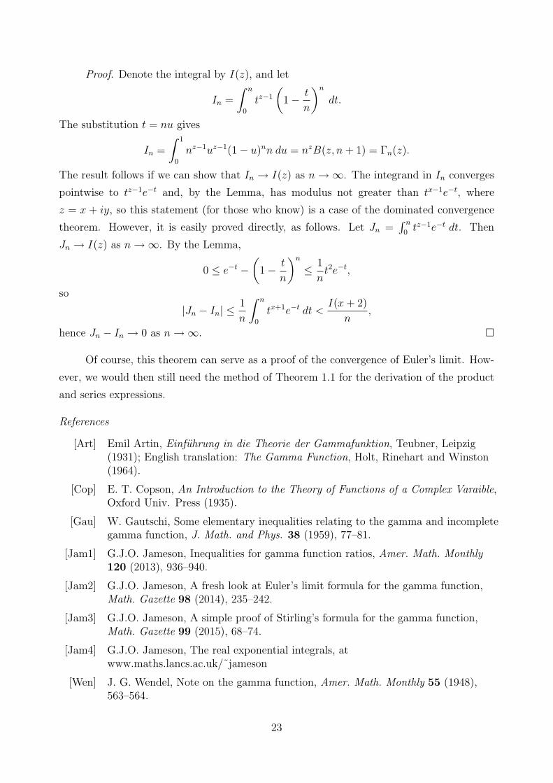
Proof. Denote the integral by I(z), and let

In =

∫ n

0

tz−1

(1− t

n

)n

dt.

The substitution t = nu gives

In =

∫ 1

0

nz−1uz−1(1− u)nn du = nzB(z, n+ 1) = Γn(z).

The result follows if we can show that In → I(z) as n→∞. The integrand in In converges

pointwise to tz−1e−t and, by the Lemma, has modulus not greater than tx−1e−t, where

z = x + iy, so this statement (for those who know) is a case of the dominated convergence

theorem. However, it is easily proved directly, as follows. Let Jn =∫ n

0tz−1e−t dt. Then

Jn → I(z) as n→∞. By the Lemma,

0 ≤ e−t −(

1− t

n

)n

≤ 1

nt2e−t,

so

|Jn − In| ≤1

n

∫ n

0

tx+1e−t dt <I(x+ 2)

n,

hence Jn − In → 0 as n→∞. �

Of course, this theorem can serve as a proof of the convergence of Euler’s limit. How-

ever, we would then still need the method of Theorem 1.1 for the derivation of the product

and series expressions.

References

[Art] Emil Artin, Einfuhrung in die Theorie der Gammafunktion, Teubner, Leipzig(1931); English translation: The Gamma Function, Holt, Rinehart and Winston(1964).

[Cop] E. T. Copson, An Introduction to the Theory of Functions of a Complex Varaible,Oxford Univ. Press (1935).

[Gau] W. Gautschi, Some elementary inequalities relating to the gamma and incompletegamma function, J. Math. and Phys. 38 (1959), 77–81.

[Jam1] G.J.O. Jameson, Inequalities for gamma function ratios, Amer. Math. Monthly120 (2013), 936–940.

[Jam2] G.J.O. Jameson, A fresh look at Euler’s limit formula for the gamma function,Math. Gazette 98 (2014), 235–242.

[Jam3] G.J.O. Jameson, A simple proof of Stirling’s formula for the gamma function,Math. Gazette 99 (2015), 68–74.

[Jam4] G.J.O. Jameson, The real exponential integrals, atwww.maths.lancs.ac.uk/˜jameson

[Wen] J. G. Wendel, Note on the gamma function, Amer. Math. Monthly 55 (1948),563–564.

23