1

Chapter 17: Amortized Analysis III

2

Dynamic Table

• Sometimes, we may not know in advance the #objects to be stored in a table

• We may allocate space for the table, say with malloc(), at the beginning

• When more objects are inserted, the space allocated before may not be enough

3

Dynamic Table

• The table must then be reallocated with a larger size, say with realloc(), and all objects from original table must be copied over into the new, larger table

• Similarly, if many objects are deleted, we may want to reallocate the table with a smaller size (to save space)

• Any good choice for the reallocation size?

4

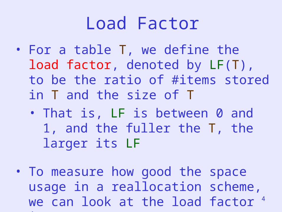
Load Factor• For a table T, we define the load

factor, denoted by LF(T), to be the ratio of #items stored in T and the size of T• That is, LF is between 0 and 1, and

the fuller the T, the larger its LF

• To measure how good the space usage in a reallocation scheme, we can look at the load factor it guarantees

5

Load Factor• Obviously, we have a reallocation

scheme that guarantees a load factor of 1:• Rebuild table for each indel

(insert/delete)

• However, n indels can cost (n2) time• In general, we want to trade some

space for time efficiency

• Can we ensure any n indels cost (n) time, and a not-too-bad load factor?

6

Handling Insertion• Suppose we have only insertion

operations• Our reallocation scheme is as follows:

If T is full before insertion of an item,we expand T by doubling its size

• It is clear that at any time, LF(T) is at least 0.5

• Question: How about the insertion cost?

7

Handling Insertion• Observe that the more items are

stored, the closer the next expansion will come

• Let num(T) = #items currently stored in T

• Let size(T) = size of T

• To reflect this observation, we define a potential function such that

T= 2 num(T) – size(T)

8

Handling Insertion• The function has some nice

properties: • Immediately before an expansion,

T= num(T) this provides enough cost to copy items into new

table

• Immediately after an expansion, T= 0

this resets everything, and simplify the analysis

• Its value is always non-negative (the table is always at least half full)

9

Amortized Cost of Insertion• Now, what will be amortized insertion

cost? • Notation

• ci = actual cost of ith operation

• i = amortized cost of ith operation

• numi = #items in T after ith operation

• sizei = size of T after ith operation

• i= Tafter ith operation

• There are two cases …

10

Case 1: No Expansion

• If ith insertion does not cause expansion:

i = ci + i- i-1

= 1 + (2numi – sizei) - (2numi-1 – sizei-1)

= 1 + 2numi - 2numi-1

= 3

11

Case 2: With Expansion

• If ith insertion causes an expansion: sizei =2sizei-1 and sizei-1 =numi-1 = numi – 1

i = ci + i- i-1

= numi + (2numi – sizei) - (2numi-1 – sizei-1)

= numi + (2numi– 2(numi – 1)) - (2(numi

– 1) – (numi – 1))

= numi + 2- (numi – 1)

= 3

Conclusion: amortized cost for insertion = O(1)

12

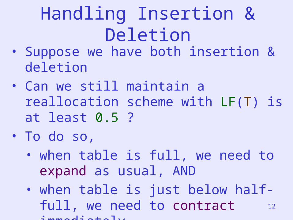
Handling Insertion & Deletion

• Suppose we have both insertion & deletion

• Can we still maintain a reallocation scheme with LF(T) is at least 0.5 ?

• To do so, • when table is full, we need to expand

as usual, AND• when table is just below half-full, we

need to contract immediately

13

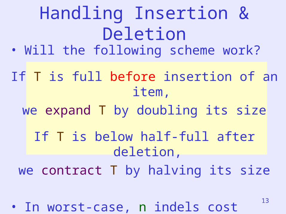
Handling Insertion & Deletion

• Will the following scheme work?

If T is full before insertion of an item,we expand T by doubling its size

If T is below half-full after deletion, we contract T by halving its size

• In worst-case, n indels cost (n2) time

14

Slight Modification• The previous scheme fails because we

are too greedy … (contracting too early)

• Let us modify our scheme slightly:If T is full before insertion of an item,

we expand T by doubling its size

If T is below (1/4)-full after deletion, we contract T by halving its size

• At any time, LF(T) is at least 0.25

15

Handling Insertion & Deletion

• Now, using this scheme,• If table is more than (1/2)-full, we

should start worrying about the next expansion watch for insertion

• If table is less than (1/2)-full, we should start worrying about the next contraction watch for deletion

• This gives us some intuition of how to define the potential function

16

New Potential Function• Our new potential function is a bit

strange (it has two parts):

• If table is at least half full: T= 2 num(T) – size(T)

• If table is less than half full:

T= size(T)/2 – num(T)

• Can you compute the amortized cost for each operation?

17

Nice Properties• The function has some nice

properties: • Immediately before a resize,

T= num(T) this provides enough cost to copy items into new

table

• At half-full or immediately after resize,

T= 0 this resets everything, and simplify the analysis

• Its value is always non-negative

18

Amortized Insertion Cost• If ith operation = insertion • If it causes an expansion:

i = same as before = 3

• If it does not cause expansion:

• if T at least half full, (LFi-1 < ½ , LFi ≥ ½)

i = same as before = 3

• if T less than half full,i = ci + (sizei/2 – numi) - (sizei-1/2 – numi-1) = 1 + (-1) = 0

19

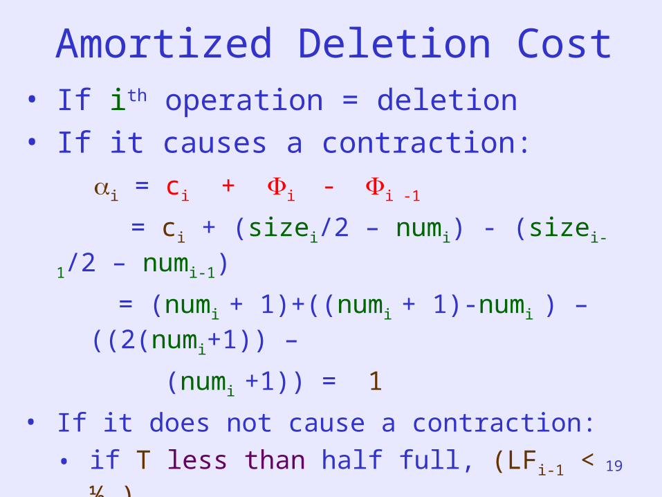
Amortized Deletion Cost• If ith operation = deletion • If it causes a contraction: i = ci + i- i -1

= ci + (sizei/2 – numi) - (sizei-1/2 – numi-1)

= (numi + 1)+((numi + 1)-numi ) – ((2(numi+1)) –

(numi +1)) = 1

• If it does not cause a contraction:

• if T less than half full, (LFi-1 < ½ )

i = ci + (sizei/2 – numi) - (sizei-1/2 – numi-1)

= 1 + 1 = 2

20

Amortized Deletion Cost (cont)

• If it does not cause a contraction:

• if T at least half full, (LFi-1 ≥ ½)

i = ci + i- i -1

= ci + (2numi – sizei) - (2numi-1 – sizei-

1)

= 1 - 2 = -1This operation will not

cause any problem

21

Conclusion

• The amortized insertion or deletion cost in our new scheme = O(1)

• Meaning: Any n operations in total cost O(n) time

• Remark: There can be other reallocation schemes with O(1) load factor and O(1) amortized cost (Try to

think about it !)

22

Homework

• Problem: 17-2 (Due: Dec. 7)• Practice ay home: 17.1-3, 17.2-1,

17.3-3, 17.3-6, 17.4-1 • Second Mid-Term Exam. Dec. 9• Ch 19 Fibonacci heaps (Self-study)

23

Quiz 3

• Show that the second smallest of n elements can be found with n + lg n - 2 comparisons in the worst case.

• Give an O(n)-time Dynamic Programming algorithm to compute the n-th Fibonacci number.