1

CA202Spreadsheet Application

Performing Calculation on Data

Lecture # 3

ByDammam Community college

2

Objectives

• Naming group of data

• Creating formulas to create values

• Finding and correcting errors in calculation

3

Naming Group of Data

• Select the range including top heading, then – Insert Name Create

• Top row is selected as name

• You can use this name in formula e.g. =SUM(Price)

4

Naming Group of Data

• Another way to name the range is:– Insert Name Define

• Top row will be used as range name

• You can use this name in formula e.g. =CountA(Product_Name)

5

Naming Group of Data

• Final way to name the range is:– Select the range– Click in the Name box next

to formula bar, then type the name of range

– You can use this name in formula e.g. =SUM(Price)

6

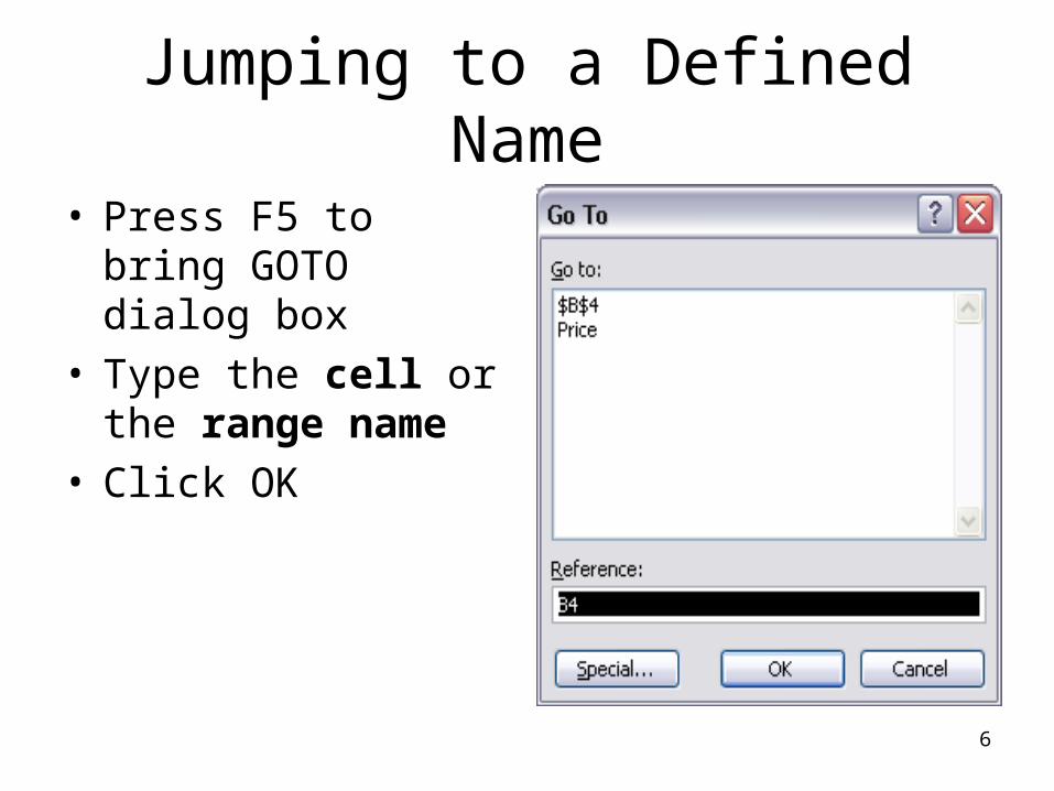
Jumping to a Defined Name

• Press F5 to bring GOTO dialog box

• Type the cell or the range name

• Click OK

7

Naming Conventions

• Maximum range name can be up to 255 characters

• Name must not be identical to cell address

• First character must be letter or underscore

• It’s not case sensitive

• Try to use Initial Cap e.g. AcctPayable

8

Labels as Range Name

• You can set labels as range name

• Choose Accept labels in formulas

Select

9

Referring to Cell in your formula

• =A1 into cell B2, B2 will show the value of A1, whenever Excel re-calculate the value

• Referring to range of cells e.g. B4:U8

Operator Type of cell Reference

Example

: Range A3:C19

, Comma, for union A3:C19, D34:D39

A single space Intersection X10:X20 W5:X11

Space

10

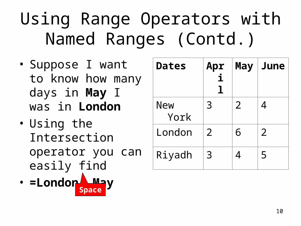
Using Range Operators with Named Ranges (Contd.)

• Suppose I want to know how many days in May I was in London

• Using the Intersection operator you can easily find

• =London May

Dates April May June

New York 3 2 4

London 2 6 2

Riyadh 3 4 5

Space

11

Using Range Operators with named Ranges

• The union operator is probably less often useful

• Suppose if I need to know total number of days I was out in May and the days I had in London during the entire 2nd Quarter

• The formula will look like as follow:• =SUM (London, May) – London May• 16 will be displayed

12

Automatic and Manual Calculation (Contd.)

• Any time you change or edit your spreadsheet Excel recalculate your formulas to keep them updated

• Tools Options Calculation tab set the calculation automatic or manual

• With manual calculation on, Press F9 to calculate all open worksheets or Shift + F9 to calculate the active worksheet only

13

Recalculate before Save

• By setting manual calculation, you can move around complex worksheet quickly

• Check the box labeled “Recalculate before save” guarantee, your data will be updated when you save

• All open workbooks use the same calculation mode

• Calculation mode is not saved with workbook or template

14

How does Excel calculate formulas?

• Excel normally uses the underlying stored value for calculation, No matter how many decimal places are shown or hidden

• To force Excel to calculate using the value displayed in your worksheet rather than underlying stored value

• You can set Tools → Options → Calculation Tab → precision as Displayed

• You can set this option for each workbook differently

15

View Formula instead of results

• To see contents of all the formulas, press Toggle Ctrl + ` (back quote), every column in your worksheet get widens and display formulas

• Or • Tools → Options →

View tab and turning on the formulas Select

16

Creating Formula

• Must begin with an equal ( = ) sign

17

Using the formula palette

• Palette does not appear when you press = sign to start a formula or F2 to edit one

• Type the valid function name, and before typing brackets, press Ctrl + A

18

Using the formula palette

• After typing the valid function name, press Ctrl + Shift + A to insert the argument list and parenthesis but does not display the formula palette

19

Using the formula palette

• Choose Insert → Function

20

Operators for your formula

• Formula consist of at least 2 numbers or cell reference

• Formula is nothing more than equal sign followed by a value

• % (percent) 10% results in 0.1• ^ (exponent) 4^3 (64)• & concatenates two value “Foot” & “ball”

(Football) into a single string

21

Relative versus Absolute reference

• By default cell values are relative e.g. C5, B2 etc

• Relative cell formula changes, when copies on other location of Excel

• To create an absolute cell reference add a $ character before row and column e.g. $A$1

• You can add the dollar sign to only one coordinate e.g. $A1 or A$1

22

Cell reference outside the worksheet

• To refer a cell or range in another worksheet of workbook– Precede the cell address with the sheet name

followed by an ! Exclamation marks– e.g. =SUM (‘Spring Sales’!C2:C5)

• To refer a cell or range of another workbook List the workbook in square brackets, followed by the sheet name, the exclamation point, and the cell reference– e.g. =SUM (‘[Toy Sale] Spring Sales’!C2:C5)

23

Finding formula precedent with the Range finder

• When you edit formula on worksheet, Excel gives you visual cues to formulas and their precedents

• This is the job of range finder• Each formula reference in the formula is

highlighted with different color, Ranges matches the similar color too

• To change cell or range use drag handle• Either Drag the border itself or select a new

range

24

Information FunctionFunction Explanation

COUNTBLANK The number of blank cell in a range

ISBLANK True if specified cell is blank

ISEVEN True if specified cell contain even number

ISTEXT True if specified cell contain text

TYPE Return number representing type of data cell contain, 1 for number, 2 for text

25

Logical FunctionFunction Explanation

AND TRUE if all the arguments are true, otherwise FALSE

IF If true, 1st value otherwise 2nd value

NOT TRUE if the input argument is FALSE

OR TRUE if any of the argument are TRUE, FLASE if both are not TRUE

26

Date and Time Function

Function Explanation

DATE The Date, Year, month and Day

DAY The Integer corresponding to the Day of month

NOW Current Date and Time according to your PC

WEEKDAY The day of Week for a specified date value

WORKDAY The date value for the next workday after a specified start day

27

Lookup Reference Function

Function Explanation

COLUMN The number of Columns in a range

ROWS The number of Rows in a range

MATCH The relative position of an item you are searching for in a range (not the value)

28

Math and Trigonometry Function

Function Explanation

ABS The absolute value of the input

ROUND The input number rounded off to a specified number of digits

SIGN 1 if the input number is positive, 0 if the number is zero, -1 if the number is negative

SQRT The square root of the input value

TRUNC The integer portion of the input value, truncating any decimal position

29

Text Function

Function Explanation

CLEAN The input text without non printing characters

DOLLAR Convert numeric value into currency format

LEFT A specified number of characters starting at the LEFT side of the input string

MID A specified number of characters starting at the MID side of the input string

RIGHT A specified number of characters starting at the RIGHT side of the input string

30

Text FunctionFunction Explanation

LEN The number of Characters in the input text string

LOWER The text converted to LOWER case

UPPER The text converted to UPPER case

TEXT Convert a number into corresponding text formatted according to specified pattern

TRIM The text with all extra spaces removed

31

Statistical FunctionFunction Explanation

AVERAGE The arithmetic mean of the arguments

COUNT The number of cells containing numeric values within the input range

MAX The largest value in a series

MIN The lowest value in a series

32

Database and List Management Function

Function Explanation

DCOUNT The number of records matching your criteria

DMAX The maximum value of those records matching your criteria

DSUM The sum of the values in a field for all records matching your criteria

33

DSUM example

34

Using IF function

• IF (logical test, true_value, false_value)

• IF (TodaySales>1000,”Celebrate”,”Ordinary Day”)

• IF (JackPot>3000000,IF(Weekday(Today())=7,”Wed Special”,”Big JackPot”),”Meager Winning)

35

Finding and Correcting Errors in Calculations

• Error Code Description• ##### The column isn’t wide enough to display the

value.• #VALUE! The formula has the wrong type of argument

(such as text where a TRUE or FALSE value is required).

• #NAME? The formula contains text that Excel doesn’t recognize (such as an unknown named range).

• #REF! The formula refers to a cell that doesn’t exist (which can happen whenever cells are deleted).

• #DIV/0! The formula attempts to divide by zero.

36

Using the Auditing Toolbar

• Choose Tools Formula Auditing Toolbar

• Cell precedent are the cell that provide data to the formula in the active cell

• Cell dependent are those that depends on the value in the active cell

• 5 + 4 = 9, Here 9 is dependent and 5 and 4 are the precedent

37

Formula Auditing Toolbar

• On Auditing toolbars Click Trace precedents, a blue tracer arrows indicate cells that are precedents

• Cells from other worksheets are indicated by arrows with a small worksheet icon

• To find the cells in formula simply double click anywhere along the arrows

38

Tracing Won’t Work on the Followings

• You can’t trace the following referenced items with the auditing tools– Text boxes– Embedded charts– Pivot Charts– Pictures– Pivot Table– Dependent cells residing in a closed workbook

• Tracers are graphical objects, you won’t see them if objects are hidden on the worksheet

• Tools Options View Tab Show All

39

Removing Tracer Arrows

• Select the formula cell and click the Remove Precedent Arrow button to remove arrow

• To remove all tracer arrows, click the Remove All Arrows button

40

The double-click trick

• Tools Options Edit Tab Edit Directly in cell

• Once you have turned off in cell editing, you can double click any formula to immediately select are precedent cells

• If you double click a formula with a remote reference (i.e. a reference to another workbook), the workbook opens and the precedent cell is selected

41

For Keyboard Users

Keyboard shortcuts

Explanation

Ctrl + [ Select direct precedents of the current cell

Ctrl + Shift + [ Select direct/indirect precedents of the current cell

Ctrl + ] Select direct dependents of the current cell

Ctrl + Shift + ] Select direct/indirect dependents of the current cell

42

Cell Error Messages

Error Meanings

#DIV/0! The formula is dividing by zero

#N/A A value is not available to the function or formula

#NAME? Text in the formula is not recognized

#NULL! The formula refers to an intersection of two areas that do not intersect

#NUM! A problem occurs with a number in the formula or function

#REF! A cell reference is not valid

#VALUE! A wrong type of argument or operand is used

##### A formatted number is too wide to display in column

43

Tracing Error

• Select the cell that has error• Click the Trace Error button. Red arrow point the

formula that cause error value• Blue arrows point to cell containing values that

create error• Double-Click the arrow to select and display the

cell at the other end of an arrow• Excel stop tracing at the branch point when you

use Trace Error• To continue tracing, Click TRACE Error Again

44

Parenthesis matching in formula

• Excel now display parenthesis in color as they are entered

• Outermost pain is black• Inner as displayed in a series of up to 7 different

colors• When typing a closing parenthesis, the pair is

momentarily highlighted• IF the parenthesis are already entered, move the

cursor across one to highlight the pair

45

Common Error Message, #NAME?

• If you have a formula full of functions and defined Names to find which one is causing problem– Always enter formula in Lower Case– All defined name an Initial Cap

• When you enter formula, excel goes through an error checking routine, it does 2 things– Convert all recognized function name to upper case– It convert all recognized defined name to the case in which they

were defined– If you‘ve defined name in Initial Cap, and entered in formula in

Lower Case, #NAME? error will keep that function and defined name in lower case

46

Using the formula bar as calculator

• Complex formula can pass Excels error checkpoint but still deliver wrong or suspect result

• To find the problem is to calculate one partition at a time

• In formula bar select one piece of the function– Press F9– Only that portion is calculated, and the result appear

in the formula bar– You can do this to other part of the formula– After calculating the desired portion, press Esc to

restore the original formula

47

Chapter 3 Key Points

1. Creating named ranges lets you refer to entire blocks of cells with a single name1. Be sure you use absolute referencing ($A$1) if you want

the formula to remain the same when it’s copied2. You can use the Insert Function dialog box to help you on

your way3. You can monitor how the value in a cell changes by

adding a watch to the watch window4. To see which formulas refer to the values in the selected

cell, use Trace Dependents;5. if you want to see which cells provide values for the

formula in the active cell, use Trace Precedents6. You can step through the calculations of a formula in the

Evaluate Formula dialog box