1

Basics2

2

Outline

Review of data structuresData frames• Review of data frame structure• Importing/Exporting• Data frame example• Browsing • Selecting/Subsetting • Manipulating• Table and unique functions• Merging• Summarizing with apply, by, aggregate

Basic Programming• if/else• for/while loops• functions• Summarizing with functions

Graphics• Scatterplots• Histograms• Barplots• Pie Charts

3

## Initialize R Environment

# Set working directory..setwd("C:/Rworkshop")getwd()

# Create a new folder named 'Outfolder' in working directoryif(!file.exists("Outfolder")){ dir.create("Outfolder") }

# Set optionsoptions(scipen=6) # bias against scientific notation

# Load librarieslibrary(RODBC) # ODBC database interface

Initialize R Environment

4

Get Sample Data

## Get Sample data

# Load sample data files from website (SampleData_PartI.zip)http://www.fs.fed.us/rm/ogden/research/Rworkshop/SampleData.shtml

# Extract zip file to working directoryunzip("SampleData_PartI.zip")

# List files in folderlist.files("PlotData")

5

# vector group of single objects or elements (all elements must be the same mode)

# factors vector of values that are limited to a fixed set of values (categories)

# list group of objects called components(can be different modes and lengths)

# array group of vectors with more than 1 dimension (all elements must be the same mode)format: array(data=NA, dim=c(dim1, dim2, ..)

# matrix 2-dimensional array (group of vectors with rows and columns)

(all elements must be the same mode).format: matrix(data=NA, nrow=1, ncol=1, byrow=FALSE)

# data frame 2-dimensional list (group of vectors of the same length)

(can be different modes) format: data.frame(row, col)

R Data Structures

Images from: https://www.stat.auckland.ac.nz/~paul/ItDT/HTML/node64.html

6

Data Frames Review

## Data frames are the primary data structure in R.

## Data frames are used for storing data tables, such as forest inventory data tables.

## A data frame is similar structure to a matrix, except a data frame may contain categorical data, such as species names.

## Each column of a data frame is treated as a vector component of a list and therefore, can be different modes. The difference is that each vector component must have same length.

7

# data frame 2-dimensional list (group of vectors of the same length; can be different modes)# data.frame(row, column)

## Start with a matrixmat <- matrix(data=c(seq(1,5), rep(2,5)), nrow=5, ncol=2)

df <- data.frame(mat) # Convert matrix to data frameis.data.frame(df) # Check if object is a data framedim(df) # Get dimensions of data framestr(df) # Get structure of data framematv <- c(mat) # Create a vector from matrixis.vector(matv)dflst <- c(df) # Create a list from data frameis.list(dflst)

## Accessing elements of a data frame## Data frames can be accessed exactly like matrices, but they can also be accessed by

column names.

df[1,2] # Identify value in row 1, column 2df[3,] # Identify values in row 3 (vector)df[,2] # Identify values in column 2 (vector)df[2:4,1] # Identify values in rows 2 thru 4 and column 1 (vector)

df[3,"X2"] # Identify value in row 3, column 2df[,"X2"] # Identify values in column 2('X2')df[2:4,"X1"] # Identify values in column 2 thru 4 and column 1('X1')

Data Frames Review

8

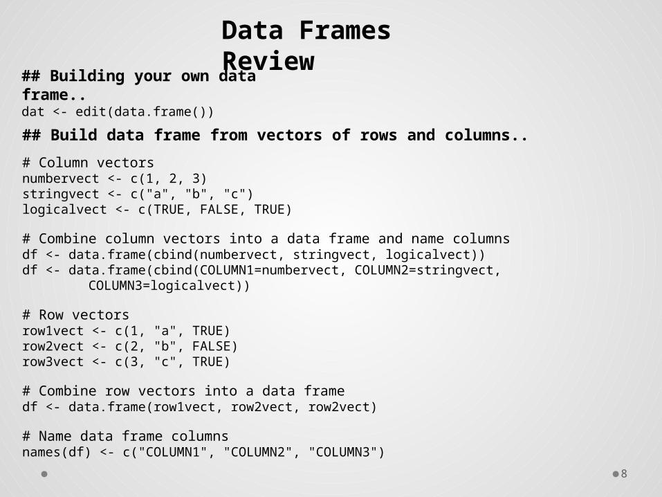
## Build data frame from vectors of rows and columns..

# Column vectorsnumbervect <- c(1, 2, 3)stringvect <- c("a", "b", "c")logicalvect <- c(TRUE, FALSE, TRUE)

# Combine column vectors into a data frame and name columnsdf <- data.frame(cbind(numbervect, stringvect, logicalvect))df <- data.frame(cbind(COLUMN1=numbervect, COLUMN2=stringvect,

COLUMN3=logicalvect))

# Row vectorsrow1vect <- c(1, "a", TRUE)row2vect <- c(2, "b", FALSE)row3vect <- c(3, "c", TRUE)

# Combine row vectors into a data framedf <- data.frame(row1vect, row2vect, row2vect)

# Name data frame columnsnames(df) <- c("COLUMN1", "COLUMN2", "COLUMN3")

## Building your own data frame..dat <- edit(data.frame())

Data Frames Review

9

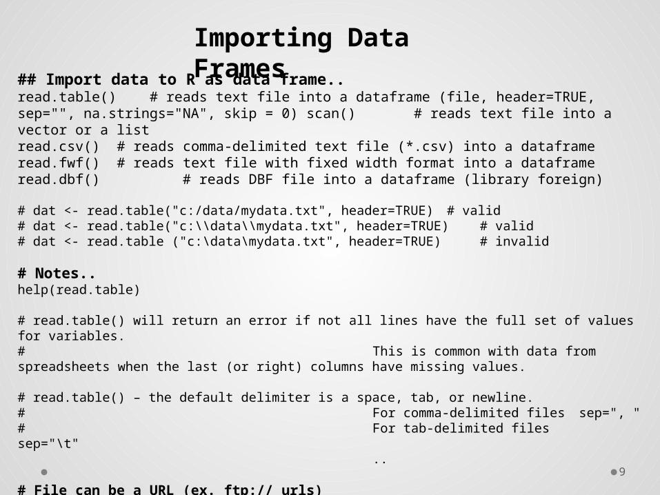
## Import data to R as data frame..read.table() # reads text file into a dataframe (file, header=TRUE, sep="", na.strings="NA", skip = 0) scan() # reads text file into a vector or a listread.csv() # reads comma-delimited text file (*.csv) into a dataframeread.fwf() # reads text file with fixed width format into a dataframeread.dbf() # reads DBF file into a dataframe (library foreign)

# dat <- read.table("c:/data/mydata.txt", header=TRUE) # valid# dat <- read.table("c:\\data\\mydata.txt", header=TRUE) # valid# dat <- read.table ("c:\data\mydata.txt", header=TRUE) # invalid

# Notes..help(read.table)

# read.table() will return an error if not all lines have the full set of values for variables. # This is common with data from spreadsheets when the last (or right) columns have missing values.

# read.table() – the default delimiter is a space, tab, or newline. # For comma-delimited files sep=", " # For tab-delimited filessep="\t"

..

# File can be a URL (ex. ftp:// urls)# dat <- read.csv("ftp://ftp2.fs.fed.us/incoming/rmrs/testdat.csv", header=TRUE)

Importing Data Frames

10

## Excel files..# It is recommended to export the data from Excel to a tab-delimited or comma-

separated file before importing to R.

# Convert long numbers represented with scientific notation to a number or a text before exporting (using Format Cells..).

# Check imported dataframe in R for entire rows or columns of NA values… from extraneous empty cells.

## Missing Values..# By default, only blanks are read as missing values. If you have some other

indication for a missing value, you need to let R know what that missing value character is by specifying na.strings (ex. na.strings="" or na.strings="." ).

Importing Data Frames

11

## Package: RODBC# channel <- odbcConnect(dsn) # Data Source Name (dsn)# channel <- odbcConnectAccess("filenm.mdb") # ACCESS database # channel <- odbcConnectAccess2007("filenm.accdb") # ACCESS database (2007, 2010)# channel <- odbcConnectExcel("filenm.xls") # Excel workbook (*.xlsx??)# channel <- odbcConnectExcel("filenm.xlsx") # Excel workbook (2007, 2010)# channel <- odbcConnect(dsn="idbfia.mci") # Oracle database (need Oracle driver)# channel <- odbcConnect("mydb1", case="postgresql")

# PostgreSQL database (need PostgreSQL driver)# Note: If channel = -1 , something is wrong

# Get data..# Set channel to path of Excel spreadsheetchannel <- odbcConnectExcel("PlotData/testdat.xls")

# Get list of tables (sheets) in spreadsheetsqlTables(channel)

# Fetch data from Excel spreadsheet (using sqlFetch or sqlQuery)testdat <- sqlFetch(channel, "testdat") # Specify sheet namedat <- sqlQuery(channel, "select PLT_CN, TREE from [testdat$]")

odbcClose(channel) # Close connection (frees resources)odbcDataSources() # Displays available data source names (dsn)http://cran.r-project.org/web/packages/RODBC/vignettes/RODBC.pdf

Importing Data Frames

12

## Exporting data from R..

# write.table() # writes a dataframe to a text file (append = FALSE, sep=" ")# write.csv() # writes a dataframe to a comma-delimited text file (*.csv) # write.dbf() # writes a dataframe to a DBF file (library foreign)

write.table(testdat, "Outfolder/testdat2.txt") write.table(testdat, "Outfolder/testdat2.txt",

row.names=FALSE, sep=",")write.csv(testdat, "Outfolder/testdat2.csv", row.names=FALSE)

# Notes..help(write.table)

# The default settings include row names and column names and has a space delimiter.

# write.table() – the default delimiter is a space, tab, or newline. # For comma-delimited files:

sep=", " # For tab-delimited files:

sep="\t"

Exporting Data Frames

13

PLT_CN unique plot number (numero parcela unico)TREE unique tree # (numero arbol unico)STATUSCD live/dead (codigo de estado (vivir/muertos))SPCD species code (estado arbol)DIA diameter - inches (dap)HT height - feet (altura)BA basal area sqft (area basal)

## Read in sample data frame..setwd("C:/Rworkshop") # use path to your Rworkshopdat <- read.csv("PlotData/testdat.csv", header=TRUE, stringsAsFactors=FALSE)

dat # Display dat. Check if data frame has extra rows of NA values.

Data Frame Example

14

Data Frames - Browsing

## Browsing data frames

dat # Print dataframe to screenView(dat) # Display dataframe in spreadsheet formatdat <- edit(dat) # Edit dataframe in spreadsheet format

head(dat) # Display first rows of dataframe (default = 6 rows)head(dat, n=10) # Display first 10 rows of dataframetail(dat) # Display last rows of dataframe (default = 6 rows)names(dat) # Display column names of datrow.names(dat) # Display row names of datsummary(dat) # Display summary statistics for columns of datstr(dat) # Display internal structure of dat

## Dimensions of data frames

dim(dat)nrow(dat)ncol(dat)

15

## Selecting and subsetting columns and rows in data frames - df[rows, cols)

# To define or select data frame columns: df$colnm or df[,colnm]# To define or select data frame rows: df[rowid, ]

dat[, c("TREE", "DIA")] # Select TREE and DIA columns for all rowsdat[3:5,] # Select all columns for rows 3 thru 5dat[c(4,6), c(2:4)] # Select rows 4 and 6 and columns 2 thru 4 dat[dat$SPCD == 746,] # Select all columns where SPCD = 746dat[dat$DIA < 10,] # Subset rowssubset(dat, DIA < 10) # Subset rowsdfsub <- subset(dat, DIA<10) # Assign new data frame object to subset of datdfsub # Display dfsub

# Select the TREE and DIA columns for dead trees onlydat[dat$STATUSCD == 2, c("TREE", "DIA")]

# Select columns where SPCD=746 and STATUSCD=2 dfsub[dfsub$SPCD == 746 & dfsub$STATUSCD == 2, ]

Data Frames – Selecting/Subsetting

16

## Manipulating data in data frames..

# To remove column(s) from data framedfsub$HT <- NULL # Removes one columndfsub[,!(names(dfsub) %in% c("TREE", "DIA"))] # Removes one or more columns

# To change name of a column in a data framenames(dat)[names(dat)== "SPCD"] <- "SPECIES"

# To order a dataframe dat <- dat[order(dat$SPECIES, dat$DIA),] # Order by 2 columnsdat <- dat[order(dat$DIA, decreasing=TRUE),] # Descending orderdat <- dat[order(dat$PLT_CN),] # Order by 1 column

Data Frames - Manipulating

17

## Manipulating data in data frames cont..

# To add a column of concatenated columnsdat$NEW <- paste(dat$TREE, ":", dat$SPECIES) # With default spacesdat$NEW <- paste(dat$TREE, ":", dat$SPECIES, sep="") # With no spaces

# .. with leading 0 valuesdat$NEW <- paste(dat$TREE, ":", formatC(dat$SPECIES,width=3,flag=0),sep="")

# To add a column of percent of total basal area for each tree in dat (rounded).dat$BApertot <- round(dat$BA / sum(dat$BA) * 100, 2)

Data Frames - Manipulating

18

## Exploring data frames with the unique and table functions..

# Display the unique values of species in dataset and sortunique(dat$SPECIES)sort(unique(dat$SPECIES))

# Display the number of trees by specieshelp(table)tab <- table(dat$SPECIES)class(tab)

# Display the number of trees by species and plottable(dat$PLT_CN, dat$SPECIES)table(dat[,c("PLT_CN", "SPECIES")])data.frame(table(dat$PLT_CN, dat$SPECIES))

# Create an object with the number of trees by status, species, and plot # .. and add column namestabdf <- data.frame(table(dat$PLT_CN, dat$SPECIES, dat$STATUSCD))names(tabdf) <- c("PLT_CN", "SPECIES", "STATUSCD", "FREQ")

# Get a count of dead tree species by plottable(dat[dat$STATUSCD == 2, "SPECIES"], dat[dat$STATUSCD==2, "PLT_CN"])table(dat[dat$STATUSCD ==2, "PLT_CN"], dat[dat$STATUSCD == 2, "SPECIES"])

Data Frames - Exploring

19

## More ways to explore data frames..

# Get the maximum height (HT) for Douglas-fir (SPECIES=202)max(dat[dat$SPECIES == 202, "HT"])

# Get the average height (HT) for both Douglas-fir (SPECIES=202) and lodgepole pine (SPECIES=106)mean(dat[dat$SPECIES %in% c(202, 108), "HT"])

# Get the average diameter (DIA) for dead (STATUSCD=2) aspen trees (SPECIES=746)mean(dat[(dat$SPECIES == 746 & dat$STATUSCD == 2), "DIA"])

# Get the average diameter (DIA) for live (STATUSCD=1) aspen trees (SPECIES=746)mean(dat[(dat$SPECIES == 746 & dat$STATUSCD == 1), "DIA"])

Data Frames - Exploring

20

# Example: merge variable code descriptions for species to data frame

1. Get data frame of code descriptions2. Merge to table

Data Frames - Merging

21

# Example: merge variable code descriptions for species to data frame

## First, get data frame of code descriptions# Build species look-up table (or import from file)

# Gets unique values of species, sorted:SPECIES <- sort(unique(dat$SPECIES))SPECIESNM <- c("subalpine fir", "Engelmann spruce", "lodgepole pine", "Douglas-fir", "aspen")sptab <- data.frame(cbind(SPECIES, SPECIESNM))

## Then, merge to tablehelp(merge)dat <- merge(dat, sptab, by="SPECIES")dat

dat[order(dat$PLT_CN, dat$TREE), ]

Data Frames - Merging

22

Exercise 7

## 7.1. Load testdat.csv again, assigning it to object ex1df.

## 7.2. Display the dimensions, the column names, and the structure of ex1df.

## 7.3. Display the first 6 rows of ex1df.

## 7.4. Display this table ordered by heights with the largest trees first and display the maximum height.

## 7.5. Change name of column STATUS to 'ESTADO', DIA to 'DAP', and column HT to 'ALTURA'.

## 7.6. Merge the sptab table we made on slide 18 to the ex1df table, using the SPCD column, and assign to ex1df2. Hint: use by.x and by.y for merging to columns with different names.

## 7.7. Display only rows with subalpine fir and DAP greater than 10.0.

## 7.8. Display the number of trees by ESTADO and SPECIESNM.

## 7.9. Display the total basal area (BA) for lodgepole pine.

23

Exercise 7 cont.

## 7.10. Create a new object named 'aspen' with just the rows in ex1df2 that are aspen.

## 7.11. The 2 columns, SPCD and SPECIESNM, are not important in the aspen table. Remove them and overwrite object 'aspen'.

## 7.12. Display the mean ALTURA of live aspen trees.

## 7.13. Create a look up table for ESTADO and merge this table to ex1df2. Assign the merged table to ex1df3. Then order ex1df3 by PLT_CN.

## Hint:## 1. Get vector of unique values of ESTADO## 2. Define new vector called ESTADONM where 1 = Live and 2 = Dead ## 3. Create dataframe of vectors with names ESTADO and ESTADONM## 4. Merge new dataframe to ex1df2## 5. Order table by PLT_CN and TREE

## 7.14. Display the number of trees again, this time by ESTADONM and SPECIESNM.

24

Summarizing Data Frameswith apply, by, aggregate

25

apply – applies a function to rows or columns of an array, matrix, or data frame (returns a vector or array).

sapply – applies a function to each element of a list or vector (returns a vector or array).

lapply – similar to sapply, applies a function to each element of a list or vector (returns a list).

tapply – applies a function to a vector, separated into groups defined by a second vector or list of vectors (returns an array).

by – similar to tapply, applies a function to vector or matrix, separated in to groups by a second vector or list vectors (returns an array or list).

aggregate – applies a function to one or more vectors, separated into groups defined by a second vector or list of vectors (returns a data frame).

Function Input Outputapply array/matrix/data frame vector/arraysapply vector/list vector/arraylapply vector/list listtapply vector array/matrixby data frame array/listaggregate data frame data frame

Summarizing Data Frames

26

# apply – applies a function to the rows or columns of an array, matrix, or data frame

# (1-rows; 2-columns).

# Apply a mean across 3 columns of dat meandat <- apply(dat[,c("DIA", "HT", "BA")], 2, mean)meandatis.vector(meandat) # Returns a vector

# sapply/lapply – applies a function to a each element of a list or vector.

# Check if columns of dat are numericis.list(dat)sapply(dat, is.numeric) # Returns a vectorlapply(dat, is.numeric) # Returns a list

# Display the number of characters for each column name of dat.sapply(names(dat), nchar)

apply, lapply, sapply

27

tapply - applies a function to a vector, separated into groups defined by a second

vector or list of vectors (returns an array/matrix).

## Get max DIA for each SPECIESNM.maxdia <- tapply(dat$DIA, dat$SPECIESNM, max)maxdiaclass(maxdia)is.vector(maxdia)

# Get summed basal area by species and plot.spba.tapply <- tapply(dat$BA, dat[,c("PLT_CN", "SPECIESNM")], sum)spba.tapplydim(spba.tapply)class(spba.tapply)is.array(spba.tapply)

# Change NA values to 0 (0 basal area) and round all values to 2 decimal places.spba.tapply[is.na(spba.tapply)] <- 0spba.tapply <- round(spba.tapply, 2)spba.tapply

## Accessing output of tapplyspba.tapply[1,]spba.tapply["4836418010690",]spba.tapply["4836418010690", "lodgepole pine"]

tapply

28

## Now, let's add one more variable.. and summarize by STATUSCD as well.

stspba.tapply <- tapply(dat$BA, dat[,c("PLT_CN", "SPECIESNM", "STATUSCD")], sum)stspba.tapply[is.na(stspba.tapply)] <- 0stspba.tapplyclass(stspba.tapply)

## Accessing output of tapplydim(stspba.tapply) # An array with 3 dimensions[1] 2 5 2 #(PLT_CN, SPECIESNM, STATUSCD)

# Display all elements of dimensions 2 and 3, for the first element of dimension 1.stspba.tapply[1,,]stspba.tapply["4836418010690",,] # ..or the name of the element

# Display all elements of dimensions 1 and 3, for the third element of dimension 2.stspba.tapply[,3,]stspba.tapply[,"Engelmann spruce",] # ..or the name of the element

# Display all elements of dimensions 1 and 2, for the second element of dimension 3.stspba.tapply[,,2]stspba.tapply[,,"2"] # ..or the name of the element

# Display one element of array.stspba.tapply[2,4,2]stspba.tapply["40374256010690","lodgepole pine","2"]

tapply cont..

29

by – applies a function to vector or matrix, separated in to groups by a second vector or list of vectors (returns a by class(array/list(if simplify=FALSE)).

## Get max DIA for each SPECIESNM

## The default by statement returns an object of class 'by'maxdia <- by(dat$DIA, dat$SPECIESNM, mean)maxdiaclass(maxdia)is.list(maxdia)

## Accessing output from by (default)maxdia[1] # Display element 1maxdia[[1]] # Display value of element 1maxdia[["aspen"]] # Display value of element named 'aspen'

## Adding simplify=FALSE, returns on object of class list or arraymaxdia2 <- by(dat$DIA, dat$SPECIESNM, mean, simplify=FALSE)maxdia2class(maxdia2)is.list(maxdia2)

## Accessing is the same as above, except you can also use '$', because it is a list.maxdia2[1] # Display element 1maxdia2[[1]] # Display value of element 1maxdia2[["aspen"]] # Display value of element named 'aspen'maxdia2$aspen

by

30

# Get summed basal area by species and plotspba.by <- by(dat$BA, dat[,c("PLT_CN", "SPECIESNM")], sum, simplify=FALSE)spba.by[is.na(spba.by)] <- 0spba.by class(spba.by)is.list(spba.by)dim(spba.by)

## Accessing output from by statement (same as tapply, except can use list option)dim(stspba.by) # An array(list) with 2 dimensions[1] 2 5 #(PLT_CN, SPECIESNM)

# Display all elements of dimensions 2, for the first element of dimension 1.spba.by[1,]spba.by["4836418010690",] # ..or the name of the element

# Display all elements of dimension 1, for the forth element of dimension 2.spba.by[,4]spba.by[,"lodgepole pine"] # ..or the name of the element

# Display one element and element value from array/list.spba.by[2,4] # Elementspba.by["40374256010690","lodgepole pine"] # Elementspba.by[,"lodgepole pine"]$"40374256010690" # Element valuespba.by["40374256010690",]$"lodgepole pine" # Element value

by cont..

31

by – applies a function to vector or matrix. tapply – applies a function to a vector only.

# Use by to apply a function to more than one variable. How correlated are DIA, BA, and HT for each species?

by(dat[,c("DIA", "BA", "HT")], dat$SPECIESNM, cor)

by cont..

32

aggregate – applies a function to one or more vectors, separated into groups defined by a second vector or list of vectors (returns a data frame).

# Get sum of basal area by plotsumbaspp <- aggregate(dat$BA, list(dat$SPECIESNM), sum)names(sumbaspp) <- c("SPECIESNM", "SUMBA")

# Get sum of basal area by plot and STATUSCDspba.ag <- aggregate(dat$BA, list(dat$PLT_CN, dat$SPECIESNM), sum)class(spba.ag)

# Add names to data framenames(spba.ag) <- c("PLT_CN", "SPECIESNM", "SUMBA")

# Get average diameter and average height by SPECIESNMavgdiahtspp <- aggregate(dat[,c("DIA", "HT")], list(dat$SPECIESNM), mean)names(avgdiahtspp) <- c("SPECIESNM", "AVGDIA", "AVGHT")

# Merge summed basal area by species with average dia/height by speciesdatsum <- merge(sumbaspp, avgdiahtspp, by="SPECIESNM")

aggregate

33

## Differences in output

# Example: Get the number of trees by plot

# Using tapplytreecnt <- tapply(dat$PLT_CN, dat$PLT_CN, length)treecntclass(treecnt)

# Using bytreecnt.by <- by(dat$PLT_CN, dat$PLT_CN, length)treecnt.by class(treecnt.by)is.array(treecnt.by)

# Using aggregatetreecnt.ag <- aggregate(dat$PLT_CN, list(dat$PLT_CN), length)names(treecnt.ag) <- c("PLT_CN", "NUM_TREES")class(treecnt.ag)treecnt.ag

# Using table functiontreecnt.tab <- table(dat$PLT_CN)treecnt.tabclass(treecnt.tab)is.array(treecnt.tab)

Comparison of Summary Functions

34

## 8.1 Use sapply to change the names of dat to all upper case letters.

## 8.2 Use apply to get the range of values for DIA and HT in dat. Set the results to an object named 'ranges'. Is this object an array? What is the class of 'ranges'?

## 8.3 Use tapply to get the minimum 'HT' by SPECIESNM and STATUSNM and set to an object named minht. Change any NA values to 0.

## 8.4 Use aggregate to get a sum of BA by SPECIESNM. Set this to an object named 'ba.sum'. Add names to ba.sum, SPECIESNM, SUMBA. What is the class of 'ba.sum'?

Exercise 8

35

Basics Programming in R

36

# Example: Print to screen if the value x is less than, equal to, or greater than 10.x <- 5if(x < 10){

print("less than 10")}else if(x == 10){

print("equals 10")}else{

print("greater than 10")}

# Assign x to 10 and run the if statement again.x <- 10

if/else statements## Format

# if(logical statement1){# then statement1# }else if(logical statement2){# then statement2# }else{# then statement3# }

37

# Example: Print to screen if the value x is less than 10 or greater than or equal to 10.x <- 5answer <- ifelse(x < 10, "less than 10", "greater than or equal to 10")answer

x <- 10ifelse(x < 10, "less than 10", "greater than or equal to 10")

# Example: Append a new column named STATUSNM to dat with 2 values, "live", where STATUSCD = 1, and "dead", where STATUSCD = 2.

dat$STATUSNM <- ifelse(dat$STATUSCD == 1, "live", "dead")

ifelse statement

## Format# ifelse(logical statement1, yes, no)

38

# Example: for loopfor(i in 1:10){

print(i)}

# Example: while loopi <- 1while(i < 10){

print(i)i <- i + 1

}

# Example: for loopweekdays <- c("Mon", "Tues", "Wednes", "Thurs", "Fri", "Satur", "Sun")for(day in weekdays){

print(paste(day, "day", sep=""))}

## Format # for(i in 1:n){# execute statement# }

for/while loops

39

## IFELSE statements and FOR loops

# Example: Create a loop using the previous example for if/else statements.

for(x in 1:20){if(x < 10){

print("less than 10")}else if(x == 10){

print("equals 10")}else{

print("greater than 10")}

}

# Example: Create a loop that compiles a vector with column names of dat that are less than 5 characters wide.

datnames <- vector()for(name in names(dat)){

name.length <- nchar(name)if(name.length < 5){

datnames <- c(datnames, name)}

}datnames

if/else and for loops

40

# Example: Create a function using the previous example, with x as a user-defined parameter.

getx <- function(x){if(x < 10){

print("less than 10")}else if(x == 10){

print("equals 10")}else{

print("greater than 10")}

}getx(5)getx(10)

# Example: Function to perform 2 calculations and return the result.getx2 <- function(x, y){

x2 <- x * yx2 <- x2 + 5return(x2) }

x2 <- getx2(5, 100)getx2(2, 20)

# Format # f <- function(<arguments>) {# Do something interesting# }

Functions

41

# Example: Function to print the mean diameter of a specified species.meanDIA <- function(SPECIES){

# Gets mean DIA for SPECIES in datdia.mean <- mean(dat[dat$SPECIES == SPECIES, "DIA"])

# Gets name for SPECIES in datspnm <- unique(dat[dat$SPECIES == SPECIES, "SPECIESNM"])

paste("Mean diameter for", spnm, "is:", round(dia.mean)) }meanDIA(108)meanDIA(746)

# Example: Function to print the mean of a specified variable for a specified species.meanval <- function(SPECIES, var){

# Gets mean var for SPECIES in datvar.mean <- mean(dat[dat$SPECIES == SPECIES, var])

# Gets name for SPECIES in datspnm <- unique(dat[dat$SPECIES == SPECIES, "SPECIESNM"])

paste("Mean", var, "for", spnm, "is:", round(var.mean))}meanval(746, "HT")meanval(108, "DIA")

Functions cont.

42

# Example: Function to print the specified function of a specified variable for a specified species. The default function is mean.

funval <- function(SPECIES, var, funnm=mean){# Summarizes var by funnm for SPECIES in datvar.mean <- funnm(dat[dat$SPECIES == SPECIES, var])

# Gets name for SPECIES in datspnm <- unique(dat[dat$SPECIES == SPECIES, "SPECIESNM"])

# Gets the string name for the functionfunnm <- deparse(substitute(funnm))

paste(funnm, var, "for", spnm, "is:", round(var.mean))}funval(746, "HT", mean)funval(746, "HT")funval(108, "BA", sum)

Functions cont.

43

# Example: Function to return a table of pfun applied to pvar by xvar and yvar.

datPivot <- function(dat, pvar, xvar, yvar, pfun=sum){

ptab <- tapply(dat[,pvar], dat[,c(xvar, yvar)], pfun)ptab[is.na(ptab)] <- 0

return(ptab)}

datPivot(dat, "BA", "PLT_CN", "SPECIESNM")datPivot(dat, "HT", "PLT_CN", "SPECIESNM")datPivot(dat, "HT", "PLT_CN", "SPECIESNM",mean)

# Help on functionshttps://ems-team.usda.gov/sites/fs-fia-iw-tt/R%20Help%20docs/Rfunctions.pdf

Functions cont.

44

# Create a function to use with an apply statement to calculate a percent of the total basal area for multiple variables by species.

# First, create a table summarizing multiple variables by species.sptab <- aggregate(dat[,c("DIA", "BA")], list(dat$SPECIESNM), sum)names(sptab) <- c("SPECIESNM", "SUMDIA", "SUMBA")sptab

# Then, create a function to calculate percentages by species.perfun <- function(x){ round(x / sum(x) * 100, 2) }

# Apply this function on all columns of sptabapply(sptab[,-1], 2, perfun)

Summarizing with Functions

45

# Use the perfun function to calculate a percent of total basal area per plot.

# First, create a table summarizing BA by species and plotsppltba <- aggregate(dat$BA, list(dat$SPECIESNM, dat$PLT_CN), sum)sppltbanames(sppltba) <- c("SPECIESNM", "PLT_CN", "SUMBA")sppltba

# Then use a by statement to calculate percent basal area per speciessppltba.by <- by(sppltba$SUMBA, sppltba$PLT_CN, perfun)sppltba.by

# Append the percent calculation to sppltba.sppltba$BApercplot <- unlist(sppltba.by)sppltba

# Check the column totals by plotby(sppltba$BApercplot, sppltba$PLT_CN, sum)

Summarizing with Functions

46

## 9.1 Use the sapply function to determine if any columns of dat are factors.

## 9.2 Create a loop to check if any of the columns of dat is a factor. Print to screen the name of the columns that are factors.

## 9.3 Append a column named HTCLASS to dat with 2 categories: "SHORT "or "TALL", use the mean of HT as the break point.So: for trees with HT less than the mean HT, set HTCLASS = "SHORT", and

for trees with HT greater than or equal to the mean HT, set HTCLASS = "TALL". Check if this works using a table on HT and HTCLASS.

## 9.4 Create a function named 'getrows', that will print out all the records (or trees) of dat for a specified SPECIES. Include one parameter named 'sp'. How many records have lodgepole trees (108)?

## 9.5. Using the function you created in 9.4, how many records have aspen trees? What is the average HT for these records (trees)?

## 9.6 Create a function to use with sapply to add a "_1" to all the column names of dat.

Exercise 9

47

A Touch on Graphics in R

48

Scatterplots# Plot a scatterplot of basal area by heightplot(dat$BA, dat$HT)

help(plot)help(par) # Help on graphical parameterspar() # Display current settings of par

## Add labelsplot(dat$BA, dat$HT, main="Basal Area by Height", xlab="Basal Area", ylab="Height")

## Change symbol (see below)plot(dat$BA, dat$HT, main="Basal Area by Height", xlab="Basal Area", ylab="Height", pch=19)

## Change color and size of pointsplot(dat$BA, dat$HT, main="Basal Area by Height", xlab="Basal Area", ylab="Height", pch=19, col="red", cex=0.5)

pch

colors() # List of color choicescex <- 0.5# Make the symbol half the size

49

Scatterplots# Add multiple plots to graphics device (display window).par(mfrow=c(1,3)) # 1*3 = 3 plots (1 row, 3 columns)

## Add plotsplot(dat$BA, dat$HT, main="Basal Area by Height", xlab="Basal Area",

ylab="Height")plot(dat$BA, dat$HT, main="Basal Area by Height", xlab="Basal Area",

ylab="Height", pch=19)plot(dat$BA, dat$HT, main="Basal Area by Height", xlab="Basal Area",

ylab="Height", pch=19, col="red", cex=0.5)

# Change width of space surrounding plots in graphics device (display window).

# mar Number of lines of margin to be specified on all 4 sides of plot. # Default is c(5, 4, 4, 2) + 0.1 (bottom, left, top, right).

par(mfrow=c(1,3), mar=c(5, 6, 4, 2))

## Add plotsplot(dat$BA, dat$HT, main="Basal Area by Height", xlab="Basal Area",

ylab="Height")plot(dat$BA, dat$HT, main="Basal Area by Height", xlab="Basal Area",

ylab="Height", pch=19)plot(dat$BA, dat$HT, main="Basal Area by Height", xlab="Basal Area",

ylab="Height", pch=19, col="red", cex=0.5)

50

Scatterplots cont.

par(mfrow=c(1,1))

plot(dat$BA, dat$HT, main="Basal Area by Height", xlab="Basal Area", ylab="Height", pch=19, col="red", cex=0.5)

# Add fit lines to scatterplot to look at trendsabline(lm(dat$HT ~ dat$BA)) # Regression line (y~x)lines(lowess(dat$BA, dat$HT), col="green") # lowess line (x,y)

# Scatterplot matrixpairs(dat[,c("BA", "HT", "DIA")])

help(pairs)

## Other graphics packages# car# scatterplot3d

51

Histogramshelp(hist)

# Frequency Histogram

# Displays the frequency of observations (DIA).par(mfrow=c(1,3))hist(dat$DIA)hist(dat$DIA, breaks=2)hist(dat$DIA, breaks=2, ylim=c(0,10), main="Histogram of DIA", xlab="DIA")

# Probability Histogram

# Displays the probabilities (density) associated with all observations (DIA).par(mfrow=c(1,2))hist(dat$DIA, main="Frequency Histogram")hist(dat$DIA, prob=TRUE, main="Probability Histogram")

# Density curve of observationspar(mfrow=c(1,1))plot(density(dat$DIA))

# Overlay density curve on probability histogrampar(mfrow=c(1,1))hist(dat$DIA, prob=TRUE)lines(density(dat$DIA))

52

Barplotshelp(barplot)

## Create a barplot of total basal area by speciespar(mfrow=c(1,1))

# Get sum of basal area by species (using aggregate). spbasum.ag <- aggregate(dat$BA, list(dat$SPECIESNM), sum)names(spbasum.ag) <- c("SPECIESNM", "SUMBA")

## Create barplotbarplot(spbasum.ag$SUMBA)barplot(spbasum.ag$SUMBA, names.arg= spbasum$SPECIESNM, main="Sum of Basal Area - aggregate")

# Get sum of basal area by species (using tapply) and create barplot.spbasum.t <- tapply(dat$BA, dat$SPECIESNM, sum)barplot(spbasum.t, main="Sum of Basal Area - tapply")

## Add colorsbarplot(spbasum.t, col=c("yellow", "dark green", "blue", "orange", "red"), main="Sum of Basal Area - tapply") barplot(spbasum.t, col=rainbow(5), main="Sum of Basal Area - tapply")help(rainbow)

## Make x and y axes labels smallerbarplot(spbasum.t, col=c("yellow", "dark green", "blue", "orange", "red"),

cex.axis=0.75, cex.names=0.75, space=0.1, ylim=c(0,3.0))

53

Pie Charts## Create a pie chart of the proportion of basal area by species.help(pie)

# Use the table we created previouslysptab <- aggregate(dat[,c("DIA", "BA")], list(dat$SPECIESNM), sum)names(sptab) <- c("SPECIESNM", "SUMDIA", "SUMBA")sptab

# Calculate the proportion of SUMBA by speciespropba <- round(sptab$SUMBA / sum(sptab$SUMBA), 2)

## Create pie chartpar(mfrow=c(1,1))pie(propba, labels=sptab$SPECIESNM)

## Now lets create a pie chart for each plot we measured.# Again, use the table we created previously, with BApercplot

sppltba <- aggregate(dat$BA, list(dat$SPECIESNM, dat$PLT_CN), sum)names(sppltba) <- c("SPECIESNM", "PLT_CN", "SUMBA")sppltba$BApercplot <- unlist(by(sppltba$SUMBA, sppltba$PLT_CN, perfun))

par(mfrow=c(1,2))for(cn in unique(sppltba$PLT_CN)){

plt <- sppltba[sppltba$PLT_CN == cn,]pie(plt$BApercplot, labels=plt$SPECIESNM, cex=0.75, main=cn)

}

54

Exercise 10

## 10.1 Create a scatterplot of BA vs. DIA with proper labels. Are these variables correlated?

## 10.2 Add a regression line to the scatterplot in 10.1 and color it red.

## 10.3 Create a histogram of HT with 5 breaks and labels. What is the range of heights with the highest frequency?

## 10.4 Create a barplot of maximum heights by species with labels. Which species has the maximum height?

55

R Help Links

# List of available packages in Rhttp://cran.r-project.org/web/packages/available_packages_by_name.html

# Link to help on RODBC packagehttp://cran.r-project.org/web/packages/RODBC/vignettes/RODBC.pdf

# Data manipulationhttps://science.nature.nps.gov/im/datamgmt/statistics/r/fundamentals/manipulation.cfm

# apply/sapply/aggregate/..http://lamages.blogspot.com/2012/01/say-it-in-r-with-by-apply-and-friends.html

# R Programminghttp://en.wikibooks.org/wiki/R_Programming/

# Help on functionshttps://ems-team.usda.gov/sites/fs-fia-iw-tt/R%20Help%20docs/Rfunctions.pdf

# R Reference Cardhttp://scicomp.evergreen.edu/docs/workshops/RReferenceCard.pdf