1

An Efficient Algorithm for Optimally Solving

a Shortest Vector Problem in

Compute-and-Forward Design

Jinming Wen, Baojian Zhou, Student Member, IEEE, Wai Ho Mow,

Senior Member, IEEE, and Xiao-Wen Chang

Abstract

We consider the problem of finding the optimal coefficient vector that maximizes the computation

rate at a relay in the compute-and-forward scheme. Based on the idea of sphere decoding, we propose a

highly efficient algorithm that finds the optimal coefficient vector. First, we derive a novel algorithm to

transform the original quadratic form optimization problem into a shortest vector problem (SVP) using

the Cholesky factorization. Instead of computing the Cholesky factor explicitly, the proposed algorithm

realizes the Cholesky factorization with only O(n) flops by taking advantage of the structure of the

Gram matrix in the quadratic form. Then, we propose some conditions that can be checked with O(n)

flops, under which a unit vector is the optimal coefficient vector. Finally, by taking into account some

useful properties of the optimal coefficient vector, we modify the Schnorr-Euchner search algorithm to

solve the SVP. We show that the estimated average complexity of our new algorithm is O(n1.5P

0.5)

flops for i.i.d. Gaussian channel entries with SNR P based on the Gaussian heuristic. Simulations show

that our algorithm is not only much more efficient than the existing ones that give the optimal solution,

but also faster than some best known suboptimal methods. Besides, we show that our algorithm can be

readily adapted to output a list of L best candidate vectors for use in the compute-and-forward design.

The estimated average complexity of the resultant list-output algorithm is O(

n1.5

P0.5 logL+ nL

)

flops

for i.i.d. Gaussian channel entries.

Jinming Wen is with the Laboratoire de l’Informatique du Parallelisme, (CNRS, ENS de Lyon, Inria, UCBL), Universite de

Lyon, Lyon 69007, France (e-mail: jwen@math.mcgill.ca).

Baojian Zhou and Wai Ho Mow are with The Department of Electronic and Computer Engineering, Hong Kong University

of Science and Technology, Clear Water Bay, Kowloon, Hong Kong (e-mail: bzhouab, eewhmow@ust.hk).

X.-W. Chang is with The School of Computer Science, McGill University, Montreal, QC H3A 2A7, Canada (e-mail:

chang@cs.mcgill.ca).

2

Index Terms

Wireless relay network, slow-fading, compute-and-forward, computation rate, Cholesky factoriza-

tion, shortest vector problem, sphere decoding.

I. INTRODUCTION

In relay networks, compute-and-forward (CF) [1] is a promising relaying strategy that can offer

higher rates than traditional ones (e.g., amplify-and-forward, decode-and-forward), especially in

the moderate SNR regime. The crucial idea of CF is the application of linear/lattice codes [2]

and physical layer network coding (PLNC) [3]. The received signal at a relay is the linear

combination of a set of transmitted signals, where the linear combination coefficients form the

channel vector from the involved sources to that relay. Through multiplying the channel vector

by an amplifying factor, the obtained new channel vector can be close to a coefficient vector with

all integer-valued entries. This means that after applying an appropriate amplifying factor to the

received signal at a relay, it will be approximately an integer linear combination of the transmitted

signals. Since the same linear code is used at the sources, an integer linear combination of valid

codewords is still a valid codeword, which means the aforementioned integer linear combination

of the transmitted signals is possible to be successfully decoded as a linear combination of the

messages corresponding to the transmitted signals. Under certain conditions, with a sufficient

number of such decoded linear combinations, the transmitted messages can be recovered.

Obviously, the amplifying factors and the integer-valued coefficient vectors need to be carefully

designed. When Nazer and Gastpar proposed the CF scheme in [1], they defined the computation

rate, which refers to the maximum transmission rate at the involved sources of a relay such

that the combined signals at the relay can be reliably decoded. Transmission rate, which is the

minimum computation rate over all relays, determines the system performance. The transmission

rate becomes 0 if the coefficient matrix formed with rows being the coefficient vectors at the

relays is not of full rank [1]. It has been pointed out that setting the amplifying factor at a

relay as the minimum-mean-square-error (MMSE) coefficient can maximize the computation

rate at that relay. The difficulty lies in the design of the coefficient vectors. To optimize the

system performance, the coefficient vectors have to be designed jointly. However, this requires

each relay (or the destination instead) to know the channel state information (CSI) at the other

relays, which could incur too much communication overhead in practice for large networks. Also,

3

the joint optimization problem could be far too complex to solve. One alternative is to firstly

develop a search algorithm to find good coefficient vectors at each relay with the criterion being

maximizing the computation rate at that relay, and then apply a certain strategy to coordinate

relays in selection of the coefficient vectors. This is reasonable when only the local CSI is

available at each relay, or when the network is large. Unfortunately, the problem is difficult

even for finding the coefficient vector that maximizes the computation rate at one relay, as it

turns out to be a shortest vector problem (SVP) in a lattice. In this paper, we shall first focus

on developing the search algorithm for finding the optimal coefficient vector at a relay (defined

as the one that maximizes the computation rate at that relay). After that, we will show how to

adapt our algorithm such that it can be used for solving the CF design problem.

The SVP of finding the optimal coefficient vector at a relay has attracted a lot of research

interests, and various methods have been proposed to solve the problem. The Fincke-Pohst

method [4] was modified in [5] to solve a different but related problem, leading to the optimal

coefficient vector and some other suboptimal vectors. A branch-and-bound algorithm, which uses

some properties of the optimal vector, was proposed in [6]. But it appears that this algorithm is not

very efficient in this application. There are some more efficient methods that give suboptimal

solutions. Three suboptimal methods were proposed in [7]: a method based on the complex

LLL [8], a simple quantized search method, which has been improved in [9], and an iterative

MMSE-based quantization method. Although the average complexity of the LLL algorithm [10]

is polynomial if the entries of the basis vectors independently follow the normal distribution

N (0, 1) (see, e.g., [11], [12]), the complexity of the first method could be too high since it has

been proved in [11] that in the MIMO context, the worst-case complexity of the LLL algorithm

is not even finite. The last two methods are of lower complexity, but they may not offer the

desirable performance-complexity tradeoff, especially when the dimension is large. Besides these,

the suboptimal quadratic programming relaxation method in [13] and its improvement in [14],

are of relatively low complexity. Although their performance in terms of the computation rate are

better than that of the last two methods proposed in [7], the difference between their performance

and that of the optimal methods becomes obvious as the dimension and/or the SNR get large.

In this paper (an earlier version of this paper has been posted on arXiv.org), we propose an

efficient algorithm for finding the optimal coefficient vector that maximizes the computation

rate at a relay. First, we will derive an efficient algorithm with only O(n) flops to transform

4

the problem to a SVP by fully exploiting the structure of the Gram matrix to perform its

Cholesky factorization (we do not form the whole Cholesky factor R explicitly). Note that the

complexity of the regular algorithm for Cholesky factorization is O(n3). We will also propose

some conditions that can be checked with O(n) flops, under which e1 (the first column of

the n×n identity matrix) is the optimal coefficient vector. Then, we will propose a modified

Schnorr-Euchner search algorithm to solve the SVP by taking advantage of the properties of

the optimal solution. Based on the Gaussian heuristic, we show that the average complexity

of our new algorithm is around O(n1.5P 0.5) flops for i.i.d. Gaussian channel entries with SNR

P . Numerical results will be given to show the effectiveness and efficiency of our algorithm.

Besides, we will show how to modify the proposed algorithm such that it can output a list of

good coefficient vectors for use in the CF design.

Preliminary results of this work have been partly presented in a conference paper [15].

Compared with [15], this work contains the following new contributions:

• We use a new method to perform the Cholesky factorization to transform the optimization

problem into a SVP which reduces the complexity from O(n3) to O(n).

• Some properties of the Cholesky factor R are characterized.

• We provide some conditions which guarantee that e1 is an optimal coefficient vector, and

these conditions can be checked with O(n) flops.

• Some new improvements on the modified Schnorr-Euchner search algorithm [15] are made

which further accelerates the algorithm.

• In addition to providing more simulation results to demonstrate the effectiveness and effi-

ciency of our algorithm, we show that the estimated average complexity of our new algorithm

is O(n1.5P 0.5) flops for i.i.d. Gaussian channel entries based on the Gaussian heuristic.

• We show how to adapt the proposed algorithm so that it can be applied in CF design.

An algorithm with the average complexity of O(n2.5P 0.5) flops for i.i.d. Gaussian channel

entries was proposed in [16]. This algorithm finds the optimal solution by solving an optimization

problem with one variable over a bounded region, which is totally different from our proposed

algorithm. Simulations in Section V also indicate that our algorithm is much more efficient.

The rest of the paper is organized as follows. In Section II, we start with introducing the

coefficient vector design problem in CF. Then, in Section III, we develop a new algorithm to

solve the problem. We analyze the complexity of our proposed method in Section IV and present

5

some numerical results in Section V. In Section VI, we show how to modify our algorithm for

CF design. Finally, conclusions are given in Section VII.

Notation. Let Rn and Zn be the spaces of the n-dimensional column real vectors and integer

vectors, respectively. Let Rm×n and Zm×n be the spaces of the m× n real matrices and integer

matrices, respectively. Boldface lowercase letters denote column vectors and boldface uppercase

letters denote matrices, e.g., t ∈ Rn and A ∈ R

m×n. For a vector t, ‖t‖2 denotes the ℓ2-norm

of t and tT denotes the transpose of t. For t ∈ Rn, we use ⌊t⌉ to denote its nearest integer

vector, i.e., each entry of t is rounded to its nearest integer (if there is a tie, the one with smaller

magnitude is chosen). Let ti be the element with index i and ti:j be the vector composed of

elements with indices from i to j. ⌈ti⌉ denotes the smallest integer larger than or equal to ti. For

a matrix A, let aij be the element at row i and column j, Ai:j,k:ℓ be the submatrix containing

elements with row indices from i to j and column indices from k to ℓ, and Ai:j,k be the vector

containing elements with row indices from i to j and column index k. Let 0n and 0m×n denote

the n-dimensional zero column vector and m×n zero matrix, respectively. Let enk and 1n denote

the k-th column of an n×n identity matrix I and n-dimensional vector with all of it entries

being 1, respectively. Sometimes the superscripts are omitted if the dimensions are obvious.

II. PROBLEM STATEMENT

We consider the problem of finding the optimal coefficient vector that maximizes the com-

putation rate (defined in [1]) at a relay in the CF scheme. The application scenario we focus

on is the wireless relay network with slow-fading channels and additive white Gaussian noise

(AWGN). Sources, relays, and destinations are linked with slow-fading channels, and AWGN

exists at each receiver. For the ease of explanation, we will focus on the real-valued channel

model in the sequel.

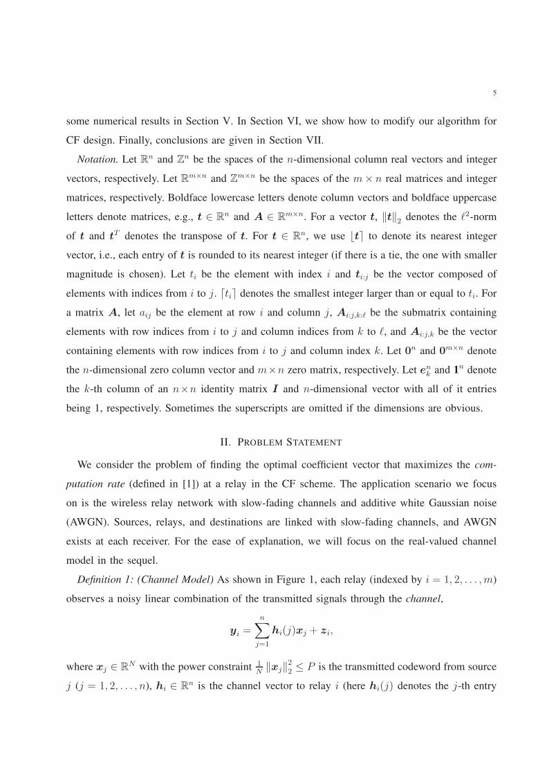
Definition 1: (Channel Model) As shown in Figure 1, each relay (indexed by i = 1, 2, . . . , m)

observes a noisy linear combination of the transmitted signals through the channel,

yi =n∑

j=1

hi(j)xj + zi,

where xj ∈ RN with the power constraint 1

N‖xj‖22 ≤ P is the transmitted codeword from source

j (j = 1, 2, . . . , n), hi ∈ Rn is the channel vector to relay i (here hi(j) denotes the j-th entry

6

of hi), zi ∈ RN is the noise vector with entries being i.i.d. Gaussian, i.e., zi ∼ N (0, I), and

yi is the signal received at relay i.

...

...

Sources

...

...

Relays Destination

Fig. 1. Channel Model

For relay i with the channel vector hi, let ai be the chosen coefficient vector, the computation

rate is calculated according to the following theorem [1].

Theorem 1: The computation rate at relay i is uniquely maximized by choosing the amplifying

factor as the MMSE coefficient, which results in a computation rate

R (hi,ai) =1

2log+

(

‖ai‖22 −P(

hTi ai

)2

1 + P ‖hi‖22

)−1

, (1)

where the log function is with respect to base 2 and log+(x) , max (log(x), 0).

Also, we define the optimal coefficient vector for a relay as below.

Definition 2: (The Optimal Coefficient Vector) The optimal coefficient vector a⋆i for a relay

with channel vector hi is the one that maximizes the computation rate,

a⋆i = arg max

ai∈Zn\0R (hi,ai) . (2)

The optimization problem (2) can be further formulated as the following problem [5]:

a⋆i = arg min

ai∈Zn\0aTi Giai, (3a)

Gi = I − P

1 + P ‖hi‖22hih

Ti . (3b)

7

Hereafter, we will focus on relay i, and thus ignore the subscript “i”, e.g., hi will be directly

written as h. In the next section, an efficient method to solve (3) based on sphere decoding will

be provided.

III. PROPOSED METHOD

Define the scaled channel vector t as

t =

√

P

1 + P ‖h‖22h. (4)

Then, (3) is equivalent to the following problem:

a⋆ = arg mina∈Zn\0

aTGa, (5a)

G , I − ttT . (5b)

Obviously, ‖t‖2 < 1 and G is symmetric positive definite. Throughout this paper, we assume

h 6= 0; otherwise, it is trivial.

The problem in (5) can be solved via the following two steps:

• First, for a given t, compute G and find its Cholesky factorization, i.e., find an upper

triangular matrix R such that G = RTR. Then (5) is equivalent to the following shortest

vector problem (SVP),

a⋆ = arg mina∈Zn\0

‖Ra‖2 . (6)

• Second, use a search algorithm, such as the LLL-aided Schnorr-Euchner search strategy

[17], to solve (6). We will explain the details later.

It is easy to see that for a given t, computing G costs O(n2) flops. Besides, it is well-known

that computing the Cholesky factorization of a general n×n matrix costs O(n3) flops. Moreover,

the complexity of the LLL-aided Schnorr-Euchner search strategy [17] for solving (6) may be

too high. Fortunately, we find out that it is possible to accelerate the aforementioned two steps

as follows:

• First, take advantage of the special structure of G in (5b) to compute its Cholesky factor-

ization and transform (5) to (6), but do not explicitly form G, the whole R and the SVP.

8

• Second, investigate the properties of a solution a∗ to (6) and take them into account to

modify the Schnorr-Euchner search strategy [17] to find a⋆.

Obviously, if a⋆ is a solution of (6), then −a⋆ is also a solution. For simplicity, we apply the

following restriction.

Restriction 1: Throughout this paper, we restrict the solution a⋆ to (6) such that tTa⋆ ≥ 0.

A. Transformation of the problem

To transform (5) to the SVP (6), we need to find the Cholesky factorization of G in (5b).

Besides the regular method, one can use the algorithm proposed in [18], which costs 2n2+O(n)

flops, to get the Cholesky factor R. However, the complexity can be further reduced. Also, to

analyze the complexity of our proposed search algorithm in Section IV, we need to know the

diagonal entries of R. In this subsection, we will take into account the special structure of G to

achieve this goal with only O(n) flops (we do not form the whole R explicitly. If the whole R

is needed for other applications, it costs n2/2+O(n) flops). Based on the diagonal entries of R

and by investigating their properties, we will also propose some conditions that can be checked

by O(n) flops, under which the optimal solution a⋆ can be obtained immediately without using

any search algorithm.

Our algorithm to find the Cholesky factor R of G in (5b) is based on the following theorem:

Theorem 2: The Cholesky factor R of G in (5b) is given by:

rij =

√

1−∑i

l=1 t2l

1−∑i−1

l=1 t2l, j = i

−titj√1−

∑i−1l=1 t2l

√1−

∑il=1 t

2l

, i < j ≤ n

, (7)

where 1 ≤ i ≤ n and denote∑0

1 · = 0.

Proof. To prove the theorem, we show any element of G is equal to the corresponding element

of RTR in the same position, i.e., by (5b), we would like to show

k∑

i=1

r2ik = 1− t2k, 1 ≤ k ≤ n, (8)

k∑

i=1

rikrij = −tktj, 1 ≤ k < j ≤ n. (9)

9

By (7), we have

k∑

i=1

r2ik = r2kk +

k−1∑

i=1

r2ik =1−∑k

l=1 t2l

1−∑k−1l=1 t2l

+

k−1∑

i=1

t2i t2k

(1−∑i−1l=1 t

2l )(1−

∑il=1 t

2l )

=1−∑k

l=1 t2l

1−∑k−1l=1 t2l

+ t2k

k−1∑

i=1

( 1

1−∑il=1 t

2l

− 1

1−∑i−1l=1 t

2l

)

=1−∑k

l=1 t2l

1−∑k−1l=1 t2l

+ t2k( 1

1−∑k−1l=1 t2l

− 1)

=1−∑k

l=1 t2l

1−∑k−1l=1 t2l

+t2k∑k−1

l=1 t2l

1−∑k−1l=1 t2l

= 1− t2k,

k∑

i=1

rikrij = rkkrkj +

k−1∑

i=1

rikrij =−tktj

1−∑k−1i=1 t

2i

+

k−1∑

i=1

t2i tktj

(1−∑i−1l=1 t

2l )(1−

∑il=1 t

2l )

=−tktj

1−∑k−1i=1 t2i

+ tktj

k−1∑

i=1

t2i

(1−∑i−1l=1 t

2l )(1−

∑il=1 t

2l )

=−tktj

1−∑k−1i=1 t2i

+ tktj( 1

1−∑k−1l=1 t2l

− 1)

=−tktj

1−∑k−1i=1 t

2i

+tktj

∑k−1i=1 t2i

1−∑k−1i=1 t

2i

= −tktj .

Thus, both (8) and (9) hold, completing the proof.

We can use Theorem 2 to design an efficient algorithm to find R. To simplify notation, we

introduce an (n+ 1)-dimensional vector variable f . Let

f0 = 1, fi = 1−i∑

l=1

t2l , 1 ≤ i ≤ n. (10)

Then by (7), we have

rii =√

fi/fi−1, 1 ≤ i ≤ n,

Ri,i+1:n = (−ti/√

fifi−1)tTi+1:n, 1 ≤ i < n.

Note that Ri,i+1:n is a scaled tTi+1:n.

After getting R, we will modify the Schnorr-Euchner search algorithm to solve (6). Later

we will see that it is not necessary to form R explicitly (we will give more details to explain

this in the last subsection of this section), i.e, we do not need to compute the multiplication of

−ti/√

fifi−1 and ti+1:n. Thus, the complexity of obtaining R is O(n) flops.

By (7), it is easy to see that R has the following properties which are useful to analyze the

complexity of our proposed search algorithm.

10

Theorem 3: For 1 ≤ k ≤ n, the following inequalities hold:

√

√

√

√1−k∑

i=1

t2i ≤ rkk ≤√

1− t2k, (11)

n∏

i=k

rii =

√

1− ‖t‖22√

1−∑k−1i=1 t

2i

≥√

1− ‖t‖22. (12)

Proof. The first inequality in (11) follows direct from (7) and the basic fact that 1−∑i−1l=1 t

2l ≤ 1

for 1 ≤ i ≤ n (recall that we define∑0

l=1 · = 0).

The second inequality in (11) follows direct from (8).

The equality in (12) follows direct from (7) and the inequality in (12) follows from the basic

fact that 1−∑i−1l=1 t

2l ≤ 1 for 1 ≤ i ≤ n.

By Theorem 2, we have the following interesting result, which can be used to describe the

geometry of the search space later.

Theorem 4: For 1 ≤ i < j ≤ n, the eigenvalues of RTi:j,i:jRi:j,i:j are fj/fi−1 (f is defined in

(10)) and 1 with algebraic multiplicity j − i.

Proof. We first prove

RTi:n,i:nRi:n,i:n = In−i+1 −

ti:n√

fi−1

tTi:n√

fi−1

. (13)

If i = 1, then by Theorem 2 and (10), (13) holds. So we only need to prove it holds for i > 1.

By Theorem 2, we have

RT1:i−1,1:i−1 0

RT1:i−1,i:n RT

i:n,i:n

R1:i−1,1:i−1 R1:i−1,i:n

0 Ri:n,i:n

=

I i−1 0

0 In−i+1

−

t1:i−1tT1:i−1 t1:i−1t

Ti:n

ti:ntT1:i−1 ti:nt

Ti:n

.

The right bottom parts of both sides are the same, thus,

RTi:n,i:nRi:n,i:n = In−i+1 − ti:nt

Ti:n −RT

1:i−1,i:nR1:i−1,i:n.

And by Theorem 2, we have

R1:i−1,i:n =

(

ti:n

[

−t1√f0f1

−t2√f1f2

. . . −ti−1√fi−2fi−1

])T

.

11

Thus, we obtain

RTi:n,i:nRi:n,i:n = In−i+1 − (1 +

i−1∑

k=1

t2kfkfk−1

)ti:ntTi:n.

By (10),t2k

fkfk−1=

1

fk− 1

fk−1.

Therefore,

RTi:n,i:nRi:n,i:n = In−i+1 −

ti:n√

fi−1

tTi:n√

fi−1

,

i.e., (13) holds. From (13), we can get

RTi:j,i:jRi:j,i:j = Ij−i+1 −

ti:j√

fi−1

tTi:j√

fi−1

.

Thus, the eigenvalues of RTi:j,i:jRi:j,i:j are 1’s and 1−

∑jk=i t

2k

fi−1=

fjfi−1

.

Generally speaking, after getting R, a search algorithm should be used to find the solution

a⋆ to (6). Theorem 2 gives the closed-form expression of R, so a natural question is whether

there exist some easily-checked conditions, under which the optimal solution a⋆ can be obtained

without using any search algorithm? In the following, we will answer this question.

Theorem 5: The optimal solution a⋆ satisfies

‖Ra⋆‖2 ≥ min1≤i≤n

√

√

√

√

1−∑ij=1 t

2j

1−∑i−1j=1 t

2j

≥√

1− ‖t‖22. (14)

Furthermore, if we have

t2i ≤ t21(1−i−1∑

j=1

t2j ), i = 2, 3 . . . , n, (15)

then e1 is a solution to (6).

Proof. The first inequality in (14) follows directly from (7) and

‖Ra⋆‖2 ≥ min1≤i≤n

rii, (16)

which was given in [19, pp.99].

12

By the first inequality in (11),

min1≤i≤n

rii ≥√

1− ‖t‖22.

Therefore, the second inequality in (14) follows.

In the following, we prove the second part. If for some 1 ≤ i ≤ n,

t2i ≤ t21(1−i−1∑

j=1

t2j).

Then,

i∑

j=1

t2j −i−1∑

j=1

t2j ≤ t21(1−i−1∑

j=1

t2j ).

Thus,

1−i∑

j=1

t2j ≥ (1−i−1∑

j=1

t2j )− t21(1−i−1∑

j=1

t2j ).

Equivalently, we have√

√

√

√

1−∑ij=1 t

2j

1−∑i−1j=1 t

2j

≥√

1− t21.

Thus, from (15) holds, we have

min1≤i≤n

√

√

√

√

1−∑ij=1 t

2j

1−∑i−1j=1 t

2j

=√

1− t21.

Therefore, the first inequality in (14) becomes an equality with a⋆ = e1, so e1 is a solution to

(6).

It is easy to see that (15) can be checked by O(n) flops.

Remark 1: From (5b), we can see that

min1≤i≤n

eTi Gei = min

1≤i≤n(‖ei‖2 − (eT

i t)2) = min

1≤i≤n(1− t2i ).

Thus, if max1≤i≤n

|ti| 6= |t1|, then e1 cannot be an optimal solution. Thus, (15) does not hold.

However, we can order the entries of t such that after the ordering, max1≤i≤n

|ti| = |t1|. Clearly,

doing this can increase the probability of (15) holds. And ej with j satisfying max1≤i≤n |ti| = |tj|

13

( here t is the vector before using the transformation) is an optimal solution. Naturally, it is

interesting to know how often does (15) hold? We will do some simulations for this in the end

of next subsection.

B. Reordering the entries of t

After getting (6), a search algorithm, such as the Schnorr-Euchner search strategy [17] can be

used to solve it, i.e., finding the shortest nonzero vector of the lattice L(R), which is defined

by

L(R) = Rz|z ∈ Zn.

The columns of R form a basis of L(R) (note that the basis of a lattice is not necessary an

upper triangular matrix, but it must be a full column rank matrix). For any n ≥ 2, L(R) has

infinity many bases and any of two are connected by a unimodular matrix Z, i.e., Z ∈ Zn×n and

det(Z) = ±1. Specifically, for each given lattice basis matrix R ∈ Rm×n, RZ is also a basis

matrix of L(R) if and only if Z is unimodular, see, e.g., [20]. The process of selecting a good

basis for a given lattice, given some criterion, is called lattice reduction. In many applications,

it is advantageous if the basis vectors are short and close to be orthogonal [20]. For more than a

century, lattice reduction have been investigated by many people and several types of reductions

have been proposed, including the KZ reduction [21] (an efficient KZ reduction algorithm can

be found in [22]), the Minkowski reduction [23] (an efficient Minkowski reduction algorithm

can be found in [24]), the LLL reduction [10] and Seysen’s reduction [25] etc.

For efficiency, lattice reduction for R in (6) is usually used to strive for

r11 ≤ r22 ≤ . . . ≤ rnn (17)

to accelerate searching. Notice that (15) may not be achievable. For more details on why (17)

is desirable for, readers are referred to, e.g., [20] and [26].

The LLL reduction [10] is a commonly used reduction method to strive for (17). However, for

this application, it has two main drawbacks. First, its complexity is high. In fact, it was shown

in [11] that in the MIMO context, the worst-case complexity is not even finite. For more details,

see, e.g., [10], [27] and [12]. Also, from the simulation results in Section V, we will see that the

complexity of the LLL reduction is even higher than that of our proposed algorithm. Second, it

14

may destroy the structure of R and some properties of the optimal solution a⋆ to the reduced

problem (we will explain this in the latter part of this subsection). In this subsection, we will

propose a method to strive for (17) without the above shortcomings.

From (7), to strive for (17), we permute the entries of t. To make r11 as small as possible,

we permute t such that |t1| is the largest. Suppose that tj, 1 ≤ j ≤ i have been fixed, then from

(7), rjj, 1 ≤ j ≤ i are fixed. To make rj+1,j+1 as small as possible, we permute the entries of

tj , i+ 1 ≤ j ≤ n such that |tj+1| is the largest. So after the permutations we have

|t1| ≥ |t2| ≥ . . . ≥ |tn|. (18)

Here we want to point out the above idea of reordering the entries of t is actually the same

as that of SQRD [28], a column reordering strategy for a general matrix in the box-constrained

integer least squares (BILS) problem [29], [30]. It is interesting to note that if we use the idea

of V-BLAST [31], another column reordering strategy used in solving BILS problems [32], we

will get the same ordering of t. In fact, by (7),

r2nn =1− ‖t‖22

1− ‖t‖22 + t2n.

Thus, to make rnn as large as possible, we need to permute t such that |tn| is the smallest.

Suppose that tj , i+ 1 ≤ j ≤ n have been fixed, then from (7), rjj, i+ 1 ≤ j ≤ n are fixed. By

(7),

r2ii =1− ‖t‖22 +

∑nj=i+1 t

2j

1− ‖t‖22 +∑n

j=i+1 t2j + t2i

.

Thus, to make rjj as large as possible, we permute the entries of tj , 1 ≤ j ≤ i such that |ti| is

the smallest. So after the permutations we also have (18).

To make the search process faster, we also want to make ti ≥ 0 for 1 ≤ i ≤ n. This can easily

be done. In fact, when we determine the i-th entry of t in the permutation process, we can use

a sign permutation matrix so that the new i-th entry is nonnegative. Thus, eventually we have

t1 ≥ t2 ≥ . . . ≥ tn ≥ 0. (19)

The above process can be described mathematically as follows. For any given t, it is easy to

15

find a signed permutation matrix Z ∈ Zn×n such that t = Zt satisfying:

t1 ≥ t2 ≥ . . . ≥ tn ≥ 0.

This transformation is a sorting process and the complexity is O(n log(n)), see [13] for more

details. Note that ZZT = I . Then, with a = Za, the optimization problem (5) can be

transformed to

a⋆ = mina∈Zn\0

aT Ga,

G , I − ttT.

Obviously a⋆ = ZT a⋆.

Therefore, for the sake of convenience, in our later analysis, we assume t satisfies (19).

Except speeding up the search, ordering the entries of t like in (19) has another important

effect. By the results in [6] and [13], if (19) holds, we can find a solution a⋆ to (6) such that

a⋆1 ≥ a⋆2 ≥ . . . ≥ a⋆n ≥ 0. (20)

The order of the elements of the solution a∗ in (20) is a key property of the solution we

restricted for (6). It has been used in [13] to find a suboptimal solution to (6), but only the

property that ai ≥ 0, 1 ≤ i ≤ n has been used in [6] to solve (6). In this paper, we will take

full advantage of it in designing the search algorithm. Note that, if the LLL reduction is used

for reducing R in (6), then (20) may not hold, which is the second drawback of using the LLL

reduction in striving for (19). The motivation for reordering the entries of t in [6] and [13] is

to obtain the property (20), which was (partially) used in their methods. Here we gave another

motivation from the search point of view.

Under (19) and Theorem 2, we have the following interesting results:

Theorem 6: If (19) holds, then for 1 ≤ i ≤ n− 1

rii ≤ ‖Ri:i+1,i+1‖2 ≤ ‖Ri:i+2,i+2‖2 ≤ . . . ≤ ‖Ri:n,n‖2 (21)

16

Proof. By (7), for 1 ≤ i < j ≤ n,

‖Ri:j,j‖2 =j−1∑

k=i

r2kj + r2jj =

j−1∑

k=i

t2kt2j

(1−∑k−1l=1 t2l )(1−

∑kl=1 t

2l )

+1−∑j

l=1 t2l

1−∑j−1l=1 t

2l

=t2j

1−∑j−1l=1 t

2l

− t2j

1−∑i−1l=1 t

2l

+1−∑j

l=1 t2l

1−∑j−1l=1 t

2l

= 1− t2j

1−∑i−1l=1 t

2l

.

By the aforementioned equations, (7) and (19), it is easy to see that (21) holds.

In the following, we do some simulations to show how often (15) hold? For each n and P ,

we randomly generate 10000 realizations of h. Then, we compute t by (4) and transform it

such that (19) holds. Tables I and II respectively show the total number of cases over 10000

realizations that (15) holds for n from 2 to 16 with step 2 and n from 100 to 800 with step 100.

From Tables I and II, we can see that, (15) holds with a high probability when both n and P

are small and with a very low probability when both n and P are very large.

TABLE I

NUMBER OF e1 BEING THE OPTIMAL SOLUTION OVER 10000 REALIZATIONS OF h

Pn

2 4 6 8 10 12 14 16

P=0 db 8617 6172 4948 4255 3778 3641 3486 3468

P=10 db 6148 2767 1728 1222 1025 881 790 731

P=20 db 3903 944 413 223 146 101 70 59

TABLE II

NUMBER OF e1 BEING THE OPTIMAL SOLUTION OVER 10000 REALIZATIONS OF h

Pn

100 200 300 400 500 600 700 800

P=0 db 4837 4833 4568 4065 3540 3324 2866 2589

P=10 db 196 64 35 15 9 5 9 2

P=20 db 0 0 0 0 0 0 0 0

C. Schnorr-Euchner search algorithm

We first introduce a depth-first tree search algorithm: the Schnorr-Euchner search algorithm

[17], [20], a variation of the Fincke-Pohst search strategy [4], to solve a general SVP, which has

the form of (6). Note that, the Schnorr-Euchner algorithm is generally more efficient than the

Fincke-Pohst, see, e.g., [20]. Then we modify it by using the properties of R and the optimal

solution a⋆ to make the search process faster.

17

Let the optimal solution be within the following hyper-ellipsoid:

‖Ra‖22 < β2, (22)

where β is a constant. Define

dn = 0, dk = − 1

rkk

n∑

j=k+1

rkjaj , k = n− 1, . . . , 1. (23)

Then (22) can be written as∑n

i=1 r2ii(ai − di)

2 < β2, which is equivalent to

r2kk(ak − dk)2 < β2 −

n∑

j=k+1

r2jj(ai − dj)2 (24)

for k = n, n− 1, . . . , 1, where k is called the level index and∑n

j=n+1 · = 0.

Based on (24), the Schnorr-Euchner search algorithm can be described as follows. First we

set the initial β = ∞, and for k = n, n − 1, . . . , 1, we compute dk by (23) and set ak = ⌊dk⌉,

leading to ak = 0, for which (24) holds. So we obtain an integer vector a = 0. Since the optimal

solution a⋆ is a nonzero vector, we need to update a. Specifically, we set a1 as the next closest

integer to d1. Note that (24) with k = 1 holds for the updated a. Then, we store this updated

a and set β = ‖Ra‖2. After this, we try to find an integer vector within the new ellipsoid by

updating the latest found a. Obviously, we cannot update only its first entry a1, since we cannot

find any new integer a1 that satisfies (24) with k = 1, which is now an equality for the current

a. Thus we move up to level 2 to try to update a2 by choosing it being the next nearest integer

to d2. If it satisfies (24) with k = 2, we move down to level 1 to update a1 by computing d1 (see

(23)) and setting a1 = ⌊d1⌉ and then checking if (24) with k = 1 holds and so on; otherwise

we move up to level 3 to try to update a3, and so on. Finally, when we fail to find a new value

for an to satisfy (24) with k = n, the search process stops and the latest found integer vector

is the optimal solution a⋆ we seek. This is a depth-first tree search. For more details, see, e.g.,

[20] and [29].

We summarize the search process in Algorithm 1, where

sgn(x) =

1, x ≥ 0

−1, x < 0. (25)

18

Algorithm 1: Schnorr-Euchner search algorithm

Input: A nonsingular upper triangular matrix R ∈ Rn×n

Output: A solution a⋆ to the SVP in (6)

1) (Initialization) Set k = n, β = +∞.

2) Compute dk by using (23), set ak = ⌊dk⌉ and sk = sgn(dk − ak) (see (25)).

3) (Main Step) If the inequality in (24) does not hold, then go to Step 4. Else if k > 1, set

k = k − 1 and go to Step 2. Else (k = 1), go to Step 5.

4) (Outside ellipsoid) If k = n, terminate. Else, set k = k + 1 and go to Step 6.

5) (A valid point is found) If a 6= 0, then save a⋆ = a, set β = ‖Ra‖2 and k = k + 1.

6) (Enumeration at level k) Set ak = ak + sk, sk = −sk−sgn(sk) and go to Step 3.

D. Modified Schnorr-Euchner search algorithm

In the following we make some comments to Algorithm 1 and make some modifications. It

is easy to see that, the first nonzero integer vector encountered by Algorithm 2 is e1 and the

corresponding search radius is

β = |r11| =√

1− t21. (26)

Note that reordering the entries of t that makes (19) hold gives the smallest β among any other

orderings. This shows one of the benefits of the reordering leading to (19). Also from (21), the

reordering gives

β = |r11| = min1≤i≤n

‖R1:i,i‖2 ,

which implies e1 is better than any other ei for i = 2, . . . , n, as the former corresponds to the

smallest residual. In the modified algorithm, we just start with β given by (26).

In Section III-A, we mentioned that it is not necessary to form the entries of R explicitly; in

the following, we show how to compute rkk and dk for 1 ≤ k ≤ n, which are needed in (24).

By (7) and (10), we have

r2kk = fk/fk−1, 1 ≤ k ≤ n. (27)

In the modified algorithm, we will use a n-dimensional vector q to store r2kk, i.e., let qk = r2kk.

By (7), (10) and (23),

dk =tkfk

n∑

j=k+1

tjaj.

Thus, for computational efficiency, we introduce an (n+1)-dimensional vector p with pn+1 = 0

19

to store some computed quantities. Specifically, after ak, 1 ≤ k ≤ n is chosen in the search

process, we assume

pk = pk+1 + tkak, 1 ≤ k ≤ n, (28)

which explains why pn+1 = 0. Therefore, we have

dk =tkpk+1

fk, 1 ≤ k ≤ n. (29)

Now we make the main modification to Algorithm 2 by using the property of a⋆ in (20). Note

that in the search process of finding an integer point a in the hyper-ellipsoid, the entries of a

are determined in the following order: an, an−1, . . . , a1. When we enumerate candidates for an

at level n, we will only enumerate the non-negative integers. When we enumerate candidates

for ak at level k (note that at this point, an, an−1, . . . , ak+1 have been chosen), we will only

enumerate those greater than or equal to ak+1. By doing these we can prune a lot of nodes from

the search tree to make the search process much faster.

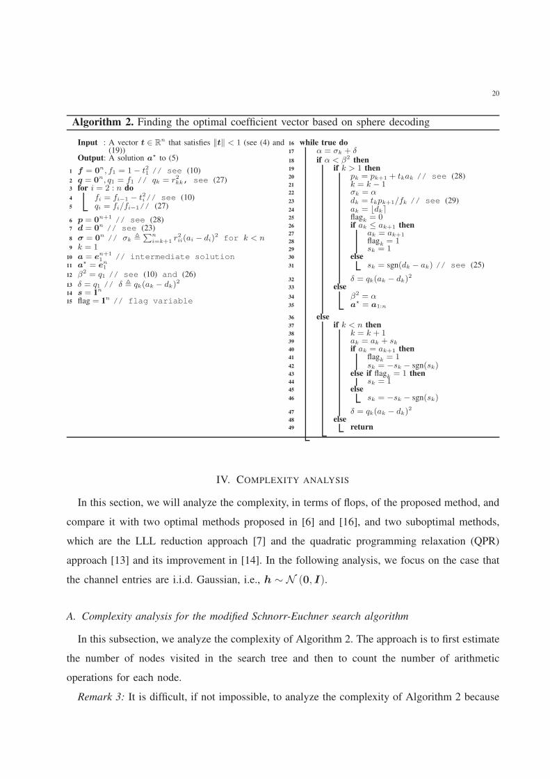
For the users to implement the algorithm easily and for our later complexity analysis, we

provide the pseudo code of the modified algorithm in Algorithm 2.

Here we make a few comments to Algorithm 2. To unify the enumeration strategies for level

n and for any lower level, we set a to be an (n + 1)-dimensional vector with an+1 ≡ 0, so

that ak ≥ ak+1 holds for k = n. To avoid enumerating any integer smaller than ak+1 at level k,

we introduced a flag variable “flag” in the algorithm to indicate whether the enumeration has

reached the lower bound ak+1 for 1 ≤ k ≤ n. In the algorithm sk is the difference between the

next integer candidate for ak and the current value of ak and it is used to get the next integer

candidate for ak.

Remark 2: By Theorem 5, if (15) holds, then e1 is the solution. Therefore, before using the

Modified Schnorr-Euchner search algorithm to find the optimal solution, we can test whether

(15) holds. If it holds, then return e1, otherwise, we use the search algorithm to find the optimal

solution. This can usually further improve the efficiency of the algorithm, especially when n or

P is small. But from Table II, we can see this case occurs in a very low probability when both

n and P are very large. Thus, for simplicity, we do not incorporate it in Algorithm 2.

20

Algorithm 2. Finding the optimal coefficient vector based on sphere decoding

Input : A vector t ∈ Rn that satisfies ‖t‖ < 1 (see (4) and

(19))Output: A solution a⋆ to (5)

1 f = 0n, f1 = 1− t21 // see (10)

2 q = 0n, q1 = f1 // qk = r2kk, see (27)

3 for i = 2 : n do

4 fi = fi−1 − t2i// see (10)5 qi = fi/fi−1// (27)

6 p = 0n+1

// see (28)7 d = 0

n// see (23)

8 σ = 0n // σk ,

∑ni=k+1 r

2ii(ai − di)

2 for k < n9 k = 1

10 a = en+11 // intermediate solution

11 a⋆ = en1

12 β2 = q1 // see (10) and (26)

13 δ = q1 // δ , qk(ak − dk)2

14 s = 1n

15 flag = 1n// flag variable

16 while true do17 α = σk + δ18 if α < β2 then19 if k > 1 then20 pk = pk+1 + tkak // see (28)21 k = k − 122 σk = α23 dk = tkpk+1/fk // see (29)24 ak = ⌊dk⌉25 flagk = 026 if ak ≤ ak+1 then27 ak = ak+128 flagk = 129 sk = 130 else31 sk = sgn(dk − ak) // see (25)

32 δ = qk(ak − dk)2

33 else

34 β2 = α35 a⋆ = a1:n

36 else37 if k < n then38 k = k + 139 ak = ak + sk40 if ak = ak+1 then41 flagk = 142 sk = −sk − sgn(sk)43 else if flagk = 1 then44 sk = 145 else46 sk = −sk − sgn(sk)

47 δ = qk(ak − dk)2

48 else49 return

IV. COMPLEXITY ANALYSIS

In this section, we will analyze the complexity, in terms of flops, of the proposed method, and

compare it with two optimal methods proposed in [6] and [16], and two suboptimal methods,

which are the LLL reduction approach [7] and the quadratic programming relaxation (QPR)

approach [13] and its improvement in [14]. In the following analysis, we focus on the case that

the channel entries are i.i.d. Gaussian, i.e., h ∼ N (0, I).

A. Complexity analysis for the modified Schnorr-Euchner search algorithm

In this subsection, we analyze the complexity of Algorithm 2. The approach is to first estimate

the number of nodes visited in the search tree and then to count the number of arithmetic

operations for each node.

Remark 3: It is difficult, if not impossible, to analyze the complexity of Algorithm 2 because

21

the search radius β changes in the search process. Thus, we assume that the search radius β

keeps unchanged in our following analysis to obtain an estimate of the upper bound on the

complexity of Algorithm 2.

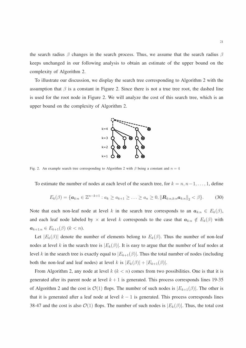
To illustrate our discussion, we display the search tree corresponding to Algorithm 2 with the

assumption that β is a constant in Figure 2. Since there is not a true tree root, the dashed line

is used for the root node in Figure 2. We will analyze the cost of this search tree, which is an

upper bound on the complexity of Algorithm 2.

k=4

k=3

k=2

k=1

Fig. 2. An example search tree corresponding to Algorithm 2 with β being a constant and n = 4

To estimate the number of nodes at each level of the search tree, for k = n, n−1, . . . , 1, define

Ek(β) = ak:n ∈ Zn−k+1 : ak ≥ ak+1 ≥ . . . ≥ an ≥ 0, ‖Rk:n,k:nak:n‖2 < β. (30)

Note that each non-leaf node at level k in the search tree corresponds to an ak:n ∈ Ek(β),

and each leaf node labeled by × at level k corresponds to the case that ak:n /∈ Ek(β) with

ak+1:n ∈ Ek+1(β) (k < n).

Let |Ek(β)| denote the number of elements belong to Ek(β). Thus the number of non-leaf

nodes at level k in the search tree is |Ek(β)|. It is easy to argue that the number of leaf nodes at

level k in the search tree is exactly equal to |Ek+1(β)|. Thus the total number of nodes (including

both the non-leaf and leaf nodes) at level k is |Ek(β)|+ |Ek+1(β)|.From Algorithm 2, any node at level k (k < n) comes from two possibilities. One is that it is

generated after its parent node at level k+1 is generated. This process corresponds lines 19-35

of Algorithm 2 and the cost is O(1) flops. The number of such nodes is |Ek+1(β)|. The other is

that it is generated after a leaf node at level k − 1 is generated. This process corresponds lines

38-47 and the cost is also O(1) flops. The number of such nodes is |Ek(β)|. Thus, the total cost

22

for generating all nodes at level k is

ck = (|Ek(β)|+ |Ek+1(β)|)O(1), (31)

where we denote |En+1(β)| = 0. Let C(n) denote the total cost of the search tree, then, by (31),

we obtain

C(n) =

n∑

k=1

ck = O(1)

n∑

k=1

|Ek(β)|. (32)

Obviously, |En(β)| ≤ ⌈β/rnn⌉. However, it is hard to rigorously compute or estimate |Ek(β)|since the inequalities are involved in (30), so for k = 1, 2, . . . , n, we define supersets:

Fk(β) = ak:n ∈ Zn−k+1 : ‖Rk:n,k:nak:n‖ < β, (33)

where β is the initial search radius used in Algorithm 2 (see (26)).

Let |Fk(β)| denote the number of elements belong to Fk(β). Obviously, we have

|Ek(β)| ≤ |Fk(β)|. (34)

We apply the so-called Gaussian heuristic, which is widely used in the complexity analysis of

sphere decoding methods (see, e.g., [33], [34], [20], [35]), to estimate |Fk(β)|. This method

approximates |Fk(β)| by the volume of the hyper-ellipsoid ‖Rk:n,k:nak:n‖2 < β, namely,

|Fk(β)| ≈βn−k+1

∏ni=k rii

Vn−k+1, (35)

where Vn−k+1 denotes the volume of an (n− k + 1)-dimensional unit Euclidean ball, i.e.,

Vn−k+1 =π(n−k+1)/2

Γ((n− k + 1)/2 + 1)(36)

with Γ being the Gamma function.

By (12) and (26), we have

βn−k+1

∏ni=k rii

≤ (1−∑k−1i=1 t

2i )

1/2(1− t21)(n−k+1)/2

√

1− ‖t‖22≤ 1√

1− ‖t‖22. (37)

Since

Γ(n− k + 1

2+ 1) =

(n−k+12

)! if n− k is odd

√π(n−k+1)!!

2(n−k)/2+1 if n− k is even

,

23

where (n− k + 1)!! = 1× 3× 5× · · · × (n− k + 1), from (36), we have

Vn−k+1 =

π(n−k+1)/2

(n−k+12

)!if n− k is odd

2(2π)(n−k)/2

(n−k+1)!!if n− k is even

. (38)

By (38), it is not hard to see that limk 7→∞ Vk = 0. Therefore, by (37), instead of using (35), we

only need the following approximation, which is weaker than the Gaussian heuristic,

|Fk(β)| /1

√

1− ‖t‖22maxVn−k+1, 1. (39)

By direct calculation, we have V13 = 0.9106, V14 = 0.5993. By (38), obviously, Vi is decreasing

with i ≥ 13. Thus, from the aforementioned equation, we obtain Vi ≤ 1, ∀ i ≥ 13. By direct

calculation, we have max1≤j≤12 Vj = V5 = 5.2638. Therefore, combining with (32), (34) and

(39), we obtain (recall that C(n) is the total cost of the search tree)

C(n) /O(n)

√

1− ‖t‖22. (40)

By (4), we have

1√

1− ‖t‖22=

1√

1− P‖h‖221+P‖h‖22

=√

1 + P‖h‖22.

Thus, by (40), we obtain

C(n) / O(n)√

1 + P‖h‖22. (41)

In the following, we do some simulations to support that (41) holds for general n and h in (4).

From (32), we only need to show∑n

k=1 |Ek(β)| / O(n)√

1 + P‖h‖22. We consider the case

that the channel vector h ∼ N (0, I). For each pair of n and P , we randomly generate 10000

realizations of h.

Table III displays the average and largest ratios of∑n

k=1 |Ek(β)| to n√

1 + P‖h‖22 over 10000

samples. “AR” and “LR” in Table III respectively denote average and largest ratio. From Table

III, we can see that∑n

k=1 |Ek(β)| < 2n√

1 + P‖h‖22 in all the tests. Note that the number

of nodes searched by Algorithm 2 can not be larger than∑n

k=1 |Ek(β)| because the radius β

reduces whenever a valid integer vector is found in the search process.

24

TABLE III

AVERAGE AND LARGEST RATIOS (AR AND LR) OF∑n

k=1 |Ek(β)| TO n√

1 + P‖h‖22 OVER 10000 REALIZATIONS OF h

nP

P = 0 dB P = 20 dB P = 40 dB

AR LR AR LR AR LR

2 0.4241 1.4747 0.3032 1.3399 0.3178 0.9292

4 0.5259 1.7803 0.4273 1.3123 0.4401 1.4314

8 0.4408 1.2875 0.4040 1.2632 0.4253 1.5001

16 0.3204 0.9109 0.1813 0.5917 0.1887 0.6826

32 0.2205 0.6348 0.0610 0.1770 0.0509 0.2033

64 0.1471 0.3783 0.0265 0.0602 0.0127 0.0394

102 0.1143 0.2937 0.0183 0.0338 0.0054 0.0154

103 0.0381 0.0567 0.0048 0.0063 0.0005 0.0006

104 0.0129 0.0151 0.0014 0.0016 0.0001 0.0002

105 0.0040 0.0043 0.0004 0.0004 0.0000 0.0000

In the following, we would like to investigate the expected value of C(n) when the entries

of h are independent and identically follow normal distribution N (0, 1). It is easy to see that

‖h‖22 follows the chi-squared distribution χ2(n). Therefore, E[‖h‖22] = n. Since√1 + Px is a

concave function of x, by Jensen’s Inequality,

E

[

√

1 + P ‖h‖22]

≤√

1 + PE[

‖h‖22]

=√1 + nP . (42)

Therefore, by (41) and (42), the estimated average complexity of Algorithm 2 is O(n1.5P 0.5) flops.

B. Comparison of the complexity of the proposed method with other methods

It is easy to see that, for any given h, computing t by (4) costs O(n) flops. And for any

fixed t, transform it such that (19) holds costs O(n log(n)) flops. Since the total complexity of

Algorithm 2 is around O(n1.5P 0.5) flops, the total complexity of the whole method is estimated

to be O(n1.5P 0.5) flops for the test cases.

The complexity of the QPR in [13] and [14] is O(n3) and O(n1.5P 0.5) flops, respectively. The

method based on LLL lattice reduction [7] uses the regular method, costing O(n3), to obtain the

Cholesky factor R. The optimal method proposed in [6] needs to find the inverse of n matrices

and solving n linear equations with the dimensions from 1 to n, so its complexity is higher than

O(n3). The complexity of the optimal method proposed in [16] is O(n2.5P 0.5) flops. Therefore,

it is expected that our optimal algorithm is faster than the LLL reduction based method, the

QPR in [13] and the two optimal methods proposed in [7] and [16], and faster than or has more

or less the same speed as the QPR in [14].

25

V. NUMERICAL SIMULATIONS

In this section, we present the numerical results to demonstrate the effectiveness and efficiency

of our new method. We consider the case that the entries of the channel vector h ∈ Rn are i.i.d.

Gaussian, i.e., h ∼ N (0, I). The dimension n of h ranges from 2 to 16. For a given n, we

randomly generate 10000 realizations of h for each P from 0 dB to 20 dB with the step length

1 dB, and apply different methods to calculate the corresponding computation rates. To compare

the effectiveness of different methods, we compute the average computation rates; to compare

the efficiency, we record the running time.

The methods considered include our new method called the improved sphere decoding (ISD)

method, the branch-and-bound (BnB) algorithm in [6], the optimal method proposed in [16] (to

be called SG named after the authors), the method based on LLL lattice reduction algorithm

[7] (to be called LLL), and the quadratic programming relaxation (QPR) approach [14]. The

quality-complexity tradeoff factor δ in the LLL method is set as 0.75. A larger δ (1/4 < δ ≤ 1)

can give a higher rate, but the running time will increase drastically as δ increases. The upper

bound of the number of real-valued approximations, Ku, in the QPR method is set according to

the criterion proposed in [14]. Exact values of Ku used in the simulations are listed in Table IV.

0 2 4 6 8 10 12 14 16 18 200.4

0.6

0.8

1

1.2

1.4

1.6

P (dB)

Avera

ge c

om

puta

tion r

ate

(bits/c

hannel use)

ISD

SG

BnB

LLL, δ=0.75

QPR, Ku=4

(a) n = 4

0 2 4 6 8 10 12 14 16 18 200.3

0.4

0.5

0.6

0.7

0.8

P (dB)

Avera

ge c

om

puta

tion r

ate

(bits/c

hannel use)

ISD

SG

BnB

LLL, δ=0.75

QPR, Ku=6

(b) n = 8

0 2 4 6 8 10 12 14 16 18 200.1

0.15

0.2

0.25

0.3

P (dB)

Avera

ge c

om

puta

tion r

ate

(bits/c

hannel use)

ISD

SG

BnB

LLL, δ=0.75

QPR, Ku=4

(c) n = 16

Fig. 3. Average computation rates by different methods.

TABLE IV

THE UPPER BOUND OF THE NUMBER OF REAL-VALUED APPROXIMATIONS IN QPR METHOD

n 2 3 4 5 6 7 8 9 10 11 12 13 14 15 16

Ku 2 3 4 5 5 5 6 6 6 6 7 6 6 6 4

We first compare the average computation rates. Figures 3(a), 3(b), 3(c) show the average

26

computation rates over 10000 samples with the dimension n being 4, 8, and 16, respectively.

The ISD method, the BnB method and the SG methods are optimal. As expected, numerical

results show that they always provide the highest computation rate. The corresponding curves of

these three methods in Figure 3 exactly overlap with each other. The QPR method and the LLL

based method provide rates close to that of the optimal methods. However, as the dimension

increases, their performance degrade.

2 4 6 8 10 12 14 1610

−1

100

101

102

n

Runnin

g tim

e for

10000 s

am

ple

s (

seconds)

ISD

SG

BnB

LLL, δ=0.75

QPR

(a) P = 0 dB

2 4 6 8 10 12 14 1610

−1

100

101

102

103

n

Runnin

g tim

e for

10000 s

am

ple

s (

seconds)

ISD

SG

BnB

LLL, δ=0.75

QPR

(b) P = 10 dB

2 4 6 8 10 12 14 1610

−1

100

101

102

103

n

Runnin

g tim

e for

10000 s

am

ple

s (

seconds)

ISD

SG

BnB

LLL, δ=0.75

QPR

(c) P = 20 dB

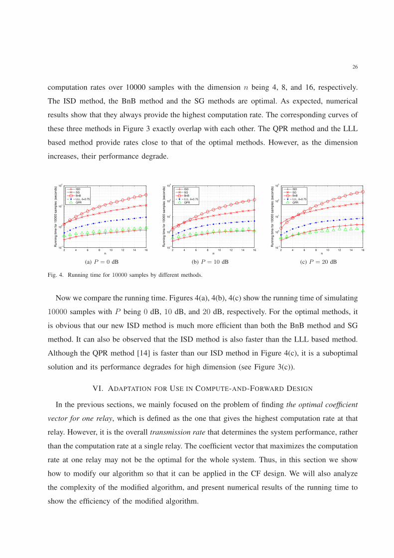
Fig. 4. Running time for 10000 samples by different methods.

Now we compare the running time. Figures 4(a), 4(b), 4(c) show the running time of simulating

10000 samples with P being 0 dB, 10 dB, and 20 dB, respectively. For the optimal methods, it

is obvious that our new ISD method is much more efficient than both the BnB method and SG

method. It can also be observed that the ISD method is also faster than the LLL based method.

Although the QPR method [14] is faster than our ISD method in Figure 4(c), it is a suboptimal

solution and its performance degrades for high dimension (see Figure 3(c)).

VI. ADAPTATION FOR USE IN COMPUTE-AND-FORWARD DESIGN

In the previous sections, we mainly focused on the problem of finding the optimal coefficient

vector for one relay, which is defined as the one that gives the highest computation rate at that

relay. However, it is the overall transmission rate that determines the system performance, rather

than the computation rate at a single relay. The coefficient vector that maximizes the computation

rate at one relay may not be the optimal for the whole system. Thus, in this section we show

how to modify our algorithm so that it can be applied in the CF design. We will also analyze

the complexity of the modified algorithm, and present numerical results of the running time to

show the efficiency of the modified algorithm.

27

A. Adapting the proposed algorithm

In this subsection, we show how to adapt our algorithm for use in CF design.

The transmission rate is the minimum computation rate over all relays if the coefficient

matrix, which is formed by the coefficient vectors at relays, is full column rank; and it is 0 if

the coefficient matrix has rank deficiency [1]. One naive strategy is to let each relay choose the

coefficient vector that maximizes the computation rate. However, it has been shown in [5] to be

inherently suboptimal since there is a high probability that the formed coefficient matrix is not

full rank, especially for low SNR. Instead, we can adopt the strategy (named “Wei-Chen” after

the authors) proposed in [5]: 1) Each relay searches a list of candidate coefficient vectors, and

then forwards the list to the destination; 2) The destination does a search based on the received

lists, and finds a good set of coefficient vectors that can form a full rank coefficient matrix, and

then sends back to each relay the coefficient vector to use; 3) Each relay chooses the coefficient

vector to be the one it receives. The Wei-Chen strategy effectively resolves the rank deficiency

issue, and achieves close-to-optimal transmission rate.

To apply our algorithm along with the Wei-Chen strategy, we need to modify our search

algorithm such that it outputs a list of best coefficient vectors providing the best rates. In fact,

several slight modifications will serve the purpose:

1) Discard the constraint on the candidates in (20). This is to include suboptimal candidates

that do not satisfy (20) but provide close-to-optimal rates.

2) Enumerate vectors at level-1 in the natural order by setting the initial value as a1 =

⌈d1⌉ (23) and the step fixed as s1 = 1. Since a and −a result in the same rate, only one

of them needs to be enumerated. The above way of enumeration at level-1 ensures that

only one of a and −a is enumerated.

3) Initialize the radius β (22) as 1 and shrink β appropriately when a new candidate is

enumerated: if the number of candidates in the output list is less than the desired number,

put the new candidate in the list, and do not shrink the radius; otherwise, replace the

candidate who has the largest ‖Ra‖ (22) (the most suboptimal candidate) in the the list

with the new candidate, and shrink the radius as the corresponding radius of the most

suboptimal candidate in the updated list. It is sufficient to set the initial radius as 1 rather

than a larger value, because coefficient vectors providing positive rates must have radius

28

smaller than 1.

The pseudo-code of the algorithm with the above modifications is provided in Algorithm 3.

Algorithm 3. Finding L best coefficient vectors based on sphere decoding

Input : A vector t ∈ Rn that satisfies ‖t‖ < 1 (see (4) and

(19)), and the desired number L of candidates.Output: A list Ω containing L (or less, see Remark 4) best

integer vectors to (5), and a list Γ of thecorresponding objective values ‖Ra‖ for a ∈ Ω.

1 f = 0n, f1 = 1− t21 // see (10)

2 q = 0n, q1 = f1 // qk = r2kk, see (27)

3 for i = 2 : n do

4 fi = fi−1 − t2i// see (10)5 qi = fi/fi−1// (27)

6 p = 0n+1

// see (28)7 d = 0

n// see (23)

8 σ = 0n// σk ,

∑ni=k+1 r

2ii(ai − di)

2for k < n

9 Ω = Ø10 Γ = Ø11 k = 112 a = en

1 // intermediate solution

13 β2 = 1 // see (22)

14 δ = q1 // δ , qk(ak − dk)2

15 s = 1n

16 while true do17 α = σk + δ18 if α < β2 then19 if k > 1 then20 pk = pk+1 + tkak // see (28)21 k = k − 122 σk = α23 dk = tkpk+1/fk // see (29)24 if k > 1 then25 ak = ⌊dk⌉26 sk = sgn(dk − ak) // see (25)27 else28 a1 = ⌈d1⌉29 s1 = 1

30 δ = qk(ak − dk)2

31 else32 if |Ω| = L then33 m = argmaxi γi // Γ = γi34 ωm = a // Ω = ωi35 γm = α36 else37 Ω = Ω,a38 Γ = Γ, α

39 if |Ω| = L then

40 β2 = maxi γi

41 a1 = a1 + s142 δ = q1(a1 − d1)

2

43 else44 if k < n then45 k = k + 146 ak = ak + sk47 sk = −sk − sgn(sk)48 δ = qk(ak − dk)

2

49 else50 return

Remark 4: Note that Algorithm 3 may output a list containing less candidates than desired.

The reason is there are cases that the number of candidates that give positive rates is less than

the desired number, and it is meaningless to contain vectors with 0 rate in the list.

Remark 5: The integer vectors in the output list of Algorithm 3 need to be transformed as

described in Section III-B to serve as the CF coefficient vectors.

B. Complexity analysis and numerical results

In this subsection, we will first analyze the complexity of our modified search algorithm, and

then give numerical results of running time to show its efficiency.

29

The modifications that transfer Algorithm 2 with single output to Algorithm 3 with list

output increase the running time for every instance. However, the approximate upper bound

O(

n√

1 + P‖h‖22)

on the estimated number of tree nodes searched by Algorithm 2 still applies

to Algorithm 3, since in the complexity analysis presented in Section IV we already assumed the

radius β does not shrink during the search (see Remark 3). In Algorithm 3, updating the length-L

output list after a new candidate with better objective is found takes O(

n+logL)

flops: O(

logL)

flops for locating the entry to be updated, and O(n) flops for updating the located entry by

replacing the entry with the new candidate. Outputting the length-L list takes O(nL) flops. Thus,

the average complexity of Algorithm 3 is estimated to be O(

(

n+ logL)

n√

1 + P‖h‖22 + nL)

flops. For the channel model we consider where h has entries being i.i.d. standard Gaussian, the

estimated average complexity of Algorithm 3 is O(

n2.5P 0.5 + n1.5P 0.5 logL+ nL)

flops.

Remark 6: The complexity of Algorithm 3 can be reduced to O(

n1.5P 0.5 logL + nL)

flops

for i.i.d. Gaussian channel entries if an incremental updating strategy is used when updating the

candidates in the list. We provide the the straightforward updating strategy in Algorithm 3 for

understanding easiness.

2 3 4 5 6 7 810

−1

100

101

102

103

n

Ru

nn

ing

tim

e f

or

10

00

0 s

am

ple

s (

se

co

nd

s)

Modified ISD (Proposed)

Wei−Chen

(a) P = 10dB

0 2 4 6 8 10 12 14 16 18 2010

0

101

102

103

P (dB)

Ru

nn

ing

tim

e f

or

10

00

0 s

am

ple

s (

se

co

nd

s)

Modified ISD (Proposed)

Wei−Chen

(b) n = 8

Fig. 5. Running time for 10000 samples by different methods, output list size L = 5.

Now we present numerical results of the running time to show the efficiency of our algorithm.

We consider the wireless relay network with n sources and n relays. Slow fading channel with

entries being i.i.d. standard Gaussian is assumed as before. For each pair of n and P shown in

Figure 5, 10000 instances of the channel vector h are randomly generated. In Figure 5, “Modified

30

ISD” refers to our Algorithm 3 with list output; while for comparison purpose, “Wei-Chen” is

the algorithm proposed by Wei and Chen in [5], which is based on the Fincke-Pohst method.

When recording the running time, the time of transforming the output of Algorithm 3 as stated

in Remark 5 is also included. The two algorithms output the same candidate list except for the

cases stated in Remark 4, where “Wei-Chen” algorithm outputs additional vectors with 0 rate

so that the output list is of the given length L.

Figure 5(a) shows the running time in seconds of the two considered algorithms with SNR

P = 10dB for different dimension n. It is clear that our algorithm is much more efficient than

the other. The improvement in efficiency grows dramatically as the dimension n increases: at

n = 2 our algorithm is more than 2 times faster than the other algorithm, while at n = 8 our

algorithm is more than 60 times faster, and the running time saving goes beyond 98%!

Figure 5(b) shows the running time in seconds of the two considered algorithms with dimension

n = 8 for different SNR P . As can be seen, our algorithm is consistently much more efficient

than the other algorithm, and the improvement is universally significant for SNR from as low

as 0dB to as high as 20dB.

VII. CONCLUSIONS

In this paper, based on the idea of sphere decoding, a new low-complexity algorithm, which

gives the optimal coefficient vector that maximizes the computation rate for a relay in the

compute-and-forward scheme has been proposed. We derived an efficient algorithm to compute

the Cholesky factorization by using the structure of the Gram matrix. It allows the problem

to be transformed into a SVP in O(n) flops without explicitly forming the whole Cholesky

factor matrix. Some conditions that can be checked in O(n) flops have also been given. Under

these conditions, e1 is guaranteed to be an optimal coefficient vector. We then modified the

Schnorr-Euchner search algorithm to solve the SVP by taking advantage of the properties of

the optimal coefficient vector. We showed that the estimated average complexity of our method

is O(n1.5P 0.5) for i.i.d. Gaussian channel entries with SNR P based on the Gaussian heuristic.

Simulations showed that our proposed algorithm is not only much more efficient than the existing

algorithms which give the optimal computation rate, but is also more efficient than some best

known suboptimal methods that give the close-to-optimal rate. In addition, we adapted our

algorithm to output a list of L best candidate vectors so that it can be applied in the compute-

31

and-forward design to much lower the processing complexity at each relay. We also showed that

the estimated average complexity of the adapted algorithm to be O (n1.5P 0.5 logL+ nL) flops

for i.i.d. Gaussian channel entries.

REFERENCES

[1] B. Nazer and M. Gastpar, “Compute-and-forward: Harnessing interference through structured codes,” IEEE Transactions

on Information Theory, vol. 57, no. 10, pp. 6463–6486, 2011.

[2] R. Zamir, “Lattices are everywhere,” in Information Theory and Applications Workshop, 2009, pp. 392–421.

[3] S. C. Liew, S. Zhang, and L. Lu, “Physical-layer network coding: Tutorial, survey, and beyond,” Physical Communication,

vol. 6, pp. 4–42, 2013.

[4] U. Fincke and M. Pohst, “Improved methods for calculating vectors of short length in a lattice, including a complexity

analysis,” Mathematics of Computation, vol. 44, no. 170, pp. 463–471, 1985.

[5] L. Wei and W. Chen, “Compute-and-forward network coding design over multi-source multi-relay channels,” IEEE

Transactions on Wireless Communications, vol. 11, no. 9, pp. 3348–3357, 2012.

[6] J. Richter, C. Scheunert, and E. Jorswieck, “An efficient branch-and-bound algorithm for compute-and-forward,” in 2012

IEEE 23rd International Symposium on Personal Indoor and Mobile Radio Communications (PIMRC), Sept 2012, pp.

77–82.

[7] A. Sakzad, E. Viterbo, Y. Hong, and J. Boutros, “On the ergodic rate for compute-and-forward,” in 2012 International

Symposium on Network Coding (NetCod), 2012, pp. 131–136.

[8] Y. Gan, C. Ling, and W. H. Mow, “Complex lattice reduction algorithm for low-complexity full-diversity MIMO detection,”

IEEE Transactions on Signal Processing, vol. 57, no. 7, pp. 2701–2710, 2009.

[9] A. Sakzad, E. Viterbo, J. Boutros, and Y. Hong, “Phase precoded compute-and-forward with partial feedback,” in

Information Theory (ISIT), 2014 IEEE International Symposium on. IEEE, 2014, pp. 2117–2121.

[10] A. Lenstra, H. Lenstra, and L. Lovasz, “Factoring polynomials with rational coefficients,” Mathematische Annalen, vol.

261, no. 4, pp. 515–534, 1982.

[11] J. Jalden, D. Seethaler, and G. Matz, “Worst-and average-case complexity of lll lattice reduction in MIMO wireless

systems,” in Proceedings of the 2008 IEEE International Conference on Acoustics, Speech and Signal Processing, 2008,

pp. 2685–2688.

[12] C. Ling, W. Mow, and N. Howgrave-Graham, “Reduced and fixed-complexity variants of the LLL algorithm for

communications,” IEEE Transactions on Communications, vol. 61, no. 3, pp. 1040–1050, 2013.

[13] B. Zhou and W. Mow, “A quadratic programming relaxation approach to compute-and-forward network coding design,”

in The 2014 IEEE International Symposium on Information Theory (ISIT’2014), 2014, pp. 2296–2300.

[14] B. Zhou, J. Wen, and W. Mow, “A quadratic programming relaxation approach to compute-and-forward network coding

design,” submitted to IEEE Transactions on Communications.

[15] J. Wen, B. Zhou, W. Mow, and X.-W. Chang, “Compute-and-Forward design based on improved sphere decoding,” in

IEEE ICC 2015, London, United Kingdom, June 8-12,, 2015, pp. 1631–1636.

[16] S. Sahraei and M. Gastpar, “Compute-and-forward: Finding the best equation,” in 52nd Annual Allerton Conference on

Communication, Control, and Computing, Champaign, Illinois, USA, October 1-3, 2014, 2014, pp. 227–233.

32

[17] C. Schnorr and M. Euchner, “Lattice basis reduction: improved practical algorithms and solving subset sum problems,”

Mathematical Programming, vol. 66, pp. 181–191, 1994.

[18] A. W. Bojanczyk, R. Brent, P. Van Dooren, and F. R. De Hoog, “A note on downdating the cholesky factorization,” SIAM

J. SCI. STAT. COMPUT, vol. 8, no. 3, pp. 210–221, 1987.

[19] D. Micciancio and S. Goldwasser, Complexity of Lattice Problems: a cryptographic perspective, ser. The Kluwer

International Series in Engineering and Computer Science. Boston, Massachusetts: Kluwer Academic Publishers, Mar.

2002, vol. 671.

[20] E. Agrell, T. Eriksson, A. Vardy, and K. Zeger, “Closest point search in lattices,” IEEE Transactions on Information Theory,

vol. 48, no. 8, pp. 2201–2214, 2002.

[21] A. Korkine and G. Zolotareff, “Sur les formes quadratiques,” Mathematische Annalen, vol. 6, no. 3, pp. 366–389, 1873.

[22] J. Wen and X.-W. Chang, “A modified KZ reduction algorithm,” in 2015 IEEE International Symposium on Information

Theory (ISIT). IEEE, 2015, pp. 451–455.

[23] H. Minkowski, “Geometrie der zahlen (2 vol.),” Teubner, Leipzig, vol. 1910, 1896.

[24] W. Zhang, S. Qiao, and Y. Wei, “HKZ and Minkowski reduction algorithms for lattice-reduction-aided MIMO detection,”

IEEE Transactions on Singal Processing, vol. 60, no. 11, pp. 5963–5976, 2012.

[25] M. Seysen, “Simultaneous reduction of a lattice basis and its reciprocal basis,” Combinatorica, vol. 13, no. 3, pp. 363–376,

1993.

[26] X.-W. Chang, J. Wen, and X. Xie, “Effects of the LLL reduction on the success probability of the babai point and on the

complexity of sphere decoding,” IEEE Transactions on Information Theory, vol. 59, no. 8, pp. 4915–4926, 2013.

[27] H. Daude and B. Vallee, “An upper bound on the average number of iterations of the lll algorithm,” Theoretical Computer

Science, vol. 123, no. 1, pp. 95–115, 1994.

[28] D. Wubben, R. Bohnke, J. Rinas, V. Kuhn, and K. Kammeyer, “Efficient algorithm for decoding layered space-time codes,”

Electronics Letters, vol. 37, no. 22, pp. 1348–1350, 2001.

[29] X.-W. Chang and Q. Han, “Solving box-constrained integer least squares problems,” IEEE Transactions on Wireless

Communications, vol. 7, no. 1, pp. 277–287, 2008.

[30] J. Wen and X.-W. Chang, “The success probability of the Babai point estimator and the integer least squares estimator in

box-constrained integer linear models,” submitted to IEEE Trans. Inf. Theory.

[31] G. J. Foscini, G. D. Golden, R. A. Valenzuela, and P. W. Wolniansky, “Simplified processing for high spectral efficiency

wireless communication employing multi-element arrays,” IEEE Journal on Selected Areas in Communications, vol. 17,

no. 11, pp. 1841–1852, 1999.

[32] M. O. Damen, H. E. Gamal, and G. Caire, “On maximum likelihood detection and the search for the closest lattice point,”

IEEE Transactions on Information Theory, vol. 49, no. 10, pp. 2389–2402, 2003.

[33] P. M. Gruber and J. M. Wills, Eds., Handbook of convex geometry. North-Holland, Amsterdam, 1993.

[34] A. Banihashemi and A. K. Khandani, “On the complexity of decoding lattices using the korkin-zolotarev reduced basis,”

IEEE Transactions on Information Theory, vol. 44, no. 1, pp. 162–171, 1998.

[35] D. Seethaler, J. Jalden, C. Studer, and H. Bolcskei, “On the complexity distribution of sphere-decoding,” IEEE Transactions

on Information Theory, vol. 57, no. 9, pp. 5754–5768, 2011.