1

Adaptive computer-based spatial -filtering method for more accurate estimation of the

surface velocity of debris flow

APPLIED OPTICS

M. Shorif, Hiroyuki Inaba, Yasumasa Itakura, Yasuo Yoshida, and Masao Kasahara

2

Outline

• Introduction

• Sensor System– Principle– Adaptive Computer-Based Method

• Simulation Results

• Velocity Estimation Results of Debris Flow

• Conclusion

3

Introduction

• Spatial-filtering velocimetry– Based on image-velocity sensing– Results of computer-based is better than hardware-based

• Repeatability• Analytical flexibility

• Hardware-based spatial filter– It is difficult to change the controllable parameters

• Computer-based spatial filter– Possible to change the filter parameters– Determination of the optimum parameters is a difficult problem…

• In this paper, we concentrated on an adaptive approach of the computer-based spatial-filtering that can adjust the filter parameters (the slit width of the filter).

4

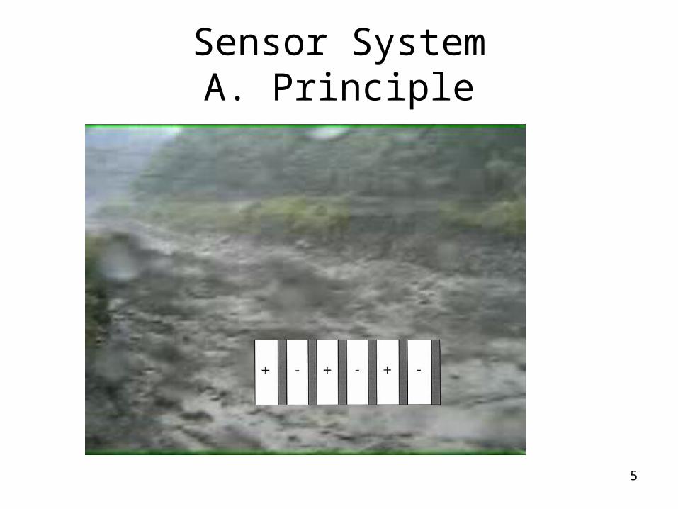
Sensor SystemA. Principle

Ω=V/HΩ: image velocityV: surface velocity of flowH: distance between the flow surface and sensor

5

Sensor SystemA. Principle

6

Sensor SystemA. Principle

• Time-varying output signal

• Equation(1) can be simplified as follows[1]:

– I(u,v) is the Fourier transform of i(x,y)– au /20

[1]. M. S. Uddin, H. Inaba, Y. Itakura, and M. Kasahara, “Estimation of the surface velocity of debris flow with computer-based spatial filtering,” Appl. Opt. 37, 6234-6239 (1998).

7

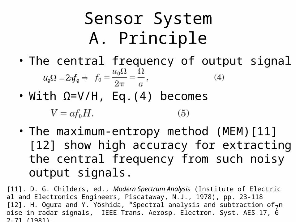
Sensor SystemA. Principle

• The central frequency of output signal

• With Ω=V/H, Eq.(4) becomes

• The maximum-entropy method (MEM)[11][12] show high accuracy for extracting the central frequency from such noisy output signals.

[11]. D. G. Childers, ed., Modern Spectrum Analysis (Institute of Electrical and Electronics Engineers, Piscataway, N.J., 1978), pp. 23-118[12]. H. Ogura and Y. Yoshida, “Spectral analysis and subtraction of noise in radar signals,” IEEE Trans. Aerosp. Electron. Syst. AES-17, 62-71 (1981).

00 2 fu

8

Sensor SystemA. Principle

9

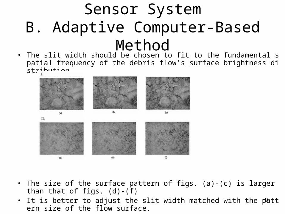
Sensor SystemB. Adaptive Computer-Based Method• The slit width should be chosen to fit to the fundamental spatial frequenc

y of the debris flow’s surface brightness distribution.

• The size of the surface pattern of figs. (a)-(c) is larger than that of figs. (d)-(f)

• It is better to adjust the slit width matched with the pattern size of the flow surface.

10

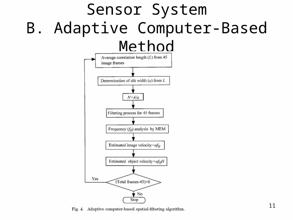
Sensor SystemB. Adaptive Computer-Based Method

• We try to calculate spatial correlation length...

• From the plot of R(k), the value of k when the normalized R(k) falls to (1/e)(=0.367), is treated as the correlation length.

K=5

11

Sensor SystemB. Adaptive Computer-Based Method

12

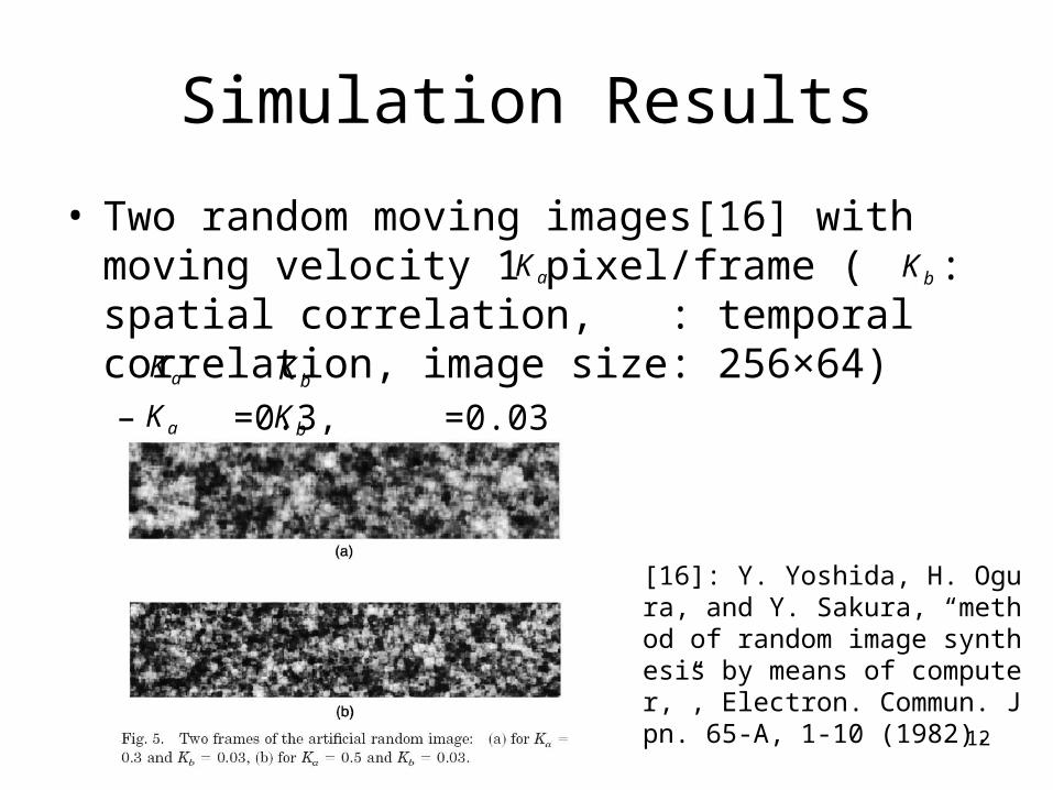
Simulation Results

• Two random moving images[16] with moving velocity 1 pixel/frame ( : spatial correlation, : temporal correlation, image size: 256×64)– =0.3, =0.03– =0.5, =0.03aK bK

aK

aK

bK

bK

[16]: Y. Yoshida, H. Ogura, and Y. Sakura, “method of random image synthesis by means of computer,”, Electron. Commun. Jpn. 65-A, 1-10 (1982).

13

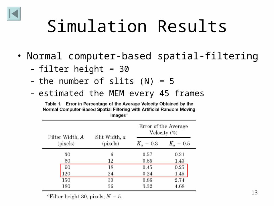
Simulation Results

• Normal computer-based spatial-filtering– filter height = 30

– the number of slits (N) = 5

– estimated the MEM every 45 frames

14

Simulation Results

• Adaptive computer-based spatial-filtering (correlation rectangle:120×30)– If L<6 → a=6– If L>A/ → a=A/ ( =5)minNminNminN

15

Simulation Results

16

Velocity Estimation Results of Debris Flow

• The video images of a debris flow that occurred on 14 July 1993 at the Mt. Yakedake Volcano, Japan

• Correlation rectangle: 120×50• Filter size: 450×128

17

Velocity Estimation Results of Debris Flow

• Rapid temporal fluctuations in the surface– The moving average method[17] with a smoothing

window length of 5

M

Mks tykxg

Mtyxg ),,(

12

1),,(

[17] A. V. Oppenheim and R. W. Schafer, Discrete-time Signal Processing(Prentice-Hall, New Delhi, India, 1994), pp. 17-18

18

Conclusions

• We compare adaptive computer-based spatial-filtering, normal computer-based spatial-filtering, and hardware-based spatial-filtering in this paper.

• The adaptive method can be the most accurate because of its ability to adjust the filter parameters for tuning the spatial filter to the stochastic characteristics of the flow.

19

Thank you!