1

14.02 Recitation

By

Samer HajYehia

2

The Short RunI. Course Introduction

II. Mathematical Background

III. Real vs. Nominal & Growth Rate

IV. National Account

V. Government Budget

VI. Basic Macroeconomic Model– Kenyes Model

VII. The Investment Saving Equilibrium

VIII.The IS Curve

IX. LM Curve

X. IS-LM Model

3

I. Course Introduction

a) Course Strategy

b) Course Outlines

c) Macro vs. Micro

d) Why Are You Taking Macroeconomics?

4

I(a) Course Strategy

Define the important concepts, magnitudes and questions in the real world.

Learn alternative theories suggesting answers and explaining behavior.

Evaluate data to test and then choose among theories.

Put you in position to have a serious opinion on important topics.

5

I(b) Macro vs. Micro Microeconomics examines the economic behavior of individual households

and firms-- their responses to prices, income, tastes, opportunities and other fundamental variables.

Macroeconomics examines the sum of microeconomic actions, their dynamics & interactions.

Therefore Macro must be fully compatible with Micro in its explanations of behavior: to trust any Macro answer, you must be sure of each of its Micro roots. Usually, this requires common sense and introspection.

The power and elegance of Macro is its ability to confront important questions, resolve paradoxes, explain past and predict future dynamics.

Why is there so much controversy about macro theory and policy and so little about micro?

Macro hits us in the pocketbook through its policy prescriptions so we may want certain answers to be true even if not.

Macro gets intimately involved in politically sensitive issues, and only religious arguments are more emotional than political debates.

The media cares about these issues and wants to find/exaggerate controversy to sell itself.

6

I(c) Why Are You Taking Macroeconomics? • Possible reasons:  It’s required for economics majors.  You’ve heard it’s as good a way as any to meet distribution requirements in

the social sciences since this will at least involve mathematics.  Economist jokes are better than lawyer or computer nerd jokes.  You want to call in to talk- show radio hosts and sound important.

• Better reasons: You know that, today or tomorrow, you will really need the macroeconomic

analysis skills as:

   An investor:

   a politician

   a manager or employee

   an intellectually curious person

7

       Your interest might be as following:

   An investor:   Where are interest rates headed?   Which sectors of the economy will do best and worst during the next

quarter, year, and decade?   What will be the distinguishing differences across countries.

   A politician   What determines interest rates and what are appropriate monetary

targets?   What are the appropriate taxes to raise?   How will the level and composition of the budget affect family incomes?   How will international trade impact jobs, inflation and credit?   What is the cost of low inflation or low unemployment?

8

   a manager or employee

 What growth will my current markets provide if I maintain my share?

 Can I raise my prices as rapidly as my costs?

 What opportunities are emerging in the developing nations?

    a manager or employee

 Why do cycles exist/ persist in all economies?

 Are macro relationships stable?

 Can nonlinear mathematics and chaos physics help to understand economics?

 How can growth and environmental concerns be reconciled?

9

I(d) Course Outlines

Output- level, growth, trend, fluctuations (recessions and expansions). Great Depression Stagflation in the 1970s Current long expansion and low unemployment High stock markets and bubbles From budget deficit to budget surplus Who is Greenspan? Why is he worry? Why we care? Asian 1980’s miracle and 1990’s crisis and the political consequences Russia and Latin America financial crises European Community (EC) Foreign trade Financial markets Globalization

10

II. Mathematical background

a) Linearity

b) Curve shifting

c) Adjacent or Stacked Graphs

d) Changes and Logarithm

e) Elasticity

11

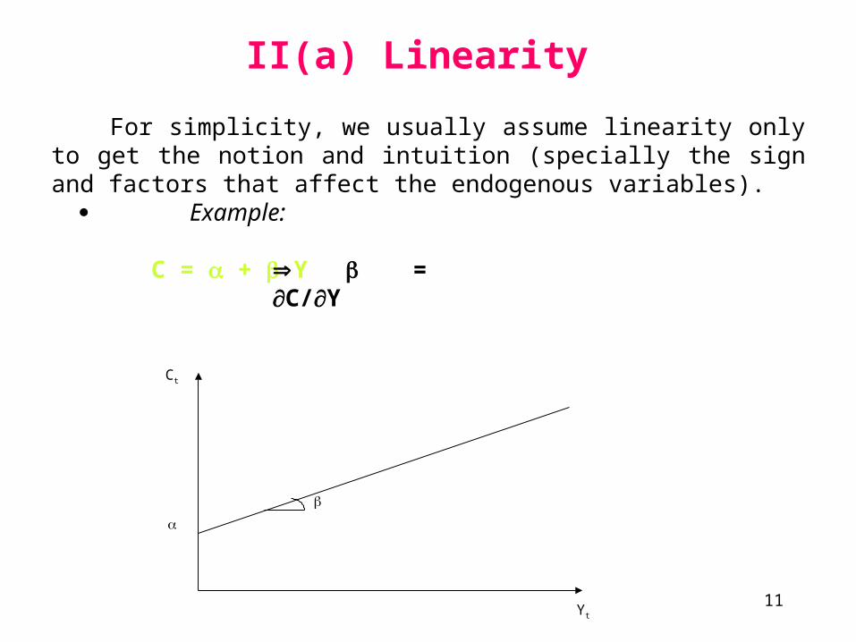
II(a) Linearity

Yt

Ct

    For simplicity, we usually assume linearity only to get the notion and intuition (specially the sign and factors that affect the endogenous variables). 

       Example:  C = + Y = C/Y

12

II(b) Curves, which way do they shift?

13

II(c) Adjacent or Stacked Graphs

14

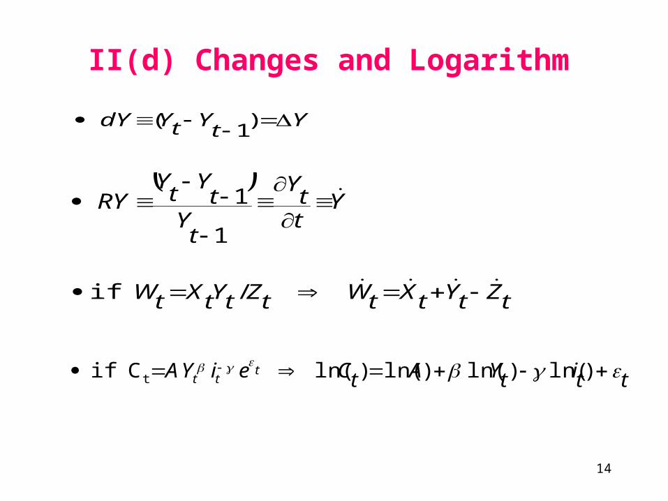
II(d) Changes and Logarithm

Y

tt

Y

tY

tY

tY

RY

1

1

tZtYtXtWtZtYtXtW / if

Yt

YtYdY )1

(

ttitYAtCeiYA ttt )ln( )ln( )ln( )ln( C if t

15

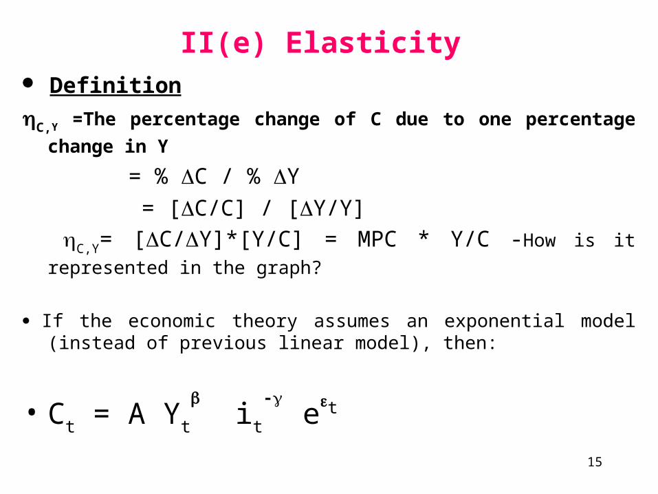
II(e) Elasticity Definition

C,Y =The percentage change of C due to one percentage change in Y

= % C / % Y

= [C/C] / [Y/Y]

C,Y= [C/Y]*[Y/C] = MPC * Y/C -How is it represented in the graph?

 If the economic theory assumes an exponential model (instead of previous linear model), then:

• Ct = A Yt

it

- et

16

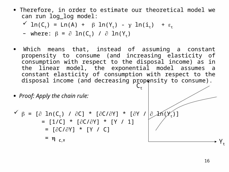
Therefore, in order to estimate our theoretical model we can run log_log model: ln(Ct) = Ln(A) + ln(Yt) - ln(it) + t

– where: = ln(Ct) / ln(Yt)

Which means that, instead of assuming a constant propensity to consume (and increasing elasticity of consumption with respect to the disposal income) as in the linear model, the exponential model assumes a constant elasticity of consumption with respect to the disposal income (and decreasing propensity to consume).

Proof: Apply the chain rule:

= [ ln(Ct) / C] * [C/Y] * [Y / ln(Yt)]

= [1/C] * [C/Y] * [Y / 1] = [C/Y] * [Y / C]

= C,Y

Ct

Yt

17

III. Real vs. Nominal & Growth Rate

a) An Exercise

b) Nominal vs. Real

18

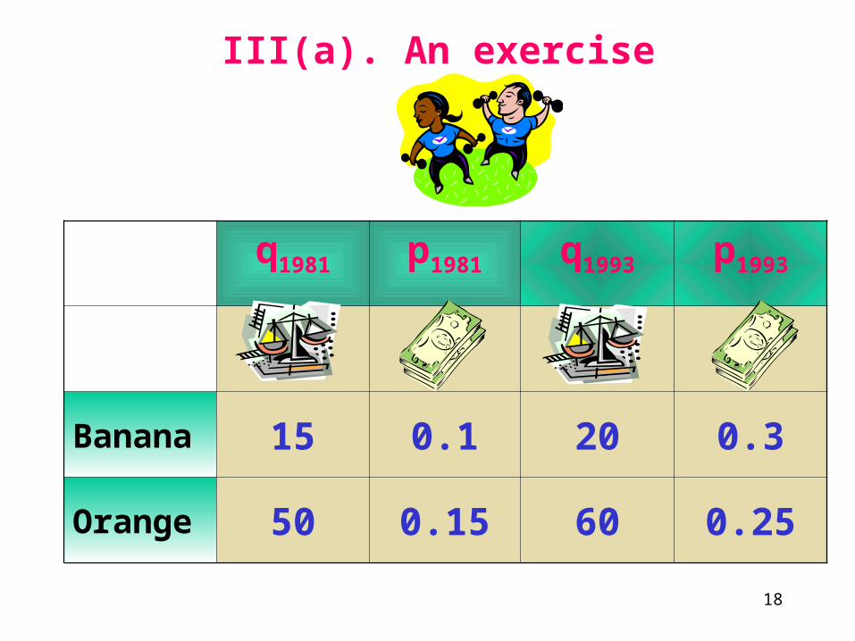
q1981 p1981 q1993 p1993

Banana 15 0.1 20 0.3

Orange 50 0.15 60 0.25

III(a). An exercise

19

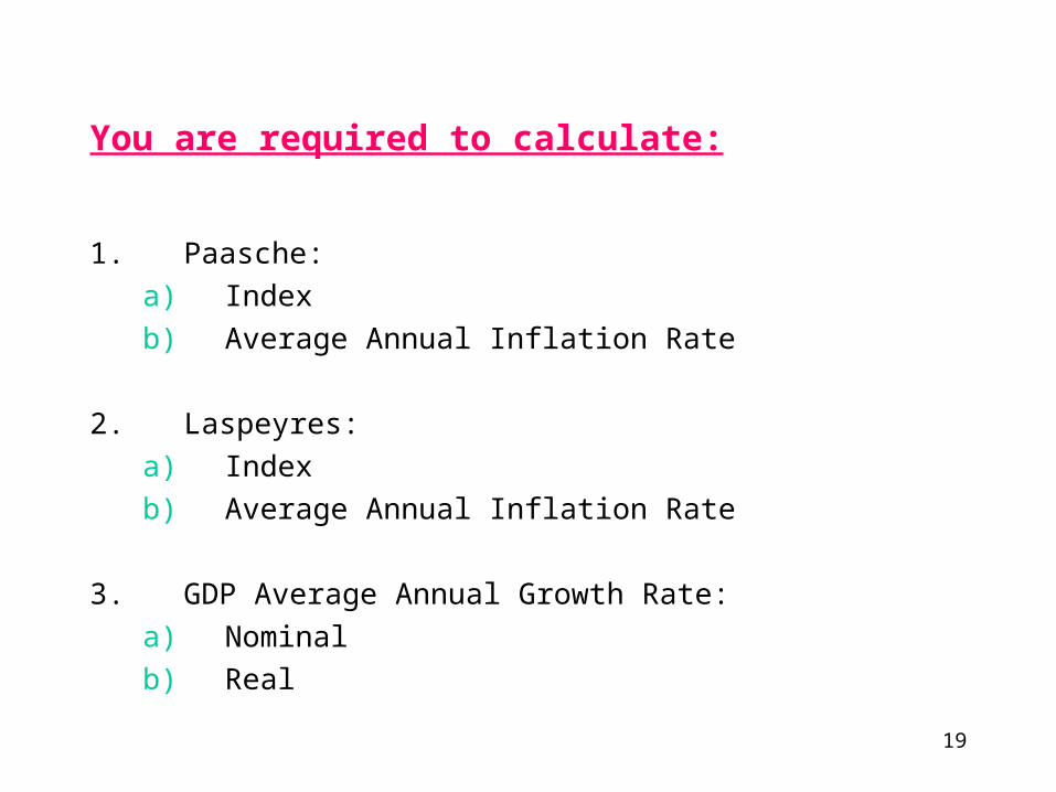
You are required to calculate:

1. Paasche:

a) Index

b) Average Annual Inflation Rate

2. Laspeyres:

a) Index

b) Average Annual Inflation Rate

3. GDP Average Annual Growth Rate:

a) Nominal

b) Real

20

You have 5 minutes

Can we start???

21

22

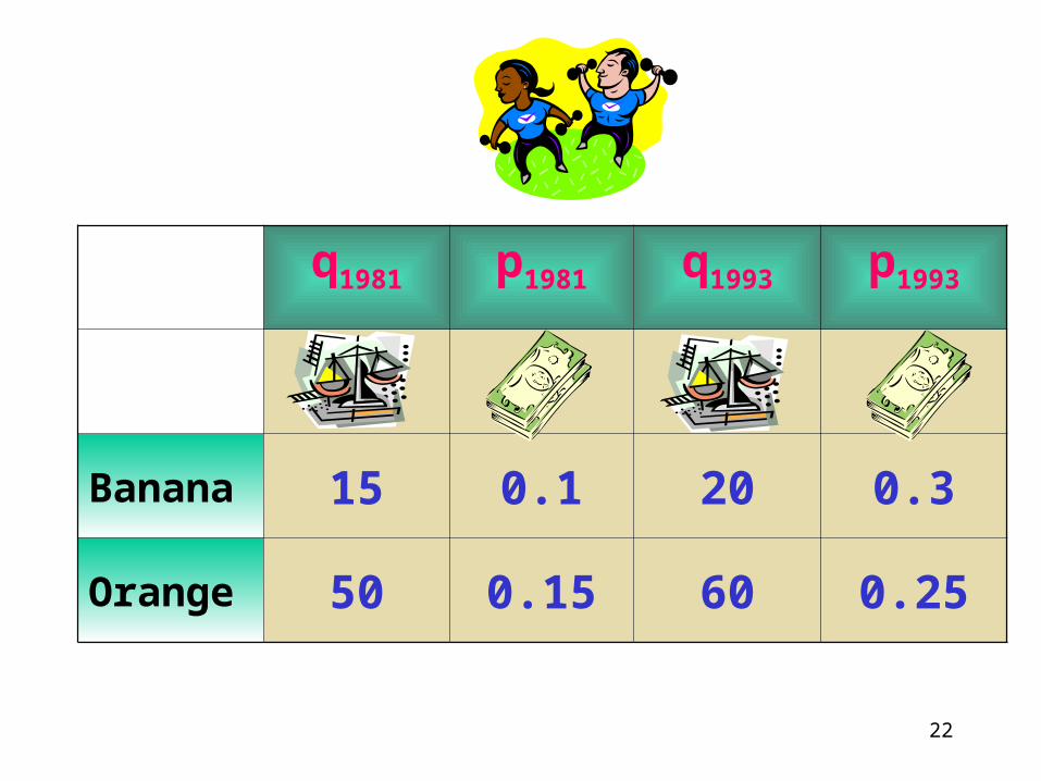
q1981 p1981 q1993 p1993

Banana 15 0.1 20 0.3

Orange 50 0.15 60 0.25

23

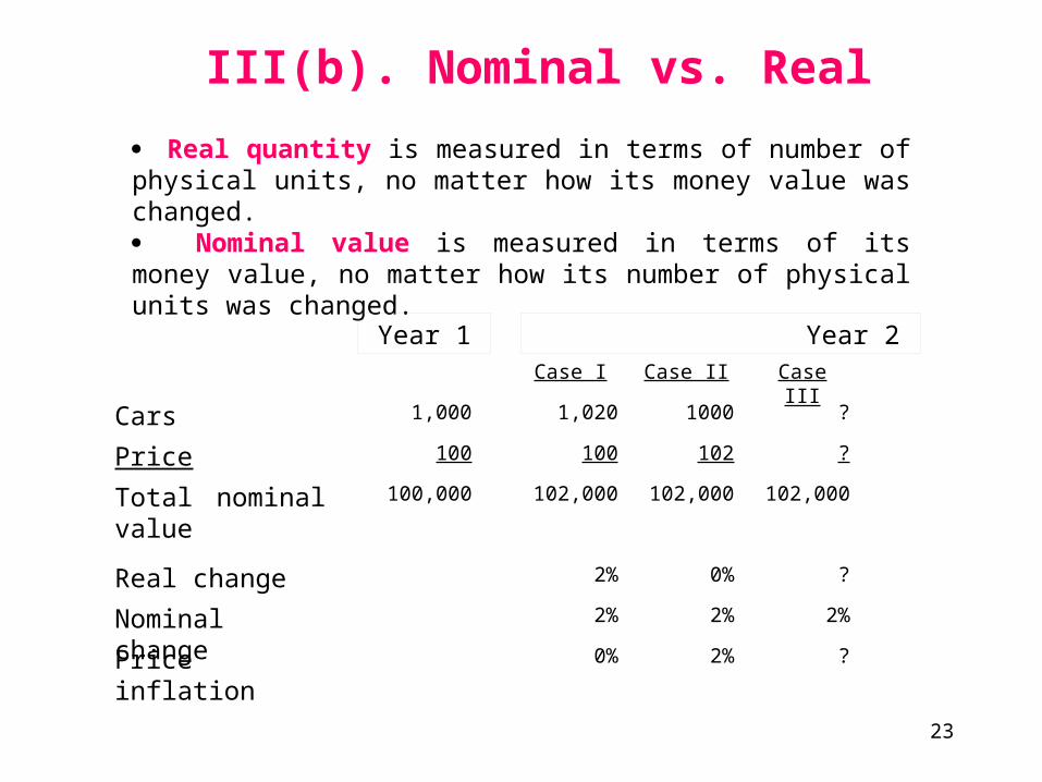
III(b). Nominal vs. Real

    Real quantity is measured in terms of number of physical units, no matter how its money value was changed.       Nominal value is measured in terms of its money value, no matter how its number of physical units was changed.

     

        Case I Case II Case III

Cars   1,000   1,020 1000 ?

Price   100   100 102 ?

Total nominal value   100,000   102,000 102,000 102,000

             

Real change       2% 0% ?

Nominal change       2% 2% 2%

Price inflation       0% 2% ?

Year 1 Year 2

24

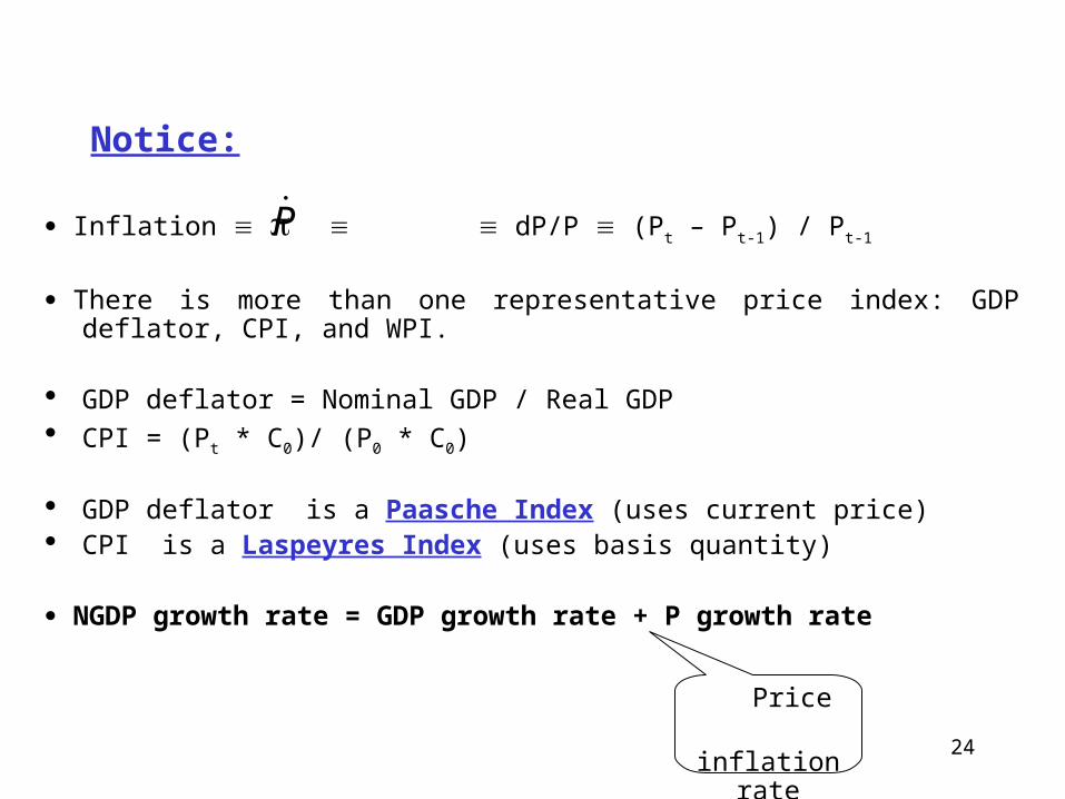
Notice:

 Inflation dP/P (Pt – Pt-1) / Pt-1

 There is more than one representative price index: GDP deflator, CPI, and WPI.

GDP deflator = Nominal GDP / Real GDP CPI = (Pt * C0)/ (P0 * C0)

GDP deflator is a Paasche Index (uses current price) CPI is a Laspeyres Index (uses basis quantity)

 NGDP growth rate = GDP growth rate + P growth rate

P

Price inflation

rate

25

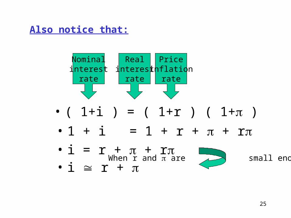
Also notice that:

• ( 1+i ) = ( 1+r ) ( 1+ )

Nominalinterest

rate

Realinterest

rate

Priceinflation

rate

When r and are small enough

• 1 + i = 1 + r + + r• i = r + + r• i r +

26

III(c). Another Real versus Nominal Exercise

27

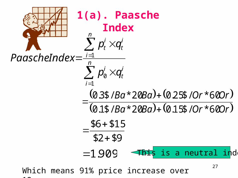
1(a). Paasche Index

n

i

it

i

n

i

it

it

qp

qpIndexPaasche

10

1

OrOrBaBa

OrOrBaBa

60*/$15.020*/$1.0

60*/$25.020*/$3.0

9$2$

15$6$

909.1 Which means 91% price increase over 12 years.

This is a neutral index

28

1(b). Paasche Average Annual Inflation Rate

= (1.909)1/12 –1 5.54%

29

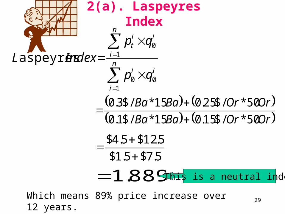
2(a). Laspeyres Index

n

i

ii

n

i

iit

qp

qpIndexL

100

10

aspeyres

OrOrBaBa

OrOrBaBa

50*/$15.015*/$1.0

50*/$25.015*/$3.0

5.7$5.1$

5.12$5.4$

889.1 Which means 89% price increase over 12 years.

This is a neutral index

30

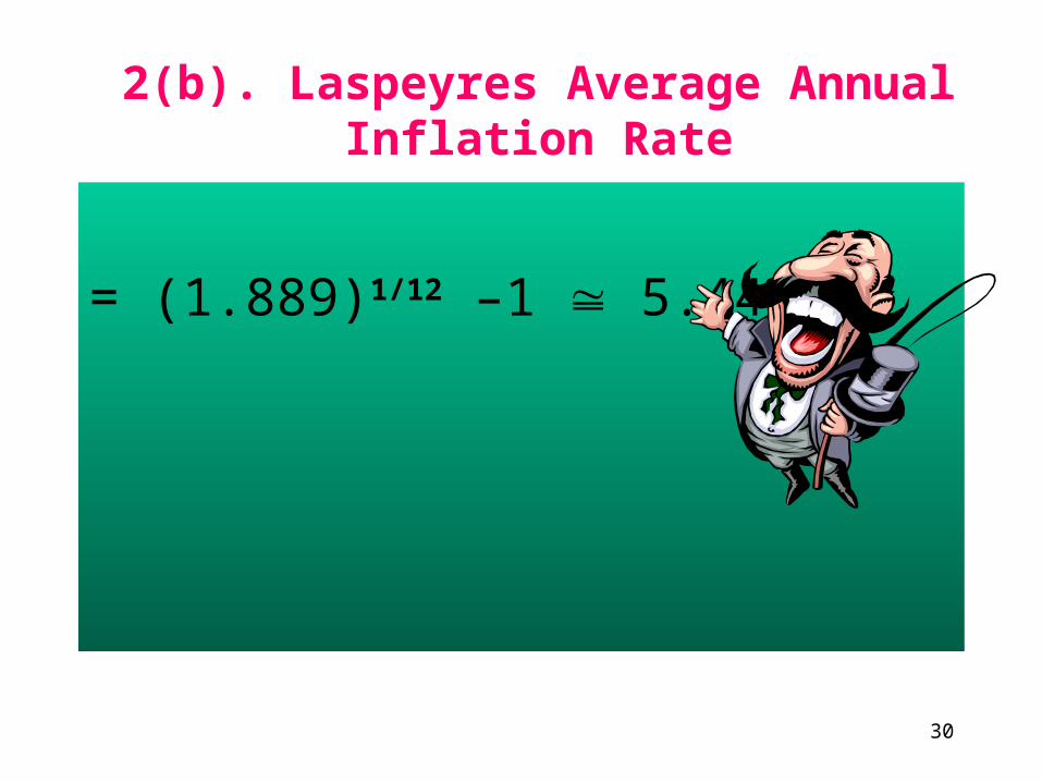
2(b). Laspeyres Average Annual Inflation Rate

= (1.889)1/12 –1 5.44%

31

1

12/1

100

1

n

i

ii

n

i

it

it

qp

qpY

1

50*/$15.015*/$1.0

60*/$25.020*/$3.0

12/1

OrOrBaBa

OrOrBaBa

15.7$5.1$

15$6$

12/1

%32.7

3(a). Nominal GDP Annual Growth Rate

32

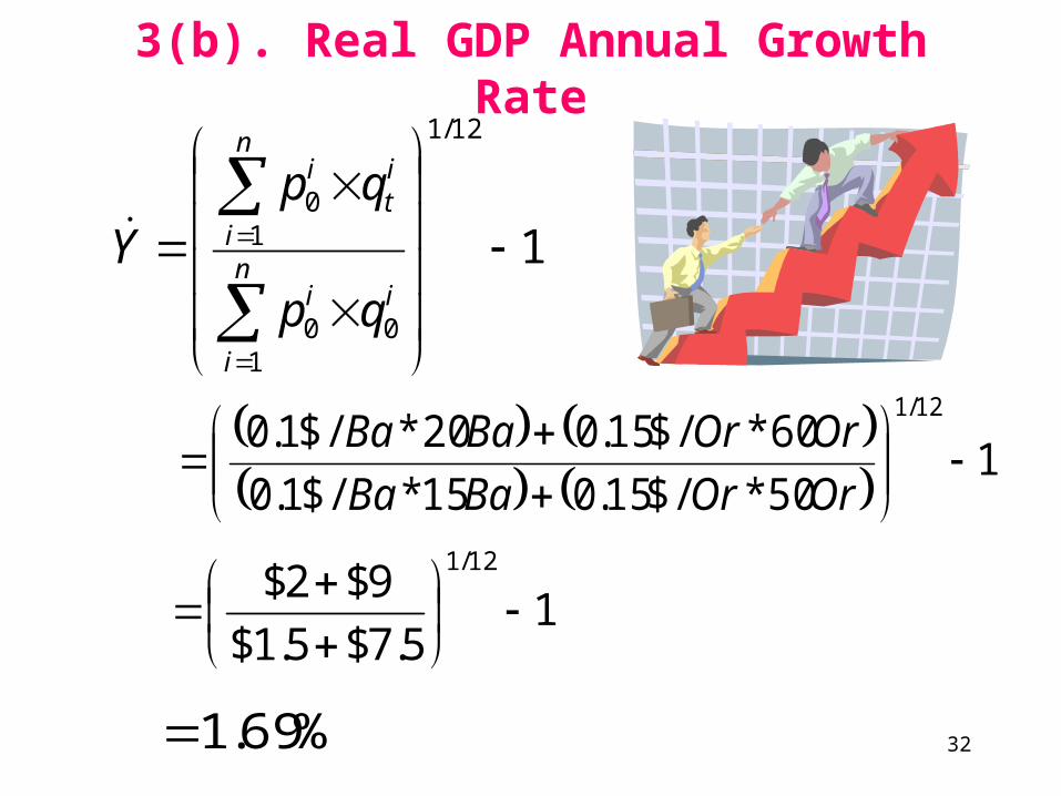
3(b). Real GDP Annual Growth Rate

1

12/1

100

10

n

i

ii

n

i

it

i

qp

qpY

1

50*/$15.015*/$1.0

60*/$15.020*/$1.0

12/1

OrOrBaBa

OrOrBaBa

15.7$5.1$

9$2$

12/1

%69.1

33

IV. The National Accounting

a) Key players

b) Counting the GDP

c) Counting the GDP- an example

d) Other definitions

e) A Summary: The Relationships among the basic spending and income categories

34

IV(a) Key players        The key actors in the macro economy:

Firms: (domestically) producing (Y) and investing (I) entities.Y = GDP

Households: consuming (C) and saving (S) entities. YD = Y – T, YD = C + Sp , Sp = YD – C

Government Agencies: raise net taxes (T=T0 + t*Y -Tr), spend on public goods (G) and pay interest on their debt. Sg = T – G, BD = G – T

Central Bank: controls the interest rates (i) through the money supply (M).

Foreign counterparts: we export products to them (EX) and import products from them (IM) and exchange financial assets with them.NX = EX - IM

Y = C + G + I + EX – IM .

35

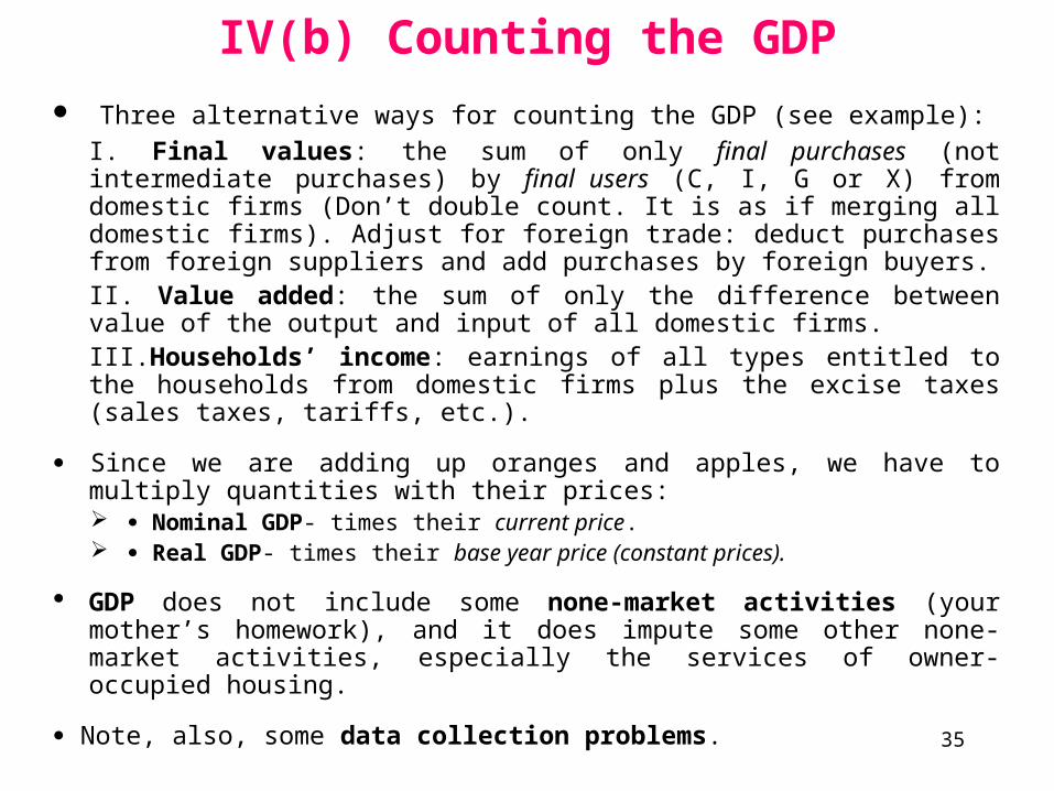
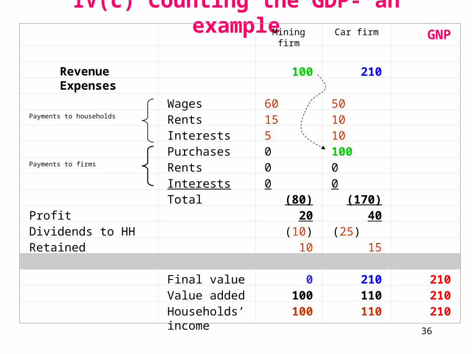
IV(b) Counting the GDP

Three alternative ways for counting the GDP (see example):

I. Final values: the sum of only final purchases (not intermediate purchases) by final users (C, I, G or X) from domestic firms (Don’t double count. It is as if merging all domestic firms). Adjust for foreign trade: deduct purchases from foreign suppliers and add purchases by foreign buyers.II. Value added: the sum of only the difference between value of the output and input of all domestic firms.III.Households’ income: earnings of all types entitled to the households from domestic firms plus the excise taxes (sales taxes, tariffs, etc.).

Since we are adding up oranges and apples, we have to multiply quantities with their prices: Nominal GDP- times their current price. Real GDP- times their base year price (constant prices).

GDP does not include some none-market activities (your mother’s homework), and it does impute some other none-market activities, especially the services of owner-occupied housing.

Note, also, some data collection problems.

36

IV(c) Counting the GDP- an example

RevenueExpenses

    Mining firm Car firm GNP

           100 210         

  Wages 60 50  Payments to households Rents 15 10    Interests 5 10  

Purchases 0 100  Payments to firms Rents 0 0    Interests 0 0    Total (80) (170)  Profit   20 40  Dividends to HH   (10) (25)  Retained earnings   10 15             Final value 0 210 210  Value added 100 110 210  Households’

income100 110 210

37

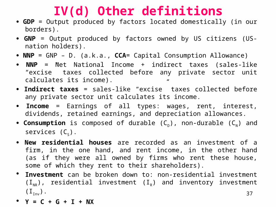
IV(d) Other definitions GDP = Output produced by factors located domestically (in our borders).

GNP = Output produced by factors owned by US citizens (US-nation holders).

NNP = GNP – D. (a.k.a., CCA= Capital Consumption Allowance)

NNP = Net National Income + indirect taxes (sales-like “excise” taxes collected before any private sector unit calculates its income).

Indirect taxes = sales-like “excise” taxes collected before any private sector unit calculates its income.

Income = Earnings of all types: wages, rent, interest, dividends, retained earnings, and depreciation allowances.

Consumption is composed of durable (CD), non-durable (CN) and services

(CS).

New residential houses are recorded as an investment of a firm, in the one hand, and rent income, in the other hand (as if they were all owned by firms who rent these house, some of which they rent to their shareholders).

Investment can be broken down to: non-residential investment (INR),

residential investment (IR) and inventory investment (IInv).

Y = C + G + I + NX

38

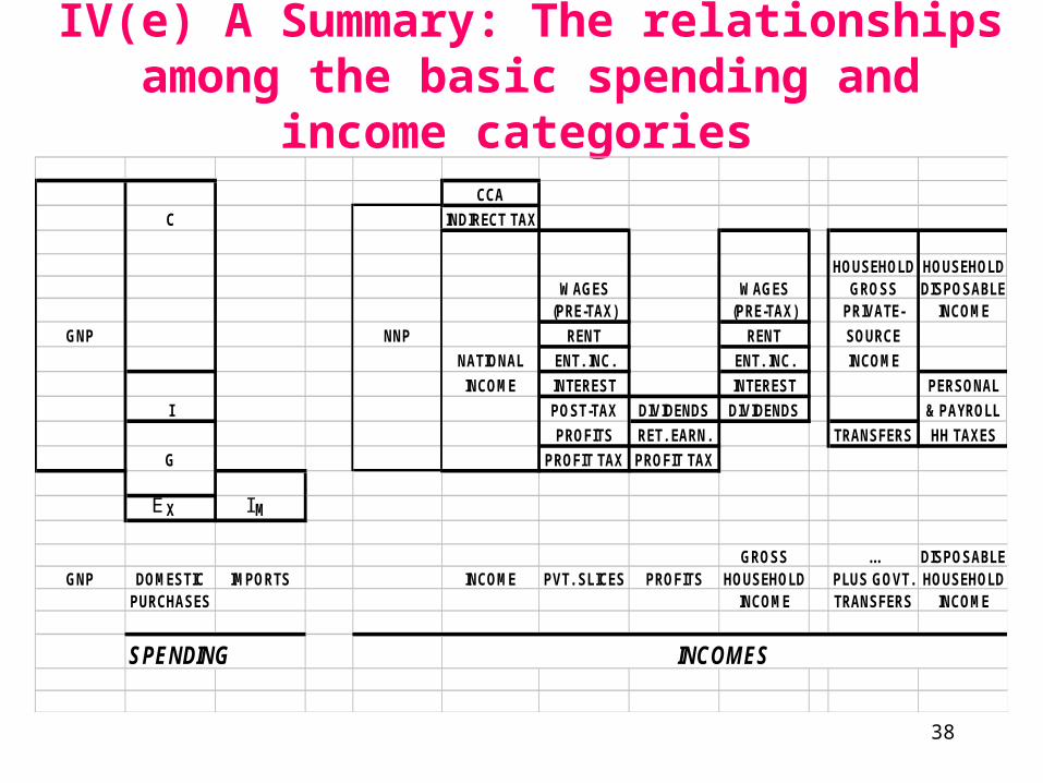
IV(e) A Summary: The relationships among the basic spending and income categories

CCA

C INDIRECT TAX

HOUSEHOLD HOUSEHOLD WAGES WAGES GROSS DISPOSABLE

(PRE-TAX) (PRE-TAX) PRIVATE- INCOME

GNP NNP RENT RENT SOURCE

NATIONAL ENT. INC. ENT. INC. INCOME

INCOME INTEREST INTEREST PERSONAL

I POST-TAX DIVIDENDS DIVIDENDS & PAYROLL

PROFITS RET. EARN. TRANSFERS HH TAXES

G PROFIT TAX PROFIT TAX

X M

GROSS ... DISPOSABLEGNP DOMESTIC IMPORTS INCOME PVT. SLICES PROFITS HOUSEHOLD PLUS GOVT. HOUSEHOLD

PURCHASES INCOME TRANSFERS INCOME

SPENDING INCOMES

IE

39

(V) The Government Budget

a) Definitions

b) The Federal Budget

c) State & Local Budgets

40

V(a) Definitions

 G: is all the purchases of goods and services made by the government

 It does NOT including government transfers or interest rate payments (otherwise, you will get double counting).

 Government outlays include them all: purchases of goods and services, transfers and or interest rate payments made by the government.

 Net Taxes are total taxes after deducting government transfers.

Government includes the Federal, State and local government agencies.

Note their decomposition of budget.

41

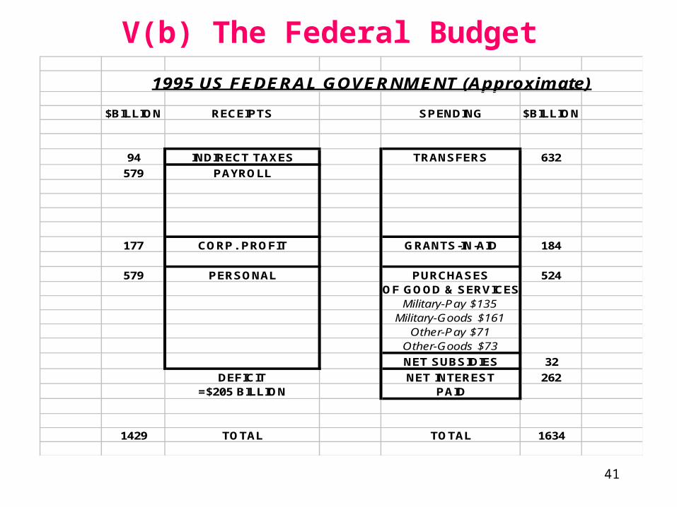
V(b) The Federal Budget

1995 US FEDERAL GOVERNMENT (Approximate)

$BILLION RECEIPTS SPENDING $BILLION

94 INDIRECT TAXES TRANSFERS 632

579 PAYROLL

177 CORP. PROFIT GRANTS-IN-AID 184

579 PERSONAL PURCHASES 524OF GOOD & SERVICES

Military-Pay $135Military-Goods $161

Other-Pay $71 Other-Goods $73

NET SUBSIDIES 32

DEFICIT NET INTEREST 262=$205 BILLION PAID

1429 TOTAL TOTAL 1634

42

VI. Basic Macroeconomic Model– Kenyes Modela) Key players

b) Behavioral (simultaneous) equations for the endogenous variables

c) Exogenous variables

d) Identity (definition) equations

e) Equilibrium condition in the goods market

f) A graphical presentation

g) A fiscal expansion: Gh) A monetary contraction: ii) Reduced form of the endogenous variables

43

Money Market

(M,i)

Labor Market

(L,W)Goods Market

(Y,P) IS curve

LM curve Currency Market

(€,)

AD-ASCurves

AS curve

AD curve

44

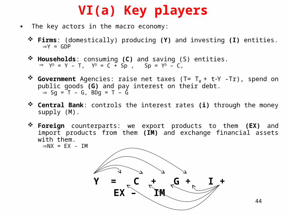
VI(a) Key players        The key actors in the macro economy:

Firms: (domestically) producing (Y) and investing (I) entities.Y = GDP

Households: consuming (C) and saving (S) entities. YD = Y – T, YD = C + Sp , Sp = YD – C,

Government Agencies: raise net taxes (T= T0 + t*Y -Tr), spend on public goods (G) and pay interest on their debt. Sg = T – G, BDg = T – G

Central Bank: controls the interest rates (i) through the money supply (M).

Foreign counterparts: we export products to them (EX) and import products from them (IM) and exchange financial assets with them.NX = EX - IM

Y = C + G + I + EX – IM .

45

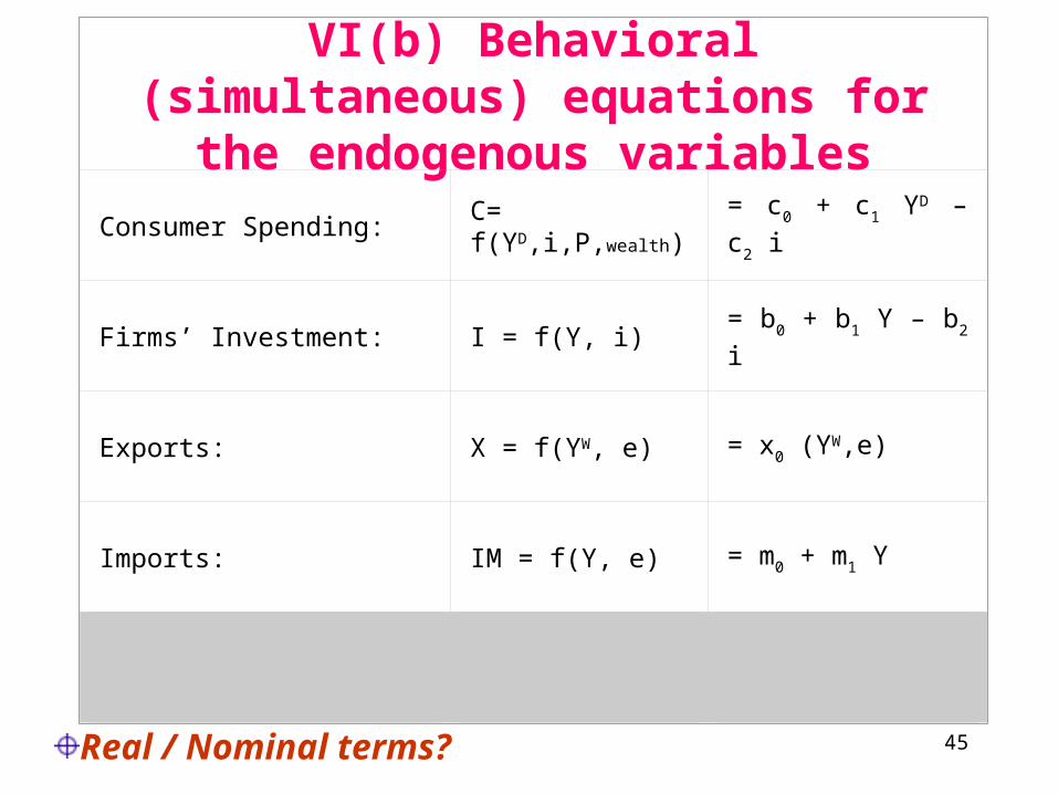
VI(b) Behavioral (simultaneous) equations for the endogenous variables

Consumer Spending: C= f(YD,i,P,wealth) = c0 + c1 YD – c2 i

Firms’ Investment: I = f(Y, i) = b0 + b1 Y – b2 i

Exports: X = f(YW, e) = x0 (YW,e)

Imports: IM = f(Y, e) = m0 + m1 Y

     

Real / Nominal terms?

46

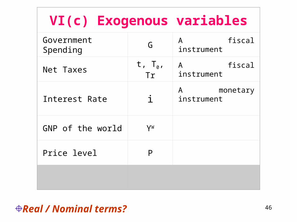
VI(c) Exogenous variables

Government Spending G A fiscal instrument

Net Taxes t, T0, Tr A fiscal instrument

Interest Rate i A monetary instrument

GNP of the world YW  

Price level P

     

Real / Nominal terms?

47

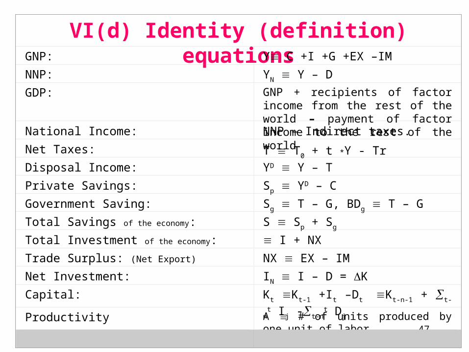
VI(d) Identity (definition) equationsGNP: Y C +I +G +EX –IM

NNP: YN Y – D

GDP: GNP + recipients of factor income from the rest of the world – payment of factor income to the rest of the world

National Income: NNP – Indirect taxes.

Net Taxes: T T0 + t *Y - Tr

Disposal Income: YD Y – T

Private Savings: Sp YD – C

Government Saving: Sg T – G, BDg T – G

Total Savings of the economy: S Sp + Sg

Total Investment of the economy: I + NX

Trade Surplus: (Net Export) NX EX – IM

Net Investment: IN I – D = K

Capital: Kt Kt-1 +It –Dt Kt-n-1 + t-nt Ij -t-n

t Dj

Productivity A # of units produced by one unit of labor

   

48

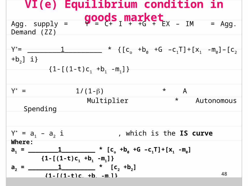
VI(e) Equilibrium condition in goods market

Agg. supply = Y = C+ I + +G + EX – IM = Agg. Demand (ZZ)

 

Y*= ________1_________ * {[co +b0 +G –c1T]+[x1 -m0]–[c2 +b2] i}

{1-[(1-t)c1 +b1 -m1]} 

Y* = 1/(1-) * A

Multiplier * Autonomous Spending

 

Y* = a1 – a2 i , which is the IS curveWhere:a1 = ________1_________ * [co +b0 +G –c1T]+[x1 -m0]

{1-[(1-t)c1 +b1 -m1]}

a2 = ________1_________ * [c2 +b2]

{1-[(1-t)c1 +b1 -m1]}   

49

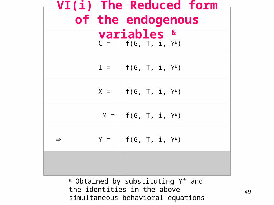
& Obtained by substituting Y* and the identities in the above simultaneous behavioral equations

VI(i) The Reduced form of the endogenous variables &

C = f(G, T, i, YW)

I = f(G, T, i, YW)

X = f(G, T, i, YW)

M = f(G, T, i, YW)

Y = f(G, T, i, YW)

   

50

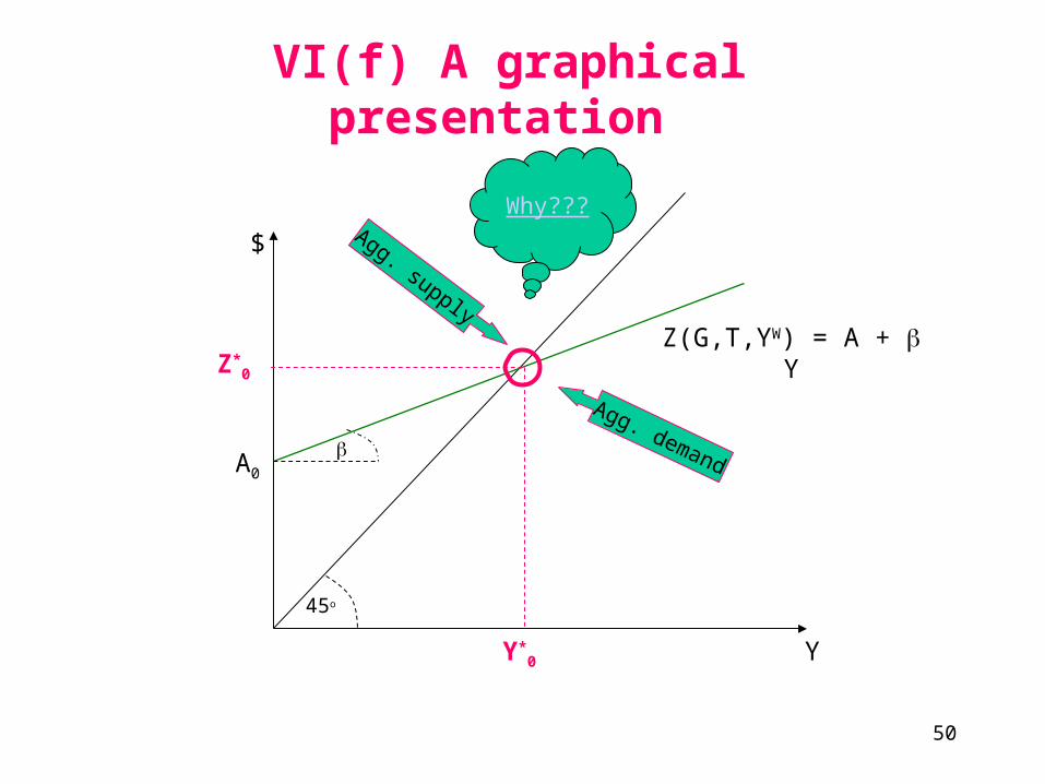
45o

A0

$

Z(G,T,YW) = A + Y

Y*0 Y

Agg. supply

Agg. demand

VI(f) A graphical presentation

Z*0

Why???

51

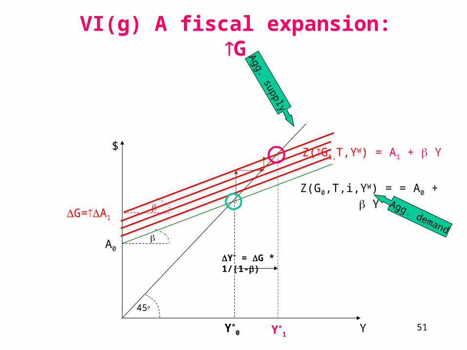
45o

A0

$

Z(G0,T,i,YW) = = A0 + Y

Y*0 Y

Z(G1,T,YW) = A1 + Y

Y*1

G=A1

Y* = G * 1/(1-)

A

gg. supply

Agg. demand

VI(g) A fiscal expansion: G

52

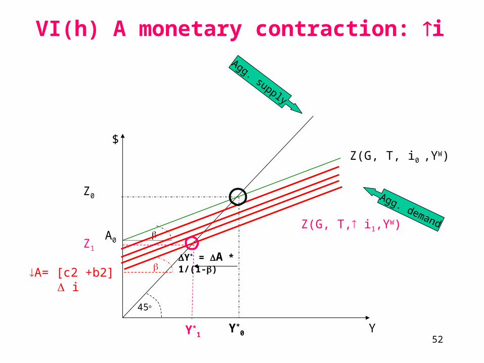
45o

A0

$Z(G, T, i0 ,YW)

Y*0 Y

Z(G, T, i1,YW)

Y*1

A= [c2 +b2] i Y* = A * 1/(1-)

Agg. supply

Agg. demand

VI(h) A monetary contraction: i

Z1

Z0

53

Exercise:

1. Suppose T = t Y.  Find equilibrium output for this case.  How does the multiplier here compare to the multiplier in the case where taxes do not depend on income?

2. If taxes depend on income, show the effect on equilibrium output of an increase in the tax rate.  First show the result graphically and then find the precise mathematical expression for the change in equilibrium output.

3. In the early 1980s, President Ronald Reagan proposed a cut in the tax rate.  He argued that such a cut would stimulate the economy so much that the government's budget deficit would be reduced. Is this possible in our model (again, supposing that taxes depend on income).  Prove your answer mathematically.

4. Suppose that imports depend on domestic income: IM = m0 + m1Y.  Also suppose that taxes depend on income.  Find the mathematical expression for equilibrium output.  How does the multiplier here compare to the multiplier in the case where imports does not depend on income?

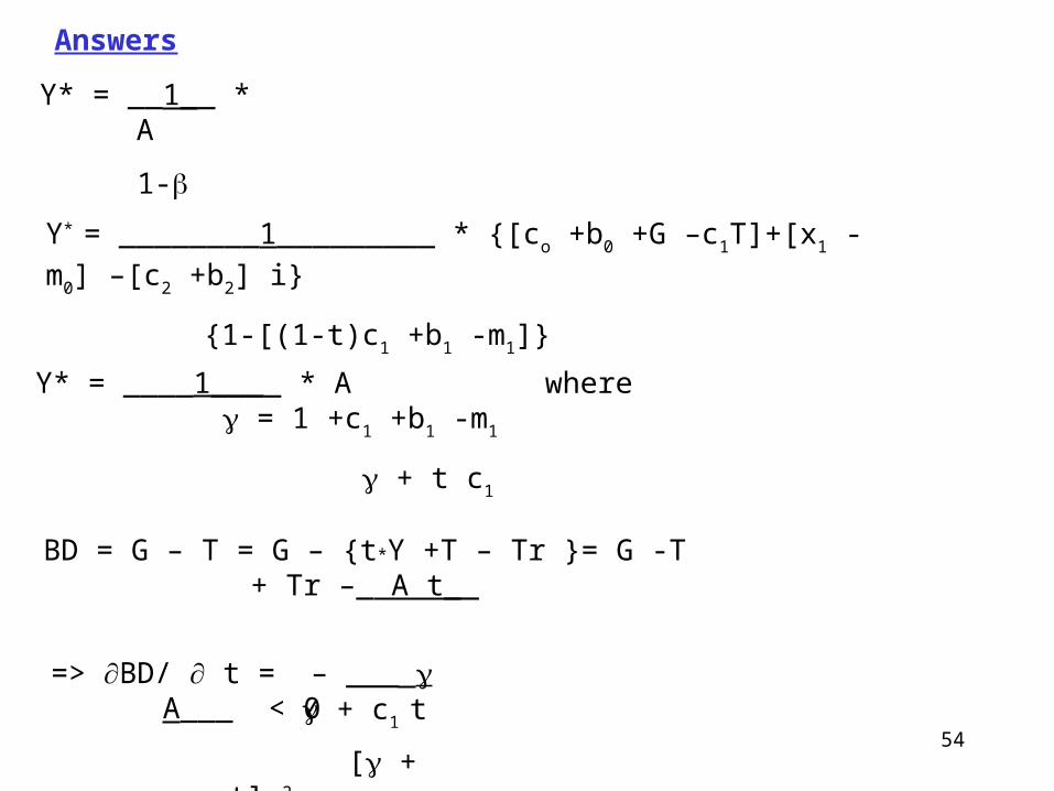
54

Y* = ________1_________ * {[co +b0 +G –c1T]+[x1 -m0] –[c2 +b2] i}

{1-[(1-t)c1 +b1 -m1]}

Answers

Y* = __1__ * A

1-

Y* = ____1____ * A where = 1 +c1 +b1 -m1

+ t c1

BD = G – T = G – {t*Y +T – Tr }= G -T + Tr –_ A t__

+ c1 t

=> BD/ t = – ___ A___ < 0

[ + c1 t] 2

55

Therefore::

Y* = __1__ * A

1-

Y* = { __1__ — __1__ }* A

1-1 1-0

Y*

Therefore:

t [(1-t)c1 +b1 -m1] (1-t)

1

1

(1-)

m [(1-t)c1 +b1 -m1] (1-)

Mu

ltipl i er1

1

1

56

45o

0A0

$

Z(G,t0,i,YW)

Y*0 Y

Agg. supply

Agg. demand

Z*0

1

Z*1

Y*1

Z(G, t1,i,YW)

Y* = A * [1/(1-1) - 1/(1-0)]

57

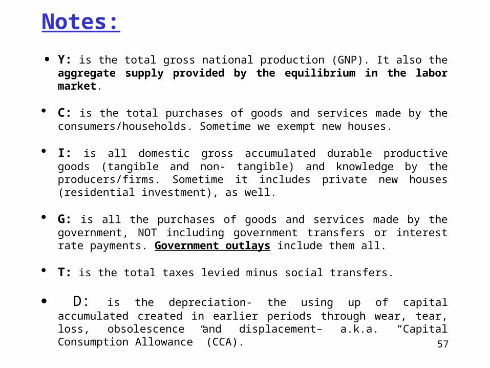
Notes:

• Y: is the total gross national production (GNP). It also the aggregate supply provided by the equilibrium in the labor market.

C: is the total purchases of goods and services made by the consumers/households. Sometime we exempt new houses.

I: is all domestic gross accumulated durable productive goods (tangible and non- tangible) and knowledge by the producers/firms. Sometime it includes private new houses (residential investment), as well.

G: is all the purchases of goods and services made by the government, NOT including government transfers or interest rate payments. Government outlays include them all.

T: is the total taxes levied minus social transfers.

  D: is the depreciation- the using up of capital accumulated created in earlier periods through wear, tear, loss, obsolescence and displacement– a.k.a. “Capital Consumption Allowance” (CCA).

58

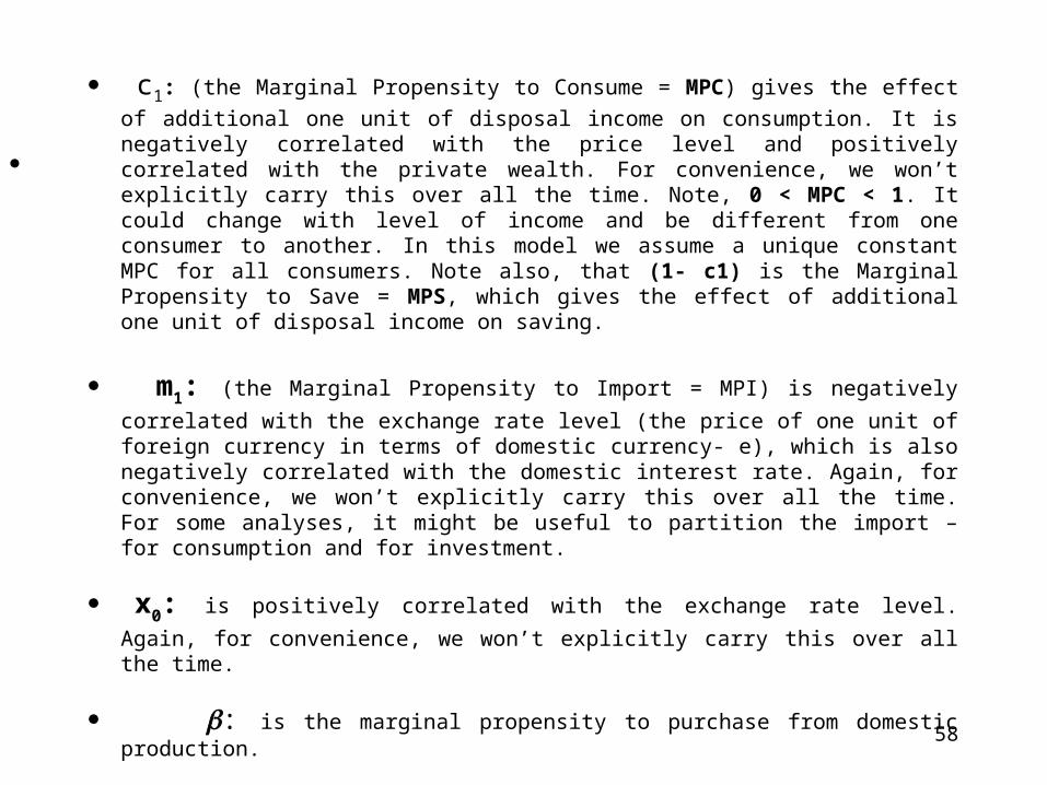
  c1: (the Marginal Propensity to Consume = MPC) gives the effect of

additional one unit of disposal income on consumption. It is negatively correlated with the price level and positively correlated with the private wealth. For convenience, we won’t explicitly carry this over all the time. Note, 0 < MPC < 1. It could change with level of income and be different from one consumer to another. In this model we assume a unique constant MPC for all consumers. Note also, that (1- c1) is the Marginal Propensity to Save = MPS, which gives the effect of additional one unit of disposal income on saving.

   m1: (the Marginal Propensity to Import = MPI) is negatively correlated with

the exchange rate level (the price of one unit of foreign currency in terms of domestic currency- e), which is also negatively correlated with the domestic interest rate. Again, for convenience, we won’t explicitly carry this over all the time. For some analyses, it might be useful to partition the import – for consumption and for investment.

  x0: is positively correlated with the exchange rate level. Again, for

convenience, we won’t explicitly carry this over all the time.

  : is the marginal propensity to purchase from domestic production.

      

59

VII. The Investment Saving Equilibrium

60

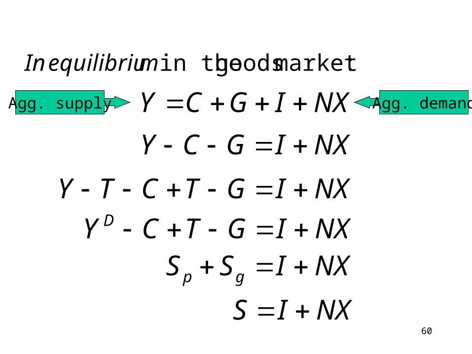
NXIGCY

mequilibriuIn

:market goods in the

NXIGCY

NXIGTCTY NXIGTCY D NXISS gp

NXIS

Agg. demandAgg. supply

61

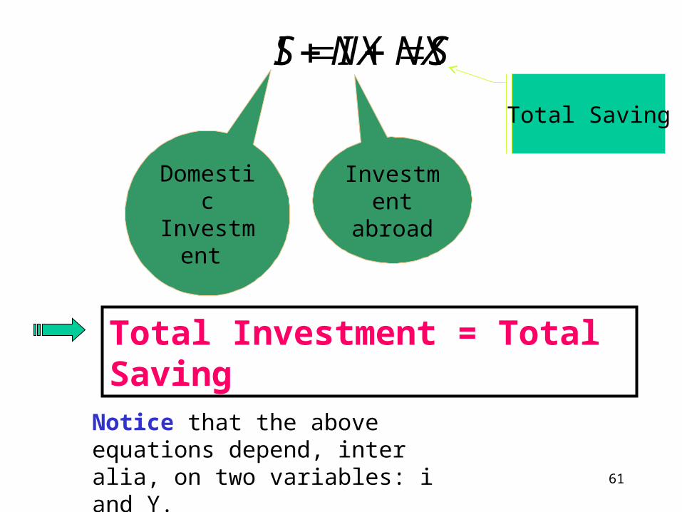
NXIS

Investment abroad

Domestic Investment

Total Saving

Total Investment = Total Saving

Notice that the above equations depend, inter alia, on two variables: i and Y.

SNXI

62

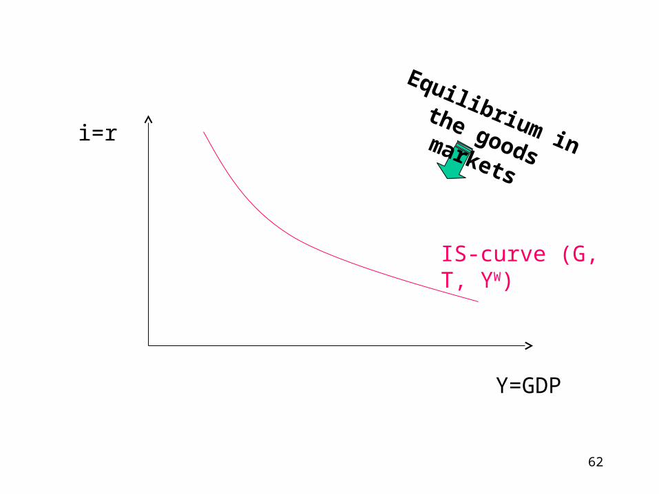
Y=GDP

i=r

IS-curve (G, T, YW)

Equilibrium in the

goods markets

63

VIII. IS Curve

a) Definition

b) The derivation of the IS curve

c) Shifts of the IS curve

64

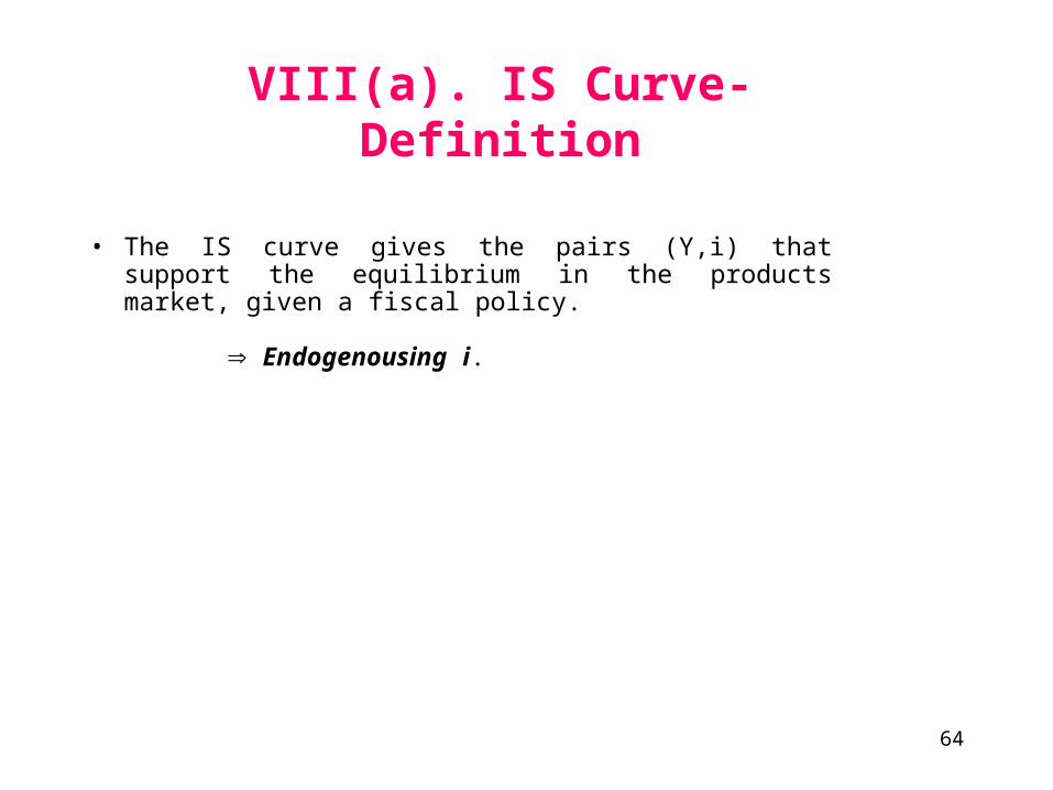
VIII(a). IS Curve- Definition

• The IS curve gives the pairs (Y,i) that support the equilibrium in the products market, given a fiscal policy.

Endogenousing i.

65

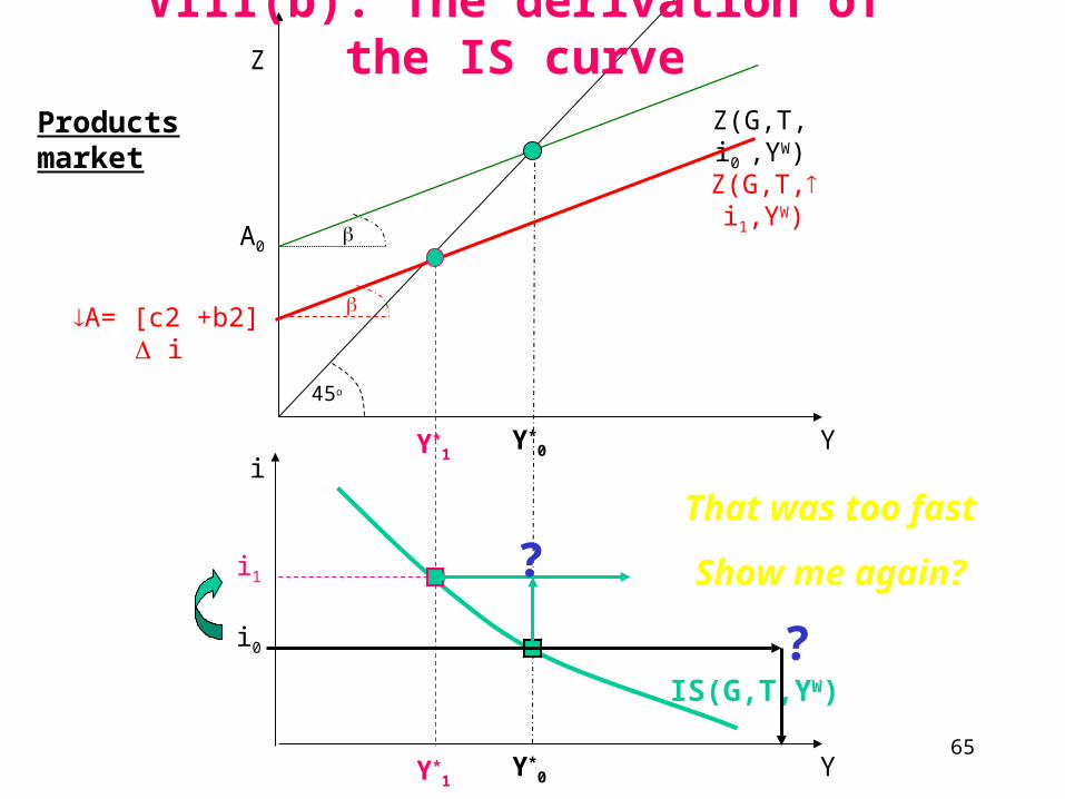
45o

A0

Z

Z(G,T, i0 ,YW)

Y*0 Y

Z(G,T, i1,YW)

Y*1

A= [c2 +b2] i

Products market

Y*0 Y

IS(G,T,YW)

Y*1

i1

i0

i

?

?

That was too fast

Show me again?

VIII(b). The derivation of the IS curve

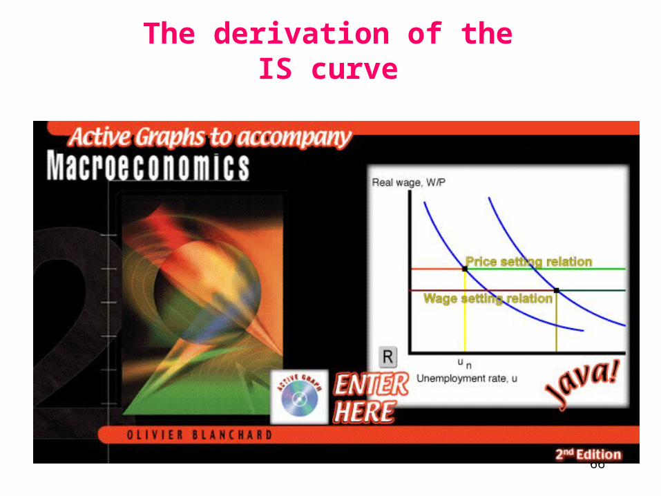
66

The derivation of the IS curve

67

VIII(c). Shifts of the IS curve

68

       The IS curve is flatter:

(a) the greater is the investment and consumption sensitivity to interest rates,

(b) the greater is the investment and consumption sensitivity to income.

Note:

69

IX. LM Curve

a) Definition

b) Money Demand Curve Shifts of the IS curve

c) The Quantity Theory

d) Money Supply Curve

e) The Equilibrium in the Money Market

f) The Interest rate determination in the money market

g) The derivation of the LM curve

h) Shifts of the LM curve

70

IX(a). LM Curve- Definition

• The LM curve gives the pairs (Y,i) that support the equilibrium in the financial market, given a monetary policy.

Endogenousing i.

71

IX(b). Money Demand Curve

1. Perfectly liquid- money (currency and checkable deposits): can be used for private spending (nominal product-transactions [barter is rare]), precautionary (possible unexpected future transactions), speculative motive (maximizing return on all assets in uncertain world), but it bears zero nominal yields.

2. Imperfectly liquid- bonds, stocks, options: not enough liquid for transaction, precautionary and speculative needs, but bear risky positive expected nominal yields.

•In holding your wealth accumulated from your savings, you need to decide how to allocate among different financial assets.

•Basically, two types of financial assets are available:

72

Notes:

• We focus on “money = currency and checkable depositsM1” rather than other assets (+savings +brokerage account)?

I. Traditionally, it was distinctive because it paid no tangible yield and was the only perfectly liquid asset.

II. The central bank was thought to have greater control over its supply.

• How do innovations in the financial market (introduction of credit card) affect demand for money?

• Be careful about defining the spending measure for private money holding: it’s not all of GDP. Why? Because remember that this is only the transaction demand component. (What about demand for investment?

73

• Therefore, it’s clear that the proportions (of perfect and imperfect liquid assets) that you choose depend on two variables:

I. Level of nominal transactions (+): this is highly correlated (proportional) with the private nominal income and spending.

II. Interest rate on bonds (-).

• Therefore, the behavioral demand function for nominal money- Md :

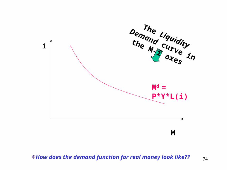
Md = P*Y*L(i)

• Or, equivalently:

(M/P) d = Y*L(i)

74

M

i

Md = P*Y*L(i)

The Liquidity Demand

curve in the M-i axes

How does the demand function for real money look like??

75

IX(c). The Quantity Theory • Define: velocity of money v P*Y/M. -This is called the quantity

equation.

• In words- the ratio of nominal income to money is higher, the number of transactions for a given quantity of money is higher, and it must be the case that money is changing hands faster. Put another way, the velocity is higher.

• Strict monetarism asserts, in the long run, Y (=Yn) and v are fixed in equilibrium. Therefore, P*Y = M * v, which means that the Fed can have a strict control over inflation via its control of the money (usually, was thought M1).

• Empirically, velocity is not fixed; rather it is sensitive to interest rates.

• See graph below.

• Still, the Fed can control the inflation via its grip on the money, , but (1) not as easy as it was thought, and (2) not by only controlling M1.

76

The Velocity of Money (M1) vs. the Treasury Bill Rate

5.0

5.5

6.0

6.5

7.0

7.5

8.0

8.5

9.0

9.5

10.0

0.00

2.00

4.00

6.00

8.00

10.00

12.00

14.00

16.00

Treasury Bill Rate Velocity (GDP / M1 )

77

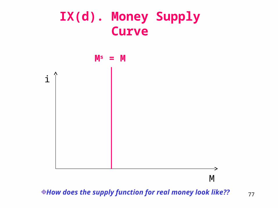
IX(d). Money Supply Curve

M

i

Ms = M

How does the supply function for real money look like??

78

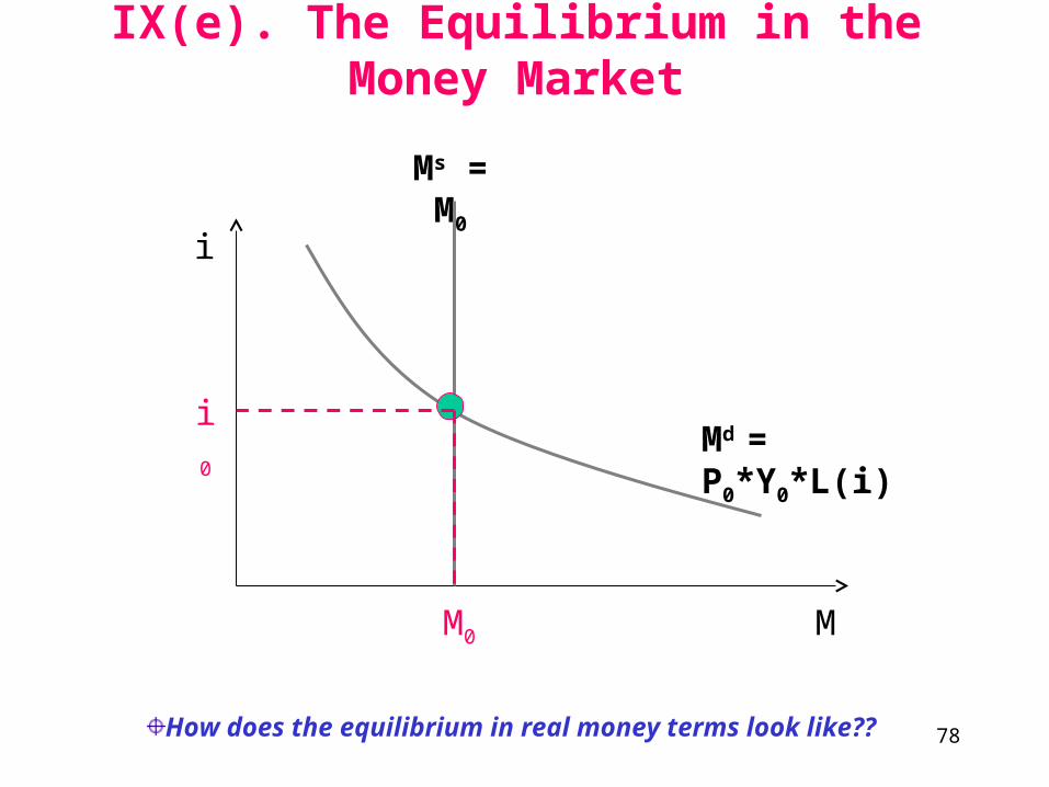
M

i

Md = P0*Y0*L(i)

How does the equilibrium in real money terms look like??

IX(e). The Equilibrium in the Money Market

Ms = M0

M0

i0

79

IX(f). The Interest rate determination in the money market

80

IX(g) The derivation of the LM curve

81

IX(h). Shifts of the LM curve

82

X. IS-LM

a) IS/LM: Effects of a tax increase

b) IS/LM: Effects of a monetary expansion

c) IS/LM: Clinton-Greenspan mix and policy coordination

d) IS/LM: Dynamic effects of monetary contraction

e) Fiscal and monetary efficacy

83

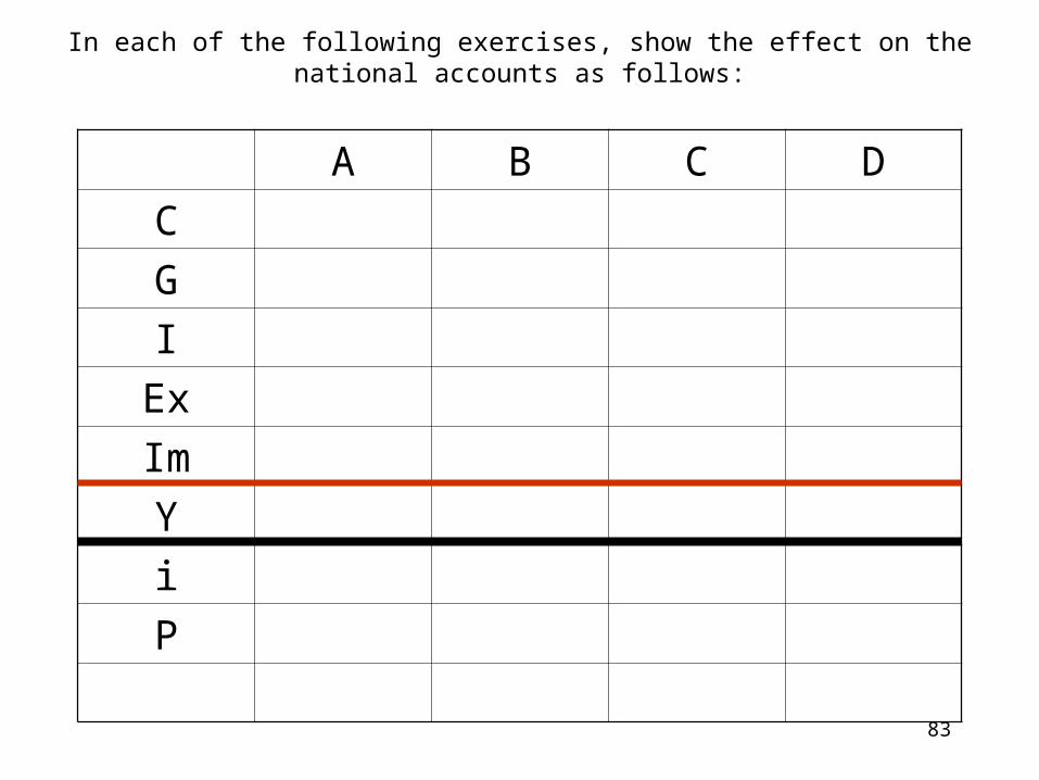
In each of the following exercises, show the effect on the national accounts as follows:

A B C D

C

G

I

Ex

Im

Y

i

P

84

X(a). IS/LM: Effects of a tax increase

85

X(b). IS/LM: Effects of a monetary expansion

86

X(c). IS/LM: Clinton-Greenspan mix and policy coordination

87

X(d). IS/LM: Dynamic effects of monetary contraction

88

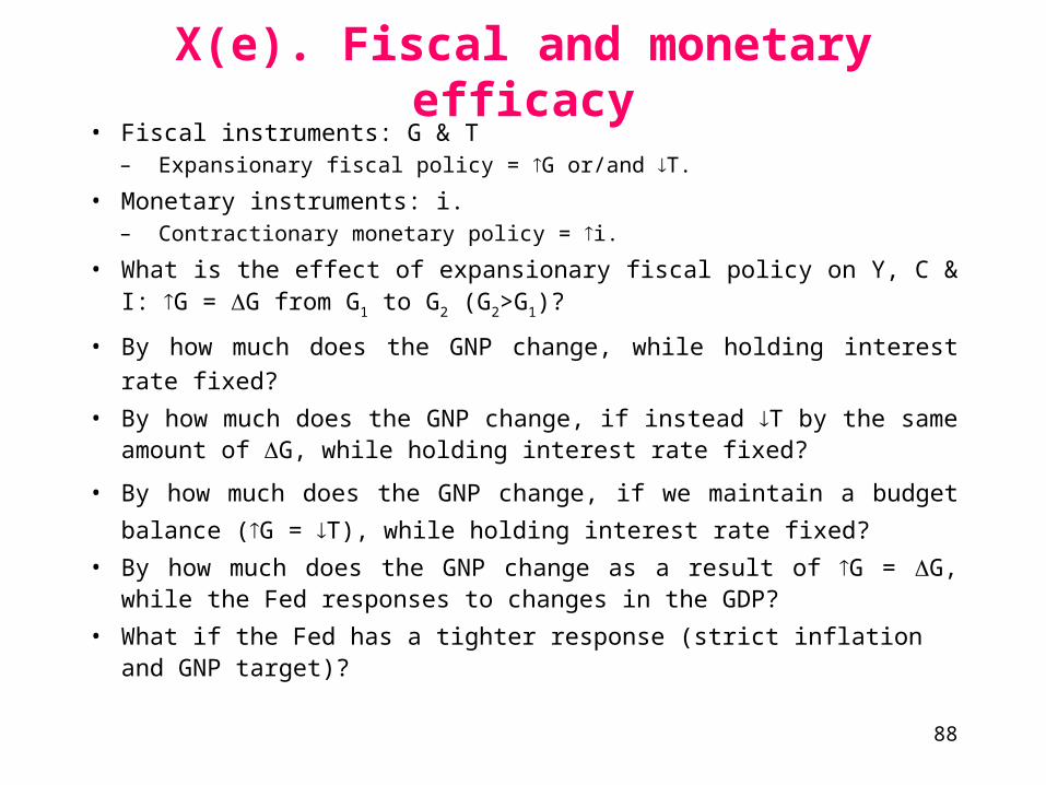
X(e). Fiscal and monetary efficacy• Fiscal instruments: G & T

– Expansionary fiscal policy = G or/and T.

• Monetary instruments: i.– Contractionary monetary policy = i.

• What is the effect of expansionary fiscal policy on Y, C & I: G = G from G1 to G2 (G2>G1)?

• By how much does the GNP change, while holding interest rate fixed?

• By how much does the GNP change, if instead T by the same amount of G, while holding interest rate fixed?

• By how much does the GNP change, if we maintain a budget balance (G

= T), while holding interest rate fixed?

• By how much does the GNP change as a result of G = G, while the Fed responses to changes in the GDP?

• What if the Fed has a tighter response (strict inflation and GNP target)?

89

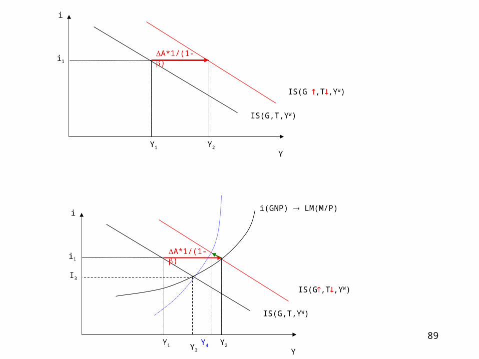
i

Y

IS(G,T,YW)

IS(G ,T,YW)

A*1/(1-)

Y2Y1

i1

i

Y

IS(G,T,YW)

IS(G,T,YW)

A*1/(1-)

i(GNP) LM(M/P)

Y2Y1 Y3

i1

I3

Y4

90

Conclusions:

• Deficit Reduction will change the economy, but it might not boost the unemployment enough due to strict Fed inflationary target.

• Fiscal expansionary policy might be offset by contractionary monetary policy.

• Contrary to what is often stated by politicians, a reduction in the budget does not necessarily lead to an increase in investment.

• The flatter IS (high sensitivity of output to interest rate) the more effective the monetary policy (need small changes in interest rate to achieve the same change in output).

• The steeper LM (strict inflation target by the Fed) the less effective the monetary policy (changes in G or T have less affect on changing the output).

91

XI. Labor Market

a) Overview

b) Some world wide facts

c) Definitions

d) Wage setting equation

e) Price setting equation

f) Equilibrium in the labor market and the natural rate of unemployment

g) Equilibrium unemployment and Output

92

XI(a) Overview

A good measurement for growth of the standard of living is: the real output per capita: RGNP/pop.

(USA2000=$40,000 per year).

In order to have growth, we need to invest in capital.

Investing in capital = accumulating durable productive goods (like machines, hardware and software) and knowledge (R&D and human capital). It does not include financial investment.

Which also means forfeiting current consumption (saving) for higher future consumption. Therefore, investments must be equal to savings. Investing in education may also mean lower current production for higher future production.

93

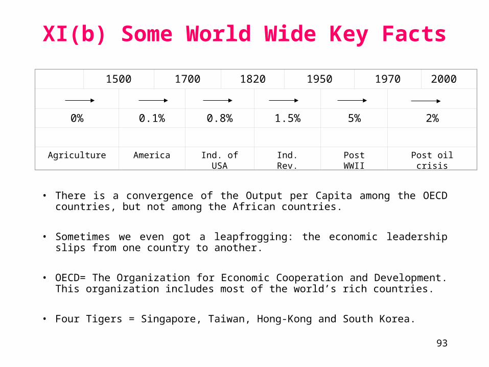
XI(b) Some World Wide Key Facts

• There is a convergence of the Output per Capita among the OECD countries, but not among the African countries.

• Sometimes we even got a leapfrogging: the economic leadership slips from one country to another.

• OECD= The Organization for Economic Cooperation and Development. This organization includes most of the world’s rich countries.

• Four Tigers = Singapore, Taiwan, Hong-Kong and South Korea.

  1500 1700 1820 1950 1970 2000

       

0% 0.1% 0.8% 1.5% 5% 2%

           Agriculture America Ind. of USA Ind. Rev. Post WWII Post oil crisis

94

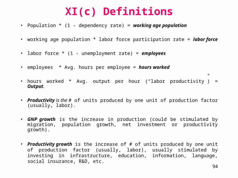
XI(c) Definitions• Population * (1 - dependency rate) = working age population

• working age population * labor force participation rate = labor force

• labor force * (1 - unemployment rate) = employees

• employees * Avg. hours per employee = hours worked

• hours worked * Avg. output per hour (“labor productivity”) = Output.

• Productivity is the # of units produced by one unit of production factor (usually, labor).

• GNP growth is the increase in production (could be stimulated by migration, population growth, net investment or productivity growth).

• Productivity growth is the increase of # of units produced by one unit of production factor (usually, labor), usually stimulated by investing in infrastructure, education, information, language, social insurance, R&D, etc.

95

• Two kinds of unemployed:– Voluntary unemployed: as in searching for a job at a wage higher than they or their

peers are being offered: not a sign of dis-equilibrium (UVOL)

– Involuntary unemployed: actively searching for a job and would accept the prevailing wage, but no offer forthcoming labor supply greater than demand at the prevailing wage Involuntary unemployment creates pressure for (real) wages to fall. (U - UVOL)

• Labor force (Ld) = Employees (N) + Involuntary unemployed (U - UVOL).

• Labor supply (Ls) = the total labor units (monthly, weekly or yearly working hours or jobs) offered for a given real wage, other things equal.

• Unemployment rate (u) = (U - UVOL) / L

• Non-employment rate = U/L

• Participation rate = L / Population of working age

U often comes hand on hand with low participation rate.U.S. (u = 4%, pr = 80% ) France (u=13%, pr = 65%)

• Separation negatively depends on age: experience, education level, skill, seniority, social security and family responsibility.

96

The US CPS

97

• Employees care about their wages’ purchasing power of products. Therefore, what is important for them is their real wage -W/P .

• When unemployment is low, then (a) Workers have more bargaining power, and (b) employers are more anxious to pay higher “efficiency wages” (Ford in 1914). Therefore, real and nominal wages are negatively correlated with unemployment rate.

U Workers are worse-off because (a) probability of losing a job (it’s easier now for the firms to find a replacement), and (b) probability of finding a job (more workers are now competing). Therefore, real and nominal wages are negatively correlated with unemployment rate.

• Most wages are having rigidities for some length of time (a year or more) due contracts (wages are pre-set in advance). Therefore, nominal wages depend on expected prices (forward looking).

• There is a reservation real wage, under which workers won’t consider any offer to work. Therefore, real wages are always above this floor.

• Other factors that affect real wages include: productivity, unemployment benefits, experience, education level, skill, seniority, social security.

XI(d) Wage setting equation

98

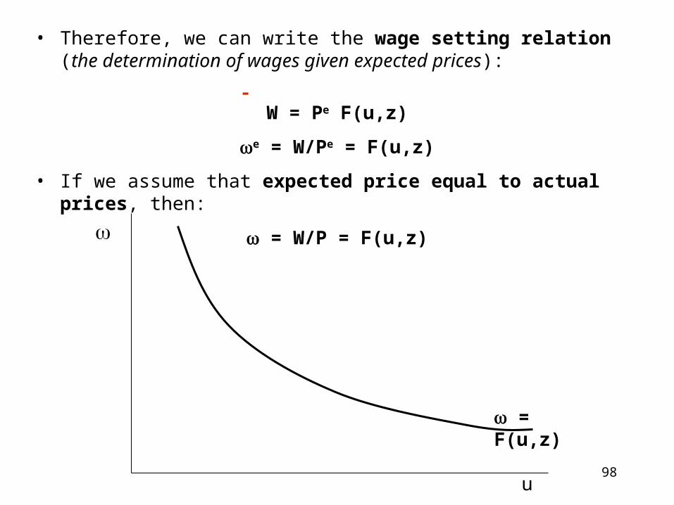
• Therefore, we can write the wage setting relation (the determination of wages given expected prices):

-W = Pe F(u,z)

e = W/Pe = F(u,z)

• If we assume that expected price equal to actual prices, then:

= W/P = F(u,z)

= F(u,z)

u

99

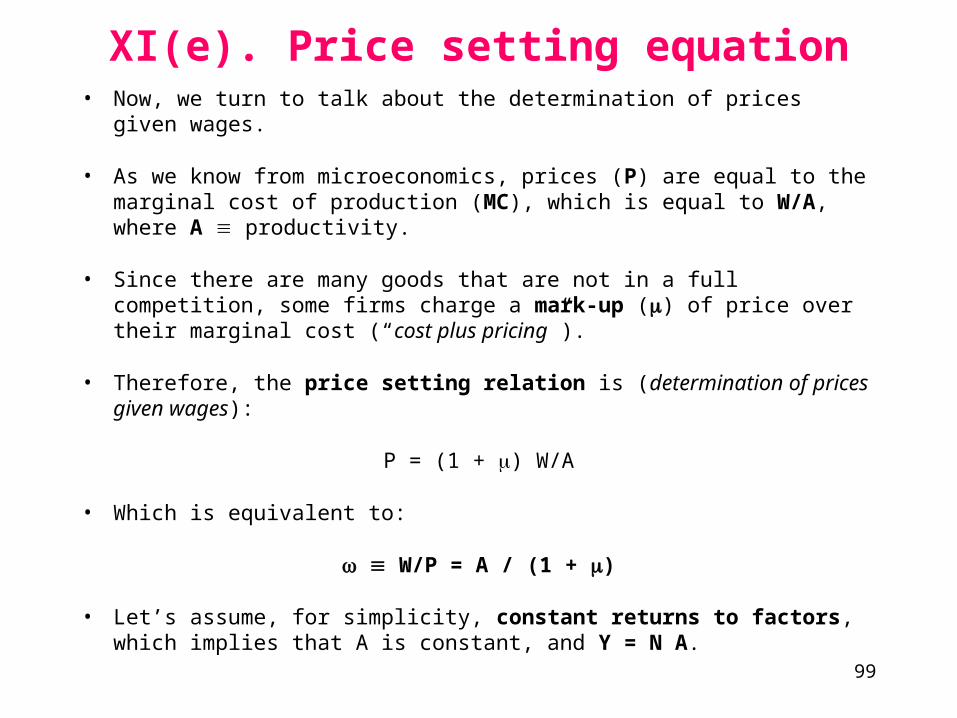
XI(e). Price setting equation• Now, we turn to talk about the determination of prices given wages.

• As we know from microeconomics, prices (P) are equal to the marginal cost of production (MC), which is equal to W/A, where A productivity.

• Since there are many goods that are not in a full competition, some firms charge a mark-up () of price over their marginal cost (“cost plus pricing”).

• Therefore, the price setting relation is (determination of prices given wages):

P = (1 + ) W/A

• Which is equivalent to:

W/P = A / (1 + )

• Let’s assume, for simplicity, constant returns to factors, which implies that A is constant, and Y = N A.

100

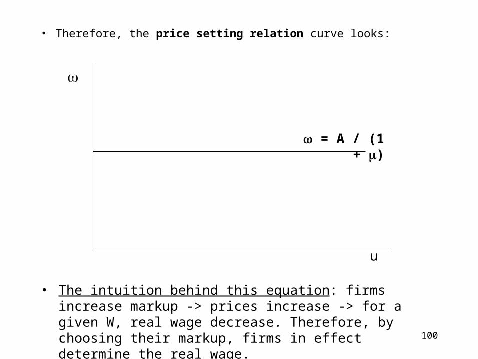
• Therefore, the price setting relation curve looks:

= A / (1 + )

u

• The intuition behind this equation: firms increase markup -> prices increase -> for a given W, real wage decrease. Therefore, by choosing their markup, firms in effect determine the real wage.

101

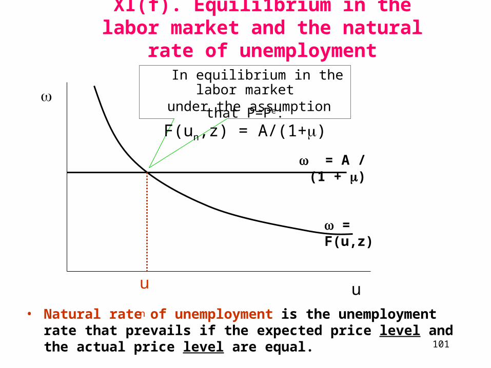
XI(f). Equili1brium in the labor market and the natural rate of unemployment

• Natural rate of unemployment is the unemployment rate that prevails if the expected price level and the actual price level are equal.

= A / (1 + )

u

= F(u,z)

un

In equilibrium in the labor market under the assumption that P=Pe:

F(un,z) = A/(1+)

102

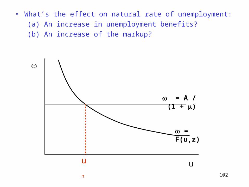
• What’s the effect on natural rate of unemployment:

(a) An increase in unemployment benefits?

(b) An increase of the markup?

= A / (1 + )

u

= F(u,z)

un

103

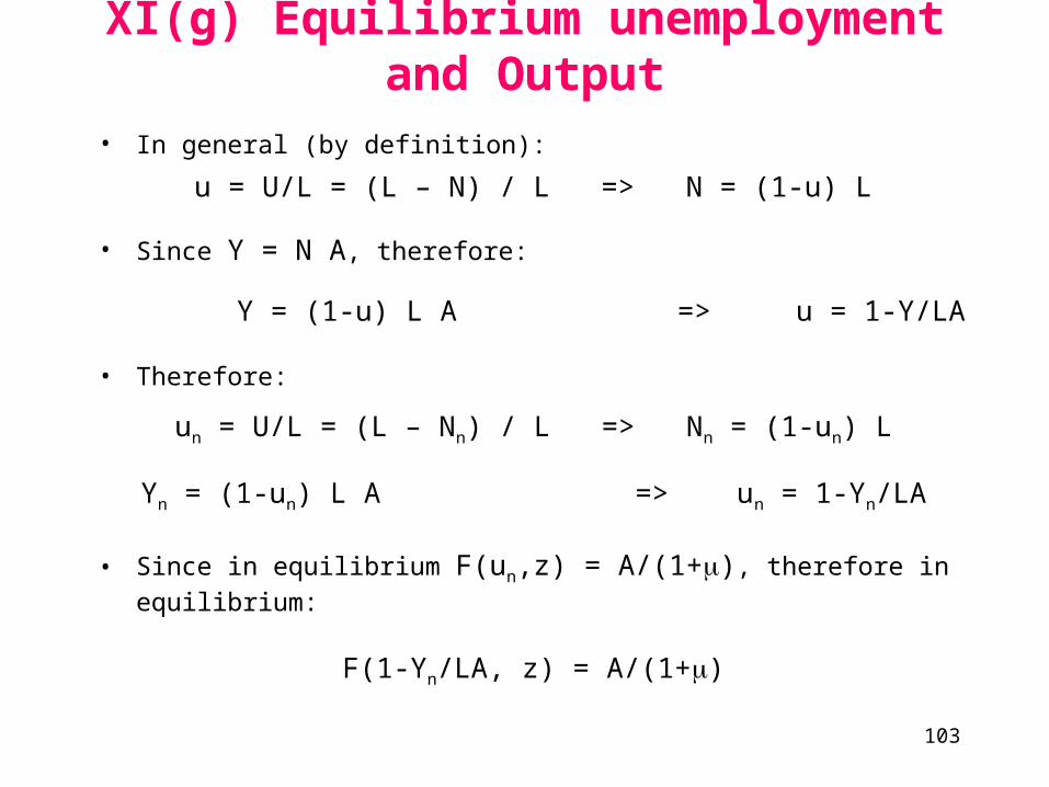
• In general (by definition):

u = U/L = (L – N) / L => N = (1-u) L

• Since Y = N A, therefore:

Y = (1-u) L A => u = 1-Y/LA

• Therefore:

un = U/L = (L – Nn) / L => Nn = (1-un) L

Yn = (1-un) L A => un = 1-Yn/LA

• Since in equilibrium F(un,z) = A/(1+), therefore in equilibrium:

F(1-Yn/LA, z) = A/(1+)

XI(g) Equilibrium unemployment and Output

104

The Medium Run

a) AD- definition & derivation

b) AS- definition & derivation

c) General equilibrium in the medium run- definition & derivation

105

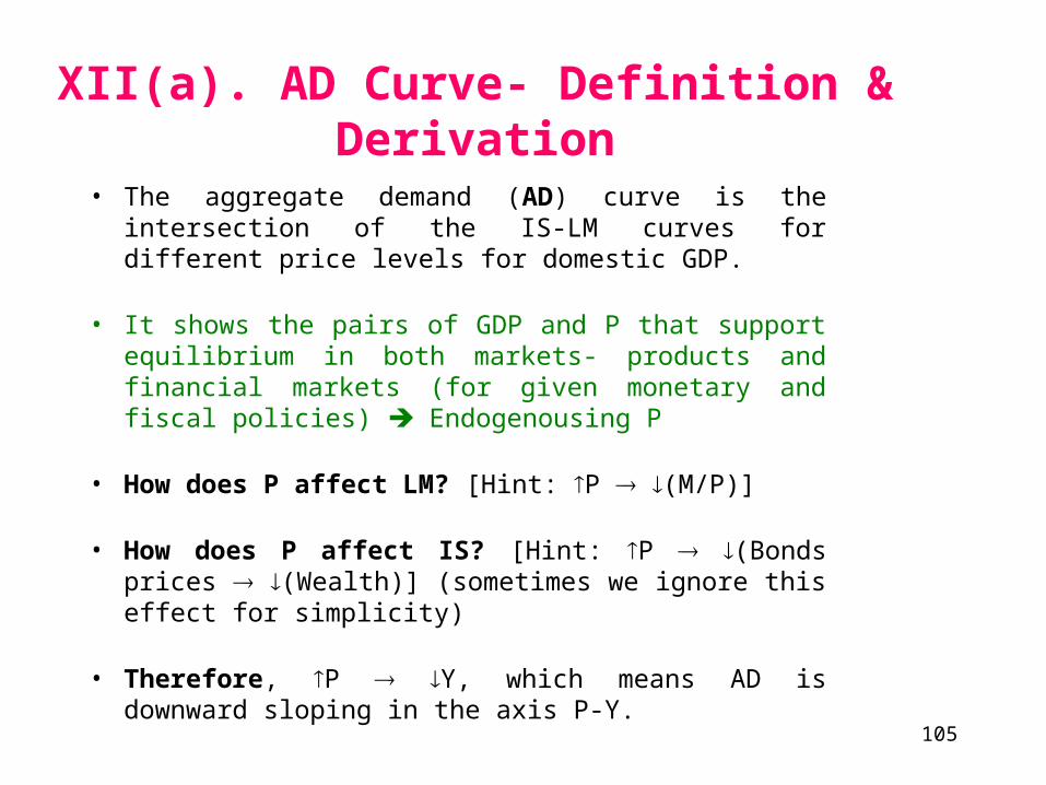
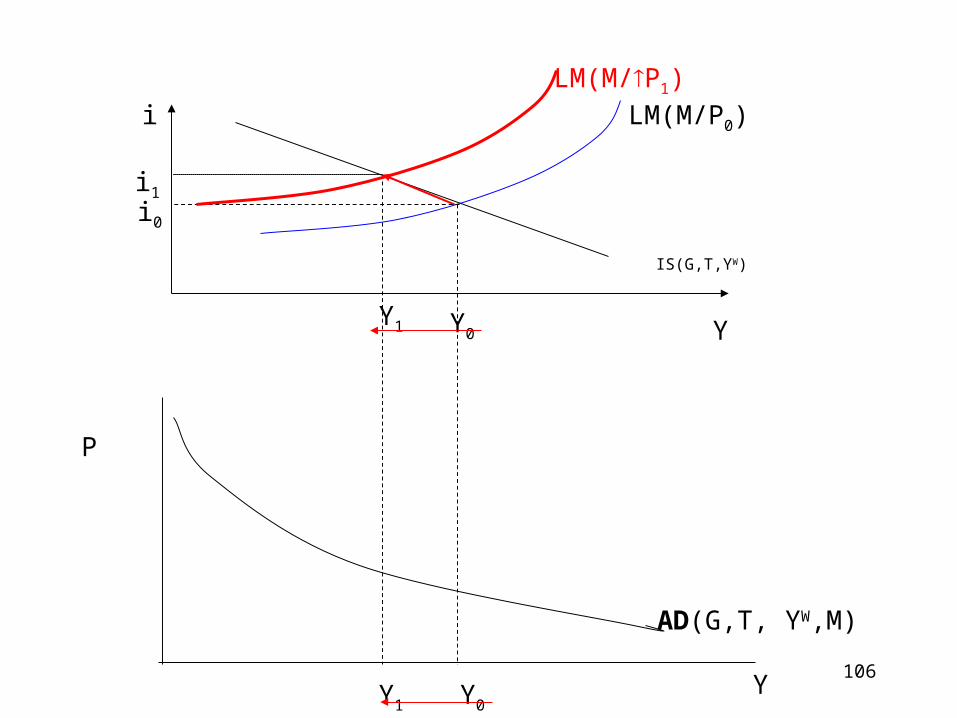
XII(a). AD Curve- Definition & Derivation

• The aggregate demand (AD) curve is the intersection of the IS-LM curves for different price levels for domestic GDP.

• It shows the pairs of GDP and P that support equilibrium in both markets- products and financial markets (for given monetary and fiscal policies) Endogenousing P

• How does P affect LM? [Hint: P (M/P)]

• How does P affect IS? [Hint: P (Bonds prices (Wealth)] (sometimes we ignore this effect for simplicity)

• Therefore, P Y, which means AD is downward sloping in the axis P-Y.

106

i

Y

IS(G,T,YW)

LM(M/P1)

Y1 Y0

i1

i0

LM(M/P0)

AD(G,T, YW,M)

P

YY1 Y0

107

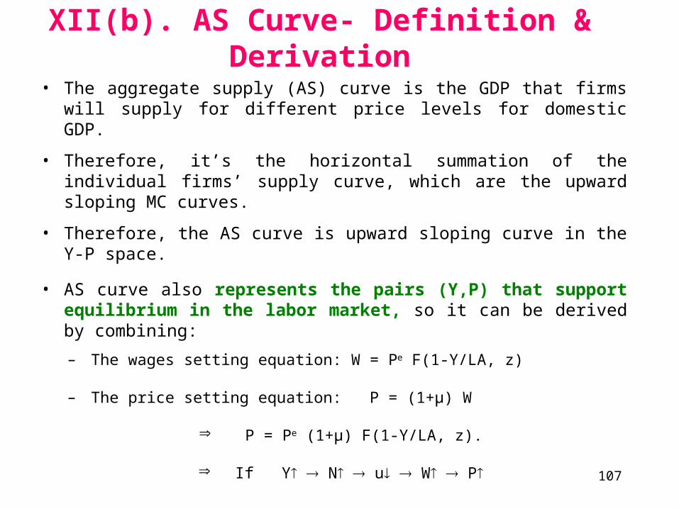
XII(b). AS Curve- Definition & Derivation

• The aggregate supply (AS) curve is the GDP that firms will supply for different price levels for domestic GDP.

• Therefore, it’s the horizontal summation of the individual firms’ supply curve, which are the upward sloping MC curves.

• Therefore, the AS curve is upward sloping curve in the Y-P space.

• AS curve also represents the pairs (Y,P) that support equilibrium in the labor market, so it can be derived by combining:

– The wages setting equation: W = Pe F(1-Y/LA, z)

– The price setting equation: P = (1+µ) W

P = Pe (1+µ) F(1-Y/LA, z).

If Y N u W P

108

AS(Pe,PK,,Tech, Competition, A, ..)

P

YYn

Pe

Y’

P’

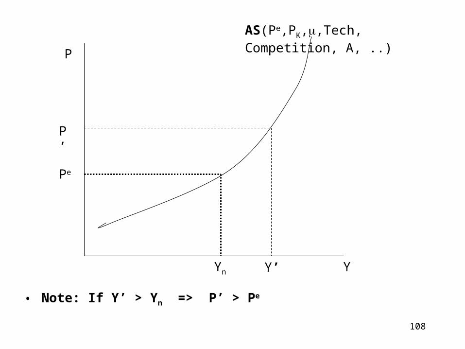
• Note: If Y’ > Yn => P’ > Pe

109

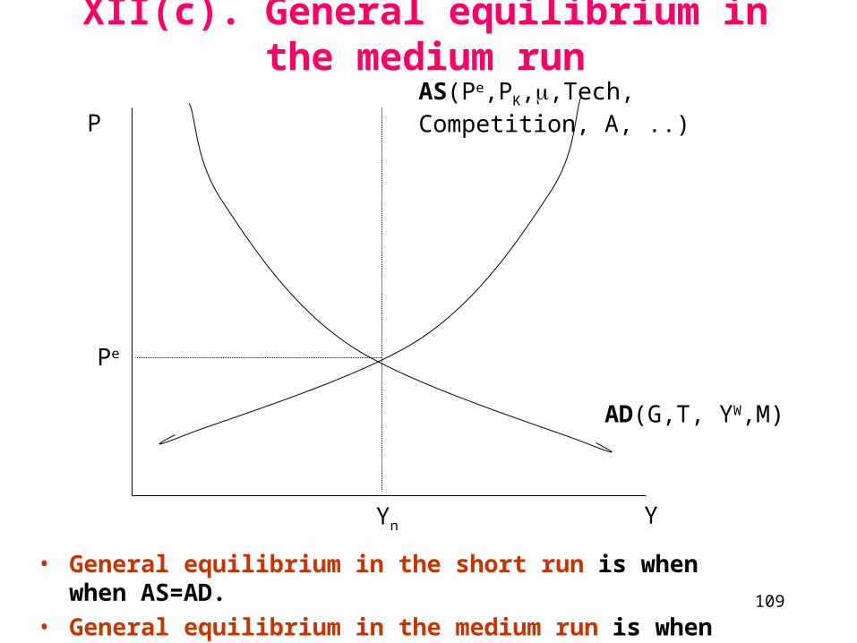
XII(c). General equilibrium in the medium runAS(Pe,PK,,Tech, Competition, A, ..)

P

Y

AD(G,T, YW,M)

Yn

Pe

• General equilibrium in the short run is when when AS=AD.

• General equilibrium in the medium run is when AS=AD at Y=Yn (or equivalently, at P=Pe)

110

AS(Pe0,PL,,Tech)

P

Y

AD(G,T, YW,M)

AD’(G,T, YW, M)

Y1Yn

P1

Pe0

Pe2

XII(d). Money neutrality in the medium run

A

D

C

B

AS’’(Pe2)

111

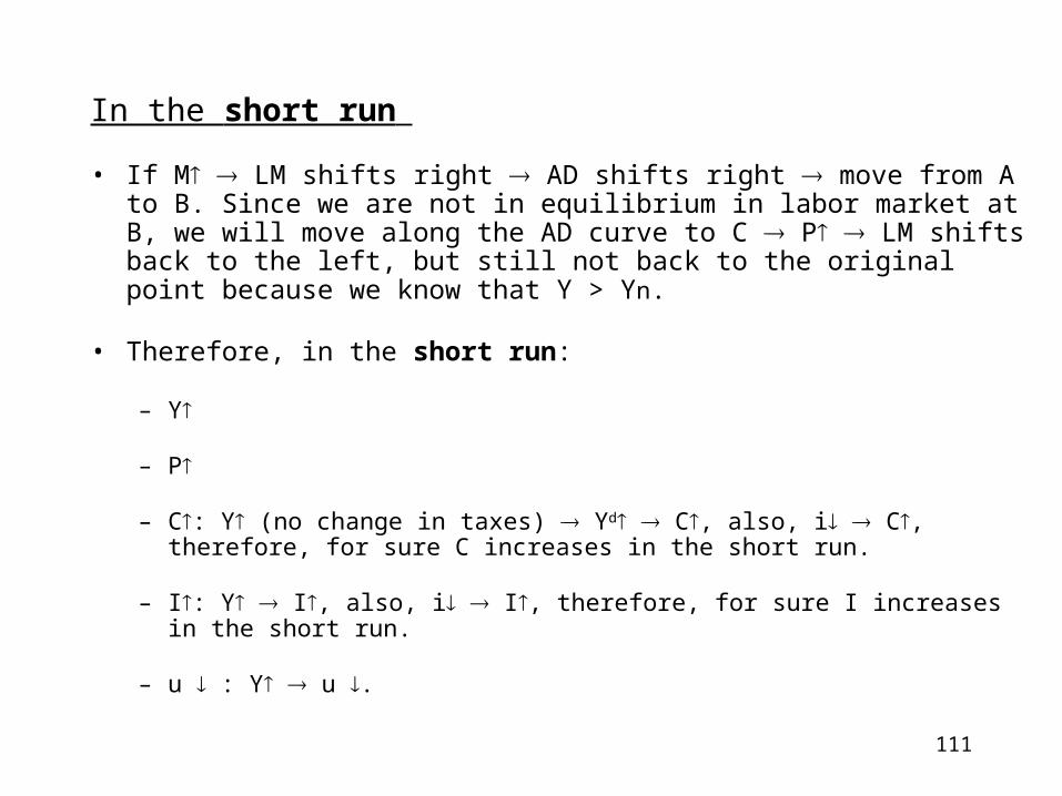
In the short run

• If M LM shifts right AD shifts right move from A to B. Since we are not in equilibrium in labor market at B, we will move along the AD curve to C P LM shifts back to the left, but still not back to the original point because we know that Y > Yn.

• Therefore, in the short run:

– Y

– P

– C: Y (no change in taxes) Yd C, also, i C, therefore, for sure C increases in the short run.

– I: Y I, also, i I, therefore, for sure I increases in the short run.

– u : Y u .

112

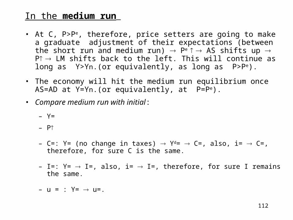
In the medium run

• At C, P>Pe, therefore, price setters are going to make a graduate adjustment of their expectations (between the short run and medium run) Pe AS shifts up P LM shifts back to the left. This will continue as long as Y>Yn.(or equivalently, as long as P>Pe).

• The economy will hit the medium run equilibrium once AS=AD at Y=Yn.(or equivalently, at P=Pe).

• Compare medium run with initial:

– Y=

– P

– C=: Y= (no change in taxes) Yd= C=, also, i= C=, therefore, for sure C is the same.

– I=: Y= I=, also, i= I=, therefore, for sure I remains the same.

– u = : Y= u=.

113

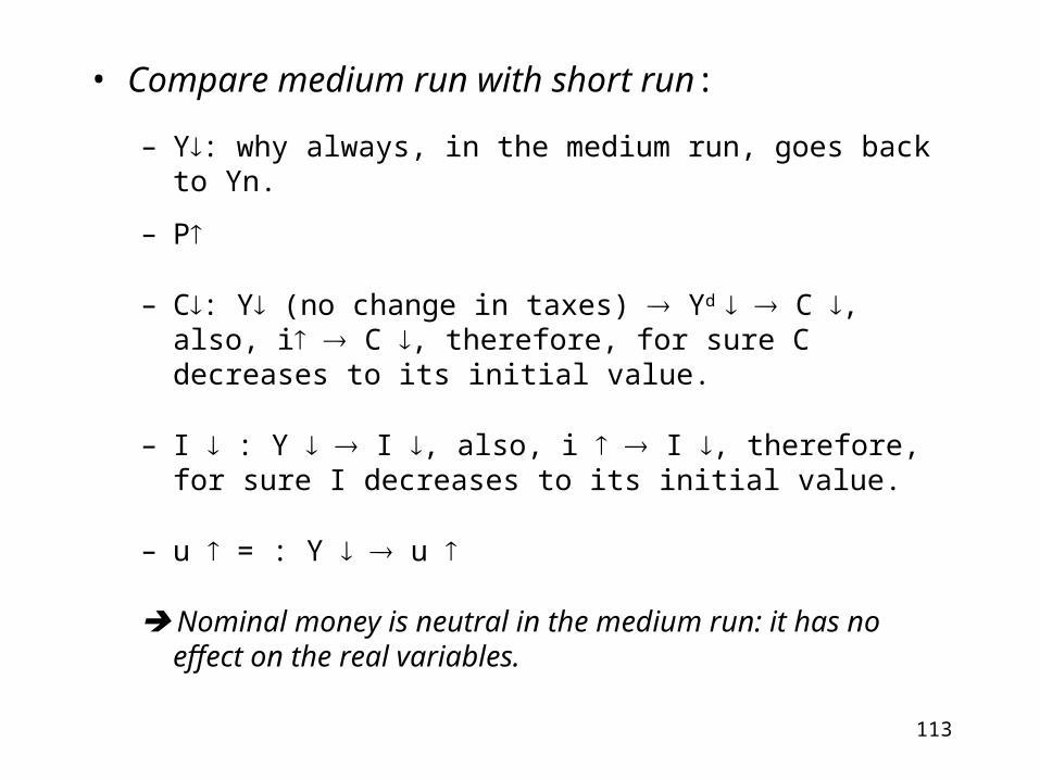
• Compare medium run with short run:

– Y: why always, in the medium run, goes back to Yn.

– P

– C: Y (no change in taxes) Yd C , also, i C , therefore, for sure C decreases to its initial value.

– I : Y I , also, i I , therefore, for sure I decreases to its initial value.

– u = : Y u

Nominal money is neutral in the medium run: it has no effect on the real variables.

114

• Does a fiscal expansion has the same results? No. (Hint: The aggregate demand in the new medium run equilibrium is the same (equal to Yn); however, the combination is now different:

Yn = C(Y=,i) + G + I(Y=,i)

XII(d). Fiscal policy’s effect in the medium run

115

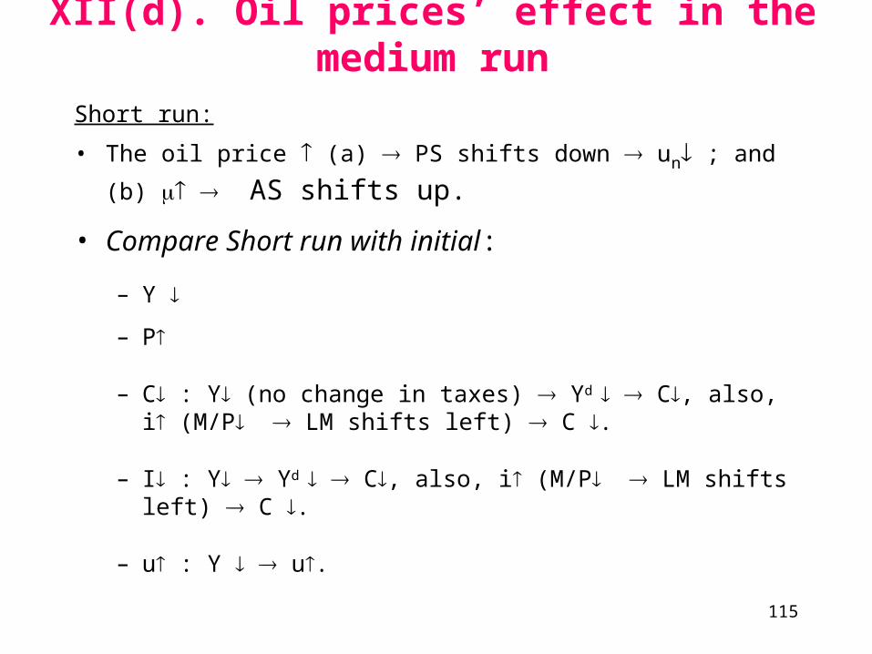
Short run:

• The oil price (a) PS shifts down un ; and (b) AS shifts up.

• Compare Short run with initial:

– Y

– P

– C : Y (no change in taxes) Yd C, also, i (M/P LM shifts left) C .

– I : Y Yd C, also, i (M/P LM shifts left) C .

– u : Y u.

XII(d). Oil prices’ effect in the medium run

116

Medium run:

• P>Pe, therefore, price setters are going to make a graduate adjustment of their expectations (between the short run and medium run) Pe AS shifts up P LM shifts left. This will continue as long as Y> new Yn.(or equivalently, as long as P>Pe):

• Compare medium run with initial:

– Y

– P

– C : Y (no change in taxes) Yd C, also, i (M/P LM shifts left) C .

– I : Y Yd C, also, i (M/P LM shifts left) C .

– u : Y u.

Yn = C(Y=,i) + G + I(Y=,i)

117

Inflation and Phillips Curve

118

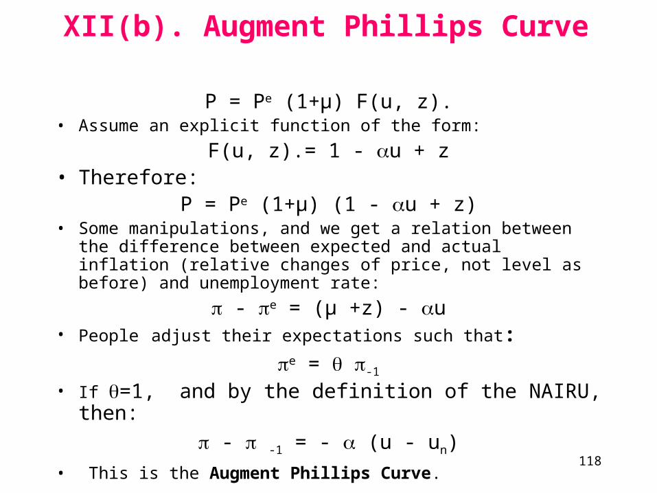
P = Pe (1+µ) F(u, z).• Assume an explicit function of the form:

F(u, z).= 1 - u + z• Therefore:

P = Pe (1+µ) (1 - u + z)• Some manipulations, and we get a relation between the difference

between expected and actual inflation (relative changes of price, not level as before) and unemployment rate:

- e = (µ +z) - u• People adjust their expectations such that:

e = -1

• If =1, and by the definition of the NAIRU, then:

- -1 = - (u - un)

• This is the Augment Phillips Curve.

XII(b). Augment Phillips Curve

119

• Note:• When =0, we get the original Philips curve, a relation between the

level of inflation rate and the level of involuntary unemployment rate, which prevailed until the 1950s.

• When =1, we get the accelerationist Philips curve (or modified or expectations-augmented Philips curve), a relation between the change in the inflation rate and level of the involuntary unemployment rate, which prevailed since the 1960s.

• Higher expected inflation leads to higher inflation.

• The higher the mark-up and the factors affect wage determination, the higher the inflation

120

• In general, we can state the Okun’s law:

ut – ut-1 = [gy(avg) – gy(t)]

• There is a cyclical relation between unemployment and real growth: The change in the unemployment is half the growth rate difference between potential and actual GDP growth. Or, the level of unemployment is half the % gap of the potential and actual GDP.

XII(c). Okun’s Law

121

The Long Run

a) Facts about growth

b) Aggregate production function

c) Example

122

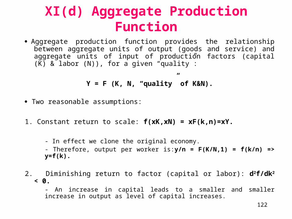
XI(d) Aggregate Production Function

Aggregate production function provides the relationship between aggregate units of output (goods and service) and aggregate units of input of production factors (capital (K) & labor (N)), for a given “quality”:

Y = F (K, N, “quality” of K&N).

 Two reasonable assumptions:

1. Constant return to scale: f(xK,xN) = xF(k,n)=xY.

- In effect we clone the original economy.- Therefore, output per worker is:y/n = F(K/N,1) = f(k/n) => y=f(k).

2.   Diminishing return to factor (capital or labor): d2f/dk2 < 0.- An increase in capital leads to a smaller and smaller increase in output as level of capital increases.

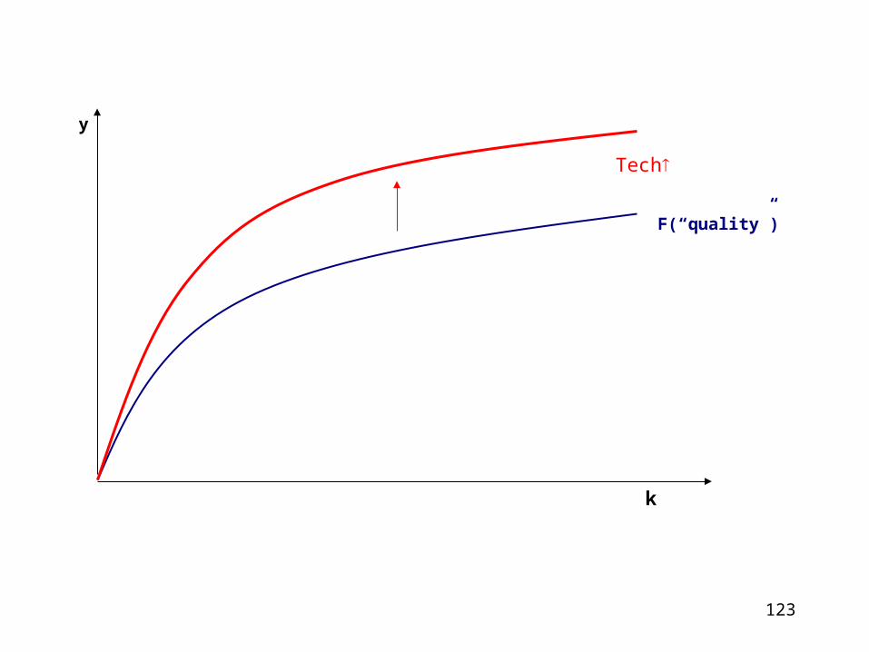
123

k

y

F(“quality”)

Tech