MTL TR 88-46 AD

0o A COMBINED ISOTROPIC-KINEMATIC< HARDENING MODEL FOR LARGEcDEFORMATION METAL PLASTICITY

CHARLES S. WHITEMATERIALS DYNAMIC BRANCH

December 1988

Approved for public release; distribution unlimited. OTIC:- ECTE0

E

US ARMYLABORATORY COMMAND U.S. ARMY MATERIALS TECHNOLOGY LABORATORYMATEnuaL TECH0LOGY LAIATOR Watertown, Massachusetts 02172-0001

The findings in this report are not to be construed as an officialDepartment of the Army position, unless so designated by otherauthorized documents.

Mention of any trade names or manufacturers in this reportshall not be construed as advertising nor as an officialindorsement or approval of such products or companies bythe Lited States Government.

0ISPOSITION INSTRUCTIONS

Oestrov this report when it is no longer nmeded.DO not return it to the originator.

UNCLASSIFIEDSECURITY CLASSIFICATION Of THIS PAGE (When Does Entered)

REPORT DOCUMENTATION PAGE READ INSTRUCTIONSBEFORE COMPLETING FORM

.REPORT NUMSER 2. GOVT ACCESSION NO. 3. RECIPIENT'S CATALOG NUMBER

MTL TR 88-46 1

4. TITLE (and Subtie) S. TYPE OF REPORT & PERIOD COVERED

A COMBINED ISOTROPIC-KINEMATIC HARDENING MODEL Final Report

FOR LARGE DEFORMATION METAL PLASTICITY 6. PERFORMING ORG. REPORT NUMBER

7. AUTHOR(s) S. CONTRACT OR GRANT NUMBER(s)

Charles S. White

9. PERFORMING ORGANIZATION NAME AND ADDRESS 10. PROGRAM ELEMENT. PROJECT. TASKAREA & WORK UNIT NUMBERS

U.S. Army Materials Technology LaboratoryWatertown, Massachusetts 02172-0001 D/A Project: IL263102D077ATTN: SLCMT-MRD_

11. CONTROLLING OFFICE NAME AND ADDRESS 12. REPORT DATE

U.S. Army Laboratory Command December 1988

2800 Powder Mill Road 13. NUMBEROFPAGES

Adelphi, Maryland 20783-1145 24814. MONITORING AGENCY NAME & AOORESS(if dlllerent from Controlling Office) IS. SECURITY CLASS. (of this report)

Unclassified15. OECL ASSI FIC ATION/DOWN GRADING

SCHEDULE

16. DISTRIBUTION STATEMENT (of this Report)

Approved for public release; distribution unlimited. D T. G

17. DISTRIBUTION STATEMENT (of the abstract entered in Block 20. it different from Report) N 198

II. SUPPLEMENTARY NOTES

Submitted to the Department of Mechanical Engineering, MIT, in partial ful-fillment of the requirements for the Degree of Doctor of Philosophy in

Mechanical Engineering.

I. KEY VfPROS (Continue on reverse side if necessary md Identify by block number)

Plastic properties I Stainless steel Mathematical models,Plastic deformation Aluminum ? Stress strain relations )

Metals Carbon steels Strain hardeningN

20. ABSTRACT (Continue on reverse side It necessary and Identify by block number)

(SEE REVERSE SIDE)

D I FORm 1473 EDITION OF I NOV 65 IS OBSOLETE T UNCLASS I FIGEDSECURITY CLASSIFICATION Of THIS PAGE (When Date Entered)

UNCLASSIFIEDSECURITY CLASSIFICATION OF THIS PAGE Whon D.ra Fnre.d)

Block io. 20

ABSTRACT

The need for increased accuracy in material modeling has been driven inrecent years by advances in computing capability and the complexity of problemswhich now may be analyzed. Current material models are unable to represent manyof the important multi-dimensional effects of the plastic deformation of metals tolarge strain. These effects can become very important at the level of deformationreached in metal processing operations, shear band formation, penetration mecha-nisms, and crack tip processes.

An experimental program was conducted to produce a number of different typesoi tests on several materials. The types of tests included: tension, large straincompression, symmetric cyclic, unsymmetric cyclic, single reverse and large straintorsion. Materials tested were type 316 stainless steel and 1100-0 aluminum. Alsodata for 3 carbon steels was analyzed. \

A new constitutive model for metal deformation is introduced to analyze andpredict these experiments. The model contains both isotropic and kinematic hard-ening components but overcomes some of the shortcomings of previous such models byintroducing new material functions. The two important new features are: 1) Theback stress moduli depend upon the position of the back stress within a surfacedefined by its previous maximum norm, and 2) During a reversing event the isotropiccomponent initially softens. The effects of these features are discussed andimplemented using simple functions in the constitutive model.

The model captures key features of small strain uniaxial cyclic behavior verywell including the additional hardening due to nonproportional cycling in tension-torsion. The predictions of the finite torsion results are not as close. Theinclusion of plastic spin does not affect these results.

II

2 UNCLASSIFIEDSECURITY CLASSIFICATION OF THIS PAGE IWN.n ifeAa Fnteedj

Preface

The research presented in this report was carried out at the U.S. Army Mate-

rials Technology Laboratory and at the Massachusetts Institute of Technology in

Cambridge, Massachusetts.

This report is excerpted from the Ph.D. thesis of the author and was completed

in August, 1988 in the Department of Mechanical Engineering at the Massachusetts

Institute of Technology. The thesis was supervised by Professor Lallit Anand of the

Department of Mechanical Engineering at MIT. Also serving on the thesis advisory

committee were Professors David M. Parks and Klaus-Jurgen Bathe of MIT and

Dr. Dennis M. Tracey of MTL.

El

. ., .-- Codes:', i. ane/or r,,-

.D$,,t i .Sjocia lPcn

4

3

Table of Contents

1. Introduction .............................................................. 8

2. Review of the Bauschinger Effect ..................................... 12

2.1 Scope of Chapter ..................................................... 12

2.2 Review of the Literature .............................................. 12

2.3 Sum m ary ............................................................ 32

3. Micromodeling of a Particle-Hardened Alloy Using the Finite ElementM ethod .................................................................. 40

3.1 Axisymmetric Unit Cell Model ....................................... 42

3.2 Plane Strain Unit Cell Model ......................................... 50

3.2.1 Tensile Loading .................................................. 51

3.2.2 Sim ple Shear ..................................................... 53

4. Review of Plasticity Modeling ......................................... 73

4.1 Experimental Review ................................................. 74

4.1.1 Large Strain ..................................................... 74

4.1.2 Cyclic Plasticity .................................................. 75

4.2 Review of Constitutive Modeling ..................................... 80

5

4.2.1 Large Strain Extensions of Previous Theories ..................... 80

4.2.2 Theories for Cyclic Plasticity ..................................... 86

5. Constitutive Equations for Rate-Independent, Elastic-Plastic Solids 97

5.1 Overview ............................................................. 97

5.2 Finite Deform ation ................................................... 97

5.3 Function Dependence ................................................ 100

5.4 Functional Dependence .............................................. 104

5.4.1 Back Stress Evolution ........................................... 104

5.4.2 Isotropic Hardening ............................................. 107

6. Experimental Program ................................................ 111

6.1 Types of Experiments ............................................... 111

6.2 M aterials Tested .................................................... 112

6.3 Experimental Apparatus ............................................ 113

6.4 Compression Testing ................................................ 114

6.5 Reverse Straining Testing ........................................... 116

6.6 Finite Element Analysis of Reverse Straining Specimen .............. 118

6.7 Torsion Testing ..................................................... 121

6.8 Experimental Results ................................................ 126

6.9 Comparison of Some Exis;ing Theories with the Experiments ........ 131

7. Comparison of Theory with Experiments ........................... 164

7.1 Specific Material Functions Employed ............................... 164

7.2 Simple Example of Model Components .............................. 167

7.3 Procedure for Determining Constants ................................ 168

7.4 Correlation of Theory with Base Experiments ........................ 173

7.5 Evaluation of the Predictive Capability of the Model ................. 174

7.5.1 Symmetric Strain Cycling ....................................... 175

7.5.2 Unsymmetric Strain Cycling .................................... 176

7.5.3 Unsymmetric Stress Cycling ..................................... 177

7.5.4 900 Out-of-Phase Cycling ....................................... 178

7.5.5 Fixed End Torsion Tests ........................................ 180

8. C onclusions ............................................................ 214

R eferences .............................................................. 219

A ppendix A ............................................................ 232

A ppendix B ............................................................ 240

7

Chapter 1

Introduction

In recent years there has been an increased interest in the formulation of finite

deformation, elastoplastic, constitutive equations. Current material models are

unable to represent many of the important multi-dimensional effects of the plastic

deformation of metals to large strain. These effects can become very important

at the level of deformation reached in metal processing operations, shear band

formation, penetration mechanisms, and crack tip processes.

The great advances in computing capability and numerical procedures in the last

decade have led to a tremendous increase in the types and complexity of problems

which may be now analyzed. The computer revolution has far outstripped the

precision of available material models. Previously, a first order prediction from

simple constitutive equations was thought to be sufficient since that coincided with

the accuracy of the available anaylsis techniques. Now the material models greatly

lag our ability to apply them in analysis.

One reason that constitutive development has suffered is the limited experimen-

tal data available to describe large strain behavior. Even more important than the

volume of data available is the type. Pure uniaxial information is not sufficient

8

when many of the discrepancies of the classical theories derive from their tensorial

generalizations. Chief among these phenomena are the differences between material

behavior in tension/compression and in torsion. When comparing the Mises equiv-

alent stress versus equivalent strain curves for torsion and compression, the results

are seen to differ. The torsion results generally fall below the compression results.

Attempts to model this, and other findings, have led some to consider variations

of the classical kinematic hardening plasticity law. These efforts have illustrated

problems that arise when simple, small strain, constitutive laws are hastily gener-

alized to the finite deformation regime. The most notable of these is the prediction

of an oscillating shear stress response for monotonic loading in simple shear.

Many authors have considered this problem from an analytical point-of-view over

the past five years. Consequently, many theories or constitutive assumptions have

been postulated. None of these have been properly investigated experimentally. A

consistent and complete experimental data base has not been available for evaluating

the models.

The purpose of this work is to conduct a complete set of experiments, on several

materials, that would allow proper comparisons to be made. This set of experiments

includes, of course, large strain compression and torsion tests. Additionally, it was

realized that a proper model would need to correctly model the back stress or

kinematic hardening as well as the isotropic portion. To aid these determinations,

reverse loading and cyclic experiments were also conducted. These were necessary

to quantify the Bauschinger effect.

The most extensive experimentation and modeling of back stress phenomena is

in the small strain cyclic regime. A proper model of the back stress and its evolution

9

would need to be consistent with the results seen there. Currently none of the large

strain theories correctly model this regime. Different theories have been used by

researchers working in these different regimes. No constitutive model unifying these

different areas has been available.

It is well known that the back stress builds up quickly in the first few percent

strain. This is where most of the action occurs. Its effects can be important at

both small and large strain. A theory which desires to model the effect of the back

stress at large strain needs to also correctly model its behavior at small strain.

This work has two major parts. The first is the experimental results. These

provide a coherent set of tests, useful for plasticity model construction and verifi-

cation. The second is the modeling ideas which allow unification of the different

s rain regimes. These are brought out in a new constitutive model which is applied

to the experimental results.

This document has two main parts, each giving a slightly different perspec-

tive. It is organized in the following way. The first part examines the Bauschinger

Effect from a material scientist's viewpoint. Chapter 2 contains a review of the ex-

perimental literature concerning measurement and description of the Bauschinger

Effect. The quantitative models are not discussed but the causes of the effect are

emphasized. In Chapter 3, micromodeling of the Bauschinger Effect in a particle

hardened alloy is presented. A finite element model was used to model the effects of

the particle-matrix interaction. The results demonstrate many of the experimental

observations of nonmonotonic loading.

The second main part of this document takes a continuum mechanics viewpoint.

The modeling of metal plasticity is reviewed in Chapter 4. A new constitutive

10

model is presented in Chapter 5. It contains new features motivated by the reviews

of the literature. Chapter 6 contains the experimental program and results. The

comparison of the theory with these experiments is given in Chapter 7. Finally, the

conclusions drawn from this study are presented and discussed in Chapter 8.

11

Chapter 2

Review of Bauschinger Effect

2.1 Scope of Chapter

In this chapter the relevant, published work on the anisotropic hardening behav-

ior of metals as exhibited by the Bauschinger Effect is reviewed. This is important

behavior to consider, as will be shown, since the influence of the causes of this behav-

ior have far reaching effects in small strain, cyclic, and large strain metal plasticity.

There exists an extensive literature containing observations of the Bauschinger Ef-

fect. Only a brief review is given here. Major results are listed as well as a review of

some individual investigator's findings. It is valuable to understand the underlying

focus of the studies presented in the literature. This is important when reinterpret-

ing the results of these previous investigators in light of more recent findings. The

summary of this chapter contains some of these new results and how they impact

previous work.

2.2 Review of the Literature

This section is intended to review the experimental measurement of the Bauschinger

effect in metals. It does not include experimental techniques but rather presents ma-

12

jor experimental results in a historical manner leading to the current understanding

of the phenomenon. The Bauschinger effect should not be considered an anomolous

material behavior because it will be shown to be present in a large variety of metals

ranging from pure single crystals to multiphase, polycrystals. The viewpoint of

concern is the phenomenological approach describing macroscopic behavior.

In 1881, Johann Bauschinger [1886] reported that a metal specimen (Bessemer

steel), after receiving an axial extension into the plastic range showed a decrease

in the magnitude of the yield stress upon subsequent compression. This reduction

in yield stress upon reversal of straining is known as the "Bauschinger effect".

This phenomenon has been noted in both rate independent and rate dependent

regimes of material behavior. This review will concentrate on the rate independent

observations since different classes of experiments are required to determine back

stress existence and magnitude in the viscoplastic response regime.

We will also use the term back stress to denote a modeling concept first put

forth by Prager [19561 to describe a multiaxial generalization of this phenomenon

noted in one dimension by Bauschinger. Many of the modern constitutive theories

for elevated temperature structural applications contain back stress variables. For

a review of these applications and a discussion of the modeling of back stress at

elevated temperature see Swearengen and Holbrook [1985].

Just as manifestations of the Bauschinger effect have been seen in the very

slow strain rate (creep) regime, so has it been observed in the high strain rate

regime. Ogawa [1985] demonstrated that the Bauschinger effect at high strain rate

(5 x 102sec- 1 ) has similar features to the quasistatic case. We will not consider the

high strain rate environment separately here.

13

The microscopic approach of requiring the critical shear stress on a slip plane

within a crystal to depend upon the direction of slipping has also been recently

pursued (Weng 119801). These shear components can then be averaged over the

available slip systems to yield the macroscopic behavior of the polycrystalline sam-

ple. Models such as these may lead to increased understanding of the mechanisms

underlying the observed Bauschinger effect but are outside of the domain of the

phenomenological approach and will not be considered in detail here.

The alloy systems which generally show the largest Bauschinger effect, or differ-

ences in yield stresses, is the two phase system where hard particles are contained in

a relatively soft matrix. Reasons for this will be discussed later but since this type

of system dramatically shows the effect, proportionately much of the experimental

work has looked at these systems.

In order to clarify some of the terms that have been used rather loosely until now

consider Figure 2.1. Let curve A represent the stress strain behavior of a specimen

loaded monotonically in tension. If the specimen is loaded from zero up to some

stress and then unloaded and compressed along curve B it will yield in compression

at a stress level whose magnitude or may be much less than af from which it was

unloaded. To make this even more clear invert the compressive portion of curve B

so that it appears as a reloading curve (curve C).

Another general feature often observed is the high degree of roundedness to the

reverse flow curve after re-yielding. This is reminiscent of the stress strain curve

for an annealed specimen. If a specimen that is loaded in tension to af is unloaded

to zero stress then reloaded in tension it will nearly retrace its unloading curve

to or then continue flowing along curve A as if the unloading had never occurred.

14

The re-yield point may be sharp and it is sufficient to use a! as the yield point.

For the specimen which is compressed after unloading, the definition of yield is

very important since there is a gradual transition from elastic to fully plastic flow.

Bauschinger used the elastic limit as his definition of yield. This is very nearly the

proportional limit in the absence of anelastic effects.

For the purposes of structural design where small dimensional changes are im-

portant, this proportional limit is the proper yield point of concern since that gives

the design stress limit to avoid plastic flow. On the other hand, when large plastic

flow is anticipated or desired, such as in metal forming or limit load analysis, the

more steady state flow stress may be desired. To model this effect we consider the

observed permanent softening, Aao, given by the stress difference between curves

A and C after they become nearly parallel. A discussion of how this difference can

be determined if the curves are not parallel is given by Sowerby, Uko and Tomita

[19791. The permanent softening is a way to measure the effect of the reverse load-

ing on the flow stress rather than just on the yield point. For large uniaxial strain

problems many authors have felt that this is the important effect to quantify.

The region of gradual re-yielding extends over a reverse strain range of from 1-

3% (Orowan [19591) up to a maximum of 5-10% (Wilson and Bate [1986]). Orowan

felt that the back stress concept could be used to model the permanent softening

much better than this region of nonlinearity (Orowan [19591).

This same dualit) of the proportional limit and the large offset strain mea-

surement of yield has also been extensively observed in biaxial experimentation

(Phillips, Tang and Ricciuti [19741). In his review article Hecker [1976] discusses

the results of many yield surface probing experiments. Here thin walled tubular

15

specimens are loaded in various combinations of axial tension, internal pressure and

torsion to achieve stress states throughout the plane stress subspace. By defining

yield as the accumulation of a certain amount of plastic strain, yield surfaces can be

constructed. This has been done for a few materials, most often a relatively pure

system like 1100 aluminum. Yield surfaces both before and after prestraining have

been determined. The results are very dependent on the definition of yield. For a

very small accumulated strain definition the yield surface often shows a translation

in stress space in the direction of the prestrain. This is generally accompanied by

a distortion where the yield surface develops a rounded nose in the prestrain di-

rection. This is in contrast to using a large offset definition of yield which shows

expansion and a small amount of translation of the yield surface but little change

of shape.

These observations are the multiaxial extensions of the behavior we note in the

uniaxial Bauschinger effect experiments; the different amounts of yield surface trans-

lation account for the difference between the proportional limit and the permanent

softening.

In passing we note that although these observations have been made for materials

prestrained relatively small amounts ( 510% strain), the same effects are seen in

large strain testing. In a recent study, Stout et al. [1985] strained a tubular specimen

of 1100 aluminum in torsion to an engineering shear strain of 50% and measured

the original and subsequent yield surfaces using both large and small offset yield

definitions. They found that translation and formation of a rounded nose occurred

using a 5x10 -6 strain offset yield definition but that predominately expansion with

a small translation was observed when they used the back extrapolated definition

16

of yield. These results are qualitatively similar to the small strain studies cited by

Hecker [19761.

In order to see how the back stress contribution quantitatively affects the total

strain hardening we turn our attention to the detailed unidirectional experiments

reported in the literature.

The early experiments of Bauschinger have already been cited. They primarily

described the phenomenon of the lowering of the elastic limit upon strain reversal

but were not thoroughly discussed by Bauschinger since his greatest interest at that

time was in time dependent, strain aging effects (Bell [1984]).

In 1923 Masing [1923] presented a theory for the Bauschinger effect which pre-

dicts the reverse loading behavior to be identical to the initial forward loading but

with a doubled stress scale and reversed sign. In 1926, Masing and Mauksch [1926]

presented results of tension-compression reverse loading tests on brass with pre-

strains between 0.7% and 17.5%. They did not obtain good agreement with the

theory. Later, Rahlfs and Masing [1950] conducted reverse loading tests in tor-

sion using wire specimens of various polycrystalline metals to test Masing's theory.

Again good agreement with the theory was not obtained.

Sachs and Shoji [1927] studied the Bauschinger effect using brass single crystals

in tension and compression. This appears to be the first study establishing that the

effect is seen in single crystals and can not be entirely due to mismatch between

deforming grains.

An extensive investigation into the Bauschinger effect in torsion was reported

by Woolley [1953]. He studied Cu, Al, Pb, Ni, and Fe with prestrains ranging from

1% to 120% in shear. Among these results was the observation that the effect is

17

independent of the grain size. He also cited the need for more experimental results

on single crystals.

In the late 1950's E. Orowan first investigated the mechanism of the Bauschinger

effect. The thinking current at that time was that a residual stress is built up in the

polycrystal during deformation due to the anisotropic properties of the individual

grains. Those grains more favorably oriented yield first. The result is an internal

residual stress due to the developed mismatch of the grains. Orowan's students Wu

[1958] and Canal 119601 showed that this was not entirely correct. They reasoned

that if the permanent softening was a result of these residual stresses that a strong

anneal given after the prestrain should remove this stress and the subsequent reverse

loading not exhibit the lowered yield. They did not find this to be the case, in fact,

permanent softening persisted even up to levels of annealing which reduced the

forward flow stress of the copper.

Orowan [19591 interpreted their results differently, inferring that the permanent

softening seemed to disappear after a relatively mild annealing, although he stated

that full softening and recrystallization occurred before the post anneal reverse load-

ing curve came halfway back to the original forward loading curve. This discussion

demonstrates confusion that was present at the time of these results regarding the

way permanent softening would be induced by a back stress.

Referring to Figure 2.2, the permanent softening, Aa., can be modeled by a back

stress, abpa, defined by aOP' = -'Aa.. If annealing after the prestrain removes the

back stress but the isotropic hardening is still present then the reverse loading curve

would shift from C to D. Removal of the back stress would also cause the continued

forward loading curve to shift from E to D. Hence if the back stress were removed

18

both forward and reverse loading occur along the same stress level and that level

would be halfway between the original forward and reverse loading curves. The

confusion of Orowan, Wu and Canal was in trying to compare the reverse loading

curve after annealing with the forward loading curve without annealing. If the back

stress were completely removed there would still be a stress difference of ab" . The

reverse curve would shift from C to D due to annealing out the back stress but

the continued forward loading would remain at E. This is just about the difference

noted by Orowan [19591 before full softening and recrystallization occurred.

Deak [1962] conducted reverse loading tests in which he prestrained specimens

in the forward direction and, after annealing, strained some in the forward direction

and some in the reverse direction. Therefore he was able to determine when the

permanent softening had been annealed out (when the forward and reverse curves

come together) and whether the annealing had softened the isotropic component

(by comparing the stress level with the prestress level).

For decarburized steel specimens annealing the prestrained specimens for 1 hour

at less than 400*C had almost no effect. Above 400°C the forward flow curve re-

duced but the reverse flow curve was largely unaffected by the anneal. Finally after

a one hour anneal at 700'C both the forward and reverse flow curves coincide but

at a stress level less than what would be predicted by just removing a back stress.

The results were slightly below that of the unannealed reverse flow curve. Figure

2.3 shows Deak's results for a decarburized steel that had been annealed at 7000 C

for 1 hour. The same result was observed for polycrystalline copper although the

corresponding annealing temperatures were lower, as would be expected from the

lower melting temperature of copper. This result demonstrates that the understand-

19

ing of the permanent softening as a measure of the back stress does not agree with

the assumption that the back stress is annealed out.

By noticing that the annealing affects the reloading in the forward direction

but not in the reverse direction we can understand a little about the dislocation

structure in the deformed specimen. Consider that the specimen after uniaxial

loading has a system of dislocations which contain both those which become locked

in to the substructure due to pinning or tangling and those for which motion is

relatively free. These more mobile dislocations are the ones which easily glide during

reverse deformation. If the reverse glide of these dislocations causes annhilation

then the total dislocation density would decrease. Reverse flow occurs at a lower

stress level then the continued forward loading. Of course, this is what is observed

macroscopically. This is consistent with the affect that annealing would have on this

microsystem. The more mobile dislocations would glide due to thermal activation

and annhilate leaving a lower dislocation density. Then the subsequent reverse flow

would be largely unaffected by the annealing because this is the structure that

develops after a small reverse strain without annealing. The proportional limit

during reverse straining should increase as a result of the annealing because the

dislocations that glide easily have been removed by the annealing. This is seen in

the experimental results of Deak [1962].

The effect of the annealing upon subsequent forward loading should be dramatic

if the dislocations have been removed. The flow stress in the forward direction would

be reduced due to the lower dislocation density. In fact, if all of the deformation

induced dislocations are removed then the forward flow curve should match the

reverse flow curve. This is just what was observed by Deak [1962].

20

We can now see that the effect of reverse loading is similar to that of annealing.

The more mobile dislocations move away from the obstacles that were blocking

their forward motion and can annhilate reducing the flow stress level for large flow.

A reduction of dislocation density is expected. We will see later that this agrees

with the experimental results of Wilson and Bate [19861 and Hasegawa, Yako and

Karashima [1975].

Orowan [1959] proposed that the Bauschinger effect was due to dislocation pile-

up against a barrier, such as a particle. The elastic stresses that are set up make

reverse glide easier than forward glide. In addition to particle characteristics, the

permanent softening would then be a function of obstacle forming characteristics

such as stacking fault energy.

In the early 1960's D.V. Wilson conducted reverse torsion testing on a number

of polycrystalline metals including low and high carbon steel, brass AI-3 Mg, and

AI-4 Cu. Wilson and Konnan [19641 noted that the work hardening rate was much

higher in steel containing spheroidal cementite particles then in low carbon steel but

that this additonal work hardening approached a limiting value after 6-80 strain.

Wilson [19651 was led to the idea that permanent softening was due to long range

internal stresses. He employed X-ray diffraction to measure the residual internal

stresses. He found it to be about one half of the softening measured at the reverse

strain that just brings the internal stress to zero. Many people have misunderstood

this result and interpreted it to say that the experimentally measured internal lattice

stress is equal to one half of the permanent softening. This is not what was noted

by Wilson but has been used by many authors as a justification for the approach of

modeling the permanent softening using a back stress. The back stress magnitude

21

is commonly assumed to be one half of the measured permanent softening. This

will be discussed in more detail at the end of this section.

In 1966, Abel and Ham [19661 published the results of a Bauschinger effect

study on AI-4 wt% Cu single crystals. They found that when the precipitates were

coherent with the matrix that the result could be explained by the work hardening

of the matrix. When the precipitates were not coherent, the Bauschinger effect was

very large and could be explained by internal stresses continuing to build up at

the particles during forward flow. They used a proportional limit definition for the

effect.

The tension-compression testing of low carbon steel in the Luders strain region

was carried out by Abel and Muir [1972a]. In this region the definition of permanent

softening collapses. The forward strain occurs at a constant stress level but the re-

verse flow exhibits a gradual yield with constantly increasing flow stress magnitude.

The reverse strain does not show the Luders band instability. To describe the non-

linear reverse yield the authors define the Bauschinger strain as the reverse strain

required to reach the same flow stress magnitude as was reached in the forward

loading. This strain based description of the Bauschinger effect has been used by

a number of authors (e.g. Stoltz and Pelloux [1974]; Pederson, Brown and Stobbs

[1981]) and is valuable when the concern is for the actual micro-yield point. Abel

and Muir also considered stress and energy based descriptions of the Bauschinger

effect.

The purpose that Abel and Muir had for these tests was to differentiate be-

tween the effects due to two dislocation based theories. The first theory had the

Bauschinger effect arising from the long range stress built up during deformation.

22

Current thinking on Luders band propagation along with the horizontal flow curve

suggested that no large build up of elastic back stress occur in the Luders strain

region. Any Bauschinger effect could then be due predominately to the second

mechanism which suggested that anisotropic resistance to dislocation motion is de-

veloped by prestraining. Upon stress reversal the dislocations glide easier in the

reverse direction until they meet new obstacles. The experimental results suggest

that the Bauschinger strain is, in fact, due to this second reason.

Abel and Muir [1972b] went on to test copper and copper-aluminum alloys to

study the effect of stacking fault energy on the Bauschinger effect. The equilibrium

separation of dislocation partials is determined by the stacking fault energy. For a

large separation, such seen in a low stacking fault energy material, cross slip is

difficult and requires a larger stress to become active. Cross slip is one of the mecha-

nisms that limits dislocation pile-ups and back stress development. Hence, lowering

the stacking fault energy lessens the cross slip and increases the Bauschinger effect.

Without being able to make exact quantitative determinations, the above trend

was observed. The Bauschinger effect increased with increasing aluminum content

of the alloy.

This result is reinforced in a study by Marukawa and Sanpei [1971] who tested

single crystals of 99.999% pure copper. This purity has a very high stacking fault

energy and few obstacles to dislocation motion. The authors observed very little

difference in forward or reverse flow. After the reversal, the deformation proceeded

with approximately the same flow stress and hardening rate as before the load

reversal. Etch pit results showed that the dislocation arrangement was not compat-

ible with directional arrangements such as would be expected if long range internal

23

stresses were present.

The conclusions that can be reached from these experimental studies covering

the period up through the early 1970's are largely qualitative but give a good idea

what mechanisms are important in the Bauschinger effect. The early idea that it

develops primarily from residual stress caused by plastic incompatibility between

deforming grains is not sustained. The evidence for this conclusion is that, the

Bauschinger effect survives strong annealing, it is largely independent of grain size,

and single crystals still exhibit the effect. The role of inclusions and second phase

particles appears to be particularly strong. The Bauschinger effect increases with

increasing numbers of particles. The qualitative modeling of the effect by dislocation

pile-up against inclusions can reasonably describe the Bauschinger strain (easier

initial dislocation glide in the reverse direction).

The studies in this area during the 1970's turned to attempt better analytical

modeling of the phenomenon. This required studying how the effect develops as a

function of strain.

Kishi and Tanabe [19731 conducted experiments on a large variety of metals

including: copper, brass, aluminum, iron, and various steels. They determined a

back stress from the permanent softening as a function of prestrain by conducting

reverse loading at a variety of forward strain levels. They found that the back stress

could be expressed in a power law relationship:

O bPS = kc' .

Here the constants k and m are material properties different from the corresponding

constants in the power law relationship which describes just the forward flow:

ar - kY"'.

24

The fact that m 34 m' implies that the relative magnitude of the back stress

to the total amount of hardening is not constant but varies with the amount of

deformation.

The work hardening rate of some pearlitic steels was measured by Tanaka et

al. [1973]. They determined the permanent softening back stress up to 5% forward

strain. Again the permanent softening was greater for a higher carbon content.

They proposed a simple model for calculating the internal stress due to the ce-

mentite. This matched the back stress results quite well at strains below 0.5% but

drastically overestimates the back stress at larger strains. The authors attributed

this to relaxation of the internal stress due to either cracking or plastic deformation

of the cementite. The back stress tended toward saturation at 5% plastic strain.

Atkinson, Brown and Stobbs [1974] conducted tests on dispersion strengthened

single crystals. They modeled their Bauschinger effect results with the use of a

mean internal stress. This was one element of a detailed model having a number of

components in the total hardening response. These included: friction stress, Orowan

stress, mean stress in the matrix, source-shortening stress, and the contribution due

to forest dislocations.

Mori and Narita [1975] also tested copper-silica single crystals in reverse torsion.

They separated the strain hardening into two components: that due to a back

stress and that due to forest hardening. By measuring the permanent softening as a

function of plastic strain they were able to give separate plots of the total hardening,

forest hardening and permanent softening back stress up to a shear strain of 25%.

In the first 2-3% strain all of the hardening was due to the back stress. At 10% shear

strain the back stress reached a saturation value but the forest hardening continued

25

to increase almost linearly with strain. This saturation state indicates a limit in the

dislocations that can pile-up against a given array of obstacles. High stacking fault

materials rarely have significant pile-ups. Additional hardening is then achieved by

tangling of gliding dislocations and formation of subgrain walls.

The authors stated that low temperature annealing removed the back stress

without affecting the forest hardening. They conducted hysteresis loop tests both

before and after annealing and saw that the effect of the anneal was to shift the

hysteresis loop in the reverse loading direction.

Gould, Hirsch and Humphreys [19741 tested single crystals of copper containing

dispersions of A1203. They found a large Bauschinger effect which could be removed

by suitable annealing. They estimated that the number of Orowan loops reachs a

limit of about 3 to 5 after a few percent strain. Cross slip then takes over and the

back stress saturates. This is in agreement with observed trends.

Ibrahim and Embury [19751 introduced the idea of a "Bauschinger effect param-

eter" (B.E.P.). They defined it as twice the ratio of the permanent softening back

stress to the total hardening. Referring to Figure 2.1 they defined it as

Aoc0B.E.P. = -a -

Of - ay"

Since much of the testing had been conducted on two phase systems these au-

thors choose to characterize two single phase materials: Armco iron and zone refined

niobium. They measured the B.E.P. as a function of plastic strain. They made the

suprising discovery that, in the range they measured (0.5% to 7% strain), the B.E.P.

was a constant (0.10) independent of strain. This was unexpected in the light of the

earlier tests on two phase systems that exhibited a large stress development in the

first few percent of strain followed by saturation. Ibrahim and Embury interpreted

26

their results as showing that the back stress and forest hardening contributions are

proportional to each other throughout deformation.

Hasegawa et al. [1974,1975] conducted Bauschinger effect tests on polycrys-

talline aluminum strained to about 10% prestrain. They noted a slight decrease

in the work hardening rate at an early stage of reversed straining compared with

the hardening rate before stress reversal. This effect became more pronounced at

elevated temperature. By observing dislocation structures they observed that cells

were formed during prestraining but that during stress reversal dissolution and

reformation of cell walls occurred. The overall dislocation density decreased by

about 16% during the Bauschinger strain portion of reverse loading and reached a

minimum when the initial flow stress magnitude was reached.

Anand and Gurland [19761 conducted an extensive study of the strain hardening

characteristics of spheroidized, high carbon steels. They were able to explain the

double-n strain hardening behavior in terms of the back stress contribution to the

overall hardening. By calculating the magnitude of the back stress from a continuum

model they showed that it increases almost linearly with plastic strain up to a strain

of about 3.5%, then remains approximately constant. This point where saturation

was observed compares quite well with the transition in exponent for the Holloman

equation. When the log of stress is plotted against the log of strain the result is

two straight lines which intersect at a strain of about 4%. This seems to indicate

a change in hardening mechanism which is accounted for by the saturation of the

back stress contribution.

Results similar to Anand and Gurland [1976] were presented by Chang and Asaro

[1978] for two high carbon steels. They noted a double-n strain hardening behavior

27

with the transition occurring at a plastic strain of 3 to 5% which corresponds to the

saturation of the back stress. The back stress accounted for approximately 20% of

the total strain hardening at these strain levels in these steels. The back stress was

modeled as arising from the residual internal stresses developed around the second

phase particles caused by plastic incompatabilities between the elastic particles and

the elastic-plastic matrix. A continuum model was developed which described this

quite well.

D. J. Lloyd [19771 carried out reverse loading tests on polycrystalline aluminum:

Al-6% Ni and Al-7.6% Ca. He found that the permanent softening increased rapidly

with plastic strain then saturated at 7-8% strain. He also noted that the saturation

permanent softening is sensitive to microstructure and orientation of the particles

and the extruded grains. The Bauschinger effect ratio (B.E.R.) was defined as

the ratio of the permanent softening back stress to the total hardening. This is

just one half of Ibrahim and Embury's [1975] Bauschinger effect parameter. For

the Al-6% Ni the B.E.R. was about 0.2 to 0.3 and showed a gradual decrease with

plastic strain. For the Al-7.6% Ca the B.E.R. was about 0.7 at 1% plastic strain

but at larger strains was a constant 0.3 . This decrease of the B.E.R. with strain is

expected if the back stress saturates in the strain region being investigated. After

saturation the back stress remains constant but the total amount of hardening can

increase leading to a decrease in the B.E.R.

In 1980, Uko, Sowerby and Embury [1980] reported results of reverse flow studies

on two types of steels: plain carbon steels having from 0.15 to 0.95% carbon and

high strength, low alloy steels. This study shows the importance of the back stress

in engineering materials which have been used extensively by industry. They found

28

that initially the permanent softening back stress increased rapidly with plastic

strain but tended toward a saturation behavior at the largest strains they tested

(8%). The back stress also increased with higher carbon content. The Bauschinger

effect parameter decreased with increasing prestrain towards a limit at around 8-

10% strain. All of these results agree well with the description of the Bauschinger

effect which has come out of the previous experimental studies.

The studies that have been cited above primarily were done with reversed uni-

axial loading. Supporting evidence for the conclusions seen in such tests is also

available from biaxial experimentation. The review of these tests by Hecker [19761

has been cited previously.

In a recent paper, Helling et al. [1986] examined the yield loci of 1100-0 alu-

minum, 70:30 brass and 2024-T7 aluminum as a function of prestrains that ranged

up to 32%. The results were, again, sensitive to the definition of yield. They deter-

mined the expansion, translation and distortion of the surfaces of small offset strain

definition of yield. For both 1100-0 and 2024-T7 the translation increases rapidly

with prestrain and saturates at a strain of about 8%. For brass the translation had

not yet saturated at a strain of 30% but was approaching saturation. The size of

the translation measures the strength of the Bauschinger effect. Even though these

results were for small offset yield the same trends are seen as for the permanent

softening of the unidirectional studies.

There is a severe shortcoming with most of the results discussed so far. Based

upon a paper by D.V. Wilson [1965] most investigators have estimated the back

stress contribution to strain hardening on the basis of the observed permanent

softening. Referring to Figure 2.1, the permanent softening is defined as the flow

29

stress difference between reversed and continued forward flow measured after the

curves have reached parallelity. The assumption is made that:

1'b" 1 Aao,

where orbP is a tensile value of back stress determined from the permanent softening.

Most theories employing back stress requires it to be a deviatoric tensor, B, (trB =

0). Here we would have B 1 =i •b.

The result determined by Wilson [1965] and confirmed by Wilson and Bate

[1986] is that the internal lattice stress is not well related in this way. Rather, the

internal stress in the ferrite matrix is better measured from the difference in forward

and reverse flow stress measured at the reverse strain in which the internal lattice

stress goes to zero.

Wilson and Bate (19861 made detailed measurements of internal stress using

X-ray diffraction techniques. They measured the internal stress components in

the ferrite matrix. By diffracting x-ray beams with the material they could infer

the directional components of stress by the displacement of the diffracted beam.

The nondirectional (isotropic) component was inferred by the broadening of the

diffracted beam. They followed the directional internal stress in the matrix as a

function of plastic strain. They found that upon reversing the straining direction

the internal directional stress decreases rapidly, going to zero after a couple of per-

cent reverse strain. It then changes sign and increases to become equal in magnitude

to the value that it had before unloading but with opposite sign. Figure 2.4 shows

their result containing the variation of internal, residual lattic strain with reverse

strain. Notice that the results for two prestrains are given: 5% and 10%. The inter-

nal directional lattice strains (from which the residual stresses are computed) are

30

relatively independent of that prestrain magnitude. The magnitude and variation

of that internal lattice directional stress is the quantity that should be physically

modeled by the back stress variable. This is not what most of the researchers have

been using as their back stress. They have been modeling the back stress with the

permanent softening. The results of Wilson and Bate show the proper variation

of the back stress with reverse strain and lend a much better idea of what occurs

during reverse flow.

The variation of the back stress with reverse plastic flow as detemined from yield

surface experiments is presented by Liu and Greenstreet [1976]. They determined

the back stress from the center of the experimentally measured yield surfaces (small

offset definition of yield) and plotted how it varied during reverse flow. Figure 2.5

shows that their results are very similiar to the x-ray results of Wilson and Bate

(Figure 2.4). The back stress rapidly decreases to zero then increases more gradually

to the magnitude it had achieved during prestraining but in the opposite direction.

In addition to modeling the directional internal stress Wilson and Bate [1986]

also made estimates of the nondirectional (or isotropic) component of stress from the

X-ray line broadening. This gives some insight into what happens to the isotropic

component of hardening. Wilson and Bate found that the nondirectional component

of stress decreases during the early portion of reverse flow to a minimum then

begins to increase. The reverse flow causes a recovery of the isotropic component

as dislocations annhilate. They found that the directional component of internal

stress had little effect on the permanent softening, rather, the permanent softening

is caused by the recovery of the isotropic hardening during the early reverse flow.

The directional component rapidly changes sign and quickly goes to the magnitude

31

that it had in forward flow. This experimental result is both new and startling.

These results are supported by Hasegawa, Yako and Karashima [1975] who con-

ducted TEM studies of the dislocation substructure during reverse flow after a 4.5%

forward strain in aluminum. They observed a decrease in total dislocation density

of 16% during the reverse flow. Their results are summarized in Figure 2.6. Notice

the change in dislocation structure during reverse flow. The dislocation density

decreases during the first percent or so of the reverse flow then increases again.

This agrees very well with the behavior of the nondirectional hardening component

observed by Wilson and Bate [1986]. Marukawa and Sanpei [1971] also noted a

decrease of dislocation density within the cell walls in copper single crystals after

stress reversal.

The results of Deak [1962] (discussed earlier in this section) for the behavior of

specimens which had been annealed after the prestrain support these observations.

Reverse flow has the same effect on the flow stress level as does annealing. They

both lead to a reduction in dislocation density.

2.3 Summary

To summarize these results we note that much experimental work has been con-

ducted on uniaxial, reverse loading tests. Unfortunately, the results are generally

presented in terms of the permanent softening. Most authors attribute the per-

manent softening to an internal back stress and model it as such. Observations of

internal structure and X-ray diffraction demonstrate that this is not the case. The

permanent softening is more closely related to softening of the isotropic component

of hardening. The nondirectional component of stress actually decreases during the

32

early stages of reverse flow. The internal stress reverses sign very quickly after the

straining direction is changed. It then achieves the same magnitude it had before

unloading. It reaches this level as the reverse and forward loading curves become

parallel.

These results lead to very important considerations when choosing the proper

method of modeling the back stress. These considerations will be considered in

Chapter 5 as a new constitutive model is constructed.

33

REVERSE LOADING TEST500 A .--0, -- . --- ' ; --

W -- --- f.....--

-250

-500

-. 05 0.00 .05 0.10

STRAJN

Figure 2.1 Schematic representation of reverse loading test (solidline) and the rotation of the reversing portion into the first quadrant(lower dashed line). The upper dashed line shows the monotonicallyloaded result for comparison.

34

* * I , ' , I ' '

500 REVERSE LOADING TEST

400 0-

'-' 300 /)I Ao 0o

V)

E- 200

100

00.00 .02 .04 .06 .08

STRAIN

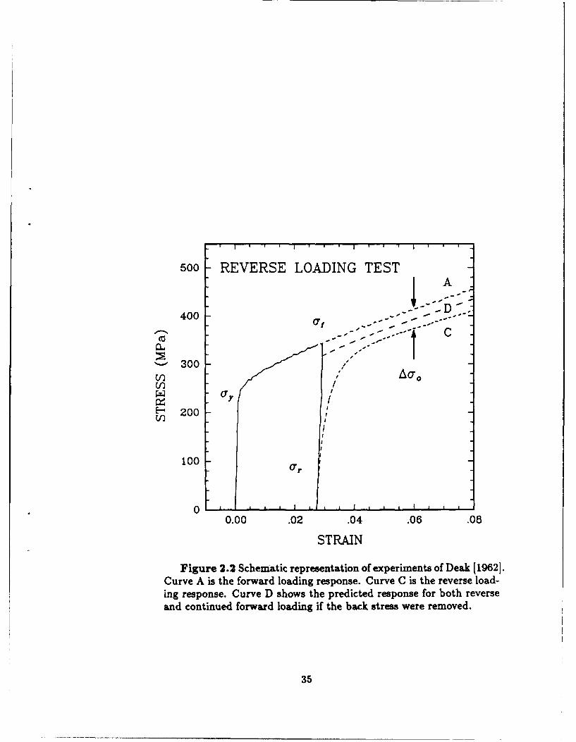
Figure 2.2 Schematic representation of experiments of Deak [19621.Curve A is the forward loading response. Curve C is the reverse load-ing response. Curve D shows the predicted response for both reverseand continued forward loading if the back stress were removed.

35

1600 Unannealed forware...,

1400-"

0 0, Unannealed reverse

800 Forward and reverse after annealing

-= 600

c2OO400

2001

5 10

Shear Strain (%)

Figure 2.3 Results of Deak [19621 for reverse and continued load-

ing of steel after annealing at 700'C for 1 hour. Unannealed forward

and reverse curves are shown for comparison.

36

(a)

1240 \ - "

01

irltr l 5ILS* |"

*0

I~as

151.100 002 004 a O0 010

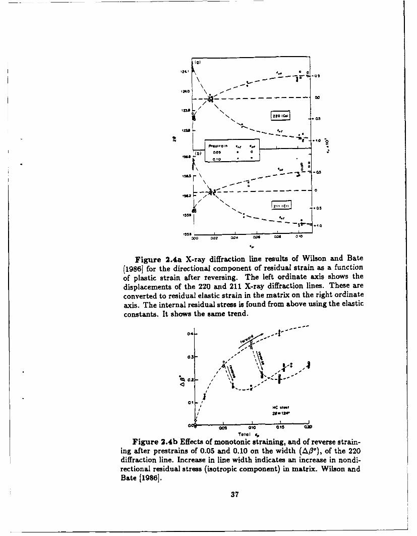
Figure 2.4a X-ray diffraction line results of Wilson and Bate(19861 for the directional component of residual strain as a functionof plastic strain after reversing. The left ordinate axis shows the

displacements of the 220 and 211 X-ray diffraction lines. These areconverted to residual elastic strain in the matrix on the right ordinateaxis. The internal residual stress is found from above using the elasticconstants. It shows the same trend.

04-

SI

0.2 -- ' '\ \ 44

} '

0.1 1

iI MC steel

o I I I

0 S 010 018

Total #

Figure 2.4b Effects of monotonic straining, and of reverse strain-ing after prestrains of 0.05 and 0.10 on the width (APO), of the 220diffraction line. Increase in line width indicates an increase in nondi-rectional residual stress (isotropic component) in matrix. Wilson andBate [19861.

37

10

(a) INTA LWN

1.0 0.5 10

50

10

(M PC) 150.

I I I253-0 2.5 2.0 1.5 1.0 0.5

4i.*

Figure 2.5 Results of Liu and Greenstreet [ 1976] for the backstress evolution during (a) forward and (b) reverse loading.In (h) the change in back stress from the forward loading value isplotted.

38

Tonsion V

.01 A

a Comnpressi On2

l00)

309

Chapter 3

Micromodeling of aParticle-Hardened Alloy Using theFinite Element Method

In modeling reverse plasticity the concept of a back 8tre8s or internal 8tress is widely

used to explain why yield occurs at a lower macroscopic stress in the reverse direc-

tion. It is postulated that straining in the forward direction induces a local residual

stress in the material. This residual stress acts to aid plastic flow in the reverse di-

rection. At least nominally, scientists would like to attribute the back stress variable

used in modeling with an actual residual stress in the material.

This is a difficult connection to make since the residual stress in the material

must be very local and thus difficult to measure. The material must contain a

residual stress distribution which equilibrates itself over a small size scale since the

manifestation of the back stress is still seen for a zero macroscopic stress. This

differs from the macroscopic residual stresses associated with, for instance, material

processing where the residual stress fluctuates over the length scale of the part.

The back stress is believed to result from the inhomogeneity of plastic Bow on

the microscale. A local system of internal stresses is set up which is manifested as

40

the back stress.

In this chapter, the development of a local residual stress field caused by the

interaction of an elastic particle with a surrounding elastic-plastic matrix is studied.

The residual stress stress-strain response of the system, particularly the observed

Bauschinger effect, is examined. This study is intended to model the deformation

of a particle hardened alloy.

The particle is modeled as purely elastic with the elastic constants for cementite

given by Laszelo and Nolle [19591: E = 29.042 x 10spsi, L = 0.361. The matrix

material is modeled as ferrite. It has both elastic and plastic strain hardening

properties. The elastic constants for ferrite were also taken from Laszelo and Nolle

[1959]: E = 30.174 x 10 6psi, v = 0.283. The yield and small-strain hardening

modulus were taken from Morrison [1966]. The modulus at strains greater than

25% was arbitrarily chosen low to give perfect or near perfect plasticity at large

strain. The actual input stress strain curves are shown in the next sections. The

matrix was modeled as hardening by classical isotropic hardening. This was chosen

to examine if the back stress could be developed by the particle-matrix interaction

and not by assuming kinematic hardening of the matrix. This is in accordance with

dislocation based models of the back stress.

Two finite element models were used in this study. The first uses an axisym-

metric unit cell to approximate a three dimensional array of spherical particles.

The second uses a plane strain unit cell modeling an array of cylindrical parti-

cles. The axisymmetric model gives a more realistic comparison with the actual

three-dimensional distribution of particles in a material. The plane strain model

has, however, the utility of allowing nonaxisymmetric loading such as simple shear.

41

This will be presented in detail below.

3.1 Axisymmetric Unit Cell Model

This model of the material system follows recent finite element studies of Tvergaard

[1982] and Needleman [1987]. Consider a material containing a periodic array of

elastic particles. This array is formed by stacking planes having particle spacings

shown in Figure 3.1a. The repeating unit in the plane is the hexagonal cell contain-

ing the particle at its center. In considering this boundary value problem we replace

the hexagonal unit cell boundary with a circular one. This is a close approximation.

If we now stack these cells so that the particles are directly above one another we

obtain the cylindrical geometry of Figure 3.1b. This represents an axisymmetric

column of particles. The most basic block that we can consider is one quarter of

the axisymmetric unit cell. This is illustrated in Figure 3.1c.

This region is divided into a finite element mesh which models both the particle

and the matrix. Figure 3.2 shows two meshes of this region. The mesh of Figure

3.2a contains 170 4-node axisymmetric elements (188 nodes). This is the basic

model used for this analysis. The total number of degrees-of-freedom for this model

is 330.

In order to verify whether this mesh is fine enough to capture the desired behav-

ior a second mesh (shown in Figure 3.2b) was used in some comparison calculations.

This second model has 600 elements (631 nodes) and 1180 degrees-of-freedom.

The boundary value problem that was solved with the axisymmetric model con-

sisted of various combinations of uniaxial tension and compression. Referring to

Figure 3.1b, the boundary conditions applied to each face were as follows: (f, rep-

42

resents the traction force in the i direction, and ui is the displacement in the i

direction)

" On the bottom face (Xs = 0)

f = 0

* On the left face (XI = 0)

U1 - 0

f= 0

" On the right face (XI = R)

fs= 0

ul constant. Where the constant is determined such that there is zero

radial force on the face, fo f, dy = 0.

" On the top face (Xs = b)

f = 0

U3 =constant. Where the constant vertical displacement was applied to

the entire face to simulate tensile or compressive loading.

Across the particle-matrix interface the displacements were continuous. The cell

had an equal radius and height, A. = B. in Figure 3.1b. The ratio of the particle

radius to the cell radius was 0.5759 . This gives an approximate particle volume

fraction of 12.7 %.

43

All simulations were conducted with the ABAQUS finite element code allowing

finite geometry changes. The code was run on a VAX 11-785 computer.

The total reaction force and displacement of the top face of the model were used

to derive the "macroscopic" true stress-true strain behavior of the system. They

were processed the same way that experimental load cell and extensometer signals

would be handled.

The input matrix plastic stress-strain curve is shown in Figure 3.3. The results

from Morrison [1966] only extended to about 25% strain so the matrix material was

assumed to be perfectly plastic above that.

Figure 3.4 shows the macroscopic stress-strain result for each of the two meshes.

The agreement is so close that the curves lie virtually on top of one another. Because

of this close agreement the more coarse mesh (Figure 3.2a) was determined to be

detailed enough for the present study. All of the following axisymmetric calculations

were conducted with this mesh.

In Figure 3.5 the uniaxial stress-strain curve is shown out to 15% strain. Notice

the gradual yield region and nearly linear hardening. This is compared in Figure 3.6

with the input hardening curve for just the matrix. This plot shows a comparison

of the flow stress of the system with and without the particles. The presence of the

elastic particles provides increased strain hardening as expected. Since the particles

only deform elastically the plastic strain is concentrated in the matrix. For a given

deformation, the matrix has then strain hardened more than it would have if the

particles were not present.

When the unit cell model is subjected to tensile straining followed by compressive

straining a stress-strain response exhibiting the Bauschinger effect is seen. An

44

example of this simulation is shown in Figure 3.7. Notice the gradual reyield in

compression.

In order to compactly compare the reversing results for a number of these pre-

strains the data is plotted in a standard way. For the reversing portions of the

curves only, the compressive region is shown but it is displayed in the first quadrant

by plotting the absolute value of stress against an accumulated strain where the to-

tal accumulated plastic strain is added to the elastic strain. This effectively rotates

the compressive stress-strain data by 180 ° about the zero stress point. Displaying

the data this way allows easy comparison of how the reverse yield has been lowered

and the extent of rounding during reverse flow. It also is convenient for displaying

the results of many tests.

In Figure 3.8 the simulations of six reversing tests are shown along with the

tensile loading curve. Each of the reversing curves exhibits the gradual reyield at

a lower stress magnitude than had occured during forward loading. The curves all

have a similar shape. The only difference between the features of these numerical

simulations and experiments is the absence of permanent softening. All of the simu-

lations go back to the forward loading flow stress level. It was extensively discussed

in Chapter 2 how real materials exhibit an isotropic softening during reverse flow.

The dislocations annhilate reducing the strength level. It is the isotropic softening

that gives the phenomenological feature of permanent softening. This finite ele-

ment model does not allow for isotropic softening. The matrix isotropic flow stress

is a monotonically increasing function of plastic strain. No mechanism has been

included to allow it to recover. This does not limit the model's ability to simulate

particle-matrix interaction during loading including back stress development. What

45

it does limit is the ability of the finite element model to correctly simulate isotropic

hardening after reverse plastic flow. This is not a severe limitation for our goal of

investigating back stress development.

One of the difficult determinations to make from a stress-strain curve like Figure

3.8 is what to use as the magnitude of the reverse yield in separating out the isotropic

and kinematic (back stress) portions of hardening.

The important issue is determining what position along the reverse loading curve

to use as the reverse yield point. This is difficult to resolve from just a stress-strain

curve due to the smooth reyielding behavior during reverse loading. If the reverse

yield point is known then the one dimensional elastic region is known and the shift

of the yield surface during the initial straining is known. The hardening during

forward loading can then be separated into isotropic and kinematic components

(neglecting yield surface distortion).

The back stress determined from the stress strain curve should have a physical

connection with the residual stress left in the material after forward loading. In

order to explore this connection, the stress distribution in the finite element model

after prestraining and unloading to zero macroscopic stress was examined. An

example of the residual stress component in the direction of prestraining is shown

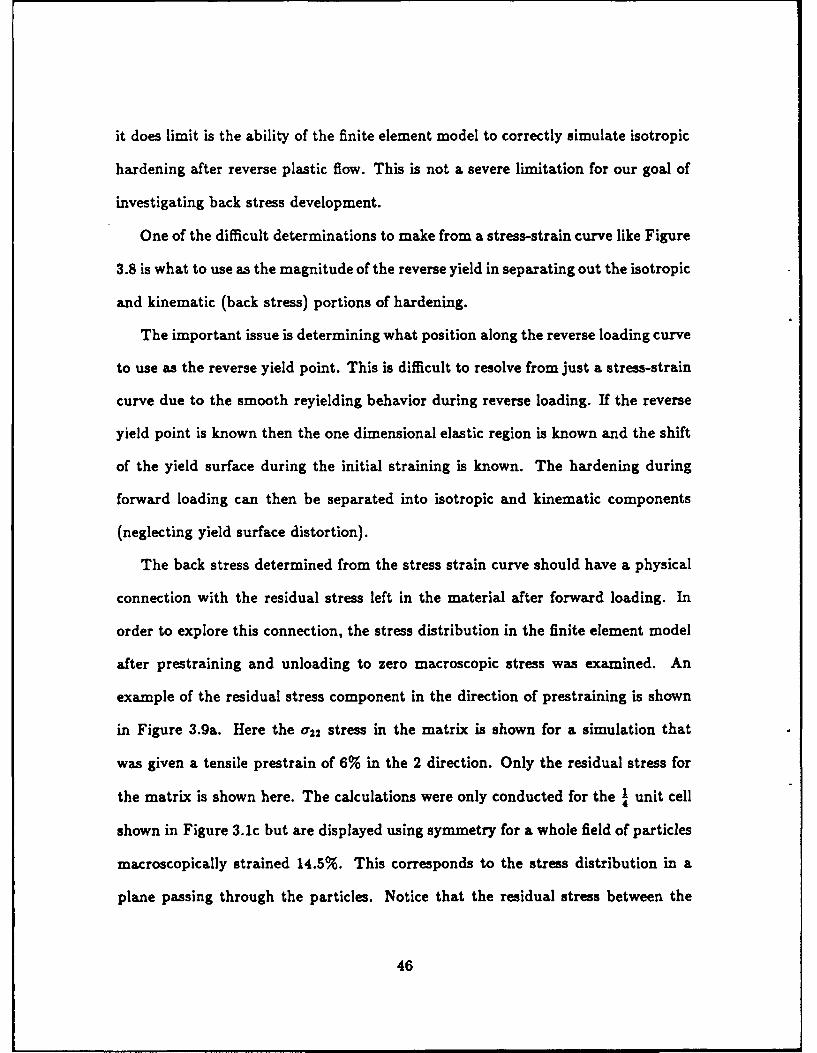
in Figure 3.9a. Here the a22 stress in the matrix is shown for a simulation that

was given a tensile prestrain of 6% in the 2 direction. Only the residual stress for

the matrix is shown here. The calculations were only conducted for the 1 unit cell4

shown in Figure 3.1c but are displayed using symmetry for a whole field of particles

macroscopically strained 14.5%. This corresponds to the stress distribution in a

plane passing through the particles. Notice that the residual stress between the

46

particles in the direction of loading is tensile while the residual stress in the rest

is compressive. Equilibrium requires there be both tensile and compressive stress

which balance out over the whole cell.

The distribution of the residual stress lends insight into the mechanism of the

Bauschinger effect. The system can be viewed as columns of one type of material

(the stacking columns of the particles with the matrix separating them) contained

in an annulus of another material (purely matrix). When the system is strained the

annulus develops a greater averaged plastic strain (the particles can contain larger

elastic strains). Once the extenal force is released, the annulus holds the particles

apart creating tensile residual stress between them. The system is analogous to two

springs which have been strained different amounts. One is placed in tension and the

other in compression. This is the type of phenomena that the mechanical 8ublayer

model was constructed to model. For the particle-matrix unit cell loaded along

the particle row direction we can think of a sublayer model having two elements.

Unlike that model there is extensive interaction between the two elements since

neither deforms homogeneously. Here we clearly see that there is an internal stress

field because of the inhomogeneous deformation of the system.

The accumulated equivalent plastic strain distribution is shown in Figure 3.9b.

The macroscopic plastic strain in the direction of straining for the cell was 0.0598.

This distribution shows that the strain is concentrated above the particle but the

gradation is quite gradual except near the particle-matrix interface.

In a physical experiment there can be slight nonuniformity of deformation in

the gauge region due to specimen geometry or loading alignment. This can cause

the proportional limit of the stress-strain curve to differ somewhat from the point

47

where plastic flow first occurs throughout the specimen. This is not the case in our

numerical experiment. Plastic flow initiates nonuniformly within the unit cell but

is representative of yield occuring simultaneously in all of the repeating cells.

By taking the proportional limit as the reverse yield for the numerical stress-

strain curves we can determine the back stress as the center of that elastic region.

This back stress value correlates well with the residual stress distribution (at zero

macroscopic load) in the matrix. The tensile back stress determined from the stress-

strain result for the prestraining of 14.5% shown in Figure 3.10 was 21,000 psi. If we

tried to select one number from the residual stress field of Figure 3.9c as representing

its average then 21,000 psi would be reasonable.

This demonstrates a correspondance between the back stress determined from

a small strain offset yield definition (in the numerical case an offset of zero) and

the actual residual stress in the material system. It is important to have this

connection. Otherwise the back stress is just a modeling variable not in touch with

reality. A physical correspondance is needed when examining deformations having

material rotation. We need to properly model the back stress for this region. In

the literature, this has not been carried out.

Using the proportional limit definition of reverse yield, the results of Figure

3.8 were separated into isotropic and back stress components. The summary of

this separation is shown in Figure 3.10 . Notice how the back stress initially rises

quickly but has nearly saturated by 6% plastic strain. The isotropic part continues

to rise nearly linearly with plastic strain throughout this region. These results are

in agreement with experimental observations.

This result shows how the back stress increases with plastic strain for forward

48

straining from the virgin condition. We are also interested in how the back stress

evolves during reverse plastic flow. To look at that, the model was prestrained

in tension to about 6%. It was then reversed to a certain strain. Finally, it was

again pulled in tension. This was done for 5 different amounts of reverse strain-

ing. By plotting the position of the center of the elastic region determined from

the reloading branches, the evolution of the back stress during reversing could be

traced. The reversing and reloading branches are all shown together in Figure 3.11

. Each reloading branch represents a separate test. The back stress evolution from

this is shown in Figure 3.12. The tensile back stress value is plotted against the

accumulated strain during the reversing branch. The initial back stress value was

17.3 ksi. During reversing it rapidly decreases to zero and tends toward the value it

had prior to reversing. The back stress rapidly changes sign and becomes negative

during this reverse flow. This is in close agreement with the results of Wilson and

Bate [1986]. Compare Figure 3.12 with Figure 2.4. They also show this same trend

from their x-ray measurements.

This same behavior is seen by Liu and Greenstreet [1976] who plotted yield

surfaces during reverse flow and took their centers as the back stress. The same

rapid decrease, change of sign and gradual increase in magnitude of the back stress

was also noted in their work.

In Figure 3.11, The final, tensile loading branch crosses the prestress point at a

higher stress value. For small enough hysteresis loops this is not seen experimentally

but rather the reloading undershoots, slightly, the prestress point. This also is a

result of the isotropic softening that takes place in the material but is not modeled

with this calculation.

49

The final simulation with the axisymmetric unit cell model involves a fixed

strain amplitude, cyclic test. The cell was cycled through 5 cycles of ±2% strain

cycling. The stress-strain results are displayed in Figure 3.13. Even after 5 cycles

the response is toward a stable, symmetric, saturated, hysteresis loop. This shape

is typical of experimental results also. The saturation is achieved and the flow

strength is limited because the input flow stress for the matrix material saturates

at 100 ksi.

From this axisymmetric model many of the uniaxial, experimental results can

be qualitatively reproduced. The back stress evolution both in forward and reverse

flow is correctly simulated. The back stress is shown to roughly correspond to the

residual stress in the matrix annulus surrounding the particles. The experimental

feature that is not reproduced by the numerical model is permanent softening.

If the ideas of Chapter 2 are appropriate then this is not a suprise. Permanent

softening results from the reduction of the isotropic component during reversing.

Since classical isotropic hardening was used for the matrix material then this is not

possible with the current model.

3.2 Plane Strain Unit Cell Model

The axisymmetric model is only useful for axisymmetric loading geometries, having

symmetry about the same axis. For the important case of simple shear, the bound-

ary conditions are nonsymmetric. In order to model particle-matrix interaction

with a two dimensional mesh geometry we consider a plane strain analysis.

Considering the mesh shown in Figure 3.14, the particle is modeled as a cylinder

whose axis is perpendicular to the plane of the paper. The matrix surrounds the

50

particle as before. Notice that the full unit cell is modeled and not just one quarter

of it as was done with the axisymmetric model. The elastic properties are identical

to those used for the axisymmetric model but the matrix flow stress level is slightly

different. The stress-plastic strain curve input for the matrix is identical to Figure

3.3 up to a plastic strain of 25% but then instead of being perfectly plastic above

that it continues to harden at a reduced modulus up to a plastic strain of 500% (see

Figure 3.15). Above this the model is perfectly plastic. The reason for continuing

hardening to larger strains is that the plane strain model was to be used to larger

strains.

The mesh contains approximately the same level of detail as the axisymmetric

model. It has 711 nodes, 720 elements and 1403 degrees-of-freedom. The four outer

surfaces of the mesh are all constrained to remain in straight lines. The ratio of the

diameter of the particle to the cell width is 0.402 . That gives a particle volume

fraction of 12.7% which is the same as for the axisymmetric model although the

particle geometry is different.

3.2.1 Tensile Loading

In order to get baseline results for comparison, the model was first loaded to simulate

tensile loading. The bottom edge of the model was restrained against vertical

motion. The left and right sides were forced to remain straight and vertical with

zero horizontal force. The top edge was displaced vertically to simulate tensile

straining. Referring to Figure 3.14, the boundary conditions applied to each face

were as follows: (fi represents the traction force in the i direction, and ui is the

displacement in the i direction)

* On the bottom face (X2 = 0)

51

u2 =0

f,= 0

e On the left face (X, = 0)

f2 =0

* On the right face (Xi = L)

f2 = 0

ul = constant. Where the constant is determined such that there is zero

horizontal force on the face, F, = 0.

* On the top face (X2 = L)

fi = 0

U2 =constant. Where the constant vertical displacement was applied to

the entire face to simulate tensile loading.

In Figure 3.16 the macroscopic stress-strain result for the model is shown up

to a macroscopic true strain of just over 40%. The deformed mesh at this level

of deformation is also displayed in Figure 3.16a. This represents the upper limit

to which this mesh can be pushed without the need to remesh due to distortion.

Notice the decrease of the hardening modulus. The nearly linear hardening region

observed for the macroscopic result of the axisymmetric model (Figure 3.4) is also

observed here for strains below 10%. Between 10 and 20% strain the macroscopic

result shows a transition to a lower hardening modulus. This corresponds to a large

52

portion of the matrix hardening to beyond the knee of the input stress-strain curve

(local strain of 25% in Figure 3.15). The macroscopic result follows the matrix

hardening behavior.

3.2.2 Simple Shear

In order to simulate the simple shear deformation mode, new boundary conditions

are applied to the plane strain model which has been described above. The main

idea is to hold the bottom edge of the model fixed and to horizontally displace the

top face. Referring to Figure 3.14, the boundary conditions applied to each face

were as follows: (f, represents the traction force in the i direction, and ui is the

displacement in the i direction)

* On the bottom face (X 2 = 0)

U 1 =0

U 2 = 0

a On the left face (XI = 0)

ul and U2 enforced to remain on a line connecting the top left and bottom

left corner nodes.

# On the right face (XI = L)

ul and u2 enforced to remain on a line connecting the top right and

bottom right corner nodes.

e On the top face (X 2 = L)

U2= 0

53

ul =constant. Where the constant horizonal displacement was applied

to the entire face to simulate simple shear.

During large strain simple shear, not only does a shear force develop but a

normal force is also required to keep the shearing faces held at a constant distance

apart. By measuring the reaction forces on the top row of nodes required to enforce

the above displacements we derive the macroscopic stress response shown in Figure

4.17. In Figure 4.17 we also see the deformed mesh at a shear strain of -Y = 0.5.

The corresponding stress-strain response is shown in Figure 3.17b. The axial stress

shown in the plot is the 022 component on the top face. As the model deforms it

develops a compressive, vertical, normal stress. This is in qualitative agreement with

the experimental literature [Montheillet, Cohen and Jonas, 1984]. If no particles

were present then the predicted normal stress would be approximately -158 MPa.

This is insignificant when compared with the result of -2148 MPa predicted here

with the particle. The shear stress behavior shown here is in agreement with the

shape of the plane strain tension result of Figure 3.16. Here we see that the finite

element model is able to qualitatively give the correct behavior for large strain

simple shear.

Micromodeling using finite elements shows great promise for understanding the

deformation behavior of particle hardened alloys. The interaction between the dif-

ferent phases can be properly taken into account and give qualitatively correct

results for the macroscopic behavior of Bauschinger effect and large shear tests.

54

(a) (b)

~X3I

0R

0 -1

0A

(c)

Figure 3.1 Modeling of a doubly periodic array of spherical, elas-tic particles in an elastic-plastic matrix, a) Hexagonal cell boundariesare approximated as circles. b) The cylindrical columns can be mod-eled using 1 of the unit axisymmetric cell. c) The finite element4discretization of the basic region.

55

(a)

(b)

Figure 3.2 Two finite element discretizations of the axisyxnmetriccell. a) Mesh used for axisymrnetric calculations. It contains 170

elements. b) Finer mesh used for convergence comparison. It contains600 elements.

56

X10 5

1.25

S" 8.75

Cl)

8.25

6.88 8.05 0.18 8.15 0.20 0.25

Strain

Figure 3.3 Input stress-plastic strain curve for matrix material,from Morrison [1966].

57

88888

m 48888--

28888--

8.88 8.81 8.8 8.83 8.04 8.8s 8.86

Strain

Figure 3.4 Comparison of macroecopic stress-strain result for unitcell pulled in tension using both the coarse mesh and the fine mesh ofFigure 3.2.

58

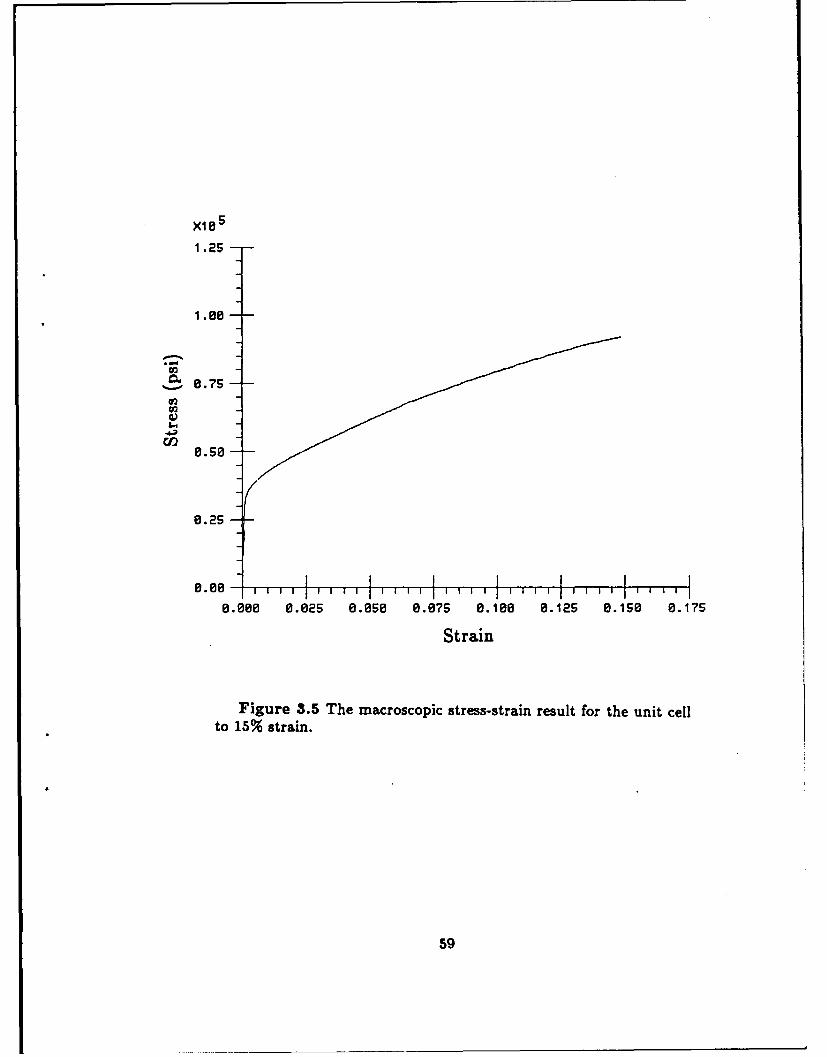
X10 5

1.25

8.75-

0.50

0.25

0.000 0.025 0.050 0.075 0.100 0.125 0.150 0.175

Strain

Figure 3.5 The macroscopic stress-strain result for the unit cellto 15% strain.

59

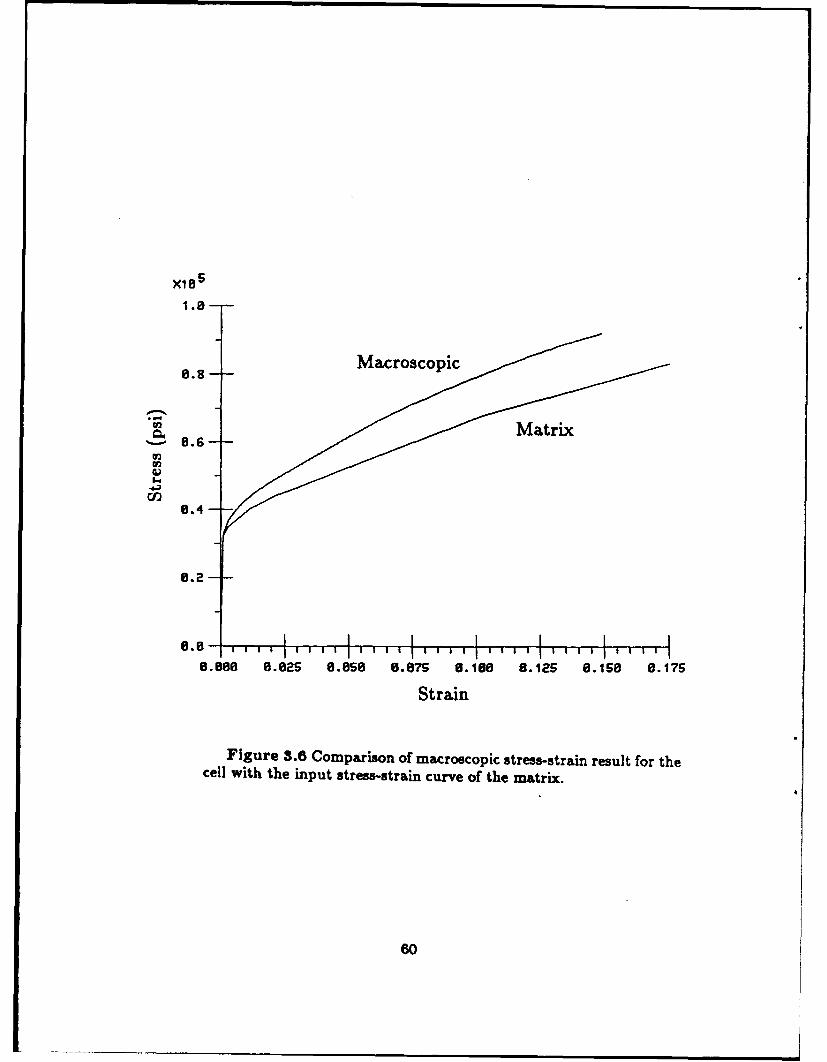
X18

e.8 Macroscopic

0.6-

8.4-

0.2-

8.0 8.825 8.856 8.875 8.188 8.125 8.158 8.175

Strain

Figure 3.6 Comparison of macroscopic stress-strain result for thecell with the input stress-strain curve of the matrix.

60

X10

1.08

8.5-

CI

-8.83 -0.82 -0.81 0.88 0.81 8.82 8.83

Strain

Figure 3.7 Example of the response of the cell for loading in ten-sion followed by loading in compression.

61

X105

1.25

1.00

.-

0 .75

0.25

0.00 I -T- I I I I I I I

0.00 6.05 0.10 0.15 0.20

Strain

Figure 3.8 The reversing branches of 6 numerical simulations oftension-compression applied to the unit cell. The compressive resultsare rotated into the first quadrant for compactness.

62

(a)

9/

8 ~ 6

Contour Stress 10, 85

(k":D 7

1 -50 II

2 -403 -304 -205 -10

6 07 +10

8 +209 +30 4

10 +4011 +50 3

(b)

Contour Plastic 7 U

Strain 3

1 02 0.0253 0.0504 0.0755 0.1006 0.1257 0.1508 0.175

5

Figure 3.9 Contours for residual state in cell obtained by uni-

axial loading to Z = 6% followed by unloading to zero external load.

a) Contours of residual vertical, normal stress 022. b) Contours of

accumulated equivalent plastic strain.

63

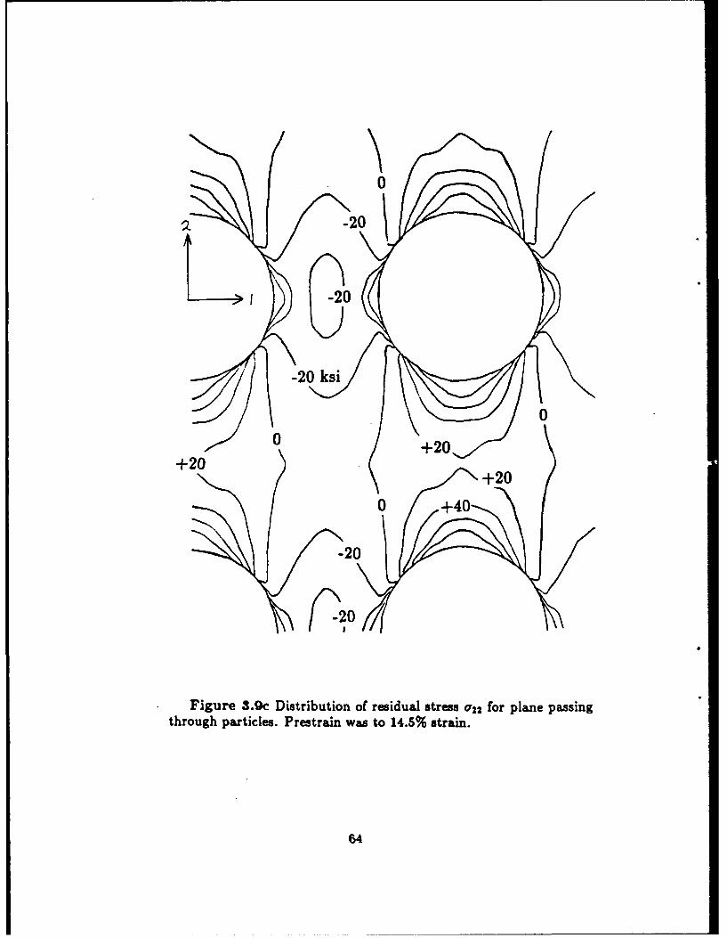
00

-20 ks

000 ] 20j

+20

Figure 3.9c Distribution of residual stress a22 for plane passingthrough particles. Prestrain was to 14.5% strain.

64

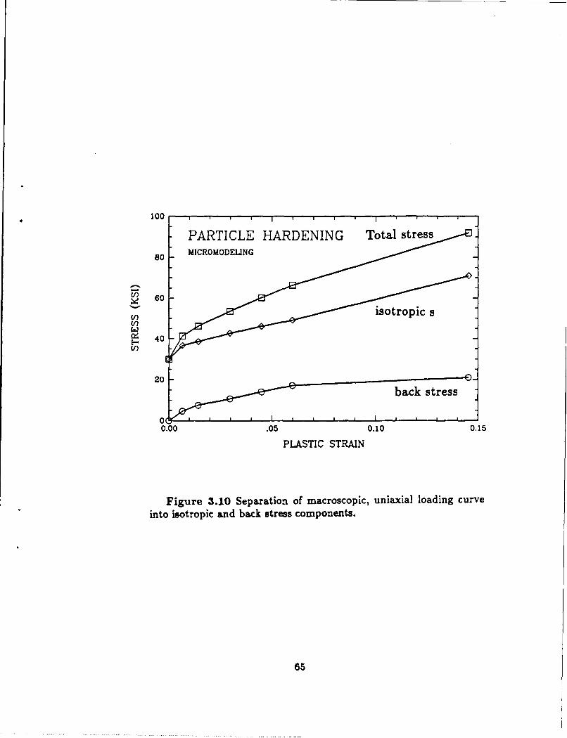
PARTICLE HARDENING Total stres6 MICROMODELNG

10-

EE

60..

S40

V2

-back

stress

0.00 .05 0.10 0.15

PLASTIC STRAIN

Figure 3.10 Separation of macroscopic, uniaxial loading curve

into isotropic and back stress components.

65

X10 5

1.0--

06E

4f)

0.00 0.01 0.02 0.03 0.04 0.05 0.06 0.07

Strain

Figure 3.11 Macroscopic stress-strain results for forward loadingfollowed by different amounts of reverse strain which is then followedby forward loading. Five different reloading branches are shown.

66

I i I I I mI P

20PARTICLE HARDENINGREVERSE FLOW BEHAVIOR

10

-oV)

-10z

- 15

0.00 0.10 0.20 0.30 0.40 0.50 0.60 0.70 0.80 0.90

Accumulated Strain (M)

Figure 3.12 Evolution of the back stress with accumulated straindetermined from the simulations of Figure 3.11.

67

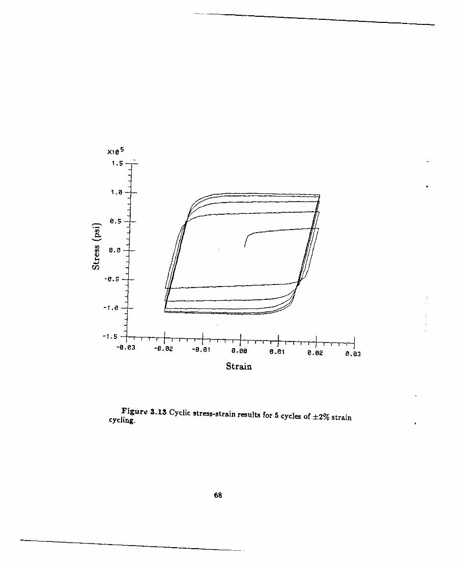
X1.5

1.5

L4

Cl)

-0..3 -0.02 -0.01 e.00 0.01 8.02 8.83

Strain

Figure 3.13 Cyclic stress-strain results for 5 cycles of ±2% straincycling.

68

Figure 3.14 Finite element mesh used for unit cell of plane strainmodel.

69

X105

1.25

1.00t

8.75

,d

1 0.58 -

8.25

0.00-

8.00 8.25 8.58 0.75 1.00 1.25 1.50

Strain

Figure 3.15 Input stress-strain curve used for modeling the ma-trix material for the plane strain simulation.

70

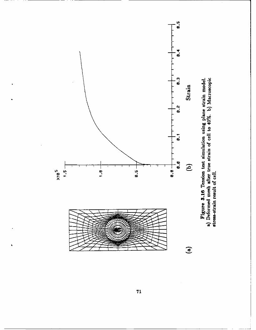
Lh

CDu

71.

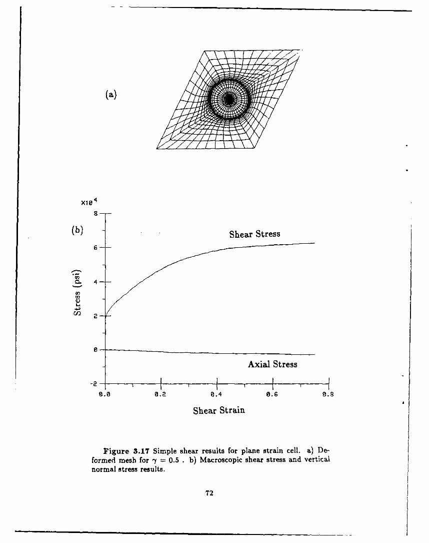
(a)

(b) Shear Stress

6--

~4 -4

I' 2-

Axial Stress

-2 1

0.0 6.2 0.4 0.6 0.8

Shear Strain

Figure 3.17 Simple shear results for plane strain cell. a) De-formed mesh for -y = 0.5 . b) Macroscopic shear stress and verticalnormal stress results.

72

Chapter 4

Review of Plasticity Modeling

In this chapter the relevant, published work is surveyed to guide constitutive mod-

eling. This work is reviewed with the goal of extracting the important behavior to

be modeled as well as the sufficiency of the current constitutive models to predict

this behavior.

First, the experimental literature is briefly reviewed to identify the important

behavior. The prominent areas of experimental research in metal plasticity investi-

gated are: large strain experiments (primarily unidirectional), and cyclic plasticity

(many stress reversals, both proportional and noiiproportional).

In order to develop a model which can unite these classes of behavior the consti-

tutive models particular to each of these classes were also summarized: large strain

and cyclic modeling. From this review we will be able to identify several phenom-

ena which have not been previously modeled but which lend great insight into the

material behavior.

73

4.1 Experimental Review

4.1.1 Large Strain

Experimental studies of metals deformed to large strain have been conducted ex-

tensively over the last century. Different testing modes and test techniques have

been developed and used with varying degrees of success. In this section only major

trends and behavior are summarized. A more detailed discussion of large strain,

experimental plasticity is presented in Appendix A.

The following list displays some of the important observed material behavior:

1. Initial yield and strain hardening are generally the same as observed in small

strain experiments.

2. Strain hardening continues to many hundred percent strain. This is unlike

elevated temperature testing which shows a stress saturation.

3. The equivalent stress during plastic flow is deformation mode dependent. For

the same equivalent strain, torsional deformation occurs at a lower equivalent

stress than tensile or compressive deformation.

4. For torsional deformation substantial axial, normal stress is developed at large

strain when the specimen is restrained from axial displacement. If the speci-

men is unrestrained in the axial direction then axial strain accumulates with

plastic deformation (the Swift effect).

This list is quite short because, even though there have been many large strain

experiments, they have generally been restricted to one dimensional, monotonic

loading. A useful model also needs to be able to adequately predict and represent

74

multiaxial, nonmonotonic loading conditions. To better understand the material

response in these regimes we examine the cyclic plasticity literature as a guide to

complex material response.

4.1.2 Cyclic Plasticity

Cyclic material response can vary quite markedly from pure monotonic behavior.

Often the cyclic behavior of a metal is represented by a single cyclic stress-strain

curve formed by connecting the tips of saturated hysteresis loops of various widths.

Of course, this information alone does not properly represent all of the possible

cyclic responses. There is a rich variety of phenomena for the many different types

of cyclic loading. The cyclic results in the literature are limited to small strain.

This section will present some of the important behavior from the literature and

draws largely from several review-type papers: Dolan [1965], Drucker and Palgen

[1981], Dafalias [1984b], and Chaboche [1986]. First, behavior from uniaxial, cyclic

tests will be discussed. This will be followed by results of multiaxial, nonpropor-

tional loading tests.

The most fundamental cyclic test in one in which the specimen is uniaxially

cycled between constant strain limits centered on zero strain. The material will

either show progressive hardening with each cycle or progressive softening depending

upon the prior history of the material. Generally, an annealed material will harden

and a cold-worked material will soften. Eventually the material responds with a

saturated hysteresis loop, symmetric about the -tress axis, that does not change with

increasing numbers of cycles. For most materials, this steady state loop depends

much more strongly upon the magnitude of the cyclic strain then it does upon the

75

prior strain history [Morrow and Tuler, 1965].

If a specimen is cycled between two strain limits which are not centered on zero

then the first cycle will show a nonzero mean stress (mean of the maximum and

minimum stress in the cycle). As cycling continues, the specimen will relax as the

mean stress tends toward zero and a stable, symmetric hysteresis loop is formed.

Again the cyclic strain range being most important in the size of the stress range.

The cycle shows mean 8tress relaxation.

A specimen that is cycled between stress limits not centered on zero stress will

show cyclic creep. With each cycle a small mean plastic strain will accumulate in the

direction of mean stress. For many cycles this can give a substantial accumulation

of plastic strain.

An example of this cyclic creep was given by Feltner [1963] for near pure alu-

minum. He measured the cyclic creep and compared that with the dislocation cell

structure developed after various numbers of cycles. A very interesting result was

that the dislocation density and cell structure was essentially unchanged from the

first half cycle to more than 3400 cycles when a creep strain of more than 30 % had

accumulated, see Figure 4.1. This is very different from monotonic loading where

the dislocation density monotonically increases with plastic strain. Feltner cited

two possible explanations for this behavior. The first would be that during a cycle

few dislocations are generated but the existing ones move relatively long distances.

The second explanation would be that during a cycle many new dislocations are

created, move a short distance, and are annhilated. For the constancy of disloca-

tion loop density that was observed there would have to be a balance between the

dislocations that are created and those that are annhilated during each cycle.

76

Since the dislocation loop density is largely unchanged over many cycles, the dif-

ference between monotonic and cyclic behavior is substantiated on the microscopic

as well as macroscopic scale. Cyclic behavior does not show the dramatic structural

changes seen in monotonic loading.

In a recent paper Trampczynski [1988] conducted back stress evolution studies

on two steels using a partial, successive unloading technique. He used a 0.05%

offset definition for reverse yield. His results reinforce many of the observations

made above:

* The general shape of the back stress path is established during the first loop

of cyclic loading and changes only slightly for further cycles.

* The cyclically stable maximum values of back stress and isotropic component

depend upon plastic strain amplitude.

* After prestrain in one direction, cyclic loading causes the isotropic component

to soften.

The experimental results for nonproportional cyclic straining contain even

more material phenomena which lend insight as well as require modeling. A sum-

mary of the most important differences of nonproportional cycling compared to

proportional is presented below.

In 1978, Lamba and Sidebottom [1978a] conducted multiaxial experiments an

tubular specimens of OFHC copper. They first recognized the main features of

multiaxial, cyclic plasticity. The results for stable, hysteresis loops cycled between

symmetric strain limits showed that there is one cyclic stress-strain curve for pro-

portional loading whether conducted in tension/compression, torsion, or in-phase

77

tension/torsion. Plotting the maximum Mises equivalent stress against the max-

imum equivalent plastic strain range gave one curve independent of the loading

direction as long as that direction remained constant throughout the test.

A dramatic result was seen when the combined tension/torsion straining was

changed so that it was no longer proportional but 900 out-of-phase. This type of

loading consists of cycling the axial strain and the shear strain where one lags the

other by 900. The material showed continued hardening above that for a uniaxial

test. It formed a stable hysteresis loop at a stress level 40 % higher than that at

the same maximum plastic strain range in the proportional (or in-phase) test. This

level was independent of whether the specimen was initially cycled uniaxially or

not.

This additional hardening due to out-of-phase straining has been noted more re-

cently by other researchers also conducting tests of this type. Kanazawa, Miller and

Brown [19791 have noted it in a 1% Cr-Mo-V steel. Krempl and Lu [1984] observed

it type 304 stainless steel at room temperature. Cailletaud, Kaczmarek and Poli-

cella [1984], and Benallel and Marquis [1987] have studied the additional hardening

in 316 stainless steel. The amount of additional hardening is strongly influenced

by the degree of nonproportionality in the loading. The maximum hardening is

seen for a 90 out-of-phase test where, for instance, a sinusoidal input is given to

the axial and torsional strain controllers with the torsional signal lagging the axial

one by 90 ' . The stress response for such a test is shown in Figure 4.2. Notice the

hardening to a saturation stress magnitude. The final, multiaxial hysteresis loop is

symmetric about the stress origin.

Additional hardening is seen, not only for out-of-phase cycling but for any change

78

in cycling direction. Benallel and Marquis [19871 note increased stress levels when

changing from tension-compression to torsional cycling.

A final observation for multiaxial, cyclic loading concerns the loss of the addi-

tional strength when uniaxial cycling is resumed. A specimen that has saturated

at the higher stress level due to out-of-phase cycling will soften if uniaxial cycling

is added having the same maximum strain range. The additional hardening fades

slowly with the cycling. This was observed by Lamba and Sidebottom [1978a] (they

noticed that the additional hardening could be erased ) and Cailletaud, Kaczmarek

and Policella [19841.

Trampczynski [19881 also observed that additional hardening is caused by the

isotropic component. Resuming uniaxial cycling causes the isotropic component to

soften back to the unique value associated with that strain amplitude.

Lu [19861 presented data for 900 out-of-phase stress cycling of 6061-T6 aluminum

alloy. Unlike with strain controlled cycling here strain is the response to the stress

input. The stress rate is always perpendicular to the stress direction. Lu's results

showed that the plastic strain rate does not have the same direction as stress for

this loading. It bends toward the loading direction.

Several authors have also presented data for general, nonproportional loading

blocks. It is not clear what specific phenomena can be cited from these tests but they

do provide data to be used for general evaluation of cyclic models. These results are

in [Lamba and Sidebottom, 1978b], [Cailletaud et al., 1984] and [McDowell, 1985].

79

4.2 Review of Constitutive Modeling

The previous section contained a description of the important material behavior to

be modeled. This section examines the current constitutive modeling ideas in light

of these phenomena.

A review of plasticity's early beginnings is not included here since that infor-

mation is readily available elsewhere [Hiil, 1950]. The constitutive model that has

proven most useful for small strain plasticity is commonly referred to as the Prandtl-

Reuss equations.

dT' 3 dO'T12G+ 2crH

dci 3d ar.K

where a is the equivalent stress (o = {IT' -Tl'}), H is the slope of the equivalent

stress-plastic strain curve, K is the bulk modulus and G is the elastic shear modulus.

This is the plasticity theory most commonly found in computer codes today.

The other most significant small strain theory is due to Prager [1956] with

modification due to Ziegler [1959]. This is referred to as kinematic hardening. The

yield surface does not expand in stress space but rather translates. The translation

of the yield surface center, B, is given by

dB = Cdi? ,

where C is a scalar.

4.2.1 Large Strain Extensions of Previous Theories

The extension of constitutive theories valid for small amounts of deformation to

ones suitable to describe finite deformation is not a straightforward process. Both

80

the kinematics of large deformation and the issues of material objectivity need to

be addressed.

Around 1970 Budiansky [19701 proposed an extension of the Prandtl-Reuss equa-

tions in which he used the Cauchy stress measure with the kinematics defined in

terms of the curvilinear coordinates. This theory was used by Needleman [1972]

to study the growth of voids. Hutchinson [1973] modified the theory by replacing

tne Cauchy stress with the Kirchhoff stress. This involved very little change to the

theory for metals where the bulk modulus is much greater than the applied stress

level. The benefit of this replacement is that it makes the finite element implemen-

tation easier since it leads to a symmetric formulation. Hibbitt, Marcal and Rice

[1970] and also McMeeking and Rice [1975] were involved in concurrent extensions

of the small strain Prandtl-Reuss equations.

Analogous to the way that the isotropically hardening theories developed in

the small strain regime the large strain version of kinematic hardening was pro-

posed in 1978 by Tvergaard [1978]. He used this theory to analyze biaxial necking.

Calculations of bifurcation loads and strain levels have always been overestimated

by models based on purely isotropic hardening. Tvergaard found that the softer

transverse response of kinematic hardening better predicted the stress levels of local-

ization but stiji overestimated the strains where localization occurred. Tvergaard,'s

model generalized the Prager-Ziegler evolutior law for the bac.k stress by replacing

the material time derivative with the Jaumann derivative.

B = B-WB + BW = -B)

where B is the back stress, W is the spin (= skew part of the velocity gradient ), r

is the Kirchhoff stress (=Tt), T is the Cauchy stress.

81

This substitution seemed natural from the mathematical viewpoint of formalism

required to make the equation objective.

The formulation of a model which combines the features of isotropic and kine-

matic hardening was proposed by Key, Biffle and Krieg [1977] and used to calculate

metal forming processes by Key, Krieg and Bathe [1979]. Since material data is not

generally available in the literature to partition the hardening into realistic percent-

ages of kinematic and isotropic components they chose to model their material as

purely kinematically hardening.

The extension of the notion of kinematic hardening from small strain to large

strain by the substitution of the objective Jaumann stress rate for the material stress

rate in the equations of Prager-Ziegler was severely challenged in a presentation at

a workshop held at Stanford University in 1981 by Nagtegaal and deJong [1982].

They showed that if this extension is used, then if the material is sabjected to simple

shear, such as in the fixed end torsion test, stress oscillations are predicted for both

the shear and normal stresses. This response was unexpected for a monotonic

loading condition.

This result sparked much interest in finite strain constitutive modeling. Simple

shear is unlike many of the loading conditons that had been considered for model

verification. The tensor stretching component is equal in magnitude to the con-

tinuum spin (skew symmetric portion of the velocity gradient). Lee, Mallett and

Wertheimer [19831 explained that use of the Jaumann derivative in the back stress

evolution equation leads to a back stress ,ensor that continues to rotate in stress

space even though the deformation is bounded. They proposed using the spin of

a material line element that instantaneously coincides with direction of the eigen-

82

vector corresponding to the largest back stress eigenvalue in a corotational stress

rate.

BL= B - WLB + BWL,

where WL is the spin of the material line coincident with the direction of the largest

eigenvalue of the back stress.

This choice of stress rate does remove the oscillations for a sufficiently large

hardening modulus but does not produce a monotonic shear stress response if the

hardening modulus is low or, especially, if the hardening modulus decreases with

strain (Reed and Atluri [19851).

A number of different choices for the spin to be used in a corotational type rate

have been proposed. Among them are the Green-Naghdi rate proposed by Dienes

[1979,1986] and Johnson and Bamman [1984] and the "elastic" or "accomodating"

spin of Dafaiias [1984c], Loret [1983], and Anand [1985].

The use of tensor representation theorems to construct constitutive relations

for the total velocity gradient, not just the symmetric part, has been pursued by

Dafalias [1984c], Loret [1983], and Anand [1985]. Lee [1969] had proposed decom-

posing the deformation gradient, F, into elastic and plastic parts,

F = F'FP.

Dafalias, Loret and Anand have taken the approach that FP is defined in an analo-

gous way to one dimensional, small plastic strain. Consider unloading the body that

has been deformed, then orienting the material elements, with respect to a spatial

reference frame, to the identical orientation they had in the original configuration.

The FP is then just that transformation which takes the original configuration to

this specially oriented, relaxed configuration.

83

This is not the only way to prescribe the partitioning of the F'FP decomposition.

Fardshisheh a-d Onat [1974] and Parks et. al. [19851 require that F' be a pure

straining such that F' = F T. They embed the plastic spin in a skew symmetric ex-

pression which is prescribed without additional constitutive modeling. Loret [1983]

and Dafalias [1984c] presented the general forms for representing a skew symmetric

tensor such as spin by using the representation theorems of C.C. Wang [1970]. By

using the lowest order generator which is derivable from two symmetric tensors they

propose a constitutive law containing one scalar material function. Loret [1983] and

Dafalias [1984a, 1984c, 1985] examine the response of this type of model for simple

shear. They show that for proper choice of the scalar parameter the stress oscil-

lations predicted by the kinematic hardening model can be removed. Also they

showed that the magnitude of the normal stress which develops during large simple

shearing can be controlled by this parameter. Without attempting to match exper-

iments they have demonstrated that including plastic spin in the material model

provides better qualitative predictions.

Dafalias has also applied the inclusion of plastic spin into an illustration of

a transversely isotropic material (Dafalias [1984c]). Here the significant material

directions can be more easily visualized than with kinematic hardening.

Anand [19851 applied a full state variable representation to finite, elastovis-

coplasticity. He shows the construction of a phenomenological theory, the form of

which follows from the use of Wang's tensor representation theorems. By proper

simplification the traditional plastic stretching flow rule is recovered. This form is

equivalent to that proposed by Dafalias and Loret for rate-independent plasticity.

Paulun and Pecherski [1985,1987] argue for a particular choice of the constitutive

84

function for the plastic spin. Their choice is equivalent to the spin of the material

line element initially perpendicular to the shear direction. This selection also gives

monotonic behavior in simple shear.

In reviewing this flurry of stress rate proposals, Reed and Atluri [1985] reexamine

the simple shear results of classical (Jaumann rate) kinematic hardening, that of the

"Green-Mclnnis" rate presented by Dienes [1986], and the rate of Lee et al. [1983].

They point out that none of these stress rates predict normal stresses having the

proper order of magnitude for the limited torsion results from the literature. This

author would like to point out that no material has been shown to harden entirely

by kinematic translation of the yield surface either. Reed and Atluri correctly assert

that the discrepancy in stress rates can be absorbed on the right hand side of the

equations by modifying the constitutive form. They suggest that any objective stress

rate can be used for the evolution of the back stress if an additional "damping" term

is used,

VB= CD P - F(B D)B.

This idea was also proposed by Nagtegaal and deJong [1982] and is discussed in

this document in terms of modeling cyclic plasticity. Haupt and Tsakmakis [1986]

examined several classes of evolution equations having damping terms. They showed

that, for linear hardening, none of their damping forms eliminated nonmonotonic

behavior in simple shear. This suggests that proper choice of an objective stress

rate is necessary to obtain correct material response.

85

4.2.2 Theories for Cyclic Plasticity

The theories for large strain plasticity have often ignored the details of material

response upon a change in loading direction. The constitutive models developed

for cyclic plasticity, on the other hand, have paid considerable attention to that

situation. Here the main classes of these theories are reviewed with an eye toward

simplicity yet retaining the essential features of the material behavior.

The accurate modeling of the reverse loading behavior observed in metals has

proven elusive. In 1886 Bauschinger [1886] observed that a metal specimen which

had been plastically deformed in tension showed a decrease in the magnitude of

yield upon subsequent compression. This asymmetry of deformation across the

stress space has been the subject of many experimental studies and much analytical

modeling. This section examines the modeling concepts and analytical formulations

postulated to describe reverse loading behavior.

Recent reviews by Chaboche [1986], Dafalias [1984b] and Drucker and Palgen

[19811 are available so the objective here is to briefly present a list of the observed

phenomena to be reproduced and to describe how the various modeling concepts

apply to them. The models to be considered include:

1. Prager-Ziegler kinematic hardening

2. Mechanical sublayer model

3. Mroz model

4. Two surface model

5. Evanescent hardening

86

6. Endocronic theory.

Some experimental phenomena to be modeled in cyclic plasticity have been given

by Drucker and Palgen [1981] and discussed by Dafalias [1984] . A list of items

applicable to modeling for large strain applications should include the following.

1. After deformation in one stress direction an excursion across the yield surface

should show a reduced stress magnitude when yielding occurs again.

2. There should be a smooth transition from elastic to elastic-plastic behavior

when crossing the yield surface in the reverse direction from the previous

loading.

3. The plastic modulus should gradually decrease as plastic flow recommences

and achieves the value it had prior to unloading after 2-10 % subsequent

strain.

4. After reverse flow when the plastic modulus achieves the value it had prior to

unloading there may be a permanent softening where the flow stress magnitude

is less than it would have been in unidirectional loading at the same equivalent

strain.

5. Under symm.etric stress or strain cycles, metals and alloys will cyclically

harden or soften to a stable hysteresis loop.

6. Asymmetric stress cycles will cause cyclic creep (or ratchetting) in the direc-

tion of the mean stress.

7. Asymmetric strain cycles will cause progressive relaxation of the mean stress

to zero.

87

8. Multiaxial, proportional, cyclic loading behaves similar to uniaxial cycling

when the equivalent stress and equivalent strain are used for comparison.

9. Increased hardening is observed for multiaxial, nonproportional cycling. Higher

saturation stress levels are obtained for cycling to the same maximum strains.

The largest increase in hardening is seen for 900 out-of-phase cycling.

A review of these observations shows that the first four items relate to deforma-

tion having few changes in loading direction while the next three are observed during

cyclic deformation. The last two items relate specifically to multiaxial cycling. It

has not been explicitly stated but it is assumed that a specimen unloaded into

the elastic region then reloaded in the original loading direction will have a sharp

reyield and continue plastically deforming as if the elastic excursion had never taken

place. This is a very good assumption for room temperature deformation of most

structural alloys.

Since the vast majority of the experiments and the modeling have been applied

to uniaxial cycling, it will be considered first, followed by multiaxial applications of

the models.

A common feature of all of the models considered is their use of a "back stress"

to account for the stress space asymmetry. The differences arise from the way the

back stress develops. These models can be characterized by the evolution laws for

the back stress and the models evaluated in terms of how well they can represent

the conditions described above. A brief summary of the models listed above is given

in Appendix B. The highlights of their suitability to model the above mentioned

phenomena is also considered.

When considering these cyclic plasticity models concentration is given Lo the

88

back stress evolution, or kinematic portion. In modeling cyclic behavior these

particluar models have been used with certain assumptions about the isotropic

hardening component. The isotropic hardening is the nondirectional component

of hardening that can be thought of as giving the radius of the yield surface. In

some applications no isotropic hardening is used [Mroz, 1967] but for most of these

models a monotonic increase in the yield surface radius is allowed. The evolution

of the isotropic variable s can be written by

=h p .

Here h, is the isotropic hardening modulus which can be a constant or often is a

decreasing function of s or P.

As discussed by Chaboche [19861 in the application to cyclic hardening combined

with, for instance, the evanescent back stress law s must go to a saturation level

s* for the model to predict a stabilized cyclic loop. An example of an evolution

equation that yields such behavior [Brown, 1987] is

h0 (1 -S*

where h0, q and s" are material constants. The difficulty with such a formulation

is that for every cyclic strain range the same saturated value of s(= S') would be

predicted. Experimentally, this is not seen [Chaboche, 1986]. Cycling at larger

strain ranges should give larger values of stress saturation. Also cycling the same

specimen at two different strain levels shows an effect of the first strain level on

the saturation achieved at the second. This has been termed the maximum plastic

strain memory effect. Chaboche [1986] has taken this effect into account in an ad

hoc way by making s" a function of the maximum plastic strain amplitude

89

The models which impose the restraint that h, = 0 for a stable cyclic loop are

too restrictive. What is really necessary is just that the change in s over a closed

cycle by equal to zero.

f =O.

This condition is less restrictive although to date no author has seemed to realize

that or employ it. The implications of this will be discussed when the new model

is presented in Chapter 5.

As discussed above, and in Appendix B, each of the models used for cyclic

plasticity has certain strengths and weaknesses. The choice of a model depends in

part upon the phenomena most important for a given application. The Mroz, two

surface, and evanescent uodels give qualitatively similar modeling capabalities. The

two surface model has the advantage of specifying a smooth elastoplastic transition

and a better simulation of random-type loadings and ratchetting effects (Chaboche

[1986]). The evanescent hardening model has the advantage of easier numerical

implementation and connection with internal variable theories.

The modeling of the nonproportional hardening phenomena has not been as

systematically investigated. The comparison with experiment, to date, has largely

been application of the models listed above.

Lamba and Sidebottom [1978b] compared three constitutive models with results

from a highly nonproportional strain path test. The models they compared were:

Prager kinematic hardening with a Mises yield surface.

Ziegler kinematic hardening with a Tresca yield surface.

Mroz type hardening with Tresca yield and limit surfaces.

90

These were all purely kinematic hardening theories. There was no isotropic

expansion assumed. They found that all three models gave qualitatively correct

results. The Mroz-Tresca model gave better quantitative results. For this reason

they came out in support of Mroz type models. They did not try to match the

additional hardening observed in [Lamba and Sidebottom, 1978a] with any theory.

None of the above would have been able to do it.

Nouailhas et al. [1985] examine several different models in comparison to their

316 stainless steel out-of-phase data. They saw that Prager hardening produces a

softening during out-of-phase loading compared with the uniaxial cyclic response.

This is a nonphysical prediction when compared with experiment. The evanes-

cent hardening does not give this softening but it does not predict any additional

hardening either.

They also incorporated a new memory parameter which tracks the maximum

plastic strain range. This waz introduced and is discussed by Chaboche et al. [1979].

This model did give an additional hardening of 50 MPa which is far below their

observed magnitude of 300 MPa.

Nouailhas et al. [1985] also considered a model which did not retain the same

yield surface shape during deformation but deformed from a Mises circle into an

ellipse. The yield surface distortion was a function of the back stress developed. This

surface was incorporated with both Prager and evanescent hardening. It allowed

large amounts of additional hardening with its additional free parameter.

Tseng and Lee [1983] proposed a two surface model for cyclic plasticity. Their

model retained much of the same machinery as that of Dafalias and Popov [1976]

with one major exception. The direction of the stress rate influences the translation

91

of the inner surface (back stress evolution). The yield surface translates more in

the stress rate direction than a Mroz type evolution law would predict. This was

justified on the basis of translating yield surface experiments of Phillips and Lee

[19791. This model does not predict additional hardening for out-of-phase strain

cycling but did a good job correlating the nonproportional tests of Lamba and

Sidebottom [1978b].

McDowell [19871 compared a number of theories, including that due to Tseng

and Lee, with nonproportional test data obtained for type 304 stainless steel at room

temperature [McDowell, 1985]. He found that the Mroz, Tseng-Lee, and evanescent

hardening rules were all superior to Prager-Ziegler type hardening. He also showed

that the Tseng-Lee model was more accurate than the others for correlating his tesi

data.

Chu [19871 applied a generalized Mroz model to some of the nonproportional

test results in the literature ([Phillips and Lu, 1984], [Lamba and Sidebottom, 1978

a and bl). She reported reasonable results for these experiments. This is expected

from the other results that have been presented.

Megahed [1988] compared a number of the models mentioned above with the

nonproportional experiments of Kaneko, Ogawa and Iwata [1982]. In these tests

a sharp corner was made in the stress loading path for type 304 stainless steel.

The comparisons showed that the Mroz nesting surface model and a memory sur-

face model were capable of predicting the behavior but not the two surface model

[Dafalias and Popov, 1976] or the classical isotropic or kinematic hardet. .6 mod-

els. The observation was made of the importance of the isotropic component in

successful plasticity theories.

92

The large additional hardening observed in out-of-phase cycling has been at-

tributed to an increase in isotropic hardening. More isotropic hardening is consid-

ered to have occurred if the principal strain directions change during deformation.

It is felt that more slip systems become activated. A number of proposals have been

made to increase the amount of isotropic hardening by making it a function of the

nonproportionality.

Benallel and Marquis [19871 make the isotropic radius saturation level a function

of the angle between the back stress and its rate. For 90' out-of-phase cycling the

maximum additional hardening is indeed predicted.

McDowell [1987] defined a variable reperesentative of the averaged noncollinear-

ity of plastic strain. He made the isotropic saturation state a function of this

history dependent parameter. Other measures of nonproportionality are also being

considered based upon angles between various stress or strains and/or their rates.

All of thse approaches start with the uniaxial isotropic hardening as the baseline

material behavior. They then add something based upon the degree of nonpropor-

tionahty.

In summarizing the application of cyclic plasticity models to multiaxial, nonpro-

portional loading we note several things. First, for experiments with sharp changes

in loading paths the Mroz, two surface, and evanescent hardening theories all cap-

ture the correct qualitative behavior. The Prager-Ziegler back stress evolution does

not capture the behavior as well. Second, the isotropic hardening needs to be reex-

amined. In light of the inadequacy of the models to predict additional hardening for

the out-of-phase tests, new ideas for modeling isotropic hardening are needed. The

effect this would have on the previously drawn conclusions about the back stress

93

evolution laws is unknown but could be significant.

94

03 '00 zyj -)0030 4000

0.30

0.25

0 20

010

006.0 10 00 400

-- *,. 'C-ne A Wd 8)

Figure 4.1 Evolution of dislocation structure during cyclic creep.Micrographs of aluminum are shown at indicated- points in the defor-mation history. [Feltner, 1963].

95

.02z 316 STAINLESS STEEL

.01

Ut: 0.00

N

.: -. 01

0

z-. 01 0.00 .01 .02

AXIAL STRAIN

0 lo

Axial Stress

Figure 4.2 Out-of-phase cycling, a) Input strain history. b)Stress response. [Cailletaud et al., 19841.

96

Chapter 5

Constitutive Equations forRate-Independent, Elastic-PlasticSolids

5.1 Overview

This chapter develops a procedure for expressing the finite deformation of elastic-

plastic, rate-independent solids. The general framework is developed, including

kinematics, then is simplified to focus on the observed behavior of metals. Finally,

some constitutive forms are proposed and experiments suggested to evaluate the

material parameters.

5.2 Finite Deformation

The kinematical framework for finite deformation metal plasticity has been vig-

orously debated in recent years [Fardshisheh and Onat, 1974], [Lee, Mallett and

Wertheimer, 1983], [Dafalias, 1987], [Boyce et al., 1988]. Central to the discussion

is the factorization of the deformation gradient, F, into an "elastic" part, F, and

a (plastic" part, FP [Lee, 1969].

97

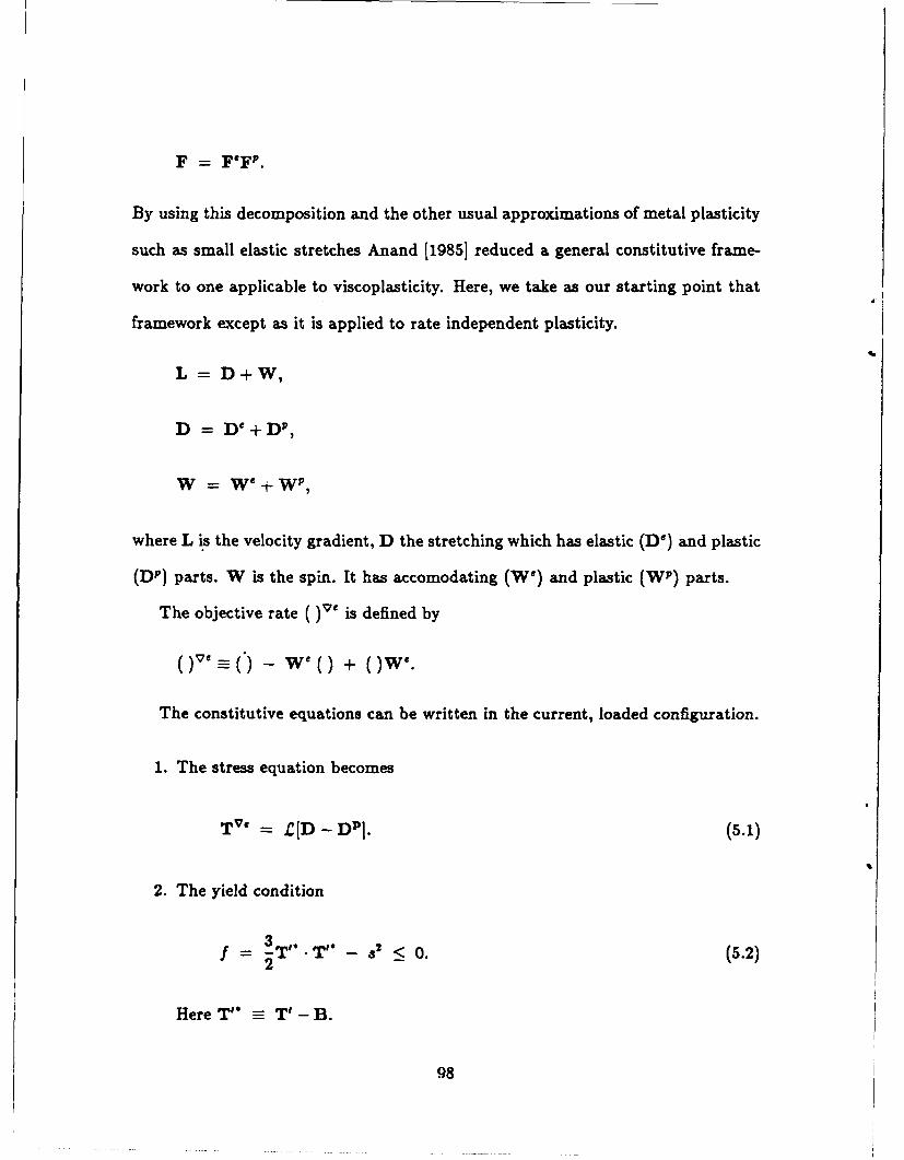
F = F'FP.

By using this decomposition and the other usual approximations of metal plasticity

such as small elastic stretches Anand [19851 reduced a general constitutive frame-

work to one applicable to viscoplasticity. Here, we take as our starting point that

framework except as it is applied to rate independent plasticity.

L = D+W,

D =D + DP)

W= We+W1,

where L is the velocity gradient, D the stretching which has elastic (D) and plastic

(DP) parts. W is the spin. It has accomodating (We) and plastic (WP) parts.

The objective rate ( is defined by

C -() - we() + ()w'.

The constitutive equations can be written in the current, loaded configuration.

1. The stress equation becomes

Tv. = £[D- DP]. (5.1)

2. The yield condition

3 I

f 3 - 2 < 0. (5.2)2

Here T'" T' - B.

98

3. The flow rule

DP= IV 1 (n. TV) n where n = T/(5.3)

= / T V ' ) !/P where fII (5B.-)T'*BW'~~~~ -- a (-bS(.

The parameter T provides the switching condition for plastic flow

if f =0 and n.L [D] > O then F=1,

if f'<0 or n-2[D]<O then -P=O.

4. The evolution equations

Bv' = C 1 DP - C, Z' B, (5.5)

i = Hi,.o f. (5.6)

Next we will turn our attention to functional forms to use for the scalar consti-

tutive functions C1, C2, H, H. 0 and 7. First, we can take advantage of the consis-

tency condition to relate C1, C2, Hjo, and H. The yield condition must be satisfied

throughout active plastic flow. We can write that by

.f = 3(T'- B). (Tve - B v ' ) - 2si = 0. (5.7)

If we substitute from the constitutive equations above (eqs. 6.35 to 6.38) and

simplify then we obtain the relation

H = 2 Hio + C, - C2 B-n. (5.8)3

99

In physical terms, this merely states that the total hardening is the sum of that

due to the isotropic expansion and that due to the kinematic translation. There are

differing views in the literature as to which of the material functions should be the

dependent one. If the emphasis of a model is on determining the evolution equations

then H is the dependent function and is determined from the evolution equation

functions via Equation 6.40. Dafalias [1984b] discusses these issues and stresses the

importance for correctly determining the plastic modulus H. In the present work

we view correctly choosing functions that can be experimentally verified as of prime

importance. Since, as we shall see, H can be directly determined from a uniaxial

experiment we will consider it an independent function and use the consistency

condition to infer one of the evolution equation functions.

5.3 Function Dependence

The general model presented in the previous section (Equations 6.33 to 6.38) is sim-

ilar to ones presented in the literature. It contains five constitutive scalar functions

(four of which are independent).

H: the plastic hardening modulus,

H ,,: the isotropic hardening modulus,

C1: the back stress hardening modulus,

C 2: the back stress recovery modulus,

q: the plastic spin factor.

Various models in the literature can be fit into the above framework.

100

* Classical Isotropic Hardening

H= !Hi 0 (P

3= 80

H,.o = 148.o(?)

C1' = C2 = 17 = 0

* Prager Kinematic Hardening

H= C,

H.o = 0

cl= c51( P)

C2 =0

77=0

* Krieg Combined Hardening

H = H(?)

Hio= 103H

C, = (1 -,3)H

C 2 =7 = 0

* Loret Model

H = fti*0(zp)

C1 = CZP)

C2 = &(,p)

101

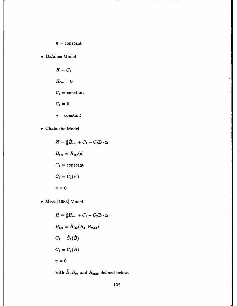
17 = constant

" Dafalias Model

H= C,

Hio = 0

C, = constant

C2 =0

17 = constant

" Chaboche Model

H o l +k C - C2B n

Hs,.o = fI,.o(s)

C, = constant

C2 =

" Mroz [1983] Model

H= !Hjo + C, - C2B . n

Ho = .iuo(Ba, Bmaz)

c, = &I (b)

C2 = &2(b)

with B, B., and B,,. defined below.

102

This s.mmary presents the simplified forms that various authors have used to

apply their models (often just for illustration). Here we need to consider the actual

material behavior and describe how proper dependence of these material functions

can model that behavior.

In continuing the state variable approach to modeling, we require that the scalar

material functions must be functions of the scalar list derivable from the state

variables T,B and s. Notice from above that many models require the various

moduli to depend upon the accumulated plastic strain. Since F is not a state

variable, we do not use it.

A general scalar list of invariants for constructing tensor representation functions

is given by Wang [1970] and applied to anisotropic hardening by Loret [19831. The

reduced list we want to consider here is drawn from that work with one addition.

I = {&, Bs, B

where

is the effective equivalent stress T= - B) . (T'- B)}2

is the effective back stress, B = {B . B},

s is the isotropic variable,

B,. is the maximum value that B has achieved over the history of deforma-

tion and is given by B,,. = Sup[].

The introduction of the variable B,,.. is motivated by the observation that

during stress reversal the hardening transient is limited to the time that it takes

for the back stress to reverse and achieve the same magnitude that it had prior to

103

unloading [Wilson and Bate, 1986]. The material remembers its previous extreme

state. This variable was first used by Mroz [1983]. He also allowed the possibility

for a material to cyclically soften by postulating an asymptotically limiting value

of the isotropic variable a. This limiting value was a function of B,. as well as a

certain accumulated back stress measure B4 .

This scalar variable list can be reduced for rate-independent plasticity. In this

case, whenever we are in a plastic loading situation contact with the yield surface

is required (9 s). We reduce the list to

t , B, .}.

Note that for viscoplasticity this reduction is not required or, in general, possible.

5.4 Furnctional Dependence

We can now synthesize the experimental observations from the literature that were

discussed in detail in Chapters 2 and 4 with the model framework established this

far in this chapter.

5.4.1 Back Stress Evolution

The back stress should increase monotonically under uniaxial, monotonic loading

until it reaches its saturation value. This can be achieved by having C1 and C2

be constants. The problem with that is the reversing behavior is generally not

matched well. In this model C2 sets the time constant for transition as the back

stress increases monotonically as well as the rate of transition during reverse flow.

G .aerally, the reverse transient occurs much more quickly than the hnitial build up.

Chaboche and Rousselier [1983] added several back stress variables having different

104

C2's to account for this (see Section 2.2.3). Mroz [1983] proposed using a different

C, for reverse loading than had been used for the monotonic build up.

The approach taken here is to take advantage of the fact that the variable B,,

can be thought of as defining a surface in back stress space. This is similar in form

to the yield surface in stress space. The surface can be defined by

2=f({-B.B}-B 2 OB - B ,B ma = 0.3

Similar to isotropic hardening plasticity, the surface just expands without trans-

lation or distortion. B,, is not a state variable for which there is a separate

evolution equation postulated. It merely tracks the maximum of B obtained during

deformation. By introducing this surface we have an easy way of delimiting when

the material is experiencing a reversing event (B inside of fB) and when the re-

versing transient is over (B returns to fE). Use of a surface provides for multiaxial

applica tion. This concept is illustrated in Figure 5.1 .

The moduli during the reversing event should depend upon the position of B

within fa. In some ways this can be reminiscent of the two surface plasticity

models where the moduli depend upon the relative positions of the two surfaces.

In those models elaborate updating procedures are required for determining the

current and initial distance measurements upon which the moduli depend. Here a

simple measure is used. It is the fractional distance that the back stress has moved

across the maximal back stress surface. In Figure 5.1 this fraction is illustrated as

g(g= - , 0 < g < 1). At the beginning of reverse flow g = 0 and as the reversing

transient ends B goes to the surface fB and g goes to 1.

A reverse loading event begins when ab = B,., and B • DP < 0. It continues

while ob < B,,, and concludes when ab -

105

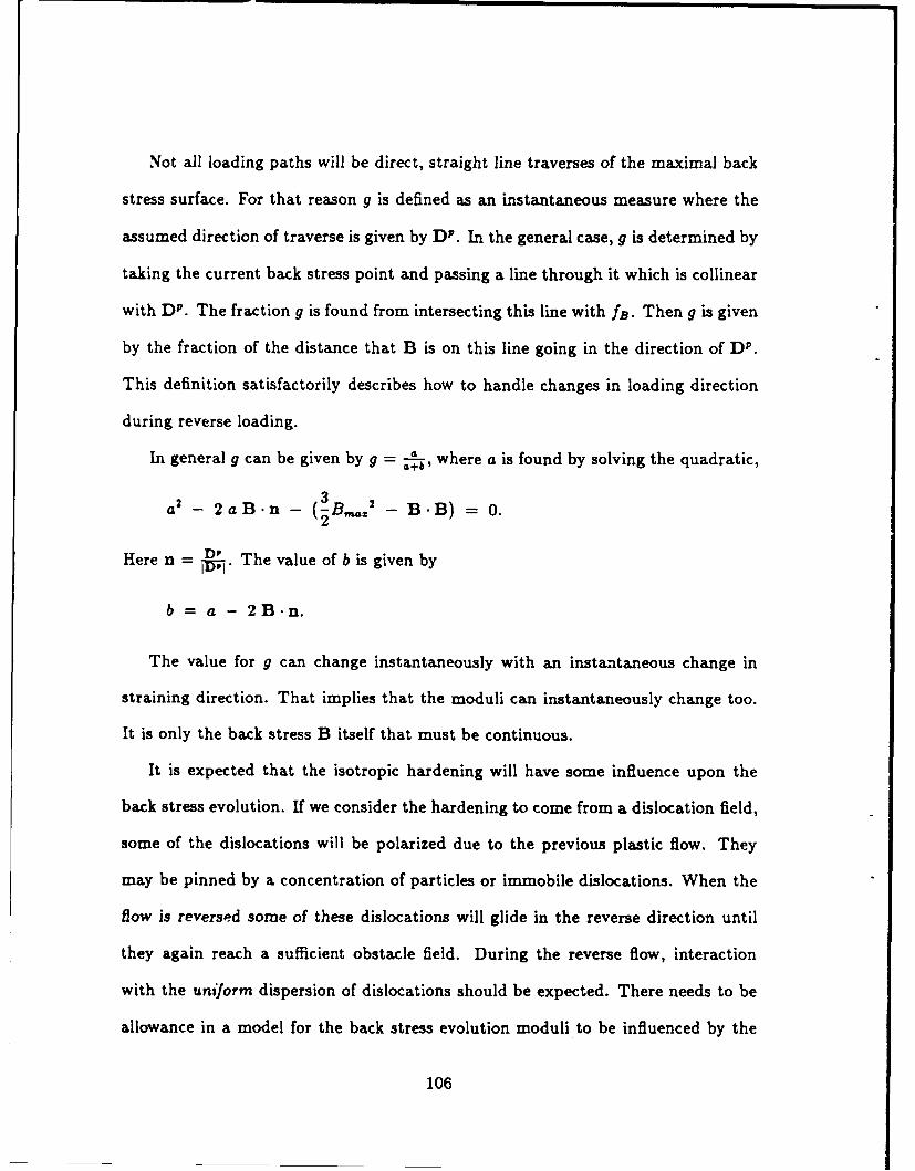
Not all loading paths will be direct, straight line traverses of the maximal back

stress surface. For that reason g is defined as an instantaneous measure where the

assumed direction of traverse is given by D P. In the general case, g is determined by

taking the current back stress point and passing a line through it which is collinear

with DP. The fraction g is found from intersecting this line with fB. Then g is given

by the fraction of the distance that B is on this line going in the direction of DP.

This definition satisfactorily describes how to handle changes in loading direction

during reverse loading.

In general g can be given by g = +, where a is found by solving the quadratic,

a' 2aB.n -( B,,. 2 -B.B) = 0.2

Here n . The value of b is given by

b=a-2B.n.

The value for g can change instantaneously with an instantaneous change in

straining direction. That implies that the moduli can instantaneously change too.

It is only the back stress B itself that must be continuous.

It is expected that the isotropic hardening will have some influence upon the

back stress evolution. If we consider the hardening to come from a dislocation field,

some of the dislocations will be polarized due to the previous plastic flow. They

may be pinned by a concentration of particles or immobile dislocations. When the

flow is reversed some of these dislocations will glide in the reverse direction until

they again reach a sufficient obstacle field. During the reverse flow, interaction

with the uniform dispersion of dislocations should be expected. There needs to be

allowance in a model for the back stress evolution moduli to be influenced by the

106

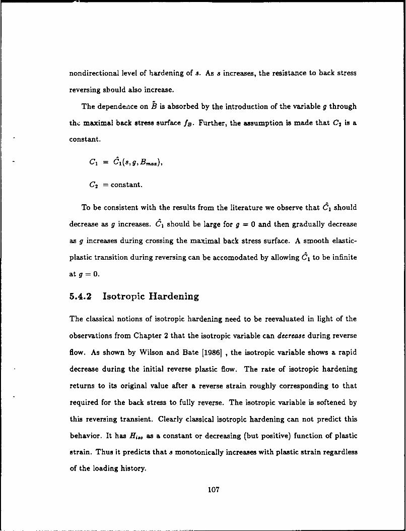
nondirectional level of hardening of s. As .9 increases, the resistance to back stress

reversing should also increase.

The dependence on B is absorbed by the introduction of the variable g through

the maximal back stress surface fB. Further, the assumption is made that C 2 is a

constant.

C, = j(sgBmaz),

C2 = constant.

To be consistent with the results from the literature we observe that C1 should

decrease as g increases. d, should be large for g = 0 and then gradually decrease

as g increases during crossing the maximal back stress surface. A smooth elastic-

plastic transition during reversing can be accomodated by allowing 6 1 to be infinite

at g = 0.

5.4.2 Isotropic Hardening

The classical notions of isotropic hardening need to be reevaluated in light of the

observations from Chapter 2 that the isotropic variable can decre ae during reverse

flow. As shown by Wilson and Bate [1986] , the isotropic variable shows a rapid

decrease during the initial reverse plastic flow. The rate of isotropic hardening

returns to its original value after a reverse strain roughly corresponding to that

required for the back stress to fully reverse. The isotropic variable is softened by

this reversing transient. Clearly classical isotropic hardening can not predict this

behavior. It has H,, as a constant or decreasing (but positive) function of plastic

strain. Thus it predicts that s monotonically increases with plastic strain regardless

of the loading history.

107

The way to model the observed behavior is to let Hi,, incorporate both hardening

and softening. This can be done by writing

Hao = hi - h21

where h, is the hardening function and h2 is the softening function. What is in-

tended here is not softening due to thermally assisted static recovery such as found

in viscoplastic models but rather dynamic recovery during reverse flow. The re-

verse flow erases some of the previous hardening. This can be envisioned from a

mechanism such as dislocation annhilation.

This softening is a new concept but it follows very logically from the experimental

results of Wilson and Bate [1986], Hasegawa et al. [1975], Marukawa and Sanpei

[1971], and Feltner [19631. Lowe and Miller [1983,1984] also made the observation

that during a large strain (±15% strain) hysteresis loop the isotropic component

softens slightly. They introduce a new scalar and a new tensor internal variable to

model this softening.

By separating Hi,,, additively we present a competition between two mechanisms,

one for hardening and one for softening. Some of the implications of this will be

discussed later.

The softening function is only operative during a reversing event. It is zero

for monotonic loading histories. Thus h, can be determined from simple tensile

or compressive experiments. Here we let h, be a function only of s, the isotropic

variable.

hi = I s)

This is sensible if we envision the isotropic resistance arising mainly from dislocation

interaction. The creation and tangling (or forest hardening) of dislocations provides

108

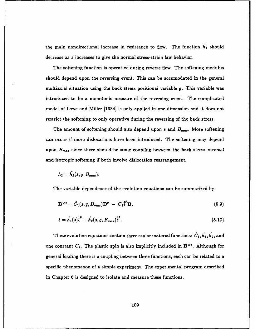
the main nondirectional increase in resistance to flow. The function h1 should

decrease as s increases to give the normal stress-strain law behavior.

The softening function is operative during reverse flow. The softening modulus

should depend upon the reversing event. This can be accomodated in the general

multiaxial situation using the back stress positional variable g. This variable was

introduced to be a monotonic measure of the reversing event. The complicated

model of Lowe and Miller [1984] is only applied in one dimension and it does not

restrict the softening to only operative during the reversing of the back stress.

The amount of softening should also depend upon a and B,,,.. More softening

can occur if more dislocations have been introduced. The softening may depend

upon B,.. since there should be some coupling between the back stress reversal

and isotropic softening if both involve dislocation rearrangement.

h2 h 2 (8,g, B..~).

The variable dependence of the evolution equations can be summarized by:

B"e = C1(s,g,B,.,)D P - C2 EB, (5.9)

= h1(s)i- h2(S, g, B,,,)- P. (5.10)

These evolution equations contain three scalar material functions: C1 s 1, /,/, and

one constant C2. The plastic spin is also implicitly included in BV'. Although for

general loading there is a coupling between these functions, each can be related to a

specific phenomenon of a simple experiment. The experimental program described

in Chapter 6 is designed to isolate and measure these functions.

109

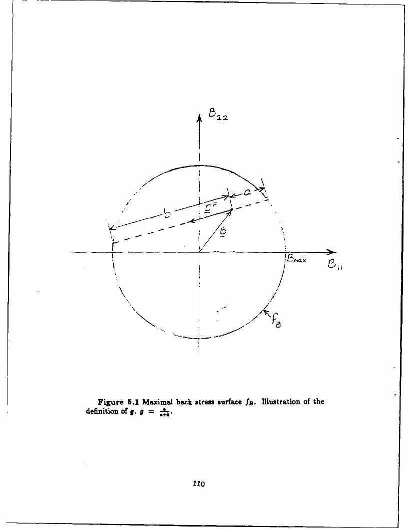
defintion f g. = -I

1103

If/

i j /

7i

Figure 5.1 Maximal back stress surface f's. illustration of thedefinition of g. g --=_.

110

Chapter 6

Experimental Program

6.1 Types of Experiments

In order to evaluate the multiaxial response of any material a variety of experiments

is needed. This is to assure that the results are not testing mode dependent. For

example, the uniaxial behavior of certain high strength steels depends upon whether

the testing is done in tension or compression (strength differential effect). If a model

is intended to apply to both of those loading environments then adequate data must

be available about both modes to allow construction of the model.

In this current program the following tests were conducted: tensile testing, large

strain compression testing, reverse strain testing, cyclic testing, and large strain

torsion testing. These tests were chosen to display as much of the phenomena of

rate-independent plasticity as possible. We can associate the observed phenomena

with approximate strain regimes. Evaluation of yield point and initial hardening

modulus are restricted to the first percent or two of strain and can be evaluated

from the uniaxial tensile test. The generation of back stress and development of

permanent softening upon strain reversal are associated with the first 10 to 15

percent strain. This regime can be studied by reverse strain and cyclic testing.

111

The decrease of the hardening modulus with plastic strain is evaluated from the

large strain compression test. Finally, more complex interactions of finite strains

and rotations causing nonproportional loading can be investigated using the torsion

test. Each of these testing types will be discussed in more detail below.

6.2 Materials Tested

Two metals were chosen for evaluation: 1100-0 aluminum and 316 stainless steel.

Complete data, generated from the types of tests outlined above, are not available in

the literature for any material. These two were chosen since they would be expected

to span a variety of behaviors in other metals.

The 1100-0 aluminum is a relatively simple, high stacking fault, face centered

cubic metal which is known to harden primarily by cell formation. It is not expected

to generate a large back stress since it has many slip systems to distribute the

deformation. The material was received from ALCOA in 11 inch diameter rods in2

the "F" condition. It was then annealed at 500 0C for 1 hour and allowed to air

cool. The 1100 aluminum that was tested came from two separate batchs although

both were annealed. The compression and torsion specimens came from one batch

(batch A). The reverse loading specimens came from another batch (batch B). The

final grair, structure is shown in Figure 6.1. The grains were equiaxed with an

approximate diameter of 70 microns.

The AISI 316 stainless steel belongs to the class of austenitic stainless steels so

it also has an FCC crystal structure but with a relatively low stacking fault energy

(781y) (Peckner and Bernstein [19771). The low stacking fault energy inhibits cross

slip and can be expected to generate a larger back stress. The material was received

112

in 1 1 inch diameter rods. It was annealed in air at 1075°C for 1 hour then air cooled.

The final grain structure is shown in Figure 6.2.

6.3 Experimental Apparatus

All of the experiments were conducted at ambient conditions. The equivalent strain

rate was nominally ' = 1 x 10-sec- 1 for all of the tests. These materials are

reasonably rate insensitive at room temperature and slow strain rate.

The experiments were conducted primarily using two servohydraulic test ma-

chines manufactured by Instron Corp. The uniaxial tests (tension, compression,

reverse straining, cyclic) were run on a 1331 testing machine controlled by an 8000

series computer based controller. The machine capacity was 100 KN (22,500 lbf).

Two load cells were used depending upon the experiment. A 10 KN cell was used

for the tensile and reversed loading tests of the 1100-0 aluminum and a 100 KN

cell for all of the other tests.

The torsion experiments were conducted on an Instron 1323 biaxial test machine

located at the U.S. Army Materials Technology Laboratory in Watertown, Mass.

This machine has a capacity (and load cell) of 50,000 lbf thrust and 25,000 in-lbf

torque. The machine was controlled using its analog function generator.

The data collection for both machines was via IBM personal computer based

systems using Metrabyte conversion boards. The collection for the torsion machine

used Keithley software while the system for the uniaxial machine used the Un-

kelscope program developed by Prof. W. Unkel at M.I.T. Approximately 500-1000

data points were collected for the uniaxial tests and 1000-2000 data points for the

torsion tests. All data were transferred to a Data General MV 10,000 supermini-

113

computer for reduction and comparison with theory.

6.4 Compression Testing

The use of compression tests to obtain large strain flow stress results has been

well documented [ASTM Standard E209-65; Chait and Papirno, 1983]. This test-

ing mode offers resistance to the necking geometric instability of the tension test

although it has special considerations of its own.

A circular cylindrical specimen is compressed between parallel flat platens.

Proper lubrication between platen and specimen is necessary to prevent barrelling

of the specimen. Homogeneous deformation can be achieved by proper selection

of the lubricant and the specimen geometry. In this study sheets of 0.003 inch

thick teflon were used to provide lubrication between polished steel platens and the

specimen. The specimen was simply a right, solid circular cylinder having smooth

ends. With certain lubricants, some investigators have grooved the ends of their

specimens to capture the lubricant [Brown 1987]. Grooving was used here during

some preliminary testing when Molydisulfide was being considered as the lubricant

but better results were obtained with smooth-end specimens and two layers of the

teflon sheets as the lubricant.

The aluminum compression tests were all conducted at a true strain rate of

i = 1 x 10- 3 sec-1 . This was achieved using an analog function generator designed by

M. Haghi [Haghi, 1987]. The actuator was controlled to move with an exponentially

decaying velocity to keep the logarithmic strain rate constant (i). The 316 stainless

steel compression tests were conducted both controlling the logarithmic strain rate

and controlling engineering strain rate (.). No differences were observed in the

114

material response to the two controlling methods.

Another experimental difficulty with the compression test is the tendency for

the specimen to shear. When the gauge length is too long or the platens are not in

good alignment the specimen will not deform uniformly but will shear. This mode

is reminescent of simple shear between the platens with evidence of some rollover

at diagonally opposite corners of the specimen. This unfavorable condition was

avoided by using specimens with an aspect ratio (original length divided by original

diameter) of 1.5 or less. For the tests run here the specimen dimensions were:

Table 6.1 Compression Specimen DimensionsMaterial Diameter (ram) Length (mm)

1100-0 aluminum 11.3 17.6316 stainless steel 6.4 9.0

The loads were directly measured from the load cell. The strains were deter-

mined from the displacement of the actuator with proper account taken for system

compliance. For the 1100 aluminum results the actuator displacement was taken

from the LVDT output of the actuator position. A nonlinear load train compliance

was measured by loading up the system without having a specimen in place. The

strains determined from this procedure matched well with results where a specimen

was strain gauged and tested. The strain gauge popped off after a small amount of

strain ( 5%) but provided an independent check that the strain measurements from

the actuator position were reasonable.

For the 316 stainless steel tests, instead of using the actuator LVDT output a

20% extensometer was placed across portions of the platens. This gave a stiffer

system for displacement measurement. Some platen compliance still had to be

subtracted off but it could be considered to have constant stiffness at the load levels

115

of the test.

The compression tests were successfully run to large strain with the above pre-

cautions. A strain of almost 95% was reached for the aluminum and 65% for the

stainless steel.

6.5 Reverse Straining Testing

In order to model the Bauschinger effect and general cyclic behavior of the materials

a certain number of reverse loading tests is required. These tests have typically been

done either by twisting a cylindrical specimen in one direction then reversing the

direction of twist or by loading in tension followed by compression. In this study,

tension/compression loading was used.

The proper measurement of reverse loading phenomena requires care in system

alignment. When a specimen is taken from tension to compression or vice-versa,

system backlash and misalignment can cause spurious results.

The testing system used was one designed for reverse loading and low cycle fa-

tigue. An Instron 1331 servohydraulic test machine was mounted with a Wood's

metal grip for system alignment. The specimen was a threaded, cylindrical sample

having a short gauge length, see Figure 6.3. The reduced gauge section was neces-

sary to prevent plastic buckling during compression. The specimen was threaded

into the top grip which was attached to the load cell. The specimen was firmly

locked in place using a differential nut assembly which preloaded the specimen

threads. With the specimen secure in the top assembly the alignment with the

actuator axis was checked using a dial gauge. The bottom of the specimen was

threaded into the Wood's metal grip assembly which was locked onto the actuator.

116

The grip allows for good alignment because it has two parts. One firmly attaches

to the actuator. The other attaches to the specimen, preloading the threads using

a differential nut. When installing the specimen the two components are free to

rotate and move relative to each other. Once the specimen is threaded into the grip

a low melting point liquid metal is allowed to cool and solidify locking the com-

ponents together without introducing bending moments to the load train. Thus

the specimen is securely fixed between the load cell and actuator, without bending

moments, and in line with the actuator axis.

The specimens deformed maintaining good alignment overall. Some of the 1100

aluminum specimens showed a shear across the gauge section at later parts of the

compressive loading. The data for this continued deformation after alignment was

lost has not been used.

The deformation was measured by attaching a 20% axial extensometer across the

gauge section. The loads were measured directly from the load cell and the results

converted to true stress and true strain based upon the extensometer output.

The reverse loading tests were limited in strain range to +20% and -5% so

separate tensile tests were run to expand this strain range. The tensile tests were

run with the same setup as was used for reverse loading. The only difference was

that the specimens were modified to have longer gauge lengths. The gauge length for

the stainless steel specimen was 29.2 mm (1.15 in) and for the aluminum specimen

was 38 mm (1.5 in).

117

6.6 Finite Element Analysis of Reverse StrainingSpecimen

The choice of specimen design for the reverse straining tests was based upon ex-

perience in the literature with specimens that could be used both for tensile and

compressive loading. In the course of analyzing the reverse straining results it was

noticed that the uniaxial loading flow stress level was higher for each of the reverse

tests than for the tension test having a longer gauge section. In order to investigate

the uniformity of stress and strain in the reverse loading specimen a finite element

analysis was conducted of the stainless steel specimen. The specimen dimensions

are shown in Figure 6.3.

Only one quadrant of the axisymmetric specimen was examined due to symme-

try. The region was divided up into 260 elements (4 node, bilinear, quadrilaterals),

Figure 6.4. The bottom row of nodes was fixed. The centerline row of nodes (on

the left in Figure 6.4) was restrained against radial displacement and the nodes at

the top were displaced vertically to simulate loading. The model had 594 degrees of

freedom. The material was treated as elastic-plastic with a Young's Modulus of 30

x 106 psi, Poisson's ratio v = 0.3, yield stress of 41,000 psi and a constant plastic

hardening modulus of 2.63 x 106 psi. The classical, isotropic hardening plasticity

relations were used. The analysis was conducted with the ABAQUS finite element

code using the nonlinear geometry option [ABAQUS, 19841.

One intent of the analysis was to compare the stress and strain distribution

inside the specimen gauge region with the homogeneous states assumed in reducing

the test data. In Figure 6.5 is plotted contours of constant vertical normal stress.

This is the stress that is assumed to be constant over the gauge section in the simple

118

1-D analysis. Notice the stress gradient along the specimen length in the shoulder

region. There is an area of elevated stress along the specimen axis approximately

one radius below the shoulder/gauge section transition. Across the very center of

the gauge section (the bottom of Figure 6.5) the vertical stress is fairly uniform

here being approximately 60 ksi for this moderate deformation.

The simple experimental analysis would take the total force on the specimen

and divide it by the average cross sectional area of the gauge section to give the

applied stress. Here we can see that the true stress is not constant throughout the

gauge region by varies due to the presence of other stress components. Along the

specimen central cross section the vertical stress is quite uniform so on this plane

the simple analysis would be a reasonable estimation of the vertical normal stress.

In Figure 6.6 the contours of constant accumulated plastic strain are shown.

Notice the continued gradient along the specimen length throughout the gauge sec-

tion. Experimentally an axial extensometer was used to determine the average

strain across the entire gauge section. The nominal gauge length of the exten-

someter was 0.5 inch. For the realistic deformation level shown here that means

averaging over strains that vary from about 3% to 9%. That gives a rough estimate

of the strain level. A better experimental technique would be to use a diametral

extensometer mounted at the center of the gauge section. Across this plane the

strain varies from 7% to less than 10%, a much tighter range than over the en-

tire gauge region although this is still less uniform than would be hoped. This is

an important experimental improvement. A diametral extensometer provides more

accurate behavior for these short gauge length specimens.

In order to compare the real material behavior with that which would be exper-

119

imentally determined from this specimen the finite element results were used. The

displacement of the node corresponding to the extensometer measured displacement

and the reaction forces corresponding to the load cell output were used as though

they were experimental data and the stress-strain behavior was computed.

Figure 6.7 shows the curve of equivalent stress versus equivalent strain. The base

curve is the elastic-plastic behavior input into the finite element model. This is the

material law seen at each point in the specimen. The curves marked Extensional and

Diametral show the average specimen behavior that would have been determined

experimentally using either an extensional or diametral extensometer, respectively.

The extensional curve lies well above the true material behavior and even the di-

ametral results are high. This is mainly due to the way the strain measurement was

necessarily averaged over the nonuniform gauge region using an extensometer.

In this experimental program the results that were observed are consistent with

this analysis. The flow curve for all of the tests run with this specimen design

having a short gauge length were higher than the results for a tensile test with a

longer, more uniform, gauge length. To compensate for this elevation in apparent

flow stress the reverse loading stresses were reduced to agree with the tensile data.

The procedure used was as follows:

1. The forward flow stress a! at the point of reversing the straining direction,

e1, was determined.

2. The flow stress from the tensile test was evaluated at the same strain leveltenC.

3. The stress multiplier was defined by SMULT -

120

4. The stresses for the entire data set from that reverse loading experiment were

multiplied by SMULT.

This brings all of the reverse loading curves to a common basis. This procedure

not only accounts for the stress nonuniformity in an approximate way but it also re-

moves any systematic experimental error from the flow stress measurements. Types

of error that this would correct include: load cell calibration variability, specimen

geometry variability, and material differences between specimens.

From the results in Figure 6.7 we can see that a better way to use this type of

specimen design would be with a diametral extensometer. The stress and strain are

more nearly uniform across the central cross section than they are throughout the

whole gauge section. Future testing should be conducted this way.

6.7 Torsion Testing

The torsion test holds a number of advantages for determining material behavior at

large strain. These advantages are discussed elsewhere but some of the main points

are again summarized here:

1. No large changes in the geometry of the specimen.

2. Multiaxial stress states are obtainable with both normal and shear stresses.

3. Constant strain rates can be achieved with simple ramp type control signals.

4. A deformation field having equal stretching and spin components is achieved.

5. There is noncoaxiality between the stress deviator and the back stress.

121

Torsion of cylindrical testpieces has been commonplace for a long time. Gen-

erally tests conducted on solid rods have been used. These produce nonuniform

stress and strain fields which vary in the specimen with radial position. The re-

quired torque to produce a certain twist angle is generally the output of this type

of test. Various techniques have been used to convert the torque/twist behavior to

stress-strain curves -([Dieter 1976, p. 3811, [Canova, Shrivastava, Jonas and G'Sell,

19821, [Shrivastava, Jonas and Canova, 1982]). These assume certain constitutive

restrictions and neglect the production of axial normal stresses and their interac-

tion with the shear deformation fields. At best, the results from solid rod testing

represents an averaged flow stress magnitude.

To circumvent these limitations Lindholm et al. [Lindholm, Nagy, Johnson and

Hoegfeldt, 19801 used a cylindrical specimen having a thin walled, tubular gauge

section. This allows a nearly uniform stress and strain distribution in the gauge

section. As long as the wall thickness is much less than the specimen's radius

the gauge region can be treated as a plane stress sheet. This design has been

extensively used for small strain, multiaxial testing but suffers plastic buckling when

compressed or twisted to large strain. Lindholm et al. reduced the gauge length of

their specimen and were able to obtain results up to shear strains of 700%. Since

that time this specimen design has received much attention but without extensive

experimental usage.

The feature of this specimen that is most striking is that it has a massive shoulder

very close to the gauge region. This restricts the axial deformation that the specimen

can be used for since an axial strain would also produce a hoop strain which would

be resisted at the shoulder. This would produce a large strain gradient since the

122

shoulder has such a small transition region close to the gauge section. This specimen

is best suited for a pure torsion test where the crosshead is fixed so that the axial

strain is zero and the deformation is nearly simple shear. This produces a simple

deformation field.

F= 0 ,01

where -y is the (engineering) shear strain in the gauge section.

I

where f is the mean radius of the gauge section, I is the gauge length, and WD is the

angle that the crosshead has twisted through. Note that is is important to fix the

crosshead against axial motion to ensure that the gauge section maintains uniform

deformation. Lipkin et al. [Lipkin, Chiesa and Bammann, 1987] have conducted a

finite element analysis of a Lindholm type specimen. For their constitutive model

of 304L stainless steel and particular specimen geometry they found that the shear

stress and shear strain were quite uniform through the wall thickness although

deformation was not constrained to just the gauge section but did extend somewhat

into the shoulder transition region at shear strains above -Y = 2.0. Also they found

that the gauge length did change somewhat even when they fixed the shoulders

against axial motion away from the gauge section.

The torsion tests conducted in this study also utilized Lindholm type specimens.

Figure 6.8 shows the geometries used for both the 1100 aluminum and the 316

stainless steel tests. The specimen dimensions are given in Table 6.2.

Table 6.2 Torsion Specimen Dimensions

123

Material Gauge Inside Outside ShoulderLength (mm) Diameter (mm) Diameter (mm) Diameter (mm)

1100 Alum 7.9 27.76 30.30 38.0316 SS 5.9 19.05 20.52 38.1

For the aluminum specimen a larger diameter and thicker wall was allowed for

the same total applied torque for both materials. For the stainless steel the ratio

of outside diameter to wall thickness is - = 28. The thin wall approximation is

appropriate for this ratio. The aluminum specimen had 22 = 24. This also is quite

good. Values for this ratio common in the literature are around 16 [Lipkin, Chiesa

and Bammann, 1987].

The specimens were gripped in an hydraulic collet pair of grips mounted on the

Instron 1323 biaxial test machine. Into the ends of each specimen were inserted mild

steel plugs that were match machined for tight fit. These plugs were inserted into

the specimen ends and extended approximately 1 to 1 of the way down the shoulder

region. Their purpose was to provide an extra support when the hydraulic collets

closed on the outside of the shoulder regions. The desire was to have the clamping

forces of the grips supported as much as possible by radial stress transmitted to the

plug and as little as possible by hoop stresses in the specimen which could more

easily influence the gauge region.

These grips were aligned in the loading frame when installed by dial gauges and

strain gauged solid rod specimens. The grips are very massive as seen in Figure 6.9

and were never used to their rated capacity. No slipping or backlash was observed

at any time with this set-up.

It is extremely important to have a gripping system which can hold good align-

ment throughout the test. For the large angles that the actuator is twisted through

any eccentricity of the specimen is greatly amplified. Also it is important to be able

124

to transmit both torque and axial force with no slippage or cross talk. Early in our

testing program we tried a gripping arrangement where the specimens were held

by cross pins. This was abandoned because the position where the pin and holes

contacted would change during loading as the ratio of torque to axial force changed.

This changed the axial position of specimen end and introduced an applied axial

normal strain.

The hydraulic collet grips did not suffer from the above problems and served

well as our method of gripping.

The torsion tests were conducted as follows:

1. The axial position of the actuator was held constant. The axial control channel

of the feedback system was set to maintain a constant axial position of the

actuator as measured by its LVDT.

2. The rotary motion of the actuator was controlled to maintain a constant rate

of twist. That twist rate was selected to give an equivalent strain rate in

the gauge section of - = V3 j = 1 sec'. The standard analog function

generator was used, and it satisfactorily controlled this motion.

3. The rotary position, axial force and torque were digitally recorded.

In reducing the data, this test was assumed to simulate simple shear. The system

was stiff and had massive grips and shoulders so all of the deformation was assumed

to occur in the gauge region. The strain and stresses were then given by:

I

T12 = Mrr,2- r, 2 )r'

125

T2 2= F_r( - 2),

where I is the gauge length, A4 the twist angle of the actuator, r,, r, the inside

and outside radii of the gauge section, r,. the mean radius (rm = 1(ri + r,)), M the

measured torque, and F the measured axial force.

Lipkin et al. [Lipkin, Chisea and Bammann, 1987] have questioned this type of

analysis for their specimen. They maintain that the proper strain state in the gauge

section may not be properly represented when the plastic deformation extends into

the transition region. For their tests this begins to be important at shear strains

around 2.0. In our work the largest shear strains to which we tested were around

1.6. Post test observation of the specimens did not show any permanent strain in

the transition region so these objections were set aside until after analysis of the

test results.

6.8 Experimental Results

In this section the results of the experimental program outlined above are presented.

These experiments were all completed at M.I.T. with the exception of the torsion

tests, as described above. The results are presented in terms of Cauchy stress and

true (logarithmic) strain.

Figure 6.10 shows the tensile test results for the type 316 stainless steel. The

material shows a rather abrupt yield with nearly linear hardening. Here we see the

substantial hazdening rate persists even to the maximum strain of the test (38%).

This alloy has good tensile elongation due to its large ductility and resistance to

necking from its high hardening.

The 1100-0 aluminum tensile results are displayed in Figure 6.11. Notice the

126

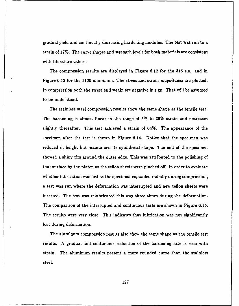
gradual yield and continually decreasing hardening modulus. The test was run to a

strain of 17%. The curve shapes and strength levels for both materials are consistent

with literature values.

The compression results are displayed in Figure 6.12 for the 316 s.s. and in

Figure 6.13 for the 1100 aluminum. The stress and strain magnitudes are plotted.

In compression both the stress and strain are negative in sign. That will be assumed

to be unde: tood.

The stainless steel compression results show the same shape as the tensile test.

The hardening is almost linear in the range of 5% to 35% strain and decreases

slightly thereafter. This test achieved a strain of 64%. The appearance of the

specimen after the test is shown in Figure 6.14. Notice that the specimen was

reduced in height but maintained its cylindrical shape. The end of the specimen

showed a shiny rim around the outer edge. This was attributed to the polishing of

that surface by the platen as the teflon sheets were pinched off. In order to evaluate

whether lubrication was lost as the specimen expanded radially during compression,

a test was run where the deformation was interrupted and new teflon sheets were

inserted. The test was relubricated this way three times during the deformation.

The comparison of the interrupted and continuous tests are shown in Figure 6.15.

The results were very close. This indicates that lubrication was not significantly

lost during deformation.

The aluminum compression results also show the same shape as the tensile test

results. A gradual and continuous reduction of the hardening rate is seen with

strain. The aluminum results present a more rounded curve than the stainless

steel.

127

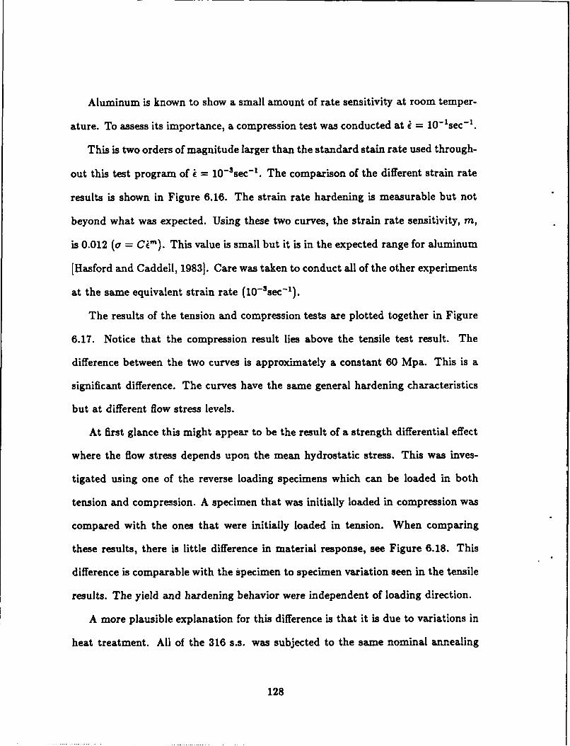
Aluminum is known to show a small amount of rate sensitivity at room temper-

ature. To assess its importance, a compression test was conducted at i = 10-1sec- 1.

This is two orders of magnitude larger than the standard stain rate used through-

out this test program of i = 10-sec - . The comparison of the different strain rate

results is shown in Figure 6.16. The strain rate hardening is measurable but not

beyond what was expected. Using these two curves, the strain rate sensitivity, m,

is 0.012 (a = Ci m ). This value is small but it is in the expected range for aluminum

[Hasford and Caddell, 1983]. Care was taken to conduct all of the other experiments

at the same equivalent strain rate (10-sec- 1 ).

The results of the tension and compression tests are plotted together in Figure

6.17. Notice that the compression result lies above the tensile test result. The

difference between the two curves is approximately a constant 60 Mpa. This is a

significant difference. The curves have the same general hardening characteristics

but at different flow stress levels.

At first glance this might appear to be the result of a strength differential effect

where the flow stress depends upon the mean hydrostatic stress. This was inves-

tigated using one of the reverse loading specimens which can be loaded in both

tension and compression. A specimen that was initially loaded in compression was

compared with the ones that were initially loaded in tension. When comparing

these results, there is little difference in material response, see Figure 6.18. This

difference is comparable with the specimen to specimen variation seen in the tensile

results. The yield and hardening behavior were independent of loading direction.

A more plausible explanation for this difference is that it is due to variations in

heat treatment. All of the 316 s.s. was subjected to the same nominal annealing

128

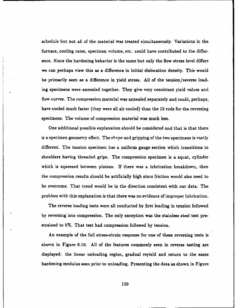
schedule but not all of the material was treated simultaneously. Variations in the

furnace, cooling rates, specimen volume, etc. could have contributed to the differ-

ence. Since the hardening behavior is the same but only the flow stress level differs

we can perhaps view this as a difference in initial dislocation density. This would

be primarily seen as a difference in yield stress. All of the tension/reverse load-

ing specimens were annealed together. They give very consistent yield values and

flow curves. The compression material was annealed separately and could, perhaps,

have cooled much faster (they were all air cooled) than the 15 rods for the reversing

specimens. The volume of compression material was much less.

One additional possible explanation should be considered and that is that there

is a specimen geometry effect. The shape and gripping of the two specimens is vastly

different. The tension specimen has a uniform gauge section which transitions to

shoulders having threaded grips. The compression specimen is a squat, cylinder

which is squeezed between platens. If there was a lubrication breakdown, then

the compression results should be artificially high since friction would also need to

be overcome. That trend would be in the direction consistent with our data. The

problem with this explanation is that there was no evidence of improper lubrication.

The reverse loading tests were all conducted by first loading in tension followed

by reversing into compression. The only exception was the stainless steel test pre-

strained to 5%. That test had compression followed by tension.

An example of the full stress-strain response for one of these reversing tests is

shown in Figure 6.19. All of the features commonly seen in reverse testing are

displayed: the linear unloading region, gradual reyield and return to the same

hardening modulus seen prior to unloading. Presenting the data as shown in Figure

129

6.19 does not bring out one of the important features of reverse testing though.

Often permanent softening is observed where the final flow stress after reversing

is smaller in magnitude than the continued forward loading would be. In order to

emphasize this, as well as compactly present the results from a number of tests, we

adopt a standard way to present the reversing data. For the reversing portions of the

curves only the compressive region is shown. It is displayed in the first quadrant

by plotting the absolute value of stress against an accumulated strain measure

where the elastic strain is added to the accumulated, effective plastic strain. This

effectively rotates the compressive stress-strain data by 1800 about the point during

unloading, of zero stress. Displaying the data this way allows easy comparison of

how the reverse yield has been lowered, the extent of rounding during reverse flow,

and the permanent softening.

There was small specimen to specimen variation in the forward loading flow

curves. this was compensated for by normalizing all of the reverse loading tests to

the tensile test. The procedure for this is discussed in section 3.6.

The reverse loading data are presented in Figure 6.20 for stainless steel and

Figure 6.21 for the 1100 aluminum. The data show the trends that would be

expected. The permanent softening first increases and then is fairly constant with

prestrain. This has been extensively noted in the literature (see Chapter 2). There

also is no abrupt yield during reversing.

One cyclic test was conducted. That involved 5 cycles of ±5% strain controlled

cycling. The resulting stress-strain response is shown in Figure 6.22. The material

quickly hardens to a saturation stress amplitude of about 750 MPa.

The final testing mode was in fixed end torsion of thin-wall tubular specimens.

130

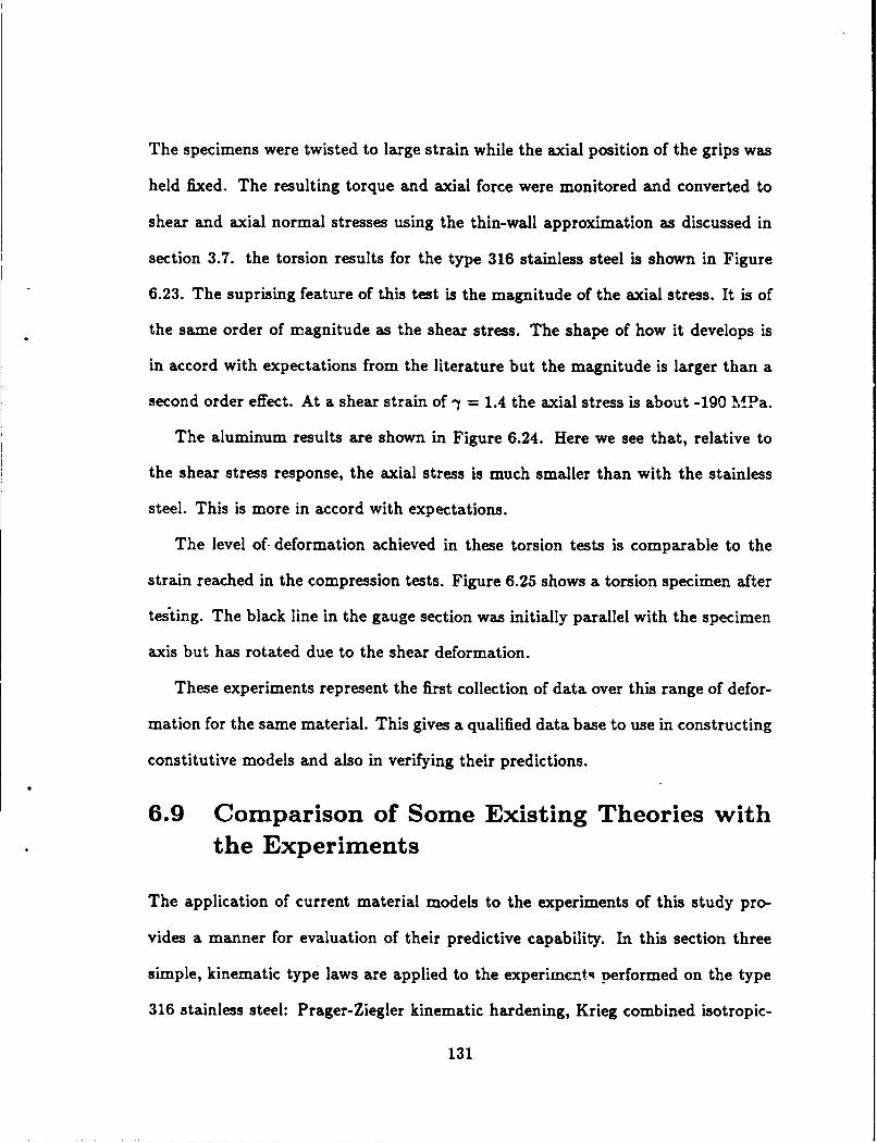
The specimens were twisted to large strain while the axial position of the grips was

held fixed. The resulting torque and axial force were monitored and converted to

shear and axial normal stresses using the thin-wall approximation as discussed in

section 3.7. the torsion results for the type 316 stainless steel is shown in Figure

6.23. The suprising feature of this test is the magnitude of the axial stress. It is of

the same order of magnitude as the shear stress. The shape of how it develops is

in accord with expectations from the literature but the magnitude is larger than a

second order effect. At a shear strain of -y = 1.4 the axial stress is about -190 .1.1Pa.

The aluminum results are shown in Figure 6.24. Here we see that, relative to

the shear stress response, the axial stress is much smaller than with the stainless

steel. This is more in accord with expectations.

The level of. deformation achieved in these torsion tests is comparable to the

strain reached in the compression tests. Figure 6.25 shows a torsion specimen after

testing. The black line in the gauge section was initially parallel with the specimen

axis but has rotated due to the shear deformation.

These experiments represent the first collection of data over this range of defor-

mation for the same material. This gives a qualified data base to use in constructing

constitutive models and also in verifying their predictions.

6.9 Comparison of Some Existing Theories withthe Experiments

The application of current material models to the experiments of this study pro-

vides a manner for evaluation of their predictive capability. In this section three

simple, kinematic type laws are applied to the experimcntq performed on the type

316 stainless steel: Prager-Ziegler kinematic hardening, Krieg combined isotropic-

131

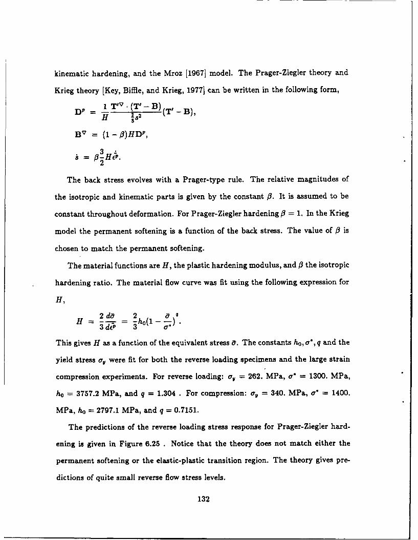
kinematic hardening, and the Mroz [1967] model. The Prager-Ziegler theory and

Krieg theory [Key, Biffle, and Krieg, 1977] can be written in the following form,

1 T 'V (T'- B)(T' -B),

B v = (1 - 3)HD P ,

# 3HEP.2

The back stress evolves with a Prager-type rule. The relative magnitudes of

the isotropic and kinematic parts is given by the constant P. It is assumed to be

constant throughout deformation. For Prager-Ziegler hardening #3 = 1. I. the Krieg

model the permanent softening is a function of the back stress. The value of P is

chosen to match the permanent softening.

The material functions are H, the plastic hardening modulus, and / the isotropic

hardening ratio. The material flow curve was fit using the following expression for

H,

2d 2

H = = h0(1-

This gives H as a function of the equivalent stress a. The constants h0 , a*, q and the

yield stress o were fit for both the reverse loading specimens and the large strain

compression experiments. For reverse loading: a. = 262. MPa, a* = 1300. MPa,

ho = 3757.2 MPa, and q = 1.304 . For compression: a. = 340. MPa, o* = 1400.

MPa, ho = 2797.1 MPa, and q = 0.7151.

The predictions of the reverse loading stress response for Prager-Ziegler hard-

ening is given in Figure 6.25 . Notice that the theory does not match either the

permanent softening or the elastic-plastic transition region. The theory gives pre-

dictions of quite small reverse flow stress levels.

132

In the Krieg theory, the introduction of isotropic hardening allows better match

of the reversing behavior. The isotropic ratio was chosen by predicting one of the

reversing curves and adjusting j3 to match the permanent softening. A value of

0 = 0.88 gave satisfactory agreement as shown in Figure 6.26 . This partitioned

the hardening to 88% isotropic and 12% kinematic. The application of this to the

rest of the reverse curves is shown in Figure 6.27. The permanent softening is well

matched but the transition is ignored and the gradually changing slope is replaced

with a sharp reverse yield.

The prediction from this model of the cyclic test is shown in Figure 6.28 . A

very "box like" response is predicted which saturates at a stress of 1300 MPa(= a*).

This does not agree with experiment.

Finally, the prediction of the torsion test is also examined in Figure 6.29 . The

agreement with experiment is still not close. The shear stress is overpredicted and

the normal stress is underpredicted.

The Krieg model can be made to match the permanent softening of a single

reverse by treating the back stress as a phenomenological fitting parameter. This

provides a reasonably good estimate of the reverse flow stress after several percent

reverse strain. This neglects the physics of the deformation as developed in the

main body of this work. The transition region is not modeled and it predicts that

all symmetric strain controlled cycling will saturate at the same stress level, a*.

The Mroz [1967] model is briefly described in Appendix B. It consists of nested

yield surfaces each of which has a different plastic modulus associated with it. This

model was applied to the type 316 s.s. experiments by segmenting the first 30%

strain from the tension test into 10 linear segments. This 10 surface model was used

133

to predict the reverse loading experiments. Figure 6.30 shows these results.

The Mroz model does not match the experiments very well. The permanent

softening is vastly overpredicted. The reverse predictions do not show the gradual

elastic-plastic transition because tensile test stress-strain behavior shows nearly

linear hardening. Since there is not much of a knee region during initial loading

then there can not be much of one during reverse loading using the Mroz model.

Here we have seen that none of these theories does a satisfactory job describing

the basic experiments. The next chapter applies the new modeling ideas developed

in this work to these experiments.

134

Figure 6.1 Micrograph of 1100-0 aluminum after annealing showinggrain structure.

17.o

Figure 6.2 Micrograph of type 316 stainless steel after annealingshowing grain structure.

135

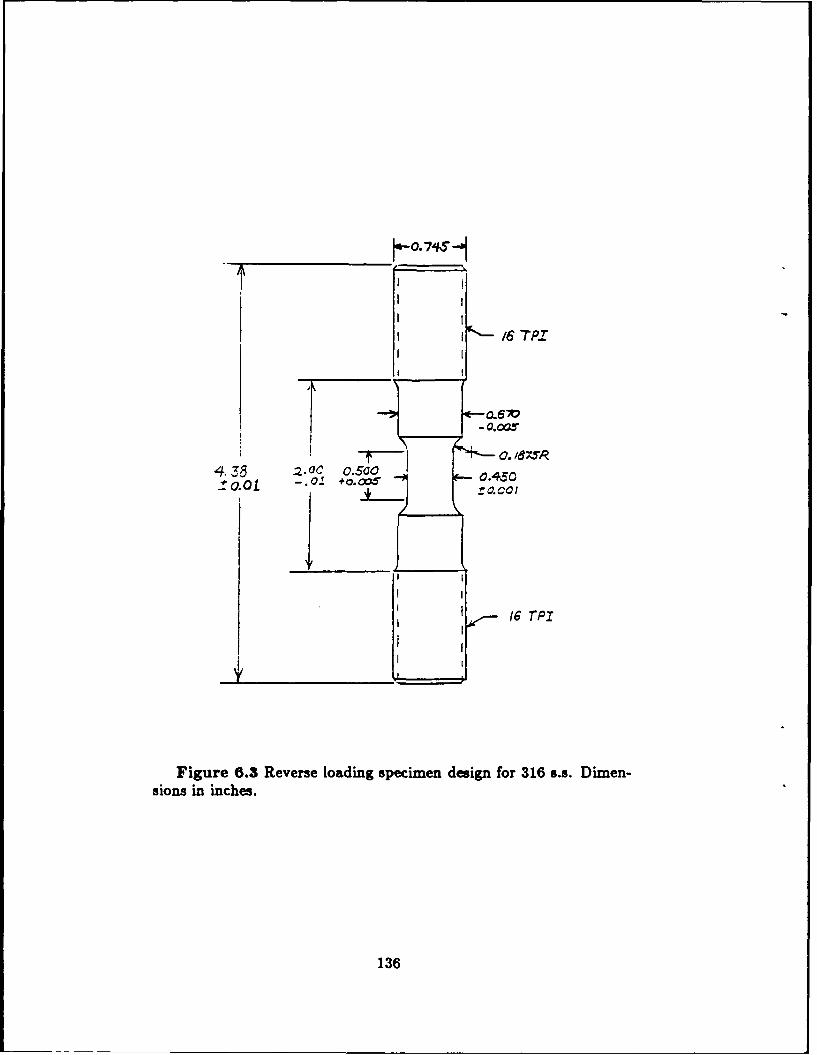
1 16 TPZ

.-O.002

0. /67$4.38 2OC 0.5040

.Of -. 01

Figure 6.3 Reverse loading specimen design for 316 s.s. Dimen-sions in inches.

136

Figure 6.4 Finite element mesh used to model the reverse loading

specimens. It contains 260 4-node elements.

137

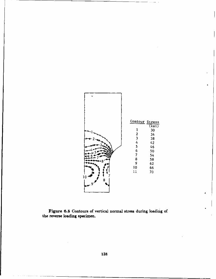
Contour Stress(ksi)

1 302 34

2 3 383 4 42

4 05 466 50

667 546 W7 8 58

8 9 62

10 6611 70

1078

QJI9

Figure 6.5 Contours of vertical normal stress during loading ofthe reverse loading specimen.

138

Contour Plastic Strain

1 02 0.01

1 3 0.024 0.035 0.046 0.05

7 0.068 0.07

2 9 0.083 4 10 0.09

6 11 0.10

7

9 8

-10-

Figure 6.6 Contours of accumulated equivalent plastic strain dur-ing the vertical loading of the reverse loading specimen.

139

Diametral

68888

rn 40880

8.80 8.82 8.84 8.06 8.08 0.18

Strain

Figure 6.7 Plot of average stress against average strain for thespecimen using different extensometer measures of strain.

140

141-

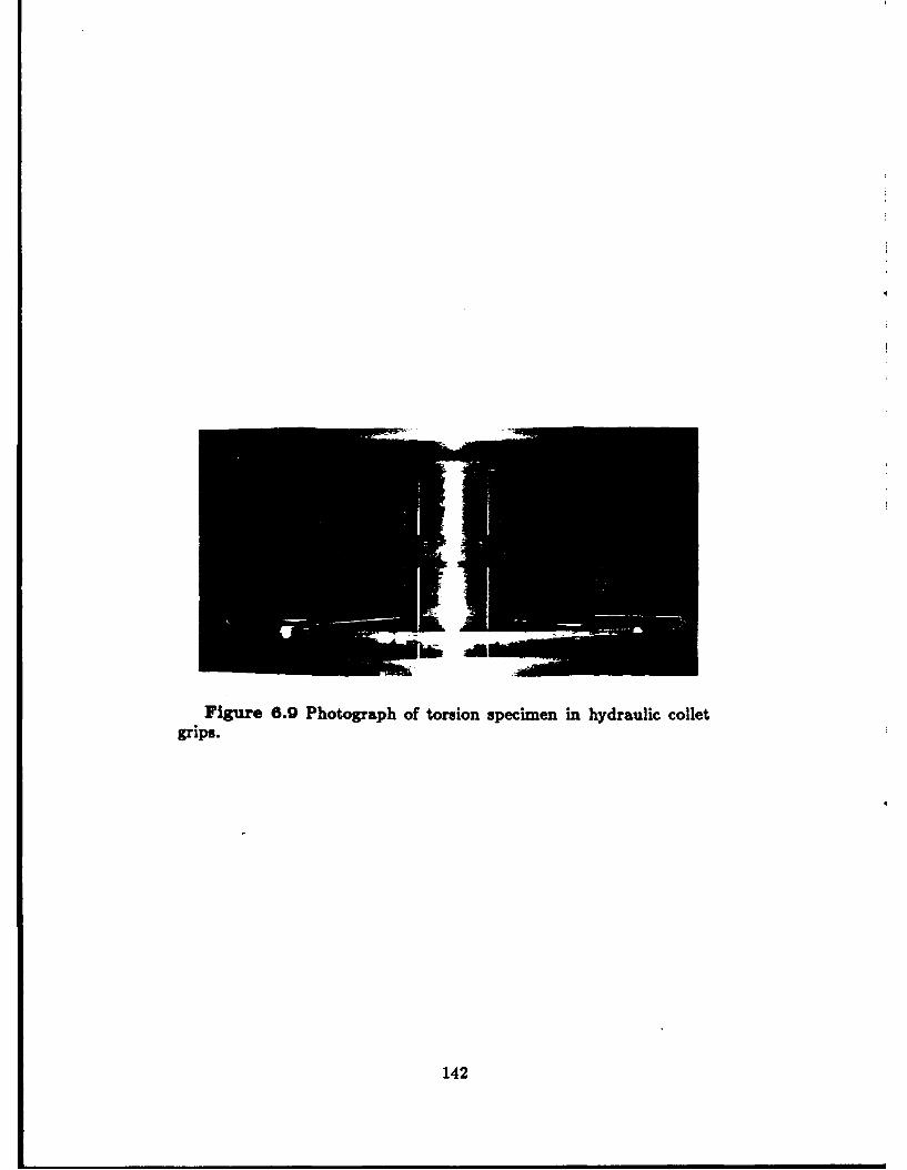
Figure 8.0 Photograph of torsion specimen in hydraulic colletgripe.

142

1000TENSILE TEST316 STAINLESS STEEL800

S 600

S 400

200

0.00 .05 0.10 0.15 0.20 0.25 0.30 0.35 0.40

STRAIN

Figure 6.10 Experimental stress-strain result for tensile test oftype 316 stainless steel.

143

125 *

TENSILE TEST

10 1100-0 ALUMINUM

~75

44 50

25

0 [ ... I

0.00 .02 .04 .06 .08 0.10 0.12 0.14 0.16 0.18

STRAIN

Figure 6.11 Experimental stress-strain result for tensile test of1100-0 aluminum.

144

1200 COMPRESSION TEST

316 STAINLESS STEEL1000

S 800

V 600

E- 400

200

0.0 0.1 0.2 0.3 0.4 0.5 0.6 0.7

STRAIN

Figure 6.12 Experimental stress-strain result for compression testof type 316 stainless steel.

145

175COMPRESSION TEST

150 1100-0 ALUMINUM

2 125

100

S 75

150

25

00.0 0.1 0.2 0.3 0.4 0.5 0.6 0.7 0.8 0.9

STRAIN

Figure 6. 13 Experiment al stress-strain result for compression testof 1100-0 aluminum.

146

-7w

71M

T

Figure 6.14 Photograph of deformed compression specimen of1100-0 aluminum. Final plastic equals -0.9.

147

1500

COMPRESSION TEST

1250 316 STAINLESS STEELRELUBRI CATED ..

1000

cn 750

500.,)

250

0.0 0.1 0.2 0.3 0.4 0.5 0.6 0.7

STRAIN

Figure 6.15 Comparison of compression results for two tests oftype 316 stainless steel. One test was run continuously using just theinitial teflon lubrication between specimen and platens. The othertest was interrupted two times to relubricate the specimen-platen in-terface.

148

175 COMPRESSION TEST150 I-.15 1100-0 ALUMINUM

_. -

1- 125

100

S 75

c-f 50

25

0.0 0.1 0.2 0.3 0.4 0.5 0.6 0.7 0.8 0.9

STRAIN

Figure 6.16 Comparison of compression test of type 316 stainlesssteel run at two different logarithmic strain rates (See- 1 ).

149

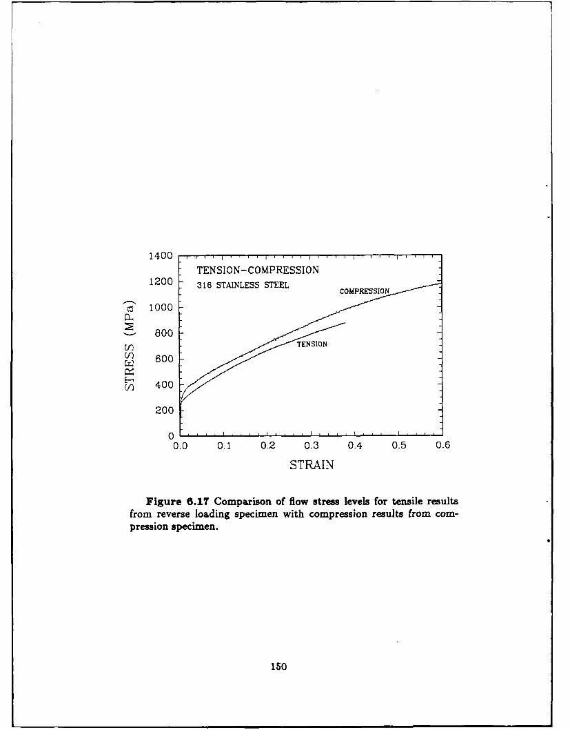
14 0 0 . . . . . , . . . . . . . . , . .

TENSION -COMPRESSION1200 316 STAINLESS STEEL

c 1000

800

) 600

E--o 400

200

0.0 0.1 0.2 0.3 0.4 0.5 0.6

STRAIN

Figure 6.1T Comparison of flow stress levels for tensile resultsfrom reverse loading specimen with compression results from com-pression specimen.

150

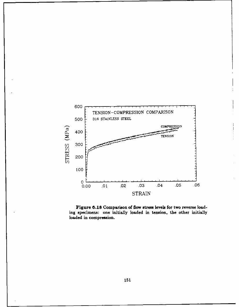
600TENSION-COMPRESSION COMPARISON

500 316 STAINLESS STEEL

COMPRESSION

,400

v) 300

200V-

100

0.00 .01 .02 .03 .04 .05 .06

STRAIN

Figure 6.18 Comparison of flow stress levels for two reverse load-ing specimens: one initially loaded in tension, the other initially

loaded in compression.

151

800

REVERSE LOADING TEST600316 STAINLESS STEEL

400

200. . . . .... . . . . . . . . . . . . . . . . . . . . . . . . . . . . . . . . . . . . .

-200

-400

-600

0.00 .02 .04 .06 .08 0.10

STRAIN

Figure 6.19 True stress-true strain result for type 316 stainlesssteel loaded in tension followed by compression.

152

700 Reverse Loading

600

:= 500

9I) 400

S300

93 200

100

0 .0.00 .05 0.10 0.15 0.20 0.25

STRAIN

Figure 6.20 Composite figure showing the reversing branches ofthe reverse loading tests of type 316 stainless steel. All of the revers-ing branches have been rotated into the first quadrant. The tensilecurve is also plotted for comparison of flow stress levels.

153

125REVERSE LOADING TESTS

00-1100-0 ALUMINUM ---- --100

: 75

c1n

4 5001

25

0 -1--- J- rrf"

0.00 .05 0.10 0.15 0.20

STRAIN

Figure 6.21 Composite figure showing the reversing branches ofthe reverse loading tests of 1100-0 aluminum. All of the reversingbranches have been rotated into the first quadrant. The tensile curveis also plotted for comparison of flow stress levels.

154

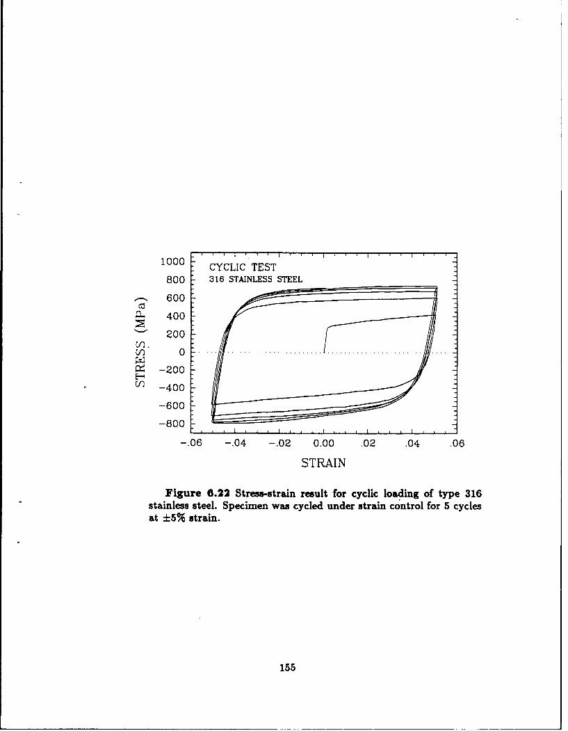
1000 CYCLIC TEST

800 316 STAINLESS STEEL

. 600

- 400

"'" 200

S-200Cfl -400

-600

-800

-. 06 -. 04 -. 02 0.00 .02 .04 .06

STRAIN

Figure 6.22 Stress-strain result for cyclic loading of type 316stainless steel. Specimen was cycled under strain control for 5 cyclesat ±5% strain.

155

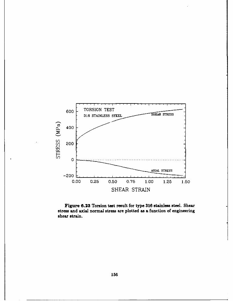
600 TORSION TEST316 STAINLESS STEEL SHE.aR STESS

S400

V)v) 200

E-oo 0 ........ .........................

-200 AULTRE,

0.00 0.25 0.50 0.75 1.00 1.25 1.50

SHEAR STRAIN

Figure 6.23 Torsion test result for type 316 stainless steel. Shearstress and axial normal stress are plotted as a function of engineeringshear strain.

156

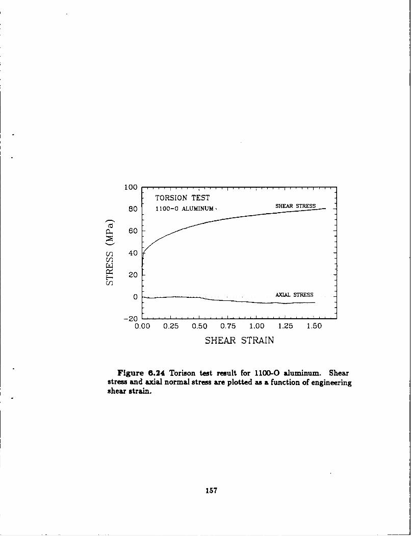
TORSION TEST

80 1100-0 ALUMINUM, SHEAR STRESS

S 60

cf) 40

20

-200.00 0.25 0.50 0.75 1.00 1.25 1.50

SHEAR STRAIN

Figure 6.24 Torison test result for 1100-0 aluminum. Shearstress and axial normal stress are plotted as a function of engineeringshear strain.

157

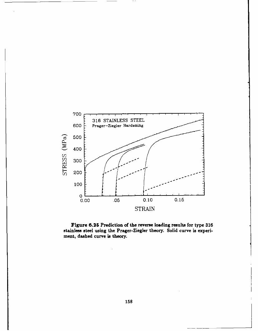
700316 STAINLESS STEEL

600 Prager-Ziegler Hardening

O 500

-400

u3 300

o 200

100

00.00 .05 0.10 0.15

STRAIN

Figure 6.25 Prediction of the reverse loading results for type 316stainless steel using the Prager-Ziegler theory. Solid curve is experi-ment, dashed curve is theory.

158

8 0 0 . . . l . . I . . . I ..

STAINLESS STEEL

700 KIEG MODEL, 9 =0.88

• , 600

500

c 400

300

V' 200

100

00.00 .05 0.10 0.15 0.20

STRAIN

Figure 6.26 Match of reverse loading test using the Krieg theorywith = 0.88. Solid curve is experiment, dashed curve is theory.

159

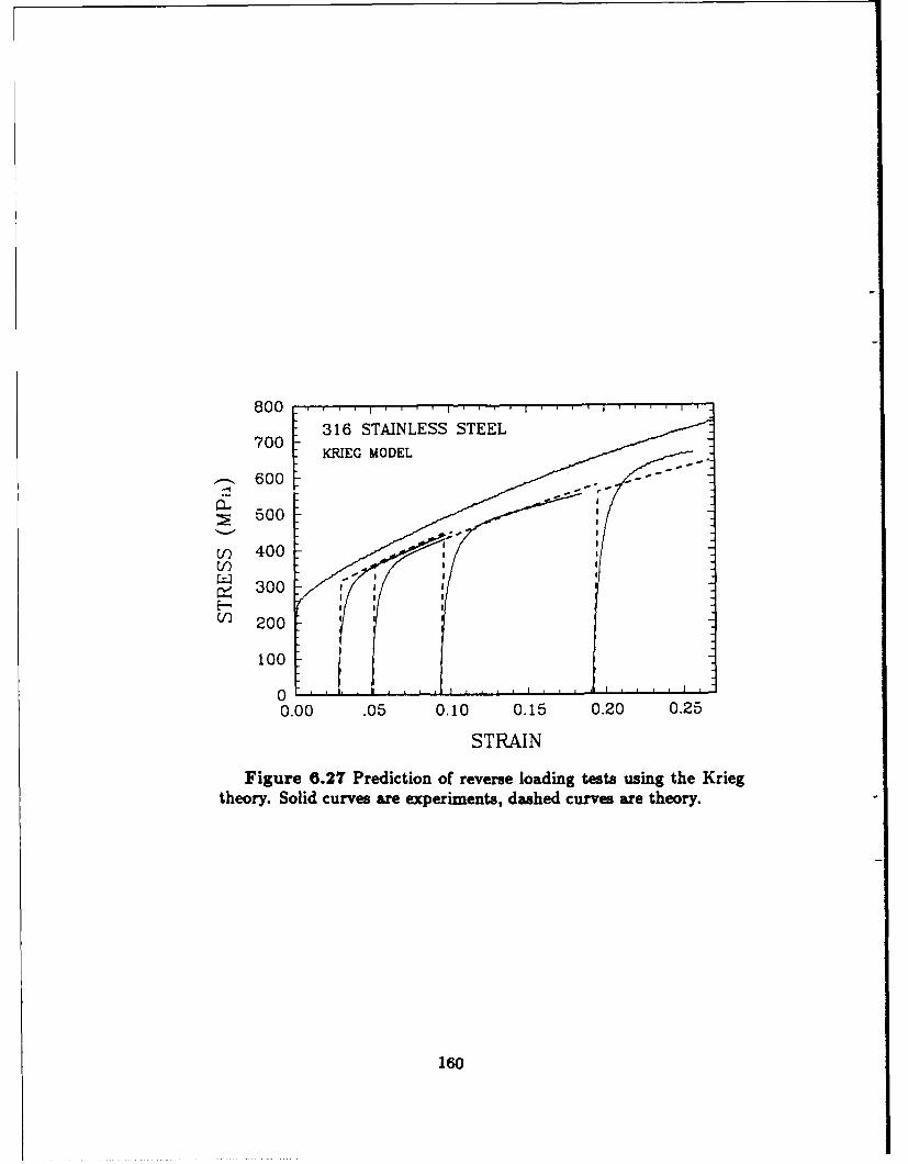
316 STAINLESS STEEL700600 . KRIEG MODEL

500 "

v) 400

~ 300 a

U' 200

100

00.00 .05 0.10 0.15 0.20 0.25

STRAIN

Figure 6.27 Prediction of reverse loading tests using the Krieg

theory. Solid curves are experiments, dashed curves are theory.

160

1500 316 STAINLESS STEEL

1000

S 500

---------------

~-----------------1000

-1500-.06 -. 04 -. 02 0.00 .02 .04 .06

STRAIN

Figure 6.28 Prediction of cyclic test using the Krieg theory. Solidcurve is experiment, dashed curve is theory.

161

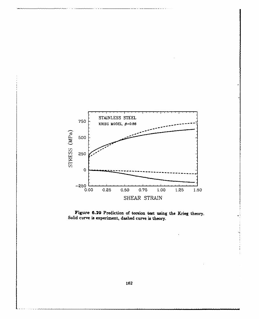
STAINLESS STEEL?50KRIEG MODEL, 9=O.88

500

250

0

-250 L . .'. . . . . . . .'. .

0.00 0.25 0.50 0.75 1.00 1.25 1.50

SHEAR STRAIN

Figure 6.29 Prediction of torsion test using the Krieg theory.Solid curve is experiment, dashed curve is theory.

162

60 316 STAINLESS STEEL- -

- 500

400

U)300

E-200

100

00.00 .05 0.10 0.15

STRAIN

Figure 6.30 Prediction of the reverse loading tests using the Mroz

[19671 model. Solid curves are experiments, dashed curves are theory.

163

Chapter 7

Comparison of Theory withExperiments

In this chapter the theoretical framework developed in Chapter 5 is applied to the

experiments of Chapter 6. Simple material functions are chosen for the materials

studied. The correlation that these give with the basic experiments as well as pre-

dictions of the more complicated experiments are presented. The specific functions

presented are not intended to be final, general forms applicable to all materials.

Rather, simple forms are chosen which are consistent with the criterion given in

Section 5.4.

7.1 Specific Material Functions Employed

Referring to the equations 5.1-5.4 and eqs. 5.9 and 5.10, we note the need to

postulate material functions for 77,CI, C 2, hl, and h2. In Chapter 5 it was shown

that C, and h2 could be functions of {s, g, B,,..} where g and B,,,.. were defined

as the fractional distance transversed of the maximal back stress surface and the

size of that surface. C2 will be considered a constant and h, a function only of 8.

The plastic spin coefficient, Y7, is also considered a constant. These dependencies

164

are summarized as:

C, = 61(s, gB,,z),

C2 = constant,

hi =

h, = hi(s,

77 = constant.

The plastic hardening modulus, H, was determined from the consistency condi-

tion (Equation 5.8).

A universal form was employed for hi(s) for all of the materials investigated:

hi(s) = h1 o(1 - (7.1)

This material function has proven effective in modeling stress-strain results hav-

ing a stress saturation [Brown, 1987] and also those without a measurable saturation

state [Bronkhorst, 1988]. This function has three parameters hi0 , ., and q. The

value of a* determines the saturation level, q controls how quickly that is reached,

and h10 sets the hardening level. A material that shows no saturation in the strain

range of interest is modeled by choosing s" and q such that the predicted satura-

tion is well outside of the working range. Linear isotropic hardening is achieved by

setting s* to a very large value or by setting q to zero.

In choosing a function for k 2(a, g, Bm) it is necessary to satisfy the conditions:

k2 -+ 0 as a --+ s. (a. is the annealed value of a), /2 increases monotonically with

both s and B,..., and h2 -+ 0 as g --+ 1 (the back stress has fully reversed in 1-D).

A simple function that satisfies these conditions is

165

h 2 (sg,B..) = h2 B,., (s - a,,) (1 - g). (7.2)

This function has a linear dependence on each of the variables and one coefficient,

h20 , which is used to match the experiments. This particular function, although

quite simple, was used for all of the materials investigated in this study.

The remaining constitutive function is the back stress coefficient C,(a, g, B,,az).

For monotonic loading C1 should be constant so that standard evanescent hardening

is recovered. During reversing there should be a coupling between C1 and h2. This

is expected if it is the same mechanism responsible both for the isotropic softening

and the back stress hardening. Also C1 is expected to increase with B,, ,. The

simple form chosen for C1 is

C =C 1 o + K B,,a,(1 - g) + -h 2. (7.3)3

It was necessary to include the h2 term in C, to ensure that during uniaxial,

reverse flow the tangent modulus is continuously decreasing. This function contains

one reverse hardening coefficient, K, as well as the back stress constant C,0 .

The evolution equations containing the particular constitutive functions used

in this study are presented below. Note that these particular functions are not

presented as the universal functions, rather they are simple expressions consistent

with the constitutive restrictions outlined above.

= {Cl0 + KBa..(1 - g) + 2 ,} DP - CEPB, (7.4)3

h1 (I - hoB..(, - .o)(1 - g)C'. (7.5)

The constants needed to completely specify the material are: Co, K, C2, hio, s', q, h20 ,

the annealed value of s, (a.), and the spin factor, v7.

166

7.2 Simple Example of Model Components

Before applying the evolution equations developed in Section 7.1 (eqs. 7.4 and 7.5)

to the experiments let us first examine the behavior of the model for a single re-

versing event. This proves very illustrative for visualizing the effects of the different

parts of the model.

Figure 7.1 shows the stress-strain response for uniaxial loading in tension fol-

lowed by compression. The stress response is given by the solid line. The stress is

given by the sum of the isotropic and kinematic (back stress) components.

3BT11 = -B 11 ± .

2

Here we are only examining one stress component. The plus sign applies during

tensile straining and the negative sign during compressive strain increments. igure

7.1 also plots these components of the total stress. The back stress initially rises

to saturation during forward straining. Upon reversal it quickly changes sign and

saturates in reverse at the same magnitude. The isotropic component starts at its

initial value and increases monotonically during forward loading. Here the harden-

ing is shown as linear, q = 0. Upon reversal the magnitude of s initially decreases.

Once B 11 has fully reversed then s again shows the same rate of growth as before

reversal.

In Figure 7.1 the effects of the different model parameters are shown. The

constants C10 and C2 control the back stress growth during monotonic loading. C10

gives the initial slope and the ratio -" gives the saturation magnitude. During

reversing, it is primarily the value of K that determines how quickly B 11 reverses.

K controls the sharpness of the reversing knee of the back stress evolution curve.

167

The isotropic softening variable, h20 , primarily controls the decrease in s imme-

diately after reversing the direction of loading. It influences the permanent softening

but not the stress response immediately after yield due to the presence of the h2

term in C1.

The influence that the constants CI0 , C2 , K, h10 , and h20 have on the stress-

strain response can be seen from Figure 7.1 since the stress response is a sum of

the isotropic and kinematic components. The next section will consider how these

parameters are chosen.

7.3 Procedure for Determining Constants

Whenever a theory is considered for a particular application care must be taken to

prescribe how the theory will be fit to that material and range of strain rate and

temperature. A rational method for determining the material parameters must be

chosen or the theory is of no practical use. The experiments that are required need

to be clearly specified.

In this section a methodology for determining the material parameters is given

and applied to the materials under consideration. The experiments that were re-

quired to completely specify the constants consisted of the uniaxial monotonic (ten-

sion or compression) test, the uniaxial single reverse tests, and the large strain tor-

sion test. The material model was completely specified by these tests. They are

the model construction tests. The cyclic and nonproportional tests are the model

verification tests and are used only to investigate the predictive capability of the

model.

The strategy used to determine the material parameters is as follows. The

168

back stress constants C10 and C2 are determined from the reversing experiments by

looking at the reverse yields. Once they are known the back stress evolution under

monotonic loading can be predicted. The tension or compression test is then used

to find the constants in h1 . For monotonic radial loading the back stress is known.

Its contribution to the total stress can be subtracted out leaving just the isotropic

variable. For monotonic loading h2 = 0 so the function h can be fit to the isotropic

variable evolution.

The transient reverse hardening and isotropic softening are both manifested in

the reverse loading tests. The values of K and h20 are chosen to match to the

reversing portions of the tests. The value of K controls the sharpness of the knee

of the reverse loading curve and h20 controls the permanent softening.

From these tests the proper effects can be isolated to determine the material

constants. From the strategy outlined above, the following methodology was used

to select the parameters of the model for the materials considered in this study.

1. Determine the back stress evolution from the reverse loading tests.

From the stress-strain results for reverse loading find the reverse yield stress

ar. This is determined using a certain offset definition for the reverse yield.

This offset is in the approximate range of 0.05% to 0.3% strain. The tensile

equivalent back stress is then determined as ab = 1(o! + cr) where a is the

forward flow stress achieved before reversing. Note that a, can be positive or

negative in sign. Since the back stress tensor B is deviatoric (trB = 0) the

component in the direction of loading of the experiment is

Bil = 2 1 (o! + a,). (7.6)3 3

169

The constants CI0 and C2 are chosen from the evolution of B1 with plastic

strain clIP.

B11 (7.7)C2

The ratio - is chosen to match the saturation value of B11 achieved at large

C2

strain. The value of C2 is then chosen to match the time constant or rise time

of the results.

This procedure gives a systematic manner of selecting C10 and C2. Figure 7.2

shows this fitting for type 316 stainless steel.

2. Determine the isotropic hardening constants. From equation 7.7 the

back stress evolution for uniaxial, monotonic loading can be predicted. The

evolution of the isotropic variable s for monotonic loading is found by subtract-

ing the back stress from the total stress. For each point on the stress-strain

curve the value of s is given by

3B

s = u--B 11, (7.8)2

where B11 is given by equation 7.7. This is illustrated in Figure 7.3 for the

compression of type 316 stainless steel. Once the curve of 8 versus plastic

strain is known the material constants can be fit. For monotonic loading

h2 = 0 so:

i = hio (1 - ) " (7.9)

is the functional form to be fit. Integration of equation 7.9 [Brown, 1987]

yields

170

s = _ (a - 8 )(I - ) + (q - 1){hlo(a')- IT ' , (7.10)

where a. is the initial value of a and h10, ", and q are the material parameters.

This function has four parameters. Theoretically they could all be determined

using a four parameter least squares fit. In practice, . and 8" correspond to

the initial and saturation values of s so they can be chosen or inferred by

extrapolation from the results of a versus plastic strain. Nonlinear fitting for

h10 and q was performed with an IMSL numerical subroutine ZXSSQ which

provides for minimization of a nonlinear function on the basis of a least squares

residue. For type 316 s.s. in compression this fit is shown in Figure 7.4.

This procedure yields consistent values of the parameters and provides a check

on the choice of offset reverse yield definition. We make the assumption that,

for monotonic loading from the annealed state, the value of a should also

increase monotonically. If too small of an offset yield definition is used this

does not hold. The inferred curve of s versus plastic strain then shows an initial

dip. This is not consistent with the initial annealed state of the materials

tested in this study. We expect that a should show a monotonic increase with

plastic strain. Choice of reverse yield defined by a 0.05% to 0.3% offset strain

satisfies this requirement.

3. Determine the Reversing Coefficient K and the Isotropic Softening

Coefficient h20 . Using the previously determined values of C10 , C2 , hi 0, ,go,

and q the reverse loading experiments are simulated with different values of K

and h20. To select the appropriate values, first set h20 = 0 then simulate one

of the reverse loading tests for various values of K. The test to be matched

171

should be one which has the back stress well developed (,Ef -- 0.1). The

simulation will have no permanent softening for h20 = 0 but choice of K

should be made to match the initial steeply rising portion of the reversing

curve.

Once the order of magnitude of K is known then isotropic softening is added

by increasing h20. This will be seen as an increase in permanent softening.

As h20 is changed, K will also need to be changed to provide good agreement

with the rising portion of the reverse curve. There is a coupling of the effect

of h 20 and K on the reverse flow curve. In a few trials K and h20 can be

selected to give good agreement.

When K and h20 have been selected from the one reverse test they should

next be used in simulating all of the reverse tests. If good agreement is not

obtained for all of the tests then different functional forms are needed for h2

and C1. These can be modified and new values for the coefficients selected

using the same procedure.

The procedure which has been described in this section uses just two types of

experiments (uniaxial monotonic and single reverse) to select all of the material

parameters of the proposed combined kinematic-isotropic model.

Table 7.1 Material Constants

material CI0 C2 h10 q so a* K h201100 alum (t) 500 25 39,619 13.619 47. 200 600 101100 alum (c) 500 25 276 1.015 53 150 600 10316 s.s. (t) 1780 17.8 1600 0.3189 240 1100 200 1.5316 s.s. (c) 1780 17.8 1752 0.3345 290 1200 200 1.51020 5233.3 50 19,256 7.7106 175 1217 150 11045 5600 40 8255 5.361 350 1414 150 31095 6934 40 39,825 5.249 442 1000 100 10

172

The one remaining parameter, the plastic spin factor, is considered by examining

the large strain torsion response. Calculations of the model for different values of 17

are directly compared with the experimental shear stress and normal stress response.

The question of the importance of plastic spin can be addressed by this approach.

If it is important, the choice of q from this matching completes the model. If it

does not matter, or it the value of 17 =0 provides the best match to the experiment,

then plastic spin is not important for this application.

7.4 Correlation of Theory with Base Experiments

In section 7.3 the procedure for choosing the constants in the theory was discussed.

Appropriate values for the coefficients were chosen from the set of base experiments.

In this section the comparisons of the theory with these tests are presented. These

results do not show the predictive capability of the model but rather how well it

correlates the tests. In section 7.5 the predictive capabilities will be examined.

These experiments used for model construction include tension, large strain

compression, and single reverse tests for the following materials: type 316 stainless

steel, 1100-0 aluminum, and three spherodized carbon steels (1020, 1045, 1095).

The carbon steel data are from the studies of Bronkhorst [19881.

The reversing tests were used to determine the back stress evolution during

monotonic loading. The constants C10 and C2 were used to predict this growth.

Figure 7.5 shows the correlation of the model with the experimentally inferred data

points. Notice that the theory predicts a saturating, decaying exponential behavior.

C10 .B1 =-- -( (1 - ec-2P). (7.11)

C2

The experimental back stresses were determined using various percent offset def-

173

initions for reverse yield, as discussed in section 7.3. The offsets that were used

were: 0.3% for type 316 s.s., 0.05% for 1100-0 aluminum , 0.3% for 1020, 1045,

1095 carbon steel. These offsets were chosen to ensure a monotonically increasing

isotropic component during forward loading as discussed above.

After the back stress evolution was chosen, the isotropic component was fit and

the tension and compression curves were simulated. These are shown in Figures 7.6

to 7.12. The simulation of these results is very close as expected.

The reverse loading experiments were also used to select the level of isotropic

softening and additional back stress stiffening. The correlation of these experiments

with the model is shown in Figures 7.13 to 7.17. The proper trends are captured

by the model for each material. The initial high stiffening during reversing is well

matched. The permanent softening trends are also well represented. Better corre-

lation could be obtained if different functions for 4 and di were chosen for each

material. The ones that were chosen were intended to be simple, having few param-

eters, yet retaining the proper constitutive restrictions. In that light the correlation

is quite good.

This section has presented the comparisons of the model with the base experi-

ments used to determine the evolution equations. The correlation is quite satisfac-

tory as five materials are modeled with the same simple constitutive forms.

7.5 Evaluation of the Predictive Capability of theModel

The true test of a constitutive model comes not from its accuracy in modeling the

tests that were used to construct the model. Rather, a model should be evaluated

according to its ability to predict the behavior of different types of experiments. In

174

this section, the proposed constitutive model is used to predict the response under

different types of loading than were experienced in Section 7.4.

The tests that were predicted were:

Symmetric, strain-controlled, cyclic tests of 316 s.s. and the carbon steels.

Unsymmetric, strain-controlled, cyclic tests of the carbon steels.

Unsymmetric, stress-controlled, cyclic test of 1045 carbon steel.

90 out-of phase strain-controlled cyclic test of 316 s.s.

Large strain, fixed end, torsion tests of 316 s.s. and 1100-0 aluminum.

Using the material parameters determined in the base experiments described in

Section 7.4, the experimental data and model predictions are compared. For each

test it is the stress response that is examined.

7.5.1 Symmetric Strain Cycling

The model has been derived from mainly monotonic type loading. The single reverse

experiments were used but not cyclic tests. A type of experiment that is a good test

for the model is symmetric strain cycling. This test is important because it can be

cycled to achieve a stable, saturation loop. If a model does not do a closely match

the state after one reversal then the errors are accentuated with many cycles. In

Figures 7.18 to 7.21 the experimental results and model predictions are presented

for the symmetric strain cycling of four materials. Notice that the model does a

good job of matching not only the final stress level but also the rate of buildup of

stress. For each of these materials the response was cyclic hardening since they had

175

initially been in the annealed condition. For each test the nominal cycling range

was ±5% strain.

In predicting this behavior the model behaves differently than most of the mod-

els in the literature. During each half cycle the isotropic component initially softens,

then hardens. In the more classical models the isotropic component is always mono-

tonically increasing with strain. At the cyclically stable state, these models predict

that the isotropic component has its maximum saturation value, the value that it

would achieve at large strain in a compression test. The new model predicts that the

stable cycle is reached when the hardening and softening occuring during each half

cycle just balance each other out. The maximum value of the isotropic component

reached in the stable cycle depends upon the strain limits. For a larger hysteresis

loop, a greater amount of hardening takes place and the isotropic component is

larger. This means that for predicting cyclic plasticity, the isotropic component of

stress depends upon the strain limits. This is just what is observed experimentally.

For monotonic loading the isotropic component can reach a much greater value

than for small to moderate strain cyclic plasticity. Modeling this behavior is an

important feature for a general model for the small to large strain regimes.

7.5.2 Unsymmetric Strain Cycling

The symmetric cyclic tests give cyclic hardening. The results of Bronkhorst [1988]

include unsymmetric strain cycling tests which show cyclic softening and mean stress

relaxation for the three carbon steels. In Figures 7.22 to 7.24 the experiments and

predictions are compared. For all three materials the tests consisted of a forward

prestrain to approximately 9% strain followed by strain controlled cycling between

7% and 9% strain. The tests show cyclic softening as the hysteresis loops get

176

continuously smaller with cycling and approach a stable loop. The loops shrink

mainly by a reduction in stress of the positive loading half cycle. The compression

half cycle maintains the same stress.

The model predicts the stress softening (through the softening of the isotropic

component) and the correct, stable hysteresis loop. What the model does not do

as well is follow each cycle as it gradually softens to the stable state in about 5

cycles. The model achieves the final state in 1 or 2 cycles. This is not a major

shortcoming. The characteristic features of this test are well predicted. The size of

the stable loop is largely set by the value of s, for cyclic softening conditions. The

back stress merely alternates but s decreases. The factor (s - so,) in 1 2 is necessary

to prevent s from softening below its annealed value. Figures 7.22 to 7.24 show that

physically this is what limits the softening.

For the 316 s.s. an unsymmetric strain cycling test was conducted that consisted

of forward loading to a strain of 19%, reverse straining to 17%, then forward strain-

ing. Figure 7.25 shows the prediction of the theory against the experiment. The

model does an adequate job predicting the response here as with the unsymmetric

strain cycling of the carbon steels.

7.5.3 Unsymmetric Stress Cycling

The experiments of Bronkhorst [1988] include unsymmetric stress cycling results

of the carbon steels. Here we predict the behavior for the case of unsyimmetric

cycling of 1045 carbon steel. The specimen was cycled between stress limits of

+490 Mpa in tension and -430 Mpa in compression. The results of both simulation

and experiment are shown in Figure 7.26.

The model correctly reproduces the hysteresis loop seen in the experiment. The

177

correct width and shape are predicted. The model does not do as well predicting

the actual amount of cyclic creep. After 41 cycles the experiment has accumulated

about 4% plastic strain but the model predicts about 51% accumulated plastic

strain. When considering how other models do at predicting cyclic creep this is quite

reasonable. The model does not do better due to the very low tangent modulus

to the stress-strain curve at this level of strain. A small discrepancy is the stress

prediction is magnified by the strain response. Overall, the model captures the

correct behavior.

7.5.4 900 Out-of-Phase Cycling

The predictions of the two types of tests described above very heavily activate the

isotropic softening function h2 but do not test the tensorial nature of the constitutive

equations since they involve uniaxial loading. One of the types of experiments that

is not so limited involves cycling in the tension-torsion subspace. This involves

radial loading in either the tension or shear direction to . certain prestrain then

cycling by following a circular trajectory in strain space keeping the equivalent strain

constant. These types of experiments have been cited frequently in the literature as

a basic test of nonproportional, cyclic, plasticity [Lamba and Sidebottom, 1978b],

fCailletaud, et al., 1984]. The experiments of Cailletaud et al. [19841 were for

type 316 stainless steel. Although this material was heat treat,:d differently than

the annealed type 316 tested in this study, a simulation was conducted using the

material constants developed here.

Figures 7.27a and b show the experimental results of Cailletaud and a simula-

tion of this test with the current model. Notice that the sane features are observed

for both: a spiraling outward stress trajectory that saturates. The level of this

178

saturation stress value is higher than the corresponding saturation stress for uni-

axial cycling at the same maximum strain range. The experimental results shown

in Figure 7.27a are for a total imposed strain range of ±1.5%. The out-of-phase

stablization stress is 800 MPa. This compares with 550 MPa for the uniaxial sta-

bilization stress for the same maximum strain cycling range. The simulation of

Figure 7.27b predicts a stablization stress of 1105 Mpa. This compares with a

model prediction of the uniaxial stablization stress of 496. Mpa. Notice that the

additional hardening which is seen experimentally is picked up by the model. This

is a natural consequence of the physics of isotropic recovery limiting the uniazial

stress but not the out-of-phase cycttng. The other models which attempt to model

this well known behavior do so by increasing the isotropic hardening modulus or

making the isotropic saturation value depend upon some measure of nonpropor-

tionally [McDowell, 1987], [Benallel and Marquis, 1987], [Lindholm et al., 1985]. In

the model presented here, additional hardening is a natural consequence except it

is a misnomer to call it additional hardening. Really, it is the uniaxial cycling tests

that show reduced hardening.

For uniaxial, symmetric cycling it was observed that the stabilization stress

depended upon the competition between h, and h2. For out-of-phase cycling, the

back stress remains on its maximal surface during all of the deformation except

right after the initial strain corner going from preloading to cycling. Thus s is not

limited by softening and increases to its saturation value of s'. So s" is the important

parameter determining the saturation stress level. There are important differences

between uniaxial and out-of-phase cycling but the new constitutive model is able

to predict them well.

179

7.5.5 Fixed End Torsion Tests

The deformation mode with the biggest interest in recent years has been simple

shear. This deformation not only involves nonproportional loading but also material

rotation at large deformation. The fixed end, torsion test of thin-walled tubular

material provides the best experimental measure of simple shear.

Figure 7.28 presents the composite results of the 316 stainless steel torsion test.

Both shear and normal (axial' stresses are shown as a function of engineering shear

strain. The predictions of the model for simple shear are also displayed. For all of

the torsion test predictions, the material constants reduced from the compression

tests were used. This gave slightly different isotropic hardening parameters than

if the tensile curve was used but more reliable large strain predictions since less

extrapolation was required. The predictions in Figures 7.28 and 7.29 have 17 = 0,

no plastic spin.

Notice that even without using plastic spin, the predicted stresses do not show

any oscillations or inflections. The predicted normal stresses are also quite small,

much smaller than those that were observed. Both of these result from the evanes-

cent back stress evolution law. The value of C2 , the evanescent term, determines

the importance of the evanescent or damping term. When C 2 is chosen large enough

to properly model the back stress growth during uniaxial loading it does not allow

for much buildup of normal stress during simple shear. The axial normal stress

monotonically increases to a saturation value which, for small elastic strain and

C 2 >> 1 yields,

at 1 T122 3 C,T22"' = __+ -2 tz 2 C2

ThLe first term gives the elastic contribution and the second gives the plastic con-

180

tribution to the normal stress. For realistic values of C 2 (15-50) the plastic term is

quite small and for metal plasticity the elastic term is also quite small. Substantial

normal stresses are not predicted using the evanescent evolution law.

The effect of r/ is unimportant with these material constants. The effect that

P7 has on the stress response is to decrease the magnitude of the normal stress and

increase the shear stress. That would lead to slightly worse results here. For an

evanescent law with realistic choices of C, and C2 the plastic spin is unimportant.

The new model does not predict an oscillatory sterss response even without acti-

vating the plastic spin.

The comparison of the shear stress result is not much better than the normal

stress. The shear stress does not harden nearly as much in the experiment as the

theory predicts.

These same trends are seen in Figure 7.29 for the torsion test of 1100-0 alu-

minum. Here the experimental normal stresses are smaller in relative magnitude

than for the 316 s.s. but are still well underpredicted by the theory. The shear

stress prediction is also higher than the experiment.

Figure 7.30 shows the simple shear prediction of 1100-0 aluminum carried out

to ve.-y large shear strain (500%). Notice that for the realistic choice of material

constants that no stress oscillation is seen. The shear stress approaches an asymp-

totic value. It is not necessary to include plastic spin to have monotonic stress

response.

The proposed constitutive model works well for the cyclic tests (both propor-

tional and nonproportional) but not as well for the large strain torsion test. The

evanescent nature of the back stress evolution equation captures the cyclic response.

181

Even the out-of-phaze tension-torsion cycling shape is well represented. In fact, the

C2 term in the evolution equation is necessary to center the stress hysteresis spiral

on the stress origin. The often debated question of the importance of plastic spin

becomes moot for an evanescent back stress law with realistic constants.

182

REVERSING BEHAVIOR750 New Modell

500 __.s.........

250

"-" ... .... C,o/C2Vl) 0 .WCIo/C2 ,Ix - ------------------

E- B1 ,

) -250

-500

T1,

-750

, p , I p p p I , p I p I p I I

0.00 .02 .04 .06 .08 0.10

PLASTIC STRAIN

Figure 7.1 Schematic diagram of the new constitutive model sim-ulating a uniaxial, single reversing test. The back stress componentB11, the isotropic component s, and the total stress T, are shownto illustrate their behavior. The reversing coefficient K affects thesharpness of the knee of the B1, response immediately after strainreversal. The isotropic softening coefficient h20 affects the softeningof the s response curve immediately strain reversal.

183

316 STAINLESS STEELE-- Back Stress Evolution0

z 100

~- 75

0U

Cl) 50

E- 25

II

U00.00 .05 0.10 0.15 0.20

PLASTIC STRAIN

Figure 7.2 Comparison of experimentally determined back stress

with fit. Cl0 = 1780., C2 = 17.8.

184

1250 316 STAINLESS STEELCompression

1000

750

S 500

CTr

250

Back Stress B,1

0 . . - ....

0.00 0.10 0.20 0.30 0.40 0.50 0.60 0.70

STRAIN

Figure 7.3 Decomposticn of uniaxial stress-strain by subtractingback stress component from total stress to determine isotropic a.

185

1200 316 STAINLESS STEELCompression Test

1000

800C/9/ s= 1200

0 600 hlo=1752-Q) 40 q=0.3345

S 400

200

0 I i i i .i 1 [ i i

0.0 0.1 0.2 0.3 0.4 0.5 0.6 0.7

PLASTIC STRAIN

Figure 7.4 Fit of isotropic hardening function to inferred curveof a. Solid curve is experiment, dashed curve is fit.

186

1 4 12 ,5 . . .-. . . . , . .

316 STAINLESS STEEL

E-- Back Stress Evolution 0Z 100

0C- 75

500Cl) 50Cl)

E-- 25

0.00 .05 0.10 0.15 0.20

PLASTIC STRAIN

Figure 7.5a Back stress evolution for type'316 stainless steel.

187

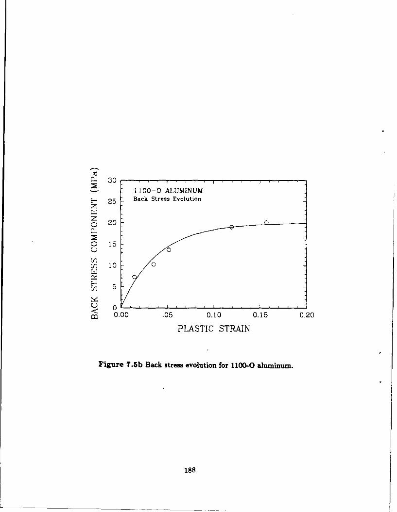
30

1100-0 ALUMINUME- 25 Back Stress Evolutionz

0 20

0 15

10 10

5

0 .. . . t . . .. .. ..

0.00 .05 0.10 0.15 0.20

PLASTIC STRAIN

Figure 7.5b Back stress evolution for 1100-0 aluminum.

188

1000 1 1 1 1

316 STAINLESS STEELTensile Test Simulation

800

S 600

S 400

200

0.00 .05 0. 10 0.15 0.20 0.25 0.30 0.35 0.40

STRAIN

Figure 7.6 Comparison of tensile test with model fitting for type316 stainless steel. Solid curve is experiment, dashed curve is model.

189

150

1100-0 ALUMINUM

125 TENSION TEST COMPARISON

S100

-n 75

50

25

0.00 .05 0.10 0.15 0.20

STRAIN

Figure 7.7 Comparison of tensile test with model fitting for 1100-(~aluminum. Solid curve is experiment, dashed curve is model.

190

700 1 1 T I

1020 CARBON STEEL600 Tensile Test Simulation500 ,, ,

U 400

S300

200

100

0.00 .05 0.10 0.15 020

STRAIN

Figure 7.8 Comparison of tensile test with model fitting for 1020carbon steel. Solid curve is experiment, dashed curve is model.

191

900

1045 CARBON STEEL8O00

Tensile Test Simulation7100

600500

k-400

300

200

100

00.00 .05 0.10 0.15 0.20

STRAIN

Figure 7.9 Comparison of tensile test with model fitting for 1045carbon steel. Solid curve is experiment, dashed curve is model.

192

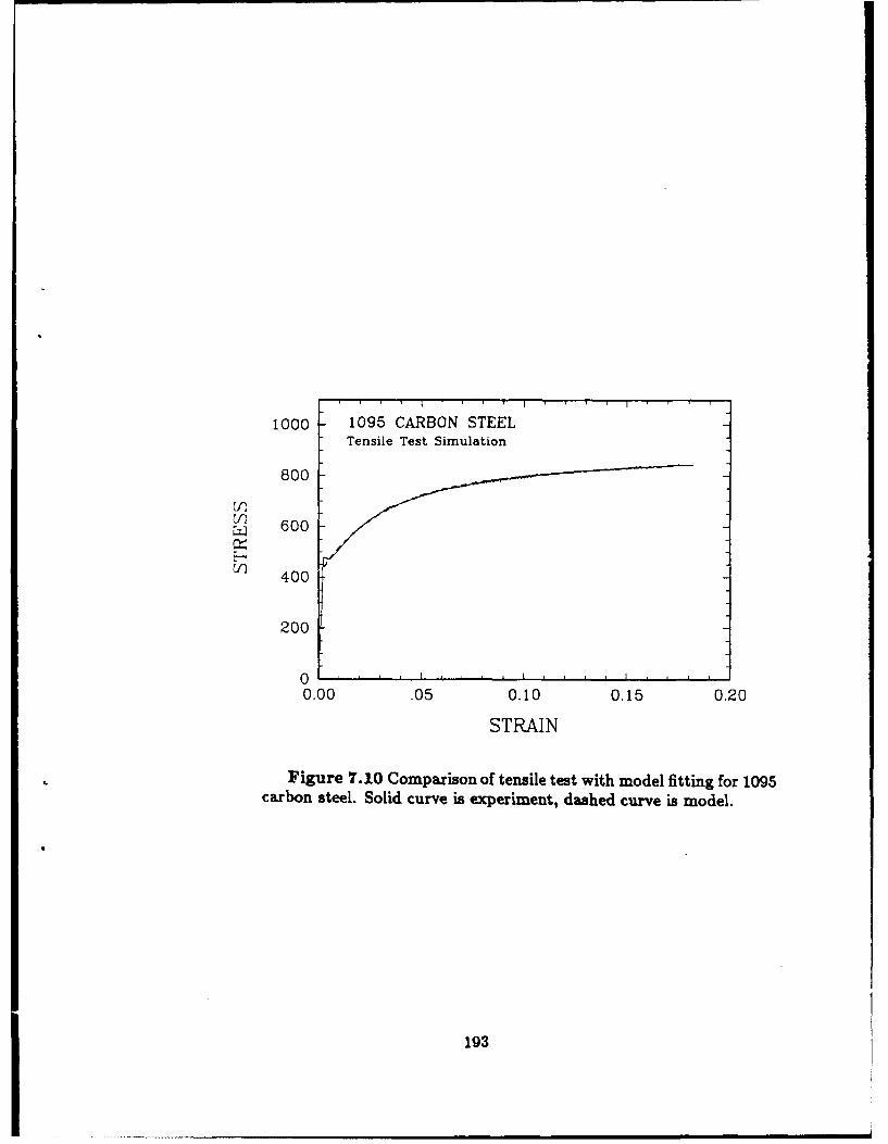
1000 1095 CARBON STEELTensile Test Simulation

800

S 600

400

200

0.00 .05 0.10 0.15 0.20

STRAIN

Figure 7.10 Comparison of tensile test with model fitting for 1095carbon steel. Solid curve is experiment, dashed curve is model.

193

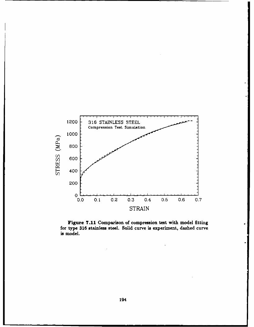
1200 316 STAINLESS STEELCompression Test Simulation

~_~ 1000

~ 800

) 600

E- 400

200

O I I .1,, i I ,

0.0 0.1 0.2 0.3 0.4 0.5 0.6 0.7

STRAIN

Figure 7.11 Comparison of compression test with model fittingfor type 316 stainless steel. Solid curve is experiment, dashed curveis model.

194

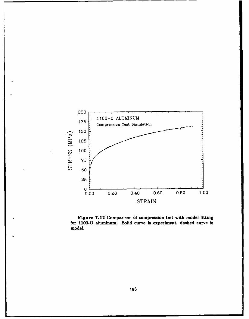
2001100-0 ALUMINUM

175Compression Test Simulation

-~ 150

125

c 100

( 75

50

25

0.00 0.20 0.40 0.60 0.60 1.00

STRAIN

Figure 7.12 Comparison of compression test with model fittingfor 1100-0 aluminum. Solid curve is experiment, dashed curve ismodel.

195

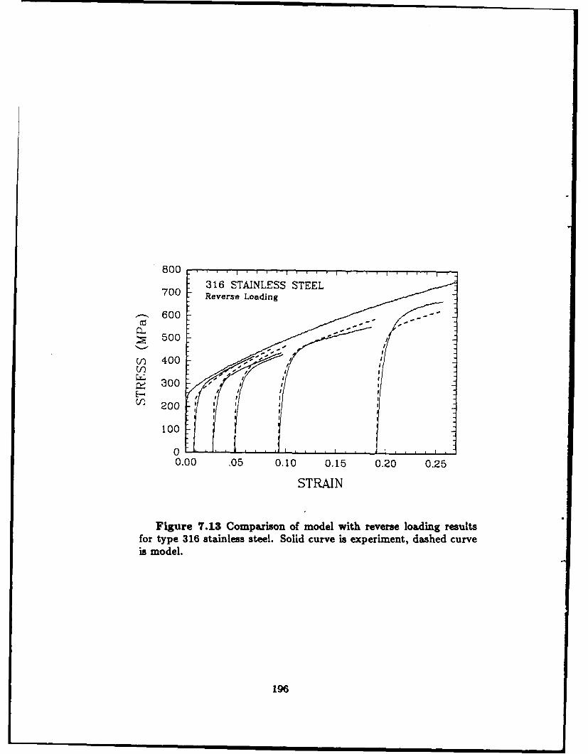
8 0 0 . . i . . . . I . . . . I ,316 STAINLESS STEEL

700 Reverse Loading

-~600

S 0500

--- 400C4 300

100

1000 . .

0.00 .05 0.10 0.15 0.20 0.25

STRAIN

Figure T.13 Comparison of model with reverse loading resultsfor type 316 stainless steel. Solid curve is experiment, dashed curveis model.

196

125

1100-0 ALUMINUMReverse Loading

100

S 50

25

00.00 .05 0.10 0.15 0.20

STRAIN

Figure 7.14 Comparison of model with reverse loading results for1100-0 aluminum. Solid curve is experiment, dashed curve is model.

197

7001020 CARBON STEEL

600 Reverse Loading

500

400

V'300

V) 200

100

00.00 .05 0.10 0.15 0.20 0.25

STRAIN

Figure 7.15 Comparison of model with reverse loading results for1020 carbon steel. Solid curves are experiments, dashed curves aremodel.

198

900 -T

80 1045 CARBON STEEL700

600

500

400

300

200

0

0.00 .05 0.10 0.15 0.20

STRAIN

Figure 7.16 Comparison of model with reverse loading results for1045 carbon steel. Solid curves are experiments, dashed curves aremodel.

199

900 1095 CARBON STEEL

800 Reverse Loading

700

600

400

300

200

100

0

0.00 .05 0.10 0.15 0.20

STRAIN

Figure 7.17 Comparison of model with reverse loading results for1095 carbon steel. Solid curves are experiments, dashed curves aremodel.

200

1000 316 STAINLESS TES50 "etric Strain CYcig

S-2.50

-5006

STRAINFigure 7'.18 Comparison Of model prediction adeprmnaresu ts f r zk5% y am etric strain cy lin g9 of 31 6) stainless steel. So d

curve is experiment dlashed curve is model.Soi

201

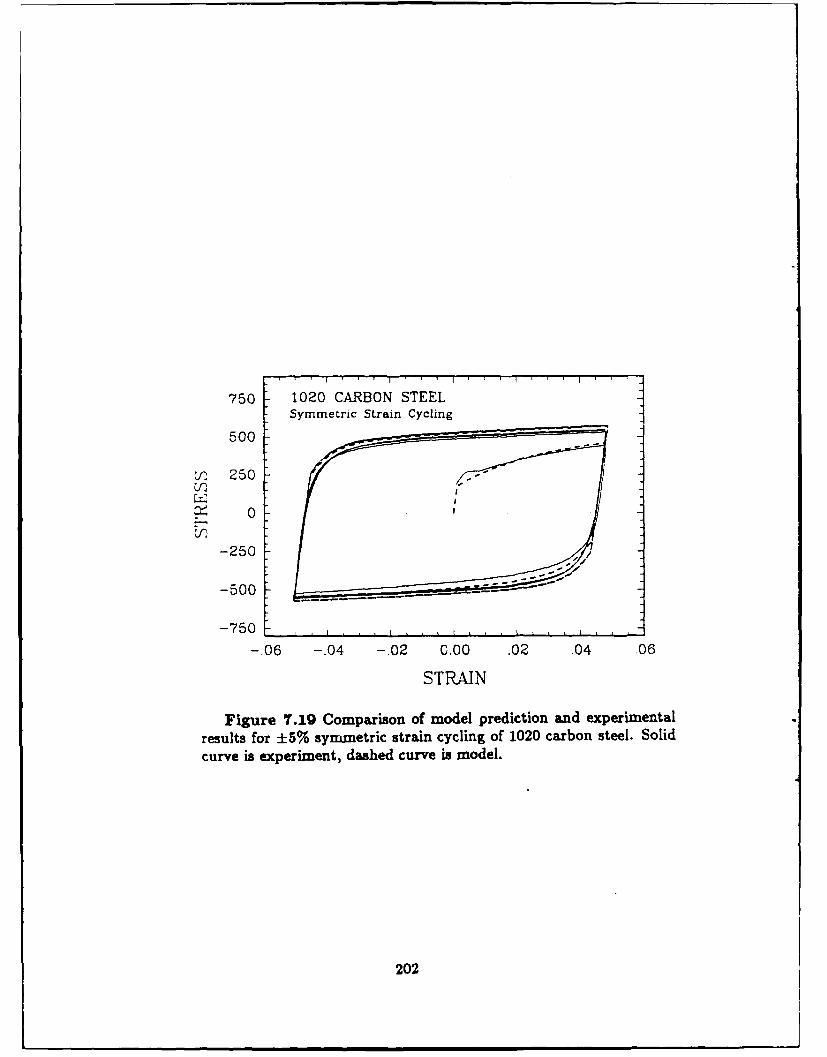
750 1020 CARBON STEELSymmetric Strain Cycling

500

n 250

0

-250

-500 - ---

-750 I I I

-.06 -. 04 -. 02 0.00 .02 .04 .06

STRAIN

Figure 7.19 Comparison of model prediction and experimental

results for ±5% symmetric strain cycling of 1020 carbon steel. Solid

curve is experiment, dashed curve is model.

202

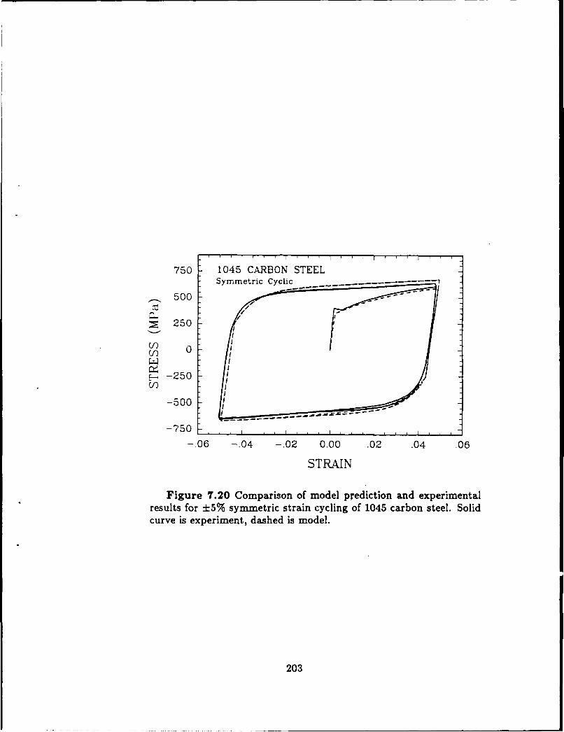
750 1045 CARBON STEEL

Symmetric Cyclic -------

500

-250

-500

-750 I I I I

-06 -. 04 -. 02 0.00 .02 .04 .06

STRAIN

Figure 7.20 Comparison of model prediction and experimentalresults for ±5% symmetric strain cycling of 1045 carbon steel. Solidcurve is experiment, dashed is model.

203

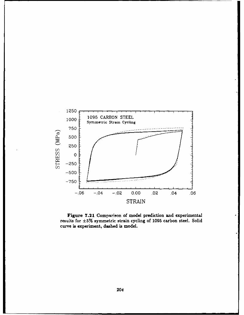
1250

1095 CARBON STEELSymmetric Strain Cycling

7 5 0 -------------------_-

a 500

" 250

0

E- -250

-500

-7 5 0 . .............i I I , i I i i -

-. 06 -. 04 -. 02 0.00 .02 .04 .06

STRAIN

Figure 7.21 Comparison of model prediction and experimentalresults for ±5% symmetric strain cycling of 1095 carbon steel. Solidcurve is experiment, dashed is model.

204

750 1020 CARBON STEELUnsymmetric Strain Cycling

500

250

0

-250

-500

0.00 .02 .04 .06 .08 0.10

STRAIN

Figure 7.22 Comparison of model prediction and experimentalresults for unsymmetric strain cycling of 1020 carbon steel. Solidcurve is experiment, dashed is model.

205

750 1045 CARBON STEELUnsymmetric Cyclic ------- ------

0

2- -250

-500

-750

0.00 .02 .04 .06 .08 0.10

STRAIN

Figure 7.23 Comparison of model prediction and experimentalresults for unsymmetric strain cycling of 1045 carbon steel. Solidcurve is experiment, dashed is model.

206

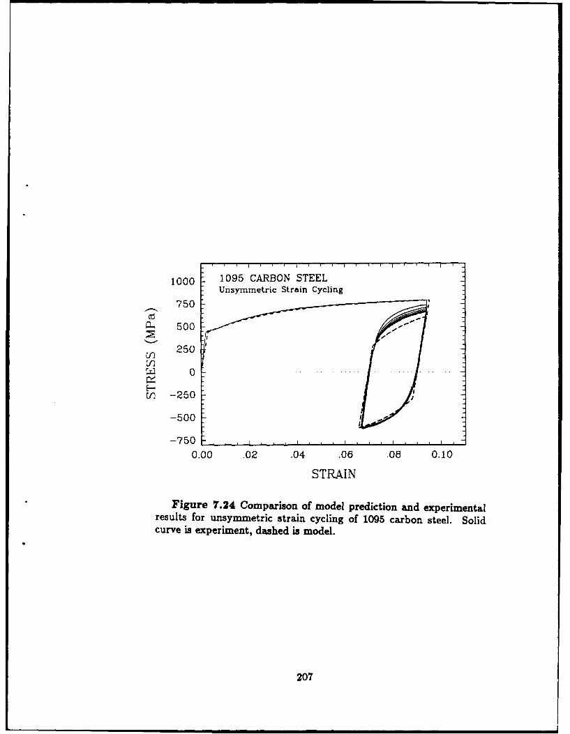
1000 1095 CARBON STEELUnsymmetric Strain Cycling

750~- 500

250

ri -250

-500

-7 5 0 , , . , , , , , , , , , , , , , '

0.00 .02 .04 .06 .08 0.10

STRAIN

Figure 7.24 Comparison of model prediction and experimentalresults for unsymmetric strain cycling of 1095 carbon steel. Solidcurve is experiment, dashed is model.

207

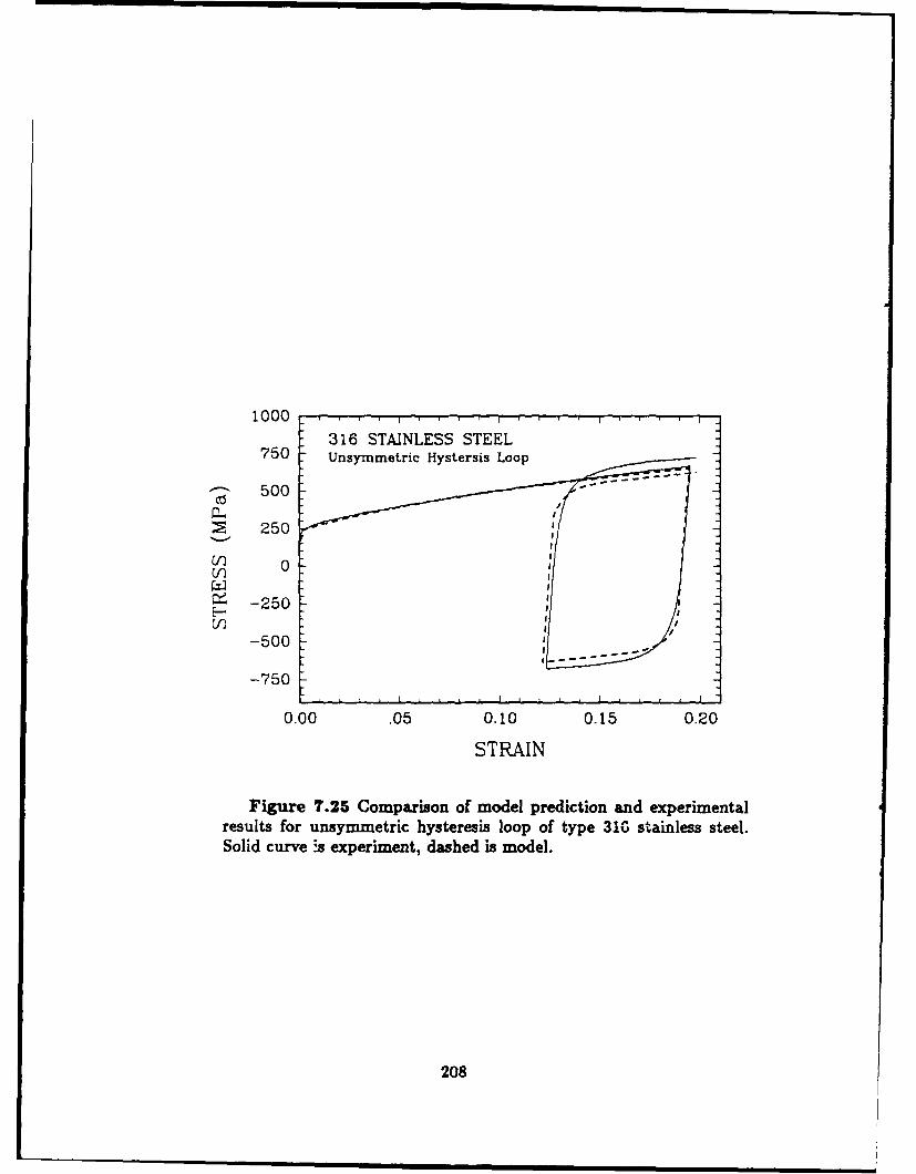
1000

316 STAINLESS STEEL750 Unsymmetric Hystersis Loop

500

~ 250

V) 0

0- -250

-500

-750

0.00 .05 0.10 0.15 0.20

STRAIN

Figure 7.25 Comparison of model prediction and experimentalresults for unsymmetric hysteresis loop of type 310 stainless steel.Solid curve !s experiment, dashed is model.

208

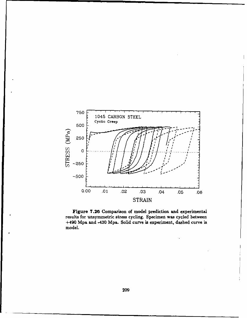
7501045 CARBON STEELCyclic Creep

500

250

) 0 .. ' I;I I/ II -

-250 / .f .r ." ."

-500

0.00 .01 .02 .03 .04 .05 .06

STRAIN

Figure 7.26 Comparison of model prediction and experimentalresults for unsymmetric stress cycling. Specimen was cycled between+490 Mpa and -430 Mpa. Solid curve is experiment, dashed curve ismodel.

209

(a)0

CIS

Axial Stress

316 STAINLESS STEEL-s1000

50

(b) 0

S-500

-1000

-1000 -500 0 500 1000

AXIAL STRESS (MPa)

Figure 7.27 Stress response for 9W out-of-phase tension-torsioncycling of 316 stainless steel. a) Experimental results of Cailletaud etal. [19841. b) Prediction of new model.

210

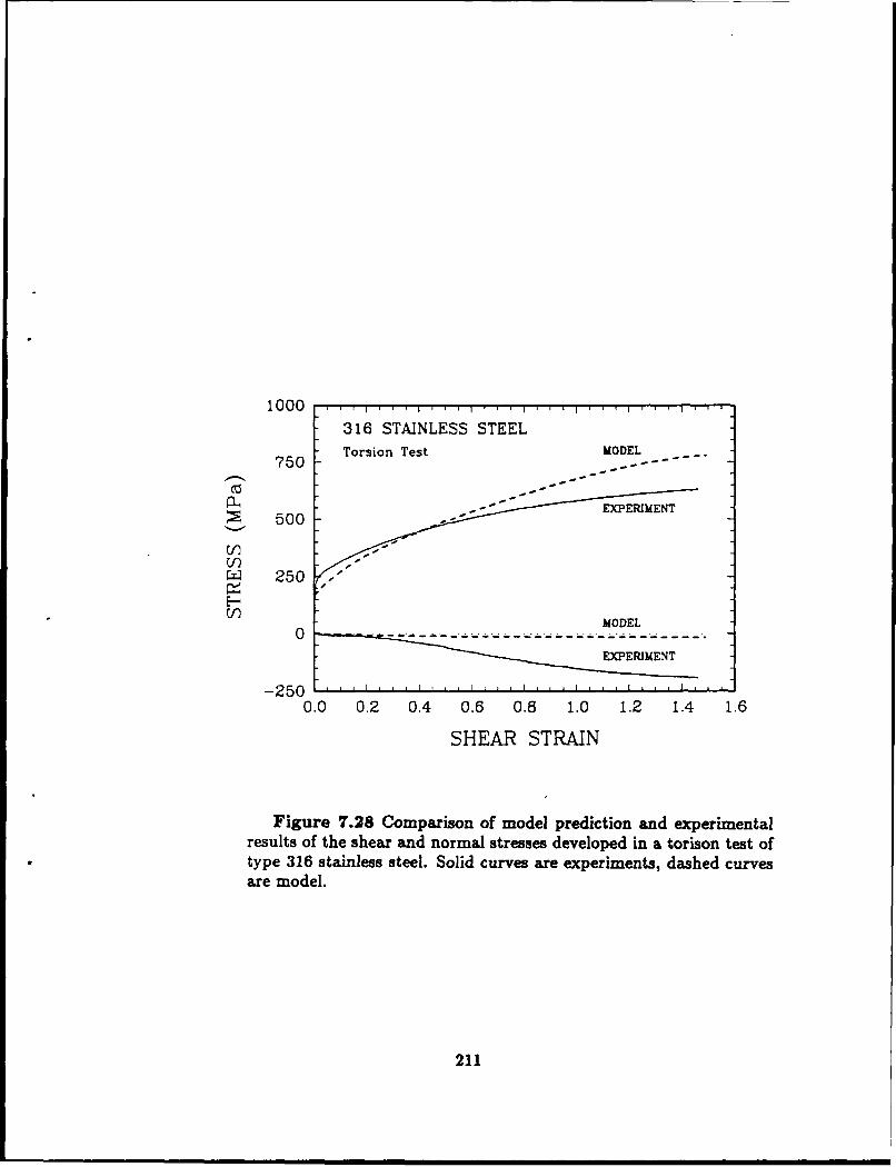
1000316 STAINLESS STEEL

750 Torsion Test MODEL-

500V)

250 .

[.-MODEL

- 250 , , I , , . , , , , . ,

0.0 0.2 0.4 0.6 0.8 1.0 1.2 1.4 1.6

SHEAR STRAIN

Figure 7.28 Comparison of model prediction and experimentalresults of the shear and normal stresses developed in a torison test oftype 316 stainless steel. Solid curves are experiments, dashed curvesare model.

211

100,

1100-0 ALUMINUM

80 Torsion Test

Cl)

60

40V)

• 20

Shear Strain

Figure 7.2g Comparison of model prediction and experimentalresults of the shear and normal stresses developed in a torsion test of1100-0 aluminum. Solid curves are experiments, dashed curves are

model.

212

I0Exeimn

-2 --

0 . . . . . . . . .

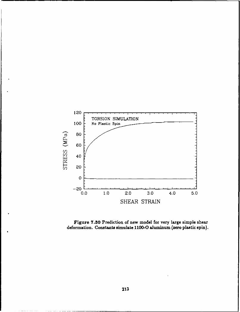
120 T I I

TORSION SIMULATION100 No Plastic Spin

80

60

V) 40

Cn 20

0

-20 L . . . .'. .

0.0 1.0 2.0 3.0 4.0 5.0

SHEAR STRAIN

Figure 7.30 Prediction of new model for very large simple sheardeformation. Constants simulate 1100-0 aluminum (zero plastic spin).

213

Chapter 8

Conclusions

The major results of this study include: fundamental data from critical experi-

ments, crucial observations of material behavior extracted from the literature, and

a particular new constitutive model. The main new results are summarized below.

1. Experimental results. The experimental program has produced a variety

of results from different types of tests. Two materials, 1100-0 aluminum and

316 stainless steel were tested. The following experiments were performed:

tension tests, large strain compression tests, single reverse tests, and large

strain torsion tests. Additionally the 316 s.s. was tested in ±5% strain cycling

and in a single unsymmetric hysteresis loop. This is a larger variety of tests

for the same materials than have previously been available for constitutive

modeling.

2. Definition of the back stress variable. The back stress variable, used so

often in phenomenological modeling, can be connected to the residual stress

due to plastic deformation on the microscopic scale. The residual stress is

directly related to the reduced yield stress during load reversal, not to the

observed "permanent softening". The back stress should be measured from a

214

small offset definition of yield (0.05 to 0.3 %) and not from back extrapola-

tion of the linear portion of the reverse curve. Monotonicity of the isotropic

hardening during forward loading limits how small the offset definition can

be.

3. Behavior of the back stress variable during reversing. The back stress

builds up quickly during uniaxial loading and approaches a saturation value

at plastic strains on the order of 5% to 10%. The form of this build up can

be approximately modeled by a decaying exponential. The initial build up

actually occurs slightly more quickly than this. Upon reversal in the direction

of the plastic strain rate, the back stress quickly reverses sign and approaches

the same magnitude it had achieved during forward loading. The back stress

reversal occurs more quickly than the initial build up and can not be ad-

equately modeled by a simple evanescent evolution equation with constant

coefficients.

4. Behavior of the isotropic component. The isotropic variable increases

monotonically during proportional, monotonic loading. During a strain re-

versal the isotropic component exhibits softening. It decreases during the

beginning of reverse plastic flow, goes through a minimum, then begins to

increase again. This softening feature has not been previously investigated in

plasticity modeling. The permanent softening seen in single reverse tests is a

result of isotropic softening and not of the back stress in the material retaining

its original direction as so often assumed. This behavior has been modeled

using an isotropic softening function that is only active during a reversing

event. The implications of this behavior are far reaching, especially for cyclic

215

plasticity. The stabilized cyclic loop reached in uniaxial cycling is a result of

competition between the isotropic hardening and softening functions. This

explains the strain amplitude dependence of the stabilized loop as well as the

additional hardening observed in out-of-phase tension-torsion cycling.

5. A new constitutive model. The model developed in this thesis follows the

trend of current plasticity modeling (decomposing into isotropic and kinematic

portions, evanescent-type back stress evolution equation) with two important

departures. The first is the introduction of the maximal back stress surface.

This a surface defined by the maximum norm of the back stress that has

occurred over the prior history of the deformation. This implies that the

maximum back stress that has been achieved still affects the material response

after the back stress has decreased. Its affect is erased once the back stress

again increases to that previous value. This maximal back stress surface is

used to define a "reversing event". During a reversing event the back stress

modulus is variable and the isotropic component softens, as discussed above.

This model captures a large variety of the observed experimental behavior

involving cycling and load reversal. The only behavior that this model does

not predict well is the large strain torsion results. The model overpredicts the

shear stress and underpredicts the normal stress. For simple shear deformation

this model reduces to a simple evanescent -ule with isotropic hardening.

The new model was applied to the experimental results using simple material

functions. These can be seen in the evolution equations,

B v ' = {Clo + KB,,.(1 - g) + 2h} D' - C, p B, (8.1)

3

216

= -7 - (8.2)

where h2 = h 2oB,, .(s - s,)(1 - g).

In summary, the model accurately reproduces the uniaxial behavior. Both for cyclic

and montonic loading the model captures the material deformation. For out-of-

phase cycling in tension-torsion the model also gives the correct qualitative results.

It is only in large strain torsion that the model fails to well represent the behavior.

This is attributed to the inadequacy of the evanescent term to model this very large

strain behavior. However, with the constitutive model even for W P = 0 the shear

stress does not oscillate at large shear strain.

Areas of fruitful future research can be identified. The first is to investigate the

back stress behavior in large strain torsion. This can be done using reverse loading

tests after various prestrains. These reversing tests are needed at large strain. This

is not possible in tension-compression testing due to the geometry changes and

inherent instability.

The material functions that were used in the correlations and predictions in

this thesis were the simplest possible which retained the correct dependence on the

independent variables. Other functions should be investigated to provide better fit

to the shape of the reversing curves.

The effects of crystallographic texture have been ignored in this work. They

become important at large enough levels of deformation. The limit of theories

based upon isotropic functions should be investigated.

The effect of plastic spin could not be properly evaluated since the back stress

behavior to large shear strain was not known with precision. Once the back stress

217

behavior at large shear strain is better known the importance of plastic spin can be

addressed.

21

218

References

1864 TRESCA, H., Memoire sur L'ecoulement des Corps Solides Soumi: a des Fortes

Pression, C. Rend. Paris, 59, pp. 754.

1886 BAUSCHINGER, J., On the change of the elastic limit and hardness of Iron

and Steels through extension and compression, through heating and cooling, and

through cycling, Mitteilung aus dem Mechanisch , Technischen Laboratorium der

K. Technische Hochschule in Munchen, 13, Part 5, p. 31.

1923 MASING, G., Wiss. Ver. a. d. Siemens-Konzern, 3, p. 231.

1926 MASING, G. and W. MAUKSCH, Wiss. Ver. a. d. Siemens-Konzern 5, p. 142.

1927 SACHS, G. and H. SHOJI, Bauschinger Effect in Brass, Z. Physik, 45, pp. 776-

796.

1931 NADAI, A., Plasticity, McGraw-Hill, N.Y.

1943 BRIDGMAN, P.W., Transactions of the American Society of Metals, 32, 1943,

pp. 553.

1947 SWIFT, H.W., Engineering, 47, pp. 253-257.

1950 HILL, R., The Mathematical Theory of Plasticity, Oxford University Press.

1950 RAHLFS, P. and G. MASING, Zeit f. Metallkunde, 41, p. 454.

1953 BESSLING, J.F., A Theory of Elastic, Plastic and Creep Deformation of an Ini-

tially Isotropic Material Showing Anisotropic Strain Hardening, Creep Recovery

and Secondary Creep, ASME Journal of Applied Mechanics, 25, pp. 529-536.

1953 WOOLEY, R.L., The Bauschinger Effect in Some Face-Centered and Body-Centered

Cubic Metals, Phil. Mag., 44, pp. 597-618.

1956 PRAGER, W., A New Method of Analyzing Stresses and Strains on Work-Hardening

Plastic Solids, ASME Journal of Applied Mechanics, 23, pp. 493-496.

219

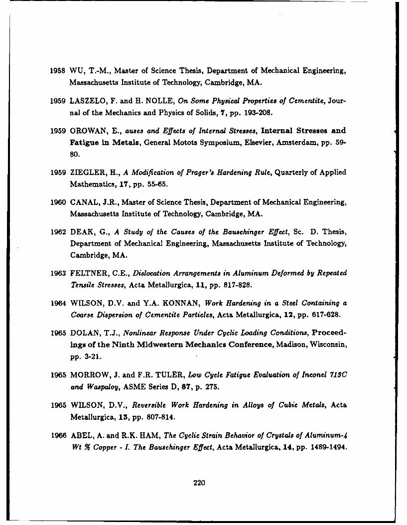
1958 WU, T.-M., Master of Science Thesis, Department of Mechanical Engineering,

Massachusetts Institute of Technology, Cambridge, MA.

1959 LASZELO, F. and H. NOLLE, On Some Physical Properties of Cementite, Jour-

nal of the Mechanics and Physics of Solids, 7, pp. 193-208.

1959 OROWAN, E., auses and Effects of Internal Stresses, Internal Stresses and

Fatigue in Metals, General Motots Symposium, Elsevier, Amsterdam, pp. 59-

80.

1959 ZIEGLER, H., A Modification of Prager's Hardening Rule, Quarterly of Applied

Mathematics, 17, pp. 55-65.

1960 CANAL, J.R., Master of Science Thesis, Department of Mechanical Engineering,

Massachusetts Institute of Technology, Cambridge, MA.

1962 DEAK, G., A Study of the Causes of the Bauschinger Effect, Sc. D. Thesis,

Department of Mechanical Engineering, Massachusetts Institute of Technology,

Cambridge, MA.

1963 FELTNER, C.E., Dislocation Arrangements in Aluminum Deformed by Repeated

Tensile Stresses, Acta Metallurgica, 11, pp. 817-828.

1964 WILSON, D.V. and Y.A. KONNAN, Work Hardening in a Steel Containing a

Coarse Dispersion of Cementite Particles, Acta Metallurgica, 12, pp. 617-628.

1965 DOLAN, T.J., Nonlinear Response Under Cyclic Loading Conditions, Proceed-ings of the Ninth Midwestern Mechanics Conference, Madison, Wisconsin,

pp. 3-21.

1965 MORROW, J. and F.R. TULER, Low Cycle Fatigue Evaluation of Inconel 713Cand Waspaloy, ASME Series D, 87, p. 275.

1965 WILSON, D.V., Reversible Work Hardening in Alloys of Cubic Metals, Acta

Metallurgica, 13, pp. 807-814.

1966 ABEL, A. and R.K. HAM, The Cyclic Strain Behavior of Crystals of Aluminum-4

Wt % Copper - L The Bauschinger Effect, Acta Metallurgica, 14, pp. 1489-1494.

220

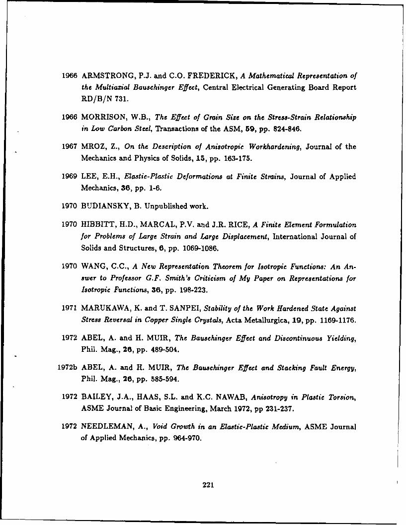
1966 ARMSTRONG, P.J. and C.O. FREDERICK, A Mathematical Representation ofthe Multiazial Bauschinger Effect, Central Electrical Generating Board Report

RD/B/N 731.

1966 MORRISON, W.B., The Effect of Grain Size on the Stress-Strain Relationshipin Low Carbon Steel, Transactions of the ASM, 59, pp. 824-846.

1967 MROZ, Z., On the Description of Anisotropic Workhardening, Journal of theMechanics and Physics of Solids, 15, pp. 163-175.

1969 LEE, E.H., Elastic-Plastic Deformations at Finite Strains, Journal of Applied

Mechanics, 36, pp. 1-6.

1970 BUDIANSKY, B. Unpublished work.

1970 HIBBITT, H.D., MARCAL, P.V. and J.R. RICE, A Finite Element Formulation

for Problems of Large Strain and Large Displacement, International Journal of

Solids and Structures, 6, pp. 1069-1086.

1970 WANG, C.C., A New Representation Theorem for Isotropic Functions: An An-

swer to Professor G.F. Smith's Criticism of My Paper on Representations for

Isotropic Functions, 36, pp. 198-223.

1971 MARUKAWA, K. and T. SANPEI, Stability of the Work Hardened State AgainstStress Reversal in Copper Single Crystals, Acta Metallurgica, 19, pp. 1169-1176.

1972 ABEL, A. and H. MUIR, The Bauschinger Effect and Discontinuous Yielding,

Phil. Mag., 26, pp. 489-504.

1972b ABEL, A. and H. MUIR, The Bauschinger Effect and Stacking Fault Energy,

Phil. Mag., 26, pp. 585-594.

1972 BAILEY, J.A., HAAS, S.L. and K.C. NAWAB, Anisotropy in Plastic Torsion,

ASME Journal of Basic Engineering, March 1972, pp 231-237.

1972 NEEDLEMAN, A., Void Growth in an Elastic-Plastic Medium, ASME Journal

of Applied Mechanics, pp. 964-970.

221

1973 HUTCHINSON, J.W., Finite Strain Analysis of Elastic-Plastic Solids and Struc-

tures, Numerical Solution of Nonlinear Structural Problems, R.F. Har-

tung ed., pp. 17-29.

1973 KISHI, T. and T. TANABE, The Bauschinger Effect and its Role in Mechanical

Anisotropy, Journal of the Mechanics and Physics of Solids, 21, pp. 303-315.

1973 TANAKA, K. MATSUOKA, S., SUZUKI, H. and T. NAKAMURA, The Work

Hardening Rate of Pearlitic Steel, Scripta Metallurgica, 7, pp. 799-802.

1974 ATKINSON, J.D. BROWN, L.M. and W.M. STOBBS, The Work-Hardening of

Copper-Silica IV. The Bauschinger Effect and Plastic Relaxation, Phil. Mag.

30, pp. 1247.

1974 FARDSHISHEH, F. and E.T. ONAT, Representation of Elastoplastic Behavior

by Means of State Variables, Problems of Plasticity, Sawczuk, A. ed., Leyden:

Noordhoff, pp. 89-115.

1974 GOULD, D., HIRSCH, P.B. and F.J. HUMPHREYS, The Bauschinger Effect,

Work-Hardening and Recovery in Dispersion Hardened Copper Crystals, Phil.

Mag., pp. 1353-1377.

1974 HASEGAWA, T. and T. YAKOU, Region of Constant Flow Stress During Com-pression of Aluminum Polycrystals Prestrained by Tension, Scripta, Metallurgica,

8, pp. 951-954.

1974 PHILLIPS, A., TANG, J.-L. and M. RICCIUTI, Acta Mechanica, 20, pp. 23-39.

1974 STOLTZ, R.E. and R.M. PELLOUX, Cyclic Deformation and Bauschinger Effect

in Al-Cu-Mg Alloys, Scripta Metallurgica, 8, pp. 269-276.

1975 HASEGAWA, T., YAKOU, T. and S. KARASHIMA, Deformation Behavior and

Dislocation Structures Upon Stress Reversal in Polycrystalline Aluminum, Mate-

rial Science and Engineering, 20, pp. 267-276.

1975 IBRAHIM, N. and J.D. EMBURY, The Bauschinger Effect in Single Phase B.C. C.

Materials, Materials Science and Engineering, 19, pp. 147-149.

1975 KRIEG, R.D., A Practical Two Surface Plasticity Theory, ASME Journal of

Applied Mechanics, 47, pp. 641-646.

222

1975 McMEEKING, R.M. and J.R. RICE, Finiet-Element Formulations for Problems

of Large Elastic-Plastic Deformation, International Journal of Solids and Struc-

tures, II, pp. 601-616.

1975 MORI, T. and K. NARITA, Decrease of Back Stress and Softening of Work

Hardened Copper-Silica Crystals by Recovery, Acta Metallurgica, 23, pp. 85-91.

1976 ANAND, L. and J. GURLAND, Strain-Hardening of Spheroidized High Carbon

Steels, 24, pp. 901-909.

1976 DAFALIAS, Y.F. and E.P. POPOV, Plastic Internal Variables Formalism of

Cyclic Plasticity, ASME Journal of Applied Mechanics, 43, pp. 645-651.

1976 DIETER, G.E., Mechanical Metallurgy, 2nd Edition, McGraw-Hill.

1976 HECKER, S.S., Experimental Studies of Yield Phenomena in Biaxially LoadedMetals, Constitutive Equations in Viscoplasticity, ASME AMD Vol. 20,

, ?. 1-33.

1976 LIU, K.C. and W.L. GREENSTREET, Experimental Studies to Examine Elastic-Plastic Behaviors of Metal Alloys Used in Nuclear Structures, Constitutive

Equations in Viscoplasticity, ASME AMD Vol. 20, pp. 35-56.

1976 MROZ, Z. SHRIVISTAVA, H.P. and R.N. DUBEY, A Non-Linear HardeningModel and Its Application to Cyclic Loading, Acta Mechanica, 25, pp. 51-61.

1977 KEY, S.W., BIFFLE, J.H. and R.D. KRIEG, A Study of the Computational andTheoretical Differences of Two Finite Strain Elastic-Plastic Models, Formula-

tions and Computational Algorithms In Finite Element Analysis, Bathe,Oden and Wunderlich, eds., Massachusetts Institute of Technology.

1977 LLOYD, D.J., The Bauschinger Effect in Polycrystalline Aluminum ContainingCoarse Particles, Acta Metallurgica, 25, pp. 459-466.

1977 PECKNER, D. and I.M. BERNSTEIN, Handbook of Stainless Steels, McGraw-

Hill.

1978 CHANG, Y.W. and R.J. ASARO, Bauschinger Effects and Work-Hardening in

Spheroidized Steels, Metal Science, pp. 277-284.

223

1978a LAMBA, H.S. and O.M. SIDEBOTTOM, Cyclic Plasticity for Nonproportional

Paths: Part 1 - Cyclic Hardening, Erasure of Memory, and Subsequent Strain

Hardening Experiments, ASME Journal of Engineering Materials and Technology,

100, pp. 96-103.

1978b LAMBA, H.S. and O.M. SIDEBOTTOM, Cyclic Plasticity for Nonproportional

Paths: Part 2 - Comparison With Predictions of Three Incremental PlasticityModels, ASME Journal of Engineering Materials and Technology, 100, pp. 104-111.

1978 TVERGAARD, V., Effect of Kinematic Hardening on Localized Necking in Bi-

axially Stretched Sheets, International Journal of Mechanical Science, 20, pp.

651-658.

1979 CHABOCHE, J.L., DANG VAN, K. and G. CORDIER, Modelization of the

Strain Memory Effect on the Cyclic Hardening of 916 S.S., SMIRT5, Div. L

Berlin.

1979 CHRISTOFFERSEN, J. and J.W. HUTCHINSON, A Class of Phenomenological

Corner Theories of Plasticity, Journal of the Mechanics and Physics of Solids, 27,p. 465.

1979 DIENES, J.K., On the Analysis of Rotation and Stress Rate in Deforming Bodies,

Acta Mechanica, 32, pp. 217-232.

1979 KANAZAWA, K., MILLER, K.J. and M.W. BROWN, Cyclic Deformation of 1%Cr-Mo- V Steel Under Out-of-Phase Loads, Fatigue of Engineering Materials andStructures, 2, pp. 217-228.

1979 KEY, S.W., KRIEG, R.D. and K.-J. BATHE, On the Application of the Finite

Element Method to Metal Forming Processes - Part I, Computer Methods in

Applied Mechanics and Engineering, 17/18, pp. 597-608.

1979 PHILLIPS, A. and C.W. LEE, Yield Surfaces and Loading Surfaces, Experiments

and Recommendations, International Journal of Solids and Structures, 15, pp.

715-729.

1979 SOWERBY, R., UKO, D.K. and Y. TOMITA, A Review of Certain Aspects of the

Bauschinger Effect in Metals, Materials Science and Engineering, 41, pp. 43-58.

224

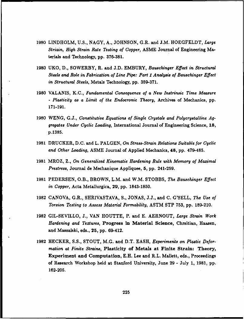
1980 LINDHOLM, U.S., NAGY, A., JOHNSON, G.R. and J.M. HOEGFELDT, Large

Striain, High Strain Rate Testing of Copper, ASME Journal of Engineering Ma-

terials and Technology, pp. 376-381.

1980 UKO, D., SOWERBY, R. and J.D. EMBURY, Bausehinger Effect in Structural

Steels and Role in Fabrication of Line Pipe: Part I Analysis of Bauschinger Effectin Structural Steels, Metals Technology, pp. 359-371.

1980 VALANIS, K.C., Fundamental Consequence of a New Intrinsic Time Measure

- Plasticity as a Limit of the Endocronic Theory, Archives of Mechanics, pp.

171-191.

1980 WENG, G.J., Constitutive Equations of Single Crystals and Polycrystalline Ag-gregate. Under Cyclic Loading, International Journal of Engineering Science, 18,

p.1385.

1981 DRUCKER, D.C. and L. PALGEN, On Stress-Strain Relations Suitable for Cyclicand Other Loading, ASME Journal of Applied Mechanics, 48, pp. 479-485.

1981 MROZ, Z., On Generalized Kinematic Hardening Rule with Memory of Maximal

Prestress, Journal de Mechanique Appliquee, 5, pp. 241-259.

1981 PEDERSEN, O.B., BROWN, L.M. and W.M. STOBBS, The Bauschinger Effect

in Copper, Acta Metallurgica, 29, pp. 1843-1850.

1982 CANOVA, G.R., SHRIVASTAVA, S., JONAS, J.J., and C. G'SELL, The Use of

Torsion Testing to Assess Material Formability, ASTM STP 753, pp. 189-210.

1982 GIL-SEVILLO, J., VAN HOUTTE, P. and E. AERNOUT, Large Strain Work

Hardening and Textures, Progress in Material Science, Chrsitian, Haasen,

and Massalski, eds., 25, pp. 69-412.

1982 HECKER, S.S., STOUT, M.G. and D.T. EASH, Experiments on Plastic Defor-

mation at Finite Strains, Plasticity of Metals at Finite Strain: Theory,Experiment and Computation, E.H. Lee and R.L. Mallett, eds., Proceedings

of Research Workshop held at Stanford University, June 29 - July 1, 1981, pp.

162-205.

225

1982 KANEKO, K., OGAWA, K. and K. IWATA, Evaluation of Inelastic Constitutive

Models for Breeder Reactor Design Practices - Part I: Plasticity Models, ASMEPVP Special Publication, Orlando, Florida.

1982 NAGTEGAAL, J.C. and J.E. DEJONG, Some Aspects of Non-Isotropic Workhard-

ening in Finite Strain Plasticity, Proceedings of the Workshop on Plasticity ofMetals at Finite Strain: Theory, Experiment and Computation, E.H. Lee and

R.L. Mallett, eds., Stanford University, pp. 55.

1982 SHRIVASTAVA, S.C., JONAS, J.J. and G. CANOVA, Equivalent Strain in LargeDeformation Torsion Testing: Theoretical and Practical Considerations, Journalof the Mechanics and Physics of Solids, 30, pp. 75-90.

1982 TVERGAARD, V., On Localization in Ductile Materials Containing SphericalVoids, International Journal of Fracture, 18, pp. 237.

1983 ASARO, R.J., Micromechanics of Crystals and Polycrystals, Advances in Ap-

plied Mechanics, 23, p. 1.

1983 CHABOCHE, J.L. and G. ROUSSELIER, On the Plastic and Viscoplastic Con-stitutive Equations. Part I: Rules Developed with Internal Variable Concept. Part

II: Application of Internal Variable Concepts to the 316 Stainless Steel, ASMEJournal of Pressure Vessel Technology, 105, pp. 153-164.

1983 CHAIT, R. and R. PAPIRNO, Compression Testing of Homogeneous Ma-terials and Composites, ASTM STP 808.

1983 HOSFORD, W.F. and R.M. CADDELL, Metal Forming, Mechanics andMetallurgy, Prentice-Hall.

1983 LEE, E.H., MALLETT, R.L. and T.B. WERTHEIMER, Stress Analysis forAnisotropic Hardening in Finite-Deformation Plasticity, ASME Journal of Ap-plied Mechanics, 50, pp. 554-560.

1983 LORET, B., On the Effect of Plastic Rotation in the Finite Deformation ofAnisotropic Elastoplastic Materials, Mechanics of Materials, 2, pp. 287-304.

1983 LOWE, T.C. and A.K. MILLER, The Nature of Directional Strain Softening,

Scripta Metallurgica, 17, pp. 1177-1182.

226

1983 MROZ, Z., Hardening and Degradation Rules for Metals Under Monotonic and

Cyclic Loading, ASME Journal of Engineering Materials and Technology, 105,

pp. 113-118.

1983 TSENG, N.T. and G.C. LEE, Simple Plasticity Model of Two-Surface Type,ASCE Journal of Engineering Mechanics, 109 , pp. 795-810.

1984 ABAQUS Theory Manual, version 4.6, Hibbitt, Karlsson and Sorensen, Inc.,

Frovidence, RI.

1984 BELL, J.F., Mechanics of Solids: Volume 1, The Experimental Founda-tions of Solid Mechanics, Germany, Springer-Verlag.

1984 CAILLETAUD, G., KACZMAREK, H. and H. POLICELLA, Some Elements on

Multiaxial Behavior of 316L Stainless Steel at Room Temperature, Mechanics of

Materials, 3, pp. 333-347.

1984a DAFALIAS, Y.F., A Missing Link in the Formulation and Numerical Imple-mentation of Finite- Transformation Elastoplasticity, Constitutive Equations:

Macro and Computational Aspects, William, K.J., ed., ASME, pp.25-40.

1984b DAFALIAS, Y.F., Modelling Cyclic Plasticity: Simplicity Versus Sophistication,

Mechanics of Engineering Materials, C.S. Desai and R.H. Gallagher, eds.,

Wiley.

1984c DAFALIAS, Y.F., The Plastic Spin Concept and a Simple Illustration of Its Rolein Finite Plastic Transformations, Mechanics of Materials, 3, pp. 223-233.

1984 JOHNSON, G.C. and D.J. BAMMAN, A Discussion of Stress Rates in Finite

Deformation Problems, International Journal of Solids and Structures, 20, pp.

725-737.

1984 KREMPL, E. and H. LU, The Hardening and Rate-Dependent Behavior of Fully

Annealed AISI Type 904 Stainless Steel Under Biazial In-Phase and Out-of-Phase

Strain Cycling at Room Temperature, ASME Journal of Engineering Materials

and Technology, 106, pp. 376-382.

1984 LOWE, T.C. and A.K. MILLER, Improved Constitutive Equations for ModelingStrain Softening - Part I: Conceptual Development, ASME Journal of Engineering

Materials and Technology, 106, pp. 337-342.

227

1984 MONTHEILLET, F., COHEN, M. and J.J. JONAS, Axial Stresses and Texture

Development During the Torsion Testing of Al, Cu and a-Fe, Acta Metallurgica,

32, pp. 2077-2089.

1984 PHILLIPS, A. and W.-Y. LU, An Experimental Invegation of Yield Surfaces of

Pure Aluminum with Stress-Controlled and Strain-Controlled Paths of Loading,

ASME Journal of Engineering Materials and Technology, 106, p. 349.

1985 ANAND, L., Constitutive Equations for Hot-Working of Metals, International

Journal of Plasticity, 1, pp. 213-232.

1985 CANOVA, G.R., KOCKS, U.F., TOME, C.N. and J.J. JONAS, Journal of the

Mechanics and Physics of Solids, 33, p. 371.

1985a DAFALIAS, Y.F., The Plastic Spin, ASME Journal of Applied Mechanics, 52,

pp. 865-871.

1985b DAFALIAS, Y.F., A Missing Link in the Macroscopic Constitutive Formulation

of Large Plastic Deformations, Plasticity Today, Sawxzuk, A., Bianchi, G.,

eds., Elsevier.

1985 MCDOWELL, D.L., An Experimental Study of the Structure of Constitutive

Equations for Nonproportional Cyclic Plasticity, ASME Journal of Engineering

Materials and Technology, 107, pp. 307-315.

1985 NOUHAILHAS, D., CHABOCHE, J.L., SAVALLE, S. and G. CAILLETAUD, On

the Constitutive Equations for Cyclic Plasticity Under Nonproportional Loading,

International Journal of Plasticity, 1, pp. 317-330.

1985 OGAWA, K., Mechanical Behavior of Metals Urder Tension-Compression Load-

ing at High Strain Rate, International Journal of Plasticity, 1, pp. 347-358.

1985 PAULUN, J.E. and R.B. PECHERSKI, Study of Corotational Rates for Kine-

matic Hardening in Finite Deformation Plaetictiy, Archives of Mechanics, 37,

pp. 661-677.

1985 REED, K.W. and S.N. ATLURI, Constitutive Modeling and Computational Im-

plementation in Finite Strain Plasticity, International Journal of Plasticity, 1,

pp. 63-87.

228

1985 STOUT, M.G., MARTIN, P.L., HELLING, D.E. and G.R. CANOVA, Multiaxial

Yield Behavior of 1100 Aluminum Following Various Magnitudes of Prestrain,

International Journal of Plasticity, 1, pp. 163-174.

1985 SWEARENGEN, J.C. and J.H. HOLBROOK, Internal Variable Model3 for Rate-

Independent Plasticity: Analysis of Theory and Experiment, Res Mechanica, 13,

pp. 93-128.

1986 BATE, P.S. and D.V. WILSON, Analysis of the Bauschinger Effect, Acta Metal-

lurgica, 34, pp. 1097-1105.

1986 CHABOCHE, J.L., Time-Independent Constitutive Theories for Cyclic Plasticity,

International Journal of Plasticity, 2, pp. 149-188.

1986 DIENES, J.K., A Discussion of Material Rotation and Stress Rate, Acta Mechan-

ica, 65, pp. 1-11.

1986 HAGHI, M., Deformation Behaviour of Iron Based ODS Superalloy MA956, Mas-

ter of Science Thesis, Massachusetts Institute of Technology, Cambridge, MA,

June, 1986.

1986 HAUPT, P. and C. TSAKMAKIS, On Kinematic Hardening and Large Plastic

Deformations, International Journal of Plasticity, 2, pp. 279-293.

1986 HELLING, D.E., MILLER, A.K. and M.G. STOUT, An Experimental Investi-gation of the Yield Loci of 1100-0 Aluminum, 70:50 Brass, and an Overaged

2024 Aluminum Alloy After Various Prestrains, ASME Journal of Engineering

Materials and Technology, 108, pp. 313-320.

1986 LU, W.-Y., Plastic Flow Under Multiaxial Cyclic Loading, Experimental Mechan-

ics, 26, pp. 224-229.

1986 WANTANABE, 0. and S.N. ATLURI, Internal Time, General Internal Vari-

able, and Multi- Yield-Surface Theories of Plasticity and Creep: A Unification of

Concepts, International Journal of Plasticity, 2, pp. 37-57.

1986 WILSON, D.V. and P.S. BATE, Reversibility in the Work Hardening of Spheroidised

Steels, Acta Metallurgica, 34, pp. 1107-1120.

229

1987 AGAH-TEHRANI, A., LEE, E.H., MALLETT, R.L. and E.T. ONAT, The The-

ory of Elastic-Plastic Deformation at Finite Strain with Induced Anisotropy Mod-

eled as Combined Isotropic-Kinematic Hardening, Journal of the Mechanics and

Physics of Solids, 35, pp. 519-539.

1987 BENALLAL, A. and D. MARQUIS, Constitutive Equations for Nonproportional

Cyclic, Elasto- Viscoplasticity, ASME Journal of Engineering Materials and Tech-

nology, 109, pp. 326-336.

1987 BROWN, S.B., An Internal Variable Constitutive Model for the Hot Working of

Metals, Ph.D. Thesis, Massachusetts Institute of Technology, April, 1987.

1987 CHU, C.-C., The Analysis of Multiaxial Cyclic Problems with an Anisotropic

Hardening Model, International Journal of Solids and Structures, 23, pp. 569-

579.

1987 DAFALIAS, Y.F., Issues on the Constitutive Formulation at Large Elastoplastic

Deformations, Part I: Kinematics, Acta Mechanica, 69, pp. 119-138.

1987 KOBAYASHI, H. and B. DODD, Estimation of Errors in Torsion Testing, Res

Mechanica, 20, pp. 163-175.

1987 LIPKIN, J., CHIESA, M.L. and D.J. BAMMANN, Thermal Softening of 304L

Stainless Steel: Experimental Results and Numerical Simulations, Proceedings of

IMPACT '87, Bremen, FRG, May, 1987.

1987 MCDOWELL, D.L., An Evaluation of Recent Developments in Hardening and

Flow Rules for Rate-Independent, Nonproportional Cyclic Plasticity, ASME Jour-

nal of Applied Mechanics, 54, pp. 323-334.

1987 NEEDLEMAN, A., A Continuum Model for Void Nucleation by Inclusion Debond-

ing, ASME Journal of Applied Mechanics, 54, p. 525.

1987 PAULUN, J.E. and R.B. PECHERSKI, On the Application of the Plastic Spin

Concept for the Description of Anisotropic Hardening in Finite Deformation Plas-

ticity, International Journal of Plasticity, 3, pp. 303-314.

1988 ASTM Standard E209-65, American Society of Testing and Materials.

230

1988 BOYCE, M.C., WEBER, G.G. and D.M. PARKS, On the Kinematics of Finite

Strain Plasticity, Submitted to the Journal of the Mechanics and Physics of Solids.

1988 BRONKHORST, C., A Study of the Bauschinger Effect and Cyclic Plasticity in

Spheroidized Steels, Master of Science Thesis, Massachusetts Institute of Tech-

nology, Cambridge, MA, March, 1988.

1988 MEGAHED, M.M., A Critical Examination of Nesting, Bounding and Memory

Surface/s Plasticity Theories Under Nonproportional Loading Conditions, Inter-

national Journal of Mechanical Engineering Science, 30, pp. 101-118.

1988 TRAMPCZYNSKI, W., The Experimental Verification of the Evolution of Kine-

matic and Isotropic Hardening in Cyclic Plasticity, Journal of the Mechanics and

Physics of Solids, 36, pp. 417-441.

231

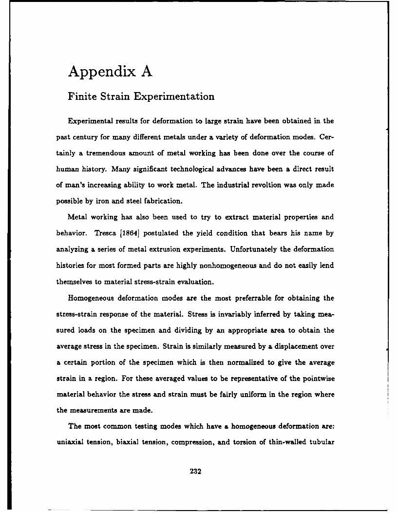
Appendix A

Finite Strain Experimentation

Experimental results for deformation to large strain have been obtained in the

past century for many different metals under a variety of deformation modes. Cer-

tainly a tremendous amount of metal working has been done over the course of

human history. Many significant technological advances have been a direct result

of man's increasing ability to work metal. The industrial revoltion was only made

possible by iron and steel fabrication.

Metal working has also been used to try to extract material properties and

behavior. Tresca [18641 postulated the yield condition that bears his name by

analyzing a series of metal extrusion experiments. Unfortunately the deformation

histories for most formed parts are highly nonhomogeneous and do not easily lend

themselves to material stress-strain evaluation.

Homogeneous deformation modes are the most preferrable for obtaining the

stress-strain response of the material. Stress is invariably inferred by taking mea-

sured loads on the specimen and dividing by an appropriate area to obtain the

average stress in the specimen. Strain is similarly measured by a displacement over

a certain portion of the specimen which is then normalized to give the average

strain in a region. For these averaged values to be representative of the pointwise

material behavior the stress and strain must be fairly uniform in the region where

the measurements are made.

The most common testing modes which have a homogeneous deformation are:

uniaxial tension, biaxial tension, compression, and torsion of thin-walled tubular

232

specimens. In each of these tests the stresses and strains are 'uniform' throughout

the gauge region.

The biggest problem to obtaining useful experimental results for large strain

deformation is the significant geometry changes that generally accompany flow. A

discussion of many of the limitations of different testing modes is given in a recent

review by Hecker, Stout and Eash [1982].

A number of inhomogeneous and indirect tests have also been used to infer

large strain results. Two such tests having inhomogeneous deformation are the

solid rod torsion test and the post necking tensile test. Analysis techniques are

available (Bridgman [1943], Nadai [1931]) to obtain the stress-strain results but

certain assumptions are made about the material behavior which are too restrictive.

Indirect tests have been used to obtain results to the very largest strains. An

indirect test is one in which the specimen is deformed in some mode such as wire

drawing or plate rolling to a large prestrain. It is then unloaded and the effect

of the prestrain is determined by testing in a mode where the yield can easily be

determined such as uniaxial tension. The locus of these yield stresses for various

prestrains is plotted as a stress-strain result. This type of analysis makes many

assumptions about the material behavior and is not appropriate for studying the

details of that behavior.

Of the direct, homogeneous testing techniques the two which have seen the most

effective use are the uniaxial compression and thin-walled torsion tests. The tensile

test is by far the most widely used mechanical test to determine yield strengths but

it suffers from the geometric instability of necking. Few metals can be strained in

tension to even 40 or 50% strain before the localization occurs. Most metals can

233

not even sustain that much tensile strain. The strain hardening rate of the material

controls this instability point.

Uniaxial compression is used extensively to obtain flow stress values at large

strain (Brown [1987], Chait and Papirno [19831). Solid, cylindrical specimens are

compressed between smooth, flat platens in a controlled manner to obtain strains

approaching 100%. This strain range can even be increased by remachining the

specimens. Initially a specimen should have a length to diameter ratio of 1.5 to

1.6 . If it is larger than this plastic buckling may occur. During compression it is

important to maintain adequate lubrication between the specimen and platen. This

is necessary to achieve uniform straining and to prevent barrelling. The specimen

undergoes large geometry changes during compression. To achieve a true (logarith-

mic) strain of -100% the specimen must by compressed to 37% of its original height.

Nonetheless a significant amount of compression data is available in the literature

(Hecker, Stout and Eash [1982]; Gil Sevillano, van Houtte and Aernoudt 11982]).

The other testing mode used to generate a significant amount of large strain data

is torsion. The torsion test involves twisting a cylindrical specimen and recording

the torque required as a function of twist angle. For solid specimens, as noted

above, the reduction of the torque/twist to stress-strain results is very restrictive.

For example it is known that when twisting a specimen to large shear strain there is

a coupling between the response in the shear and axial direction. A specimen that

is unrestrained in the axial direction will elongate (Swift [1947]) and a specimen

prevented from elongating axially will develop either tensile or compressive stresses

[Montheillet, Cohen and Jonas, 19841. The magnitude of these axial effects are

important material characterizing parameters as will be demonstrated later in this

234

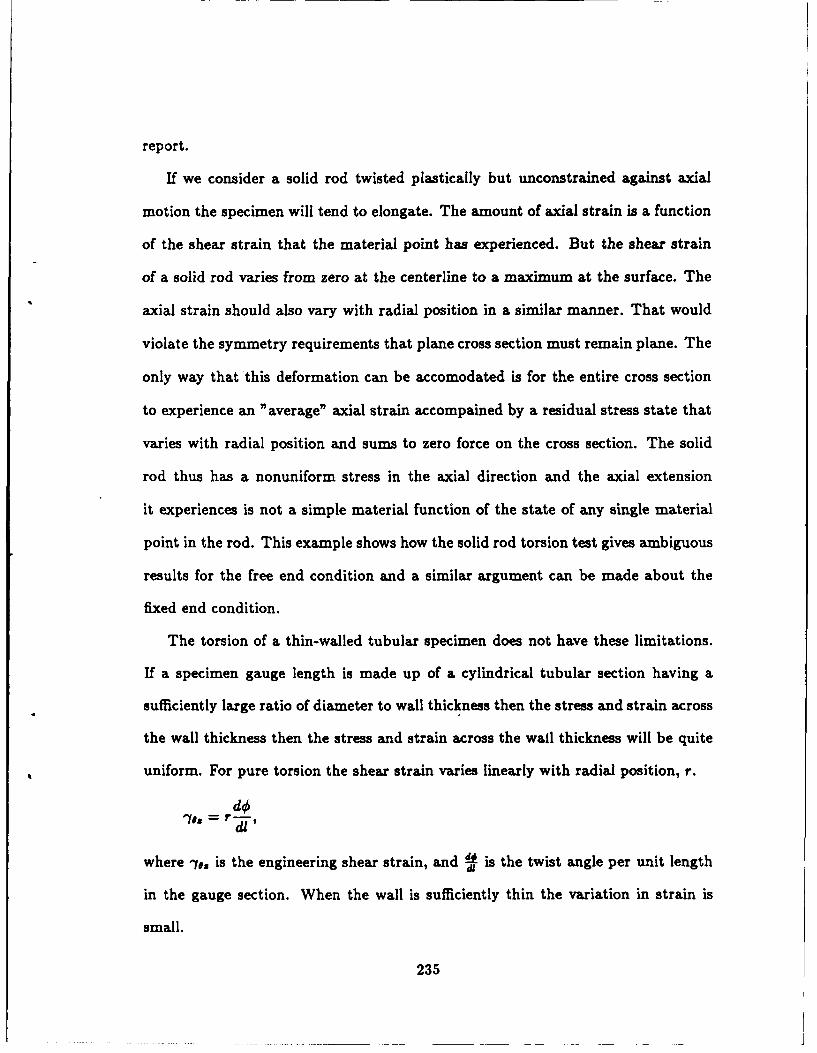
report.

If we consider a solid rod twisted plastically but unconstrained against axial

motion the specimen will tend to elongate. The amount of axial strain is a function

of the shear strain that the material point has experienced. But the shear strain

of a solid rod varies from zero at the centerline to a maximum at the surface. The

axial strain should also vary with radial position in a similar manner. That would

violate the symmetry requirements that plane cross section must remain plane. The

only way that this deformation can be accomodated is for the entire cross section

to experience an "average" axial strain accompained by a residual stress state that

varies with radial position and sums to zero force on the cross section. The solid

rod thus has a nonuniform stress in the axial direction and the axial extension

it experiences is not a simple material function of the state of any single material

point in the rod. This example shows how the solid rod torsion test gives ambiguous

results for the free end condition and a similar argument can be made about the

fixed end condition.

The torsion of a thin-walled tubular specimen does not have these limitations.

If a specimen gauge length is made up of a cylindrical tubular section having a

sufficiently large ratio of diameter to wall thickness then the stress and strain across

the wall thickness then the stress and strain across the wall thickness will be quite

uniform. For pure torsion the shear strain varies linearly with radial position, r.

7z= 7-,d/'

where -y#, is the engineering shear strain, and -d is the twist angle per unit lengthdi

in the gauge section. When the wall is sufficiently thin the variation in strain is

small.

235

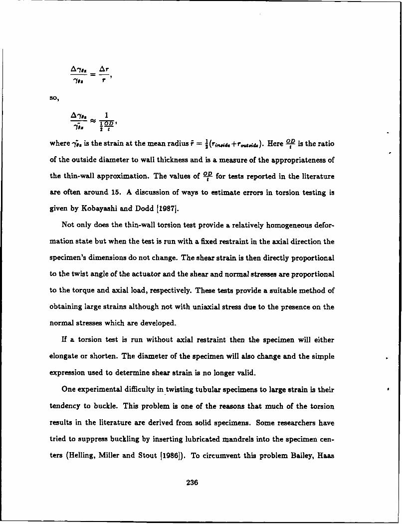
A-to. ArA/, _ r

SO,

o.z i -,*where j', is the strain at the mean radius F = (ri & + r ). Here 22 is the ratio

t

of the outside diameter to wall thickness and is a measure of the appropriateness of

the thin-wall approximation. The values of - for tests reported in the literature

are often around 15. A discussion of ways to estimate errors in torsion testing is

given by Kobayashi and Dodd (1987].

Not only does the thin-wall torsion test provide a relatively homogeneous defor-

mation state but when the test is run with a fixed restraint in the axial direction the

specimen's dimensions do not change. The shear strain is then directly proportional

to the twist angle of the actuator and the shear and normal stresses are proportional

to the torque and axial load, respectively. These tests provide a suitable method of

obtaining large strains although not with uniaxial stress due to the presence on the

normal stresses which are developed.

If a torsion test is run without axial restraint then the specimen will either

elongate or shorten. The diameter of the specimen will also change and the simple

expression used to determine shear strain is no longer valid.

One experimental difficulty in twisting tubular specimens to large strain is their

tendency to buckle. This problem is one of the reasons that much of the torsion

results in the literature are derived from solid specimens. Some researchers have

tried to suppress buckling by inserting lubricated mandrels into the specimen cen-

ters (Helling, Miller and Stout [1986]). To circumvent this problem Bailey, Haas

236

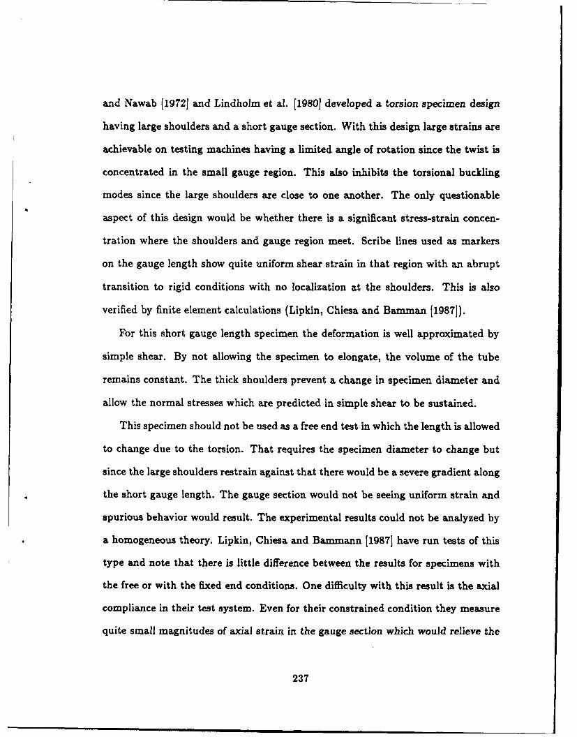
and Nawab (19721 and Lindholm et al. (19801 developed a torsion specimen design

having large shoulders and a short gauge section. With this design large strains are

achievable on testing machines having a limited angle of rotation since the twist is

concentrated in the small gauge region. This also inhibits the torsional buckling

modes since the large shoulders are close to one another. The only questionable

aspect of this design would be whether there is a significant stress-strain concen-

tration where the shoulders and gauge region meet. Scribe lines used as markers

on the gauge length show quite uniform shear strain in that region with an abrupt

transition to rigid conditions with no localization at the shoulders. This is also

verified by finite element calculations (Lipkin, Chiesa and Bamman [1987]).

For this short gauge length specimen the deformation is well approximated by

simple shear. By not allowing the specimen to elongate, the volume of the tube

remains constant. The thick shoulders prevent a change in specimen diameter and

allow the normal stresses which are predicted in simple shear to be sustained.

This specimen should not be used as a free end test in which the length is allowed

to change due to the torsion. That requires the specimen diameter to change but

since the large shoulders restrain against that there would be a severe gradient along

the short gauge length. The gauge section would not be seeing uniform strain and

spurious behavior would result. The experimental results could not be analyzed by

a homogeneous theory. Lipkin, Chiesa and Bammann [1987] have run tests of this

type and note that there is little difference between the results for specimens with

the free or with the fixed end conditions. One difficulty with this result is the axial

compliance in their test system. Even for their constrained condition they measure

quite small magnitudes of axial strain in the gauge section which would relieve the

237

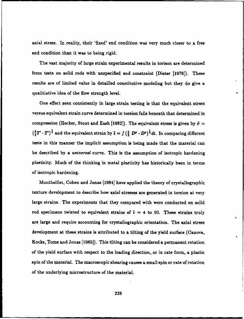
axial stress. In reality, their 'fixed' end condition was very much closer to a free

end condition than it was to being rigid.

The vast majority of large strain experimental results in torison are determined

from tests on solid rods with unspecified end constraint (Dieter [1976]). These

results are of limited value in detailled constitutive modeling but they do give a

qualitiative idea of the flow strength level.

One effect seen consistently in large strain testing is that the equivalent stress

versus equivalent strain curve determined in torsion falls beneath that determined in

compression (Hecker, Stout and Eash [1982]). The equivalent stress is given by j =

(IT'V. T') and the equivalent strain by i - f (I DP " DP) 1 dt. In comparing different

tests in this manner the implicit assumption is being made that the material can

be described by a universal curve. This is the assumption of isotropic hardening

plasticity. Much of the thinking in metal plasticity has historically been in terms

of isotropic hardening.

Montheillet, Cohen and Jonas [1984] have applied the theory of crystallographic

texture development to describe how axial stresses are generated in torsion at very

large strains. The experiments that they compared with were conducted on solid

rod specimens twisted to equivalent strains of i = 4 to 10. These strains truly

are large and require accounting for crystallographic orientation. The axial stress

development at these strains is attributed to a tilting of the yield surface (Canova,

Kocks, Tome and Jonas [1985]). This tilting can be considered a permanent rotation

of the yield surface with respect to the loading direction, or in rate form, a plastic

spin of the material. The macroscopic shearing causes a small spin or rate of rotation

of the underlying microstructure of the material.

238

The effect of a lower flow stress in torsion is seen at strains much less than these

where crystallographic texture is important. This has been a major motivation for

the work presented in this thesis. The traditional ideas of isotropic hardening can

not account for this yet much of the large plastic deformation in manufacturing or

ballistic penetration is done under a shearing action where this discrepancy is seen.

A better model of these experimentally observed results is sought in this work.

239

Appendix B

Review of Cyclic Plasticity Modeling

Prager-Ziegler kinematic hardening has the simplest explicit evolution

equation for the back stress.

B=CDP.

Here B is the back stress, D P the plastic stretching and C is generally a constant

(linear hardening). This is the most common theory employing a back stress and

has been incorporated into most nonlinear finite element codes.

The significant shortcomings of this model include its failure to give a smooth

elastoplastic transition during reverse loading, and its failure to develop a stable,

symmetric hysteresis loop under cycling. This model has been applied to large

strain deformation, often when combined with some form of isotropic hardening.

For such a model, the permanent softening is a measure of the back stress prior to

unloading. As discussed in section 2.2 recent work by Wilson &nd Bate [1986] show

that this is not what is occurring physically. The permanent softening is not a good

measure of the back stress in the lattice of the material.

Attempts have been made to generalize this model by letting C be a function

of plastic strain, C - &( ) . This leads to inconsistencies since there then exists

a unique relationship between the back stress and plastic strain [Chaboche,1986].

Other possibilities for functional dependence of C have not been generally explored.

This could be a fruitful area of research. What is required is for C to be such that

it gives the proper back stress increase during monotonic loading (which is a fairly

slow increase) and a rapid change in back stress during reversing. Currently this

240

does not exist so the Prager kinematic hardening rule is generally not used for

modeling cyclic behavior.

In the mechanical sublayer model a number of independent structural ele-

ments are deformed in parallel. Each element undergoes the same deformation but

by having different flow strength and hardening (isotropic) properties a composite

response is obtained. Models of this type have been proposed by Bessling [1953]

and Bate and Wilson [1986]. This modeling concept does not allow the development

of permanent softening although it does introduce a more gradual transition from

elastic to reverse plastic flow. In order to achieve a good match with experiments

many elements are required which adds many variables to the theory and increases

the complexity.

The Mroz model [Mroz,1967] consists of a series of nested surfaces which can

translate inside of one another. The plastic modulus is given as a function of the

size of the active surface. The active surface is the largest surface which the stress

point contacts. Once the active surface touches the next larger surface it no longer

is active but just translates along with the stress point. The direction that the

active surface translates in is given by the vector connecting the stress point with

the point on the next larger surface having the same outward normal n as the active

surface. This is illustrated in Figure B.I. This leads to a piecewise stress-strain

curve with a large number of surfaces required to obtain a good fit to experiment.

For uniaxial cycling this model captures many of the important features de-

scribed above (1-6) although it does poorly on the asymmetric cycling (7,8).

An important difference between the Mroz and Prager models is the direction

of yield surface translation. For multiaxial loading they can be quite different. This

241

will be brought out in more detail when considering multiaxial, nonproportional

cycling.

The two surface model was first introduced by Krieg [1975] and Dafalias and

Popov [1976]. Conceptually it is similar to the Mroz model since it contains one

surface (the yield surface) nested inside of the other (the bounding surface). In the

Mroz model the plastic modulus equals its constant value associated with the outer

active surface. In the two surface model the plastic modulus is given as a function

of the distance between the yield and bounding surfaces. As illustrated in Figure

B.2, when the loading direction is reversed the distance between the two surfaces is

measured between points on the corresponding surfaces having the same outward

normal n. The magnitude of this distance is given as 6 where 6,, represents this

value when plastic flow is reinitiated. The direction of motion of the yield surface is

given by the same rule as that of the Mroz model. That is, the direction of motion is

given by the vector connecting the corresponding points on the two surfaces having

the same n.

Dafalias and Popov [19761 have chosen to represent the plastic modulus, E., by

Ep = Ep+ ( n)( 6 )

Here E represents the plastic modulus before unloading from contact with the

bounding surface. Notice that this function satisfies the requirements for a smooth

elastoplastic transition.

b = bin EP --+ 0o,

6=0 Ep= E.

This model can be made to satisfy all of the criteria (1-7) although a small

partial reverse load followed by reloading can cause a significant stress overshoot.

242

This is discussed by Dafalias [1984b] and Chaboche [19861. The updating procedure

chosen by Dafalias and Popov [1976] leads to this overshoot but it is not a necessary

consequence of two surface models.

The evanscent hardening model is a phenomenological theory similar to

Prager-Ziegler hardening except that the back stress evolution law is modified.

B = C 1D P - C, 'B

Here the direction and magnitude of the motion of the yield surface are modified by

the back stress. This gives a direction similar to the Mroz or two surface models.

The functions C1 and C2 are taken to be constants or functions of plastic strain

EP. This theory has been used by Armstrong and Frederick [1966], Chaboche [1983]

and Nagtegaal and deJong [19821.

Here the back stress is removed more quickly during reverse flow than it builds

up during monotonic loading. The plastic modulus is larger when plastic flow

commences in the reverse direction than it had been during forward loading but

there is not a smooth elastoplastic transition. Also the theory predicts a saturation

of the back stress during uniaxial loading of Bf'* = C1/C 2 and no permanent

softening. This theory then does not satisfy requirements (2) or (4).

This model has been used to model the shape of cyclic curves at one strain range,

but often fails when the strain range is changed. The constant C2 determines both

how quickly the back stress builds up during monotonic loading and the degree

of rounding of the stress-strain curve during reversing. A large value of C2 is

needed to adequately model the large stiffness during reversing but a small C2 is

required for the correct build up of back stress. Chaboche and Rousselier [1983]

accomodated this by introducing several back stress variables, each with its own

243

evolution equation.

Bi = CjD P - c2 Bj.

This improves the uniaxial modeling but greatly increases the complexity and stor-e

age requirements.

The work of Chaboche and his coworkers has been extensive in applying evanes-

cent type models [Chaboche, 1986]. They have settled on a particular form where

C1 is a constant and C2 is an increasing function of plastic strain.

A variation of the evanescent hardening rule has been proposed by Mroz [1981,1983].

In order to account for the history effect of the previous maxiamum stress, a max-

imal back stress surface is introduced. This keeps track of the maximum value of

the equivalent back stress that has occured over the history of the deformation.

For de-formation occuring inside of this surface the isotropic component evolves to

an asymptotic value which could involve hardening or softening. The scalars C

and C2 are functions of the current, scalar equivalent back stress. Mroz claims

that the new parameter (maximal equivalent back stress) is a way of taking into

account the natural dependence of the Mroz model [Mroz, 1967] on the maximal

back stress. In the Mroz [1967] model this dependence is incorporated through the

relative configuration of the nested surfaces.

The endocronic, or internal time, theory of plasticity was first proposed and

used by Valanis in the 1970's [Valanis, 1980]. The theory uses an internal time

variable as the measure of the history of deformation. It is a measure of material

memory.

244

Many engineers have avoided the endocronic theory because it does not resemble

the more classical formulations. Plasticity laws have historically been formulated

in terms of incremental or flow relationships due to the nature of the deformation

process (dislocation glide in metals). The endocronic theory has been constructed

using integrals over the deformation history. It has received recent attention because

of its success in modeling some of the phenomena of cyclic plasticity.

Its success has derived from its flexibility of including many parameters to match

experiments. At the heart of the theory lies the equation for the deviatoric stress

T'.

T'= 2L p p(z - ' O p d',

where z is an internal time variable. The choice of the kernel p(z) provides the

flexibility of the model. Watanabe and Atluri [1986] showed that by proper choice

of p(z) the endocronic theory can be reduced, in its differential form, to any of the

following: Prager-Ziegler kinematic hardening, Mroz model, two surface model, or

evanescent hardening. The endocronic theory can then be seen as an overall frame-

work for use in expressing many theories. In application, a specific kernel function

must be postulated. This reduces the endocronic theory to more recognizablc form.

In general then, the endocronic theory can satisfy any of the requirements of

cyclic plasticity that the above models can. It does not make sense to discuss the

model without specifying a particular kernel p(z). Since the obvious kernels to use

reduce to one of the above models it is logical to just analyze the models in the

more recognizable flow formulation.

As discussed above, each of the models used for cyclic plasticity has certain

strengths and weaknesses. The choice of a model depends in part upon the phe-

245

nomena most important for a given application. The Mroz, two surface, and evanes-

cent models give qualitatively similar modeling capabalities. The two surface model

has the advantage of specifying a smooth elastoplastic transition and a better sim-

ulation of random-type loadings and ratchetting effects (Chaboche [19861). The

evanescent hardening model has the advantage of easier numerical implementation

and connection with internal variable theories. e

246

L 14

K

Figure B.1 Illustration of the Mroz [1967] model showing thepiecewise linear approximation to the stress-strain curve and its mul-tiaxial representation with nested yield surfaces.

247

(a)

A SOUND

TIELD S&PWAM

Figure B.2 Illustration of the two surface plasticity model. Boththe (a) one dimensional and (b) multiaxial representations are shown.

248

DISTRIBUTION LIST

No. ofCopies To

1 Office of the Under Secretary of Defense for Research and Engineering, The Pentagon,Washington, DC 20301

Commander, U.S. Army Materiel Command, 50nI Eisenhower Avenue, Alexandria, VA 22333-00011 ATTN: AMCLD

Commander, U.S. Army Laboratory Command, 2800 Powder Mill Road, Adeiphi, MD 20783-11451 ATTN: AMSLC-IM-TL

Commander, Defense Technical Information Center, Cameron Station, Building 5, 5010 DukeStreet, Alexandria, VA 22304-6145

2 ATTN: DTIC-FDAC

1 Metals and Ceramics Information Center, Battelle Columbus Laboratories, 505 King Avenue,Columbus, OH 43201

Commander, Army Research Office, P.O. Box 12211, Research Triangle Park, NC 27709-22111 ATTN: Information Processing Office

Commander, U.S. Army Electronics Technology and Devices Laboratory, Fort Monmouth,NJ 07703-5000

1 ATTN: SLCET-DT

Commander, U.S. Army Missile Command, Redstone Arsenal, AL 35898-52471 ATTN: AMSMI-RD-ST1 Technical Library

Commander, U.S. Army Armament, Munitions and Chemical Command, Dover, NJ 078012 ATTN: SMCAR-TDC

Commander, U.S. Army Natick Research, Development and Engineering Center, Natick,MA 01760

1 ATTN: Technical Library

Commander, U.S. Army Tank-Automotive Command, Warren, MI 48397-50001 ATTN: AMSTA-R

Commander, U.S. Army Engineer Waterways Experiment Station, P.O. Box 631, Vicksburg,MS 39180

1 ATTN: Research Center Library

Director, U.S. Army Ballistic Research Laboratory, Aberdeen Proving Ground, MD 210051 ATTN: SLCBR-DD-T (STINFO)1 SLCBR-IV-M, Dr. W. H.,DrysdaleI SLCBR-TB-W, Or. J. Walter1 SLCBR-TB-W, Dr. Thomas W. Wright

Director, Benet Weapons Laboratory, LCWSL, USA AMCCOM, Watervliet, NY 121891 ATTN: AMSMC-LCB-TL

Commander, U.S. Army Foreign Science and Technology Center, 220 7th Street, N.E.,Charlottesville, VA 22901-5396

I ATTN: AIAST-RA-ST

Director, Eustis Directorate, U.S. Army Air Mobility Research and Development Laboratory,Fort Eustis, VA 23604-5577

1 ATTN: SAVDL-E-MOS (AVSCOM)

Director, Langley Directorate, U.S. Army Air Mobility Research and Development Laboratory,NASA-Langley Research Center, Hampton, VA 23665

I ATTN: Aerostructures Directorate

Naval Research Laboratory, Washington, DC 203751 ATTN: Code 5830

Office of Naval Research, 800 North Quincy Street, Arlington, VA 22217-50001 ATTN: Mechanics Division, Code 1132-SM

No. ofCopies To

Naval Air Development Center, Warminster, PA 18974-50001 ATTN: Code 60641 AVCSTD/6043

U.S. Navy David Taylor Researcb Center, Bethesda, MO 200841 ATTN: Code 172

U.S. Air Force Office of Scientific Research, Boiling Air Force Base, Washington, DC 203321 ATTN: Mechanics Division

Commander, U.S. Air Force Materials Laboratory, Wright-Patterson Air Force Base, 0.9 454331 ATTN: AFWAL/MLLN

National Aeronautics and Space Administration, Marshall Space Flight Center, Huntsville,AL 35812

1 ATTN: EHO1, Oir, M&P lab

1 Committee on Marine Structures, Marine Board, National Research Council, 2101 ConstitutionAvenue, N.W., Washington, DC 20418

Director, U.S. Army Materials Technology Laboratory, Watertown, MA 02172-00012 ATTN: SLCMT-TML1 Author

i

C, -Cc a c c - W 00 u wzz0 0

7;!2 c a Ic MC-2m 1= a 40c '0

c CL 6 o u 0 41- I.C 0 W

t-z 03-- c 2.5-0 W a '0We- W vOM -16 c W 0 W

W, UO EWE 0.5-

0 CW u

od# I ,,u u 0364

quj a a 0 c 20-- c w- .2- vt! c 3% 2 -2 U4, c.6-0- . . . m c - 20 0 c W acra C-Oc..- W-- v c

cwcu wl- 2-.va 2 -.. 2 .0r 4 v 0 11 - z . - -,. - Cc or '0- -- I C. &C cL ".. .. , Sc .4.w 6 W0--w m 0

I TO OC u c; lot . u C. . a 1; 31 4'j p! - :;Ci I " u- u-0 .0

8 -z;x0 0>.,;; Im o 0 -:; w

Om -:; W - , W

CL 3_2006-O."Z-.0 Wc --- c t :.51;-- - CL M S'.O-Zcc t -- .-- I

2 .0 E0.1- O-C 0 W - W 0 W- .- C 0Zo .0 e z - - I cm co

0 V C =.Wz.WRo 0 M-M-mc

LD 0 W- 5.5 "'0 W C-CL- .10 0 I c c WW- 41 -W.CWC.zT .- C8:OH c z W -0 Cc z T W C Cc v 1.5-6>

U1.2 6 ; W= 0 W.2 U.50:5 -WO c,a- 41 14-- c x Z'-c 0 2 01

0-2 SOO 'pla-21"cW CLO 06 0 -0-0 W C.

ZM 60 C- -0 -C -Cow 0 W

W 04 147Z'; ' ' E 10 - m - 5 U60W>4T;t 6W-aolM. 9 c . . w. 0 .. 2 U 1 0 v -C v W W 0 1"Z 0 a-W, 214 1 W !0-- 6 v a, E -- m- -u, a . c

4-1 C -0 3=2 we - 20-4 R W -'s a c u 0 0 A 0 -0 If A 0 35 to IW-cm

=0 I= 14 it 10 WO-0 kl";-c - &% -c a cc . c 0 -4 c6L -a - -cn u =0 C- V t 0 IV00

cuW w m m WE '.5 c c w c CL bla 0

= 0-0 -C .0 E M 11 041 cn=C2 W . 87 . - Mo W W C

C3 -1012 IE M - W. Wowe Wa-X=o coz W 0 c c mm a,

c W0, WC-W 0,,5- IL cx r-= Wa -1 -6 -2 W0 W Z 0 V- r c WE W O.Cx u=I -C, W

C M. >, ME E Go": 0c a W c a mm o S =a 1.W- c =

:W5cc

o I W C 0

a c C- W 0 a a c W00 a 1 0 Q.0--a-- uc0-

r O-Z me 80 !!cc 6UruL-l -310- 04'% 11 .u > U0. 0 6 rL 0 1 2 -X

C c2ml=w- a- w 4, 7; C* 40M

0 0- C- CL 0 w a 03- C =;; 0 C

-z We0- .Z.2=,;; , " - 0--tz2-.2 . , C

4-1W a I C-0 M; = 0 cc Q- cm -. ; C.:; 0 14 W W 0 Ci.c xj 0 C v M E cOU 8.5 6 cc C,

CIOcz- 11 WeU. u . W- -Co- 'a W-W.%-

40:= c

a -0 W.C

-. 2 -, u .;, C CLW-0- . m u W aa a W-.5 W= c .2- c W=W c

C.S C 1 6 W 6- 39 C 0 U W c W c W c 0G.- a .0-. I- c - - -; 8 - I , - .2C W a c lu c "00WO 0 w 00IL c & - C.

3% u W M.C0 - . . 06 I.L - 4 . I '- - U me '0

.2 t CO W 1 31 N 3C U-2 U VV-ap=

- 0 -z; ua, 2 0 a C c 2 2 u 1 3-0 all Cw'&

M3-2,200 O-W-.Wc--CL c V.%CIO-,!cWOW- - c 0 c A .0cc c a v u 2 z co = I - 2 .0 W 0 W 0

6.MW 6 CL c

-V W:;

am A2 .- . 1 10-10",.0.0 c",='a UC21- o- lu c W o-ICIZ-40.1-5. - W

zc= 6 - Ic, lu C: 0-0 - w Zwf. - a ZZO " c:; 0 W- 6 u a

4,0 -41ZI- W ag .10-1; Ju W 0 0 m c W2 -. :; c

2:::2;:: lu 4 c .2 C>l I-C W 'M u -0- . ; C. C V C.

C2 -C .1 nm- c 1%zi 3 .C- 1.0 0 W.T.C.; L mlU.",i&OOWxxT;lW W 0 0

M.W %; t e clock W.Cuq-vft "; - w u W W W 0 00- .06- 4m a M O zZ4 we & W 0 0 =,a 4:5 C& v 0-- W 0) 6 41 W W u =10 M2 . a,

cc 0 2L W"bzllz 110 -'sV6 c I =5 a, 0 a TOO O ro-0 W u 0 u ICP& m 6 id .0 6 -:;

Vi 'a' "'0 Ck "'; 'c b c c 0 . m cW -V .0 M 10 W 1 1 2-5-2-2-X 31910 M-0 - U, 11 SWI CLS 10 0

0 0 'OC *; .1 - 0ImlWE= W 0 V. K'..8 W TO 41 m I v W--c 0-M w- m-

0 x 2Rg -0- f " , - r

oc-w = a c c - a m W 0- 60 W a, 'cc -C o C

0, W-T

m IW 7 v -0 -9 Cc - M. I "n Vo 0 wc W - c W- m ft 4) -Co-as -4 =4 . W - i c

r1-7 F.::, i '0 W5, 0 W 41 WC . - C - CWI - 4tosuffiW . - V W

u W voC- 0 W-vu I CIO a 0