Designing around storytelling - Design + banter, 09 April 2014
CSCI-GA.2270-001 - Computer Graphics - Fall 16 - Daniele Panozzo
09 - Designing Surfaces
CSCI-GA.2270-001 - Computer Graphics - Fall 16 - Daniele Panozzo
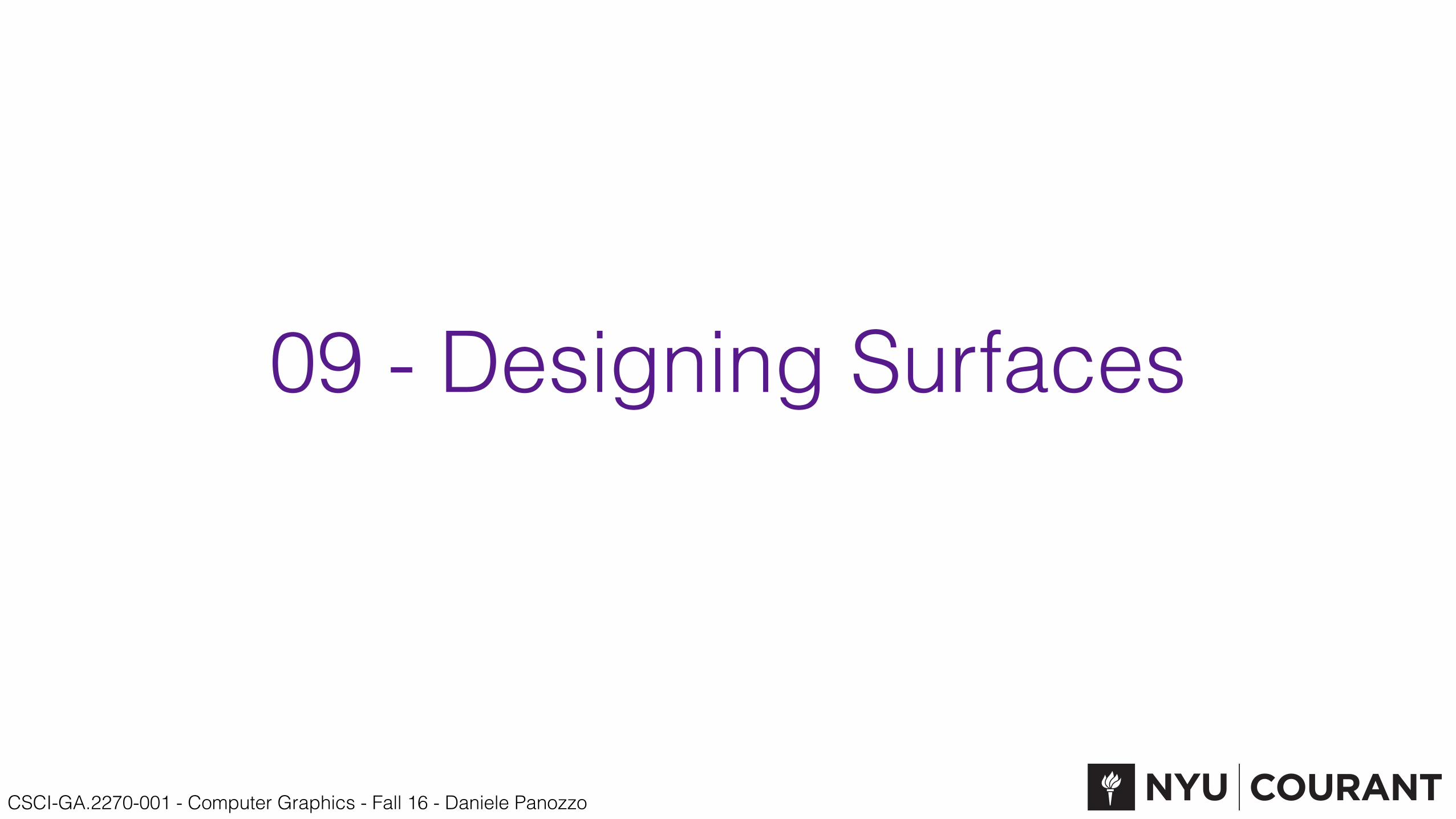
Triangular surfaces• A surface can be discretized by a collection of points and triangles
• Each triangle is a subset of a plane
• Every point on the surface can be expressed as an affine combination of three vertices
• The surface is C0
CSCI-GA.2270-001 - Computer Graphics - Fall 16 - Daniele Panozzo
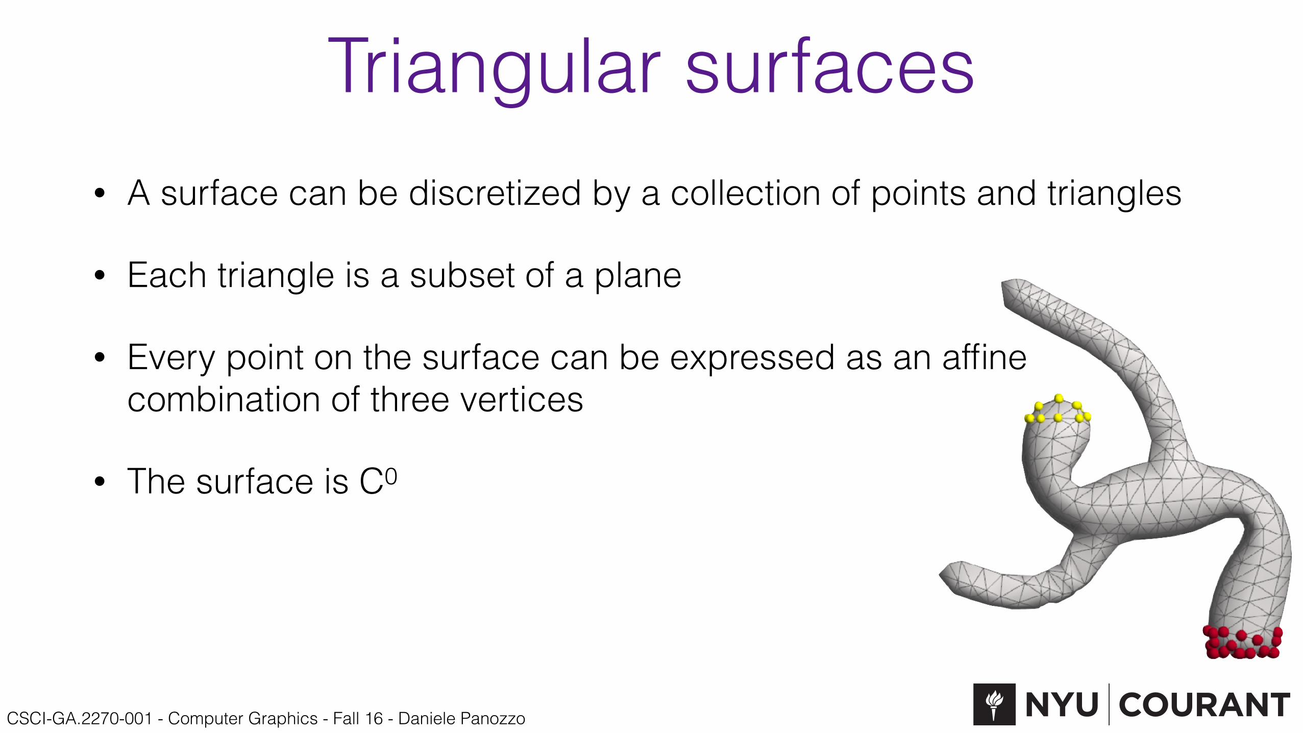
Barycentric coordinates• The points inside a triangle, are usually parametrized using barycentric
coordinates w:
• The barycentric coordinates naturally defines a parametrization
v1
v2
v3
p
w1
w2
w3
px
py=
11 1 1
v1y v2y v3y
v1x v2x v3x
CSCI-GA.2270-001 - Computer Graphics - Fall 16 - Daniele Panozzo
Tensor Surfaces

CSCI-GA.2270-001 - Computer Graphics - Fall 16 - Daniele Panozzo
Bilinear Interpolation• Linear interpolation
• “Simplest” curve between two points
• Bilinear interpolation
• “Simplest” surface between four points
=�1� u u
�✓b00 b01b10 b11
◆✓1� vv
◆Domain
Isoparametric curve
x(u, v) =1X
i=0
1X
j=0
bi,jB1i (u)B
1j (v)

CSCI-GA.2270-001 - Computer Graphics - Fall 16 - Daniele Panozzo
Bilinear Interpolation• Linear interpolation
• “Simplest” curve between two points
• Bilinear interpolation
• “Simplest” surface between four points
b0100 = (1� v)b00 + vb01
b0110 = (1� v)b10 + vb11
b0011 = (1� u)b0100 + ub0110
CSCI-GA.2270-001 - Computer Graphics - Fall 16 - Daniele Panozzo
b00
b10
b11
b20 b21
b23
b33
b13
b03
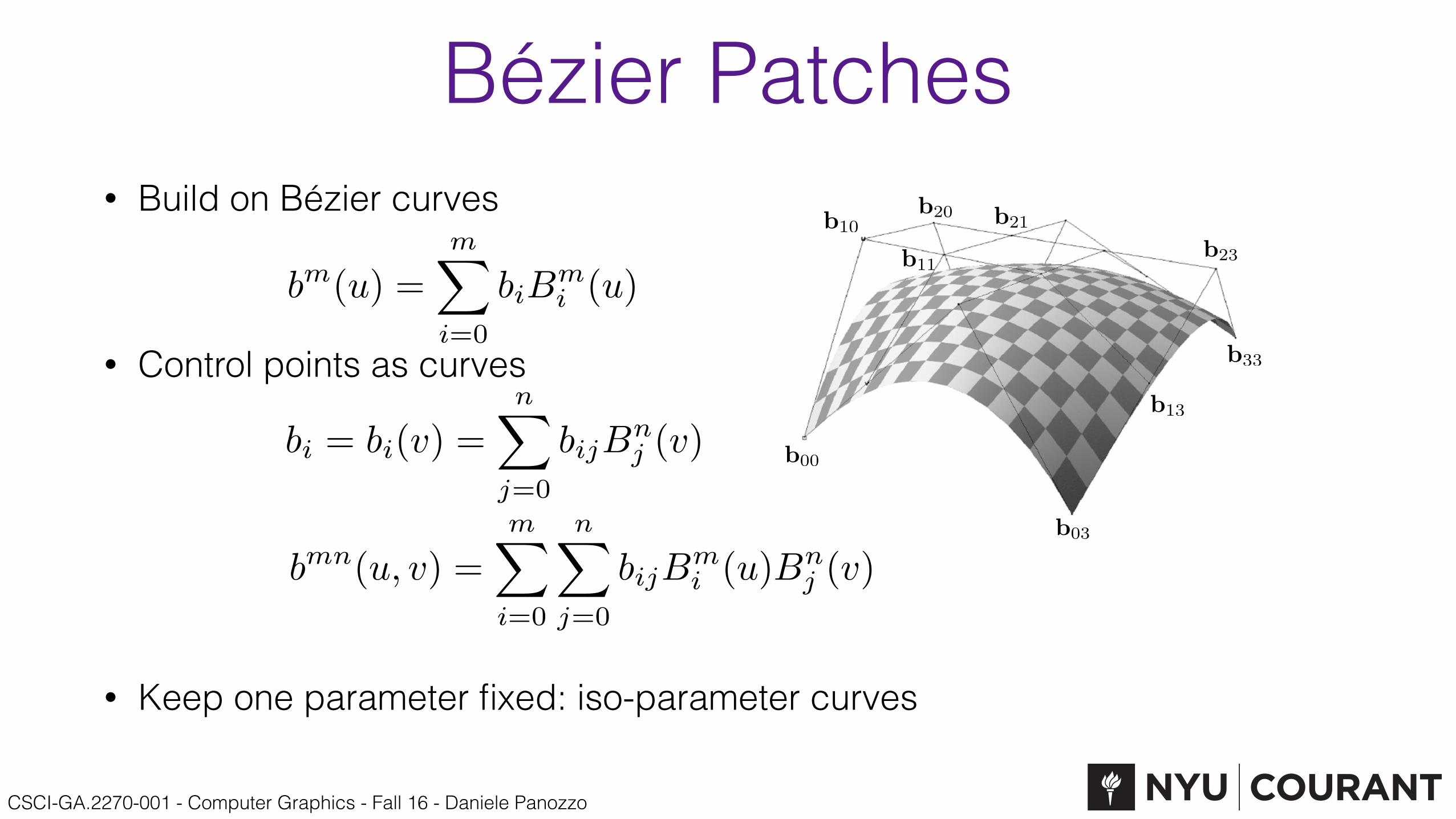
Bézier Patches• Build on Bézier curves
• Control points as curves
• Keep one parameter fixed: iso-parameter curves
bm(u) =mX
i=0
biBmi (u)
bi = bi(v) =nX
j=0
bijBnj (v)
bmn(u, v) =mX
i=0
nX
j=0
bijBmi (u)Bn
j (v)

CSCI-GA.2270-001 - Computer Graphics - Fall 16 - Daniele Panozzo
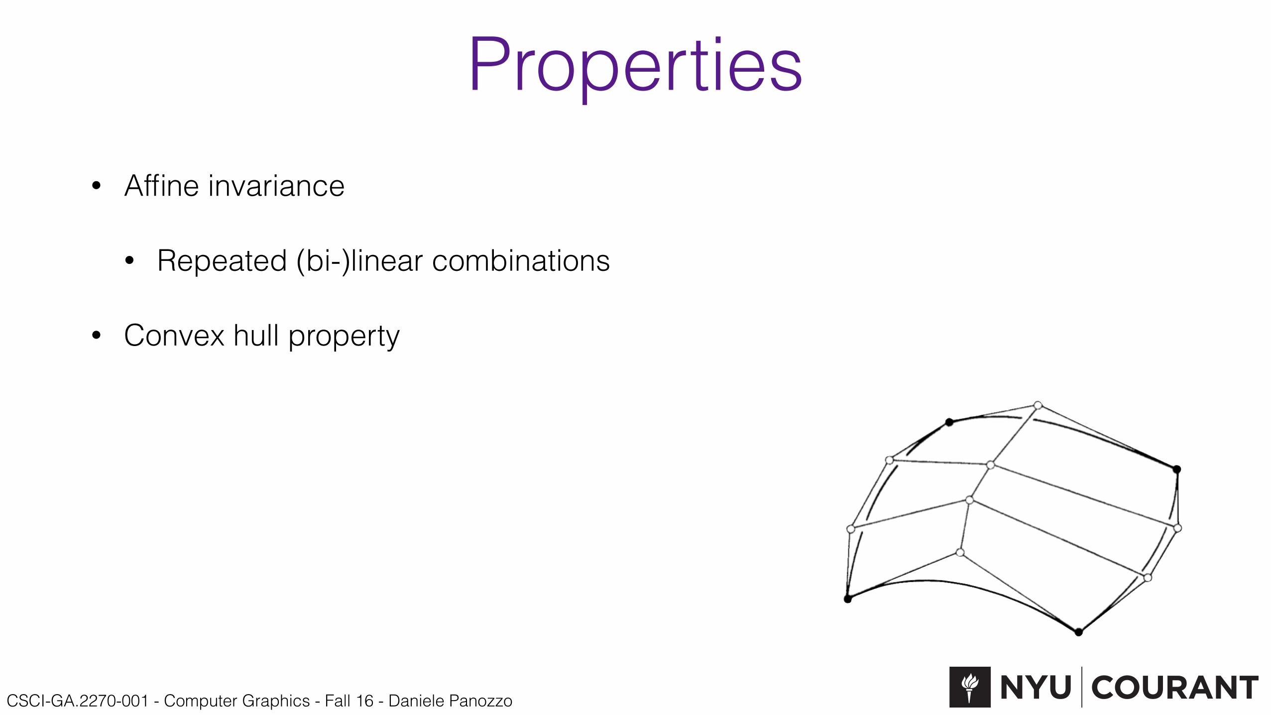
Properties• Affine invariance
CSCI-GA.2270-001 - Computer Graphics - Fall 16 - Daniele Panozzo
Properties• Affine invariance
• Repeated (bi-)linear combinations
• Convex hull property

CSCI-GA.2270-001 - Computer Graphics - Fall 16 - Daniele Panozzo
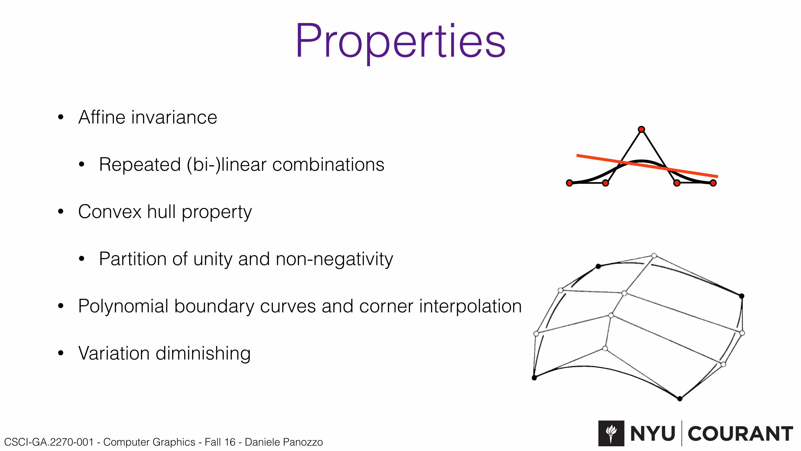
Properties• Affine invariance
• Repeated (bi-)linear combinations
• Convex hull property
• Partition of unity and non-negativity
• Polynomial boundary curves and corner interpolation
CSCI-GA.2270-001 - Computer Graphics - Fall 16 - Daniele Panozzo
Properties• Affine invariance
• Repeated (bi-)linear combinations
• Convex hull property
• Partition of unity and non-negativity
• Polynomial boundary curves and corner interpolation
• Variation diminishing
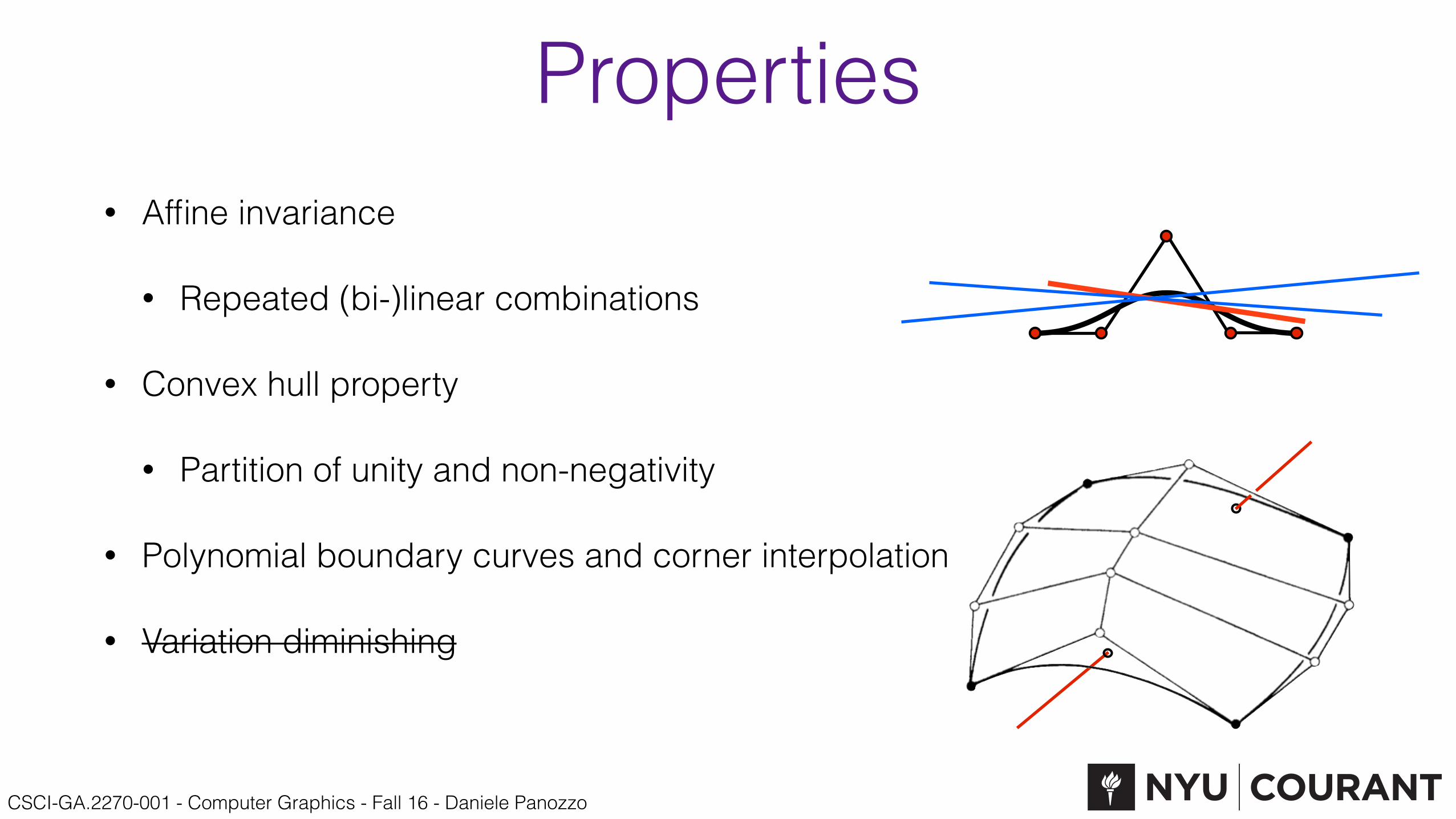
CSCI-GA.2270-001 - Computer Graphics - Fall 16 - Daniele Panozzo
Properties• Affine invariance
• Repeated (bi-)linear combinations
• Convex hull property
• Partition of unity and non-negativity
• Polynomial boundary curves and corner interpolation
• Variation diminishing
CSCI-GA.2270-001 - Computer Graphics - Fall 16 - Daniele Panozzo
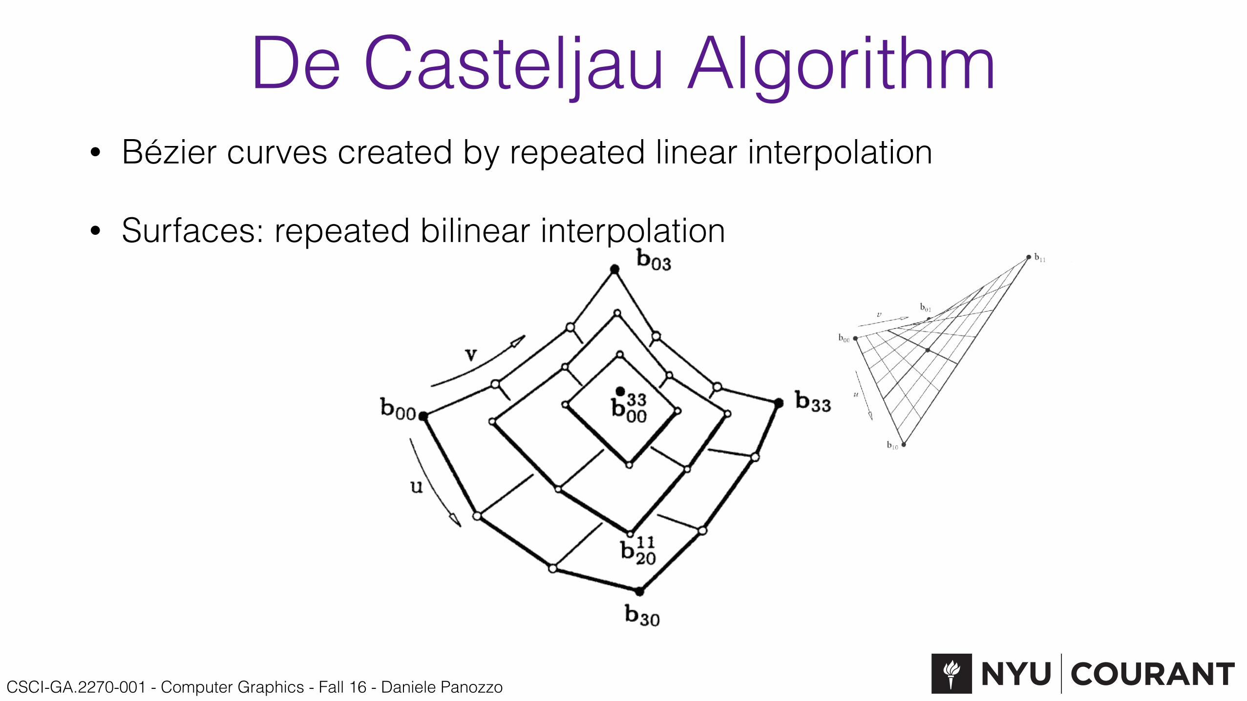
De Casteljau Algorithm• Bézier curves created by repeated linear interpolation
• Surfaces: repeated bilinear interpolation
CSCI-GA.2270-001 - Computer Graphics - Fall 16 - Daniele Panozzo
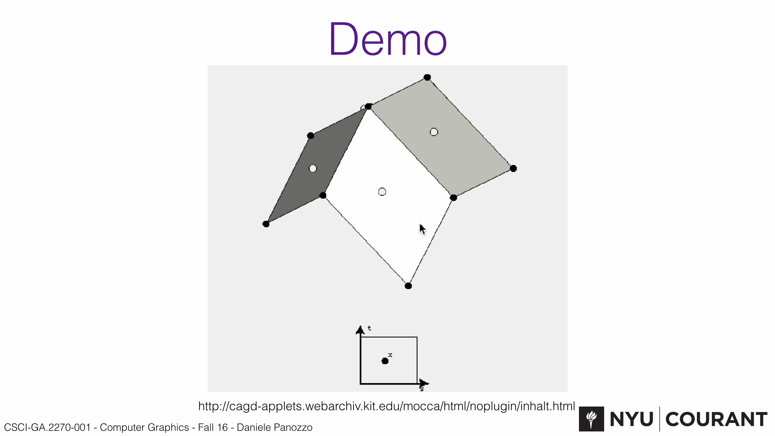
Demo
http://cagd-applets.webarchiv.kit.edu/mocca/html/noplugin/inhalt.html
CSCI-GA.2270-001 - Computer Graphics - Fall 16 - Daniele Panozzo
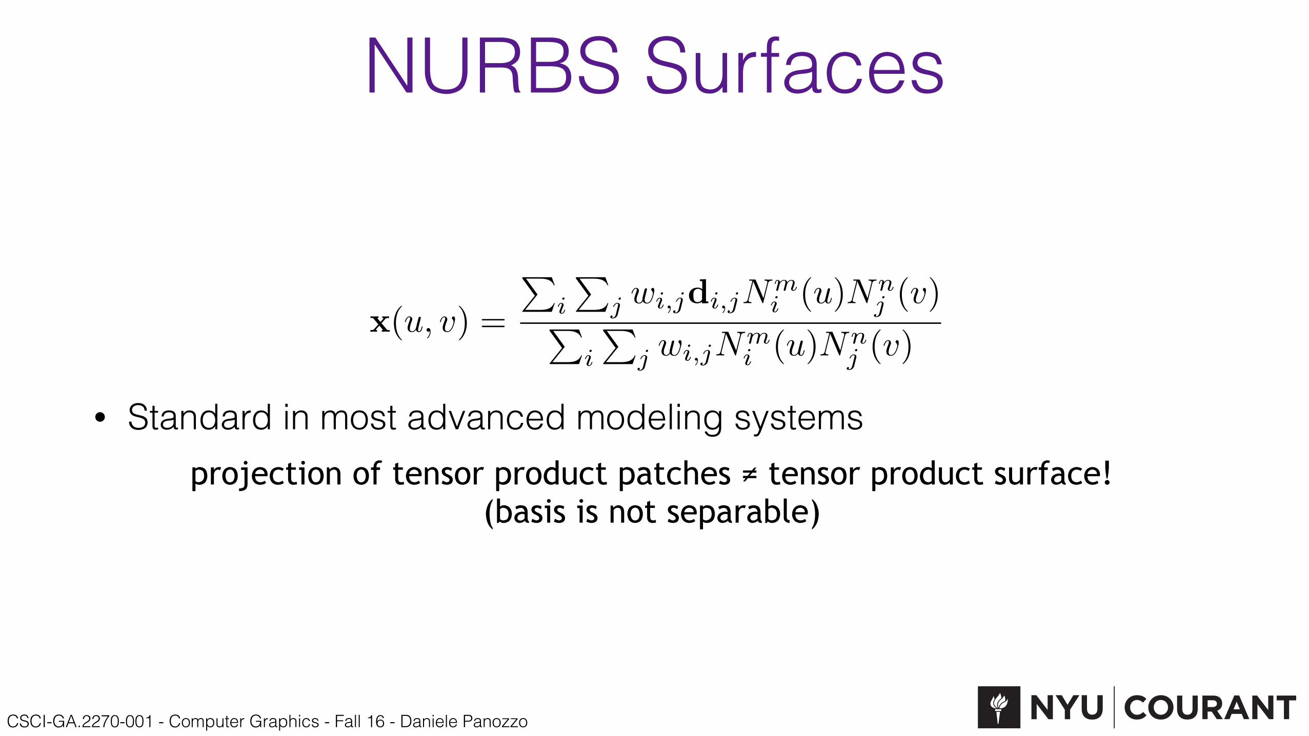
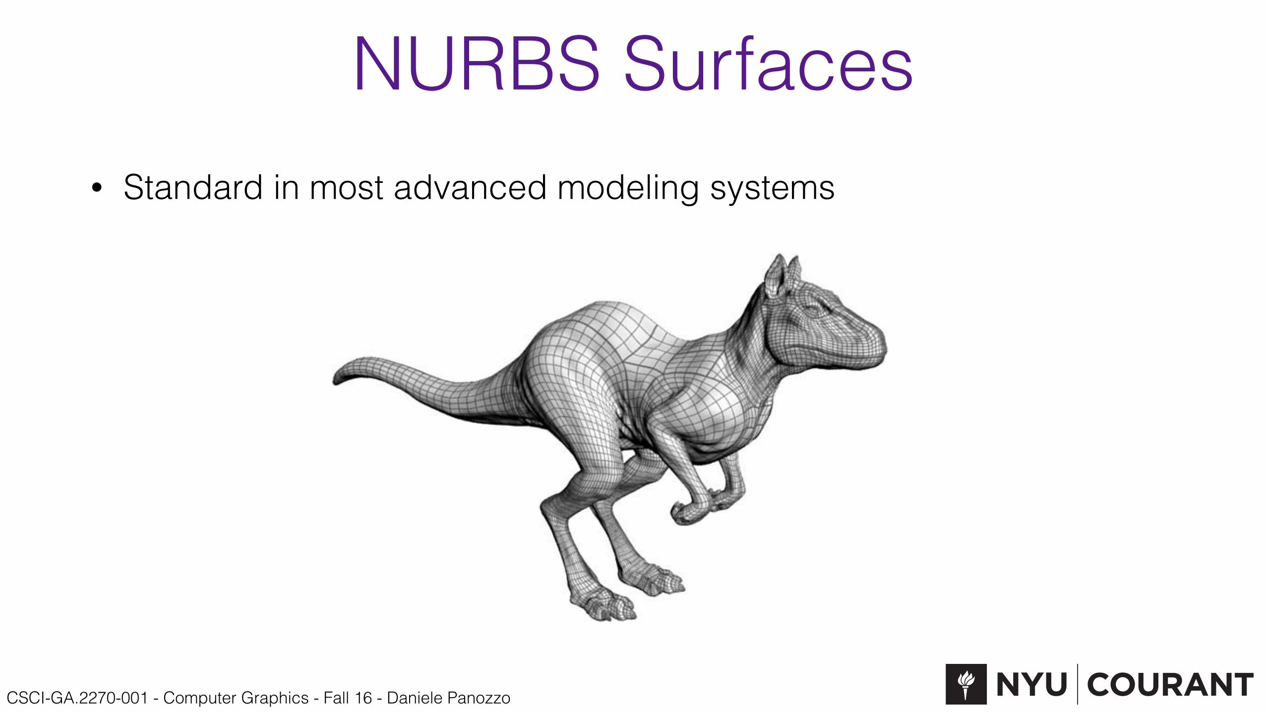
NURBS Surfaces
• Standard in most advanced modeling systems
x(u, v) =
!i
!j wi,jdi,jN
mi (u)Nn
j (v)!
i
!j wi,jN
mi (u)Nn
j (v)
projection of tensor product patches ≠ tensor product surface! (basis is not separable)
CSCI-GA.2270-001 - Computer Graphics - Fall 16 - Daniele Panozzo
NURBS Surfaces• Standard in most advanced modeling systems

CSCI-GA.2270-001 - Computer Graphics - Fall 16 - Daniele Panozzo
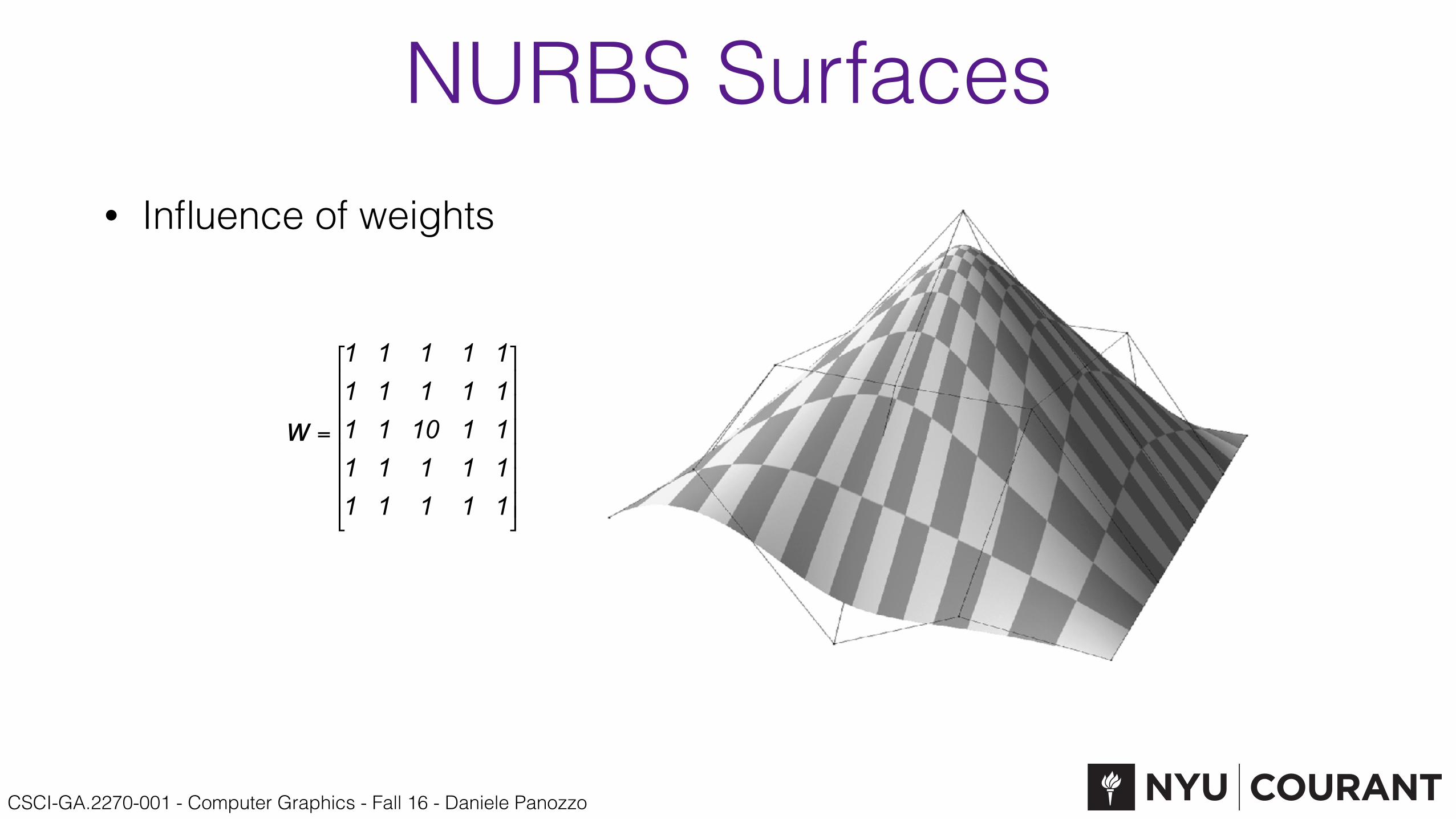
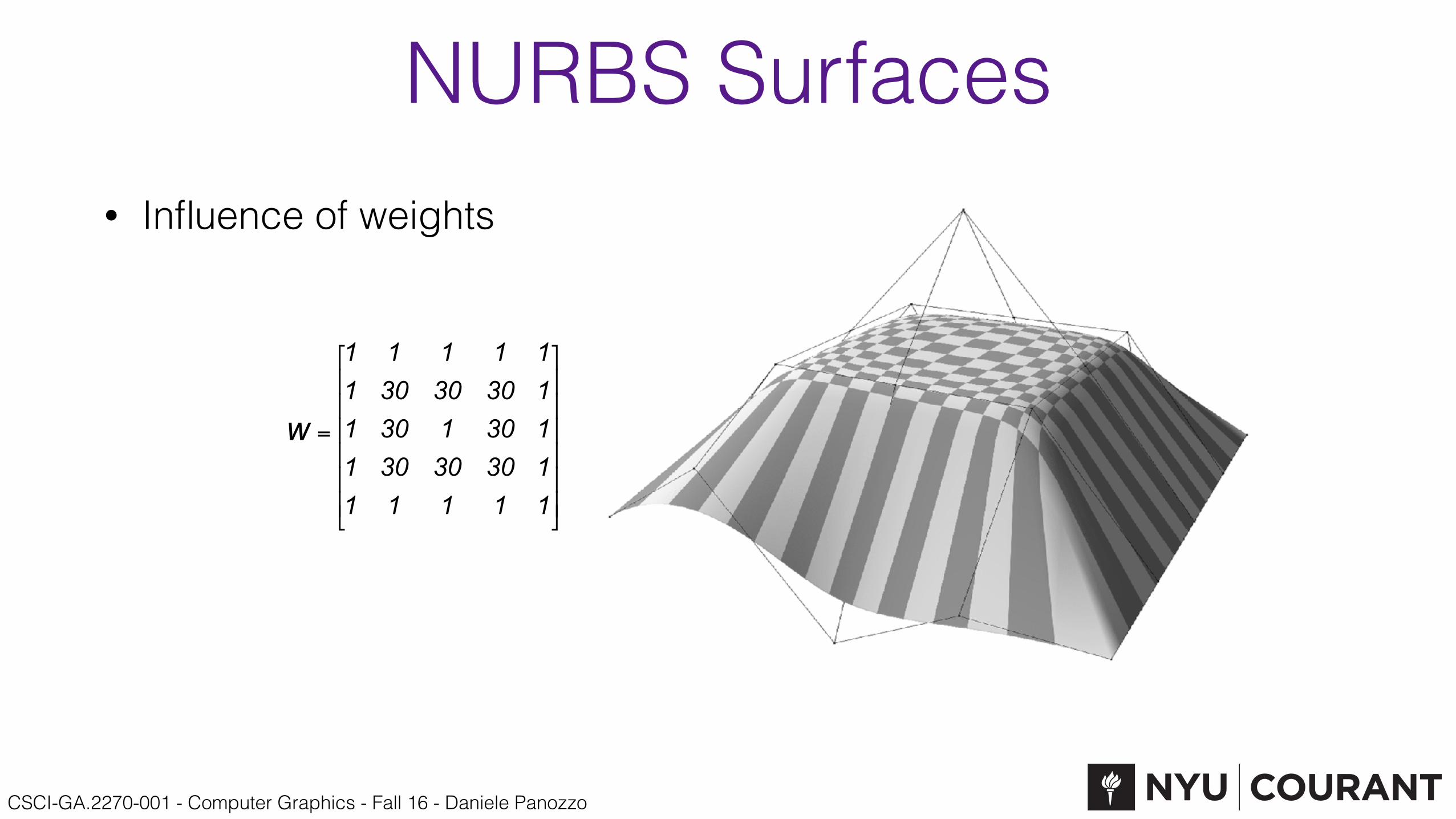
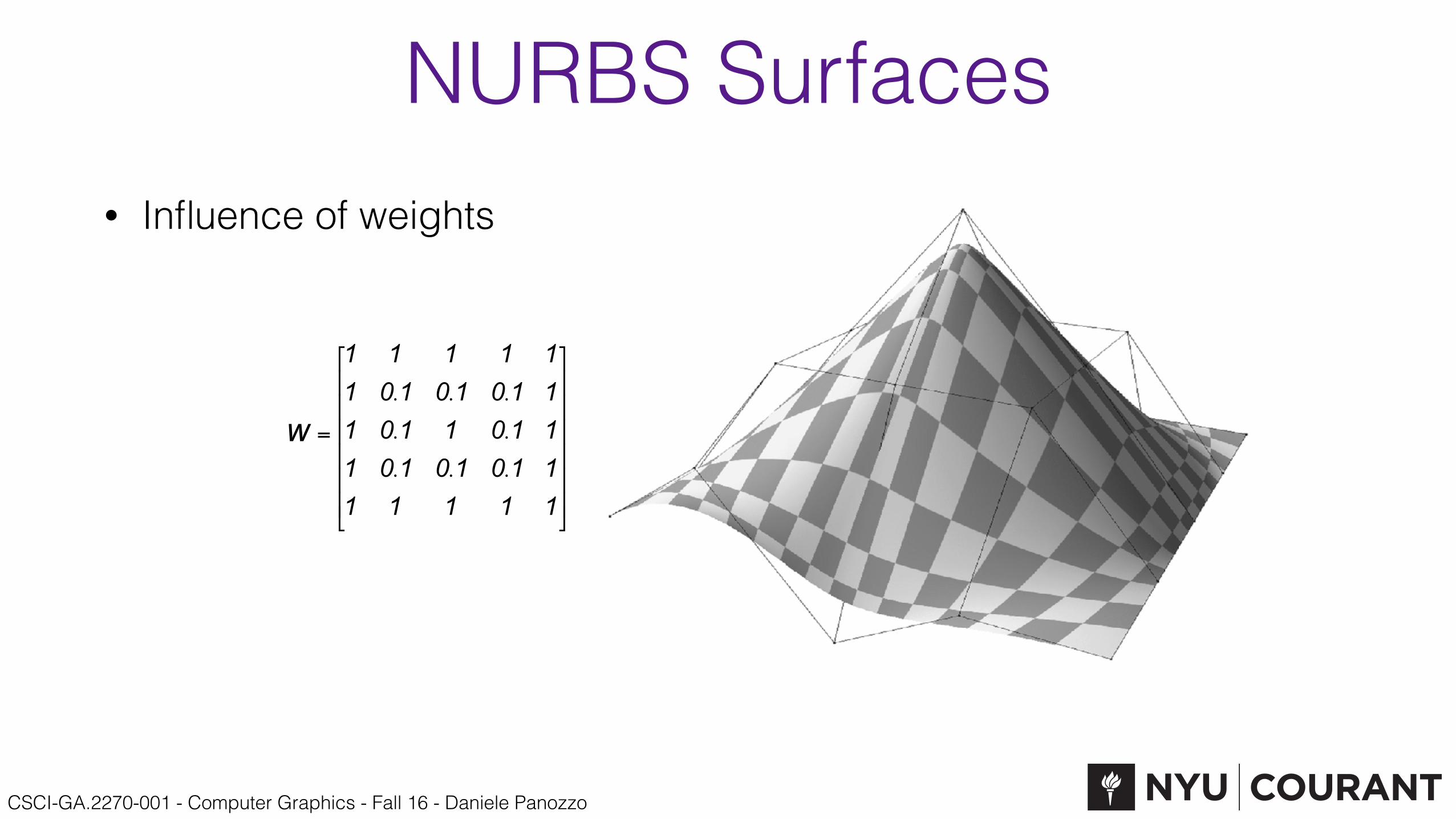
NURBS Surfaces• Influence of weights
CSCI-GA.2270-001 - Computer Graphics - Fall 16 - Daniele Panozzo
NURBS Surfaces• Influence of weights
CSCI-GA.2270-001 - Computer Graphics - Fall 16 - Daniele Panozzo
NURBS Surfaces• Influence of weights
CSCI-GA.2270-001 - Computer Graphics - Fall 16 - Daniele Panozzo
NURBS Surfaces• Influence of weights
CSCI-GA.2270-001 - Computer Graphics - Fall 16 - Daniele Panozzo
Subdivision Surfaces

CSCI-GA.2270-001 - Computer Graphics - Fall 16 - Daniele Panozzo
Why?• Tensor product surfaces are defined on “regular grids”
• They cannot be defined on arbitrary meshes
CSCI-GA.2270-001 - Computer Graphics - Fall 16 - Daniele Panozzo
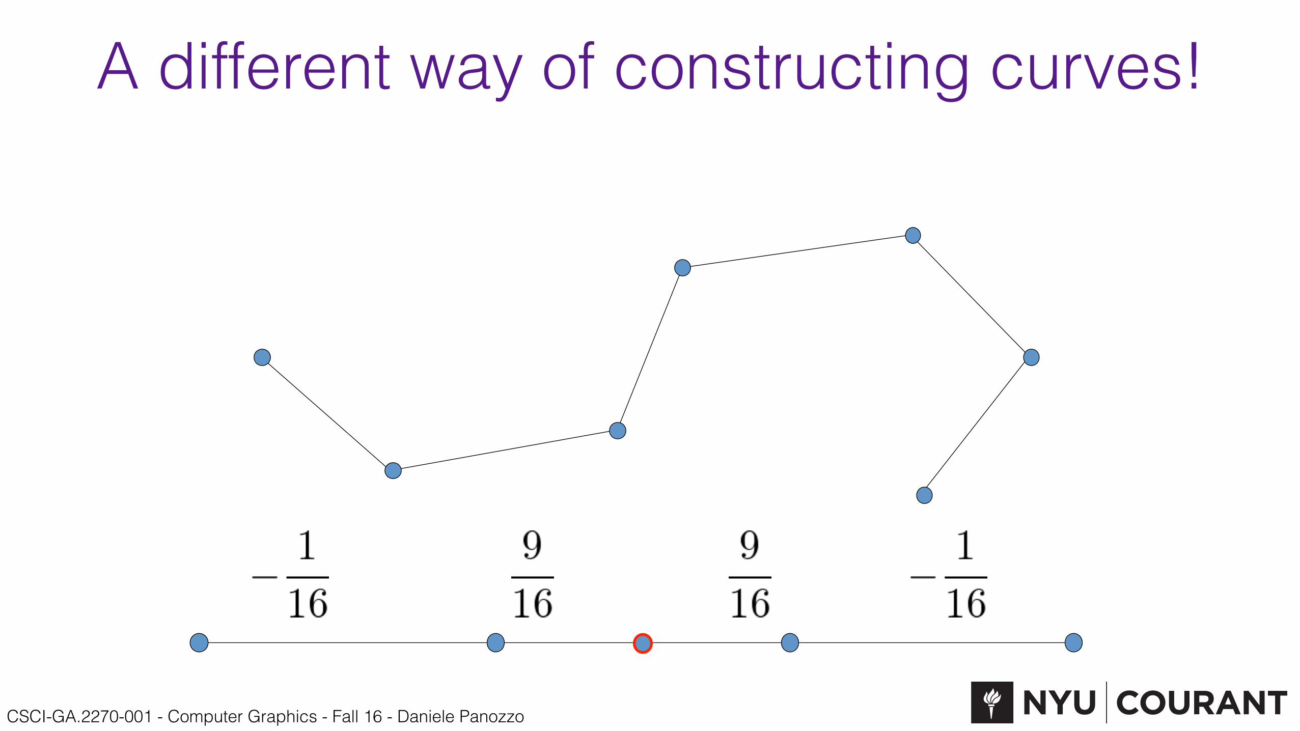
A different way of constructing curves!

CSCI-GA.2270-001 - Computer Graphics - Fall 16 - Daniele Panozzo
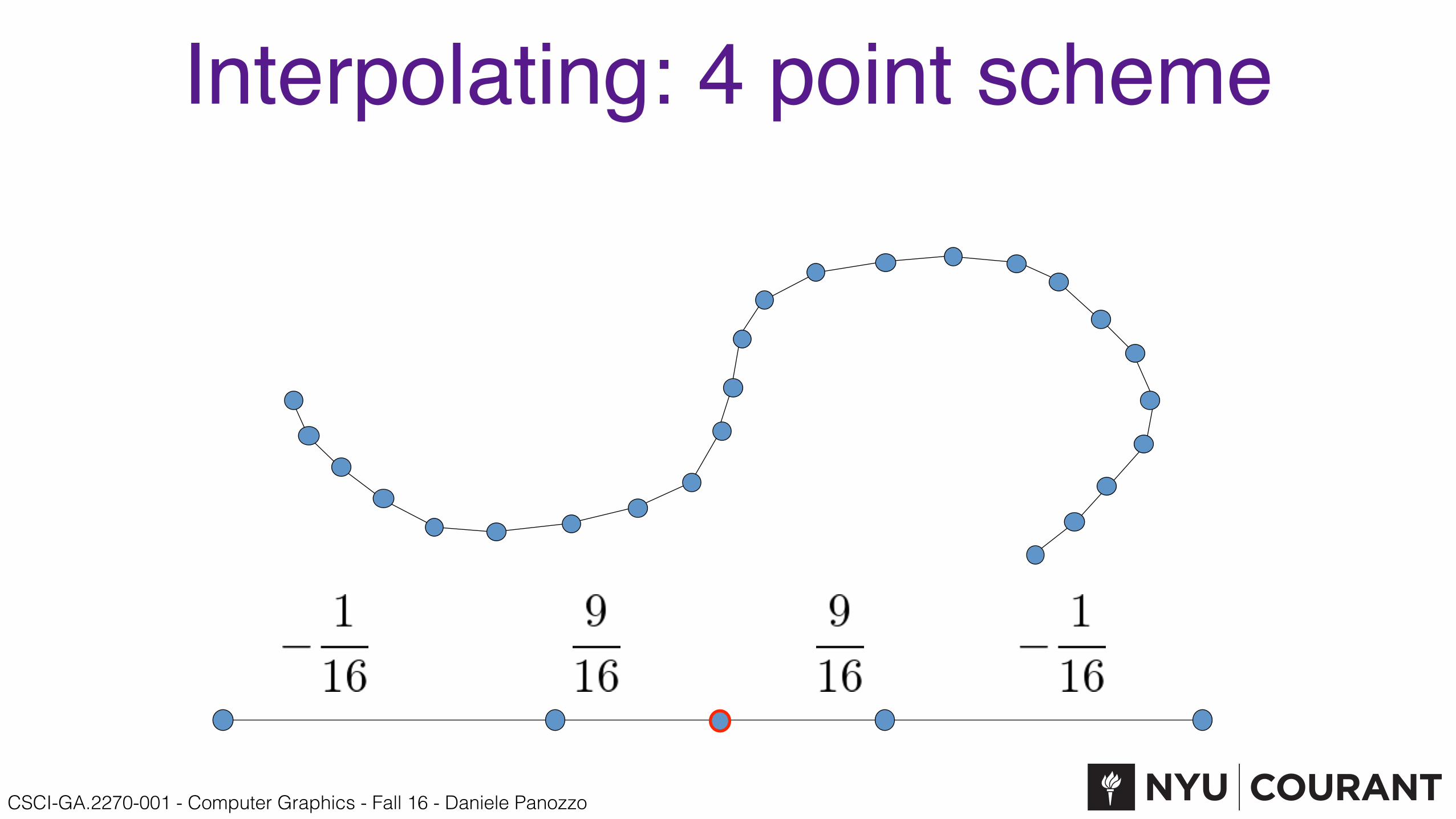
Interpolating: 4 point scheme
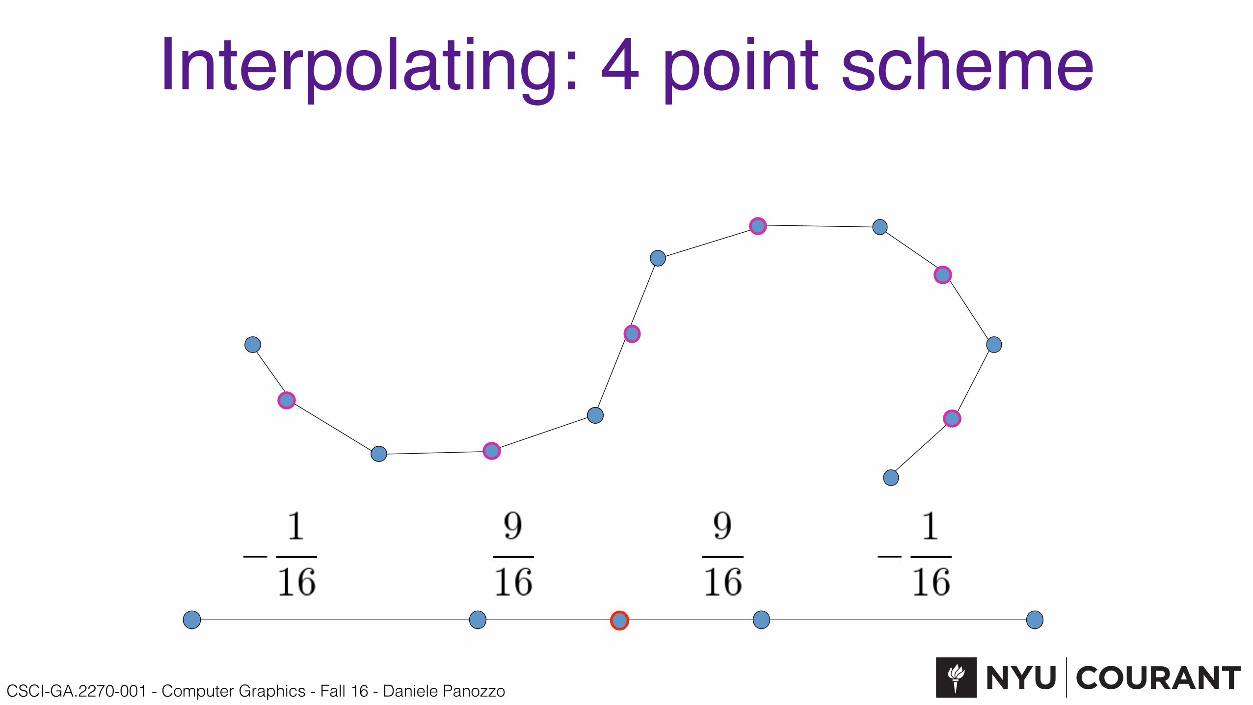
CSCI-GA.2270-001 - Computer Graphics - Fall 16 - Daniele Panozzo
Interpolating: 4 point scheme
CSCI-GA.2270-001 - Computer Graphics - Fall 16 - Daniele Panozzo
Interpolating: 4 point scheme
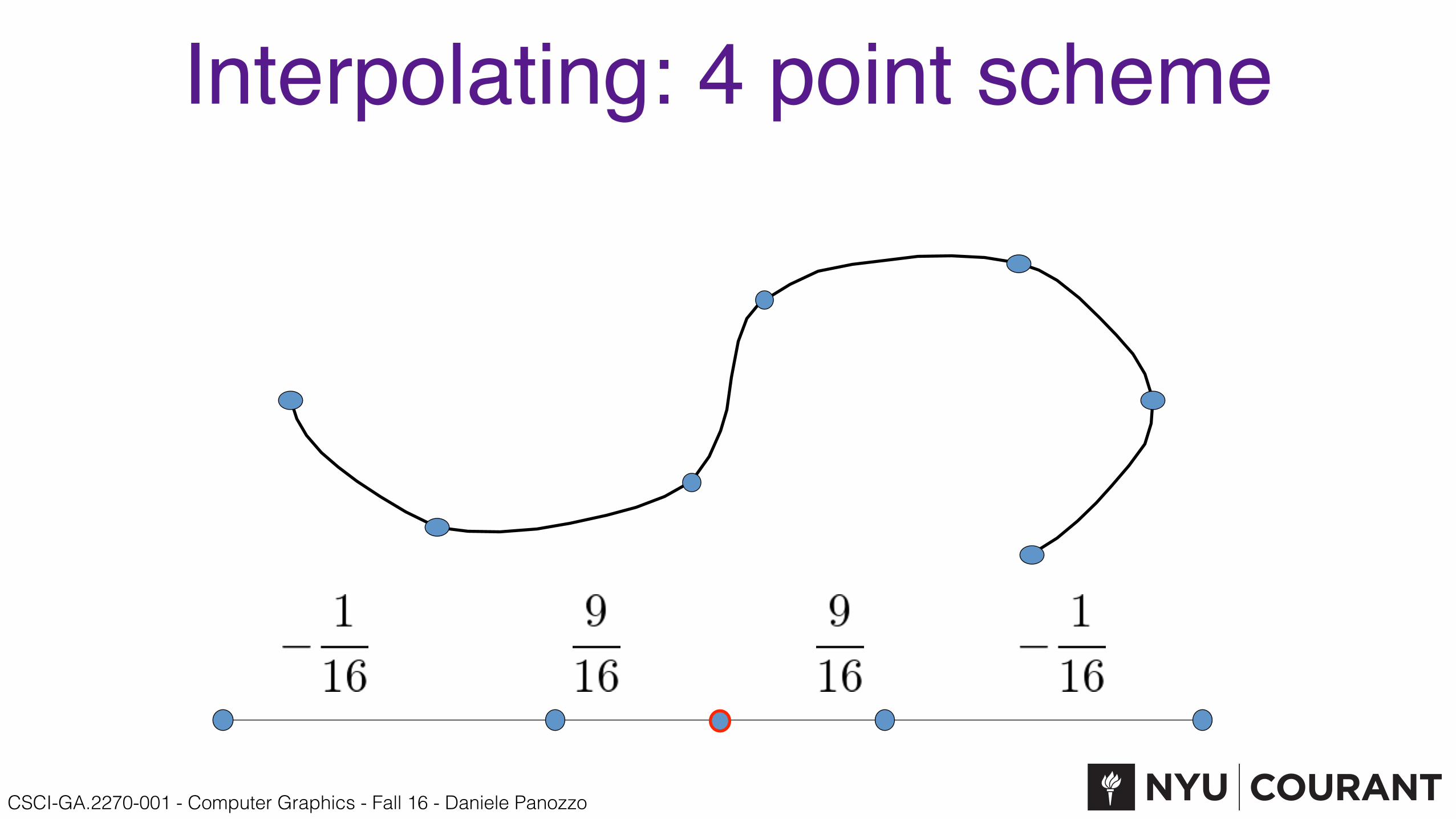
CSCI-GA.2270-001 - Computer Graphics - Fall 16 - Daniele Panozzo
Interpolating: 4 point scheme
CSCI-GA.2270-001 - Computer Graphics - Fall 16 - Daniele Panozzo
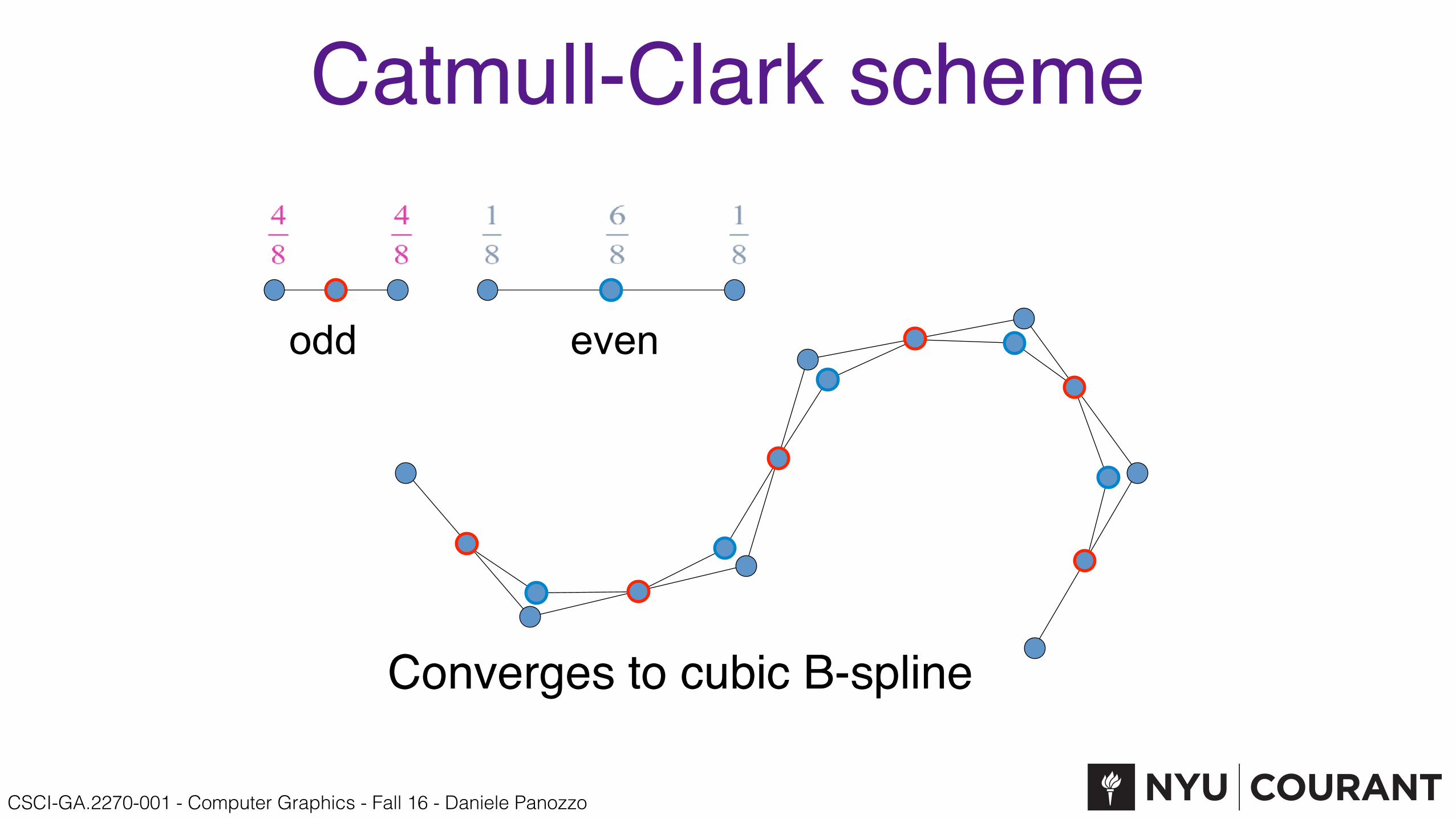
Catmull-Clark scheme
evenodd
Converges to cubic B-spline
CSCI-GA.2270-001 - Computer Graphics - Fall 16 - Daniele Panozzo
Subdivision Methods• Principal characteristics:
• triangular or quadrangular meshes
• approximating or interpolating
• smoothness of the limit surface
• We will study 2 of them:
• Loop subdivision for triangle meshes (Approximating, C2)
• Catmull-Clark subdivision for quadrilateral meshes (Approximating, C2)
• Other famous schemes (see the references for details)
• Butterfly, Kobbelt, Doo-Sabin, Midedge, Biquartic
CSCI-GA.2270-001 - Computer Graphics - Fall 16 - Daniele Panozzo
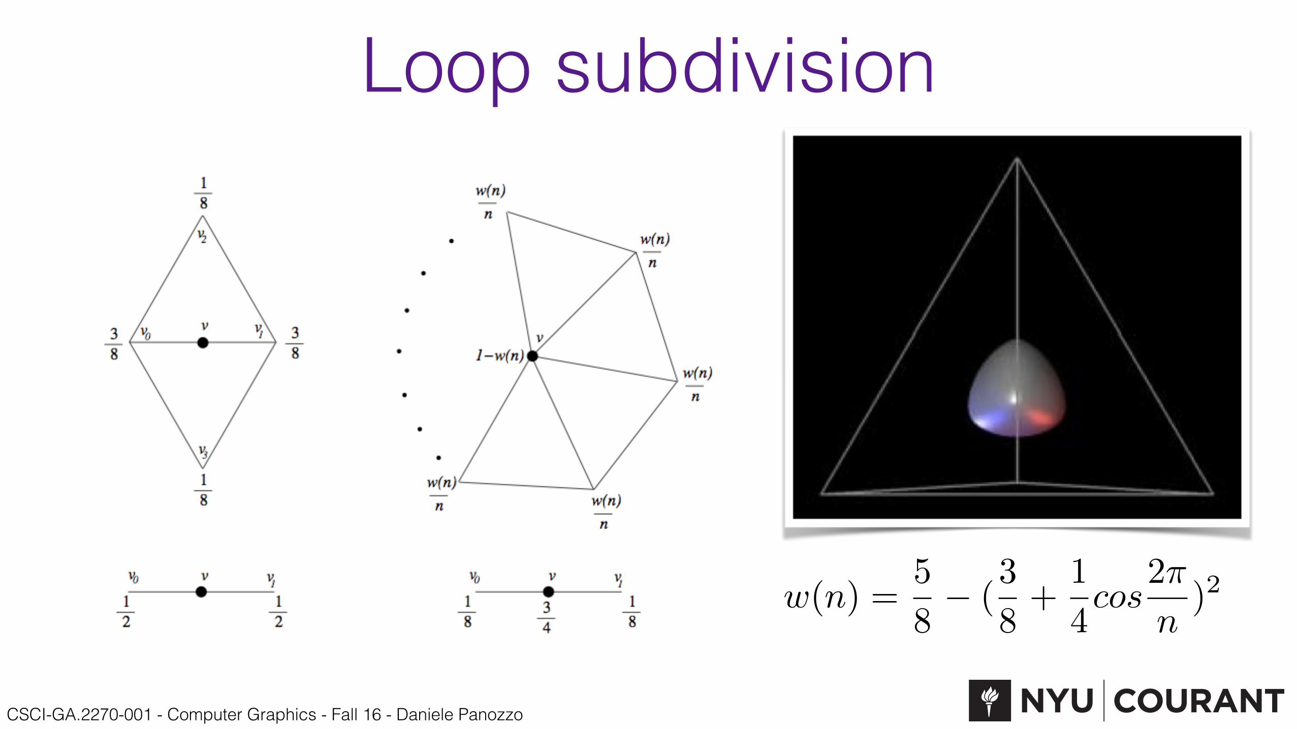
Loop subdivision
w(n) =5
8� (
3
8+
1
4cos
2⇡
n
)2
CSCI-GA.2270-001 - Computer Graphics - Fall 16 - Daniele Panozzo
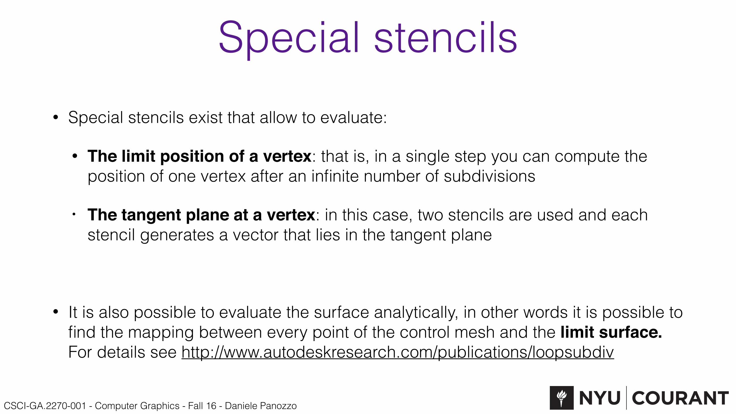
Special stencils• Special stencils exist that allow to evaluate:
• The limit position of a vertex: that is, in a single step you can compute the position of one vertex after an infinite number of subdivisions
• The tangent plane at a vertex: in this case, two stencils are used and each stencil generates a vector that lies in the tangent plane
• It is also possible to evaluate the surface analytically, in other words it is possible to find the mapping between every point of the control mesh and the limit surface. For details see http://www.autodeskresearch.com/publications/loopsubdiv
CSCI-GA.2270-001 - Computer Graphics - Fall 16 - Daniele Panozzo
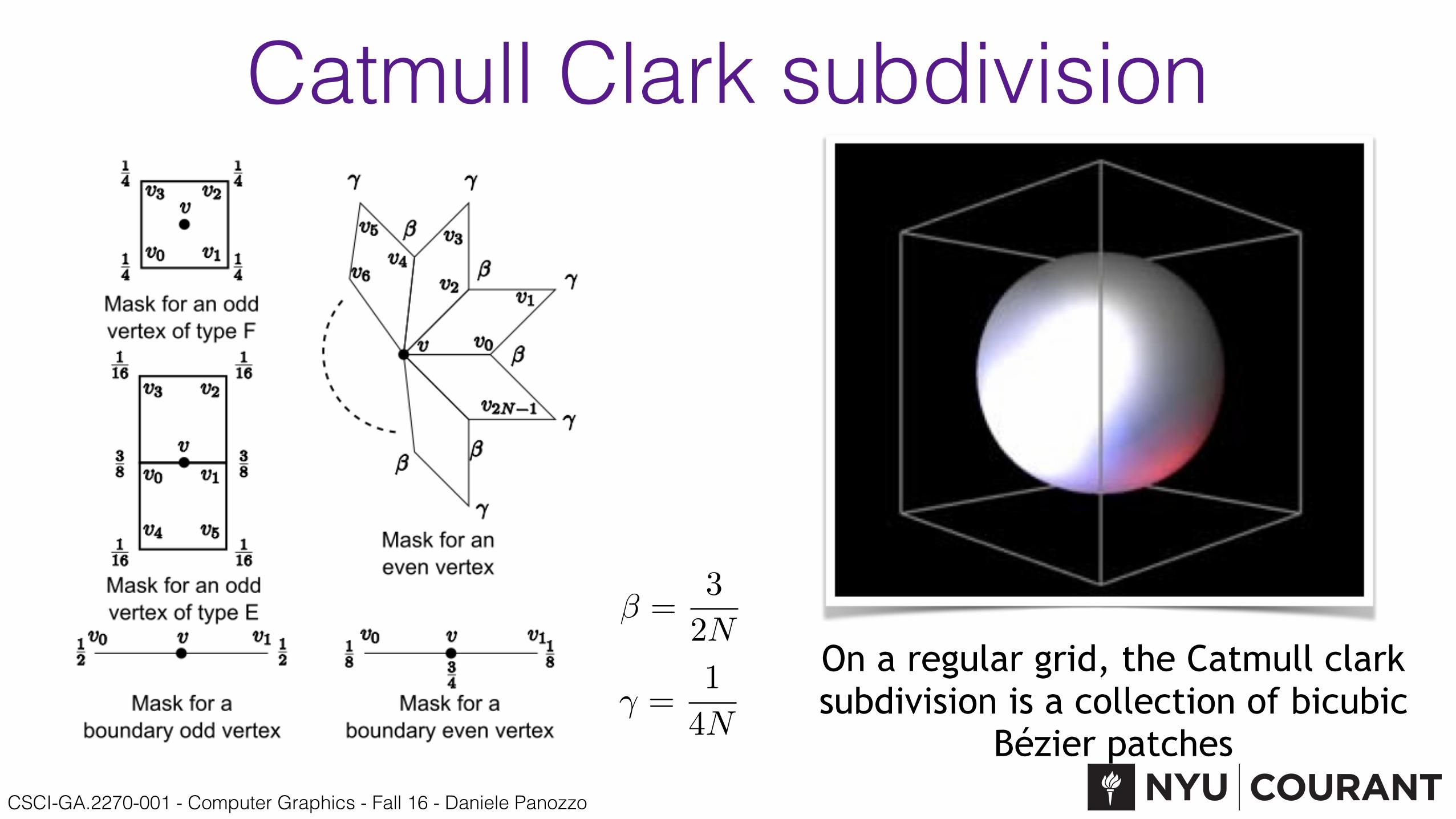
Catmull Clark subdivision
� =3
2N
� =1
4N
On a regular grid, the Catmull clark subdivision is a collection of bicubic
Bézier patches

CSCI-GA.2270-001 - Computer Graphics - Fall 16 - Daniele Panozzo
Catmull-Clark• It is the standard in the animation industry
• All the major 3D modeling softwares support it
• Similarly to Loop:
• stencils for the limit surface
• stencils for tangent plane
• it can be evaluated analytically

CSCI-GA.2270-001 - Computer Graphics - Fall 16 - Daniele Panozzo
How are they used in practice?
CSCI-GA.2270-001 - Computer Graphics - Fall 16 - Daniele Panozzo
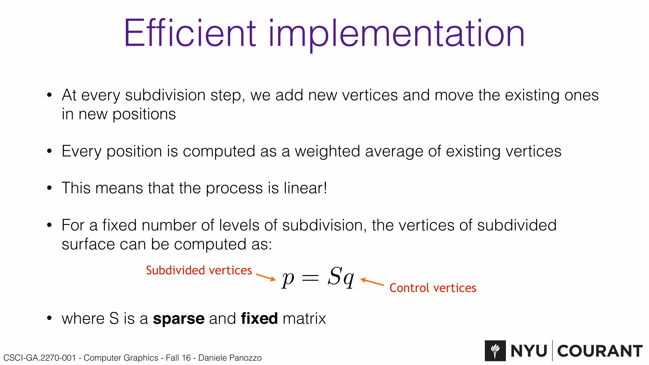
Efficient implementation• At every subdivision step, we add new vertices and move the existing ones
in new positions
• Every position is computed as a weighted average of existing vertices
• This means that the process is linear!
• For a fixed number of levels of subdivision, the vertices of subdivided surface can be computed as:
• where S is a sparse and fixed matrix
p = SqSubdivided verticesControl vertices

CSCI-GA.2270-001 - Computer Graphics - Fall 16 - Daniele Panozzo
T-spline
• Extension of splines for non-rectangular grids
• http://www.youtube.com/watch?v=k1ro9S-cAwI
CSCI-GA.2270-001 - Computer Graphics - Fall 16 - Daniele Panozzo
References
Fundamentals of Computer Graphics, Fourth Edition 4th Edition by Steve Marschner, Peter Shirley
Chapter 15
Curves and Surfaces for CAGD - Gerald Farin
Subdivision Zoo - Denis Zorin http://www.cmlab.csie.ntu.edu.tw/~robin/courses/gm/note/subdivision-prn.pdf
CSCI-GA.2270-001 - Computer Graphics - Fall 16 - Daniele Panozzo
Projective Transformations
CSCI-GA.2270-001 - Computer Graphics - Fall 16 - Daniele Panozzo
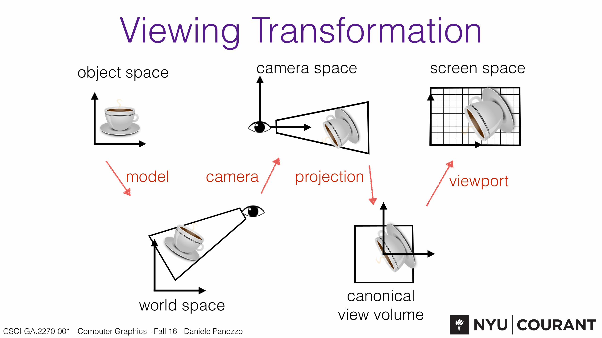
Viewing Transformationobject space
model camera projection viewport
canonical view volumeworld space
camera space screen space
CSCI-GA.2270-001 - Computer Graphics - Fall 16 - Daniele Panozzo
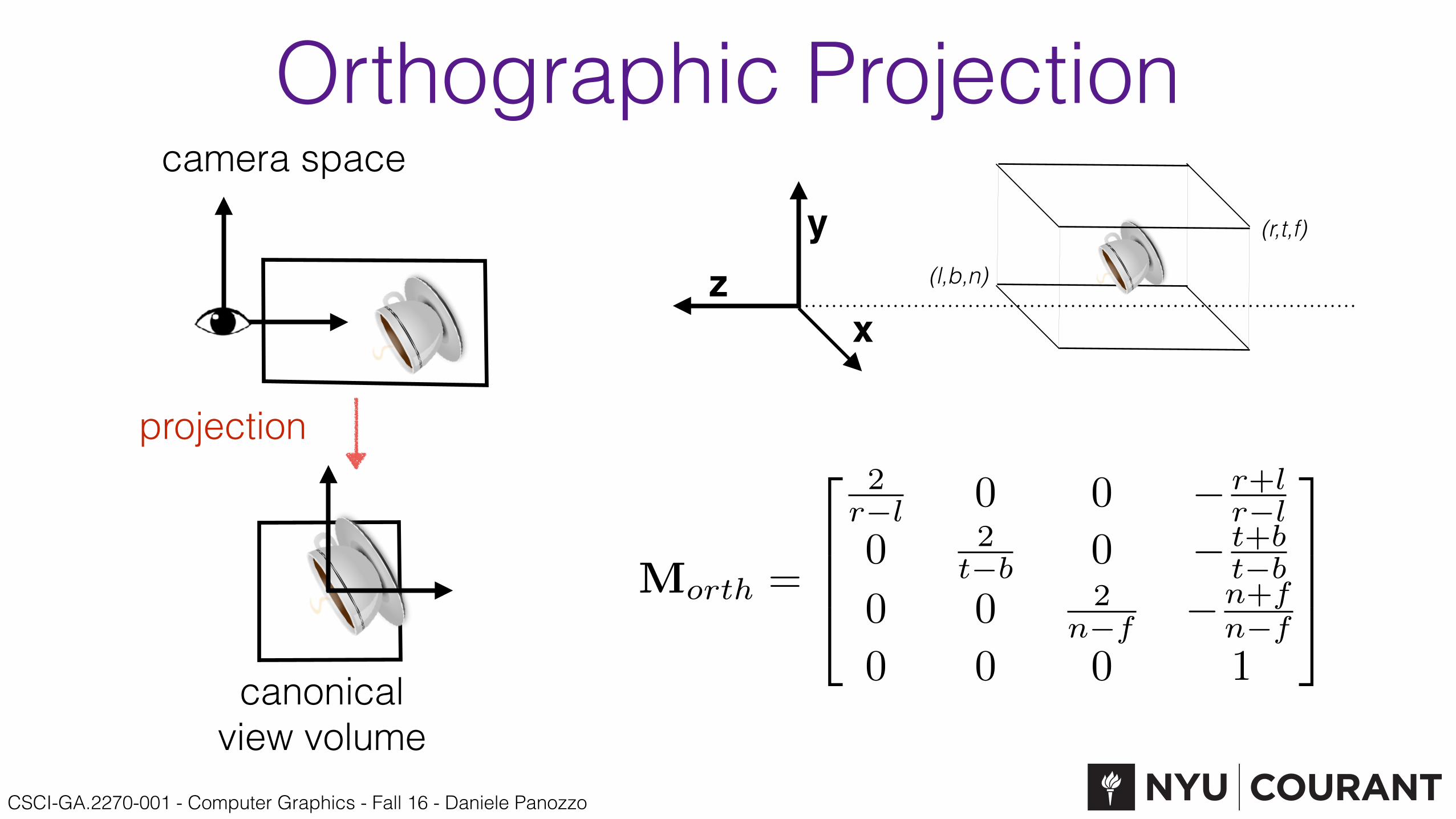
Orthographic Projection
projection
canonical view volume
camera space
xz
y(l,b,n)
(r,t,f)
Morth
=
2
664
2r�l
0 0 � r+l
r�l
0 2t�b
0 � t+b
t�b
0 0 2n�f
�n+f
n�f
0 0 0 1
3
775
CSCI-GA.2270-001 - Computer Graphics - Fall 16 - Daniele Panozzo
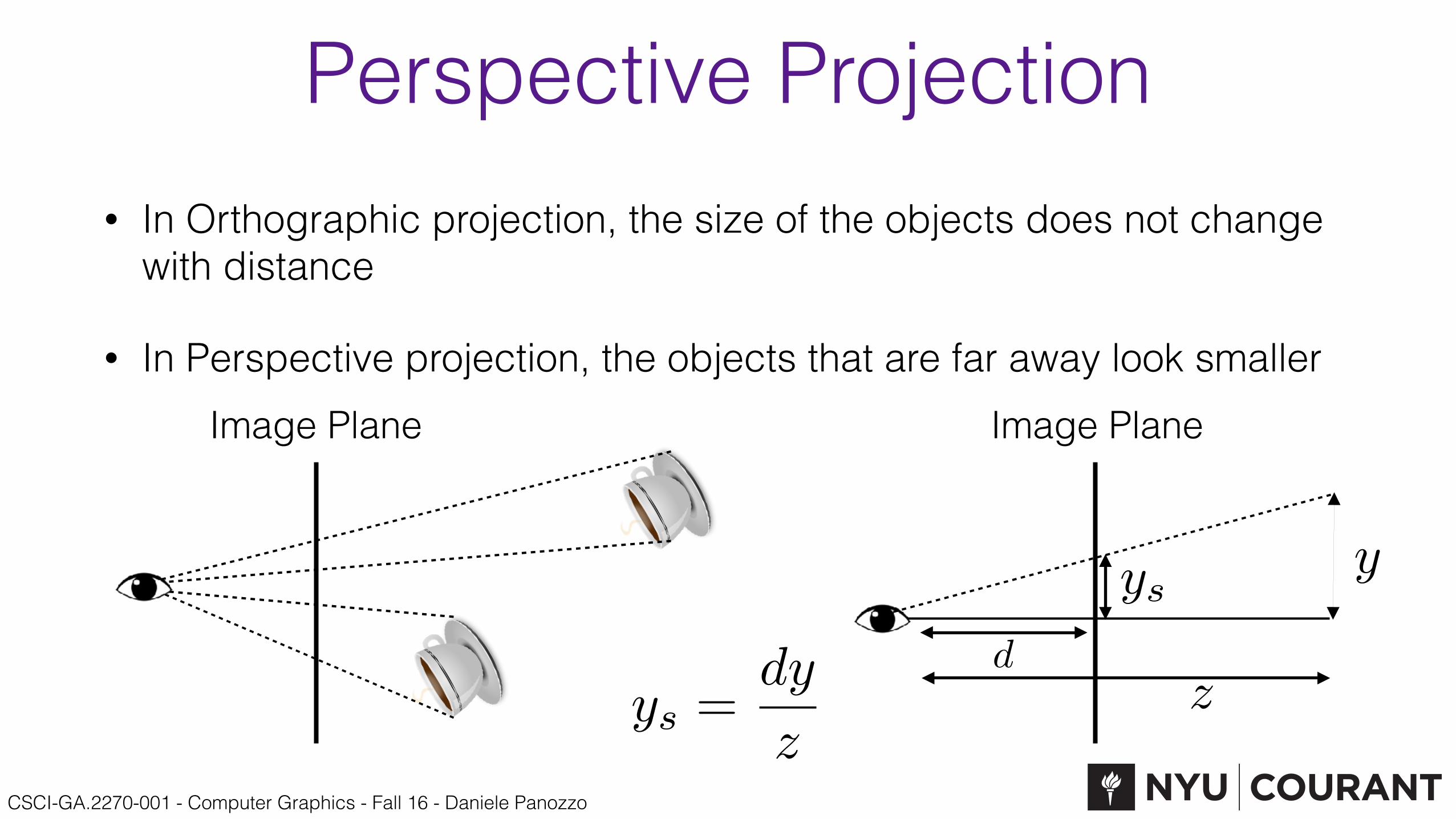
Perspective Projection• In Orthographic projection, the size of the objects does not change
with distance
• In Perspective projection, the objects that are far away look smallerImage Plane
ysy
dzys =
dy
z
Image Plane
CSCI-GA.2270-001 - Computer Graphics - Fall 16 - Daniele Panozzo
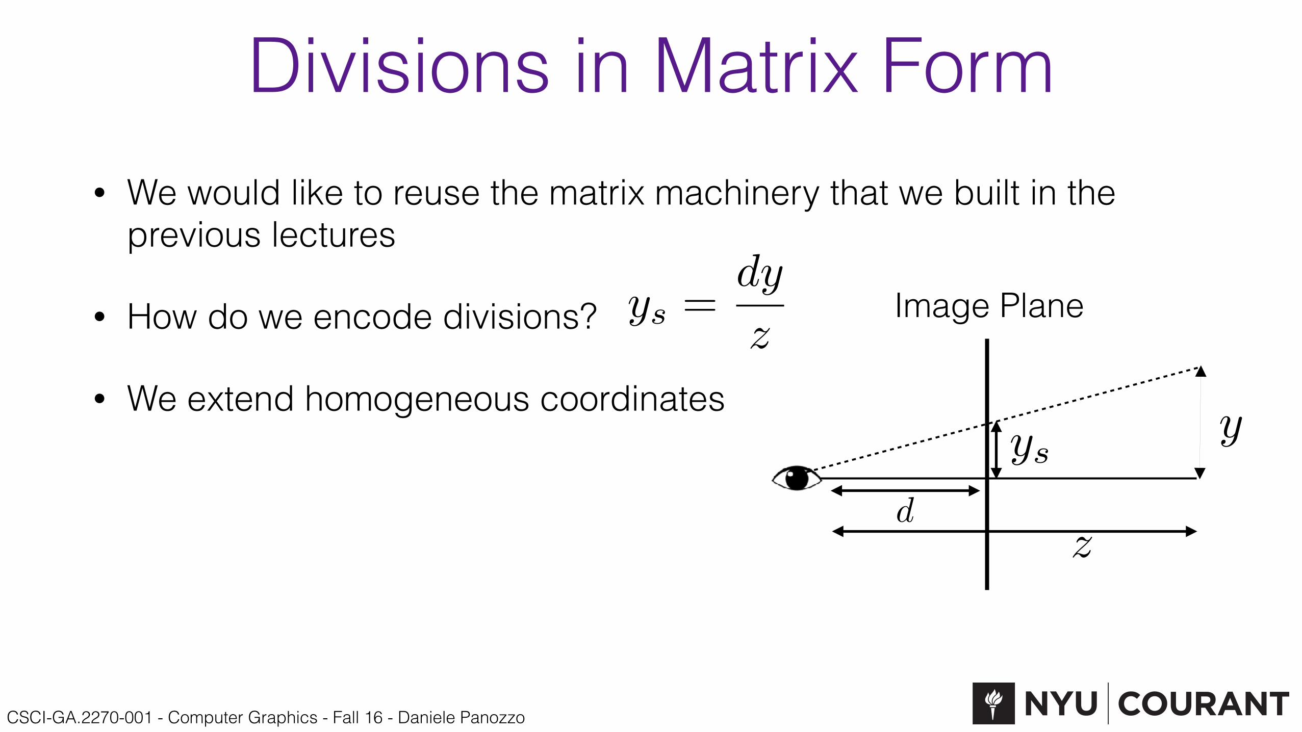
Divisions in Matrix Form• We would like to reuse the matrix machinery that we built in the
previous lectures
• How do we encode divisions?
• We extend homogeneous coordinatesys
y
dz
ys =dy
zImage Plane

CSCI-GA.2270-001 - Computer Graphics - Fall 16 - Daniele Panozzo
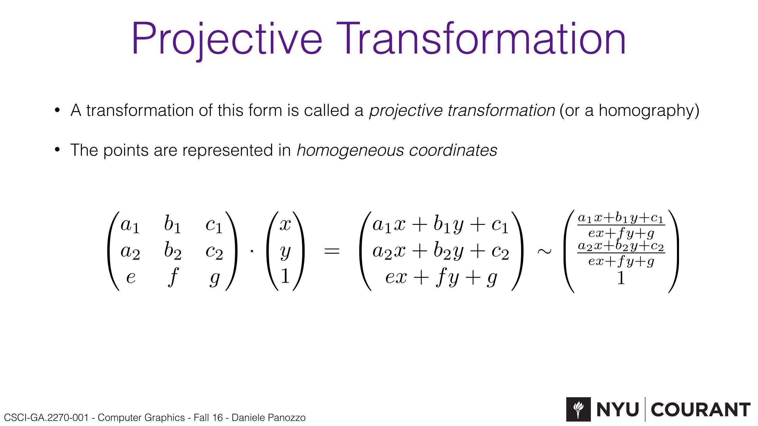
• What do we have left?
• We can use the last row of the transformation:
Until now…
0
@a1 b1 c1
a2 b2 c2
0 0 1
1
A ·
0
@x
y
1
1
A =
0
@a1x+ b1y + c1
a2x+ b2y + c2
1
1
A
0
@a1 b1 c1
a2 b2 c2
e f g
1
A ·
0
@x
y
1
1
A =
0
@a1x+ b1y + c1
a2x+ b2y + c2
ex+ fy + g
1
A⇠
0
B@
a1x+b1y+c1
ex+fy+g
a2x+b2y+c2
ex+fy+g
1
1
CA

CSCI-GA.2270-001 - Computer Graphics - Fall 16 - Daniele Panozzo
Intuition• Purely algebraic:
• Or as a projection, where each line is identified by a point on the plane z=1
• Note that in this case, you can think of it as a transformation in a space with one more dimension
0
@x
y
w
1
A ⇠
0
@x/w
y/w
1
1
A
CSCI-GA.2270-001 - Computer Graphics - Fall 16 - Daniele Panozzo
Projective Transformation• A transformation of this form is called a projective transformation (or a homography)
• The points are represented in homogeneous coordinates
0
@a1 b1 c1
a2 b2 c2
e f g
1
A ·
0
@x
y
1
1
A =
0
@a1x+ b1y + c1
a2x+ b2y + c2
ex+ fy + g
1
A ⇠
0
B@
a1x+b1y+c1
ex+fy+g
a2x+b2y+c2
ex+fy+g
1
1
CA
CSCI-GA.2270-001 - Computer Graphics - Fall 16 - Daniele Panozzo
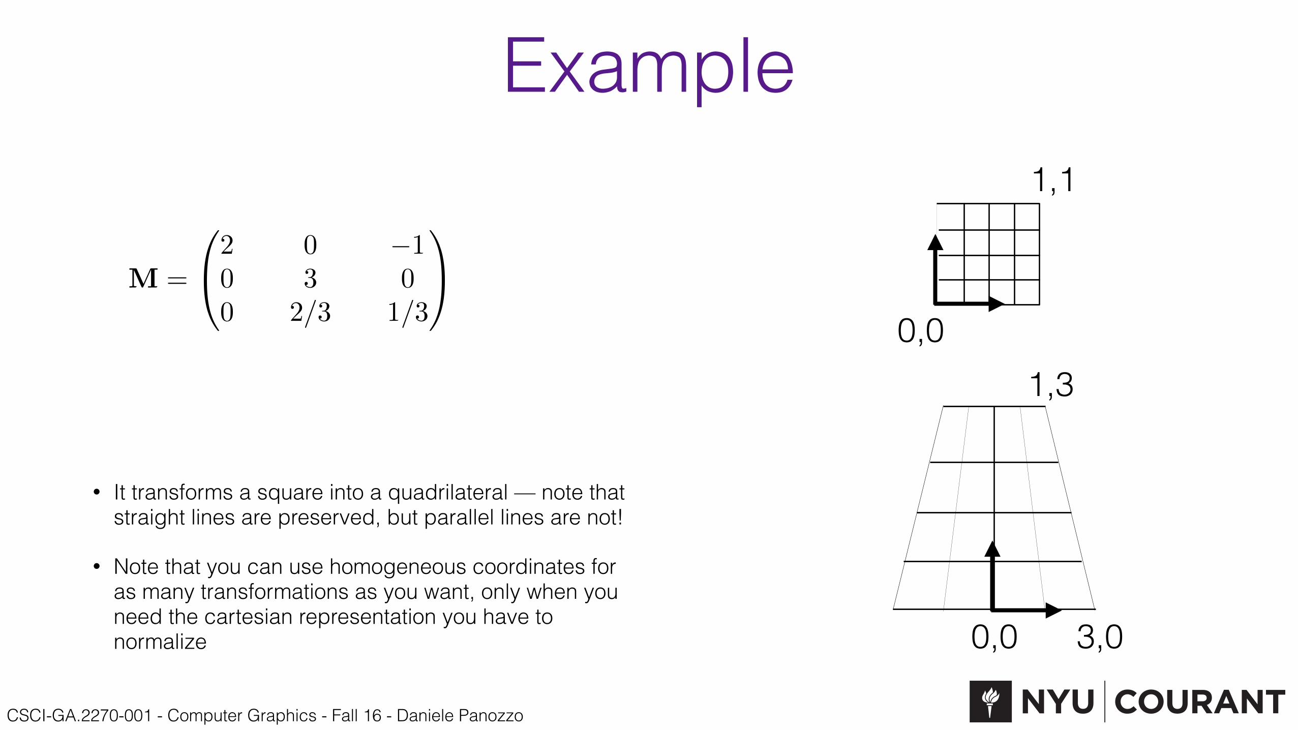
Example
• It transforms a square into a quadrilateral — note that straight lines are preserved, but parallel lines are not!
• Note that you can use homogeneous coordinates for as many transformations as you want, only when you need the cartesian representation you have to normalize
0,0
1,1
0,0 3,0
1,3
M =
0
@2 0 �10 3 00 2/3 1/3
1
A
CSCI-GA.2270-001 - Computer Graphics - Fall 16 - Daniele Panozzo
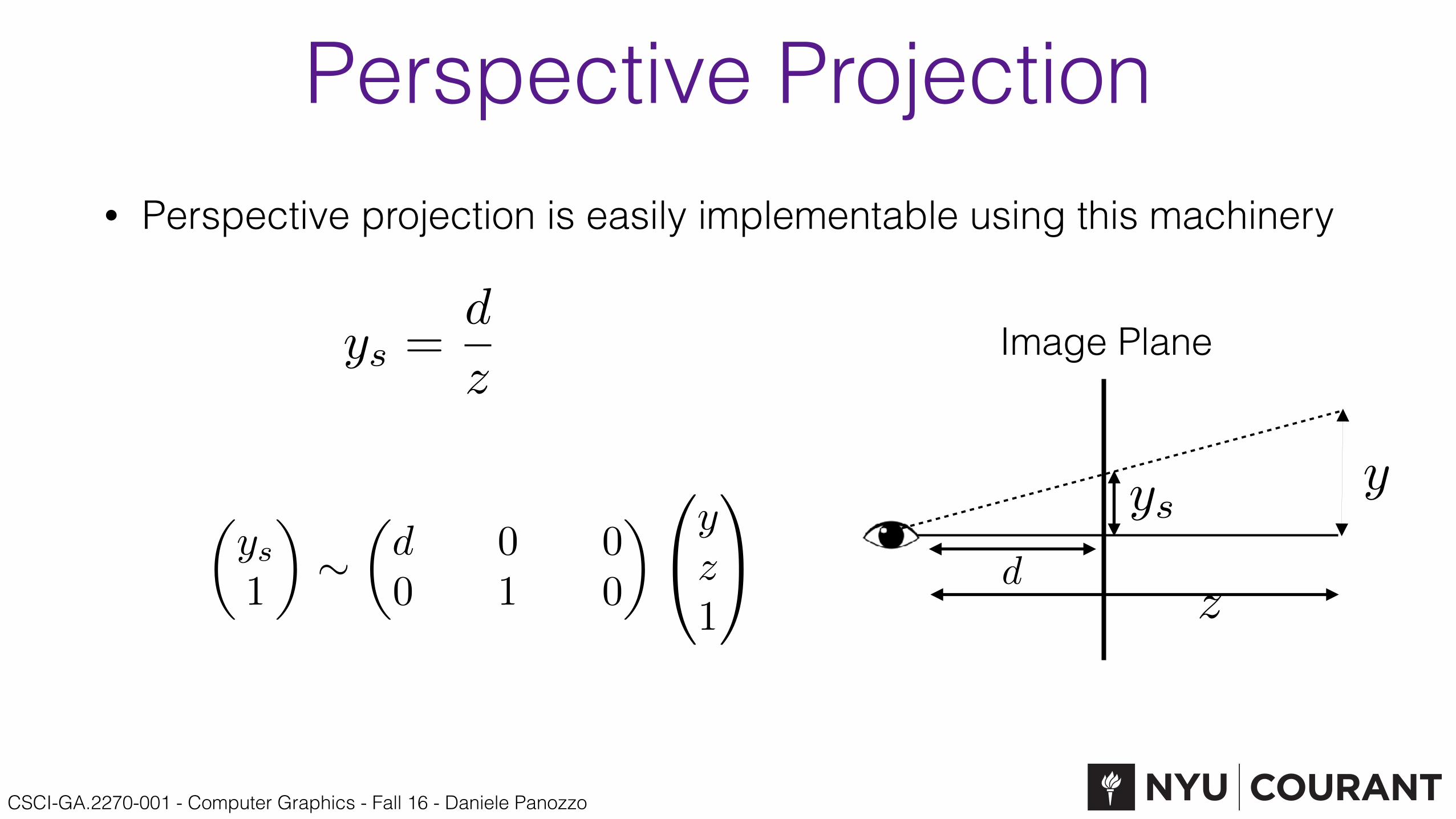
Perspective Projection• Perspective projection is easily implementable using this machinery
ysy
dz
ys =d
zImage Plane
✓ys1
◆⇠
✓d 0 00 1 0
◆0
@yz1
1
A
CSCI-GA.2270-001 - Computer Graphics - Fall 16 - Daniele Panozzo
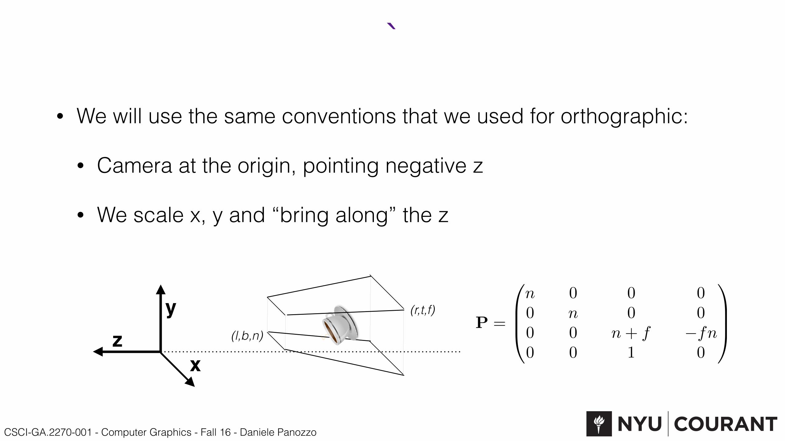
• We will use the same conventions that we used for orthographic:
• Camera at the origin, pointing negative z
• We scale x, y and “bring along” the z
`
xz
y(l,b,n)
(r,t,f)P =
0
BB@
n 0 0 00 n 0 00 0 n+ f �fn0 0 1 0
1
CCA
CSCI-GA.2270-001 - Computer Graphics - Fall 16 - Daniele Panozzo
Effect on the points
xz
y(l,b,n)
(r,t,f)P =
0
BB@
n 0 0 00 n 0 00 0 n+ f �fn0 0 1 0
1
CCA
P
0
BB@
x
y
z
1
1
CCA =
0
BB@
nx
ny
(n+ f)z � fn
z
1
CCA ⇠
0
BB@
nx
z
ny
z
n+ f � fn
z
1
1
CCA

CSCI-GA.2270-001 - Computer Graphics - Fall 16 - Daniele Panozzo
Effect on the points
xz
y(l,b,n)
(r,t,f)P =
0
BB@
n 0 0 00 n 0 00 0 n+ f �fn0 0 1 0
1
CCA
P
0
BB@
x
y
z
1
1
CCA =
0
BB@
nx
ny
(n+ f)z � fn
z
1
CCA ⇠
0
BB@
nx
z
ny
z
n+ f � fn
z
1
1
CCA

CSCI-GA.2270-001 - Computer Graphics - Fall 16 - Daniele Panozzo
Orthographic Projection
projection
canonical view volume
camera space
xz
y(l,b,n)
(r,t,f)
Morth
=
2
664
2r�l
0 0 � r+l
r�l
0 2t�b
0 � t+b
t�b
0 0 2n�f
�n+f
n�f
0 0 0 1
3
775
CSCI-GA.2270-001 - Computer Graphics - Fall 16 - Daniele Panozzo
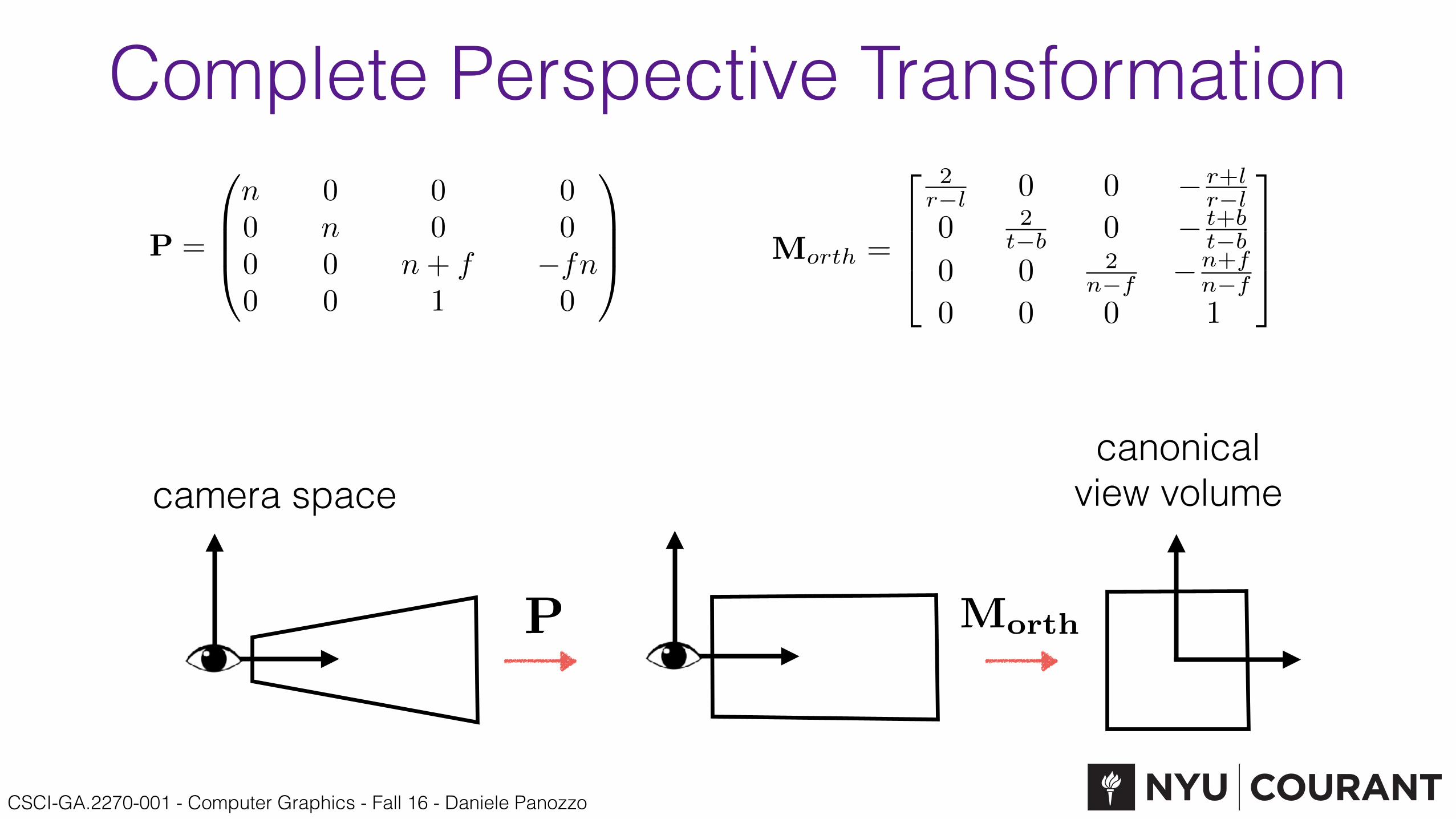
Complete Perspective Transformation
P =
0
BB@
n 0 0 00 n 0 00 0 n+ f �fn0 0 1 0
1
CCA
canonical view volumecamera space
P Morth
Morth
=
2
664
2r�l
0 0 � r+l
r�l
0 2t�b
0 � t+b
t�b
0 0 2n�f
�n+f
n�f
0 0 0 1
3
775
CSCI-GA.2270-001 - Computer Graphics - Fall 16 - Daniele Panozzo
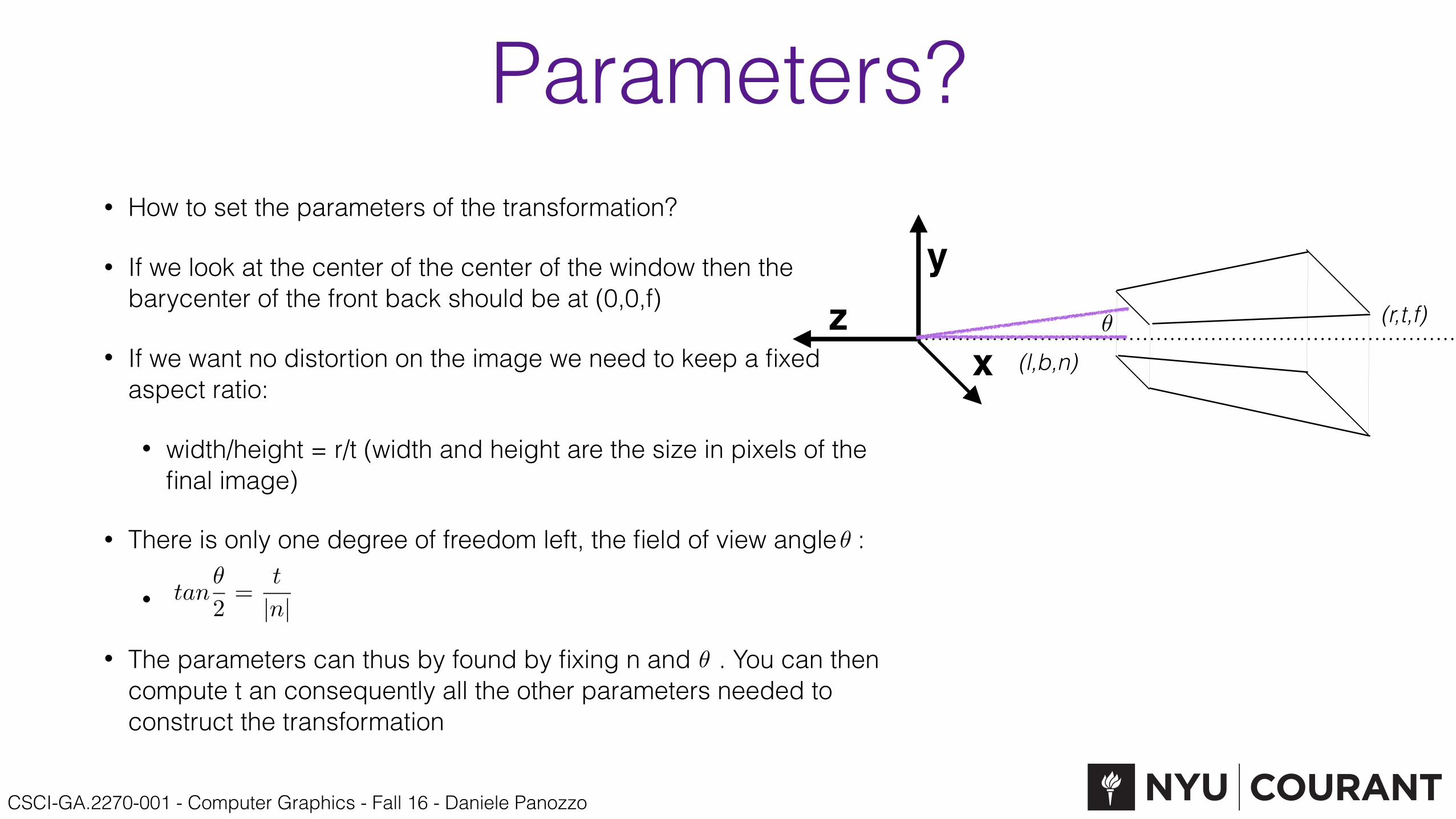
Parameters?• How to set the parameters of the transformation?
• If we look at the center of the center of the window then the barycenter of the front back should be at (0,0,f)
• If we want no distortion on the image we need to keep a fixed aspect ratio:
• width/height = r/t (width and height are the size in pixels of the final image)
• There is only one degree of freedom left, the field of view angle :
•
• The parameters can thus by found by fixing n and . You can then compute t an consequently all the other parameters needed to construct the transformation
xz
y
(l,b,n)
(r,t,f)
✓
tan✓
2=
t
|n|
✓
✓
CSCI-GA.2270-001 - Computer Graphics - Fall 16 - Daniele Panozzo
References
Fundamentals of Computer Graphics, Fourth Edition 4th Edition by Steve Marschner, Peter Shirley
Chapter 7