Neural Networks

Chapter 3

2

Outline

3.1 Introduction

3.2 Training Single TLUs

– Gradient Descent

– Widrow-Hoff Rule

– Generalized Delta Procedure

3.3 Neural Networks

– The Backpropagation Method

– Derivation of the Backpropagation Learning Rule

3.4 Generalization, Accuracy, and Overfitting

3.5 Discussion

3

3.1 Introduction

TLU (threshold logic unit): Basic units for neural networks

– Based on some properties of biological neurons

Training set

– Input: real value, boolean value, …

– Output:

: associated actions (Label, Class …)

Target of training

– Finding corresponds “acceptably” to the members of

the training set.

– Supervised learning: Labels are given along with the input

vectors.

jd

),...,(X vector,dim-n :X 1 nxx

( )f X

4

3.2.1 TLU Geometry

Training TLU: Adjusting variable weights

A single TLU: Perceptron, Adaline (adaptive linear element)

[Rosenblatt 1962, Widrow 1962]

Elements of TLU

– Weight:

– Threshold:

Output of TLU: Using weighted sum

– 1 if s > 0

– 0 if s < 0

Hyperplane

– WX = 0

1( ,..., )nW w w

s W X

5

6

3.2.2 Augmented Vectors

Adopting the convention that threshold is fixed to 0.

Arbitrary thresholds: (n + 1)-dimensional vector

W = (w1, …, wn, 1)

Output of TLU

– 1 if WX 0

– 0 if WX < 0

7

3.2.3 Gradient Decent Methods

Training TLU: minimizing the error function by adjusting weight values.

Two ways: Batch learning v.s. incremental learning

Commonly used error function: squared error

– Gradient :

– Chain rule:

Solution of nonlinearity of f / s :

– Ignoring threshod function: f = s

– Replacing threshold function with differentiable nonlinear

function

2)( fd

11

,...,,...,ni

def

www

W

XXWW s

ffd

s

s

s

)(2

8

3.2.4 The Widrow-Hoff Procedure

Weight update procedure:

– Using f = s = WX

– Data labeled 1 1, Data labeled 0 1

Gradient:

New weight vector

Widrow-Hoff (delta) rule

– (d f) > 0 increasing s decreasing (d f)

– (d f) < 0 decreasing s increasing (d f)

XXW

)(2)(2 fds

ffd

XWW )( fdc

9

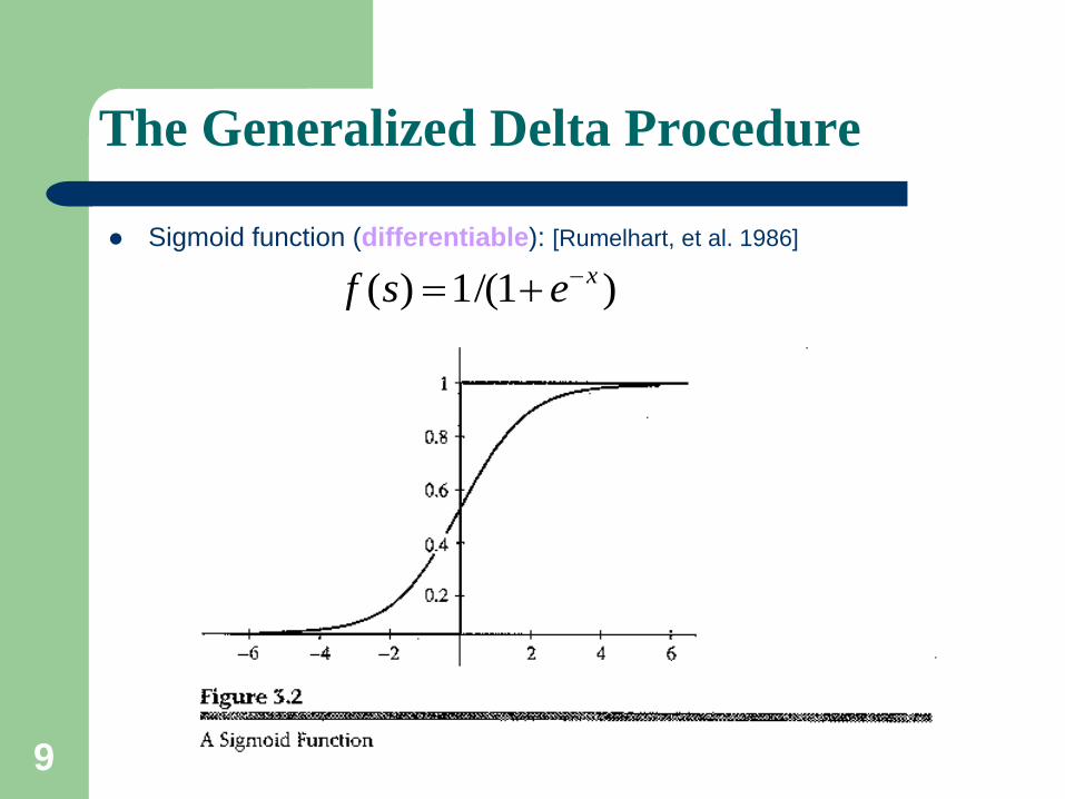
The Generalized Delta Procedure

Sigmoid function (differentiable): [Rumelhart, et al. 1986]

)1/(1)( xesf

10

The Generalized Delta Procedure (II)

Gradient:

Generalized delta procedure:

– Target output: 1, 0

– Output f = output of sigmoid function

– f(1– f) = 0, where f = 0 or 1

– Weight change can occur only within „fuzzy‟ region surrounding the hyperplane (near the point f(s) = ½).

XXW

)1()(2)(2 fffds

ffd

XWW )1()( fffdc

11

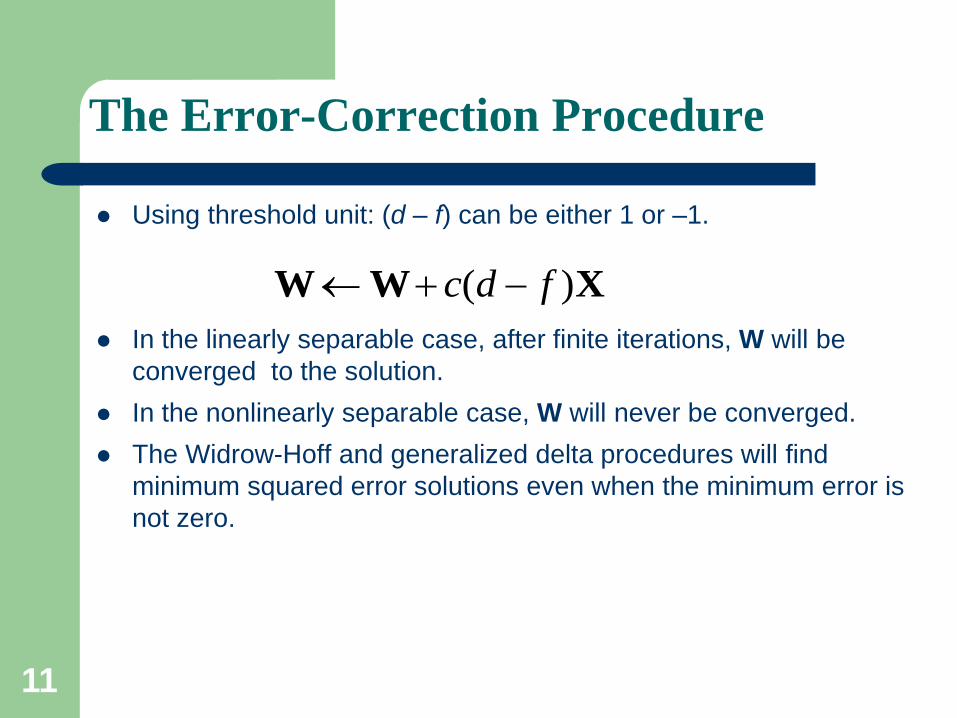
The Error-Correction Procedure

Using threshold unit: (d – f) can be either 1 or –1.

In the linearly separable case, after finite iterations, W will be

converged to the solution.

In the nonlinearly separable case, W will never be converged.

The Widrow-Hoff and generalized delta procedures will find

minimum squared error solutions even when the minimum error is

not zero.

XWW )( fdc

12

Training Process

Data L

kkdkX

1))(),((

)()(

)2()2(

)1()1(

LdLX

dX

dX

NN

X(k) f(k)

d(k)

-

)())()(()()( kkfkdckk XWW

• Update Rule

13

3.3 Neural Networks

Need for use of multiple TLUs

– Feedforward network: no cycle

– Recurrent network: cycle (treated in a later chapter)

– Layered feedforward network

jth layer can receive input only from j – 1th layer.

Example :

2121 xxxxf

14

Notation

Hidden unit: neurons in all but the last layer

Output of j-th layer: X(j) input of (j+1)-th layer

Input vector: X(0)

Final output: f

The weight of i-th sigmoid unit in the j-th layer: Wi(j)

Weighted sum of i-th sigmoid unit in the j-th layer: si(j)

Number of sigmoid units in j-th layer: mj

)()1()( j

i

jj

is WX

)(

,1

)(

,

)(

,1

)(

)1(,...,,..., j

im

j

il

j

i

j

i jwww

W

15

그림 3.5

16

3.3.3 The Backpropagation Method

Gradient of Wi(j) :

Weight update:

)()1()( j

i

jj

is WX

)()(

2

)()(2

)(j

i

j

i

j

i s

ffd

s

fd

s

)1()()()()( jj

i

j

i

j

i

j

i c XWW

)1()()1(

)(

)1(

)()(

)(

)()(

2)(2

jj

i

j

j

i

j

j

i

j

i

j

i

j

i

j

i

s

ffd

s

s

s

XX

XWW

Local gradient

17

Weight Changes in the Final Layer

Local gradient:

Weight update:

)1()(

)()(

)(

fffd

s

ffd

j

i

k

)1()()()( )1()( kkkk fffdc XWW

18

3.3.5 Weights in Intermediate Layers

Local gradient:

– The final ouput f, depends on si(j) through of the summed

inputs to the sigmoids in the (j+1)-th layer.

Need for computation of

)(

)1(

1

)1(

)(

)1(

)1(1

)(

)1(

)1()(

)1(

)1()(

)1(

1

)1(

1

)(

)(

11

1

1

)(

......)(

)(

j

i

j

l

m

l

j

lj

i

j

l

j

l

m

l

j

i

j

m

j

m

j

i

j

l

j

l

j

i

j

j

j

i

j

i

s

s

s

s

s

ffd

s

s

s

f

s

s

s

f

s

s

s

ffd

s

ffd

jj

j

j

)(

)1(

j

i

j

l

s

s

19

Weight Update in Hidden Layers (cont.)

– v i : v = i :

– Conseqeuntly,

)1( )()()1(

,

1

1)(

)()1(

,)(

1

1

)1(

,

)(

)(

)1(

1

1

)1(

,

)()1()()1(

j

i

j

i

j

li

m

vj

i

j

vj

lvj

i

m

v

j

lv

l

v

j

i

j

l

m

v

j

lv

l

v

j

l

jj

l

ffw

s

fw

s

wf

s

s

wfs

jj

j

WX

0)(

)(

j

i

j

v

s

f)1( )()(

)(

)(j

v

j

vj

i

j

v ffs

f

1

1

)1(

.

)1()()()( )1(jm

l

j

li

j

l

j

i

j

i

j

i wff

20

Weight Update in Hidden Layers (cont.)

Attention to recursive equation of local gradient!

Backpropagation:

– Error is back-propagated from the output layer to the input layer

– Local gradient of the latter layer is used in calculating local

gradient of the former layer.

))(1()( fdffk

1

1

)1(

.

)1()()()( )1(jm

l

j

li

j

i

j

i

j

i

j

i wff

21

3.3.5 (con’t)

Example (even parity function)

– Learning rate: 1.0

input target

1 0 1 0

0 0 1 1

0 1 1 0

1 1 1 1

2121 xxxxf

22

Generalization, Accuracy, Overfitting

Generalization ability:

– NN appropriately classifies vectors not in the training set.

– Measurement = accuracy

Curve fitting

– Number of training input vectors number of degrees of freedom of the network.

– In the case of m data points, is (m-1)-degree polynomial best model? No, it can not capture any special information.

Overfitting

– Extra degrees of freedom are essentially just fitting the noise.

– Given sufficient data, the Occam’s Razor principle dictates to choose the lowest-degree polynomial that adequately fits the data.

23

Overfitting

24

Generalization (cont’d)

Out-of-sample-set error rate

– Error rate on data drawn from the same underlying distribution of

training set.

Dividing available data into a training set and a validation set

– Usually use 2/3 for training and 1/3 for validation

k-fold cross validation

– k disjoint subsets (called folds).

– Repeat training k times with the configuration: one validation set,

k-1 (combined) training sets.

– Take average of the error rate of each validation as the out-of-

sample error.

– Empirically 10-fold is preferred.

25

Fig 3.8 Error Versus Number of

Hidden Units

Fig 9. Estimate of Generalization Error

Versus Number of Hidden Units

26

3.5 Additional Readings & Discussion

Applications

– Pattern recognition, automatic control, brain-function modeling

– Designing and training neural networks still need experience and

experiments.

Major annual conferences

– Neural Information Processing Systems (NIPS)

– International Conference on Machine Learning (ICML)

– Computational Learning Theory (COLT)

Major journals

– Neural Computation

– IEEE Transactions on Neural Networks

– Machine Learning

27

Homework

Page 55 ~ 57

– Ex 3.1; Ex3.4, Ex3.6, Ex. 3.7

How to submit your homework:

Email to lqzhang@sjtu.edu.cn

Filename specification: [学号]+[姓名]+[章节].doc