Statistical & Data Analysis Using Neural Network · · 2015-03-12Statistical & Data Analysis...

Statistics & Data Analysis using Neural Network

Copyrighted 2005 TechSource Systems Sdn Bhd 1

www.techsource.com.my

©2005 Systems Sdn. Bhd.

Statistical & Data Analysis Using Neural Network

TechSource Systems Sdn. Bhd.



Course Outline:1. Neural Network Concepts

a) Introductionb) Simple neuron modelc) MATLAB representation of neural network

2. Types of Neural Networka) Perceptronsb) Linear networksc) Backpropagation networksd) Self-organizing maps

3. Case Study: Predicting Time Series





Neural Network Concepts

Section Outline:1. Introduction

Definition of neural networkBiological perspective of neural networkNeural network applications

2. Simple neuron modelComponents of simple neuron

3. MATLAB representation of neural networkSingle neuron modelNeural network with single-layer of neuronsNeural network with multiple-layer of neurons




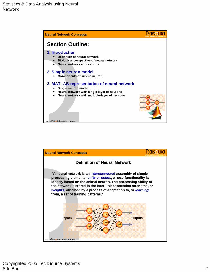
Definition of Neural Network

“A neural network is an interconnected assembly of simple processing elements, units or nodes, whose functionality is loosely based on the animal neuron. The processing ability of the network is stored in the inter-unit connection strengths, or weights, obtained by a process of adaptation to, or learningfrom, a set of training patterns.”

Inputs Outputs





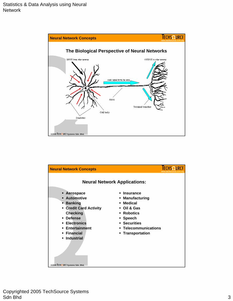
The Biological Perspective of Neural Networks




Neural Network Applications:

AerospaceAutomotiveBankingCredit Card Activity CheckingDefenseElectronicsEntertainmentFinancialIndustrial

InsuranceManufacturingMedicalOil & GasRoboticsSpeechSecuritiesTelecommunicationsTransportation







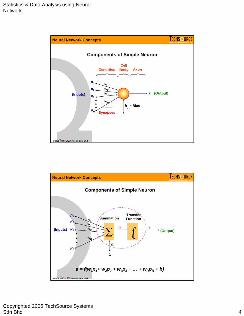
Components of Simple Neuron

•••

p1

p2

p3

pR

w1w2w3

wR

a

DendritesCell

Body Axon

Synapses

(Inputs) (Output)

1

b Bias



Components of Simple Neuron

a = f(w1p1+ w2p2 + w3p3 + … + wRpR + b)

Σ ƒ•••

SummationTransfer Functionw1

w2w3

wR

b

1

p1

p2

p3

pR

a(Inputs) (Output)n







Σ n aInputs Output

p1

p2

w1

w2

1

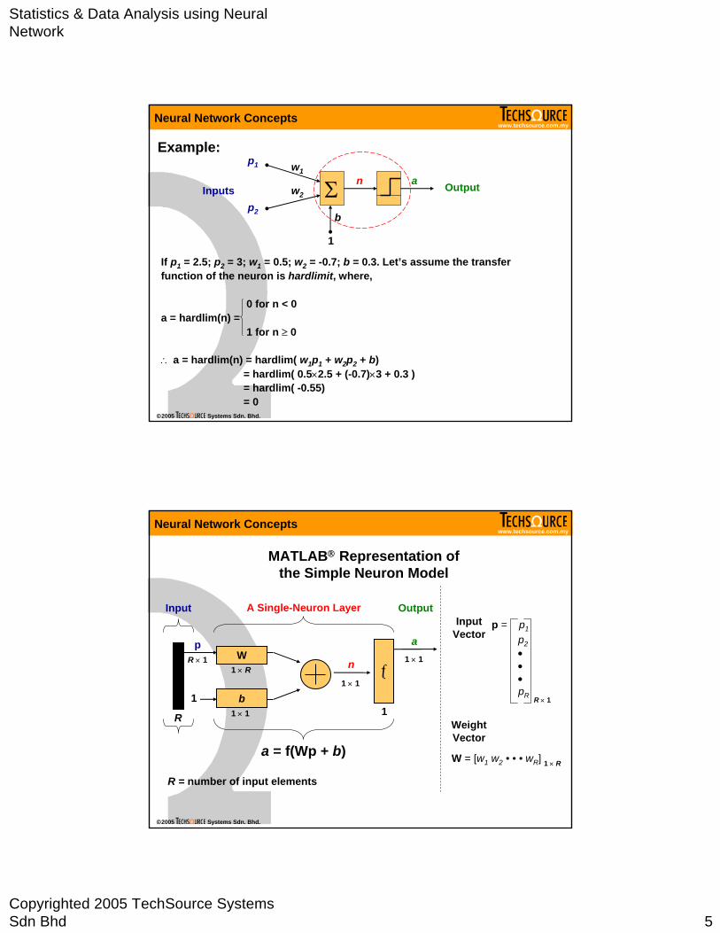
If p1 = 2.5; p2 = 3; w1 = 0.5; w2 = -0.7; b = 0.3. Let’s assume the transfer function of the neuron is hardlimit, where,

0 for n < 0a = hardlim(n) =

1 for n ≥ 0

∴ a = hardlim(n) = hardlim( w1p1 + w2p2 + b)= hardlim( 0.5×2.5 + (-0.7)×3 + 0.3 )= hardlim( -0.55)= 0

b

Example:




MATLAB® Representation of the Simple Neuron Model

W

b

ƒ

R

Input A Single-Neuron Layer Output

R × 1

p

1

1 × R

1 × 1

n1 × 1

1

a1 × 1

a = f(Wp + b)

p = p1

p2•••pR R × 1

Input Vector

Weight Vector

W = [w1 w2 • • • wR] 1 × R

R = number of input elements






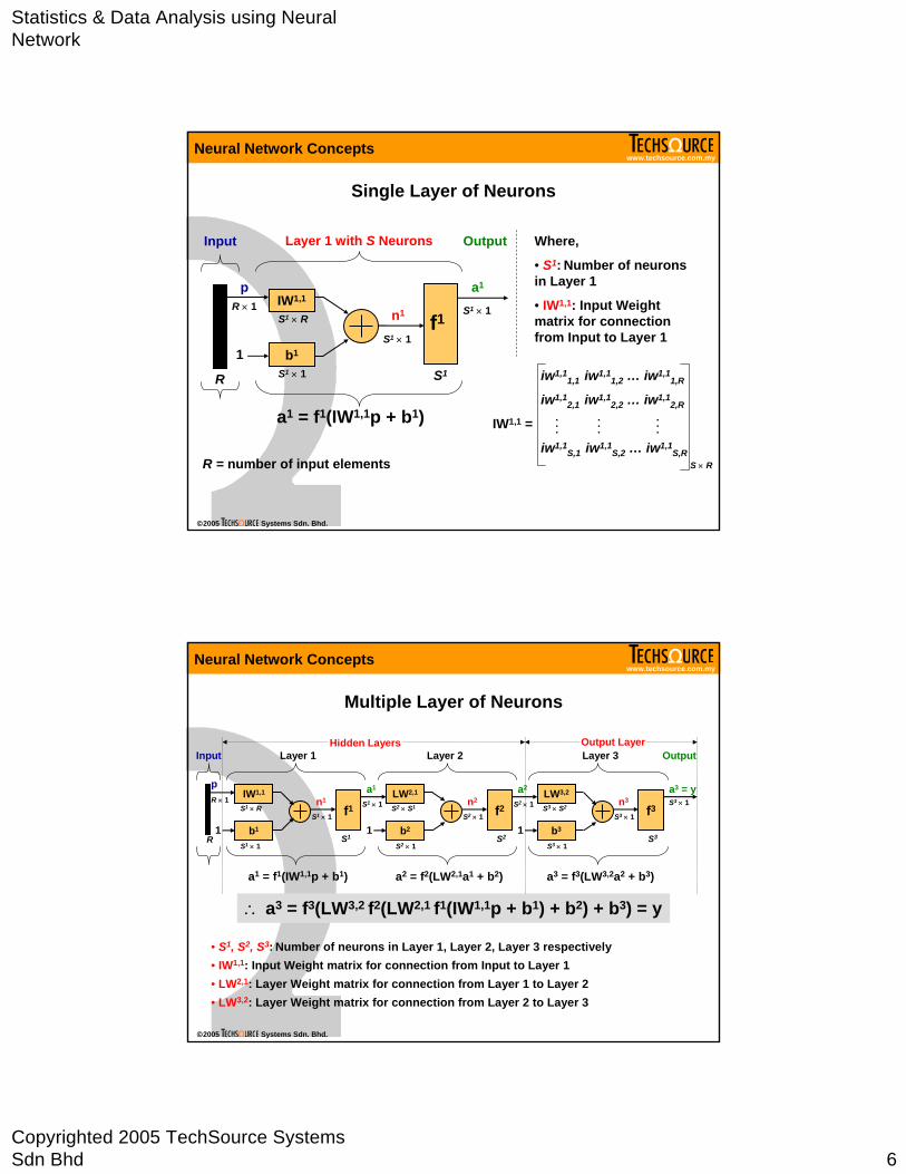
Single Layer of Neurons

IW1,1

b1

f1

R

Input Layer 1 with S Neurons Output

R × 1

p

1

S1 × R

S1 × 1

n1

S1 × 1

S1

a1

S1 × 1

a1 = f1(IW1,1p + b1)

R = number of input elements

Where,

• S1: Number of neurons in Layer 1

• IW1,1: Input Weight matrix for connection from Input to Layer 1

iw1,11,1 iw1,1

1,2 … iw1,11,R

iw1,12,1 iw1,1

2,2 … iw1,12,R

IW1,1 =

iw1,1S,1 iw1,1

S,2 … iw1,1S,R

......

...

S × R




IW1,1

b1

f1R × 1

p

1

n1

S1

LW2,1

b2

f2LW3,2

b3

f3

1 1

Input Layer 1 Layer 2 Layer 3

S1 × R

S1 × 1

a1

S1 × 1S1 × 1

S2 × 1S2

n2

S2 × 1S2 × S1

a2

S2 × 1 S3 × S2

S3 × 1

n3

S3 × 1

S3

a3 = y

Output

S3 × 1

a1 = f1(IW1,1p + b1) a2 = f2(LW2,1a1 + b2) a3 = f3(LW3,2a2 + b3)

∴ a3 = f3(LW3,2 f2(LW2,1 f1(IW1,1p + b1) + b2) + b3) = y

• S1, S2, S3: Number of neurons in Layer 1, Layer 2, Layer 3 respectively• IW1,1: Input Weight matrix for connection from Input to Layer 1• LW2,1: Layer Weight matrix for connection from Layer 1 to Layer 2• LW3,2: Layer Weight matrix for connection from Layer 2 to Layer 3

Hidden Layers Output Layer

R

Multiple Layer of Neurons






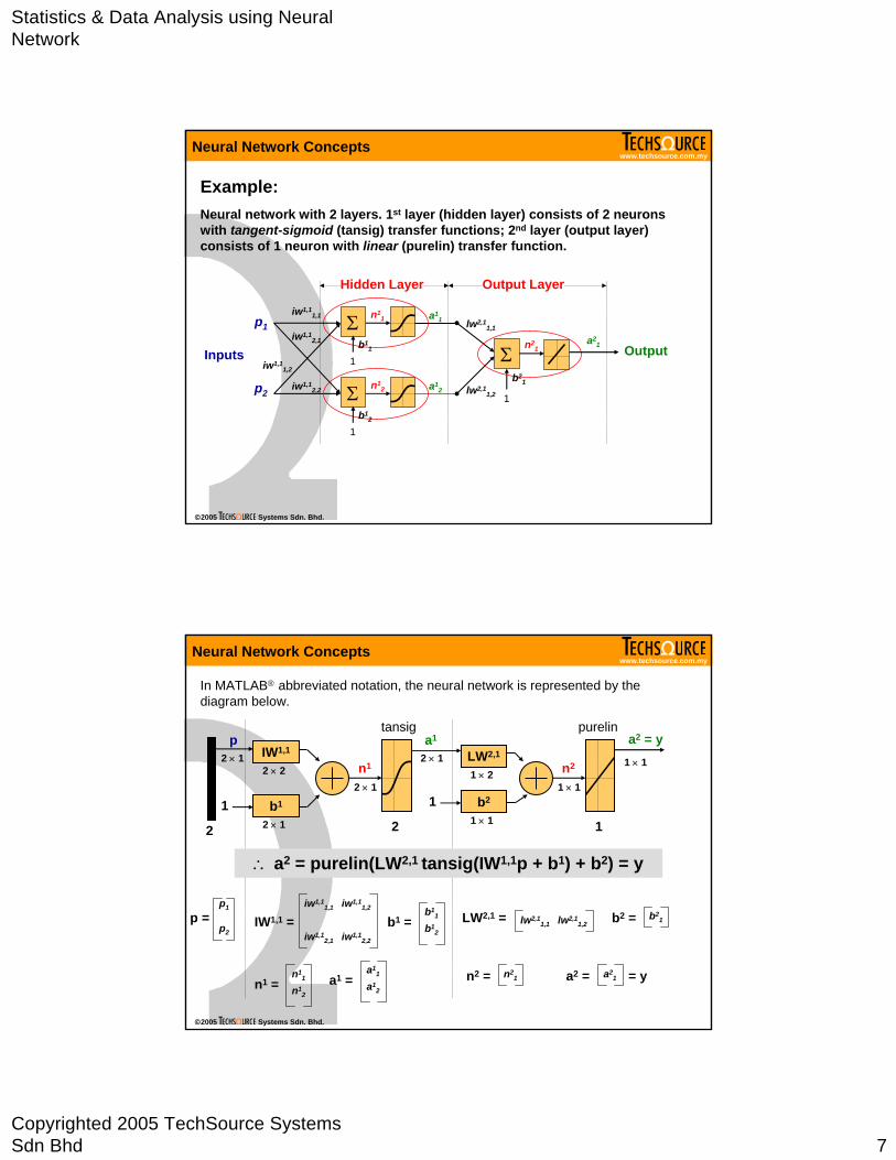
Example:

Σ

Σ

Σ

p1

p2

1

n11

n12

n21

a11

a12

a21

1

b11

b12

b21

iw1,11,1

iw1,11,2

iw1,12,1

iw1,12,2

lw2,11,1

lw2,11,2

1

Inputs

Hidden Layer Output Layer

Neural network with 2 layers. 1st layer (hidden layer) consists of 2 neurons with tangent-sigmoid (tansig) transfer functions; 2nd layer (output layer) consists of 1 neuron with linear (purelin) transfer function.

Output




In MATLAB® abbreviated notation, the neural network is represented by the diagram below.

IW1,1

b1

2

2 × 1p

1

2 × 2

2 × 1

n1

2 × 1

2

a1

2 × 1 LW2,1

b2

n2

1 × 1

1

a2 = y1 × 1

1 × 2

11 × 1

IW1,1 = iw1,1

1,1 iw1,11,2

iw1,12,1 iw1,1

2,2

p =p1

p2b1 =

b11

b12

n1 =n1

1

n12

a1 =a1

1

a12

LW2,1 = lw2,11,1 lw2,1

1,2 b2 = b21

n2 = n21 a2 = a2

1 = y

∴ a2 = purelin(LW2,1 tansig(IW1,1p + b1) + b2) = y

tansig purelin






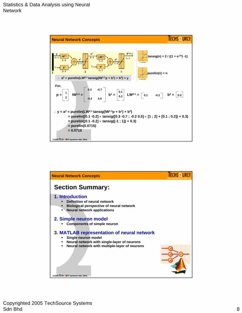
tansig(n) = 2 / ((1 + e-2n) -1)

purelin(n) = n

IW1,1 = 0.3 -0.7

-0.2 0.5p = 1

2b1 =

0.10.2 LW2,1 = 0.1 -0.2 b2 = 0.3


For,

∴y = a2 = purelin(LW2,1 tansig(IW1,1p + b1) + b2)= purelin([0.1 -0.2] × tansig([0.3 -0.7 ; -0.2 0.5] × [1 ; 2] + [0.1 ; 0.2]) + 0.3)= purelin([0.1 -0.2] × tansig([-1 ; 1]) + 0.3)= purelin(0.0715)= 0.0715




Section Summary:1. Introduction

Definition of neural networkBiological perspective of neural networkNeural network applications

2. Simple neuron modelComponents of simple neuron

3. MATLAB representation of neural networkSingle neuron modelNeural network with single-layer of neuronsNeural network with multiple-layer of neurons





Types of Neural Network

Section Outline:1. Perceptrons

IntroductionThe perceptron architectureTraining of perceptronsApplication examples

2. Linear NetworksIntroductionArchitecture of linear networksThe Widrow-Hoff learning algorithmApplication examples

3. Backpropagation NetworksIntroductionArchitecture of backprogation networkThe backpropagation algorithmTraining algorithmsPre- and post-processingApplication examples

4. Self-Organizing MapsIntroductionCompetitive learningSelf-organizing mapsApplication examples



Perceptrons

Invented in 1957 by Frank Rosenblatt at Cornell Aeronautical Laboratory.

The perceptron consists of a single-layer of neurons whose weights and biases could be trained to produce a correct target vector when presented with corresponding input vector.

The output from a single perceptron neuron can only be in one of the two states. If the weighted sum of its inputs exceeds a certain threshold, the neuron will fire by outputting 1; otherwise the neuron will output either 0 or -1, depending on the transfer function used.

The perceptron can only solve linearly separable problems.






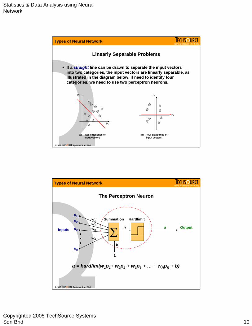
If a straight line can be drawn to separate the input vectors into two categories, the input vectors are linearly separable, as illustrated in the diagram below. If need to identify four categories, we need to use two perceptron neurons.

Linearly Separable Problems

p1

p2

(a) Two categories of input vectors

(b) Four categories of input vectors

p1

p2




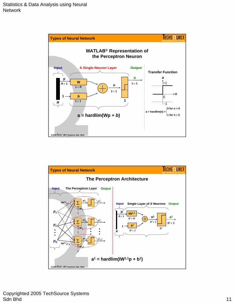
The Perceptron Neuron

Σ•••

Summation Hardlimitw1w2w3

wR

b

1

p1

p2

p3

pR

a

a = hardlim(w1p1+ w2p2 + w3p3 + … + wRpR + b)

Inputs Outputn






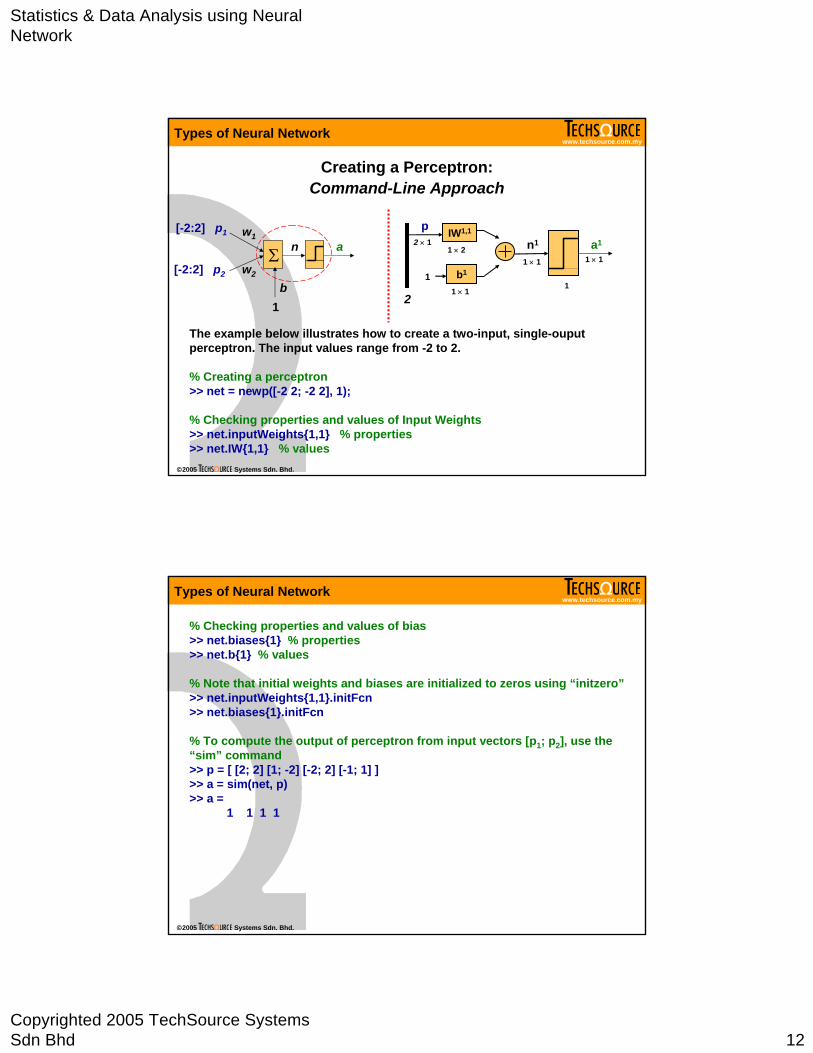
MATLAB® Representation of the Perceptron Neuron

W

b

R


R × 1

p

1

1 × R

1 × 1

n1 × 1

1

a1 × 1

a = hardlim(Wp + b)

a

0

+1

n

-1

Transfer Function

0 for n < 0a = hardlim(n) =

1 for n ≥ 0




The Perceptron Architecture

Σ

Σ

p1

p2

1

n11

n12

a11

a12

b11

b12

iw1,11,1

1

Σ n1S1 a1

S1

b1S1

1

iw1,1S1,R

•••

pR

•••

•••

Input The Perceptron Layer Output

IW1,1

b1

R

Single Layer of S Neurons Output

R × 1

p

1

S1 × R

S1 × 1

n1

S1 × 1

S1

a1

S1 × 1

a1 = hardlim(IW1,1p + b1)

Input






Creating a Perceptron: Command-Line Approach

The example below illustrates how to create a two-input, single-ouput perceptron. The input values range from -2 to 2.

% Creating a perceptron>> net = newp([-2 2; -2 2], 1);

% Checking properties and values of Input Weights>> net.inputWeights{1,1} % properties>> net.IW{1,1} % values

Σ

[-2:2] p1

[-2:2] p2

w1

w2

n

b1

aIW1,1

b1

2

2 × 1

p

1

1 × 2

1 × 1

n1

1 × 1

1

a1

1 × 1





% Checking properties and values of bias>> net.biases{1} % properties>> net.b{1} % values

% Note that initial weights and biases are initialized to zeros using “initzero”>> net.inputWeights{1,1}.initFcn>> net.biases{1}.initFcn

% To compute the output of perceptron from input vectors [p1; p2], use the “sim” command>> p = [ [2; 2] [1; -2] [-2; 2] [-1; 1] ] >> a = sim(net, p)>> a =

1 1 1 1





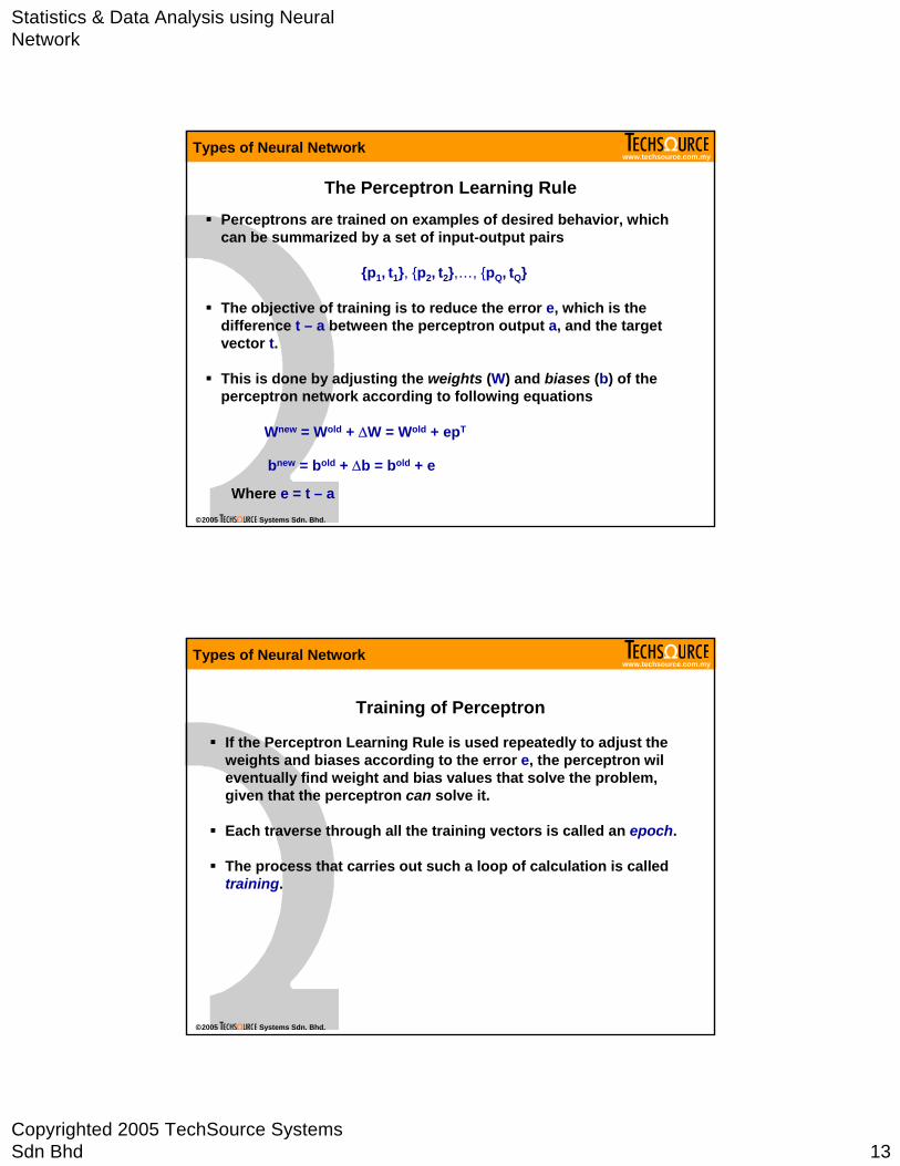
The Perceptron Learning Rule

Perceptrons are trained on examples of desired behavior, which can be summarized by a set of input-output pairs

{p1, t1}, {p2, t2},…, {pQ, tQ}

The objective of training is to reduce the error e, which is the difference t – a between the perceptron output a, and the target vector t.

This is done by adjusting the weights (W) and biases (b) of the perceptron network according to following equations

Wnew = Wold + ∆W = Wold + epT

bnew = bold + ∆b = bold + e

Where e = t – a




Training of Perceptron

If the Perceptron Learning Rule is used repeatedly to adjust theweights and biases according to the error e, the perceptron wil eventually find weight and bias values that solve the problem, given that the perceptron can solve it.

Each traverse through all the training vectors is called an epoch.

The process that carries out such a loop of calculation is called training.






10

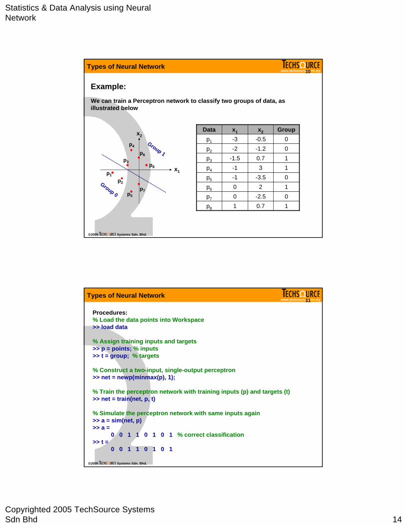
We can train a Perceptron network to classify two groups of data, as illustrated below

x1

x2

p1p2

p3

p4

p5

p6

p7

p8

Group 0

Group 1

0.7-2.5

2-3.5

30.7-1.2-0.5x2

11p8

00p7

10p6

0-1p5

1-1p4

1-1.5p3

0-2p2

0-3p1

Groupx1Data

Example:




11

Procedures:% Load the data points into Workspace>> load data

% Assign training inputs and targets>> p = points; % inputs>> t = group; % targets

% Construct a two-input, single-output perceptron>> net = newp(minmax(p), 1);

% Train the perceptron network with training inputs (p) and targets (t)>> net = train(net, p, t)

% Simulate the perceptron network with same inputs again>> a = sim(net, p)>> a =

0 0 1 1 0 1 0 1 % correct classification>> t =

0 0 1 1 0 1 0 1






12

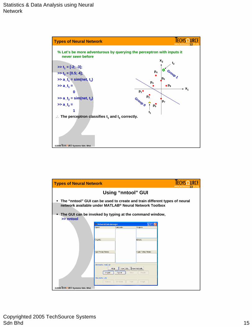
% Let’s be more adventurous by querying the perceptron with inputs it never seen before

>> t1 = [-2; -3];>> t2 = [0.5; 4];>> a_t1 = sim(net, t1)>> a_t1 =

0>> a_t2 = sim(net, t2)>> a_t2 =

1

x1

x2

p1

p2

p3

p4

p5

p6

p7

p8

Group 0

Group 1

t1

t2

∴ The perceptron classifies t1 and t2 correctly.




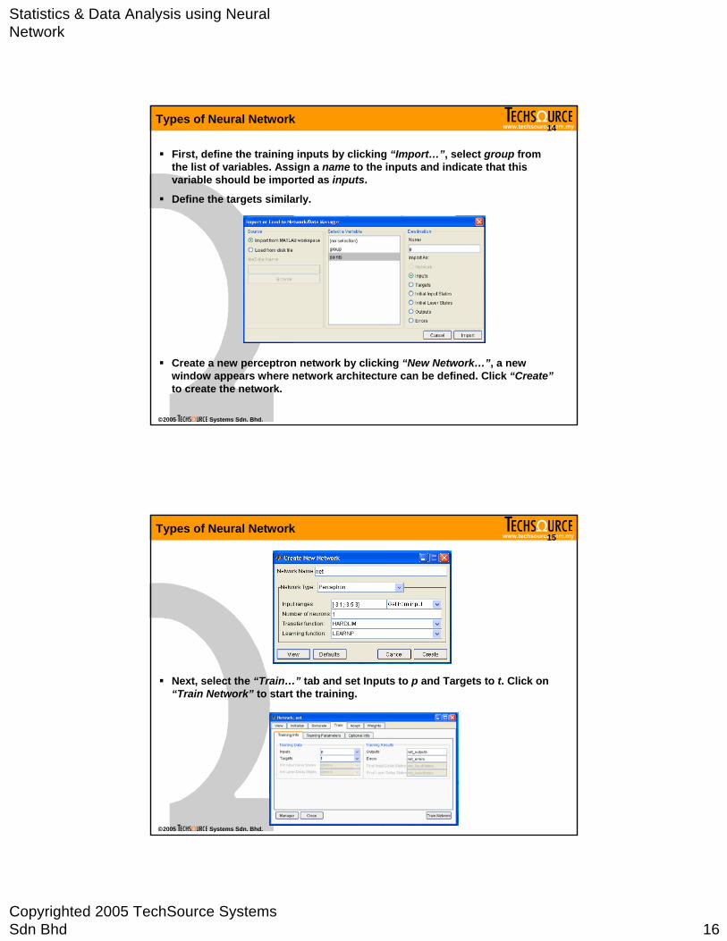
Using “nntool” GUIThe “nntool” GUI can be used to create and train different types of neural network available under MATLAB® Neural Network Toolbox

The GUI can be invoked by typing at the command window,>> nntool

13Types of Neural Network





14

Create a new perceptron network by clicking “New Network…”, a new window appears where network architecture can be defined. Click “Create”to create the network.

First, define the training inputs by clicking “Import…”, select group from the list of variables. Assign a name to the inputs and indicate that this variable should be imported as inputs.

Define the targets similarly.




15

Next, select the “Train…” tab and set Inputs to p and Targets to t. Click on “Train Network” to start the training.






The network completed training in 4 epochs, which is 4 complete passes through all training inputs.

Now, we can test the performance of the trained network by clicking “Simulate...”. Set the Inputs to p.




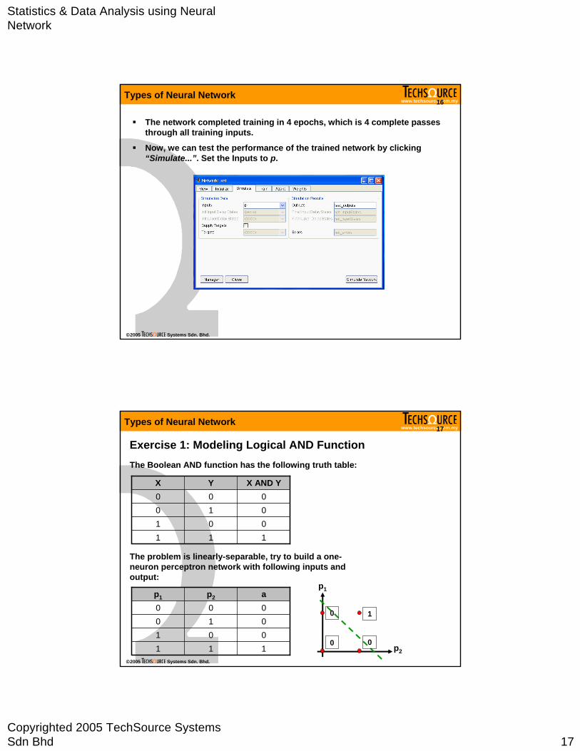
Exercise 1: Modeling Logical AND FunctionThe Boolean AND function has the following truth table:

111001010000

X AND YYX

The problem is linearly-separable, try to build a one-neuron perceptron network with following inputs and output:

111001010000ap2p1

1

p1

00

0

17

p2






18

Solution:Command-line approach is demonstrated herein. The “nntool” GUI can be used alternatively.

% Define at the MATLAB® command window, the training inputs and targets>> p = [0 0 1 1; 0 1 0 1]; % training inputs, p = [p1; p2]>> t = [0 0 0 1]; % targets

% Create the perceptron>> net = newp([0 1; 0 1], 1);

% Train the perceptron with p and t>> net = train(net, p, t);

% To test the performance, simulate the perceptron with p>> a = sim(net, p)>> a =

0 0 0 1>> t =

0 0 0 1




19

Exercise 2: Pattern Classification Build a perceptron that can differentiate between two group of images:

Hint:

Use Boolean values 1’s and 0’s to represent the image.

Example for image_1 is shown.

∴ image_1 = [ 0 1 01 0 11 0 10 1 0]’;

Load the training vectors into workspace:

>> load train_images

Group 0 Group 1

img2

0

img1

1 01 0 11 0 10 1 0

img3 img4






Try testing the trained perceptron on following images:

timg1 timg2 timg3

>> load test_images




Solution:Command-line approach is demonstrated herein. Tne “nntool” GUI can be used alternatively.

% Define at the MATLAB® command window, the training inputs and targets>> load train_images>> p = [img1 img2 img3 img4];>> t = targets;

% Create the perceptron>> net = newp(minmax(p), 1);

% Training the perceptron>> net = train(net, p, t);

% Testing the performance of the trained perceptron>> a = sim(net, p)

% Load the test images and ask the perceptron to classify it>> load test_images>> test1 = sim(net, timg1) % to do similarly for other test images






Linear Networks

Linear networks are similar to perceptron, but their transfer function is linear rather than hard-limiting.

Therefore, the output of a linear neuron is not limited to 0 or 1.

Similar to perceptron, linear network can only solve linearly separable problems.

Common applications of linear networks are linear classification and adaptive filtering.




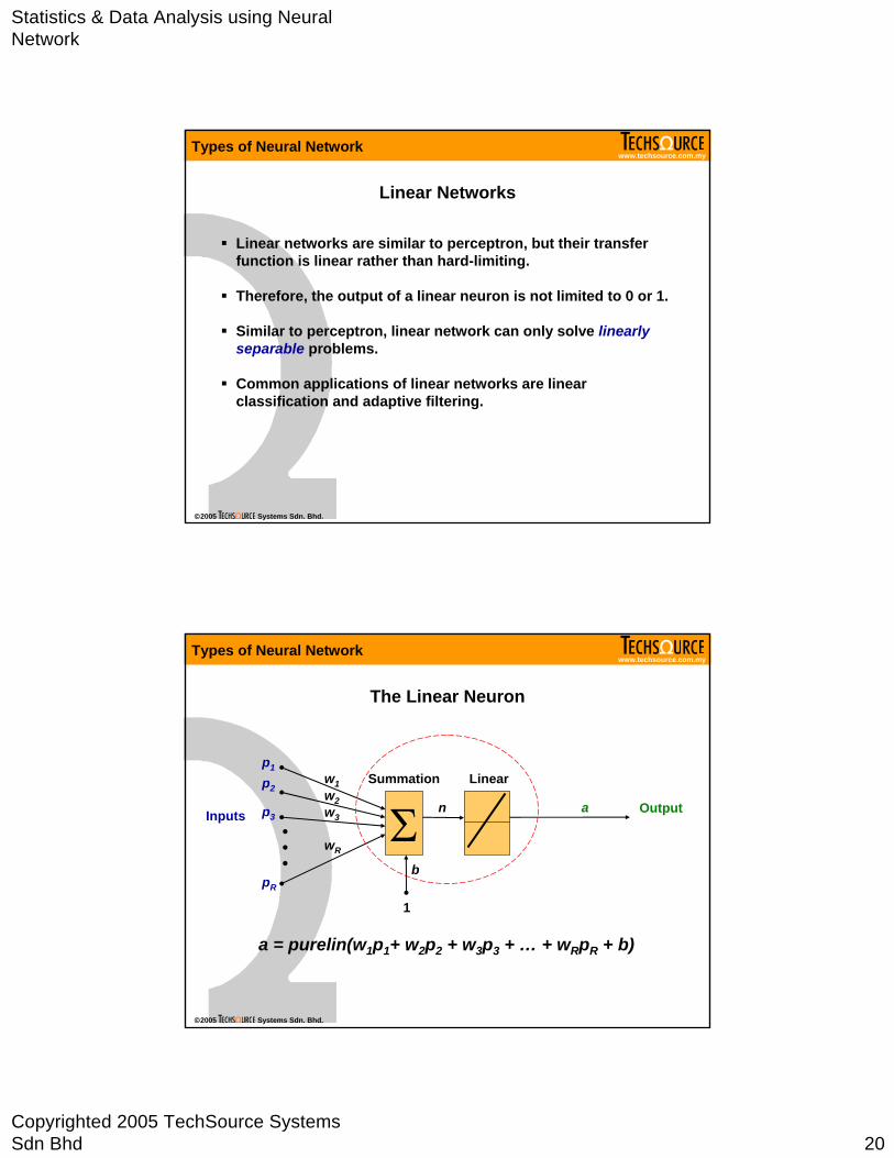
The Linear Neuron

Σ•••

Summation Linearw1w2w3

wR

b

1

p1

p2

p3

pR

a

a = purelin(w1p1+ w2p2 + w3p3 + … + wRpR + b)

Inputs Outputn






MATLAB® Representation of the Linear Neuron

a

0

+1

n

-1

Transfer Function

a = purelin(n) = n

W

b

R


R × 1

p

1

1 × R

1 × 1

n1 × 1

1

a1 × 1

a = purelin(Wp + b)




Architecture of Linear Networks

IW1,1

b1

R

Output

R × 1

p

1

S1 × R

S1 × 1

n1

S1 × 1

S1

a1

S1 × 1

a1 = purelin(IW1,1p + b1)

Input Layer of S1 Linear NeuronsΣ

Σ

p1

p2

1

n11

n12

a11

a12

b11

b12

iw1,11,1

1

Σ n1S1 a1

S1

b1S1

1

iw1,1S1,R

•••

pR

•••

•••

Input Layer of Linear Neurons Output






5

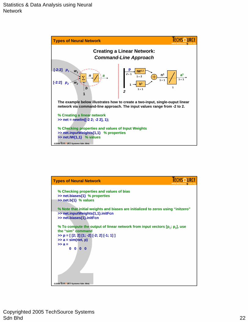
Creating a Linear Network: Command-Line Approach

The example below illustrates how to create a two-input, single-ouput linear network via command-line approach. The input values range from -2 to 2.

% Creating a linear network>> net = newlin([-2 2; -2 2], 1);

% Checking properties and values of Input Weights>> net.inputWeights{1,1} % properties>> net.IW{1,1} % values

Σ

[-2:2] p1

[-2:2] p2

w1

w2

n

b1

aIW1,1

b1

2

2 × 1

p

1

1 × 2

1 × 1

n1

1 × 1

1

a1

1 × 1




6

% Checking properties and values of bias>> net.biases{1} % properties>> net.b{1} % values

% Note that initial weights and biases are initialized to zeros using “initzero”>> net.inputWeights{1,1}.initFcn>> net.biases{1}.initFcn

% To compute the output of linear network from input vectors [p1; p2], use the “sim” command>> p = [ [2; 2] [1; -2] [-2; 2] [-1; 1] ] >> a = sim(net, p)>> a =

0 0 0 0






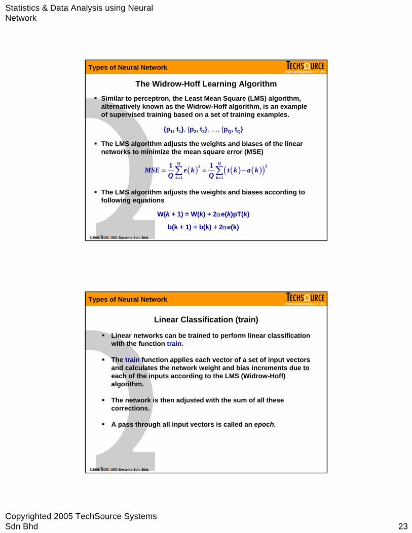
The Widrow-Hoff Learning Algorithm

Similar to perceptron, the Least Mean Square (LMS) algorithm, alternatively known as the Widrow-Hoff algorithm, is an example of supervised training based on a set of training examples.

{p1, t1}, {p2, t2}, …, {pQ, tQ}

The LMS algorithm adjusts the weights and biases of the linear networks to minimize the mean square error (MSE)

The LMS algorithm adjusts the weights and biases according to following equations

W(k + 1) = W(k) + 2αe(k)pT(k)

b(k + 1) = b(k) + 2αe(k)

( ) ( ) ( )( )22

1 1

1 1Q Q

k kMSE e k t k a k

Q Q= =

= = −∑ ∑




Linear Classification (train)

Linear networks can be trained to perform linear classification with the function train.

The train function applies each vector of a set of input vectors and calculates the network weight and bias increments due to each of the inputs according to the LMS (Widrow-Hoff) algorithm.

The network is then adjusted with the sum of all these corrections.

A pass through all input vectors is called an epoch.






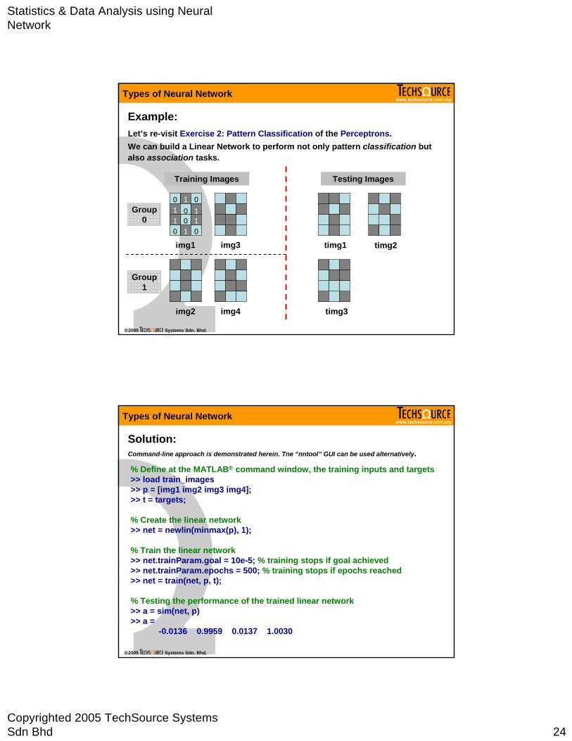
Example:Let’s re-visit Exercise 2: Pattern Classification of the Perceptrons. We can build a Linear Network to perform not only pattern classification but also association tasks.

Group 0

Group 1

img2

0

img1

1 01 0 11 0 10 1 0

img3

img4

Training Images Testing Images

timg1 timg2

timg3





% Define at the MATLAB® command window, the training inputs and targets>> load train_images>> p = [img1 img2 img3 img4];>> t = targets;

% Create the linear network>> net = newlin(minmax(p), 1);

% Train the linear network>> net.trainParam.goal = 10e-5; % training stops if goal achieved>> net.trainParam.epochs = 500; % training stops if epochs reached>> net = train(net, p, t);

% Testing the performance of the trained linear network>> a = sim(net, p)>> a =

-0.0136 0.9959 0.0137 1.0030






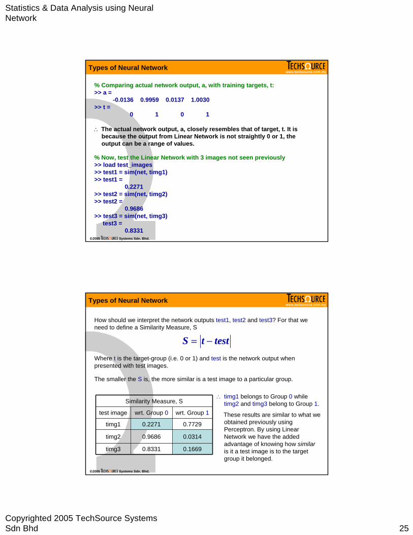
% Comparing actual network output, a, with training targets, t:>> a =

-0.0136 0.9959 0.0137 1.0030>> t =

0 1 0 1

∴ The actual network output, a, closely resembles that of target, t. It is because the output from Linear Network is not straightly 0 or 1, the output can be a range of values.

% Now, test the Linear Network with 3 images not seen previously>> load test_images>> test1 = sim(net, timg1)>> test1 =

0.2271>> test2 = sim(net, timg2)>> test2 =

0.9686>> test3 = sim(net, timg3)

test3 = 0.8331




How should we interpret the network outputs test1, test2 and test3? For that we need to define a Similarity Measure, S

S t test= −

Where t is the target-group (i.e. 0 or 1) and test is the network output when presented with test images.

0.16690.8331timg3

0.03140.9686timg2

0.77290.2271timg1

wrt. Group 1wrt. Group 0test image

Similarity Measure, S

The smaller the S is, the more similar is a test image to a particular group.

∴ timg1 belongs to Group 0 while timg2 and timg3 belong to Group 1.

These results are similar to what we obtained previously using Perceptron. By using Linear Network we have the added advantage of knowing how similar is it a test image is to the target group it belonged.






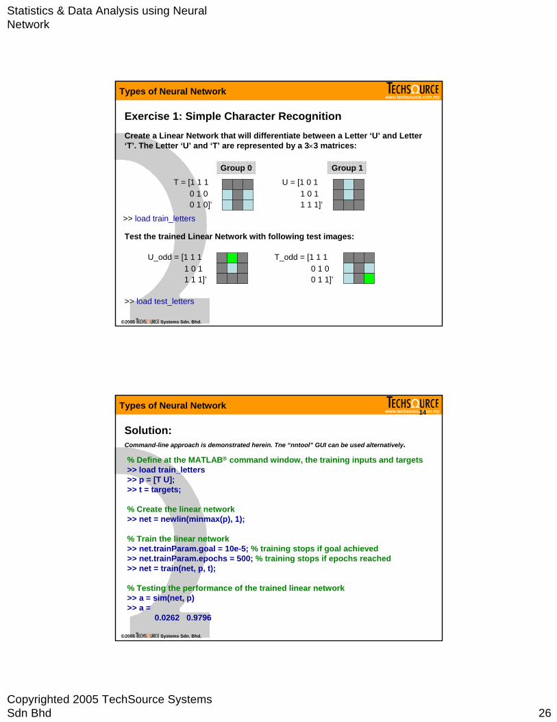
Exercise 1: Simple Character RecognitionCreate a Linear Network that will differentiate between a Letter ‘U’ and Letter ‘T’. The Letter ‘U’ and ‘T’ are represented by a 3×3 matrices:

T = [1 1 10 1 00 1 0]’

U = [1 0 11 0 11 1 1]’

Test the trained Linear Network with following test images:

U_odd = [1 1 11 0 11 1 1]’

T_odd = [1 1 10 1 00 1 1]’

>> load test_letters

>> load train_letters

Group 0 Group 1




14


% Define at the MATLAB® command window, the training inputs and targets>> load train_letters>> p = [T U];>> t = targets;

% Create the linear network>> net = newlin(minmax(p), 1);

% Train the linear network>> net.trainParam.goal = 10e-5; % training stops if goal achieved>> net.trainParam.epochs = 500; % training stops if epochs reached>> net = train(net, p, t);

% Testing the performance of the trained linear network>> a = sim(net, p)>> a =

0.0262 0.9796






15

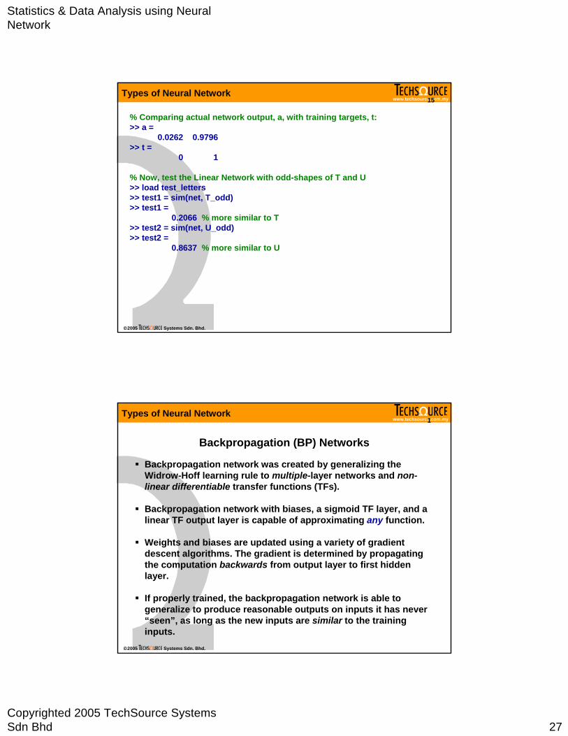
% Comparing actual network output, a, with training targets, t:>> a =

0.0262 0.9796>> t =

0 1

% Now, test the Linear Network with odd-shapes of T and U>> load test_letters>> test1 = sim(net, T_odd)>> test1 =

0.2066 % more similar to T>> test2 = sim(net, U_odd)>> test2 =

0.8637 % more similar to U




1

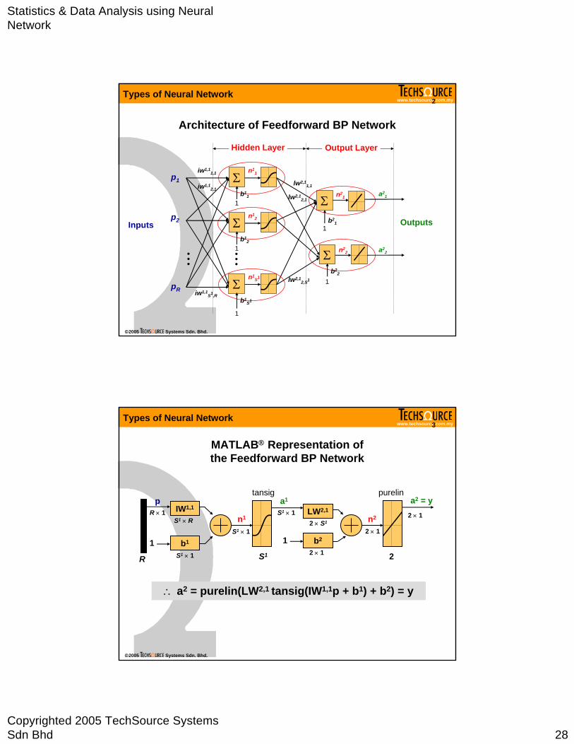
Backpropagation (BP) Networks

Backpropagation network was created by generalizing the Widrow-Hoff learning rule to multiple-layer networks and non-linear differentiable transfer functions (TFs).

Backpropagation network with biases, a sigmoid TF layer, and a linear TF output layer is capable of approximating any function.

Weights and biases are updated using a variety of gradient descent algorithms. The gradient is determined by propagating the computation backwards from output layer to first hidden layer.

If properly trained, the backpropagation network is able to generalize to produce reasonable outputs on inputs it has never “seen”, as long as the new inputs are similar to the training inputs.






2

Architecture of Feedforward BP Network

Σ

Σ

Σ

p1

p2

n11

a21

1b1

1

iw1,11,1

iw1,12,1

iw1,1S1,R

lw2,11,1

Inputs Outputs

pR Σ

Σ••••••

b12

b1S1

1

1

1

1

b21

b22

n12

n1S1

n21

n22 a2

2

lw2,12,1

lw2,12,S1

Hidden Layer Output Layer




3

MATLAB® Representation of the Feedforward BP Network

IW1,1

b1

R

R × 1p

1

S1 × R

S1 × 1

n1

S1 × 1

S1

a1

S1 × 1 LW2,1

b2

n2

2 × 1

2

a2 = y2 × 1

2 × S1

12 × 1


tansig purelin






4

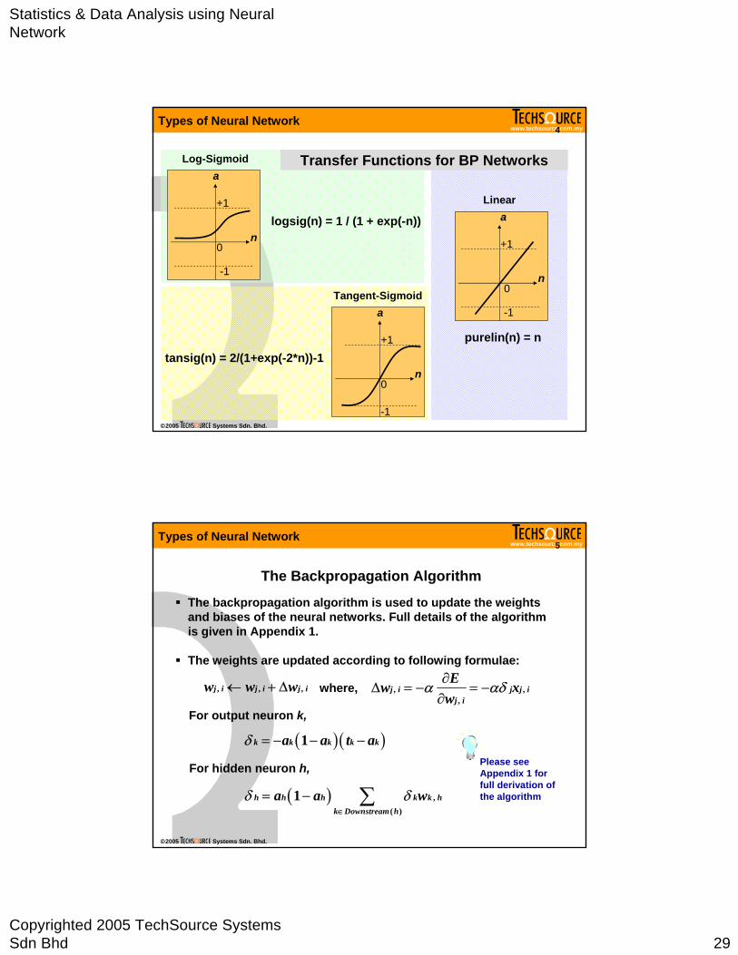
Transfer Functions for BP Networksa

0

+1

n

-1

a

0

+1

n

-1

a

0

+1

-1

n

Log-Sigmoid

Tangent-Sigmoid

Linear

logsig(n) = 1 / (1 + exp(-n))

tansig(n) = 2/(1+exp(-2*n))-1purelin(n) = n




The Backpropagation Algorithm

The backpropagation algorithm is used to update the weights and biases of the neural networks. Full details of the algorithm is given in Appendix 1.

The weights are updated according to following formulae:

5

, ,,

j i j j ij i

Ew xw

α αδ∂∆ = − = −

∂, , ,j i j i j iw w w← + ∆

( ) ( )1k k k k ka a t aδ = − − −

( ) ,( )

1h h h k k hk Downstream h

a a wδ δ∈

= − ∑

where,

For output neuron k,

For hidden neuron h, Please see Appendix 1 for full derivation of the algorithm






Training of Backpropagation Networks

6

There are generally four steps in the training process:

1. Assemble the training data;2. Create the network object;3. Train the network;4. Simulate the network response to new inputs.

The MATLAB® Neural Network Toolbox implements some of the most popular training algorithms, which encompass both original gradient-descent and faster training methods.




Batch Gradient Descent Training

7

Batch Training: the weights and biases of the network are updated only after the entire training data has been applied to the network.

Batch Gradient Descent (traingd):

• Original but the slowest;

• Weights and biases updated in the direction of the negative gradient (note: backprop. algorithm);

• Selected by setting trainFcn to traingd:

net = newff(minmax(p), [3 1], {‘tansig’, ‘purelin’}, ‘traingd’);






8

Batch Gradient Descent with Momentum

Batch Gradient Descent with Momentum (traingdm):

• Faster convergence than traingd;

• Momentum allows the network to respond not only the local gradient, but also to recent trends in the error surface;

• Momentum allows the network to ignore small features in the error surface; without momentum a network may get stuck in a shallow local minimum.

• Selected by setting trainFcn to traingdm:

net = newff(minmax(p), [3 1], {‘tansig’, ‘purelin’}, ‘traingdm’);




Faster Training

The MATLAB® Neural Network Toolbox also implements some of the faster training methods, in which the training can converge from ten to one hundred times faster than traingdand traingdm.

These faster algorithms fall into two categories:

1. Heuristic techniques: developed from the analysis of the performance of the standard gradient descent algorithm, e.g. traingda, traingdx and trainrp.

2. Numerical optimization techniques: make use of the standard optimization techniques, e.g. conjugate gradient (traincgf, traincgb, traincgp, trainscg), quasi-Newton (trainbfg, trainoss), and Levenberg-Marquardt (trainlm).






10

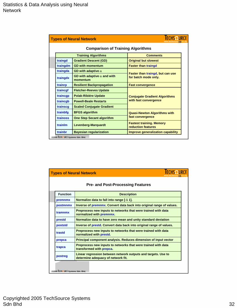
Comparison of Training Algorithms

GD with adaptive α and with momentumtraingdx

One Step Secant algorithmtrainossQuasi-Newton Algorithms with fast convergence

BFGS algorithmtrainbfg

Improve generalization capability

Fastest training. Memory reduction features

Conjugate Gradient Algorithms with fast convergence

Fast convergence

Faster than traingd, but can use for batch mode only.

Faster than traingdOriginal but slowest

Comments

Levenberg-Marquardt trainlm

Bayesian regularizationtrainbr

Scaled Conjugate GradienttrainscgPowell-Beale Restartstraincgb

Polak-Ribiére Updatetraincgp

Fletcher-Reeves UpdatetraincgfResilient Backpropagationtrainrp

GD with adaptive αtraingdaGD with momentumtraingdmGradient Descent (GD)traingd

Training Algorithms




11

Pre- and Post-Processing Features

Linear regression between network outputs and targets. Use to determine adequacy of network fit.postreg

Description

Preprocess new inputs to networks that were trained with data transformed with prepca.trapca

Principal component analysis. Reduces dimension of input vectorprepca

Preprocess new inputs to networks that were trained with data normalized with prestd.trastd

Inverse of prestd. Convert data back into original range of values.poststd

Normalize data to have zero mean and unity standard deviationprestd

Preprocess new inputs to networks that were trained with data normalized with premnmx.tramnmx

Inverse of premnmx. Convert data back into original range of values.postmnmxNormalize data to fall into range [-1 1].premnmx

Function






12

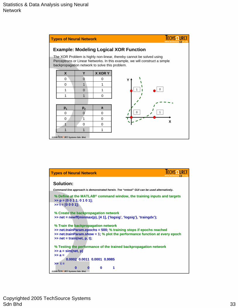
Example: Modeling Logical XOR FunctionThe XOR Problem is highly non-linear, thereby cannot be solved using Perceptrons or Linear Networks. In this example, we will construct a simple backpropagation network to solve this problem.

011101110000

X XOR YYX

0

1

1

0

X

Y

111001010000ap2p1





% Define at the MATLAB® command window, the training inputs and targets>> p = [0 0 1 1; 0 1 0 1];>> t = [0 0 0 1];

% Create the backpropagation network>> net = newff(minmax(p), [4 1], {‘logsig’, ‘logsig’}, ‘traingdx’);

% Train the backpropagation network>> net.trainParam.epochs = 500; % training stops if epochs reached>> net.trainParam.show = 1; % plot the performance function at every epoch>> net = train(net, p, t);

% Testing the performance of the trained backpropagation network>> a = sim(net, p)>> a =

0.0002 0.0011 0.0001 0.9985>> t =

0 0 0 1






14

Improving Generalization with Early Stopping

The generalization capability can be improved with the early stopping feature available with the Neural Network toolbox.

In this technique the available data is divided into three subsets:

1. Training set2. Validation set3. Testing set

The early stopping feature can be invoked when using the train command:

[net, tr] = train(net, p, t, [ ], [ ], VV, TV)

VV: Validation set structure; TV: Test set structure.




15

Example: Function Approximation with Early Stopping

% Define at the MATLAB® command window, the training inputs and targets>> p = [-1: 0.05: 1];>> t = sin(2*pi*p) + 0.1*randn(size(p));

% Construct Validation set>> val.P = [-0.975: 0.05: 0.975]; % validation set must be in structure form>> val.T = sin(2*pi*val.P) + 0.1*randn(size(val.P));

% Construct Test set (optional)>> test.P = [-1.025: 0.05: 1.025]; % validation set must be in structure form>> test.T = sin(2*pi*test.P) + 0.1*randn(size(test.P));

% Plot and compare three data sets>> plot(p, t), hold on, plot(val.P, val.T,‘r:*’), hold on, plot(test.P, test.T, ‘k:^’); >> legend(‘train’, ‘validate’, ‘test’);

% Create a 1-20-1 backpropagation network with ‘trainlm’ algorithm>> net = newff(minmax(p), [20 1], {‘tansig’, ‘purelin’}, ‘trainlm’);






16

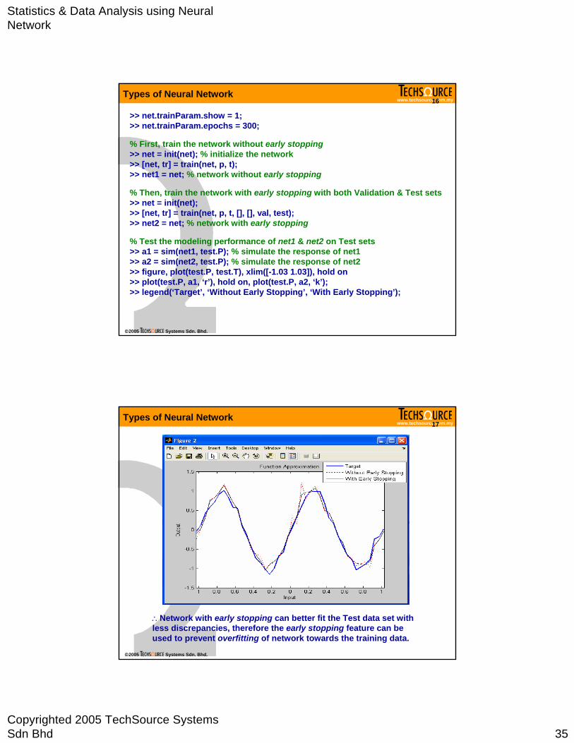
>> net.trainParam.show = 1;>> net.trainParam.epochs = 300;

% First, train the network without early stopping>> net = init(net); % initialize the network>> [net, tr] = train(net, p, t);>> net1 = net; % network without early stopping

% Then, train the network with early stopping with both Validation & Test sets>> net = init(net);>> [net, tr] = train(net, p, t, [], [], val, test);>> net2 = net; % network with early stopping

% Test the modeling performance of net1 & net2 on Test sets>> a1 = sim(net1, test.P); % simulate the response of net1>> a2 = sim(net2, test.P); % simulate the response of net2>> figure, plot(test.P, test.T), xlim([-1.03 1.03]), hold on>> plot(test.P, a1, ‘r’), hold on, plot(test.P, a2, ‘k’);>> legend(‘Target’, ‘Without Early Stopping’, ‘With Early Stopping’);




17

∴Network with early stopping can better fit the Test data set with less discrepancies, therefore the early stopping feature can be used to prevent overfitting of network towards the training data.






18

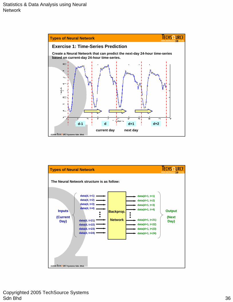
Exercise 1: Time-Series Prediction Create a Neural Network that can predict the next-day 24-hour time-series based on current-day 24-hour time-series.

dd-1 d+1 d+2

current day next day




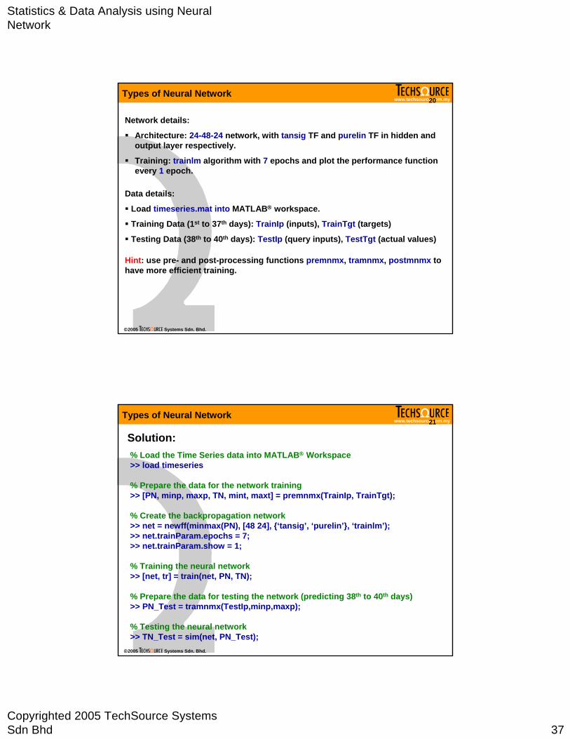
19

The Neural Network structure is as follow:

Backprop.

Network

data(d, t=1)data(d, t=2)data(d, t=3)data(d, t=4)

data(d, t=21)data(d, t=22)data(d, t=23)data(d, t=24)

Inputs

(Current Day)

data(d+1, t=1)data(d+1, t=2)data(d+1, t=3)data(d+1, t=4)

data(d+1, t=21)data(d+1, t=22)data(d+1, t=23)data(d+1, t=24)

Output

(Next Day)






20

Data details:

Load timeseries.mat into MATLAB® workspace.

Training Data (1st to 37th days): TrainIp (inputs), TrainTgt (targets)

Testing Data (38th to 40th days): TestIp (query inputs), TestTgt (actual values)

Network details:

Architecture: 24-48-24 network, with tansig TF and purelin TF in hidden and output layer respectively.

Training: trainlm algorithm with 7 epochs and plot the performance function every 1 epoch.

Hint: use pre- and post-processing functions premnmx, tramnmx, postmnmx to have more efficient training.




21

Solution:% Load the Time Series data into MATLAB® Workspace>> load timeseries

% Prepare the data for the network training>> [PN, minp, maxp, TN, mint, maxt] = premnmx(TrainIp, TrainTgt);

% Create the backpropagation network>> net = newff(minmax(PN), [48 24], {‘tansig’, ‘purelin’}, ‘trainlm’);>> net.trainParam.epochs = 7;>> net.trainParam.show = 1;

% Training the neural network>> [net, tr] = train(net, PN, TN);

% Prepare the data for testing the network (predicting 38th to 40th days) >> PN_Test = tramnmx(TestIp,minp,maxp);

% Testing the neural network>> TN_Test = sim(net, PN_Test);






22

% Convert the testing output into prediction values for comparison purpose >> [queryInputs predictOutputs] = postmnmx(PN_Test, minp, maxp, …TN_Test, mint, maxt);

% Plot and compare the predicted and actual time series>> predictedData = reshape(predictOutputs, 1, 72);>> actualData = reshape(TestTgt, 1, 72);>> plot(actualData, ‘-*’), hold on>> plot(predictOutputs, ‘r:’);




23

Homework: Try to subdivide the training data [TrainIp TrainTgt] into Training & Validation Sets to accertain whether the use of early stopping would improve the prediction accuracy.






24

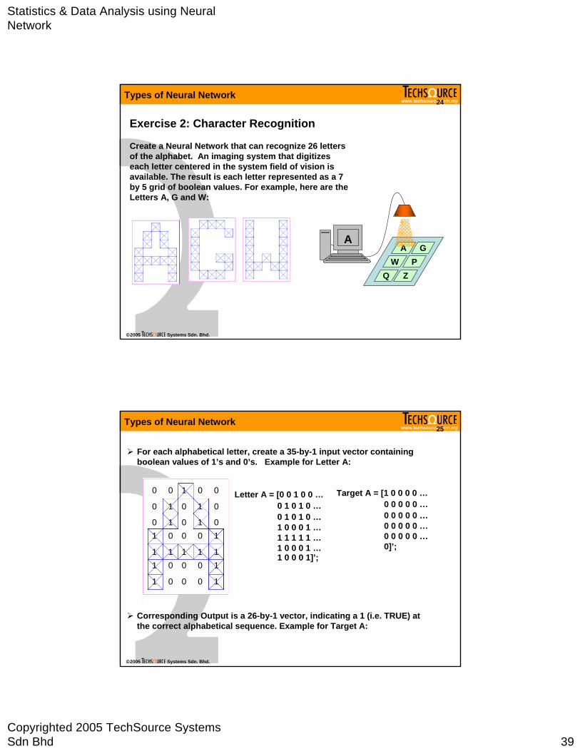
Exercise 2: Character Recognition

Create a Neural Network that can recognize 26 letters of the alphabet. An imaging system that digitizes each letter centered in the system field of vision is available. The result is each letter represented as a 7 by 5 grid of boolean values. For example, here are the Letters A, G and W:

A GW P

Q Z

A




For each alphabetical letter, create a 35-by-1 input vector containing boolean values of 1’s and 0’s. Example for Letter A:

0 0 1 0 0

0 1 0 1 0

0 1 0 1 01 0 0 0 1

1 1 1 1 11 0 0 0 1

1 0 0 0 1

Letter A = [0 0 1 0 0 …0 1 0 1 0 …0 1 0 1 0 …1 0 0 0 1 …1 1 1 1 1 …1 0 0 0 1 …1 0 0 0 1]’;

Corresponding Output is a 26-by-1 vector, indicating a 1 (i.e. TRUE) at the correct alphabetical sequence. Example for Target A:

Target A = [1 0 0 0 0 …0 0 0 0 0 …0 0 0 0 0 …0 0 0 0 0 …0 0 0 0 0 …0]’;






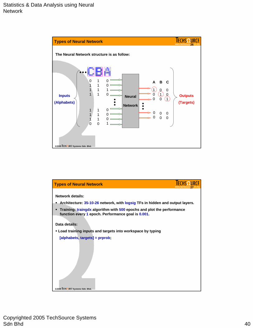
The Neural Network structure is as follow:

Neural

Network

0010

0001

1111

1110

1110

0111

100

00

010

00

00

001

A B C

Inputs

(Alphabets)

Outputs

(Targets)




Data details:

Load training inputs and targets into workspace by typing

[alphabets, targets] = prprob;

Network details:

Architecture: 35-10-26 network, with logsig TFs in hidden and output layers.

Training: traingdx algorithm with 500 epochs and plot the performance function every 1 epoch. Performance goal is 0.001.






Solution:% Load the training data into MATLAB® Workspace>> [alphabets, targets] = prprob;

% Create the backpropagation network>> net = newff(minmax(alphabets), [10 26], {‘logsig’, ‘logsig’}, ‘traingdx’);>> net.trainParam.epochs = 500;>> net.trainParam.show = 1;>> net.trainParam.goal = 0.001;

% Training the neural network>> [net, tr] = train(net, alphabets, targets);

% First, we create a normal ‘J’ to test the network performance>> J = alphabets(:,10);>> figure, plotchar(J);>> output = sim(net, J);>> output = compet(output) % change the largest values to 1, the rest 0s>> answer = find(compet(output) == 1); % find the index (out of 26) of network output>> figure, plotchar(alphabets(:, answer));




29

% Next, we create a noisy ‘J’ to test the network can still identify it correctly…>> noisyJ = alphabets(:,10)+randn(35,1)*0.2;>> figure; plotchar(noisyJ);>> output2 = sim(network1, noisyJ);>> output2 = compet(output2);>> answer2 = find(compet(output2) == 1);>> figure; plotchar(alphabets(:,answer2));






1

Self-Organizing Maps

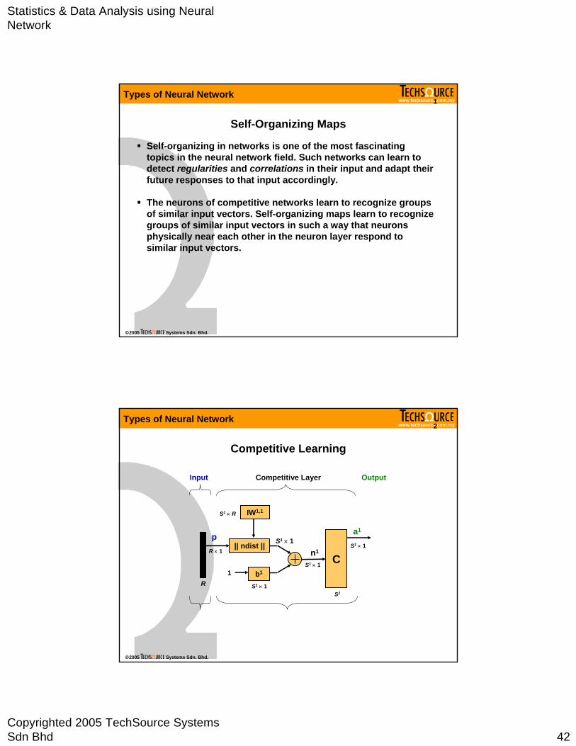
Self-organizing in networks is one of the most fascinating topics in the neural network field. Such networks can learn to detect regularities and correlations in their input and adapt their future responses to that input accordingly.

The neurons of competitive networks learn to recognize groups of similar input vectors. Self-organizing maps learn to recognize groups of similar input vectors in such a way that neurons physically near each other in the neuron layer respond to similar input vectors.




2

Competitive Learning

IW1,1

b1

C

R

Output

R × 1

p

1

S1 × R

S1 × 1

n1

S1 × 1

S1

a1

S1 × 1

Input Competitive Layer

|| ndist || S1 × 1






3

Learning Algorithms for Competitive Network

The weights of the winning neuron (represented by a row of the input weight matrix) are adjusted with the Kohonen learning rule (learnk).

Supposed that the ith neuron wins, the elements of the ith row of the input weight matrix are adjusted according to following formula:

iIW1,1(q) = iIW1,1(q-1) + α(p(q) – iIW1,1(q-1))

One of the limitations of the competitive networks is that some neurons may never wins because their weights are far from any input vectors.

The bias learning rule (learncon) is used to allow every neuron in the network learning from the input vectors.




4

Example: Classification using Competitive Network

p(1)

p(2)

We can use a competitive network to classify input vectors without any learning targets.

Let’s say if we create four two-element input vectors, with two very close to (0 0) and others close to (1 1).

p = [0.1 0.8 0.1 0.9

0.2 0.9 0.1 0.8];

Let’s see whether the competitive network is able to identify the classification structure…






5

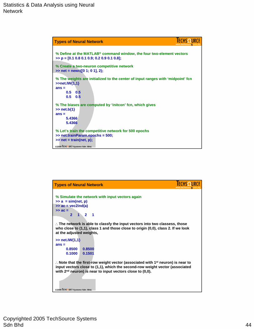
% Define at the MATLAB® command window, the four two-element vectors>> p = [0.1 0.8 0.1 0.9; 0.2 0.9 0.1 0.8];

% Create a two-neuron competitive network>> net = newc([0 1; 0 1], 2);

% The weights are initialized to the center of input ranges with ‘midpoint’ fcn>>net.IW{1,1}ans =

0.5 0.50.5 0.5

% The biases are computed by ‘initcon’ fcn, which gives>> net.b{1}ans =

5.43665.4366

% Let’s train the competitive network for 500 epochs>> net.trainParam.epochs = 500;>> net = train(net, p);




6

% Simulate the network with input vectors again>> a = sim(net, p)>> ac = vec2ind(a)>> ac =

2 1 2 1

∴The network is able to classfy the input vectors into two classess, those who close to (1,1), class 1 and those close to origin (0,0), class 2. If we look at the adjusted weights,

>> net.IW{1,1}ans =

0.8500 0.85000.1000 0.1501

∴Note that the first-row weight vector (associated with 1st neuron) is near to input vectors close to (1,1), which the second-row weight vector (associated with 2nd neuron) is near to input vectors close to (0,0).






7

Exercise 1: Classification of Input Vectors:Graphical Example

First, generate the input vectors by using the built-in nngenc function:

>> X = [0 1; 0 1]; % Cluster centers to be in these bounds>> clusters = 8; % Number of clusters>> points = 10; % Number of points in each cluster>> std_dev = 0.05; % Standard deviation of each cluster>> P = nngenc(X,clusters,points,std_dev); % Number of clusters

Plot and show the generated clusters

>> plot(P(1,:),P(2,:),'+r');>> title('Input Vectors');>> xlabel('p(1)');>> ylabel('p(2)');

Try to build a competitive network with 8 neurons and train for 1000 epochs. Superimpose the trained network weights onto the same figure. Try to experiement with the number of neurons and conclude on the accuracy of the classification.




8

Solution:% Create and train the competitive network>> net = newc([0 1; 0 1], 8, 0.1); % Learning rate is set to 0.1>> net.trainParam.epochs = 1000;>> net = train(net, P);

% Plot and compare the input vectors and cluster centres determined by the competitive network>> w = net.IW{1,1};>> figure, plot(P(1,:),P(2,:),‘+r’);>> hold on, plot(w(:,1), w(:,2), ‘ob’);

% Simulate the trained network to new inputs>> t1 = [0.1; 0.1], t2 = [0.35; 0.4], t3 = [0.8; 0.2];>> a1 = sim(net, [t1 t2 t3]);>> ac1 = vec2ind(a1);ac1 =

1 5 6

Homework: Try altering the number of neurons in the competitive layer and observe how it affects the cluster centres.






9

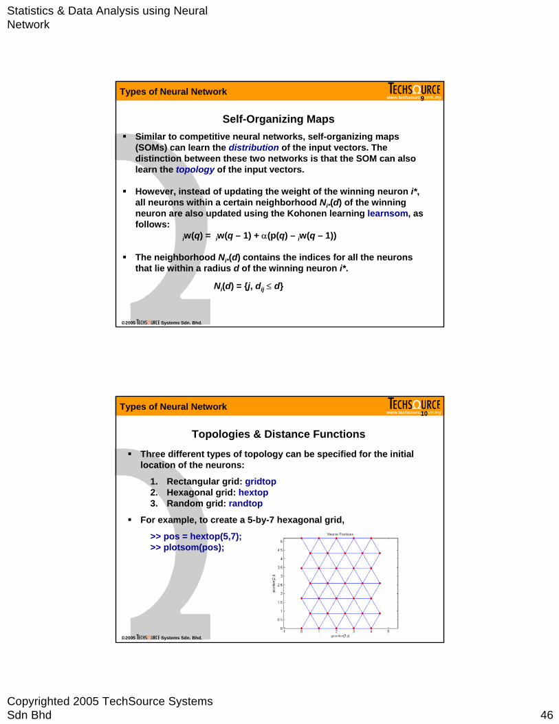
Self-Organizing MapsSimilar to competitive neural networks, self-organizing maps (SOMs) can learn the distribution of the input vectors. The distinction between these two networks is that the SOM can also learn the topology of the input vectors.

However, instead of updating the weight of the winning neuron i*, all neurons within a certain neighborhood Ni*(d) of the winning neuron are also updated using the Kohonen learning learnsom, as follows:

iw(q) = iw(q – 1) + α(p(q) – iw(q – 1))

The neighborhood Ni*(d) contains the indices for all the neurons that lie within a radius d of the winning neuron i*.

Ni(d) = {j, dij ≤ d}




10

Topologies & Distance Functions

Three different types of topology can be specified for the initial location of the neurons:

1. Rectangular grid: gridtop2. Hexagonal grid: hextop3. Random grid: randtop

For example, to create a 5-by-7 hexagonal grid,

>> pos = hextop(5,7);>> plotsom(pos);






11

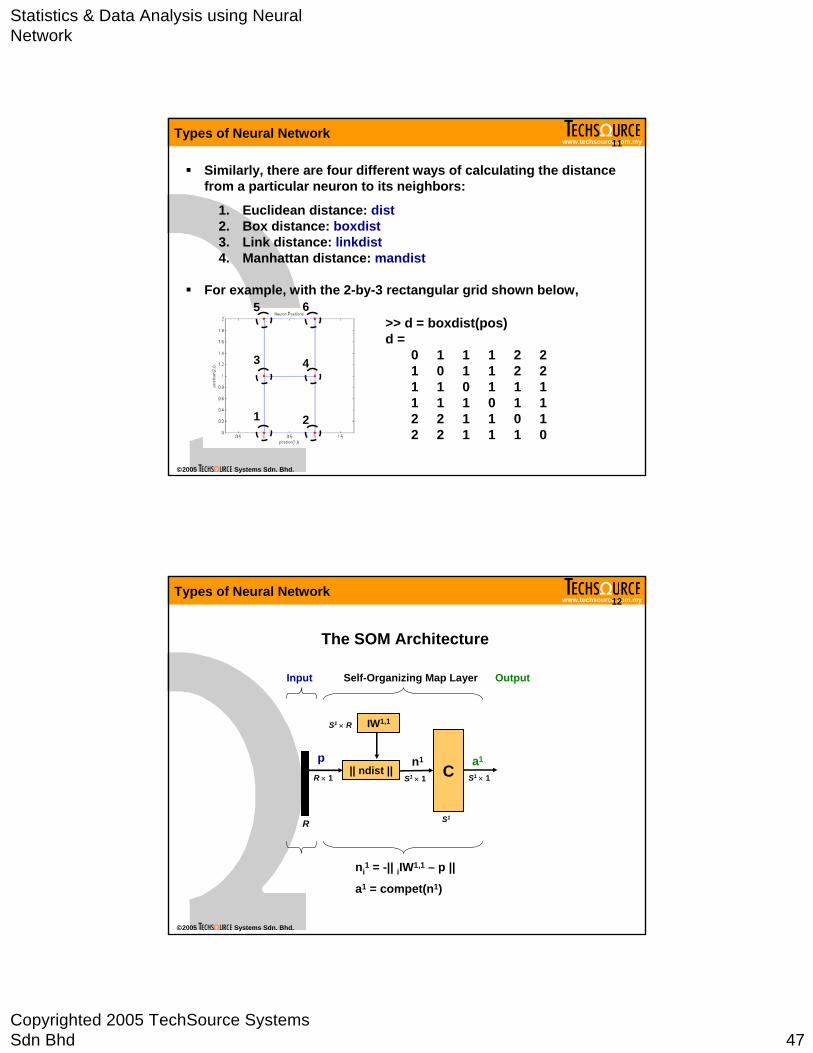
Similarly, there are four different ways of calculating the distance from a particular neuron to its neighbors:

1. Euclidean distance: dist2. Box distance: boxdist3. Link distance: linkdist4. Manhattan distance: mandist

For example, with the 2-by-3 rectangular grid shown below,

>> d = boxdist(pos)d =

0 1 1 1 2 21 0 1 1 2 21 1 0 1 1 11 1 1 0 1 12 2 1 1 0 12 2 1 1 1 0

1 2

3 4

5 6




12

The SOM Architecture

IW1,1

C

R

Output

R × 1

p

S1 × R

n1

S1 × 1

S1

a1

Input Self-Organizing Map Layer

|| ndist ||S1 × 1

ni1 = -|| iIW1,1 – p ||

a1 = compet(n1)






13

Creating and Training the SOM

Let’s load an input vector into MATLAB® workspace>> load somdata>> plot(P(1,:), P(2,:), ‘g.’, ‘markersize’, 20), hold on

Create a 2-by-3 SOM with following command, and superimpose the initial weights onto the input space>> net = newsom([0 2; 0 1], [2 3]);>> plotsom(net.iw{1,1}, net.layers{1}.distances), hold off

The weights of the SOM are updated using the learnsom function, where the winning neuron’s weights are updated proportional to αand the weights of neurons in its neighbourhood are altered proportional to ½ of α.




14

The training is divided into two phases:

1. Ordering phase: The neighborhood distance starts as the maximum distance between two neurons, and decreases to the tuning neighborhood distance. The learning rate starts at the ordering-phase learning rate and decreases until it reaches the tuning-phase learning rate. This phase typically allows the SOM to learn the topology of the input space.

2. Tuning Phase: The neighborhood distance stays at the tuning neighborhood distance (i.e., typically 1.0). The learning rate continues to decrease from the tuning phase learning rate, but very slowly. The small neighborhood and slowly decreasing learning rate allows the SOM to learn the distribution of the input space. The number of epochs for this phase should be much larger than the number of steps in the ordering phase.






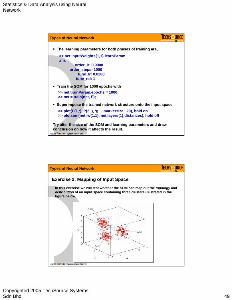
The learning parameters for both phases of training are,

>> net.inputWeights{1,1}.learnParamans =

order_lr: 0.9000order_steps: 1000

tune_lr: 0.0200tune_nd: 1

Train the SOM for 1000 epochs with>> net.trainParam.epochs = 1000;>> net = train(net, P);

Superimpose the trained network structure onto the input space>> plot(P(1,:), P(2,:), ‘g.’, ‘markersize’, 20), hold on>> plotsom(net.iw{1,1}, net.layers{1}.distances), hold off

Try alter the size of the SOM and learning parameters and draw conclusion on how it affects the result.




Exercise 2: Mapping of Input Space

16

In this exercise we will test whether the SOM can map out the topology and distribution of an input space containing three clusters illustrated in the figure below,






17

Solution:% Let’s start by creating the data for the input space illustrated previously

>> d1 = randn(3,100); % cluster center at (0, 0, 0)>> d2 = randn(3, 100) + 3; % cluster center at (3, 3, 3)>> d3 = randn(3,100), d3(1,:) = d3(1,:) + 9; % cluster center at (9, 0, 0)>> d = [d1 d2 d3];

% Plot and show the generated clusters

>> plot3(d(1,:), d(2,:), d(3,:), ‘ko’), hold on, box on

% Try to build a 10-by-10 SOM and train it for 1000 epochs,>> net = newsom(minmax(d), [10 10]);>> net.trainParam.epochs = 1000;>> net = train(net, d);

% Superimpose the trained SOM’s weights onto the input space,>> gcf, plotsom(net.IW{1,1}, net.layers{1}.distances), hold off

% Simulate SOM to get indices of neurons closest to input vectors>> A = sim(net, d), A = vec2ind(A);





Section Summary:1. Perceptrons

IntroductionThe perceptron architectureTraining of perceptronsApplication examples

2. Linear NetworksIntroductionArchitecture of linear networksThe Widrow-Hoff learning algorithmApplication examples

3. Backpropagation NetworksIntroductionArchitecture of backprogation networkThe backpropagation algorithmTraining algorithmsPre- and post-processingApplication examples

4. Self-Organizing MapsIntroductionCompetitive learningSelf-organizing mapsApplication examples





Case Study

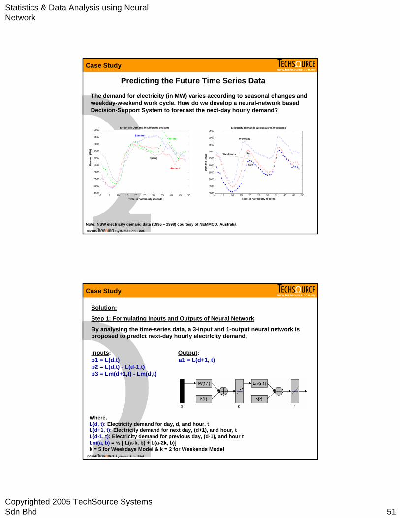
Predicting the Future Time Series Data

The demand for electricity (in MW) varies according to seasonal changes and weekday-weekend work cycle. How do we develop a neural-network based Decision-Support System to forecast the next-day hourly demand?

0 5 10 15 20 25 30 35 40 45 504500

5000

5500

6000

6500

7000

7500

8000

8500

9000Electricity Demand in Different Seasons

Time in half-hourly records

Dem

and

(MW

)

Summer

Autumn

Winter

Spring

0 5 10 15 20 25 30 35 40 45 505000

5500

6000

6500

7000

7500

8000

8500

9000

9500Electricity Demand: Weekdays Vs Weekends

Time in half-hourly records

Dem

and

(MW

)

Weekday

Sat

Sun

Weekends

Note: NSW electricity demand data (1996 – 1998) courtesy of NEMMCO, Australia



Case Study

Solution:

Step 1: Formulating Inputs and Outputs of Neural Network

By analysing the time-series data, a 3-input and 1-output neural network is proposed to predict next-day hourly electricity demand,

Inputs: Output:p1 = L(d,t) a1 = L(d+1, t)p2 = L(d,t) - L(d-1,t)p3 = Lm(d+1,t) - Lm(d,t)

Where,L(d, t): Electricity demand for day, d, and hour, tL(d+1, t): Electricity demand for next day, (d+1), and hour, t L(d-1, t): Electricity demand for previous day, (d-1), and hour tLm(a, b) = ½ [ L(a-k, b) + L(a-2k, b)]k = 5 for Weekdays Model & k = 2 for Weekends Model





Case Study

Step 2: Pre-process Time Series Data to Appropriate Format

The time-series data is in MS Excel format and was date- and time-tagged. We need to preprocess the data according to following steps:

1. Read from the MS Excel file [histDataIp.m]

2. Divide the data into weekdays and weekends [divideDay.m]

3. Remove any outliers from the data [outlierRemove.m]

Step 3: Constructing Inputs and Output Data for Neural Network

Arrange the processed data in accordance to neural-network format:

1. Construct Input-Output pair [nextDayIp.m]

2. Normalizing the training data for faster learning [processIp.m]

Step 4: Training & Testing the Neural Network

Train the neural network using command-line or NNTOOL. When training is completed, proceed to test the robustness of the network against “unseen”data.



The EndThe EndKindly return your Evaluation Form

Tel: 603 Tel: 603 –– 8076 1953 Fax: 603 8076 1953 Fax: 603 –– 8076 19548076 1954Email: Email: [email protected]@techsource.com.my Web: Web: www.techsource.com.mywww.techsource.com.myTechTech--Support: Support: [email protected]@techsource.com.my

Statistical & Data Analysis Using Neural Network · · 2015-03-12Statistical & Data Analysis...

Documents

Transcript of Statistical & Data Analysis Using Neural Network · · 2015-03-12Statistical & Data Analysis...