© 2006 McGraw-Hill Higher Education. All rights reserved. Chapter 2 Describing and Presenting a...

© 2006 McGraw-Hill Higher Education. All rights reserved.

Chapter 2

Describing and Presenting a Distribution of Scores


Chapter 2


Chapter Objectives

After completing this chapter, you should be able to

1. Define all statistical terms that are presented.2. Describe the four scales of measurement and provide

examples of each.3. Describe a normal distribution and four curves for

distributions that are not normal.4. Define the terms measures of central tendency and

measures of variability.5. Define the three measures of central tendency, identify

the symbols used to represent them, describe their characteristics, calculate them with ungrouped and grouped data, and state how they can be used to interpret data.


Chapter Objectives

6. Define the three measures of variability, identify the symbols used to represent them, describe their characteristics, calculate them with ungrouped and grouped data, and state how they can be used to interpret data.

7. Define percentile and percentile rank, identify the symbols used to represent them, calculate them with ungrouped and grouped date, and state how they can be used to interpret data.

8. Define standard scores, calculate z-scores, and interpret their meanings.


Statistical Terms

• data• variable• population• sample• random sample• parameter• Statistic

• descriptive statistics• inferential statistics• discrete data• continuous data• ungrouped data• grouped data


Numbers

• Numbers mean different things in different situations. Consider three answers that appear to be identical but are not.

• “What number were you wearing in the race?” “5”

• What place did you finish in ?” “5”

• How many minutes did it take you to finish?” “5”


Number Scales

• Nominal Scale

• Ordinal Scale

• Interval

• Ratio


Nominal Scale: This scale refers to a classificatory approach, i.e.,

categorizing observations. Distinct characteristics must exist to

categorize: gender, race essentially you can only be assigned one

group. KEY: to distinguish one from another.


Ordinal Scale: This scale puts order into categories. It only ranks categories by

ability, but there is no specific quantification between categories. It is only placement, e.g., judging a swimming race without a stopwatch, i.e., there is no quantitiy to

determine the difference between ranks. KEY: placement without quantification.


Interval Scale: This scale adds equal intervals between observed categories. We

know that 75 points is halfway between scores of 70 and 80 points on a scale. KEY:

how much was the difference between 1st and 2nd place?


Ratio Scale: this scale has all the qualities of an interval scale with the added property of a true zero.

Not all qualities can be assigned to a ratio scale. KEY: quality of

measurement must represent a true zero.


Normal Distribution

• Most statistical methods are based on assumption that a distribution of scores is normal and that the distribution can be graphically represented by the normal curve (bell-shaped).

• Normal distribution is theoretical and is based on the assumption that the distribution contains an infinite number of scores.


Characteristics of Normal Curve

• Bell-shaped curve

• Symmetrical distribution about vertical axis of curve

• Greatest number of scores found in middle of curve

• All measures of central tendency at vertical axis


meanmedianmode


Different Curves

• leptokurtic - very homogeneous group

• platykurtic - very heterogeneous group

• bimodal - two high points

• skewed - scores clustered at one end; positive or negative


Score Rank

1. List scores in descending order.

2. Number the scores; highest score is number 1 and last score is the number of the total number of scores.

3. Average rank of identical scores and assign them the same rank (may determine the midpoint and assign that rank).


Table 2.2 Rank of Volleyball Knowledge Test Scores

Rank Score Rank Score1 96 16 16 882 95 17 883 93 18 884 4.5 92 19 875 92 20 20 876 6.5 91 21 877 91 22 22.5 868 90 23 869 9 90 24 24.5 85

10 90 25 8511 89 26 26.5 8412 12 89 27 8413 89 28 8314 88 29 8215 88 30 81


Measures of Central Tendency

• descriptive statistics

• describe the middle characteristics of the data (distribution of scores); represent scores in a distribution around which other scores seem to center

• most widely used statistics

• mean, median, and mode


Mean

The arithmetic average of a distribution of scores; most generally used measure of central tendency.

Characteristics• Most sensitive of all measures of central tendency• Most appropriate measure of central tendency to use for

ratio data (may be used on interval data)• Considers all information about the data and is used to

perform other statistical calculations• Influenced by extreme scores, especially if the

distribution is small


Symbols Used to Calculate Mean

X = the mean (called X-bar)

= (Greek letter sigma) = “the sum of”

X = individual score

N = the total number of scores in distribution Mean Formula X = X

N

Table 2.3: X = 2644 = 88.1

30


Median

Score that represents the exact middle of the distribution; the fiftieth percentile; the score that 50% of the scores are above and 50% of the scores are below.

Characteristics• Not affected by extreme scores.• A measure of position.• Not used for additional statistical calculations.

• Represented by Mdn or P50.


Steps in Calculation of Median

1. Arrange the scores in ascending order.2. Multiple N by .50.3. If the number of scores is odd, P50 is the

middle score of the distribution.4. If the number of scores is even, P50 is the

arithmetic average of the two middle scores of the distribution.

Table 2.3: .50(30) = 15 Fifteenth and sixteenth scores are 88 P50 = 88


Mode

Score that occurs most frequently; may have more than one mode.

Characteristics Least used measure of central tendency. Not used for additional statistics. Not affected by extreme scores.

Table 2.3: Mode = 88


Which Measure of Central Tendency is Best for Interpretation of Test Results?

• Mean, median, and mode are the same for a normal distribution, but often will not have a normal curve.

• The farther away from the mean and median the mode is, the less normal the distribution.

• The mean and median are both useful measures.

• In most testing, the mean is the most reliable and useful measure of central tendency; it is also used in many other statistical procedures.


Measures of Variability

• To provide a more meaningful interpretation of data, you need to know how the scores spread.

• Variability - the spread, or scatter, of scores; terms dispersion and deviation often used

• With the measures of variability, you can determine the amount that the scores spread, or deviate, from the measures of central tendency.

• Descriptive statistics; reported with measures of central tendency


Range

Determined by subtracting the lowest score from the highest score; represents on the extreme scores.

Characteristics1. Dependent on the two extreme scores.2. Least useful measure of variability.

Formula: R = Hx - Lx

Table 2.3: R = 96 - 81 = 15


Quartile Deviation

Sometimes called semiquartile range; is the spread of middle 50% of the scores around the median. Extremescores will not affect the quartile deviation.

Characteristics1. Uses the 75th and 25th percentiles; difference between these two percentiles is referred to as the interquartile range.2. Indicates the amount that needs to be added to, and subtracted from, the median to include the middle 50% of the scores.3. Usually not used in additional statistical calculations.


Quartile Deviation

Symbols

Q = quartile deviation

Q1 = 25th percentile or first quartile (P25) = score in which 25% of scores are below and 75% of scores are above

Q3 = 75th percentile or third quartile (P75) = score in which 75% of scores are below and 25% of scores are above


Steps for Calculation of Q3

1. Arrange scores in ascending order.2. Multiply N by .75 to find 75% of the distribution.3. Count up from the bottom score to the number determined in step 2. Approximation and interpolation may be required.Steps for Calculation of Q1

1. Multiply N by .25 to find 25% of the distribution.2. Count up from the bottom score to the number determined in step 1.

To Calculate QSubstitute values in formula: Q = Q3 - Q1

2


Quartiles

Q1 = 25%

Q2 = 50%

Q3 = 75%

Q4 = 100%

Q2 - Q1 = range of scores below median

Q3 - Q2 = range of scores above median


Table 2.3: 1. .75(30) = 22.5; twenty-second score = 90; twenty-third

score = 90; midway between two scores would be

same score 75% = 90 2. .25(30) = 7.5; seventh score = 85; eight score = 86; midway between two scores = 85.53. Q = 90 - 85.5 = 4.5 = 2.25 2 2Table 2.3: 88 + 2.25 = 90.2588 - 2.25 = 85.75 Theoretically, middle 50% of scores fall between the

scores of 85.75 and 90.25.


Standard Deviation

• Most useful and sophisticated measure of variability.• Describes the scatter of scores around the mean.• Is a more stable measure of variability than the range or

quartile deviation because it depends on the weight of each score in the distribution.

• Lowercase Greek letter sigma is used to indicate the the standard deviation of a population; letter s is used to indicate the standard deviation of a sample.

• Since you generally will be working with small samples, the formula for determining the standard deviation will include (N - 1) rather than N.


Characteristics of Standard Deviation

1. Is the square root of the variance, which is the average of the squared deviations from the mean. Population variance is represented as F2 and the sample variance is represented as s2.

2. Is applicable to interval and ratio data, includes all scores, and is the most reliable measure of variability.3. Is used with the mean. In a normal distribution, one standard deviation added to the mean and one standard deviation subtracted from the mean includes the middle 68.26% of the scores.


Characteristics of Standard Deviation4. With most data, a relatively small standard deviation indicates that the group being tested has little variability (performed homogeneously). A relatively large standard deviation indicates the group has much variability (performed heterogeneously).5. Is used to perform other statistical calculations.

Symbols used to determine the standard deviation:s = standard deviation X = individual scoreX = mean N = number of scores = sum ofd = deviation score (X - X)


Calculation of Standard Deviation with X2

1. Arrange scores into a series.2. Find X2.3. Square each of the scores and add to determine the X2.4. Insert the values into the formula

NX2 - (X)2

s = N(N- 1)

Table 2.3:X = 2644 N = 30X2 = 233,398 s = 3.6


Calculation of Standard Deviation with d2

1. Arrange the scores into a series.2. Calculate X.3. Determine d and d2 for each score; calculate d2.4. Insert the values into the formula d2

s = N - 1Table 2.4: X = 88.1 s = 3.6 d2 = 373.5 N = 30


Interpretation of Standard Deviation in Tables 2.3 and 2.4

S = 3.6X = 88.188.1 + 3.6 = 91.788.1 - 3.6 = 84.5

In a normal distribution, 68.26% of the scores would fall between 84.5 and 91.7.


Relationship of Standard Deviation and Normal Curve

Based on the probability of a normal distribution, there isan exact relationship between the standard deviation andthe proportion of area and scores under the curve.1. 68.26% of the scores will fall between +1.0 and -1.0 standard deviations.2. 95.44% of the scores will fall between +2.00 and -2.00 standard deviations.3. 99.73% of the scores will fall between +3.0 and -3.00 standard deviations.4. Generally, scores will not exceed +3.0 and -3.0 standard deviations from the mean.


Figure 2.4 Characteristics of normal curve.


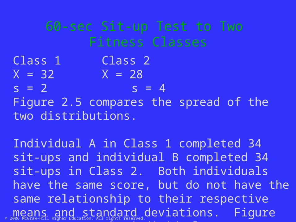
60-sec Sit-up Test to Two Fitness Classes

Class 1 Class 2X = 32 X = 28s = 2 s = 4Figure 2.5 compares the spread of the two distributions.

Individual A in Class 1 completed 34 sit-ups and individual B completed 34 sit-ups in Class 2. Both individuals have the same score, but do not have the same relationship to their respective means and standard deviations. Figure 2.6 compares the individual performances.


Calculation of Percentile Rank through Use of Mean and Standard Deviation.

1. Calculate the deviation of the score from the mean. d = (X - X)2. Calculate the number of standard deviation units the score is from the mean (z-scores). No. of standard deviation units from the mean = d s 3. Use table 2.5 to determine where the percentile rank of the score is on the curve. If negative value found in step 1, the percentile rank will always be less than 50.


Which Measure of Variability is Best forInterpretation of Test Results?

1. Range is the least desirable.2. The quartile deviation is more meaningful than the range, but it considers only the middle 50% of the scores.3. The standard deviation considers every score, is the most reliable, and is the most commonly used measure of variability.


Percentiles and Percentile Ranks

Percentile - a point in a distribution of scores belowwhich a given percentage of scores fall.Examples - 60th percentile and 40 percentile

Percentile rank - percentage of the total scores that fall below a given score in a distribution; determined by beginning with the raw scores and calculating the percentile ranks for the scores.


Weakness of Percentiles

1. The relative distance between percentile scores are the same, but the relative distances between the observed scores

are not.2. Since percentile scores are based on the number of scores in a

distribution rather than the size of the score obtained, it is sometimes more difficult to increase a percentile score at the ends of the scale than in in the middle.

3. Average performers (in middle of distribution) need only a small change in their raw scores to produce a large change in their percentile scores.

4. Below average and above average performers (at ends of distribution) need a large change in their raw scores to produce even a small change in their percentile scores.


Analysis of Grouped Data

Frequency distribution – method for arranging the data in aMore convenient form.

Simple frequency distribution – all scores are listed in Descending order and the number of times each individualScores occurs is indicated in a frequency column. Table 2.6 shows a simple frequency distribution.

Sometimes more convenient to represent scores in a groupedfrequency distribution.


Tennis Serve Test Scores

88 83 75 81 56 82 86 62 87 79 93 58 61 61 7589 94 48 79 72 81 85 52 73 62 80 73 84 63 6190 63 75 73 67 72 73 72 77 73 85 82 70 57 5891 79 68 54 70 77 81 68 83 65 77 90 52 75 6284 69 56 68 69 63 70 91 70 80 65 70 88 72 63


Steps to Construct Frequency Distribution

Step 1. Determine the range. The highest score minus lowest score. 94 – 48 = 46

Step 2. Determine the number of class intervals. Depends on the number of scores, the range of the scores, and the purpose of organizing the frequency table.

Generally it is best to have between 10 and 20 intervals.



Determine the size of the class interval (i).

Estimate if i can be found by dividing the range of scores by the number of intervals wanted.

Example: if range of scores for a distribution = 54

54 = 3.615

Easier to work with whole numbers, so choice of 3 or 4 asstep size.



When i smaller than 10, generally best to use numbers 2, 3, 5, 7, and 9. May use even numbers, but midpoint ofof odd numbers will be whole number.

May also determine number of class intervals by dividingthe range by estimate of appropriate i.

Example: 54 = 18 or 54 = 11 3 5



Class intervals for tennis serve test:

46 = 3.0615

With i = 3, there will be 16 intervals

See table 2.7.



Step 3. Determine the limits of the bottom class interval. Usually begin bottom interval with a number that

is multiple of the interval size. May begin interval

with lowest score or make the lowest score the midpoint of the interval.

Step 4. Construct the table. Remaining intervals are formed by increasing each interval by the size of i.

Note difference in the “apparent limits” and “real limits” ofthe intervals.



Step 5. Tally the scores.

Step 6. Record the tallies under the column headed f and sum the frequencies (f = N)


Measures of Central Tendency

Note other columns in table 2.7. These columns are used tocalculate the measures of central tendency and variability.

With the exception of the mode, the definitions,characteristics, and uses for these measures are the same.


The Mode

Midpoint of the interval with the largest number of frequencies.

Calculated by adding ½ of i to the real lower limit (LL) of interval.

Mode in table 2.7 isMo = LL of interval + ½ (i) = 71.5 + ½(3) = 71.5 +1.5Mo = 73


The Mean

AM = assumed mean; midpoint of interval you assume the mean to be

fd = sum of f x d

Steps for calculation:1. Label a column d. Place a 0 in the interval in which you assume the mean is located.2. Indicate the deviation of each interval from the

assumed mean by numbering consecutively above and below the interval of the assumed mean.


The Mean3. Label a column fd. Multiply f times d for each interval.

4. Calculate fd. Be aware that you are summing positive and negative numbers.

5. Substitute the values in the formula

X = AM + i fd N


The Mean

The calculation of the mean from the distribution in table 2.7 is

X = 73 + 3 -21 75

= 73 + 3(-.28) = 73 - .84X = 72.16


The Median

Symbols

LL = the real lower limit of interval containing the percentile of interest% = the percentile you wish to determinecfb = the cumulative frequency in the interval below the interval of interestfw = the frequency of scores in the interval of interest


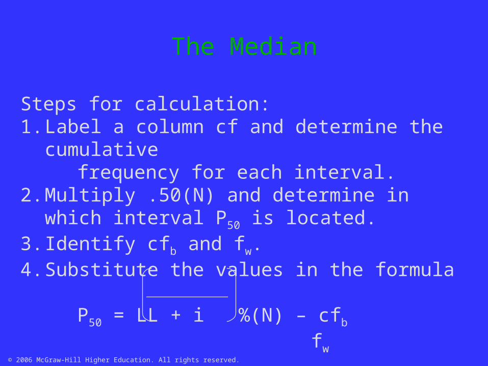
The Median

Steps for calculation:1. Label a column cf and determine the cumulative frequency for each interval.2. Multiply .50(N) and determine in which interval P50 is

located.3. Identify cfb and fw.4. Substitute the values in the formula

P50 = LL + i %(N) – cfb

fw


The Median

The calculation of the median from the distribution in table 2.7 is.50(75) = 37.5

P50 = 71.5 + 3 37.5 – 34 10

= 71.5 + 3 3.5 10 P50 =71.5 + 3(.35) = 72.55


Measures of Variability

Calculation of the range was described previously.

Quartile deviation and standard deviation will be coverednow.


The Quartile Deviation

The calculation of Q from the distribution in table 2.7 isQ3 Q1

.75(75) = 56.25 .25(75) = 18.75

Q3 = 80.5 + 3 56.25 – 56 Q1 = 62.5 + 3 18.75 – 16 7 6

= 80.5 + 3 .25 = 62.5 + 3 2.75 7 6

= 80.5 + .11 = 62.5 + 1.37Q3 = 80.61 Q1 = 63.87


The Quartile Deviation

Q = Q3 – Q1

2

= 80.61 – 63.87 2

= 16.74 2Q = 8.37


The Standard Deviation

New symbolfd2 = sum of d x fd

Steps for calculation:1. Label a column fd2 and determine fd2 for each interval.2. Calculate fd2.3. Substitute the values in the formula

s = i fd2 – fd 2

N N


The Standard Deviation

The calculation of s in the distribution in table 2.7 is

s = 3 973 - - 21 2

75 75

= 3 12.9733 – (.28)2

= 3 12.9733 - .0784

= 3 12.8949 s = 3 (3.59) = 10.77


Graphs

1. Enable individuals to interpret data without reading raw data or tables.2. Different types of graphs are used. Examples - histogram (column), frequency polygon (line), pie chart, area, scatter, and pyramid3. Standard guidelines should be used when constructing graphs.

See figures 2.7 and 2.8.


Standard Scores

Provide method for comparing unlike scores; can obtain an average score, or total score for unlike scores.

z-score - represents the number of standard deviations a raw score deviated from the mean

FORMULA

z = X - X s


z = X - X s

z = 88 - 72.2 = 15.8 z = 54 - 72.2 = -18.2 10.8 10.8 10.8 10.8z = 1.46 z = -1.69

INTERPRETATION?

Table 2.7- Tennis Serve ScoresScores of 88 and 54; X = 72.2; s = 10.8

z-Scores


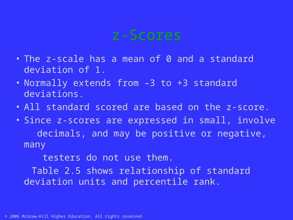
z-Scores

• The z-scale has a mean of 0 and a standard deviation of 1.

• Normally extends from –3 to +3 standard deviations.• All standard scored are based on the z-score.• Since z-scores are expressed in small, involve

decimals, and may be positive or negative, many

testers do not use them.

Table 2.5 shows relationship of standard deviation units and percentile rank.


T-ScoresT-scale• Has a mean of 50.• Has a standard deviation of 10.• May extend from 0 to 100.• Unlikely that any t-score will be beyond 20 or 80

(this range includes plus and minus 3 standard deviations).FormulaT-score = 50 + 10 (X - X) = 50 + 10z sFigure 2.9 shows the relationship of z-scores, T-scores, and the normal curve.


Figure 2.9 z-scores and T-scores plotted on normal curve.


T-Scores

Table 2.7 - Tennis Serve ScoresScores of 88 and 54; X = 72.2; s = 10.8

T88 = 50 + 10(1.46) T54 = 50 + 10 (-1.69) = 50 + 14.6 = 50 + (-16.9) = 64.6 = 65 = 33.1 = 33(T-scores are reported as whole numbers)


T-Scores

T-scores may be used in same way as z-scores, but usually preferred because:• Only positive whole numbers are reported.• Range from 0 to 100.

Sometime confusing because 60 or above is goodscore.


T-Scores

May convert raw scores in a distribution to T-scores

1. Number a column of T-scores from 20 to 80.2. Place the mean of the distribution of the scores opposite the T-score of 50.3. Divide the standard deviation of the distribution by ten. The standard deviation for the T-scale is 10, so each T-score from 0 to 100 is one-tenth of the standard deviation.


T-Scores

4. Add the value found in step 3 to the mean and each subsequent number until you reach the T-score of 80.5. Subtract the value found in step 3 from the mean and each decreasing number until you reach the number 20.6. Round off the scores to the nearest whole number.

*For some scores, lower scores are better (timed events).


Percentiles

• Are standard scores and may be used to compare scores of different measurements.

• Change at different rates (remember comparison of low and and high percentile scores with middle percentiles), so they should not be used to determine one score for several different tests.

• May prefer to use T-scale when converting raw scores to standard scores.

© 2006 McGraw-Hill Higher Education. All rights reserved. Chapter 2 Describing and Presenting a...

Documents

Transcript of © 2006 McGraw-Hill Higher Education. All rights reserved. Chapter 2 Describing and Presenting a...