Research Article Analyzing Axial Stress and Deformation...
10
Hindawi Publishing Corporation e Scientific World Journal Volume 2013, Article ID 565891, 9 pages http://dx.doi.org/10.1155/2013/565891 Research Article Analyzing Axial Stress and Deformation of Tubular for Steam Injection Process in Deviated Wells Based on the Varied (, ) Fields Yunqiang Liu, 1,2 Jiuping Xu, 1 Shize Wang, 3 and Bin Qi 3 1 Uncertainty Decision-Making Laboratory, Sichuan University, Chengdu 610064, China 2 College of Economics & Management, Sichuan Agricultural University, Chengdu 611130, China 3 Research School of Engineering Technology, e Southwest Petroleum and Gas Corp, China Petroleum and Chemical Corp, Deyang 618000, China Correspondence should be addressed to Jiuping Xu; [email protected] Received 13 May 2013; Accepted 2 August 2013 Academic Editors: G. Carbone, S. Park, S. Torii, and Q. Yang Copyright © 2013 Yunqiang Liu et al. is is an open access article distributed under the Creative Commons Attribution License, which permits unrestricted use, distribution, and reproduction in any medium, provided the original work is properly cited. e axial stress and deformation of high temperature high pressure deviated gas wells are studied. A new model is multiple nonlinear equation systems by comprehensive consideration of axial load of tubular string, internal and external fluid pressure, normal pressure between the tubular and well wall, and friction and viscous friction of fluid flowing. e varied temperature and pressure fields were researched by the coupled differential equations concerning mass, momentum, and energy equations instead of traditional methods. e axial load, the normal pressure, the friction, and four deformation lengths of tubular string are got ten by means of the dimensionless iterative interpolation algorithm. e basic data of the X Well, 1300 meters deep, are used for case history calculations. e results and some useful conclusions can provide technical reliability in the process of designing well testing in oil or gas wells. 1. Introduction e deviated wells had been wildly applicable for petroleum and natural gas industry. Deviated wells have their distinctive characteristics which are distinguished from that of other wells. (1) High temperature high pressure: the temperature distribution and pressure on the tubing are significantly different when outputs are varied (flow velocity) but neither has a simple linear relationship, because the fluid density is not constant. (2) Deep well: the sensibility of force and deformation influencing by the factors, such as the temper- ature, pressure, density of fluid, viscous friction and fluid velocity, and so forth, will become high with the increase of tubing length. e completion test of a deep well is a new problem. In the research of applied basic theory for deep well testing, tubular string mechanical analysis is very complex, but fluid temperature and tubing pressure affect the force of the tubular string heavily. Temperature, pressure, liquid density, and fluid velocity within tubing may change with of the hole depth, time, and operations, so that the axial force changes constantly. A large compression load at low end can induce the tubing plastic deformation and make the packer damaged. A large tension load at the top end may unpack the packer or cause the tubing to break. If the tubing failed, the whole borehole can hardly maintain its integrity and safety [1]. erefore, it is very important for deviated wells to predict the axial forces for the safety. Hammerlindl [2] had made a great contribution about tubular mechanics. He had put forth the four effects between the packer forces and length change of tubing: temperature effect, ballooning effect, axial load effect, and the helical buckling effect. ere is a large amount of papers to research the effect of buckling behavior. erefore it is considered that inflexion is caused on its axial force under certain conditions, by which colliding on parts of the drill string with well bore is induced. When buckled of tubular beyond wellhole’s control, the buckling configuration which will be transformed at the state of stabilization, sinusoidal buckling and helical buckling
Transcript of Research Article Analyzing Axial Stress and Deformation...
Hindawi Publishing CorporationThe Scientific World JournalVolume 2013 Article ID 565891 9 pageshttpdxdoiorg1011552013565891
Research ArticleAnalyzing Axial Stress and Deformation ofTubular for Steam Injection Process inDeviated Wells Based on the Varied (119879 119875) Fields
Yunqiang Liu12 Jiuping Xu1 Shize Wang3 and Bin Qi3
1 Uncertainty Decision-Making Laboratory Sichuan University Chengdu 610064 China2 College of Economics amp Management Sichuan Agricultural University Chengdu 611130 China3 Research School of Engineering Technology The Southwest Petroleum and Gas Corp China Petroleum and Chemical CorpDeyang 618000 China
Correspondence should be addressed to Jiuping Xu xujiupingscueducn
Received 13 May 2013 Accepted 2 August 2013
Academic Editors G Carbone S Park S Torii and Q Yang
Copyright copy 2013 Yunqiang Liu et al This is an open access article distributed under the Creative Commons Attribution Licensewhich permits unrestricted use distribution and reproduction in any medium provided the original work is properly cited
The axial stress and deformation of high temperature high pressure deviated gas wells are studied A new model is multiplenonlinear equation systems by comprehensive consideration of axial load of tubular string internal and external fluid pressurenormal pressure between the tubular and well wall and friction and viscous friction of fluid flowing The varied temperature andpressure fields were researched by the coupled differential equations concerning mass momentum and energy equations insteadof traditional methods The axial load the normal pressure the friction and four deformation lengths of tubular string are gotten by means of the dimensionless iterative interpolation algorithm The basic data of the X Well 1300 meters deep are used forcase history calculations The results and some useful conclusions can provide technical reliability in the process of designing welltesting in oil or gas wells
1 Introduction
The deviated wells had been wildly applicable for petroleumand natural gas industry Deviated wells have their distinctivecharacteristics which are distinguished from that of otherwells (1) High temperature high pressure the temperaturedistribution and pressure on the tubing are significantlydifferent when outputs are varied (flow velocity) but neitherhas a simple linear relationship because the fluid densityis not constant (2) Deep well the sensibility of force anddeformation influencing by the factors such as the temper-ature pressure density of fluid viscous friction and fluidvelocity and so forth will become high with the increase oftubing length The completion test of a deep well is a newproblem In the research of applied basic theory for deep welltesting tubular string mechanical analysis is very complexbut fluid temperature and tubing pressure affect the forceof the tubular string heavily Temperature pressure liquiddensity and fluid velocity within tubing may change with of
the hole depth time and operations so that the axial forcechanges constantly A large compression load at low end caninduce the tubing plastic deformation and make the packerdamaged A large tension load at the top end may unpack thepacker or cause the tubing to break If the tubing failed thewhole borehole can hardly maintain its integrity and safety[1]Therefore it is very important for deviatedwells to predictthe axial forces for the safety
Hammerlindl [2] had made a great contribution abouttubular mechanics He had put forth the four effects betweenthe packer forces and length change of tubing temperatureeffect ballooning effect axial load effect and the helicalbuckling effect There is a large amount of papers to researchthe effect of buckling behaviorTherefore it is considered thatinflexion is caused on its axial force under certain conditionsby which colliding on parts of the drill string with well bore isinduced When buckled of tubular beyond wellholersquos controlthe buckling configuration which will be transformed at thestate of stabilization sinusoidal buckling and helical buckling
2 The Scientific World Journal
with the increase of loadThe problem of buckling of the tubewas first studied and put into practice by Lubinski et al [3]They had done the emulation experiment for the bucklingbehavior of tube in deviated wells and found the computeformula on critical buckling load of tube in deviated wellsPaslay and Bogy [4] found that the number of sinusoids inthe buckling mode increases with the length of the tubeThe buckling behavior by inner and outer fluid pressure oftubing was analyzed and the mathematical relation betweenpitch and axial pressures was deduced based on the principleof minimum potential energy (see Hammerlindl [2]) Themptotic solution for sinusoidal buckling of an extremely longtube has been analyzed by Dawson and Paslay [5] based on asinusoidal buckling mode of constant amplitude Numericalsolutions were also sought by Mitchell [6] using the basicmechanics equations His solutions confirm the thought thatunder a general loading the deformed shape of the tube is acombination of helices and sinusoids while helical deforma-tion occurs only under special values of the applied loadTheformula about tubing forces had been put however which istoo simple for shallowwells to accommodate the complicatedstates of deep wells Up to now many researches are centeredonwater injection tubular but not on steam injection Amongthem the values of temperature and pressure are consideredas constant or lineal functions which will cause large errorson tubular deformation computing [7]
In fact the tubular string deformation includes trans-verse deformation and longitudinal deformation Becausethe transverse length (its order of magnitude is 10minus3m) ismuch and much smaller than the longitudinal length (itsorder of magnitude is 103m) we mainly consider the axial(longitudinal) deformation for the tubular string deformationanalysis in the paper In the paper the force states oftubular in the process of steam injection are analyzed Thevaried (119879 119875) fields are considered to compute the values ofseveral deformations The axial load and four deformationlengths of tubular string are obtained by the dimensionlessiterative interpolation algorithmThe basic data of the XWell(deviated well) 1300 meters deep in China are used for casehistory calculations Some useful suggestions are drawn
This paper is organized as follows Section 2 gives asystem model about tubular mechanics and deformationAnd the varied (119879 119875) fields were presented by model con-cerning mass momentum and energy balance Section 3gives the parameters initial condition and algorithm forsolving model In Section 4 we give an example from adeviated well at 1300 meters of depth in China and the resultanalysis are made Section 5 gives a conclusion
2 Model Building
21 Basic Assumption Before analyzing the force on themicroelement some assumptions are introduced as follows
(1) the curvature of the hole of the considered modularsection is constant
Pi
P0
D
d
o
r
z
Tube
Casing
Packer
Packerfluid
Figure 1 The physical figure of forces analysis on tube
(2) on the upper side or underside of the section whichis point of contact of the pipe and tube wall thecurvature is the same with the hole curvature
(3) the radius of steam injection string in contrast tocurvature of borehole is insignificant
(4) the string is at the state of linear elastic relationship
22 Forces Analysis of Tubular String The forces of tubularstring are shown in Figure 1 Consider the flow systemdepicted in Figure 1 a constant cross-sectional flow area 119860inner diameter 119889 outer diameter 119863 material density 120588
1
packer fluid density 120588
2
and a total length 119885 Through thistubing gas flows from the bottom to the top with a mass flowrate 119882 The distance coordinate in the flow direction alongthe tubing is denoted by 119911 The cylindrical coordinate system119903120579119911 origin of which is in wellhead and 119885 axis is down as theborehole axis is used
As shown fromFigure 1 the tubular string ismainly actedupon by the following forces at the process of steam injection
(1) Initial Axial Force The initial axial force of tubularshould include the deadweight buoyant weight andinitial pull force
(2) Thermal Stress On the process of steam injection thetemperature stress will act at the tubular with variedtemperature
(3) Axial Force by the Varied Internal and External Pres-sure Thanks to the varied pressure with internal andexternal pressure the tubular will be acted by thebending force piston force and other axial forces
(4) Friction Drag by Steam Injection On the process ofsteam injection the flow in tubular will produceviscous flow which will cause the friction drag
The Scientific World Journal 3
23 The Axial Load and Axial Stress of the Tubular
231 Initial Axial Load and Initial Axial Stress of SteamInjection Tubular
Initial Axial Load The section to which the distance from thewellhead is 119911(119898) was considered The axial static load by thedeadweight of tubular is as follows
119873119902119911
= int
119871
119911
119902 cos120572119889119911 =120587
41205881
119892 (1198632
minus 1198892
)int
119871
119911
cos120572119889119911 (1)
where 119873119902119911
is the deadweight of tubular 119902 is the average unitlength weight of tubing 119871 is the length of tubular 120588
1
is thedensity of tubular and 120572 is the inclination angle
The axial static load by the buoyant weight is as follows
119873119887119911
= minus1205882
1198921198602
int
119871
119911
cos120572119889119911 = minus1205882
119892119911120587(119863
2)
2
int
119871
119911
cos120572119889119911
(2)
where 119873119887119911
is the buoyant weight of tubular 1205882
is the densityof packer fluid
The axial load by the steam injection pressure
119873119901119911
=1198751199111
1205871198892
119911
4 (3)
where 1198751199111
represents the inner pressure at this sectionTherefore summing (1) (2) and (3) the axial forces in
the section are obtained as follows
119865119911
= 119873119902119911
+ 119873119887119911
+ 119873119901119911
(4)
Initial Axial Stress The axial stress can be derived from thefollowing equation
120590119911119894
=4119865119911
120587 (1198632
minus 1198892
) (5)
232 Axial Thermal Stress of Steam Injection Tubular In theprocess of steam injection the temperature of tubular willchange with time and depth which will make the tubulardeform as follows
120590119911119905
= 119864120573 (1198791199111
minus 1198791199110
) = 119864120573Δ119879 (6)
where 119864 represents the steel elastic modulus of tubular 120573 isthe warm balloon coefficient of the tubular string and Δ119879 isthe temperature change with before and after steam injection
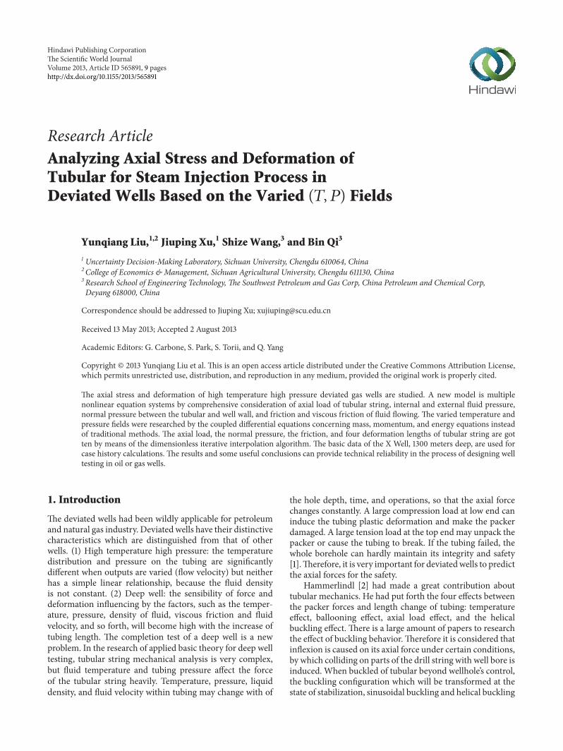
233 Axial Stress of Steam Injection Tubular by the Changewith Pressure The effect acting the tubular with pressurechange which is called ballooning effect normally
Ballooning Stress Analysis The ballooning effect will beproduced from pressure acted in inner and outer of the tubeGenerally there are two kinds of tubular in oil wells One isthe tubulars whose outer diameter is 889mm inner diameter
Pz1
Pz2D
d
Figure 2 The radial and tangential stresses figure of tube
is 76mm and thickness of tubes is 65mm (120575(1198892) =
171 gt 5) the other is the tubular whose outer diameter is1143mm inner diameter is 1005mm and thickness of tubesis 69mm (120575(1198892) = 137 gt 5) Neither is the thin-wallproblemTherefore it should be solved by Lamersquos formula [8]
The radial and tangential stresses in the thick-wall cylin-der can be shown as Figure 2 The two can be calculated asfollows
120590119903119911
=1198892
1198751199111
minus 1198632
1198751199110
1198632
minus 1198892
minus(1198751199111
minus 1198751199110
)1198632
1198892
(1198632
minus 1198892
) 41199032
120590120579119911
=1198892
1198751199111
minus 1198632
1198751199110
1198632
minus 1198892
+(1198751199111
minus 1198751199110
)1198632
1198892
(1198632
minus 1198892
) 41199032
(7)
where 119903 is radial stress 120579 is tangential stress 119903 (119889 le 119903 le 119863) isradial coordinate 119875
1199111
is tube internal pressure at 119911 point and1198751199110
is tube external pressure at 119911 point
234 Axial Stress of Steam Injection Tubular by the FrictionLoss In fact the flow in the tubular should be multiflow Onthe process of steam injection the flow will be run and it willgive rise to friction effect to cause axial stress In our paperwe consider the flow gas-liquid mix flow and the liquid headloss is gotten by the Darcy-Weisbach formula [9] as follows
ℎ119891
=120582 (119885 minus 119911) ]2
119898
2119892119889 (8)
where ℎ119891
means heat loss of liquid flow 120582 is frictional headlosses coefficients and ]
119898
is the velocity of liquid flowThe friction drag in tubular is 119873
119891119911
= ℎ119891
120588119898
1198921205871198892 (120588119898
isdensity of liquid flow) The axial stress by fiction drag can beobtained as follows
120590119911119891
=
4119873119891119911
120587 (1198632
minus 1198892
) (9)
24 Analysis of Axial Deformation Based on the studiesand analyses mentioned above the axial deformation on thetubular is made up of the following parts
4 The Scientific World Journal
241TheAxial Deformation by the Axial Static Stress For themicroelement of the tubular 119889119911 the unit deformation by thestatic stress can be computed by generalized Hooke law
1205761
=1
119864[120590119911119894
minus 120583 (120590119903119911
+ 120590120579119911
)] (10)
where 120583 represents Poissonrsquos ratiosThe axial deformation at an element can be obtained
through integrating on the length of the element as follows
Δ1198711119894
= int
119885119894
119885119894minus1
1
119864[120590119911119894
minus 120583 (120590119903119911
+ 120590120579119911
)] 119889119911 (11)
Therefore the total axial deformation by the static stresscan be gotten accumulating each element as follows
Δ1198711
=
119873
sum
119894=1
Δ1198711119894
(12)
242The Axial Deformation with Temperature Changed Forthe microelement of the tubular 119889119911 the unit deformation bythe temperature change is as follows
Δ1198712119894
= int
119885119894
119885119894minus1
120590119911119905
119864119889119911 = 120573Δ119879
119894
Δ119871119894
(13)
The same principle is that the total axial deformation bythe varied temperature fields can be gotten accumulating eachelement as follows
Δ1198712
=
119873
sum
119894=1
Δ1198712119894
(14)
243 The Axial Deformation with the Friction Drag For themicroelement of the tubular 119889119911 the unit deformation by thefriction force is as follows
Δ1198713
= int
119885
0
120590119911119891
119864119889119911 =
120582120588119898
]2119898
1198891198852
119864 (1198632
minus 1198892
) (15)
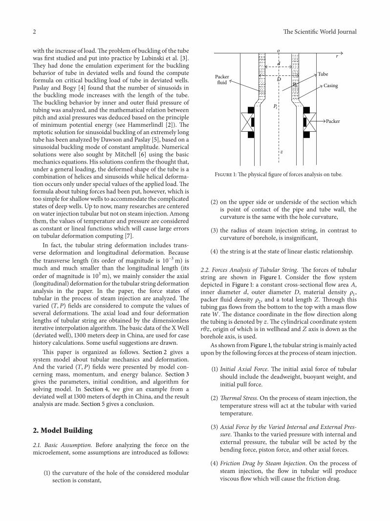
244TheAxial Deformationwith the Tubular String BucklingResearchers in general call the buckling a bending effect Thetubular is freely suspended in the absence of fluid inside asshown in Figure 3(a) Because the force 119865 applied at the endof the tubular which is large enough the tubular will buckleas shown in Figure 3(b)
Lubinski et al [3] had done many researches on thephenomenon From theirworkwe can get the buckling effectDefine the virtual axial force of tubing as follows
119865119891
= 119860119901
(1198751
minus 1198750
) (16)
where 1198751
is the pressure inside the tubular at the packerlength 119875
0
is the pressure outside the tubular at the packerlength and 119860
119901
is the area corresponding to packer boreBy (16) whether the tubular will buckle or not can be
judged The string will buckle if 119865119891
is positive or remain
(a)
F
Neutral point
(b)
Figure 3 Buckling of tubular
straight if 119865119891
is negative or zero The axial deformation of thetubular string buckling is
Δ1198714119894
= minus
1199032
1198602
119901
(Δ1198751119894
minus Δ1198750119894
)2
8119864119868119882
(17)
where 119903means tubing-to-casing radial clearance 119868 ismomentof inertia of tubing cross-section with respect to its diameter(119868 = 120587(119863
4
minus 1198894
)64) Δ denotes change with before and afterinjection and119882 is the unit weight of tubing as
Δ1198714
=
119873
sum
119894=1
Δ1198714119894
(18)
In addition the position of the neutral point is needed Thelength (119899) from the packer to the point can be computed asfollows
119899 =
119865119891
119882 (19)
Generally the neutral point should be in tubular (119899 le 119885)However at the multipackers it will occur that the neutralpoint is outside the tubing between dual packers In thispaper we leave the latter phenomenon
To sum up the whole deformation length can be repre-sented as follows
Δ119871 = Δ1198711
+ Δ1198712
+ Δ1198713
+ Δ1198714
(20)
25 The Analysis of the Varied (119879 119875) Fields In the courseof dryness modeling we can find that the numerical valuesof deformation ((10) (13) and (17)) were affected by thetemperature and pressure In fact the two parameters variedaccording to the depth and time changing So the varied(119879 119875) fields need to be researched Under the China Sinopec
The Scientific World Journal 5
Group Hi-Tech Project ldquoStress analysis and optimum designof well completionrdquo in 2009 [6] undertaken by SichuanUniversity at early time The varied (119879 119875) fields had beendeduced strictly based on the mass momentum and energybalance The proof details can be shown in Xu et al [11] Thevaried (119879 119875) fields is
119889119875
119889119911=
minus (120591119894
119860) + 120588119898
119892 cos 120579 + (119898119860) 119877 (119889119909119889119911)
1 minus (119898119860) 119878
119889119879
119889119911= minus
]119898
119862119875119892
(119877119889119909
119889119911minus 119878
119889119875
119889119911) minus
119892 cos 120579119862119875119892
minus120587119891119903119905119894
120588119898
]3119898
4119862119875119892
+119886 (119879 minus 119879
119890
)
119862119875119892
119875 (1199110
) = 1198750
119879 (1199110
) = 1198790
119889119909 (1199110
) = 1198891199090
119909 (1199110
) = 1199110
(21)
3 Numerical Implementation
31 Calculation of Some Parameters In this section we willgive the calculating method of some parameters
(1) Each pointrsquos inclination
120572119895
= 120572119895minus1
+
(120572119896
minus 120572119896minus1
) Δ119904119895
Δ119904119896
(22)
where 119895 represents segment point of calculation Δ119904119896
represents measurement depth of inclination angle120572119896
and 120572119896minus1
Δ119904119895
is the step length of calculationTransient heat transfer function [12]
119891 (119905119863
) =
1128radic119905119863
(1 minus 03radic119905119863
) 119905119863
le 15
(04063 + 05 ln 119905119863
) (1 +06
119905119863
) 119905119863
gt 15
(23)
(2) The density of wet steam Since the flow of the watervapor in is the gas-liquid two-phase flow there aremany researches about this problem [13 14] In thepaper we adopt the M-B model to calculate theaverage density of the mixture
(3) The heat transfer coefficient 119880to from different posi-tions of the axis of the wellbore to the second surface
These resistances include the tubing wall possible insu-lation around the tubing annular space (possibly filled witha gas or liquid but is sometimes vacuum) casing wall andcementing behind the casing as follows
1
119880119905119900
= 119903119905119894
1
120582insln(
119903119888119894
119903119905119900
) +1
ℎ119888
+ ℎ119903
+ 119903119905119894
1
120582cemln(
119903cem119903119888119900
) (24)
120582ins and 120582cem are the heat conductivity of the heat insulatingmaterial and the cement sheath respectively ℎ
119888
and ℎ119903
are thecoefficients of the convection heat transfer and the radiationheat transfer
32 Initial Condition In order to solve model some definiteconditions and initial conditions should be addedThe initialconditions comprise the distribution of the pressure andtemperature at the well top In this paper we adopt thevalue at the initial time by actual measurement Before steaminjected the temperature of tubular just is initial temperatureof formation (119879
119911
= 1198790
+ 120574119911 cos120572 120574 is geothermal gradient)At the same time the pressure of inner tubular is assumed tobe equal to the outer tubular before steam injected
33 Steps of Algorithm To simplify the calculation wedivided the wells into several short segments of the samelength The length of a segment varies depending on varia-tions in wall thickness hole diameter fluid density inside andoutside the pipe and wells geometry The model begins withthe calculation at one particular position in the wells the topof the pipe
Step 1 Set step length of depth In addition we denotethe relatively tolerant error by 120576 The smaller ℎ 120576 is themore accurate the results are However it will lead to rapidincreasing calculating time In our paper we set ℎ = 1 (m)and 120576 = 5
Step 2 Give the initial conditions
Step 3 Compute each pointrsquos inclination
Step 4 Compute the parameters under the initial conditionsor the last depth variables
Step 5 Let 119879 = 119879119896
then we can get the 119879119890
by solving thefollowing equation
120597119879119890
120597119905119863
= (1205972
119879119890
1205971199032
119863
+1
119903119863
120597119879119890
120597119903119863
)
119879119890
1003816100381610038161003816119905119863=0= 1198790
+ 120574119911 cos 120579
120597119879119890
120597119903119863
10038161003816100381610038161003816100381610038161003816119903119863=1
= minus1
2120587120582119891
119889119902
119889119911
120597119879119890
120597119903119863
10038161003816100381610038161003816100381610038161003816119903119863rarrinfin
= 0
(25)
Let 119879119895119890119894
be the temperature at the injection time 119895 andradial 119894 at the depth 119911 We apply the finite different methodto discretize the equations as follows
119879119894+1
119890119895
minus 119879119894
119890119895
120593=
119879119894+1
119890119895+1
minus 2119879119895
119890119895+1
+ 119879119894minus1
119890119895+1
1205852
minus
119879119894+1
119890119895+1
minus 119879119894+1
119890119895
119903119863
120593 (26)
where 120593 is the interval of time and 120585 is the interval of radialrespectively It can be transformed into the standard form asfollows
minus(120593 +120593120585
119903119863
)119879119894+1
119890119895+1
+ (2120593 +120593120585
119903119863
)119879119894+1
119890119895
minus 120593119879119894+1
119890119895minus1
= 1205852
119879119894
119890119895
(27)
6 The Scientific World Journal
Table 1 Parameters of pipes
Diameter (m) Thickness (m) Weight (Kg) Expansion Elastic (Gpa) Poissonrsquos ratios Using length (m)00889 001295 2379 00000115 215 03 27000889 000953 1828 00000115 215 03 12000889 000734 1504 00000115 215 03 62000889 000645 1358 00000115 215 03 290
Table 2 Well parameters
Measured (m) Internal (m) External (m)3367 015478 017784226 01525 0177813000 010862 0127
Table 3 Parameters of azimuth inclination and vertical depth
Number Measured(m)
Inclination(∘)
Azimuth(∘)
Vertical depth(m)
1 135 263 24101 134722 278 123 23786 277913 364 143 21386 363824 393 217 2638 392535 422 185 4456 421286 450 082 19112 449627 486 293 26907 485478 514 103 29755 513839 543 358 32451 5417410 571 298 30305 5704311 600 203 20474 5994212 628 234 16433 6272813 660 185 19528 6595614 723 314 21484 7217015 782 098 21648 7813016 830 215 22931 8291217 860 267 24403 8597118 908 485 26662 9040819 928 672 25878 9214220 972 203 23688 9717121 1025 478 23927 10212522 1058 401 24459 10555823 1089 498 2282 10841724 1132 375 23388 11292825 1174 563 23514 11688726 1204 423 23438 12009927 1235 387 23499 12320828 1268 497 23257 12634529 1300 884 23328 128496
Then the different method is used to discretize theboundary condition For 119903
119863
= 1 we have
119879119890119894+1
1198902
minus (1 +119886120585
2120587120582119891
)119879119894+1
1198901
=119886119879119896
2120587120582119891
(28)
For 119903119863
= 119873 we have
119879119894+1
119890119899
minus 119879119894+1
119890119899minus1
= 0 (29)We can compute the symbolic solution of the temperature 119879
119890
of the stratum In this stepwewill get the discrete distributionof 119879119890
as the following matrix
[[[[[[[[[[[[
[
1198791
1198901
1198792
1198901
sdot sdot sdot T1198941198901
sdot sdot sdot
1198791
1198902
1198792
1198902
sdot sdot sdot 119879119894
1198902
sdot sdot sdot
sdot sdot sdot
1198791
119890119895
1198792
119890119895
sdot sdot sdot 119879119894
119890119895
sdot sdot sdot
sdot sdot sdot
1198791
119890119899
1198792
119890119899
sdot sdot sdot 119879119894
119890119899
sdot sdot sdot
]]]]]]]]]]]]
]
(30)
where 119894 represents the injection time and 119895 represents theradial
Step 6 Let the right parts of the coupled differential equa-tions be functions 119865
119896
where (119896 = 1 2) Then we can obtain asystem of coupled functions as follows
1198651
=minus (120591119894
119860) + 120588119898
119892 cos 120579 + (119898119860) 119877 (119889119909119889119911)
1 minus (119898119860) 119878
1198652
= minus]119898
119862119875119892
(119877119889119909
119889119911minus 119878
119889119875
119889119911) minus
119892 cos 120579119862119875119892
minus120587119891119903119905119894
120588119898
]3119898
4119862119875119892
+119886 (119879 minus 119879
119890
)
119862119875119892
(31)
where 119879119890
at 119903119863
= 1
Step 7 Assume that 119875 119879 are 119910119896
(119896 = 1 2) respectively Thenwe can obtain some basic parameters as follows
119886119896
= 119865119894
(1199101
1199102
)
119887119896
= 119865119894
(1199101
+ℎ1198861
2 1199102
+ℎ1198862
2)
119888119896
= 119865119894
(1199101
+ℎ1198871
2 1199102
+ℎ1198872
2)
119889119896
= 119865119894
(1199101
+ ℎ1198881
1199102
+ ℎ1198882
)
(32)
The Scientific World Journal 7
Table 4 The results of the axial force and various kinds of deformation lengths
Number Depth(m)
Axial force(N)
Displacement bytemperaturechanged (m)
Displacement bypressure
changed (m)
Axial deformation(m)
Bucklingdeformation (m)
Total deformation(m)
1 1 8952448 0 0 0 0 02 100 8547248 01201 000986 0024 0 015443 200 8142155 02362 0019392 0052 0 030724 300 7737177 03483 0028598 0082 0 04595 400 737970 04564 0037476 0115 minus0006 060296 500 7068773 05606 0046028 0152 minus0006 075237 600 6757639 06607 0054254 0192 minus0006 090068 700 6446023 07569 0062153 0235 minus0006 10489 800 6134372 0849 0069725 0283 minus0007 1194610 900 5822721 09371 0076968 0335 minus0007 1342211 1000 5511072 10212 0083883 0391 minus0007 1489612 1100 5199423 11014 0090471 0452 minus0007 1636713 1200 4887775 11775 0096731 0517 minus0009 1782214 1300 4576128 12496 0102662 0584 minus001 19261
Step 8 Calculate the pressure and temperature at point(119895 + 1)
119910119895+1
119896
= 119910119895
119896
+ℎ (119886119896
+ 2119887119896
+ 2119888119896
+ 119889119896
)
6
119896 = 1 2 119895 = 1 2 119899
(33)
Step 9 Calculate the deformation Δ1198711119895
Δ1198712119895
and Δ1198714119895
byprevious equations
Step 10 Repeat the third step to the tenth step until tubularlength 119885 is calculated
Step 11 Calculate the deformationΔ1198713
and total deformationlength as follows
Δ119871 =
119873
sum
119895=1
Δ1198711119895
+
119873
sum
119895=1
Δ1198712119895
+ Δ1198713
+
119873
sum
119895=1
Δ1198714119895
(34)
4 Numerical Simulation
41 Parameters To demonstrate the application of our the-ory we study a pipe in X well which is in Sichuan ProvinceChina All the basic parameters are given as follows depthof the well is 1300m ground thermal conductivity parameteris 206 ground temperature is 16
∘C ground temperaturegradient is 00218 (∘Cm) roughness of the inner surface ofthe well is 0000015 and parameters of pipes inclined wellinclination azimuth and vertical depth are given in Tables 12 and 3
42 Main Results and Results Analysis After calculation weobtain a series of results of this well as Table 4 The influenceof outputs on the axial deformation of tubingwas investigatedas shown by Figure 4
25
2
15
1
05
0
Tota
l axi
al d
efor
mat
ion
(m)
Depth (m)1 1200800400
700000m3d500000m3d300000m3d
Figure 4 The total axial deformation under varied outputs
From the results as shown in Figure 4 and Table 4 someuseful analysis can be drawn
(1) The amount of steam injected and inject pressureaffected the stretching force with special severity
(2) The results were as follows the length of tubulardeformation was risen with increased injected pres-sure or injected velocity
(3) The length of tubular deformation increases with theincreasing of outputs but more slowly
(4) The thermal stress is the main factor influencing thetubular deformation Therefore the temperature ofsteam injected should not be too high
8 The Scientific World Journal
(5) The lifting prestressed cementing technology hasimportant meanings to reduce the deformation oftubular
(6) The creeping displacement of downhole stings willproduce an upward contractility which causes packerdepressed or lapsedTherefore the effective measuresshould be adopted to control the companding oftubular
5 Conclusion
In this paper a total tubular deformation model aboutdeviated wells was given A coupled-system model of differ-ential equations concerning pressure and temperature in hightemperature-high pressure steam injection wells according tomassmomentum and energy balances which can reduce theerror of axial stress and axial deformation was given insteadof the average value or simple linear relationship in traditionalresearch The basic data of the Well (high temperature andhigh pressure gas well) 1300m deep in Sichuan China wereused for case history calculations The results can providetechnical reliance for the process of designing well tests indeviated gas wells and dynamic analysis of production
Nomenclature
119889 Inner diameter (m)119889119911
Microelement of the tubular119892 Acceleration of gravity (ms2)ℎ Depth of top tubular located at the packer
(m)119905 Time of down stroke (s)119905119863
Dimensionless time (dimensionless)V119894
Velocity of fluid in tubing (ms)V119904
Velocity of down stroke (ms)119911 Distance coordinate in the flow direction
(m) along the tubing119860 Constant cross-sectional flow area (m2)119860119888
Effective area (m2)119860119901
Area corresponding to packer bore (m2)119862119869
The Joule-Thomson coefficient(dimensionless)
119862119875
Heat capacity of fluids (JKg sdotK)119863 Outer diameter (m)119864 Steel elastic modulus of tubular (Mpa)119865119894
Axial forces in the section (N)119865119911
Axial tensile strength (N)119865119891
Friction force (N)119865119888
Piston force for supporting packerrsquos pressure(N)
119865119904
Pumping force (N)119871 Length of tubular (m)119873119887119911
Buoyant weight of tubular (Kg)119873119902119911
Dead weight of tubular (Kg)1198750
Pressure outside the tubular (Mpa)1198751
Pressure inside the tubular at the packerlength (Mpa)
119875119894
Pressure in tubing (Mpa)119879119894
Temperature in tubing (∘C)119879119890
Initial temperature of formation (∘C)119882 Mass flow rate (Kgs)119885 Total length (m)1205881
Material density (Kgm3)1205882
Packer fluid density (Kgm3)120572 Inclination angle (∘)120573 Warm balloon coefficient of the tubular
string (dimensionless)120575 Drop of any parameter120590119911119905
Axial thermal stress (119873)120588119894
Density of fluid in the tubing (Kgm3)Δ1198713
The tubular string buckling axialdeformation (m)
Δ119871119905
Total axial deformation by variedtemperature fields (m)
Δ119871119887
Total axial deformation by the variedpressure fields (m)
Δ119875start Differential pressure at startup (Mpa)Δ119875119894119894
Change in tubing pressure at the 119894 length(Mpa)
Δ119875119900119894
Change in annulus pressure at the 119894 length(Mpa)
Δ119875119888
Differential pressure from top to bottom(Mpa)
Δ119879 Temperature change with before and afterwell shut-in (∘C)
Δ120588119894119894
Change in density of liquid in the tubing atthe 119894 length (Kgm3)
Δ120588119900119894
Change in density of liquid in the casing atthe 119894 length (Kgm3)
AcknowledgmentsThis research was supported by the Key Program of NSFC(Grant no 70831005) and the Key Project of China Petroleumand Chemical Corporation (Grant no GJ-73-0706)
References
[1] D-L Gao and B-K Gao ldquoA method for calculating tubingbehavior in HPHT wellsrdquo Journal of Petroleum Science andEngineering vol 41 no 1ndash3 pp 183ndash188 2004
[2] D J Hammerlindl ldquoMovement forces and stresses associatedwith combination tubing strings sealed in packersrdquo Journal ofPetroleum Technology vol 29 pp 195ndash208 1977
[3] A Lubinski W S Althouse and J L Logan ldquoHelical bucklingof tubular sealed in packersrdquo Journal of Petroleum Technologyvol 14 no 6 pp 655ndash670 1962
[4] P R Paslay and D B Bogy ldquoThe stability of a circular rodlaterally constrained to be in contact with an inclined circularcylinderrdquo Journal of Applied Mechanics vol 31 pp 605ndash6101964
[5] R Dawson and P R Paslay ldquoDrillpipe buckling in inclinedholesrdquo Journal of PetroleumTechnology vol 36 no 10 pp 1734ndash1738 1984
[6] R FMitchell ldquoEffects ofwell deviation onhelical bucklingrdquo SPEDrilling and Completion vol 12 no 1 pp 63ndash68 1997
The Scientific World Journal 9
[7] P Ding and X Z Yan ldquoForce analysis of high pressure waterinjection stringrdquo PetroleumDring Techiques vol 36 no 5 p 232005
[8] Z F Li ldquoCasing cementing with half warm-up for thermalrecovery wellsrdquo Journal of Petroleum Science and Engineeringvol 61 no 2ndash4 pp 94ndash98 2008
[9] A M Sun ldquoThe analysis and computing of water injectiontubularrdquo Drilling and Production Technology vol 26 no 3 pp55ndash57 2003 (Chinese)
[10] J P Xu ldquoStress analysis and optimum design of well comple-tionrdquo Technical Report of Sinopec GJ-73-0706 2009
[11] J P Xu Y Q Liu S Z Wang and B Qi ldquoNumerical modellingof steam quality in deviated wells with variable (T P) fieldsrdquoChemical Engineering Science vol 84 pp 242ndash254 2012
[12] A R Hasan and C S Kabir ldquoTwo-phase flow in vertical andinclined annulirdquo International Journal of Multiphase Flow vol18 no 2 pp 279ndash293 1992
[13] HD Beggs and J R Brill ldquoA study of two-phase flow in inclinedpipesrdquo Journal of Petroleum Technology vol 25 no 5 pp 607ndash617 1973 paper 4007-PA
[14] H Mukherjee and J P Brill ldquoPressure drop correlations forinclined two-phase flowrdquo Journal of Energy Resources Technol-ogy vol 107 no 4 pp 549ndash554 1985
International Journal of
AerospaceEngineeringHindawi Publishing Corporationhttpwwwhindawicom Volume 2014
RoboticsJournal of
Hindawi Publishing Corporationhttpwwwhindawicom Volume 2014
Hindawi Publishing Corporationhttpwwwhindawicom Volume 2014
Active and Passive Electronic Components
Control Scienceand Engineering
Journal of
Hindawi Publishing Corporationhttpwwwhindawicom Volume 2014
International Journal of
RotatingMachinery
Hindawi Publishing Corporationhttpwwwhindawicom Volume 2014
Hindawi Publishing Corporation httpwwwhindawicom
Journal ofEngineeringVolume 2014
Submit your manuscripts athttpwwwhindawicom
VLSI Design
Hindawi Publishing Corporationhttpwwwhindawicom Volume 2014
Hindawi Publishing Corporationhttpwwwhindawicom Volume 2014
Shock and Vibration
Hindawi Publishing Corporationhttpwwwhindawicom Volume 2014
Civil EngineeringAdvances in
Acoustics and VibrationAdvances in
Hindawi Publishing Corporationhttpwwwhindawicom Volume 2014
Hindawi Publishing Corporationhttpwwwhindawicom Volume 2014
Electrical and Computer Engineering
Journal of
Advances inOptoElectronics
Hindawi Publishing Corporation httpwwwhindawicom
Volume 2014
The Scientific World JournalHindawi Publishing Corporation httpwwwhindawicom Volume 2014
SensorsJournal of
Hindawi Publishing Corporationhttpwwwhindawicom Volume 2014
Modelling amp Simulation in EngineeringHindawi Publishing Corporation httpwwwhindawicom Volume 2014
Hindawi Publishing Corporationhttpwwwhindawicom Volume 2014
Chemical EngineeringInternational Journal of Antennas and
Propagation
International Journal of
Hindawi Publishing Corporationhttpwwwhindawicom Volume 2014
Hindawi Publishing Corporationhttpwwwhindawicom Volume 2014
Navigation and Observation
International Journal of
Hindawi Publishing Corporationhttpwwwhindawicom Volume 2014
DistributedSensor Networks
International Journal of
2 The Scientific World Journal
with the increase of loadThe problem of buckling of the tubewas first studied and put into practice by Lubinski et al [3]They had done the emulation experiment for the bucklingbehavior of tube in deviated wells and found the computeformula on critical buckling load of tube in deviated wellsPaslay and Bogy [4] found that the number of sinusoids inthe buckling mode increases with the length of the tubeThe buckling behavior by inner and outer fluid pressure oftubing was analyzed and the mathematical relation betweenpitch and axial pressures was deduced based on the principleof minimum potential energy (see Hammerlindl [2]) Themptotic solution for sinusoidal buckling of an extremely longtube has been analyzed by Dawson and Paslay [5] based on asinusoidal buckling mode of constant amplitude Numericalsolutions were also sought by Mitchell [6] using the basicmechanics equations His solutions confirm the thought thatunder a general loading the deformed shape of the tube is acombination of helices and sinusoids while helical deforma-tion occurs only under special values of the applied loadTheformula about tubing forces had been put however which istoo simple for shallowwells to accommodate the complicatedstates of deep wells Up to now many researches are centeredonwater injection tubular but not on steam injection Amongthem the values of temperature and pressure are consideredas constant or lineal functions which will cause large errorson tubular deformation computing [7]
In fact the tubular string deformation includes trans-verse deformation and longitudinal deformation Becausethe transverse length (its order of magnitude is 10minus3m) ismuch and much smaller than the longitudinal length (itsorder of magnitude is 103m) we mainly consider the axial(longitudinal) deformation for the tubular string deformationanalysis in the paper In the paper the force states oftubular in the process of steam injection are analyzed Thevaried (119879 119875) fields are considered to compute the values ofseveral deformations The axial load and four deformationlengths of tubular string are obtained by the dimensionlessiterative interpolation algorithmThe basic data of the XWell(deviated well) 1300 meters deep in China are used for casehistory calculations Some useful suggestions are drawn
This paper is organized as follows Section 2 gives asystem model about tubular mechanics and deformationAnd the varied (119879 119875) fields were presented by model con-cerning mass momentum and energy balance Section 3gives the parameters initial condition and algorithm forsolving model In Section 4 we give an example from adeviated well at 1300 meters of depth in China and the resultanalysis are made Section 5 gives a conclusion
2 Model Building
21 Basic Assumption Before analyzing the force on themicroelement some assumptions are introduced as follows
(1) the curvature of the hole of the considered modularsection is constant
Pi
P0
D
d
o
r
z
Tube
Casing
Packer
Packerfluid
Figure 1 The physical figure of forces analysis on tube
(2) on the upper side or underside of the section whichis point of contact of the pipe and tube wall thecurvature is the same with the hole curvature
(3) the radius of steam injection string in contrast tocurvature of borehole is insignificant
(4) the string is at the state of linear elastic relationship
22 Forces Analysis of Tubular String The forces of tubularstring are shown in Figure 1 Consider the flow systemdepicted in Figure 1 a constant cross-sectional flow area 119860inner diameter 119889 outer diameter 119863 material density 120588
1
packer fluid density 120588
2
and a total length 119885 Through thistubing gas flows from the bottom to the top with a mass flowrate 119882 The distance coordinate in the flow direction alongthe tubing is denoted by 119911 The cylindrical coordinate system119903120579119911 origin of which is in wellhead and 119885 axis is down as theborehole axis is used
As shown fromFigure 1 the tubular string ismainly actedupon by the following forces at the process of steam injection
(1) Initial Axial Force The initial axial force of tubularshould include the deadweight buoyant weight andinitial pull force
(2) Thermal Stress On the process of steam injection thetemperature stress will act at the tubular with variedtemperature
(3) Axial Force by the Varied Internal and External Pres-sure Thanks to the varied pressure with internal andexternal pressure the tubular will be acted by thebending force piston force and other axial forces
(4) Friction Drag by Steam Injection On the process ofsteam injection the flow in tubular will produceviscous flow which will cause the friction drag
The Scientific World Journal 3
23 The Axial Load and Axial Stress of the Tubular
231 Initial Axial Load and Initial Axial Stress of SteamInjection Tubular
Initial Axial Load The section to which the distance from thewellhead is 119911(119898) was considered The axial static load by thedeadweight of tubular is as follows
119873119902119911
= int
119871
119911
119902 cos120572119889119911 =120587
41205881
119892 (1198632
minus 1198892
)int
119871
119911
cos120572119889119911 (1)
where 119873119902119911
is the deadweight of tubular 119902 is the average unitlength weight of tubing 119871 is the length of tubular 120588
1
is thedensity of tubular and 120572 is the inclination angle
The axial static load by the buoyant weight is as follows
119873119887119911
= minus1205882
1198921198602
int
119871
119911
cos120572119889119911 = minus1205882
119892119911120587(119863
2)
2
int
119871
119911
cos120572119889119911
(2)
where 119873119887119911
is the buoyant weight of tubular 1205882
is the densityof packer fluid
The axial load by the steam injection pressure
119873119901119911
=1198751199111
1205871198892
119911
4 (3)
where 1198751199111
represents the inner pressure at this sectionTherefore summing (1) (2) and (3) the axial forces in
the section are obtained as follows
119865119911
= 119873119902119911
+ 119873119887119911
+ 119873119901119911
(4)
Initial Axial Stress The axial stress can be derived from thefollowing equation
120590119911119894
=4119865119911
120587 (1198632
minus 1198892
) (5)
232 Axial Thermal Stress of Steam Injection Tubular In theprocess of steam injection the temperature of tubular willchange with time and depth which will make the tubulardeform as follows
120590119911119905
= 119864120573 (1198791199111
minus 1198791199110
) = 119864120573Δ119879 (6)
where 119864 represents the steel elastic modulus of tubular 120573 isthe warm balloon coefficient of the tubular string and Δ119879 isthe temperature change with before and after steam injection
233 Axial Stress of Steam Injection Tubular by the Changewith Pressure The effect acting the tubular with pressurechange which is called ballooning effect normally
Ballooning Stress Analysis The ballooning effect will beproduced from pressure acted in inner and outer of the tubeGenerally there are two kinds of tubular in oil wells One isthe tubulars whose outer diameter is 889mm inner diameter
Pz1
Pz2D
d
Figure 2 The radial and tangential stresses figure of tube
is 76mm and thickness of tubes is 65mm (120575(1198892) =
171 gt 5) the other is the tubular whose outer diameter is1143mm inner diameter is 1005mm and thickness of tubesis 69mm (120575(1198892) = 137 gt 5) Neither is the thin-wallproblemTherefore it should be solved by Lamersquos formula [8]
The radial and tangential stresses in the thick-wall cylin-der can be shown as Figure 2 The two can be calculated asfollows
120590119903119911
=1198892
1198751199111
minus 1198632
1198751199110
1198632
minus 1198892
minus(1198751199111
minus 1198751199110
)1198632
1198892
(1198632
minus 1198892
) 41199032
120590120579119911
=1198892
1198751199111
minus 1198632
1198751199110
1198632
minus 1198892
+(1198751199111
minus 1198751199110
)1198632
1198892
(1198632
minus 1198892
) 41199032
(7)
where 119903 is radial stress 120579 is tangential stress 119903 (119889 le 119903 le 119863) isradial coordinate 119875
1199111
is tube internal pressure at 119911 point and1198751199110
is tube external pressure at 119911 point
234 Axial Stress of Steam Injection Tubular by the FrictionLoss In fact the flow in the tubular should be multiflow Onthe process of steam injection the flow will be run and it willgive rise to friction effect to cause axial stress In our paperwe consider the flow gas-liquid mix flow and the liquid headloss is gotten by the Darcy-Weisbach formula [9] as follows
ℎ119891
=120582 (119885 minus 119911) ]2
119898
2119892119889 (8)
where ℎ119891
means heat loss of liquid flow 120582 is frictional headlosses coefficients and ]
119898
is the velocity of liquid flowThe friction drag in tubular is 119873
119891119911
= ℎ119891
120588119898
1198921205871198892 (120588119898
isdensity of liquid flow) The axial stress by fiction drag can beobtained as follows
120590119911119891
=
4119873119891119911
120587 (1198632
minus 1198892
) (9)
24 Analysis of Axial Deformation Based on the studiesand analyses mentioned above the axial deformation on thetubular is made up of the following parts
4 The Scientific World Journal
241TheAxial Deformation by the Axial Static Stress For themicroelement of the tubular 119889119911 the unit deformation by thestatic stress can be computed by generalized Hooke law
1205761
=1
119864[120590119911119894
minus 120583 (120590119903119911
+ 120590120579119911
)] (10)
where 120583 represents Poissonrsquos ratiosThe axial deformation at an element can be obtained
through integrating on the length of the element as follows
Δ1198711119894
= int
119885119894
119885119894minus1
1
119864[120590119911119894
minus 120583 (120590119903119911
+ 120590120579119911
)] 119889119911 (11)
Therefore the total axial deformation by the static stresscan be gotten accumulating each element as follows
Δ1198711
=
119873
sum
119894=1
Δ1198711119894
(12)
242The Axial Deformation with Temperature Changed Forthe microelement of the tubular 119889119911 the unit deformation bythe temperature change is as follows
Δ1198712119894
= int
119885119894
119885119894minus1
120590119911119905
119864119889119911 = 120573Δ119879
119894
Δ119871119894
(13)
The same principle is that the total axial deformation bythe varied temperature fields can be gotten accumulating eachelement as follows
Δ1198712
=
119873
sum
119894=1
Δ1198712119894
(14)
243 The Axial Deformation with the Friction Drag For themicroelement of the tubular 119889119911 the unit deformation by thefriction force is as follows
Δ1198713
= int
119885
0
120590119911119891
119864119889119911 =
120582120588119898
]2119898
1198891198852
119864 (1198632
minus 1198892
) (15)
244TheAxial Deformationwith the Tubular String BucklingResearchers in general call the buckling a bending effect Thetubular is freely suspended in the absence of fluid inside asshown in Figure 3(a) Because the force 119865 applied at the endof the tubular which is large enough the tubular will buckleas shown in Figure 3(b)
Lubinski et al [3] had done many researches on thephenomenon From theirworkwe can get the buckling effectDefine the virtual axial force of tubing as follows
119865119891
= 119860119901
(1198751
minus 1198750
) (16)
where 1198751
is the pressure inside the tubular at the packerlength 119875
0
is the pressure outside the tubular at the packerlength and 119860
119901
is the area corresponding to packer boreBy (16) whether the tubular will buckle or not can be
judged The string will buckle if 119865119891
is positive or remain
(a)
F
Neutral point
(b)
Figure 3 Buckling of tubular
straight if 119865119891
is negative or zero The axial deformation of thetubular string buckling is
Δ1198714119894
= minus
1199032
1198602
119901
(Δ1198751119894
minus Δ1198750119894
)2
8119864119868119882
(17)
where 119903means tubing-to-casing radial clearance 119868 ismomentof inertia of tubing cross-section with respect to its diameter(119868 = 120587(119863
4
minus 1198894
)64) Δ denotes change with before and afterinjection and119882 is the unit weight of tubing as
Δ1198714
=
119873
sum
119894=1
Δ1198714119894
(18)
In addition the position of the neutral point is needed Thelength (119899) from the packer to the point can be computed asfollows
119899 =
119865119891
119882 (19)
Generally the neutral point should be in tubular (119899 le 119885)However at the multipackers it will occur that the neutralpoint is outside the tubing between dual packers In thispaper we leave the latter phenomenon
To sum up the whole deformation length can be repre-sented as follows
Δ119871 = Δ1198711
+ Δ1198712
+ Δ1198713
+ Δ1198714
(20)
25 The Analysis of the Varied (119879 119875) Fields In the courseof dryness modeling we can find that the numerical valuesof deformation ((10) (13) and (17)) were affected by thetemperature and pressure In fact the two parameters variedaccording to the depth and time changing So the varied(119879 119875) fields need to be researched Under the China Sinopec
The Scientific World Journal 5
Group Hi-Tech Project ldquoStress analysis and optimum designof well completionrdquo in 2009 [6] undertaken by SichuanUniversity at early time The varied (119879 119875) fields had beendeduced strictly based on the mass momentum and energybalance The proof details can be shown in Xu et al [11] Thevaried (119879 119875) fields is
119889119875
119889119911=
minus (120591119894
119860) + 120588119898
119892 cos 120579 + (119898119860) 119877 (119889119909119889119911)
1 minus (119898119860) 119878
119889119879
119889119911= minus
]119898
119862119875119892
(119877119889119909
119889119911minus 119878
119889119875
119889119911) minus
119892 cos 120579119862119875119892
minus120587119891119903119905119894
120588119898
]3119898
4119862119875119892
+119886 (119879 minus 119879
119890
)
119862119875119892
119875 (1199110
) = 1198750
119879 (1199110
) = 1198790
119889119909 (1199110
) = 1198891199090
119909 (1199110
) = 1199110
(21)
3 Numerical Implementation
31 Calculation of Some Parameters In this section we willgive the calculating method of some parameters
(1) Each pointrsquos inclination
120572119895
= 120572119895minus1
+
(120572119896
minus 120572119896minus1
) Δ119904119895
Δ119904119896
(22)
where 119895 represents segment point of calculation Δ119904119896
represents measurement depth of inclination angle120572119896
and 120572119896minus1
Δ119904119895
is the step length of calculationTransient heat transfer function [12]
119891 (119905119863
) =
1128radic119905119863
(1 minus 03radic119905119863
) 119905119863
le 15
(04063 + 05 ln 119905119863
) (1 +06
119905119863
) 119905119863
gt 15
(23)
(2) The density of wet steam Since the flow of the watervapor in is the gas-liquid two-phase flow there aremany researches about this problem [13 14] In thepaper we adopt the M-B model to calculate theaverage density of the mixture
(3) The heat transfer coefficient 119880to from different posi-tions of the axis of the wellbore to the second surface
These resistances include the tubing wall possible insu-lation around the tubing annular space (possibly filled witha gas or liquid but is sometimes vacuum) casing wall andcementing behind the casing as follows
1
119880119905119900
= 119903119905119894
1
120582insln(
119903119888119894
119903119905119900
) +1
ℎ119888
+ ℎ119903
+ 119903119905119894
1
120582cemln(
119903cem119903119888119900
) (24)
120582ins and 120582cem are the heat conductivity of the heat insulatingmaterial and the cement sheath respectively ℎ
119888
and ℎ119903
are thecoefficients of the convection heat transfer and the radiationheat transfer
32 Initial Condition In order to solve model some definiteconditions and initial conditions should be addedThe initialconditions comprise the distribution of the pressure andtemperature at the well top In this paper we adopt thevalue at the initial time by actual measurement Before steaminjected the temperature of tubular just is initial temperatureof formation (119879
119911
= 1198790
+ 120574119911 cos120572 120574 is geothermal gradient)At the same time the pressure of inner tubular is assumed tobe equal to the outer tubular before steam injected
33 Steps of Algorithm To simplify the calculation wedivided the wells into several short segments of the samelength The length of a segment varies depending on varia-tions in wall thickness hole diameter fluid density inside andoutside the pipe and wells geometry The model begins withthe calculation at one particular position in the wells the topof the pipe
Step 1 Set step length of depth In addition we denotethe relatively tolerant error by 120576 The smaller ℎ 120576 is themore accurate the results are However it will lead to rapidincreasing calculating time In our paper we set ℎ = 1 (m)and 120576 = 5
Step 2 Give the initial conditions
Step 3 Compute each pointrsquos inclination
Step 4 Compute the parameters under the initial conditionsor the last depth variables
Step 5 Let 119879 = 119879119896
then we can get the 119879119890
by solving thefollowing equation
120597119879119890
120597119905119863
= (1205972
119879119890
1205971199032
119863
+1
119903119863
120597119879119890
120597119903119863
)
119879119890
1003816100381610038161003816119905119863=0= 1198790
+ 120574119911 cos 120579
120597119879119890
120597119903119863
10038161003816100381610038161003816100381610038161003816119903119863=1
= minus1
2120587120582119891
119889119902
119889119911
120597119879119890
120597119903119863
10038161003816100381610038161003816100381610038161003816119903119863rarrinfin
= 0
(25)
Let 119879119895119890119894
be the temperature at the injection time 119895 andradial 119894 at the depth 119911 We apply the finite different methodto discretize the equations as follows
119879119894+1
119890119895
minus 119879119894
119890119895
120593=
119879119894+1
119890119895+1
minus 2119879119895
119890119895+1
+ 119879119894minus1
119890119895+1
1205852
minus
119879119894+1
119890119895+1
minus 119879119894+1
119890119895
119903119863
120593 (26)
where 120593 is the interval of time and 120585 is the interval of radialrespectively It can be transformed into the standard form asfollows
minus(120593 +120593120585
119903119863
)119879119894+1
119890119895+1
+ (2120593 +120593120585
119903119863
)119879119894+1
119890119895
minus 120593119879119894+1
119890119895minus1
= 1205852
119879119894
119890119895
(27)
6 The Scientific World Journal
Table 1 Parameters of pipes
Diameter (m) Thickness (m) Weight (Kg) Expansion Elastic (Gpa) Poissonrsquos ratios Using length (m)00889 001295 2379 00000115 215 03 27000889 000953 1828 00000115 215 03 12000889 000734 1504 00000115 215 03 62000889 000645 1358 00000115 215 03 290
Table 2 Well parameters
Measured (m) Internal (m) External (m)3367 015478 017784226 01525 0177813000 010862 0127
Table 3 Parameters of azimuth inclination and vertical depth
Number Measured(m)
Inclination(∘)
Azimuth(∘)
Vertical depth(m)
1 135 263 24101 134722 278 123 23786 277913 364 143 21386 363824 393 217 2638 392535 422 185 4456 421286 450 082 19112 449627 486 293 26907 485478 514 103 29755 513839 543 358 32451 5417410 571 298 30305 5704311 600 203 20474 5994212 628 234 16433 6272813 660 185 19528 6595614 723 314 21484 7217015 782 098 21648 7813016 830 215 22931 8291217 860 267 24403 8597118 908 485 26662 9040819 928 672 25878 9214220 972 203 23688 9717121 1025 478 23927 10212522 1058 401 24459 10555823 1089 498 2282 10841724 1132 375 23388 11292825 1174 563 23514 11688726 1204 423 23438 12009927 1235 387 23499 12320828 1268 497 23257 12634529 1300 884 23328 128496
Then the different method is used to discretize theboundary condition For 119903
119863
= 1 we have
119879119890119894+1
1198902
minus (1 +119886120585
2120587120582119891
)119879119894+1
1198901
=119886119879119896
2120587120582119891
(28)
For 119903119863
= 119873 we have
119879119894+1
119890119899
minus 119879119894+1
119890119899minus1
= 0 (29)We can compute the symbolic solution of the temperature 119879
119890
of the stratum In this stepwewill get the discrete distributionof 119879119890
as the following matrix
[[[[[[[[[[[[
[
1198791
1198901
1198792
1198901
sdot sdot sdot T1198941198901
sdot sdot sdot
1198791
1198902
1198792
1198902
sdot sdot sdot 119879119894
1198902
sdot sdot sdot
sdot sdot sdot
1198791
119890119895
1198792
119890119895
sdot sdot sdot 119879119894
119890119895
sdot sdot sdot
sdot sdot sdot
1198791
119890119899
1198792
119890119899
sdot sdot sdot 119879119894
119890119899
sdot sdot sdot
]]]]]]]]]]]]
]
(30)
where 119894 represents the injection time and 119895 represents theradial
Step 6 Let the right parts of the coupled differential equa-tions be functions 119865
119896
where (119896 = 1 2) Then we can obtain asystem of coupled functions as follows
1198651
=minus (120591119894
119860) + 120588119898
119892 cos 120579 + (119898119860) 119877 (119889119909119889119911)
1 minus (119898119860) 119878
1198652
= minus]119898
119862119875119892
(119877119889119909
119889119911minus 119878
119889119875
119889119911) minus
119892 cos 120579119862119875119892
minus120587119891119903119905119894
120588119898
]3119898
4119862119875119892
+119886 (119879 minus 119879
119890
)
119862119875119892
(31)
where 119879119890
at 119903119863
= 1
Step 7 Assume that 119875 119879 are 119910119896
(119896 = 1 2) respectively Thenwe can obtain some basic parameters as follows
119886119896
= 119865119894
(1199101
1199102
)
119887119896
= 119865119894
(1199101
+ℎ1198861
2 1199102
+ℎ1198862
2)
119888119896
= 119865119894
(1199101
+ℎ1198871
2 1199102
+ℎ1198872
2)
119889119896
= 119865119894
(1199101
+ ℎ1198881
1199102
+ ℎ1198882
)
(32)
The Scientific World Journal 7
Table 4 The results of the axial force and various kinds of deformation lengths
Number Depth(m)
Axial force(N)
Displacement bytemperaturechanged (m)
Displacement bypressure
changed (m)
Axial deformation(m)
Bucklingdeformation (m)
Total deformation(m)
1 1 8952448 0 0 0 0 02 100 8547248 01201 000986 0024 0 015443 200 8142155 02362 0019392 0052 0 030724 300 7737177 03483 0028598 0082 0 04595 400 737970 04564 0037476 0115 minus0006 060296 500 7068773 05606 0046028 0152 minus0006 075237 600 6757639 06607 0054254 0192 minus0006 090068 700 6446023 07569 0062153 0235 minus0006 10489 800 6134372 0849 0069725 0283 minus0007 1194610 900 5822721 09371 0076968 0335 minus0007 1342211 1000 5511072 10212 0083883 0391 minus0007 1489612 1100 5199423 11014 0090471 0452 minus0007 1636713 1200 4887775 11775 0096731 0517 minus0009 1782214 1300 4576128 12496 0102662 0584 minus001 19261
Step 8 Calculate the pressure and temperature at point(119895 + 1)
119910119895+1
119896
= 119910119895
119896
+ℎ (119886119896
+ 2119887119896
+ 2119888119896
+ 119889119896
)
6
119896 = 1 2 119895 = 1 2 119899
(33)
Step 9 Calculate the deformation Δ1198711119895
Δ1198712119895
and Δ1198714119895
byprevious equations
Step 10 Repeat the third step to the tenth step until tubularlength 119885 is calculated
Step 11 Calculate the deformationΔ1198713
and total deformationlength as follows
Δ119871 =
119873
sum
119895=1
Δ1198711119895
+
119873
sum
119895=1
Δ1198712119895
+ Δ1198713
+
119873
sum
119895=1
Δ1198714119895
(34)
4 Numerical Simulation
41 Parameters To demonstrate the application of our the-ory we study a pipe in X well which is in Sichuan ProvinceChina All the basic parameters are given as follows depthof the well is 1300m ground thermal conductivity parameteris 206 ground temperature is 16
∘C ground temperaturegradient is 00218 (∘Cm) roughness of the inner surface ofthe well is 0000015 and parameters of pipes inclined wellinclination azimuth and vertical depth are given in Tables 12 and 3
42 Main Results and Results Analysis After calculation weobtain a series of results of this well as Table 4 The influenceof outputs on the axial deformation of tubingwas investigatedas shown by Figure 4
25
2
15
1
05
0
Tota
l axi
al d
efor
mat
ion
(m)
Depth (m)1 1200800400
700000m3d500000m3d300000m3d
Figure 4 The total axial deformation under varied outputs
From the results as shown in Figure 4 and Table 4 someuseful analysis can be drawn
(1) The amount of steam injected and inject pressureaffected the stretching force with special severity
(2) The results were as follows the length of tubulardeformation was risen with increased injected pres-sure or injected velocity
(3) The length of tubular deformation increases with theincreasing of outputs but more slowly
(4) The thermal stress is the main factor influencing thetubular deformation Therefore the temperature ofsteam injected should not be too high
8 The Scientific World Journal
(5) The lifting prestressed cementing technology hasimportant meanings to reduce the deformation oftubular
(6) The creeping displacement of downhole stings willproduce an upward contractility which causes packerdepressed or lapsedTherefore the effective measuresshould be adopted to control the companding oftubular
5 Conclusion
In this paper a total tubular deformation model aboutdeviated wells was given A coupled-system model of differ-ential equations concerning pressure and temperature in hightemperature-high pressure steam injection wells according tomassmomentum and energy balances which can reduce theerror of axial stress and axial deformation was given insteadof the average value or simple linear relationship in traditionalresearch The basic data of the Well (high temperature andhigh pressure gas well) 1300m deep in Sichuan China wereused for case history calculations The results can providetechnical reliance for the process of designing well tests indeviated gas wells and dynamic analysis of production
Nomenclature
119889 Inner diameter (m)119889119911
Microelement of the tubular119892 Acceleration of gravity (ms2)ℎ Depth of top tubular located at the packer
(m)119905 Time of down stroke (s)119905119863
Dimensionless time (dimensionless)V119894
Velocity of fluid in tubing (ms)V119904
Velocity of down stroke (ms)119911 Distance coordinate in the flow direction
(m) along the tubing119860 Constant cross-sectional flow area (m2)119860119888
Effective area (m2)119860119901
Area corresponding to packer bore (m2)119862119869
The Joule-Thomson coefficient(dimensionless)
119862119875
Heat capacity of fluids (JKg sdotK)119863 Outer diameter (m)119864 Steel elastic modulus of tubular (Mpa)119865119894
Axial forces in the section (N)119865119911
Axial tensile strength (N)119865119891
Friction force (N)119865119888
Piston force for supporting packerrsquos pressure(N)
119865119904
Pumping force (N)119871 Length of tubular (m)119873119887119911
Buoyant weight of tubular (Kg)119873119902119911
Dead weight of tubular (Kg)1198750
Pressure outside the tubular (Mpa)1198751
Pressure inside the tubular at the packerlength (Mpa)
119875119894
Pressure in tubing (Mpa)119879119894
Temperature in tubing (∘C)119879119890
Initial temperature of formation (∘C)119882 Mass flow rate (Kgs)119885 Total length (m)1205881
Material density (Kgm3)1205882
Packer fluid density (Kgm3)120572 Inclination angle (∘)120573 Warm balloon coefficient of the tubular
string (dimensionless)120575 Drop of any parameter120590119911119905
Axial thermal stress (119873)120588119894
Density of fluid in the tubing (Kgm3)Δ1198713
The tubular string buckling axialdeformation (m)
Δ119871119905
Total axial deformation by variedtemperature fields (m)
Δ119871119887
Total axial deformation by the variedpressure fields (m)
Δ119875start Differential pressure at startup (Mpa)Δ119875119894119894
Change in tubing pressure at the 119894 length(Mpa)
Δ119875119900119894
Change in annulus pressure at the 119894 length(Mpa)
Δ119875119888
Differential pressure from top to bottom(Mpa)
Δ119879 Temperature change with before and afterwell shut-in (∘C)
Δ120588119894119894
Change in density of liquid in the tubing atthe 119894 length (Kgm3)
Δ120588119900119894
Change in density of liquid in the casing atthe 119894 length (Kgm3)
AcknowledgmentsThis research was supported by the Key Program of NSFC(Grant no 70831005) and the Key Project of China Petroleumand Chemical Corporation (Grant no GJ-73-0706)
References
[1] D-L Gao and B-K Gao ldquoA method for calculating tubingbehavior in HPHT wellsrdquo Journal of Petroleum Science andEngineering vol 41 no 1ndash3 pp 183ndash188 2004
[2] D J Hammerlindl ldquoMovement forces and stresses associatedwith combination tubing strings sealed in packersrdquo Journal ofPetroleum Technology vol 29 pp 195ndash208 1977
[3] A Lubinski W S Althouse and J L Logan ldquoHelical bucklingof tubular sealed in packersrdquo Journal of Petroleum Technologyvol 14 no 6 pp 655ndash670 1962
[4] P R Paslay and D B Bogy ldquoThe stability of a circular rodlaterally constrained to be in contact with an inclined circularcylinderrdquo Journal of Applied Mechanics vol 31 pp 605ndash6101964
[5] R Dawson and P R Paslay ldquoDrillpipe buckling in inclinedholesrdquo Journal of PetroleumTechnology vol 36 no 10 pp 1734ndash1738 1984
[6] R FMitchell ldquoEffects ofwell deviation onhelical bucklingrdquo SPEDrilling and Completion vol 12 no 1 pp 63ndash68 1997
The Scientific World Journal 9
[7] P Ding and X Z Yan ldquoForce analysis of high pressure waterinjection stringrdquo PetroleumDring Techiques vol 36 no 5 p 232005
[8] Z F Li ldquoCasing cementing with half warm-up for thermalrecovery wellsrdquo Journal of Petroleum Science and Engineeringvol 61 no 2ndash4 pp 94ndash98 2008
[9] A M Sun ldquoThe analysis and computing of water injectiontubularrdquo Drilling and Production Technology vol 26 no 3 pp55ndash57 2003 (Chinese)
[10] J P Xu ldquoStress analysis and optimum design of well comple-tionrdquo Technical Report of Sinopec GJ-73-0706 2009
[11] J P Xu Y Q Liu S Z Wang and B Qi ldquoNumerical modellingof steam quality in deviated wells with variable (T P) fieldsrdquoChemical Engineering Science vol 84 pp 242ndash254 2012
[12] A R Hasan and C S Kabir ldquoTwo-phase flow in vertical andinclined annulirdquo International Journal of Multiphase Flow vol18 no 2 pp 279ndash293 1992
[13] HD Beggs and J R Brill ldquoA study of two-phase flow in inclinedpipesrdquo Journal of Petroleum Technology vol 25 no 5 pp 607ndash617 1973 paper 4007-PA
[14] H Mukherjee and J P Brill ldquoPressure drop correlations forinclined two-phase flowrdquo Journal of Energy Resources Technol-ogy vol 107 no 4 pp 549ndash554 1985
International Journal of
AerospaceEngineeringHindawi Publishing Corporationhttpwwwhindawicom Volume 2014
RoboticsJournal of
Hindawi Publishing Corporationhttpwwwhindawicom Volume 2014
Hindawi Publishing Corporationhttpwwwhindawicom Volume 2014
Active and Passive Electronic Components
Control Scienceand Engineering
Journal of
Hindawi Publishing Corporationhttpwwwhindawicom Volume 2014
International Journal of
RotatingMachinery
Hindawi Publishing Corporationhttpwwwhindawicom Volume 2014
Hindawi Publishing Corporation httpwwwhindawicom
Journal ofEngineeringVolume 2014
Submit your manuscripts athttpwwwhindawicom
VLSI Design
Hindawi Publishing Corporationhttpwwwhindawicom Volume 2014
Hindawi Publishing Corporationhttpwwwhindawicom Volume 2014
Shock and Vibration
Hindawi Publishing Corporationhttpwwwhindawicom Volume 2014
Civil EngineeringAdvances in
Acoustics and VibrationAdvances in
Hindawi Publishing Corporationhttpwwwhindawicom Volume 2014
Hindawi Publishing Corporationhttpwwwhindawicom Volume 2014
Electrical and Computer Engineering
Journal of
Advances inOptoElectronics
Hindawi Publishing Corporation httpwwwhindawicom
Volume 2014
The Scientific World JournalHindawi Publishing Corporation httpwwwhindawicom Volume 2014
SensorsJournal of
Hindawi Publishing Corporationhttpwwwhindawicom Volume 2014
Modelling amp Simulation in EngineeringHindawi Publishing Corporation httpwwwhindawicom Volume 2014
Hindawi Publishing Corporationhttpwwwhindawicom Volume 2014
Chemical EngineeringInternational Journal of Antennas and
Propagation
International Journal of
Hindawi Publishing Corporationhttpwwwhindawicom Volume 2014
Hindawi Publishing Corporationhttpwwwhindawicom Volume 2014
Navigation and Observation
International Journal of
Hindawi Publishing Corporationhttpwwwhindawicom Volume 2014
DistributedSensor Networks
International Journal of
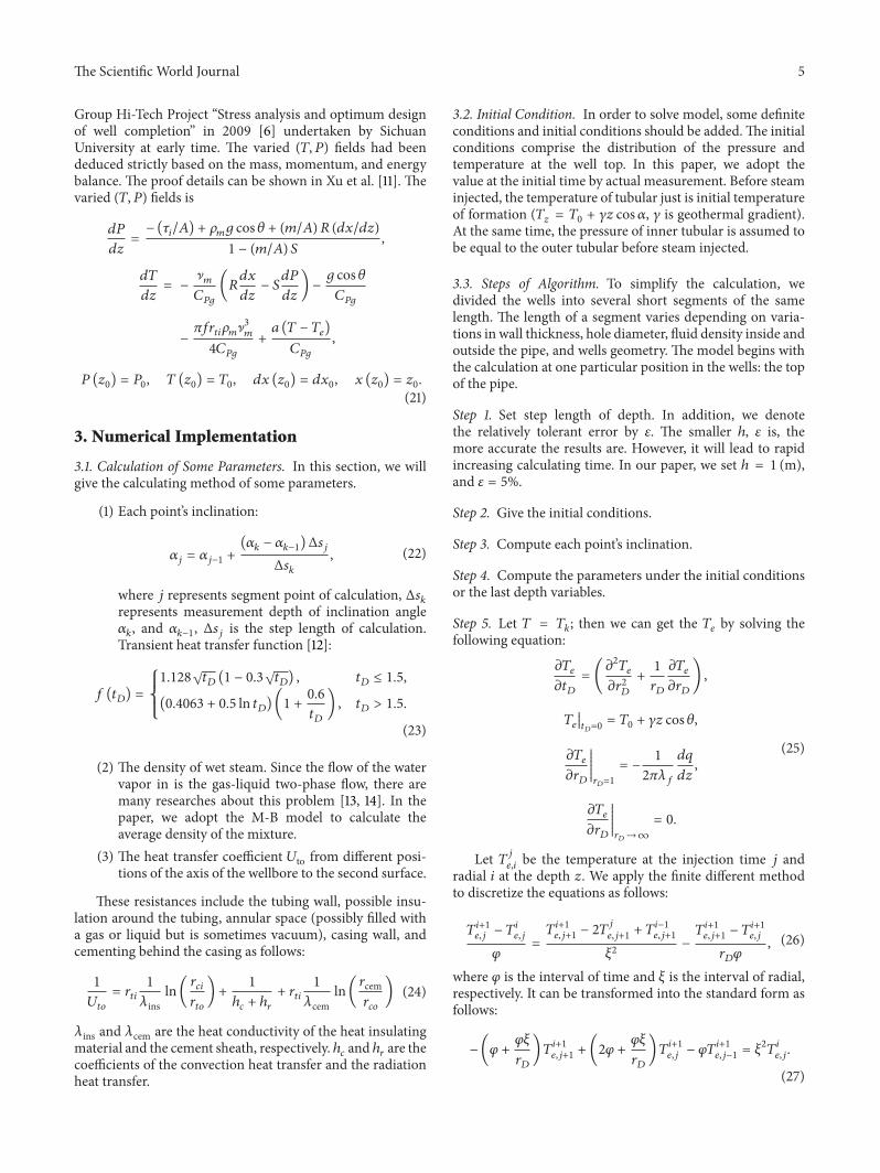

International Journal of
AerospaceEngineeringHindawi Publishing Corporationhttpwwwhindawicom Volume 2014
RoboticsJournal of
Hindawi Publishing Corporationhttpwwwhindawicom Volume 2014
Hindawi Publishing Corporationhttpwwwhindawicom Volume 2014
Active and Passive Electronic Components
Control Scienceand Engineering
Journal of
Hindawi Publishing Corporationhttpwwwhindawicom Volume 2014
International Journal of
RotatingMachinery
Hindawi Publishing Corporationhttpwwwhindawicom Volume 2014
Hindawi Publishing Corporation httpwwwhindawicom
Journal ofEngineeringVolume 2014
Submit your manuscripts athttpwwwhindawicom
VLSI Design
Hindawi Publishing Corporationhttpwwwhindawicom Volume 2014
Hindawi Publishing Corporationhttpwwwhindawicom Volume 2014
Shock and Vibration
Hindawi Publishing Corporationhttpwwwhindawicom Volume 2014
Civil EngineeringAdvances in
Acoustics and VibrationAdvances in
Hindawi Publishing Corporationhttpwwwhindawicom Volume 2014
Hindawi Publishing Corporationhttpwwwhindawicom Volume 2014
Electrical and Computer Engineering
Journal of
Advances inOptoElectronics
Hindawi Publishing Corporation httpwwwhindawicom
Volume 2014
The Scientific World JournalHindawi Publishing Corporation httpwwwhindawicom Volume 2014
SensorsJournal of
Hindawi Publishing Corporationhttpwwwhindawicom Volume 2014
Modelling amp Simulation in EngineeringHindawi Publishing Corporation httpwwwhindawicom Volume 2014
Hindawi Publishing Corporationhttpwwwhindawicom Volume 2014
Chemical EngineeringInternational Journal of Antennas and
Propagation
International Journal of
Hindawi Publishing Corporationhttpwwwhindawicom Volume 2014
Hindawi Publishing Corporationhttpwwwhindawicom Volume 2014
Navigation and Observation
International Journal of
Hindawi Publishing Corporationhttpwwwhindawicom Volume 2014
DistributedSensor Networks
International Journal of