ORDINARY DIFFERENTIAL EQUATIONS - djellingson.comdjellingson.com/ODE.pdf · 1.1 Basic Concepts and...
600
William A. Adkins, Mark G. Davidson ORDINARY DIFFERENTIAL EQUATIONS August 20, 2007
Transcript of ORDINARY DIFFERENTIAL EQUATIONS - djellingson.comdjellingson.com/ODE.pdf · 1.1 Basic Concepts and...
William A. Adkins, Mark G. Davidson
ORDINARY DIFFERENTIAL
EQUATIONS
August 20, 2007

Contents
1 Introduction . . . . . . . . . . . . . . . . . . . . . . . . . . . . . . . . . . . . . . . . . . . . . . . 11.1 Basic Concepts and Terminology . . . . . . . . . . . . . . . . . . . . . . . . . . 11.2 Examples of Differential Equations . . . . . . . . . . . . . . . . . . . . . . . . 121.3 Direction Fields . . . . . . . . . . . . . . . . . . . . . . . . . . . . . . . . . . . . . . . . . 24
2 First Order Differential Equations . . . . . . . . . . . . . . . . . . . . . . . . . 372.1 Separable Equations . . . . . . . . . . . . . . . . . . . . . . . . . . . . . . . . . . . . . 372.2 Linear First Order Equations . . . . . . . . . . . . . . . . . . . . . . . . . . . . . 482.3 Existence and Uniqueness . . . . . . . . . . . . . . . . . . . . . . . . . . . . . . . . 612.4 Miscellaneous Nonlinear First Order Equations . . . . . . . . . . . . . . 70
3 The Laplace Transform . . . . . . . . . . . . . . . . . . . . . . . . . . . . . . . . . . . . 793.1 Definition and Basic Formulas for the Laplace Transform . . . . . 803.2 Partial Fractions: A Recursive Method for Linear Terms . . . . . . 953.3 Partial Fractions: A Recursive Method for Irreducible
Quadratics . . . . . . . . . . . . . . . . . . . . . . . . . . . . . . . . . . . . . . . . . . . . . 1103.4 Laplace Inversion and Exponential Polynomials . . . . . . . . . . . . . 1153.5 Laplace Inversion involving Irreducible Quadratics . . . . . . . . . . . 1203.6 The Laplace Transform Method . . . . . . . . . . . . . . . . . . . . . . . . . . . 1303.7 Laplace Transform Correspondences . . . . . . . . . . . . . . . . . . . . . . . 1383.8 Convolution . . . . . . . . . . . . . . . . . . . . . . . . . . . . . . . . . . . . . . . . . . . . 1493.9 Table of Laplace Transforms . . . . . . . . . . . . . . . . . . . . . . . . . . . . . . 1583.10 Table of Convolutions . . . . . . . . . . . . . . . . . . . . . . . . . . . . . . . . . . . 161
4 Linear Constant Coefficient Differential Equations . . . . . . . . . 1634.1 Notation and Definitions . . . . . . . . . . . . . . . . . . . . . . . . . . . . . . . . . 1634.2 The Existence and Uniqueness Theorem . . . . . . . . . . . . . . . . . . . . 1714.3 Linear Homogeneous Differential Equations . . . . . . . . . . . . . . . . . 1794.4 The Method of Undetermined Coefficients . . . . . . . . . . . . . . . . . . 1844.5 The Incomplete Partial Fraction Method . . . . . . . . . . . . . . . . . . . 192
VIII Contents
5 System Modeling and Applications . . . . . . . . . . . . . . . . . . . . . . . 1975.1 System Modeling . . . . . . . . . . . . . . . . . . . . . . . . . . . . . . . . . . . . . . . . 1975.2 Spring Systems . . . . . . . . . . . . . . . . . . . . . . . . . . . . . . . . . . . . . . . . . . 2135.3 Electrical Circuit Systems . . . . . . . . . . . . . . . . . . . . . . . . . . . . . . . . 225
6 Second Order Linear Differential Equations . . . . . . . . . . . . . . . . 2276.1 The Existence and Uniqueness Theorem . . . . . . . . . . . . . . . . . . . . 2286.2 The Homogeneous Case . . . . . . . . . . . . . . . . . . . . . . . . . . . . . . . . . . 2336.3 The Cauchy-Euler Equations . . . . . . . . . . . . . . . . . . . . . . . . . . . . . . 2386.4 Laplace Transform Methods . . . . . . . . . . . . . . . . . . . . . . . . . . . . . . 2416.5 Reduction of Order . . . . . . . . . . . . . . . . . . . . . . . . . . . . . . . . . . . . . . 2516.6 Variation of Parameters . . . . . . . . . . . . . . . . . . . . . . . . . . . . . . . . . . 254
7 Power Series Methods . . . . . . . . . . . . . . . . . . . . . . . . . . . . . . . . . . . . . 2617.1 A Review of Power Series . . . . . . . . . . . . . . . . . . . . . . . . . . . . . . . . . 2617.2 Power Series Solutions about an Ordinary Point . . . . . . . . . . . . . 2747.3 Orthogonal Functions . . . . . . . . . . . . . . . . . . . . . . . . . . . . . . . . . . . . 2867.4 Regular Singular Points and the Frobenius Method . . . . . . . . . . 2907.5 Laplace Inversion involving Irreducible Quadratics . . . . . . . . . . . 319
8 Laplace Transform II . . . . . . . . . . . . . . . . . . . . . . . . . . . . . . . . . . . . . . 3318.1 Calculus of Discontinuous Functions . . . . . . . . . . . . . . . . . . . . . . . 3328.2 The Heaviside class H . . . . . . . . . . . . . . . . . . . . . . . . . . . . . . . . . . . . 3468.3 The Inversion of the Laplace Transform . . . . . . . . . . . . . . . . . . . . 3548.4 Properties of the Laplace Transform . . . . . . . . . . . . . . . . . . . . . . . 3588.5 The Dirac Delta Function . . . . . . . . . . . . . . . . . . . . . . . . . . . . . . . . 3638.6 Impulse Functions . . . . . . . . . . . . . . . . . . . . . . . . . . . . . . . . . . . . . . 3698.7 Periodic Functions . . . . . . . . . . . . . . . . . . . . . . . . . . . . . . . . . . . . . . . 3728.8 Undamped Motion with Periodic Input . . . . . . . . . . . . . . . . . . . . . 3848.9 Convolution . . . . . . . . . . . . . . . . . . . . . . . . . . . . . . . . . . . . . . . . . . . . 390
9 Matrices . . . . . . . . . . . . . . . . . . . . . . . . . . . . . . . . . . . . . . . . . . . . . . . . . . . 3999.1 Matrix Operations . . . . . . . . . . . . . . . . . . . . . . . . . . . . . . . . . . . . . . . 3999.2 Systems of Linear Equations . . . . . . . . . . . . . . . . . . . . . . . . . . . . . . 4089.3 Invertible Matrices . . . . . . . . . . . . . . . . . . . . . . . . . . . . . . . . . . . . . . 4259.4 Determinants . . . . . . . . . . . . . . . . . . . . . . . . . . . . . . . . . . . . . . . . . . . 430
10 Systems of Differential Equations . . . . . . . . . . . . . . . . . . . . . . . . . . 44110.1 Systems of Differential Equations . . . . . . . . . . . . . . . . . . . . . . . . . . 441
10.1.1 Introduction . . . . . . . . . . . . . . . . . . . . . . . . . . . . . . . . . . . . . . 44110.1.2 Examples of Linear Systems . . . . . . . . . . . . . . . . . . . . . . . . 446
10.2 Linear Systems of Differential Equations . . . . . . . . . . . . . . . . . . . . 45210.3 Linear Homogeneous Equations . . . . . . . . . . . . . . . . . . . . . . . . . . . 46610.4 Constant Coefficient Homogeneous Systems . . . . . . . . . . . . . . . . 47810.5 Computing eAt . . . . . . . . . . . . . . . . . . . . . . . . . . . . . . . . . . . . . . . . . . 48810.6 Nonhomogeneous Linear Systems . . . . . . . . . . . . . . . . . . . . . . . . . . 497
Contents IX
A Complex Numbers . . . . . . . . . . . . . . . . . . . . . . . . . . . . . . . . . . . . . . . . . 505A.1 Complex Numbers . . . . . . . . . . . . . . . . . . . . . . . . . . . . . . . . . . . . . . . 505
B Selected Answers . . . . . . . . . . . . . . . . . . . . . . . . . . . . . . . . . . . . . . . . . . 513
C Tables . . . . . . . . . . . . . . . . . . . . . . . . . . . . . . . . . . . . . . . . . . . . . . . . . . . . . 581
Index . . . . . . . . . . . . . . . . . . . . . . . . . . . . . . . . . . . . . . . . . . . . . . . . . . . . . . . . . . 589

List of Tables
3.1 Basic Laplace Transform Formulas . . . . . . . . . . . . . . . . . . . . 943.9 Table of Laplace Transforms . . . . . . . . . . . . . . . . . . . . . . . . . . . . . 1583.10 Table of Convolutions . . . . . . . . . . . . . . . . . . . . . . . . . . . . . . . . . . 161
C.1 Laplace Transform Rules . . . . . . . . . . . . . . . . . . . . . . . . . . 581C.2 Table of Laplace Transforms . . . . . . . . . . . . . . . . . . . . . . 582C.2 Table of Laplace Transforms . . . . . . . . . . . . . . . . . . . . . . 583C.2 Table of Laplace Transforms . . . . . . . . . . . . . . . . . . . . . . 584C.3 Table of Convolutions . . . . . . . . . . . . . . . . . . . . . . . . . . . . . 584C.3 Table of Convolutions . . . . . . . . . . . . . . . . . . . . . . . . . . . . . 585

1
Introduction
1.1 Basic Concepts and Terminology
What is a differential equation?
Problems of science and engineering frequently require the description of someproperty of interest (position, temperature, population, concentration, cur-rent, etc.) as a function of time. However, it turns out that the scientific lawsgoverning such properties are very frequently expressed as equations relatinghow the various rates of change of the property are related to the quantityat a particular time. For example, Newton’s second law of motion states (inwords):
Force = Mass×Acceleration.
For the simple case of a particle of mass m moving along a straight line, if welet y(t) denote the distance of the particle from the origin, then accelerationis the second derivative of position, and hence Newton’s law becomes themathematical equation
F (t, y(t), y′(t)) = my′′(t), (1)
where the function F (t, y, y′) gives the force on the particle at time t, a dis-tance y(t) from the origin, and velocity y′(t). Equation (1) is not an equationfor y(t) itself, but rather an equation relating the second derivative y′′(t), thefirst derivative y′(t), the position y(t), and t. Since the quantity of interest isy(t), it is necessary to be able to solve this equation for y(t). Our goal in thistext is to learn techniques for the solution of equations such as (1).
In the language of mathematics, laws of nature such as Newton’s secondlaw of motion are expressed by means of differential equations. An ordinarydifferential equation is an equation relating an unknown function y(t), someof the derivatives of y(t), and the variable t, which in many applied problemswill represent time. Like (1), a typical ordinary differential equation involvingt, y(t), y′(t), and y′′(t) would be an equation
2 1 Introduction
Φ(t, y(t), y′(t), y′′(t)) = 0. (2)
In such an equation, the variable t is frequently referred to as the indepen-dent variable, while y is referred to as the dependent variable, indicatingthat y has a functional dependence on t. In writing ordinary differential equa-tions, it is conventional to write (2) in the form
Φ(t, y, y′, y′′) = 0. (3)
That is, suppress the implicit functional evaluations y(t), y′(t), etc. A par-tial differential equation is an equation relating an unknown functionu(t1, . . . , tn), some of the partial derivatives of u with respect to the vari-ables t1, . . ., tn, and possibly the variables themselves.
In contrast to algebraic equations, where the given and unknown objectsare numbers, differential equations belong to the much wider class of func-tional equations in which the given and unknown objects are functions(scalar functions or vector functions).
Example 1. Each of the following are differential equations:
1. y′ = 2y 2. y′ = ty3. y′ = y − t 4. y′ = y − y2
5. y′ = f(t) 6. y′′ + y = 07. y′′ + sin y = 0 8. ay′′ + by′ + cy = A cosωt
9. y′′ + ty = 0 10. y(4) = y
11.∂2u
∂t21+∂2u
∂t22= 0 12.
∂u
∂t= 4
∂2u
∂x2
Each of the first ten equations involves an unknown function y (or dependentvariable), the independent variable t and some of the derivatives y′, y′′, y′′′,and y(4). The last two equations are partial differential equations, specificallyLaplace’s equation and the heat equation, which typically occur in scientificand engineering problems.
In this text we will generally use the prime notation, that is, y′, y′′, y′′′
(and y(n) for derivatives of order greater than 3) to denote derivatives, but
the Leibnitz notationdy
dt,d2y
dt2, etc. will also be used when convenient. The
objects of study in this text are ordinary differential equations, rather thanpartial differential equations. Thus, when we use the term differential equationwithout a qualifying adjective, you should assume that we mean ordinarydifferential equation.
The order of a differential equation is the highest order derivative whichappears in the equation. Thus, an ordinary differential equation of order nwould be an equation of the form
Φ(t, y, y′, y′′, . . . , y(n)) = 0. (4)
1.1 Basic Concepts and Terminology 3
The first five equations above have order 1, while the others, except for thetenth equation, have order 2, and the tenth equation has order 4. We shallbe primarily concerned with ordinary differential equations (and systems ofordinary differential equations) of order 1 and 2, except that some topics areno more difficult, and in some cases even simplified by considering higher orderequations. In such cases we will take up higher order equations.
The standard form for an ordinary differential equation is obtained bysolving (4) for the highest order derivative as a function of the unknownfunction y, its lower order derivatives, and the independent variable t. Thus,a first order ordinary differential equation is expressed in standard form as
y′ = F (t, y) (5)
while a second order ordinary differential equation in standard form is written
y′′ = F (t, y, y′). (6)
In Example 1, equations 1 – 5 and 10 are already in standard form, whileequations 6 – 9 can be put in standard form by solving for y′′:
6. y′′ = −y 7. y′′ = − sin y8. y′′ = −(b/a)y′ − (c/a)y + (A/a) cosωt 9. y′′ = −ty
In applications, differential equations will arise in many forms. The stan-dard form is simply a convenient way to be able to talk about various hypothe-ses to put on an equation to insure a particular conclusion, such as existenceand uniqueness of solutions (see Section 2.3), and to classify various types ofequations (as we do in Chapter 2, for example) so that you will know whichalgorithm to apply to arrive at a solution.
What is a solution?
For an algebraic equation, such as 2x2 + 5x− 3 = 0, a solution is a particularnumber which, when substituted into both the left and right hand sides of theequation, gives the same value. Thus, x = 1/2 is a solution to this equationsince
2 · (1/2)2
+ 5 · (1/2)− 3 = 0
while x = −1 is not a solution since
2 · (−1)2 + 5 · (−1)− 3 = −6 6= 0.
A solution of the ordinary differential equation (4) is a function y(t) definedon some specific interval I ⊆ R such that substituting y(t) for y and substitut-ing y′(t) for y′, y′′(t) for y′′, etc. in the equation gives a functional identity.That is, an identity which is satisfied for all t ∈ I:
Φ(t, y(t), y′(t), y′′(t), . . . , y(n)(t)) = 0 for all t ∈ I. (7)
4 1 Introduction
For low order equations expressed in standard form, this entails the followingmeaning for a solution. A function y(t) defined on an interval I is a solutionof a first order equation given in standard form as y′ = F (t, y) if
y′(t) = F (t, y(t)) for all t ∈ I,
while y(t) is a solution of a second order equation y′′ = F (t, y, y′) on theinterval I if
y′′(t) = F (t, y(t), y′(t)) for all t ∈ I.Before presenting a number of examples of solutions of ordinary differential
equations, we remind you of what is meant by an interval in the real line R,and the (standard) notation that will be used to denote intervals. Recall thatintervals are the primary subsets of R employed in the study of calculus. Ifa < b are two real numbers, then each of the following subsets of R will bereferred to as an interval.
Name Description(−∞, a) x ∈ R : x < a(−∞, a] x ∈ R : x ≤ a
[a, b) x ∈ R : a ≤ x < b(a, b) x ∈ R : a < x < b(a, b] x ∈ R : a < x ≤ b[a, b] x ∈ R : a ≤ x ≤ b
[a, ∞) x ∈ R : x ≥ a(a, ∞) x ∈ R : x > a
(−∞, ∞) R
Example 2. The function y(t) = 3e−t/2, defined on (−∞, ∞), is a solutionof the differential equation 2y′ + y = 0 since
2y′(t) + y(t) = 2 · (−1/2) · 3e−t/2 + 3e−t/2 = 0
for all t ∈ (−∞, ∞), while the function z(t) = 2e−3t, also defined on(−∞, ∞), is not a solution since
2z′(t) + z(t) = 2 · (−3) · 2e−3t + 2e−3t = −10e−3t 6= 0.
More generally, if c is any real number, then the function yc(t) = ce−t/2 is asolution to 2y′ + y = 0 since
2y′c(t) + yc(t) = 2 · (−1/2) · ce−t/2 + ce−t/2 = 0
for all t ∈ (−∞,∞). Thus the differential equation 2y′ + y = 0 has aninfinite number of different solutions corresponding to the infinitely manyt ∈ (−∞, ∞).
Less obvious is the fact that every solution w(t) of the equation 2y′+y = 0is one of the functions yc(t) for an appropriate choice of the parameter c. Thisis easy to see by differentiating the product et/2w(t) to get
1.1 Basic Concepts and Terminology 5
(et/2w(t))′ = (1/2)et/2w(t) + et/2w′ = (1/2)et/2w(t) − (1/2)et/2w(t) = 0
for all t ∈ (−∞, ∞) since w′(t) = −(1/2)w(t) because w(t) is assumed tobe a solution of the differential equation 2y′ + y = 0. Since a function withderivative equal to 0 on an interval must be a constant, we conclude thatet/2w(t) = c for some c ∈ R. Hence,
w(t) = ce−t/2 = yc(t).
Moreover, the constant c is easily identified in this case. Namely, c = w(0)since e0 = 1.
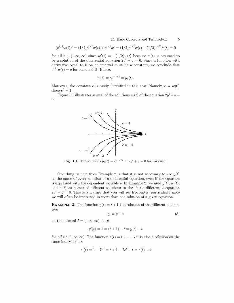
Figure 1.1 illustrates several of the solutions yc(t) of the equation 2y′+y =0.
t
y
c = 1
c = 2
c = 4
c = −1
c = −2
c = −4
Fig. 1.1. The solutions yc(t) = ce−t/2 of 2y′ + y = 0 for various c.
One thing to note from Example 2 is that it is not necessary to use y(t)as the name of every solution of a differential equation, even if the equationis expressed with the dependent variable y. In Example 2, we used y(t), yc(t),and w(t) as names of different solutions to the single differential equation2y′ + y = 0. This is a feature that you will see frequently, particularly sincewe will often be interested in more than one solution of a given equation.
Example 3. The function y(t) = t+ 1 is a solution of the differential equa-tion
y′ = y − t (8)
on the interval I = (−∞,∞) since
y′(t) = 1 = (t+ 1)− t = y(t)− t
for all t ∈ (−∞,∞). The function z(t) = t+ 1− 7et is also a solution on thesame interval since
z′(t) = 1− 7et = t+ 1− 7et − t = z(t)− t
6 1 Introduction
for all t ∈ (−∞.∞). Note that w(t) = y(t) − z(t) = 7et is not a solution of(8) since
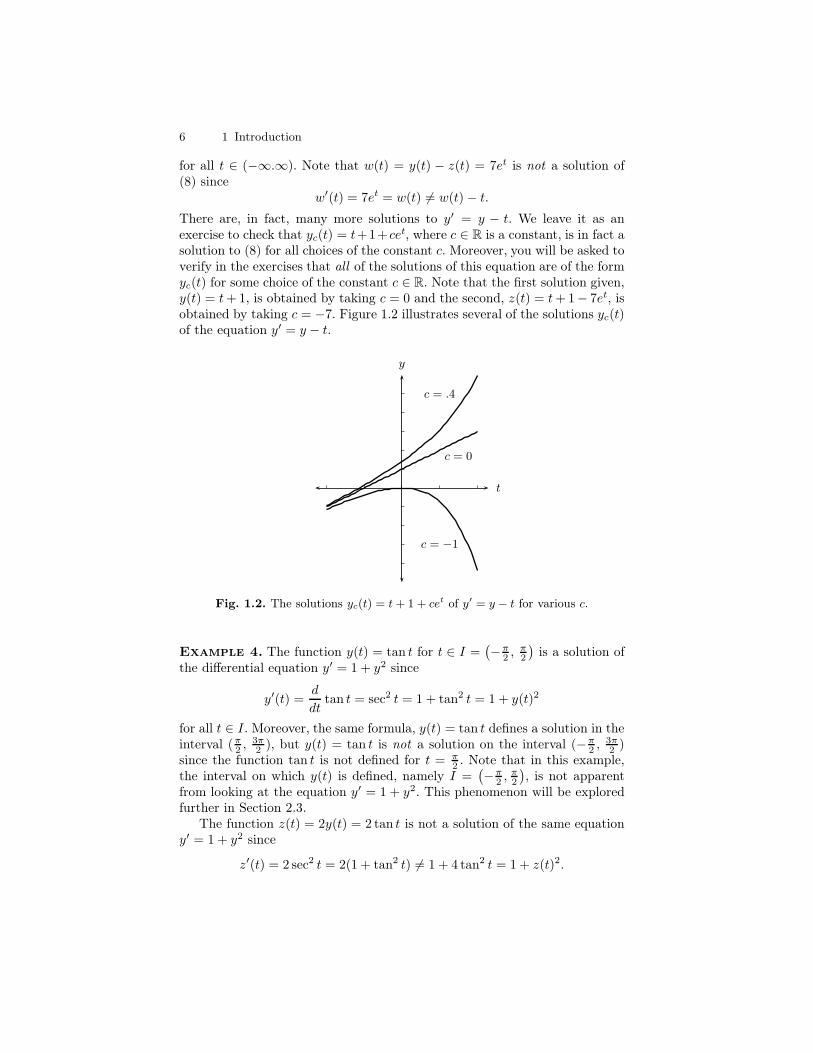
w′(t) = 7et = w(t) 6= w(t) − t.There are, in fact, many more solutions to y′ = y − t. We leave it as anexercise to check that yc(t) = t+1+cet, where c ∈ R is a constant, is in fact asolution to (8) for all choices of the constant c. Moreover, you will be asked toverify in the exercises that all of the solutions of this equation are of the formyc(t) for some choice of the constant c ∈ R. Note that the first solution given,y(t) = t+ 1, is obtained by taking c = 0 and the second, z(t) = t+ 1− 7et, isobtained by taking c = −7. Figure 1.2 illustrates several of the solutions yc(t)of the equation y′ = y − t.
t
y
c = 0
c = −1
c = .4
Fig. 1.2. The solutions yc(t) = t + 1 + cet of y′ = y − t for various c.
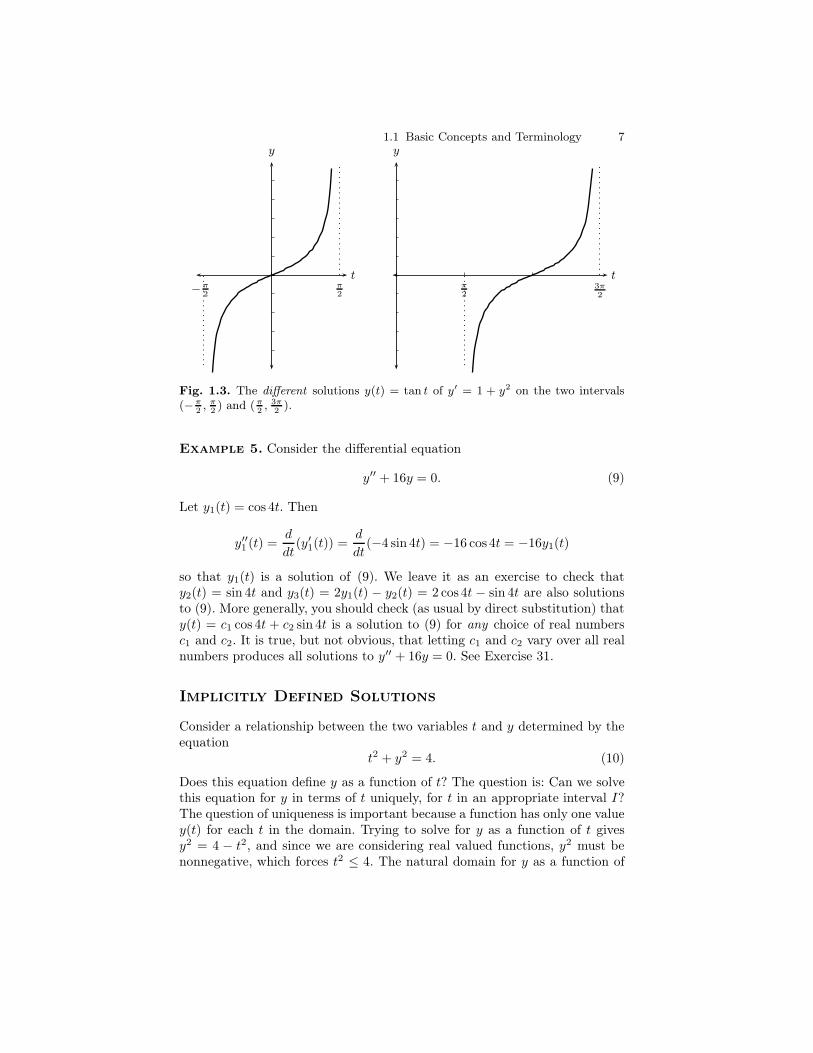
Example 4. The function y(t) = tan t for t ∈ I =(
−π2 ,
π2
)
is a solution ofthe differential equation y′ = 1 + y2 since
y′(t) =d
dttan t = sec2 t = 1 + tan2 t = 1 + y(t)2
for all t ∈ I. Moreover, the same formula, y(t) = tan t defines a solution in theinterval (π
2 ,3π2 ), but y(t) = tan t is not a solution on the interval (−π
2 ,3π2 )
since the function tan t is not defined for t = π2 . Note that in this example,
the interval on which y(t) is defined, namely I =(
−π2 ,
π2
)
, is not apparentfrom looking at the equation y′ = 1 + y2. This phenomenon will be exploredfurther in Section 2.3.
The function z(t) = 2y(t) = 2 tan t is not a solution of the same equationy′ = 1 + y2 since
z′(t) = 2 sec2 t = 2(1 + tan2 t) 6= 1 + 4 tan2 t = 1 + z(t)2.
1.1 Basic Concepts and Terminology 7
t
y
π2
−π2
t
y
π2
3π2
Fig. 1.3. The different solutions y(t) = tan t of y′ = 1 + y2 on the two intervals(−π
2, π
2) and (π
2, 3π
2).
Example 5. Consider the differential equation
y′′ + 16y = 0. (9)
Let y1(t) = cos 4t. Then
y′′1 (t) =d
dt(y′1(t)) =
d
dt(−4 sin 4t) = −16 cos 4t = −16y1(t)
so that y1(t) is a solution of (9). We leave it as an exercise to check thaty2(t) = sin 4t and y3(t) = 2y1(t) − y2(t) = 2 cos 4t − sin 4t are also solutionsto (9). More generally, you should check (as usual by direct substitution) thaty(t) = c1 cos 4t + c2 sin 4t is a solution to (9) for any choice of real numbersc1 and c2. It is true, but not obvious, that letting c1 and c2 vary over all realnumbers produces all solutions to y′′ + 16y = 0. See Exercise 31.
Implicitly Defined Solutions
Consider a relationship between the two variables t and y determined by theequation
t2 + y2 = 4. (10)
Does this equation define y as a function of t? The question is: Can we solvethis equation for y in terms of t uniquely, for t in an appropriate interval I?The question of uniqueness is important because a function has only one valuey(t) for each t in the domain. Trying to solve for y as a function of t givesy2 = 4 − t2, and since we are considering real valued functions, y2 must benonnegative, which forces t2 ≤ 4. The natural domain for y as a function of
8 1 Introduction
t determined by (10) is thus I = [−2, 2], and we have two equally deservingcandidates for y(t):
y1(t) =√
4− t2 or y2(t) = −√
4− t2.
Of course, you will recognize immediately that the graph of y1(t) is the upperhalf of the circle of radius 2 centered at the origin of the (t, y)-plane, whilethe graph of y2(t) is the lower half. We will say that either of the functionsy1(t) or y2(t) is defined implicitly by the equation t2 + y2 = 4. This meansthat
t2 + (y1(t))2 = 4 for all t ∈ I,
and similarly for y2(t). If this last equation is differentiated with respect tothe independent variable t, we get
2t+ 2y1(t)y′1(t) = 0 for all t ∈ I,
and similarly for y2(t). That is, both functions y1(t) and y2(t) implicitly definedby (10) are solutions to the same differential equation
t+ yy′ = 0. (11)
Moreover, if we change the constant 4 to any other positive constant r, implicitdifferentiation of the implicit equation t2 + y2 = r with respect to t givesthe same differential equation t + yy′ = 0 (after dividing by 2). Thus all ofthe infinitely many functions implicitly defined by the family of equationst2 + y2 = r, as r varies over the positive real numbers, are solutions of thesame differential equation (11).
The analysis of the previous paragraph remains true for any family ofimplicitly defined functions. If f(t, y) is a function of two variables, we willsay that a function y(t) defined on an interval I is implicitly defined by theequation
f(t, y) = r,
where r is a fixed real number if
f(t, y(t)) = r for all t ∈ I. (12)
This is a precise expression of what we mean by the statement:
Solve the equation f(t, y) = r for y as a function of t.
Since, as we have seen with the equation t2 + y2 = r, the equation f(t, y) = rmay have more than one way to solve for y as a function of t, and hence thesame two variable function f(t, y) can determine more than one implicitlydefined function y(t) from the same constant r. It can determine infinitelymany different implicitly defined functions if we let the constant r be chosen
1.1 Basic Concepts and Terminology 9
from an infinite subset of R. By differentiating (12) with respect to t (usingthe chain rule from multiple variable calculus), we find
∂f
∂t(t, y(t)) +
∂f
∂y(t, y(t))y′(t) = 0.
Since the constant r is not present in this equation, we conclude that everyfunction implicitly defined by the equation f(t, y) = r, for any constant r, isa solution of the same first order differential equation
∂f
∂t+∂f
∂yy′ = 0. (13)
We shall refer to (13) as the differential equation for the family of curvesf(t, y) = r. One valuable technique that we will encounter in Chapter 2 isto solve a first order differential equation by recognizing it as the differentialequation of a particular family of curves.
Example 6. Find the first order differential equation for the family of hy-perbolas ty = r in the (t, y)-plane.
I Solution. The defining function for the family of curves is f(t, y) = ty so(13) gives
∂f
∂t+∂f
∂yy′ = y + ty′ = 0
as the differential equation for this family. In standard form this equation isy′ = −y/t. Notice that this agrees with expectations, since for this simplefamily ty = r, we can solve explicitly to get y = r/t (for t 6= 0) so thaty′ = −r/t2 = −y/t. J
Initial Value Problems
As we have seen in the examples of differential equations and their solutionspresented in this section, differential equations generally have infinitely manysolutions so to specify a particular solution of interest, it is necessary to specifyadditional data. What is usually convenient to specify is an initial value y(t0)for a first order equation and an initial value y(t0) and an initial derivativey′(t0) in the case of a second order equation, with obvious extensions to higherorder equations. When the differential equation and initial values are specified,then one obtains what is known as an initial value problem. Thus a firstorder initial value problem in standard form is
y′ = F (t, y), y(t0) = y0 (14)
while a second order equation in standard form is written
y′′ = F (t, y, y′), y(t0) = y0, y′(t0) = y1. (15)
10 1 Introduction
Example 7. Determine a solution to each of the following initial value prob-lems
1. y′ = y − t, y(0) = −3.2. y′′ = 2− 6t, y(0) = −1, y′(0) = 2.
I Solution. 1. Recall from Example 3 that for each c ∈ R, the functionyc(t) = t+ 1 + cet is a solution for y′ = y− t. Thus our strategy is just totry to match one of the yc(t) with the required initial condition y(0) = −3.Thus
−3 = yc(0) = 1 + ce0 = 1 + c
requires that we take c = −4. Hence,
y(t) = y−4(t) = t+ 1− 4et
is a solution of the initial value problem.2. The second equation is asking for a function y(t) whose second derivative
is the given function 2 − t. But this is precisely the type of problem thatyou learned to solve in calculus using integration. Integration of y′′ gives
y′(t)− y′(0) =
∫ t
0
y′′(x) dx =
∫ t
0
(2 − 6x) dx = 2t− 3t2,
so that y′(t) = y(0) + 2t− 3t2 = 2 + 2t− 3t2. Note that we have used thevariable x in the integral, since the variable t appears in the limits of theintegral. Now integrate again to get
y(t)− y(0) =
∫ t
0
y′(x) dx =
∫ t
0
(2 + 2x− 3x2) dx = 2t+ t2 − t3.
Hence we get y(t) = −1 + 2t+ t2 − t3 as the solution of our second orderinitial value problem. J
Exercises
1. What is the order of each of the following differential equations?
(a) y2y′ = t3 (b) y′y′′ = t3
(c) t2y′ + ty = et (d) t2y′′ + ty′ + 3y = 0
(e) 3y′ + 2y + y′′ = t2 (f) t(y(4))3 + (y′′′)4 = 1(g) y′ + t2y = ty4 (h) y′′′ − 2y′′ + 3y′ − y = 0
Determine whether each of the given functions yj(t) is a solution of the corre-sponding differential equation.
2. y′ = 2y: y1(t) = 0, y2(t) = t2, y3(t) = 3e2t, y4(t) = 2e3t.3. y′ = 2y − 10: y1(t) = 5, y2(t) = 0, y3(t) = 5e2t, y4(t) = e2t + 5.4. ty′ = y: y1(t) = 0, y2(t) = 3t, y3(t) = −5t, y4(t) = t3.5. y′′ + 4y = 0: y1(t) = e2t, y2(t) = sin 2t, y3(t) = cos(2t − 1), y4(t) = t2.
1.1 Basic Concepts and Terminology 11
Verify that each of the given functions y(t) is a solution of the given differentialequation on the given interval I . Note that all of the functions depend on an arbitraryconstant c ∈ R.
6. y′ = 3y + 12; y(t) = ce3t − 4, I = (−∞,∞)7. y′ = −y + 3t; y(t) = ce−t + 3t − 3 I = (−∞,∞)8. y′ = y2 − y; y(t) = 1/(1 − cet) I = (−∞,∞) if c < 0, I = (− ln c, ∞) if
c > 09. y′ = 2ty; y(t) = cet2 , I = (−∞,∞)
10. (t + 1)y′ + y = 0; y(t) = c(t + 1)−1, I = (−1,∞)11. y′ = y2; y(t) = (c − t)−1, I = (−∞, c)
Find the general solution of each of the following differential equations by in-tegration. See the solution of Equation (2) in Example 7 for an example of thistechnique.
12. y′ = t + 3 13. y′ = e2t − 1 14. y′ = te−t
15. y′ =t + 1
t16. y′′ = 2t + 1 17. y′′ = 6 sin 3t
Find a solution to each of the following initial value problems. See Exercises6 through 17 for the general solutions of these equations, and see the solution ofEquation (1) in Example 7 for an example of the technique of finding a solution ofan initial value problem from the knowledge of a general family of solutions.
18. y′ = 3y + 12, y(0) = −2 19. y′ = −y + 3t, y(0) = 0
20. y′ = y2 − y, y(0) = 1/2 21. (t + 1)y′ + y = 0, y(1) = −9
22. y′ = e2t − 1, y(0) = 4 23. y′ = te−t, y(0) = −1
24. y′′ = 6 sin 3t, y(0) = 1, y′(0) = 2
Find the first order differential equation for each of the following families ofcurves. In each case c denotes an arbitrary real constant. See Example 6.
25. 3t2 + 4y2 = c 26. y2 − t2 − t3 = c
27. y = ce2t + t 28. y = ct3 + t2
29. Show that every solution of the equation y′ = ky, where k ∈ R, is one of thefunctions yc(t) = cekt, where c is an arbitrary real constant.Hint: See the second paragraph of Example 2.
30. In Example 3 it was shown that every function yc(t) = t + 1 + cet, where c ∈ R
is a solution of the differential equation y′ = y − t. Show that if y(t) is any
solution of y′ = y − t, then y(t) = yc(t) for some constant c.Hint: Show that z(t) = y(t) − t − 1 is a solution of the differential equationy′ = y and apply the previous exercise.
31. If k is a positive real number, use the following sequence of steps to show thatevery solution y(t) of the second order differential equation y′′ + k2y = 0 hasthe form
y(t) = c1 cos kt + c2 sin kt
for arbitrary real constants c1 and c2.
12 1 Introduction
(a) Show that each of the functions y(t) = c1 cos kt + c2 sin kt satisfies thedifferential equation y′′ + k2y = 0.
(b) Given real numbers a and b, show that there exists a solution of the initialvalue problem
y′′ + k2y = 0, y(0) = a, y′(0) = b.
(c) If y(t) is any solution of y′′ + k2y = 0, show that the function E(t) =(ky(t))2 + (y′(t))2 is constant. Conclude that E(t) = (ky(0))2 + (y′(0))2 forall t ∈ R, and hence, if y(0) = y′(0) = 0, then E(t) = 0 for all t. Concludethat if y(0) = y′(0) = 0, then y(t) = 0 for all t.
(d) Given real numbers a and b, show that there exists exactly one solution ofthe initial value problem
y′′ + k2y = 0, y(0) = a, y′(0) = b.
1.2 Examples of Differential Equations
As we have observed in the previous section, the rules, or physical laws, gov-erning a quantity are frequently expressed mathematically as a relationshipbetween the instantaneous rate of change of the quantity and the value ofthe quantity. If t denotes time and y(t) denotes the value at time t of thequantity we wish to describe, then the instantaneous rate of change of y is thederivative y′(t). Thus, a relation between the instantaneous rate of change ofy and the value of y is expressed by an equation
f(y(t), y′(t)) = 0. (1)
This is a first order differential equation in which the time variable (or inde-pendent variable) does not appear explicitly. An equation in which the timevariable does not appear explicitly is said to be autonomous. Frequently, therelation between y(t) and y′(t) will also depend on the time t. In this case thedifferential equation has the form
f(t, y(t), y′(t)) = 0. (2)
In the following examples, we will show how to use some basic physicallaws to arrive at differential equations like (2) that can serve as models ofphysical processes. Some of the resulting differential equations will be easyto solve using the simple observations of the previous section; others willrequire the techniques developed in later chapters. Our goal at the momentis the modeling process itself, not the solutions. The first example will be thefalling body problem, as it was understood by the seventeenth century Italianscientist Galileo Galilei (1564 – 1642).
1.2 Examples of Differential Equations 13
The falling body problem
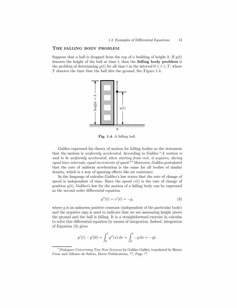
Suppose that a ball is dropped from the top of a building of height h. If y(t)denotes the height of the ball at time t, then the falling body problem isthe problem of determining y(t) for all time t in the interval 0 ≤ t ≤ T , whereT denotes the time that the ball hits the ground. See Figure 1.4.
0
y(t)
hei
ght
=h
Fig. 1.4. A falling ball.
Galileo expressed his theory of motion for falling bodies as the statementthat the motion is uniformly accelerated. According to Galileo “A motion issaid to be uniformly accelerated, when starting from rest, it acquires, duringequal time-intervals, equal increments of speed."1 Moreover, Galileo postulatedthat the rate of uniform acceleration is the same for all bodies of similardensity, which is a way of ignoring effects like air resistance.
In the language of calculus Galileo’s law states that the rate of change ofspeed is independent of time. Since the speed v(t) is the rate of change ofposition y(t), Galileo’s law for the motion of a falling body can be expressedas the second order differential equation
y′′(t) = v′(t) = −g, (3)
where g is an unknown positive constant (independent of the particular body)and the negative sign is used to indicate that we are measuring height abovethe ground and the ball is falling. It is a straightforward exercise in calculusto solve this differential equation by means of integration. Indeed, integrationof Equation (3) gives
y′(t)− y′(0) =
∫ t
0
y′′(x) dx =
∫ t
0
−g dx = −gt.
1Dialogues Concerning Two New Sciences by Galileo Galilei, translated by HenryCrew and Alfonso de Salvio, Dover Publications, ??, Page ??
14 1 Introduction
Since y′(0) = v0, the initial velocity of the body, we find
y′(t) = −gt+ v0.
Integrating once more we obtain
y(t) = −g2t2 + v0t+ y0, (4)
where the constant y0 is the initial position y(0). If we just drop the ball,as we have postulated in the falling body problem, then the initial velocityv0 = 0, and since y(0) = h, the height of the building, the solution of ourproblem is
y(t) = −g2t2 + h. (5)
There remains the problem of computing the constant g, but there is anexperimental way to do this. Since T denotes the time when the ball hits theground, it follows that 0 = y(T ) = −gT 2/2 + h so that
g =2h
T 2. (6)
Experimental calculations have shown that g (known as the gravitationalconstant) has the value 32 ft/sec2 in the English system of units and the value9.8 m/sec2 in the metric system of units. Thus, using the English system ofunits, the height y(t) at time t of a ball released from an initial height of h ftwith an initial velocity of v0 ft/sec is given, assuming Galileo’s law of motion,by
y(t) = −16t2 + v0t+ h. (7)
Example 1. If a ball is dropped from a height h, what will be the speed atwhich it hits the ground?
I Solution. According to (6) the ball will hit the ground at time T =√
2h/g and the speed at this time is |y′(T )| = |−gT | = √2gh. J
Example 2. Suppose that a ball is tossed straight up with an initial velocityv0. Ignoring air resistance, how high will the ball go?
I Solution. Since the initial height h = 0, the equation of motion is y(t) =− g
2 t2 + v0t. The maximum height is obtained when the velocity is zero. But
v(t) = y′(t) = −gt + v0 so v(t) = 0 occurs when t = v0/g. At this time theheight is
y(v0/g) = −g2
(
v0g
)2
+ v0
(
v0g
)
=v20
2g.
For a numerical example, this says that a ball thrown straight up at an initialspeed of 40 ft/sec will reach a height of 402/64 = 25 ft. J
1.2 Examples of Differential Equations 15
Radioactive decay
Certain chemicals decompose into other substances at a rate that is propor-tional to the amount present. Such a decomposition process is referred to asradioactive decay and it is characterized by the mathematical model
y′ = −ky, (8)
where y(t) denotes the amount of chemical present at time t, and k is a positiveconstant called the decay constant.
The solution of the radioactive decay equation (8) is
y(t) = ce−kt (9)
where c is an arbitrary real constant. This can be seen by the same argumentused in Example 2 on Page 4 (see also Exercise 29 in Section 1.1). Specifically,if y(t) is any solution of (8), multiply by ekt to get a function z(t) = ekty(t).Differentiating and using the fact that y(t) is a solution of (8), gives
z′(t) = ekty′(t) + kekty(t) = −kekty(t) + kekty(t) = 0, for all t,
so that z(t) = c for some constant c ∈ R. Thus, y(t) = e−ktz(t) = ce−kt, asrequired.
If there is a quantity y0 = y(t0) of the radioactive chemical present at theinitial time t0, then the condition y0 = y(t0) = ce−kt0 gives the value of theconstant c = y0e
kt0 . Putting this value of c into (9) gives
y(t) = y0e−k(t−t0) (10)
for the amount present at time t, assuming that y0 is present at time t0.There is still the question of determining the proportionality constant k,
which depends on the particular substance being studied. Suppose we havemeasured the amount present at time t0, namely y0 and also the amountpresent at time t1 6= t0, say y1. Then
y1 = y(t1) = y0e−k(t1−t0),
and in this equation, all quantities are known except for k. Thus, we can solvethis equation for the unknown decay constant k. If we do the calculation, weget
k =1
t1 − t0ln(y0/y1). (11)
The conclusion is that if the value of a radioactive quantity is known attwo different times, then it is possible to compute, using equations (10) and(11), the quantity present at all future times. If, in this expression, we takey1 = y0/2 and let T = t1 − t0, then we get
16 1 Introduction
k =ln 2
T. (12)
That is, the decay constant can be computed if the time T that it takes thematerial to decay to one-half its original amount is known. This time is usuallyreferred to as the half-life of the radioactive material.
Example 3. The half-life of radium is 1620 years. What is the amount y(t)of radium remaining after t years if the initial quantity was y0? What per-centage of the original quantity will remain after 500 years?
I Solution. From (12) the decay constant is calculated to be k = ln 2/1620 ≈.000428. Thus y(t) = y0e
−.000428t. Note that we have taken the initialtime t0 to be 0. After 500 years, the amount remaining will be y(500) =y0e
−.000428×500 ≈ .807y0. Thus, after 500 years, approximately 80.7% of theoriginal amount of radium will still be present. J
Newton’s law of heating and cooling
Newton’s Law of heating and cooling states that the rate of changeof the temperature of an object is proportional to the difference between thetemperature of the object and the temperature of the surrounding medium. IfT (t) denotes the temperature of the object at time t and A is the temperatureof the surrounding medium (which will be assumed to be constant in thissimple case), then Newton’s law is expressed in mathematical language as thedifferential equation
dT
dt(t) = k(T (t)−A). (13)
If T (t) > A then the object will cool, so that dT/dt < 0, while if T (t) < A thenthe object will heat up toward the ambient temperature A, so that dT/dt > 0.In both cases, the proportionality constant k will be negative.
Letting y(t) = T (t) − A, and recalling that the temperature A of thesurrounding medium is assumed to be constant, (13) takes the form
y′ =d
dt(T −A) =
dT
dt= k(T −A) = ky. (14)
This is the same equation as the equation of radioactive decay (8), and we havealready observed (Equation (9)) that this equation has the solution y(t) =ce−kt where c = y(0). Thus, (13) has the solution
T (t) = A+ (T (0)−A)ekt. (15)
Example 4. A thin plate is placed in boiling water to be sterilized in prepa-ration for receiving a cell culture. The plate is removed from the boiling water(100C) and put in a 20C room to cool. After 5 min the plate has cooled to atemperature of 80C. The culture can be introduced when the temperature is30C. How much longer will it be necessary to wait before the plate is readyto receive the cell culture?
1.2 Examples of Differential Equations 17
I Solution. Let T (t) denote the temperature of the plate at time t, wheret = 0 corresponds to the time when the plate is removed from the boilingwater. Thus, we are assuming that the initial temperature is T (0) = 100 degC.In this example, the surrounding medium is the air in the room, which isassumed to have a temperature of A = 20 degC. According to Newton’s lawof cooling (Equation (13)) the differential equation governing the cooling ofthe plate is
dT
dt(t) = k(T (t)−A) = k(T (t)− 20),
which, according to (15) has the solution
T (t) = A+ (T (0)−A)ekt = 20 + 80ekt.
This will completely describe T (t), once the parameter k is determined, whichis accomplished by taking advantage of the fact that the temperature of theplate is 80 degC after 5 min, i.e., T (5) = 80. Thus,
80 = T (5) = 20 + 80e5k,
so that 60/80 = e5k which implies that k = .2 ln .75 = −.057536414. There-fore, the temperature of the plate at all times after it is removed from theboiling water is
T (t) = 20 + 80e−.057536414t.
We need the time at which the temperature is 30 degC, which we can deter-mine by solving for t in the equation
30 = T (t) = 20 + 80e−.057536414t.
Thus, e−.057536414t = 10/80 = .125 so
t =ln .125
−.057536414= 36.14 min.
Thus, the answer to the question asked is that since 5 min was needed it reach80 degC, it takes an additional 36.14 − 5 = 31.14 min to reach the desiredtemperature of 30 degC.
Mixing problems
Example 5. Consider a tank which contains 2000 gallons of water in which10 lbs of salt are dissolved. Suppose that brine (a water-salt mixture) with aconcentration of 0.1 lb/gal enters the tank at a rate of 2 gal/min, and assumethat the well-stirred mixture flows from the tank at the same rate of 2 gal/min.Find the amount y(t) of salt (expressed in pounds) which is present in thetank at all times t, measured in minutes after the initial time (t = 0) when 10lbs are present.
18 1 Introduction
I Solution. This is another example of where it is easier to describe howy(t) changes, that is y′(t), than it is to directly describe y(t). Since the de-scription of y′(t) will also include y(t), a differential equation will result. Startby noticing that at time t0, y(t0) lbs of salt are present and at a later time t,the amount of salt in the tank is given by
y(t) = y(t0) +A(t0, t)− S(t0, t) (16)
where A(t0, t) is the amount of salt added between times t0 and t and S(t0, t)is the amount removed between times t0 and t. To compute A(t0, t) note that
A(t0, t) = cin(t)rin(t)∆t
where
cin(t) = concentration of salt solution being added = 0.1 lb/gal
rin(t) = volume rate of salt solution being added = 2 gal/min
∆t = t− t0 = time interval between t0 and t,
so thatA(t0, t) = (0.1)× (2)×∆t. (17)
By exactly the same reasoning,
S(t0, t) = cout(t)rout(t)∆t
where
cout(t) = concentration of salt solution being removed
rout(t) = volume rate of salt solution being removed
∆t = t− t0 = time interval between t0 and t.
The number of gallons per minute flowing out of the tank is the same as therate flowing in, namely, 2 gal/min, so that rout = 2 gal/min. However, cout,the number of pounds per gallon being removed at any given time t will begiven by y(t)/V (t), that is divide the total number of pounds of salt in thetank at time t (namely y(t)) by the current total volume V (t) of solution inthe tank. In our case, V (t) is always 2000 gal (the flow in and the flow outbalance), but y(t) changes with time, and that is what we ultimately will wantto compute. If t is “close" to t0 then we can assume that y(t) ≈ y(t0) so that
S(t0, t) ≈(
y(t0)
2000lbs/gal
)
× (2 gal/min)×∆t. (18)
Combining (16), (17), and (18) gives
y(t)− y(t0) = A(t0, t)− S(t0, t)
≈ (0.2)(t− t0)− 2y(t0)
2000(t− t0).
1.2 Examples of Differential Equations 19
Dividing this by t− t0 and letting t→ t0 gives the equation
y′(t0) = 0.2− 1
1000y(t0),
which we recognize as a differential equation. Note that it is the process oftaking the limit as t→ t0 that allows us to return to an equation, rather thandealing only with an approximation. This is a manifestation of what we meanwhen we indicate that it is frequently easier to describe the way somethingchanges, that is y′(t), rather than “what is," i.e. y(t) itself.
Since t0 is an arbitrary time, we can write the above equation as a differ-ential equation
y′ = (0.2)− 1
1000y (19)
and it becomes an initial value problem by specifying that we want y(0) = 10,that is, there are 10 lbs of salt initially present in the tank.
The equation (19) is easily solved by factoring out −1/1000 = −10−3 torewrite it as
y′ = −10−3(y − 200). (20)
This is the same type of equation as Newton’s law of cooling (Equation (13)),where k = −10−3 and A = 200. Setting z = y − 200 transforms (20) into thebasic radioactive decay type equation z′ = −10−3z, which has the solutionz(t) = z(0)e−10−3t. Since y(t) = z(t) + 200 we get
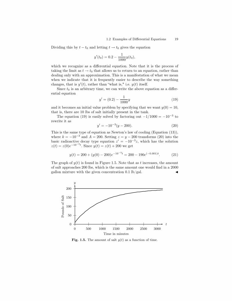
y(t) = 200 + (y(0)− 200)e−10−3t = 200− 190e(−0.001)t. (21)
The graph of y(t) is found in Figure 1.5. Note that as t increases, the amountof salt approaches 200 lbs, which is the same amount one would find in a 2000gallon mixture with the given concentration 0.1 lb/gal. J
0
50
100
150
200
0 500 1000 1500 2000 2500 3000
t
y
Pou
nds
ofSal
t
Time in minutes
Fig. 1.5. The amount of salt y(t) as a function of time.
20 1 Introduction
The following example summarizes a slightly more general situation thanthat covered by the previous numerical example. It will lead to a differentialequation (23) more general than the equation y′ = ay + b, where a and bare constants, that has characterized all the examples so far presented. Thesolution of equations of this type will be described in the next chapter.
Example 6 (Mixing problem). A tank initially holds V0 gal of brine(awater-salt mixture) that contains a lb of salt. Another brine solution, contain-ing c lb of salt per gallon, is poured into the tank at a rate of r gal/min. Themixture is stirred to maintain uniformity of concentration of salt at all partsof the tank, and the stirred mixture flows out of the tank at the rate of Rgal/min. Let y(t) denote the amount of salt (measured in pounds) in the tankat time t. Find an initial value problem for y(t).
I Solution. We are searching for an equation which describes the rate ofchange of the amount of salt in the tank at time t, i.e., y′(t). The key observa-tion, which we shall refer to as the balance equation, is that this rate of changeis the difference between the rate at which salt is being added to the tank andthe rate at which the salt is being removed from the tank. In symbols:
y′(t) = Rate in− Rate out. (22)
The rate that salt is being added is easy to compute. It is rc lb/min (c lb/gal× r gal/min = rc lb/min). Note that this is the appropriate units for a rate,namely an amount divided by a time. We still need to compute the rate atwhich salt is leaving the tank. To do this we first need to know the number ofgallons V (t) of brine in the tank at time t. But this is just the initial volumeplus the amount added up to time t minus the amount removed up to time t.That is, V (t) = V0 + rt −Rt = V0 + (r −R)t. Since y(t) denotes the amountof salt present in the tank at time t, the concentration of salt at time t isy(t)/V (t) = y(t)/(V0 − (r − R)t), and the rate at which salt leaves the tankis R× y(t)/V (t) = Ry(t)/(V0 + (r −R)t). Thus,
y′(t) = Rate in− Rate out
= rc− R
V0 + (r −R)ty(t)
In the standard form of a linear differential equation, the equation for the rateof change of y(t) is
y′(t) +R
V0 + (r −R)ty(t) = rc. (23)
This becomes an initial value problem by remembering that y(0) = a. As inthe previous example, this is a first order linear differential equation, and thesolutions will be studied in Section 2.2. J
1.2 Examples of Differential Equations 21
Remark 7. You should definitely not memorize a formula like Equation (23).What you should remember is how it was set up so that you can set up yourown problems, even if the circumstances are slightly different from the onegiven above. As one example of a possible variation, you might encounter asituation in which the volume V (t) varies in a nonlinear manner such as, forexample, V (t) = 5 + 3e−2t.
Electric Circuits
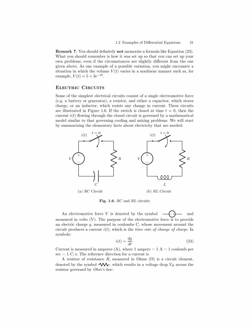
Some of the simplest electrical circuits consist of a single electromotive force(e.g. a battery or generator), a resistor, and either a capacitor, which storescharge, or an inductor, which resists any change in current. These circuitsare illustrated in Figure 1.6. If the switch is closed at time t = 0, then thecurrent i(t) flowing through the closed circuit is governed by a mathematicalmodel similar to that governing cooling and mixing problems. We will startby summarizing the elementary facts about electricity that are needed.
V
t = 0i(t)
R
C
+
−
(a) RC Circuit
V
t = 0i(t)
R
L
+
−
(b) RL Circuit
Fig. 1.6. RC and RL circuits
An electromotive force V is denoted by the symbol +− and
measured in volts (V). The purpose of the electromotive force is to providean electric charge q, measured in coulombs C, whose movement around thecircuit produces a current i(t), which is the time rate of change of charge. Insymbols:
i(t) =dq
dt. (24)
Current is measured in amperes (A), where 1 ampere = 1 A = 1 coulomb persec = 1 C/s. The reference direction for a current is
A resistor of resistance R, measured in Ohms (Ω) is a circuit element,denoted by the symbol , which results in a voltage drop VR across theresistor governed by Ohm’s law :
22 1 Introduction
VR = Ri(t). (25)
The capacitor, denoted and measured in units of Farads (F) storescharge, and in doing so results in a voltage drop VC across the capacitor C.The charge stored q(t) is proportional to the voltage drop VC :
q(t) = CVC . (26)
An inductor of inductance L is a circuit element denoted by the symboland measured in Henrys (H), that resists changes in the current i(t).
This is manifested by a voltage drop VL that is proportional to the rate ofchange of current:
VL = Ldi
dt. (27)
In the simple RC (resistor-capacitor) and RL (resistor-inductor) circuitsconsidered here, the resistance R, capacitance C and inductance L are con-stants while the electromotive force will be an applied voltage that could beeither constant, such as supplied by a battery, or time-varying such as thatfound in an alternating current circuit. The fundamental physical law thatgoverns voltage drops around a closed circuit is Kirchhoff’s voltage law:
The algebraic sum of the voltage drops around any closed loop is 0. (28)
Let us apply the basic principles expressed by Equations (24) – (28) tothe circuits of Figures 1.6 (a) and (b) to see how they lead to differentialequations governing the movement of charge around the closed circuit, oncethe switch has been closed at time t = 0. In the RC circuit of Figure 1.6 (a),there are voltage drops VR across the resistor and VC across the capacitor,while the electromotive force V provides a positive voltage, which correspondsto a voltage drop of −V . Kirchhoff’s voltage law then gives
VR + VC − V = 0.
Using Ohm’s law (25) and the capacitor proportionality rule (26), this givesan equation
Ri(t) +q(t)
C= V,
and recalling that current i(t) is the time rate of change of charge, we arriveat the differential equation
Rdq
dt+q
C= V. (29)
This differential equation describes the movement of charge around the circuitin Figure 1.6 (a).
The RL circuit in Figure 1.6 (b) is treated similarly. Kirchhoff’s law givesthe equation
1.2 Examples of Differential Equations 23
VR + VL = V
and applying Ohm’s law and the inductor proportionality equation (27) givesa differential equation
Ldi
dt+Ri = V. (30)
Note that the differential equation (29) determined by the RC circuit of Figure1.6 (a) is a differential equation for the charge q(t), while the equation (30)determined by the RL circuit of Figure 1.6 (b) is a differential equation forthe current i(t). However, if the applied voltage is a constant V , then both ofthese equations have the basic form
ay′ + by = c
where a, b, and c are constants. Note that this is exactly like the equationsconsidered earlier in this section.
We will conclude by considering a couple of numerical equations of thetype involved in studying RC and RL circuits. Numerical examples
here.1. How long does it take a ball dropped from the top of a 400 ft tower to reach
the ground? What will be the speed when it hits the ground?
2. A ball is thrown straight up from the top of a building of height h. If the initialvelocity is v0 (and ignoring air resistance), how long will it take to reach themaximum height? How long will it take to reach the ground?
3. A ball is thrown straight up from the ground with an initial velocity of 25meters/sec. There will be two times when the ball is at a height of 15 meters.Find those two times.
4. On planet P the following experiment is performed. A small rock is droppedfrom a height of 4 feet and it is observed that it hits the ground in 1 sec.Suppose another stone is dropped from a height of 1000 feet. What will be theheight after 5 sec.? How long will it take for the stone to hit the ground?
5. Radium decomposes at a rate proportional to the amount present. Express thisproportionality statement as a differential equation for R(t), the amount ofradium present at time t.
6. Bacteria are placed in a sugar solution at time t = 0. Assuming adequate foodand space for growth, the bacteria will grow at a rate proportional to the currentpopulation of bacteria. Write a differential equation satisfied by the number P (t)of bacteria present at time t.
7. Continuing with the last exercise, assume that the food source for the bacteriais adequate, but that the colony is limited by space to a maximum populationM . Write a differential equation for the population P (t) which expresses theassumption that the growth rate of the bacteria is proportional to the productof the number of bacteria currently present and the difference between M andthe current population.
24 1 Introduction
8. If a bottle of your favorite beverage is at room temperature (say 70 F) and itis then placed in a tub of ice at time t = 0, use Newton’s law of cooling to writean initial value problem which is satisfied by the temperature T (t) of the bottleat time t.
9. A turkey, which has an initial temperature of 40 (Fahrenheit), is placed into a350 oven. After one hour the temperature of the turkey is 120. Use Newton’sLaw of heating and cooling to find (1) the temperature of the turkey after 2hours, and (2) how many hours it takes for the temperature of the turkey toreach 250.
10. A cup of coffee, brewed at 180 (Fahrenheit), is brought into a car with in-side temperature 70. After 3 minutes the coffee cools to 140. What is thetemperature 2 minutes later?
11. The temperature outside a house is 90 and inside it is kept at 65. A ther-mometer is brought from the outside reading 90 and after 10 minutes it reads85. How long will it take to read 75? What will the thermometer read afteran hour?
12. A cold can of soda is taken out of a refrigerator with a temperature of 40 andleft to stand on the countertop where the temperature is 70. After 2 hours thetemperature of the can is 60. What was the temperature of the can 1 hourafter it was removed from the refrigerator?
13. A large cup hot of coffee is bought from a local drive through restaurant andplaced in a cup holder in a vehicle. The inside temperature of the vehicle is70 Fahrenheit. After 5 minutes the driver spills the coffee on himself a receivesa severe burn. Doctors determine that to receive a burn of this severity, thetemperature of the coffee must have been about 150. If the temperature of thecoffee was 142 6 minutes after it was sold what was the temperature at whichthe restaurant served it.
14. A student wishes to have some friends over to watch a football game. She wantsto have cold beer ready to drink when her friends arrive at 4 p.m. According toher tastes the temperature of beer can be served when its temperature is 50.Her experience shows that when she places 80 beer in the refrigerator that iskept at a constant temperature of 40 it cools to 60 in an hour. By what timeshould she put the beer in the refrigerator to ensure that it will be ready forher friends?
1.3 Direction Fields
The geometric interpretation of the derivative of a function y(t) at t0 as theslope of the tangent line to the graph of y(t) at (t0, y(t0)) provides us with anelementary and often very effective method for the visualization of the solu-tion curves (:= graphs of solutions) for a first order differential equation. Thevisualization process involves the construction of what is known as a direc-tion field or slope field for the differential equation. For this constructionwe proceed as follows.
1.3 Direction Fields 25
Construction of Direction Fields
(1) If the equation is not already in standard form (Equation (5)) solve theequation for y′ to put it in the standard form y′ = F (t, y).
(2) Choose a grid of points in a rectangle R = (t, y) : a ≤ t ≤ b; c ≤ y ≤ din the (t, y)-plane.
(3) At each grid point (t, y), the number F (t, y) represents the slope of asolution curve through this point; for example if y′ = y2 − t so thatF (t, y) = y2 − t, then at the point (1, 1) the slope is F (1, 1) = 12 − 1 = 0,at the point (2, 1) the slope is F (2, 1) = 12 − 2 = −1, and at the point(1,−2) the slope is F (1,−2) = 3.
(4) Through the point (t, y) draw a small line segment having the slope F (t, y).Thus, for the equation y′ = y2 − t, we would draw a small line segment ofslope 0 through (1, 1), slope −1 through (2, 1) and slope 3 through (1,−2).With a graphing calculator, one of the computer mathematics programsMaple, Mathematica or MATLAB (which we refer to as the three M’s)2, or with pencil, paper, and a lot of patience, you can draw many suchline segments. The resulting picture is called a direction field for thedifferential equation y′ = F (t, y).
(5) With some luck with respect to scaling and the selection of the (t, y)-rectangleR, you will be able to visualize some of the line segments runningtogether to make a graph of one of the solution curves.
(6) To sketch a solution curve of y′ = F (t, y) from a direction field, startwith a point P0 = (t0, y0) on the grid, and sketch a short curve throughP0 with tangent slope F (t0, y0). Follow this until you are at or close toanother grid point P1 = (t1, y1). Now continue the curve segment by usingthe updated tangent slope F (t1, y1). Continue this process until you areforced to leave your sample rectangle R. The resulting curve will be anapproximate solution to the initial value problem y′ = F (t, y), y(t0) = y0.
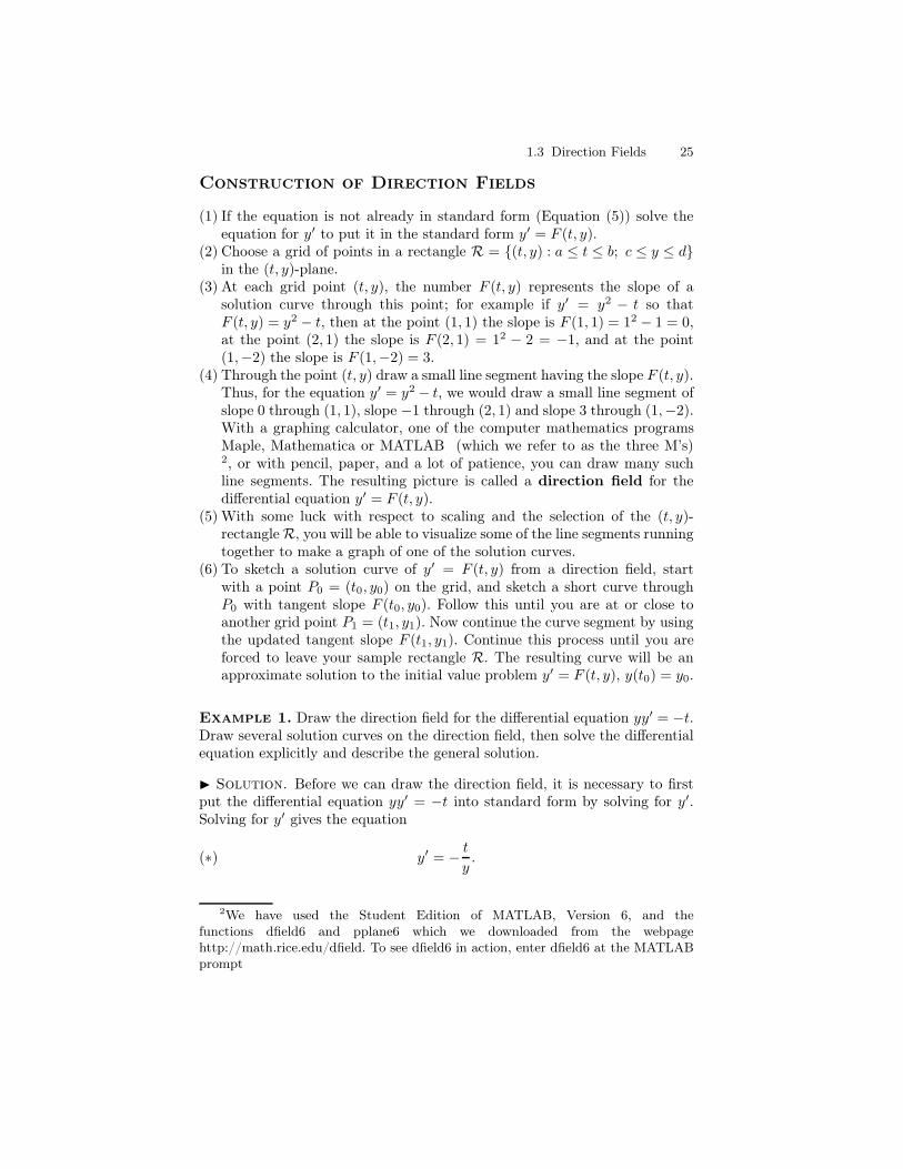
Example 1. Draw the direction field for the differential equation yy′ = −t.Draw several solution curves on the direction field, then solve the differentialequation explicitly and describe the general solution.
I Solution. Before we can draw the direction field, it is necessary to firstput the differential equation yy′ = −t into standard form by solving for y′.Solving for y′ gives the equation
(∗) y′ = − ty.
2We have used the Student Edition of MATLAB, Version 6, and thefunctions dfield6 and pplane6 which we downloaded from the webpagehttp://math.rice.edu/dfield. To see dfield6 in action, enter dfield6 at the MATLABprompt
26 1 Introduction
−4 −2 0 2 4
−4
−3
−2
−1
0
1
2
3
4
t
y
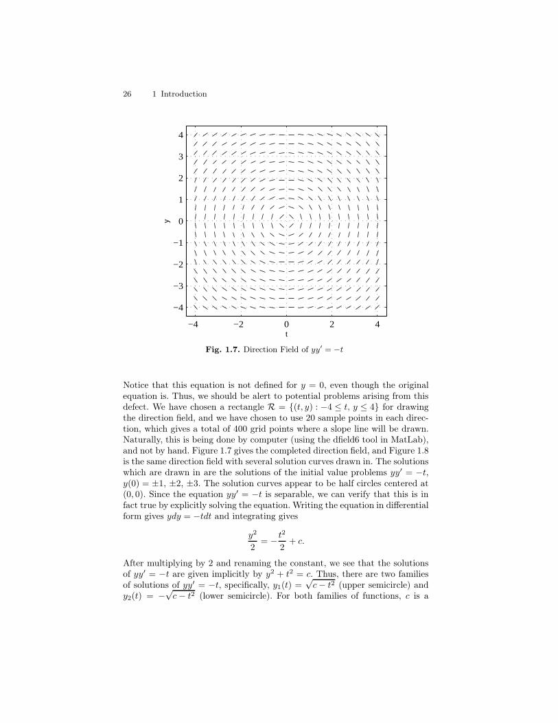
Fig. 1.7. Direction Field of yy′ = −t
Notice that this equation is not defined for y = 0, even though the originalequation is. Thus, we should be alert to potential problems arising from thisdefect. We have chosen a rectangle R = (t, y) : −4 ≤ t, y ≤ 4 for drawingthe direction field, and we have chosen to use 20 sample points in each direc-tion, which gives a total of 400 grid points where a slope line will be drawn.Naturally, this is being done by computer (using the dfield6 tool in MatLab),and not by hand. Figure 1.7 gives the completed direction field, and Figure 1.8is the same direction field with several solution curves drawn in. The solutionswhich are drawn in are the solutions of the initial value problems yy′ = −t,y(0) = ±1, ±2, ±3. The solution curves appear to be half circles centered at(0, 0). Since the equation yy′ = −t is separable, we can verify that this is infact true by explicitly solving the equation. Writing the equation in differentialform gives ydy = −tdt and integrating gives
y2
2= − t
2
2+ c.
After multiplying by 2 and renaming the constant, we see that the solutionsof yy′ = −t are given implicitly by y2 + t2 = c. Thus, there are two familiesof solutions of yy′ = −t, specifically, y1(t) =
√c− t2 (upper semicircle) and
y2(t) = −√c− t2 (lower semicircle). For both families of functions, c is a
1.3 Direction Fields 27
−4 −2 0 2 4
−4
−3
−2
−1
0
1
2
3
4
t
y
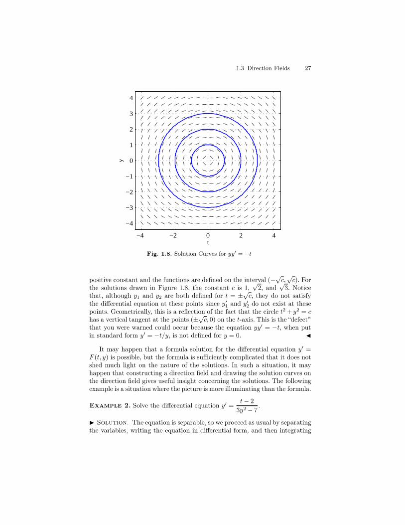
Fig. 1.8. Solution Curves for yy′ = −t
positive constant and the functions are defined on the interval (−√c,√c). Forthe solutions drawn in Figure 1.8, the constant c is 1,
√2, and
√3. Notice
that, although y1 and y2 are both defined for t = ±√c, they do not satisfythe differential equation at these points since y′1 and y′2 do not exist at thesepoints. Geometrically, this is a reflection of the fact that the circle t2 + y2 = chas a vertical tangent at the points (±√c, 0) on the t-axis. This is the “defect"that you were warned could occur because the equation yy′ = −t, when putin standard form y′ = −t/y, is not defined for y = 0. J
It may happen that a formula solution for the differential equation y′ =F (t, y) is possible, but the formula is sufficiently complicated that it does notshed much light on the nature of the solutions. In such a situation, it mayhappen that constructing a direction field and drawing the solution curves onthe direction field gives useful insight concerning the solutions. The followingexample is a situation where the picture is more illuminating than the formula.
Example 2. Solve the differential equation y′ =t− 2
3y2 − 7.
I Solution. The equation is separable, so we proceed as usual by separatingthe variables, writing the equation in differential form, and then integrating
28 1 Introduction
−4 −2 0 2 4 6 8
−5
0
5
t
y
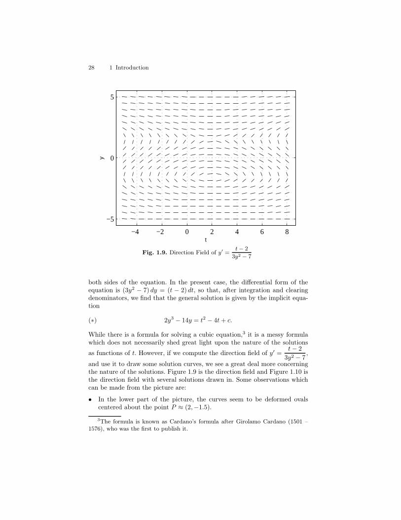
Fig. 1.9. Direction Field of y′ =t − 2
3y2 − 7
both sides of the equation. In the present case, the differential form of theequation is (3y2 − 7) dy = (t − 2) dt, so that, after integration and clearingdenominators, we find that the general solution is given by the implicit equa-tion
(∗) 2y3 − 14y = t2 − 4t+ c.
While there is a formula for solving a cubic equation,3 it is a messy formulawhich does not necessarily shed great light upon the nature of the solutions
as functions of t. However, if we compute the direction field of y′ =t− 2
3y2 − 7,
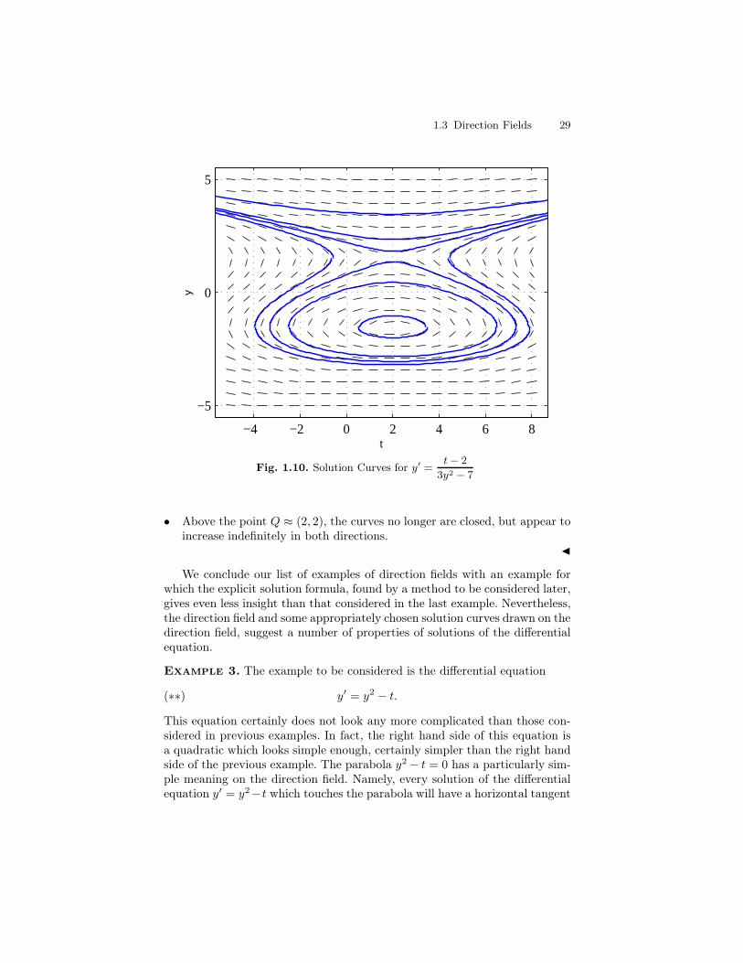
and use it to draw some solution curves, we see a great deal more concerningthe nature of the solutions. Figure 1.9 is the direction field and Figure 1.10 isthe direction field with several solutions drawn in. Some observations whichcan be made from the picture are:
• In the lower part of the picture, the curves seem to be deformed ovalscentered about the point P ≈ (2,−1.5).
3The formula is known as Cardano’s formula after Girolamo Cardano (1501 –1576), who was the first to publish it.
1.3 Direction Fields 29
−4 −2 0 2 4 6 8
−5
0
5
t
y
Fig. 1.10. Solution Curves for y′ =t − 2
3y2 − 7
• Above the point Q ≈ (2, 2), the curves no longer are closed, but appear toincrease indefinitely in both directions.
J
We conclude our list of examples of direction fields with an example forwhich the explicit solution formula, found by a method to be considered later,gives even less insight than that considered in the last example. Nevertheless,the direction field and some appropriately chosen solution curves drawn on thedirection field, suggest a number of properties of solutions of the differentialequation.
Example 3. The example to be considered is the differential equation
(∗∗) y′ = y2 − t.
This equation certainly does not look any more complicated than those con-sidered in previous examples. In fact, the right hand side of this equation isa quadratic which looks simple enough, certainly simpler than the right handside of the previous example. The parabola y2 − t = 0 has a particularly sim-ple meaning on the direction field. Namely, every solution of the differentialequation y′ = y2−t which touches the parabola will have a horizontal tangent
30 1 Introduction
at that point. That is, for every point (t0, y(t0)) on the graph of a solutiony(t) for which y(t0)
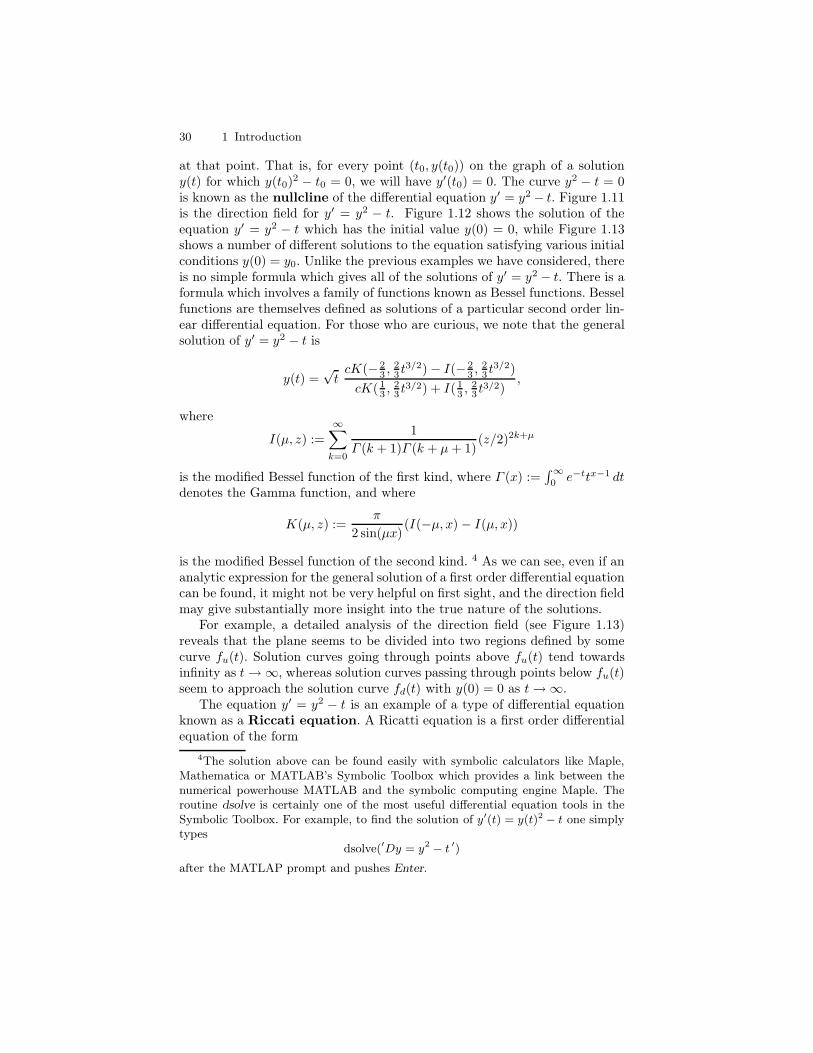
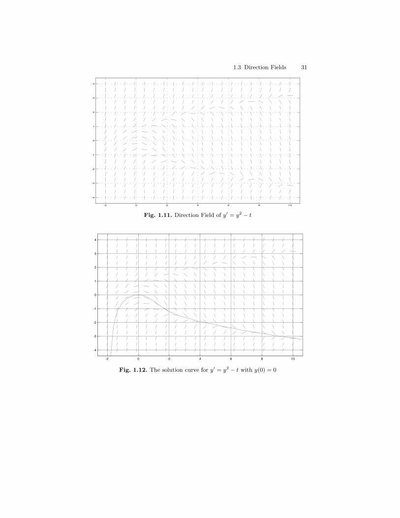
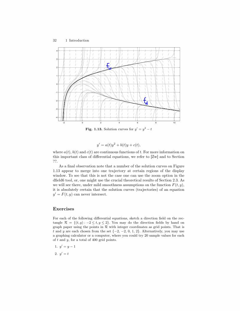
2 − t0 = 0, we will have y′(t0) = 0. The curve y2 − t = 0is known as the nullcline of the differential equation y′ = y2 − t. Figure 1.11is the direction field for y′ = y2 − t. Figure 1.12 shows the solution of theequation y′ = y2 − t which has the initial value y(0) = 0, while Figure 1.13shows a number of different solutions to the equation satisfying various initialconditions y(0) = y0. Unlike the previous examples we have considered, thereis no simple formula which gives all of the solutions of y′ = y2 − t. There is aformula which involves a family of functions known as Bessel functions. Besselfunctions are themselves defined as solutions of a particular second order lin-ear differential equation. For those who are curious, we note that the generalsolution of y′ = y2 − t is
y(t) =√tcK(− 2
3 ,23 t
3/2)− I(− 23 ,
23 t
3/2)
cK(13 ,
23 t
3/2) + I(13 ,
23 t
3/2),
where
I(µ, z) :=
∞∑
k=0
1
Γ (k + 1)Γ (k + µ+ 1)(z/2)2k+µ
is the modified Bessel function of the first kind, where Γ (x) :=∫∞0 e−ttx−1 dt
denotes the Gamma function, and where
K(µ, z) :=π
2 sin(µx)(I(−µ, x)− I(µ, x))
is the modified Bessel function of the second kind. 4 As we can see, even if ananalytic expression for the general solution of a first order differential equationcan be found, it might not be very helpful on first sight, and the direction fieldmay give substantially more insight into the true nature of the solutions.
For example, a detailed analysis of the direction field (see Figure 1.13)reveals that the plane seems to be divided into two regions defined by somecurve fu(t). Solution curves going through points above fu(t) tend towardsinfinity as t→∞, whereas solution curves passing through points below fu(t)seem to approach the solution curve fd(t) with y(0) = 0 as t→∞.
The equation y′ = y2 − t is an example of a type of differential equationknown as a Riccati equation. A Ricatti equation is a first order differentialequation of the form
4The solution above can be found easily with symbolic calculators like Maple,Mathematica or MATLAB’s Symbolic Toolbox which provides a link between thenumerical powerhouse MATLAB and the symbolic computing engine Maple. Theroutine dsolve is certainly one of the most useful differential equation tools in theSymbolic Toolbox. For example, to find the solution of y′(t) = y(t)2 − t one simplytypes
dsolve(′Dy = y2 − t ′)
after the MATLAP prompt and pushes Enter.
1.3 Direction Fields 31
-2 0 2 4 6 8 10
-4
-3
-2
-1
0
1
2
3
4
Fig. 1.11. Direction Field of y′ = y2 − t
-2 0 2 4 6 8 10
-4
-3
-2
-1
0
1
2
3
4
t
x
x ' = x - t
Fig. 1.12. The solution curve for y′ = y2 − t with y(0) = 0
32 1 Introduction
-2 0 2 4 6 8 10
-4
-3
-2
-1
0
1
2
3
4
t
x
x ' = x - t
Fig. 1.13. Solution curves for y′ = y2 − t
y′ = a(t)y2 + b(t)y + c(t),
where a(t), b(t) and c(t) are continuous functions of t. For more information onthis important class of differential equations, we refer to [Zw] and to Section??.
As a final observation note that a number of the solution curves on Figure1.13 appear to merge into one trajectory at certain regions of the displaywindow. To see that this is not the case one can use the zoom option in thedfield6 tool, or, one might use the crucial theoretical results of Section 2.3. Aswe will see there, under mild smoothness assumptions on the function F (t, y),it is absolutely certain that the solution curves (trajectories) of an equationy′ = F (t, y) can never intersect.
Exercises
For each of the following differential equations, sketch a direction field on the rec-tangle R = (t, y) : −2 ≤ t, y ≤ 2. You may do the direction fields by hand ongraph paper using the points in R with integer coordinates as grid points. That ist and y are each chosen from the set −2, −2, 0, 1, 2. Alternatively, you may usea graphing calculator or a computer, where you could try 20 sample values for eachof t and y, for a total of 400 grid points.
1. y′ = y − 1
2. y′ = t
1.3 Direction Fields 33
3. y′ = t2
4. y′ = y2
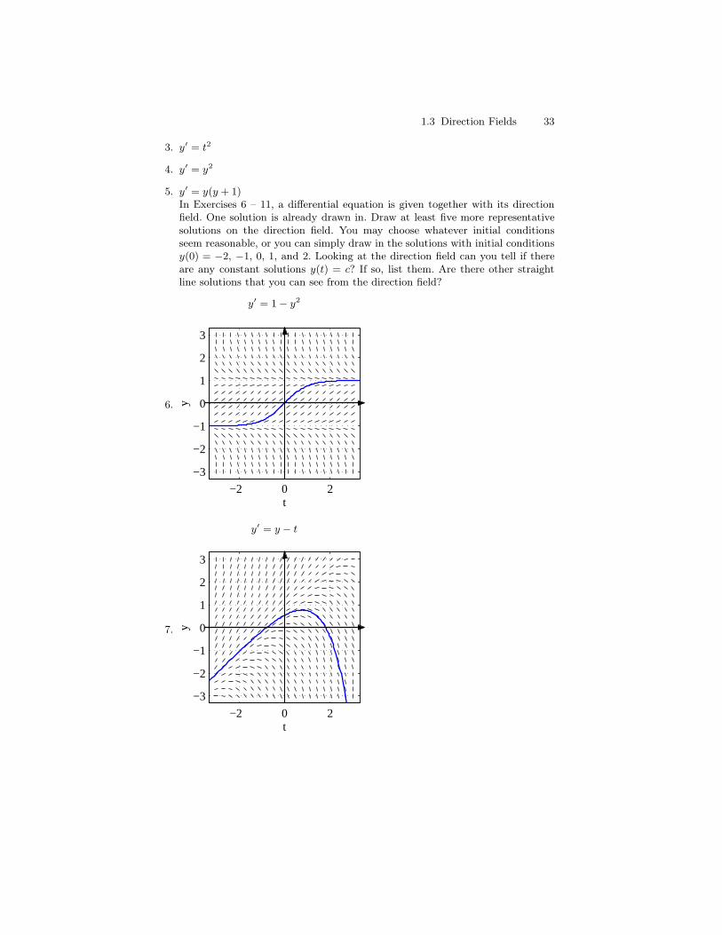
5. y′ = y(y + 1)In Exercises 6 – 11, a differential equation is given together with its directionfield. One solution is already drawn in. Draw at least five more representativesolutions on the direction field. You may choose whatever initial conditionsseem reasonable, or you can simply draw in the solutions with initial conditionsy(0) = −2, −1, 0, 1, and 2. Looking at the direction field can you tell if thereare any constant solutions y(t) = c? If so, list them. Are there other straightline solutions that you can see from the direction field?
6.
y′ = 1 − y2
−2 0 2
−3
−2
−1
0
1
2
3
t
y
7.
y′ = y − t
−2 0 2
−3
−2
−1
0
1
2
3
t
y
34 1 Introduction
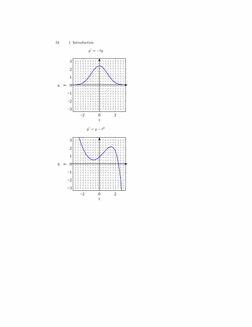
8.
y′ = −ty
−2 0 2
−3
−2
−1
0
1
2
3
t
y
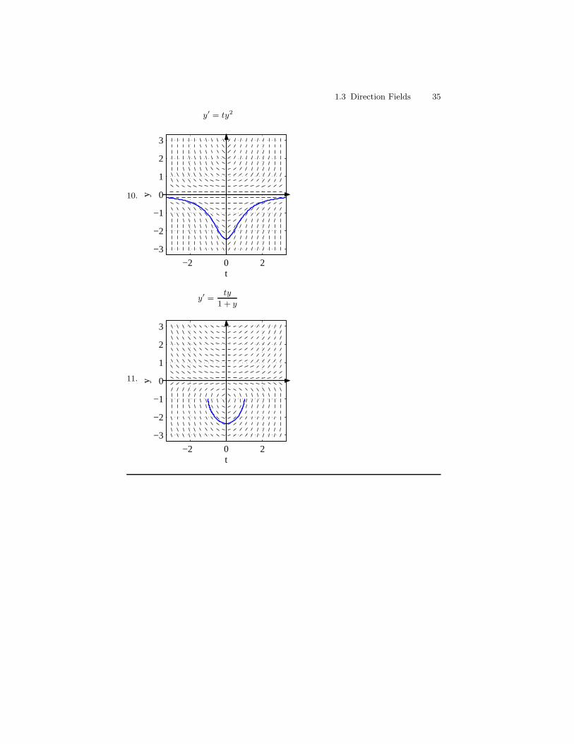
9.
y′ = y − t2
−2 0 2
−3
−2
−1
0
1
2
3
t
y
1.3 Direction Fields 35
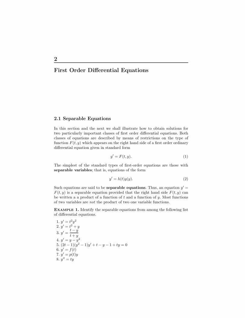
10.
y′ = ty2
−2 0 2
−3
−2
−1
0
1
2
3
t
y
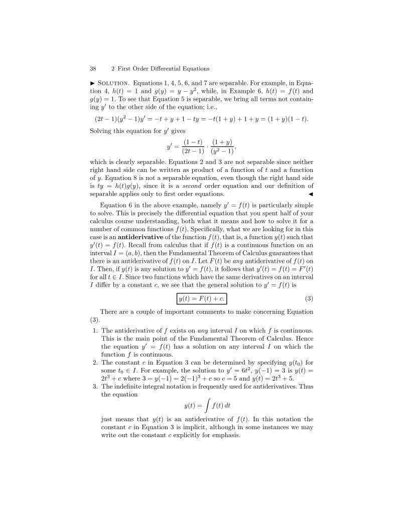
11.
y′ =ty
1 + y
−2 0 2
−3
−2
−1
0
1
2
3
t
y

2
First Order Differential Equations
2.1 Separable Equations
In this section and the next we shall illustrate how to obtain solutions fortwo particularly important classes of first order differential equations. Bothclasses of equations are described by means of restrictions on the type offunction F (t, y) which appears on the right hand side of a first order ordinarydifferential equation given in standard form
y′ = F (t, y). (1)
The simplest of the standard types of first-order equations are those withseparable variables; that is, equations of the form
y′ = h(t)g(y). (2)
Such equations are said to be separable equations. Thus, an equation y′ =F (t, y) is a separable equation provided that the right hand side F (t, y) canbe written a a product of a function of t and a function of y. Most functionsof two variables are not the product of two one variable functions.
Example 1. Identify the separable equations from among the following listof differential equations.
1. y′ = t2y2
2. y′ = t2 + y
3. y′ =t− yt+ y
4. y′ = y − y2
5. (2t− 1)(y2 − 1)y′ + t− y − 1 + ty = 06. y′ = f(t)7. y′ = p(t)y8. y′′ = ty
38 2 First Order Differential Equations
I Solution. Equations 1, 4, 5, 6, and 7 are separable. For example, in Equa-tion 4, h(t) = 1 and g(y) = y − y2, while, in Example 6, h(t) = f(t) andg(y) = 1. To see that Equation 5 is separable, we bring all terms not contain-ing y′ to the other side of the equation; i.e.,
(2t− 1)(y2 − 1)y′ = −t+ y + 1− ty = −t(1 + y) + 1 + y = (1 + y)(1 − t).Solving this equation for y′ gives
y′ =(1− t)(2t− 1)
· (1 + y)
(y2 − 1),
which is clearly separable. Equations 2 and 3 are not separable since neitherright hand side can be written as product of a function of t and a functionof y. Equation 8 is not a separable equation, even though the right hand sideis ty = h(t)g(y), since it is a second order equation and our definition ofseparable applies only to first order equations. J
Equation 6 in the above example, namely y′ = f(t) is particularly simpleto solve. This is precisely the differential equation that you spent half of yourcalculus course understanding, both what it means and how to solve it for anumber of common functions f(t). Specifically, what we are looking for in thiscase is an antiderivative of the function f(t), that is, a function y(t) such thaty′(t) = f(t). Recall from calculus that if f(t) is a continuous function on aninterval I = (a, b), then the Fundamental Theorem of Calculus guarantees thatthere is an antiderivative of f(t) on I. Let F (t) be any antiderivative of f(t) onI. Then, if y(t) is any solution to y′ = f(t), it follows that y′(t) = f(t) = F ′(t)for all t ∈ I. Since two functions which have the same derivatives on an intervalI differ by a constant c, we see that the general solution to y′ = f(t) is
y(t) = F (t) + c. (3)
There are a couple of important comments to make concerning Equation(3).
1. The antiderivative of f exists on any interval I on which f is continuous.This is the main point of the Fundamental Theorem of Calculus. Hencethe equation y′ = f(t) has a solution on any interval I on which thefunction f is continuous.
2. The constant c in Equation 3 can be determined by specifying y(t0) forsome t0 ∈ I. For example, the solution to y′ = 6t2, y(−1) = 3 is y(t) =2t3 + c where 3 = y(−1) = 2(−1)3 + c so c = 5 and y(t) = 2t3 + 5.
3. The indefinite integral notation is frequently used for antiderivatives. Thusthe equation
y(t) =
∫
f(t) dt
just means that y(t) is an antiderivative of f(t). In this notation theconstant c in Equation 3 is implicit, although in some instances we maywrite out the constant c explicitly for emphasis.
2.1 Separable Equations 39
4. The formula y(t) =∫
f(t) dt is valid even if the integral cannot be com-puted in terms of elementary functions. In such a case, you simply leaveyour answer expressed as an integral, and if numerical results are needed,you can use numerical integration. Thus, the only way to describe thesolution to the equation y′ = et2 is to express the answer as
y(t) =
∫
et2 dt.
The indefinite integral notation we have used here has the constant ofintegration implicitly included. One can be more precise by using a definiteintegral notation, as in the Fundamental Theorem of Calculus. With thisnotation,
y(t) =
∫ t
t0
eu2
du + c, y(t0) = c.
We now extend the solution of y′ = f(t) by antiderivatives to the case ofa general separable equation y′ = h(t)g(y), and we provide an algorithm forsolving this equation.
Suppose y(t) is a solution on an interval I of Equation (2), which we writein the form
1
g(y)y′ = h(t),
and let Q(y) be an antiderivative of1
g(y)as a function of y, i.e., Q′(y) =
dQ
dy=
1
g(y)and let H be an antiderivative of h. It follows from the chain rule
thatd
dtQ(y(t)) = Q′(y(t))y′(t) =
1
g(y(t))y′(t) = h(t) = H ′(t).
This equation can be written as
d
dt(Q(y(t))−H(t)) = 0.
Since a function with derivative equal to zero on an interval is a constant, itfollows that the solution y(t) is implicitly given by the formula
Q(y(t)) = H(t) + c. (4)
Conversely, assume that y(t) is any function which satisfies the implicitequation (4). Differentiation of both sides of Equation (4) gives, (again by thechain rule),
h(t) = H ′(t) =d
dt(Q(y(t))) = Q′(y(t))y′(t) =
1
g(y(t))y′(t).
Hence y(t) is a solution of Equation (2).
40 2 First Order Differential Equations
Note that the analysis in the previous two paragraphs is valid as long as
h(t) and q(y) =1
g(y)have antiderivatives. From the Fundamental Theorem
of Calculus, we know that a sufficient condition for this to occur is that h andq are continuous functions, and q will be continuous as long as g is continuousand g(y) 6= 0. We can thus summarize our results in the following theorem.
Theorem 2. Let g be continuous on the interval J = y : c ≤ y ≤ d and leth be continuous on the interval I = t : a ≤ t ≤ b. Let H be an antiderivative
of h on I, and let Q be an antiderivative of1
gon an interval J ′ ⊆ J for which
y0 ∈ J ′ and g(y0) 6= 0. Then y(t) is a solution to the initial value problem
y′ = h(t)g(y); y(t0) = y0 (5)
if and only if y(t) is a solution of the implicit equation
Q(y(t)) = H(t) + c, (6)
where the constant c is chosen so that the initial condition is satisfied. More-over, if y0 is a point for which g(y0) = 0, then the constant function y(t) ≡ y0is a solution of Equation (5).
Proof. The only point not covered in the paragraphs preceding the theoremis the case where g(y0) = 0. But if g(y0) = 0 and y(t) = y0 for all t, then
y′(t) = 0 = h(t)g(y0) = h(t)g(y(t))
for all t. Hence the constant function y(t) = y0 is a solution of Equation (5).ut
We summarize these observations in the following separable equation al-gorithm.
Algorithm 3 (Separable Equation). To solve a separable differential equa-tion, perform the following operations.
1. First put the equation in the form
(I) y′ =dy
dt= h(t)g(y),
if it is not already in that form.2. Then we separate variables in a form convenient for integration, i.e. we
formally write
(II)1
g(y)dy = h(t) dt.
Equation (II) is known as the “differential" form of Equation (I).
2.1 Separable Equations 41
3. Next we integrate both sides of Equation (II) (the left side with respectto y and the right side with respect to t) and introduce a constant c, dueto the fact that antiderivatives coincide up to a constant. This yields
(III)
∫
1
g(y)dy =
∫
h(t) dt+ c.
4. Now evaluate the antiderivatives and solve the resulting implicit equationfor y as a function of t, if you can (this won’t always be possible).
5. Additionally, the numbers y0 with g(y0) = 0 will give constant solutionsy(t) ≡ y0 that will not be seen from the general algorithm. ut
Example 4. Find the solutions of the differential equation y′ =t
y.
I Solution. We first rewrite the equation in the form
(I)dy
dt=t
y
and then in differential form as
(II) y dy = t dt.
Integration of both sides of Equation (II) gives
(III)
∫
y dy =
∫
t dt+ c
or1
2y2 =
1
2t2 + c.
Multiplying by 2 we get y2 = t2 + c, where we write c instead of 2c since twicean arbitrary constant c is still an arbitrary constant. Thus, if a function y(t)satisfies the differential equation yy′ = t, then
y(t) = ±√
t2 + c (∗)
for some constant c ∈ R. On the other hand, since all functions of the form(∗) solve yy′ = t, it follows that the solutions are given by (∗). Figure 2.1shows several of the curves y2 = t2 + c which implicitly define the solutionsof yy′ = t. Note that each of the curves in the upper half plane is the graphof y(t) =
√t2 + c for some c, while each curve in the lower half plane is the
graph of y(t) = −√t2 + c. None of the solutions are defined on the t-axis,
i.e., when y = 0. Notice that each of the solutions is an arm of the hyperbolay2 − t2 = c. J
Example 5. Solve the differential equation y′ = ky where k ∈ R is a con-stant.
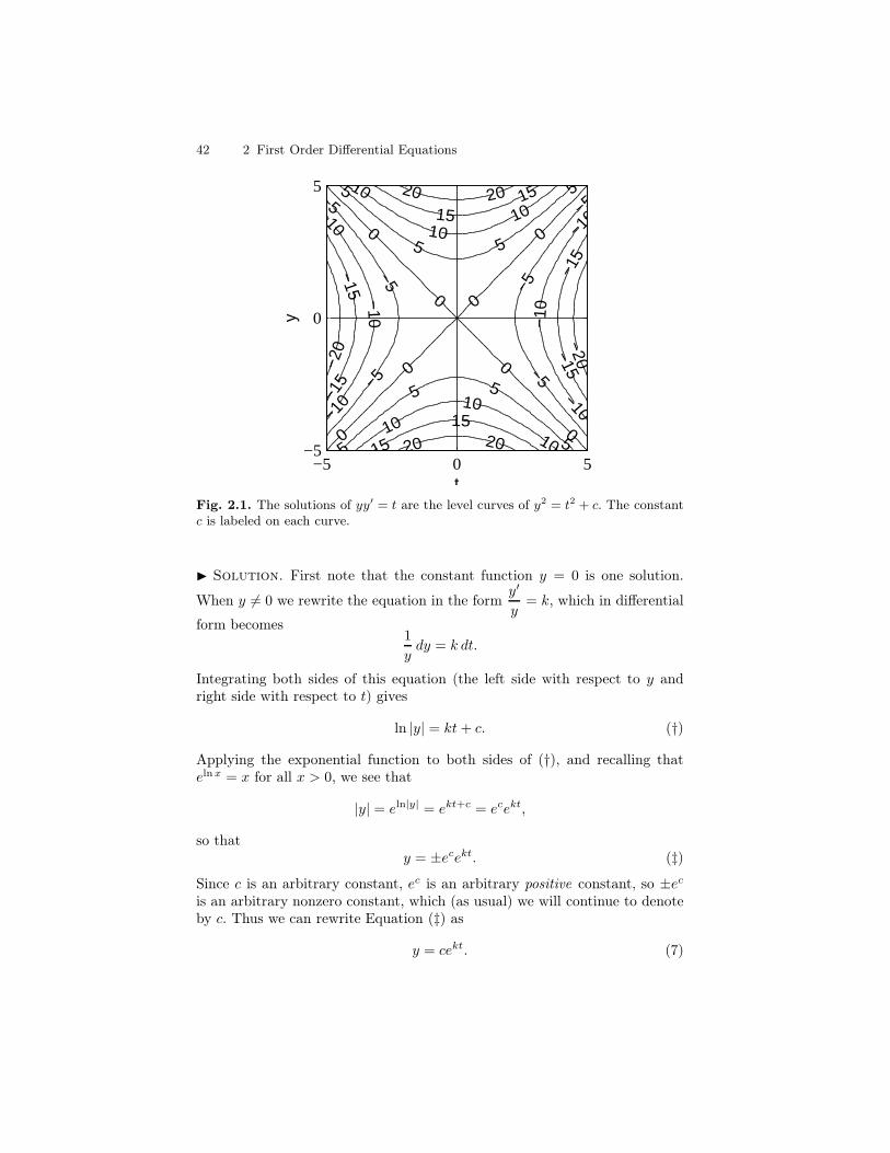
42 2 First Order Differential Equations
−5 0 5−5
0
5
t
y
−20 −20
−15
−15
−15
−15
−10
−10
−10
−10
−10
−10
−5
−5
−5
−5
−5
−5
0
0
0
0
0
0
0
0
5
5 5
5
5
5 5
5
10
1010
1010
10
1515
15
15
20 20
20 20
Fig. 2.1. The solutions of yy′ = t are the level curves of y2 = t2 + c. The constantc is labeled on each curve.
I Solution. First note that the constant function y = 0 is one solution.
When y 6= 0 we rewrite the equation in the formy′
y= k, which in differential
form becomes1
ydy = k dt.
Integrating both sides of this equation (the left side with respect to y andright side with respect to t) gives
ln |y| = kt+ c. (†)
Applying the exponential function to both sides of (†), and recalling thatelnx = x for all x > 0, we see that
|y| = eln|y| = ekt+c = ecekt,
so thaty = ±ecekt. (‡)
Since c is an arbitrary constant, ec is an arbitrary positive constant, so ±ec
is an arbitrary nonzero constant, which (as usual) we will continue to denoteby c. Thus we can rewrite Equation (‡) as
y = cekt. (7)
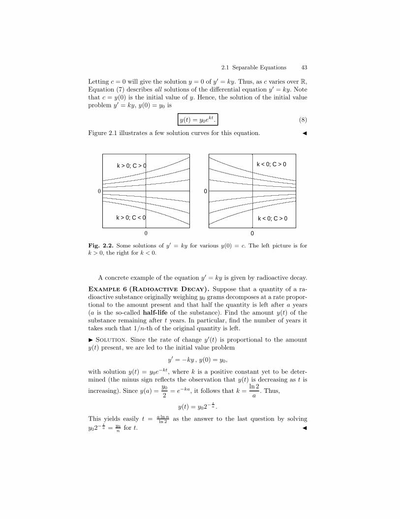
2.1 Separable Equations 43
Letting c = 0 will give the solution y = 0 of y′ = ky. Thus, as c varies over R,Equation (7) describes all solutions of the differential equation y′ = ky. Notethat c = y(0) is the initial value of y. Hence, the solution of the initial valueproblem y′ = ky, y(0) = y0 is
y(t) = y0ekt. (8)
Figure 2.1 illustrates a few solution curves for this equation. J
0
0
k > 0; C > 0
k > 0; C < 0
0
0
k < 0; C > 0
k < 0; C > 0
Fig. 2.2. Some solutions of y′ = ky for various y(0) = c. The left picture is fork > 0, the right for k < 0.
A concrete example of the equation y′ = ky is given by radioactive decay.
Example 6 (Radioactive Decay). Suppose that a quantity of a ra-dioactive substance originally weighing y0 grams decomposes at a rate propor-tional to the amount present and that half the quantity is left after a years(a is the so-called half-life of the substance). Find the amount y(t) of thesubstance remaining after t years. In particular, find the number of years ittakes such that 1/n-th of the original quantity is left.
I Solution. Since the rate of change y′(t) is proportional to the amounty(t) present, we are led to the initial value problem
y′ = −ky , y(0) = y0,
with solution y(t) = y0e−kt, where k is a positive constant yet to be deter-
mined (the minus sign reflects the observation that y(t) is decreasing as t is
increasing). Since y(a) =y02
= e−ka, it follows that k =ln 2
a. Thus,
y(t) = y02− t
a .
This yields easily t = a ln nln 2 as the answer to the last question by solving
y02− t
a = y0
n for t. J
44 2 First Order Differential Equations
Example 7. Solve the differential equation (2t−1)(y2−1)y′+t−y−1+ty =0.
I Solution. To separate the variables in this equation we bring all termsnot containing y′ to the right hand side of the equation, so that
(2t− 1)(y2 − 1)y′ = −t+ y + 1− ty = −t(1 + y) + 1 + y = (1 + y)(1 − t).
This variables can now be separated, yielding
y2 − 1
1 + yy′ =
1− t2t− 1
.
Before further simplification, observe that the constant function y(t) = −1 isa solution of the original problem. If we now consider a solution other thany(t) = −1, the equation can be written in differential form (after expandingthe right hand side in a partial fraction) as
(y − 1) dy =
(
−1
2+
1
2
1
2t− 1
)
dt.
Integrating both sides of the equation gives, 12y
2 − y = − t2 + 1
4 ln |2t− 1|+ c.Solving for y (and renaming the constant several times) we obtain the generalsolution as either y(t) = −1 or
y(t) = 1±√
c− t+1
2ln |2t− 1|.
J
Example 8. Solve the equation p′ = r(m − p)p, known as the Verhulstpopulation equation, where r and m are positive constants.
I Solution. Since
1
(m− p)p =1
m
(
1
p+
1
m− p
)
,
the equation can be written with separated variables in differential form as
1
(m− p)p dp =1
m
(
1
p+
1
m− p
)
dp = r dt,
and the differential form is integrated to give
1
m(ln |p| − ln |m− p|) = rt+ c,
where c is an arbitrary constant of integration. Multiplying bym and renamingmc as c (to denote an arbitrary constant) we get
2.1 Separable Equations 45
ln
∣
∣
∣
∣
p
m− p
∣
∣
∣
∣
= rmt+ c,
and applying the exponential function to both sides of the equation gives∣
∣
∣
∣
p
m− p
∣
∣
∣
∣
= ermt+c = ecermt,
orp
m− p = ±ecermt.
Since c is an arbitrary real constant, it follows that ±ec is an arbitrary realnonzero constant, which we will again denote by c. Thus, we see that p satisfiesthe equation
p
m− p = cermt.
Solving this equation for p, we find that the general solution of the Verhulstpopulation equation is given by
p(t) =cmermt
1 + cermt. (9)
Multiplying the numerator and denominator by e−rmt, we may rewrite Equa-tion (9) in the equivalent form
p(t) =cm
c+ e−rmt. (10)
Some observations concerning this equation:
1. The constant solution p(t) = 0 is obtained by setting c = 0 in Equation(10), even though c = 0 did not occur in our derivation.
2. The constant solution p(t) = m does not occur for any choice of c, so thissolution is an extra one.
3. Note thatlim
t→∞p(t) =
cm
c= m,
independent of c 6= 0. What this means is that if we start with a posi-tive population, then over time, the population will approach a maximum(sustainable) population m.
4. Figure 2.1 shows the solution of the Verhulst population equation y′ =y(3 − y) with initial population y(0) = 1. You can see from the graphthat y(t) approaches the limiting population 3 as t grows. It appears thaty(t) actually equals 3 after some point, but this is not true. It is simplya reflection of the fact that y(t) and 3 are so close together that the lineson a graph cannot distinguish them.
J
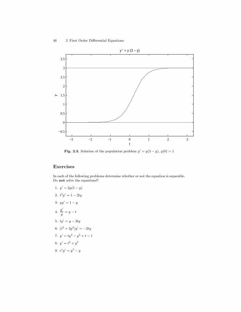
46 2 First Order Differential Equations
−3 −2 −1 0 1 2 3
−0.5
0
0.5
1
1.5
2
2.5
3
3.5
t
yy ’ = y (3 − y)
Fig. 2.3. Solution of the population problem y′ = y(3 − y), y(0) = 1
Exercises
In each of the following problems determine whether or not the equation is separable.Do not solve the equations!!
1. y′ = 2y(5 − y)
2. t2y′ = 1 − 2ty
3. yy′ = 1 − y
4.y′
y= y − t
5. ty′ = y − 2ty
6. (t2 + 3y2)y′ = −2ty
7. y′ = ty2 − y2 + t − 1
8. y′ = t2 + y2
9. ety′ = y3 − y
2.1 Separable Equations 47
Find the general solution of each of the following differential equations. If aninitial condition is given, find the particular solution which satisfies this initial con-dition.
10. yy′ = t, y(2) = −1.
I Solution. The variables are already separated, so integrate both sides of
the equation to get1
2y2 =
1
2t2 + c, which we can rewrite as y2 − t2 = k where
k ∈ R is a constant. Since y(2) = −1, it follows that k = (−1)2 − 22 = −3 sothe solution is given implicitly by the equation y2 − t2 = −3 or we can solveexplicitly to get y = −
√t2 − 3, where the negative square root is used since
y(2) = −1 < 0. J
11. (1 − y2) − tyy′ = 0
I Solution. It is first necessary to separate the variables by rewriting theequation as tyy′ = (1 − y2). This gives an equation
y
1 − y2y′ =
1
t,
or in the language of differentials:
y
1 − y2dy =
1
tdt.
Integrating both sides of this equation gives
−1
2ln |1 − y2| = ln |t| + c.
Multiplying by −2, and taking the exponential of both sides gives an equation|1 − y2| = ±kt−2 where k is a positive constant. By considering an arbitraryconstant (which we will call c), this can be written as an implicit equationt2(1 − y2) = c. J
12. y3y′ = t13. y4y′ = t + 214. y′ = ty2
15. y′ = t2y2
16. y′ + (tan t)y = tan t, −π2
< t < π2
17. y′ = tmyn, where m and n are positive integers, n 6= 1.18. y′ = 4y − y2
19. yy′ = y2 + 120. y′ = y2 + 121. tyy′ + t2 + 1 = 022. y + 1 + (y − 1)(1 + t2)y′ = 023. 2yy′ = et
24. (1 − t)y′ = y2
25. ty − (t + 2)y′ = 0
Solve the following initial value problems:
26. dydt
− y = y2, y(0) = 0.
48 2 First Order Differential Equations
27. y′ = 4ty2, y(1) = 028. dy
dx= xy+2y
x, y(1) = e
29. y′ + 2yt = 0, y(0) = 430. y′ = cot y
t, y(1) = π
4
31. (u2+1)y
dydu
= u, y(0) = 2
2.2 Linear First Order Equations
A linear first order differential equation is an equation of the form
y′ + p(t)y = f(t). (1)
The primary objects of study in the current section are the linear first or-der differential equations where the coefficient function p and the forcingfunction f are continuous functions from an interval I into R. In some exer-cises and in some later sections of the text, we shall have occasion to considerlinear first order differential equations in which the forcing function f is notnecessarily continuous, but for now we restrict ourselves to the case whereboth p and f are continuous. Equation (1) is homogeneous if no forcingfunction is present; i.e., if f(t) = 0 for all t ∈ I; the equation is inhomo-geneous if the forcing function f is not 0, i.e., if f(t) 6= 0 for some t ∈ I.Equation (1) is constant coefficient provided the coefficient function p is aconstant function, i.e., p(t) = p0 ∈ R for all t ∈ I.
Example 1. Consider the following list of first order differential equations.
1. y′ = y − t2. y′ + ty = 03. y′ = f(t)4. y′ + y2 = t5. ty′ + y = t2
6. y′ − 3t y = t4
7. y′ = 7y
All of these equations except for y′ + y2 = t are linear. The presence of they2 term prevents this equation from being linear. The second and the lastequation are homogeneous, while the first, third, fifth and sixth equations areinhomogeneous. The first, third, and last equation are constant coefficient,with p(t) = −1, p(t) = 0, and p(t) = −7 respectively. For the fifth and sixthequations, the interval I on which the coefficient function p(t) and forcingfunction f(t) are continuous can be either (−∞, 0) or (0,∞). In both of thesecases, p(t) = 1/t or p(t) = −3/t fails to be continuous at t = 0. For thefirst, second, and last equations, the interval I is all of R, while for the thirdequation I is any interval on which the forcing function f(t) is continuous.Note that only the second, third and last equations are separable. ut
2.2 Linear First Order Equations 49
Remark 2. Notice that Equation (1), which is the traditional way to expressa linear first order differential equation, is not in the standard form of Equation(5). In standard form, Equation (1) becomes
y′ = −p(t)y + f(t), (2)
so that the function F (t, y) of Equation (5) is F (t, y) = −p(t)y + f(t). Thestandard form of the equation is useful for expressing the hypotheses whichwill be used in the existence and uniqueness results of Section 2.3, while theform given by Equation (1) is particularly useful for describing the solutionalgorithm to be presented in this section. From Equation (2) one sees thatif a first order linear equation is homogeneous (i.e. f(t) = 0 for all t), thenthe equation is separable (the right hand side is −p(t)y) and the technique ofthe previous section applies, while if neither p(t) nor f(t) is the zero function,then Equation (2) is not separable, and hence the technique of the previoussection is not applicable.
We will describe an algorithm for finding all solutions to the linear differ-ential equation
y′ + p(t)y = f(t)
which is based on first knowing how to solve homogeneous linear equations(i.e., f(t) = 0 for all t). But, as we observed above, the homogeneous linearequation is separable, and hence we know how to solve it.
Homogeneous Linear Equation: y′ = h(t)y
Since the equation y′ = h(t)y is separable, we first separate the variables andwrite the equation in differential form:
1
ydy = h(t) dt. (∗)
If H(t) =∫
h(t) dt is any antiderivative of h(t), then integration of both sidesof Equation (∗) gives
ln |y| = H(t) + c
where c is a constant of integration. Applying the exponential function toboth sides of this equation gives
|y| = eln|y| = eH(t)+c = eceH(t).
Since c is an arbitrary constant, ec is an arbitrary positive constant. Theny = ± |y| = ±eceH(t) where ±ec will be an arbitrary nonzero constant, which,as usual we will continue to denote by c. Since the constant function y(t) = 0is also a solution to (∗), and we conclude that, if H(t) =
∫
h(t) dt, then thegeneral solution to y′ = h(t)y is
50 2 First Order Differential Equations
y(t) = ceH(t) (3)
where c denotes any real number.
Example 3. Solve the equation y′ =3
ty on the interval (0,∞).
I Solution. In this case h(t) =3
tso that an antiderivative on the interval
(0,∞) is
H(t) =
∫
3
tdt = 3 ln t = ln(t3).
Hence then general solution of y′ =3
ty is
y(t) = ceH(t) = celn(t3) = ct3.
J
We can now use the homogeneous case to transform an arbitrary firstorder linear differential equation into an equation which can be solved byantidifferentiation. What results is an algorithmic procedure for determiningall solutions to the linear first order equation
y′ + p(t)y = f(t). (†)
The key observation is that the left hand side of this equation looks almostlike the derivative of a product. Recall that if z(t) = µ(t)y(t), then
z′(t) = µ(t)y′(t) + µ′(t)y(t). (‡)
Comparing this with Equation (†), we see that what is missing is the coefficientµ(t) in front of y′(t). If we multiply Equation (†) by µ(t), we get an equation
µ(t)y′(t) + µ(t)p(t)y(t) = µ(t)f(t).
The left hand side of this equation agrees with the right hand side of (‡)provided the multiplier function µ(t) is chosen so that the coefficients of y(t)agree in both equations. That is, choose µ(t), if possible, so that
µ′(t) = p(t)µ(t).
But this is a homogeneous linear first order differential equation, so by Equa-tion (3) we may take µ(t) = eP (t) where P (t) is any antiderivative of p(t) onthe given interval I. The function µ(t) is known an an integrating factorfor the equation y′ + p(t)y = f(t), since after multiplication by µ(t), the lefthand side becomes a derivative (µ(t)y)′ and the equation itself becomes
(µ(t)y)′ = µ(t)f(t),
2.2 Linear First Order Equations 51
which is an equation that can be solved by integration. Recalling that∫
g′(t) dt = g(t) + c, we see that integrating the above equation gives
µ(t)y(t) =
∫
µ(t)f(t) dt.
Putting together all of our steps, we arrive at the following theorem de-scribing all the solutions of a first order linear differential equation. The proofis nothing more than an explicit codification of the steps delineated above intoan algorithm to follow.
Theorem 4. Let p(t), f(t) be continuous functions on an interval I. Afunction y(t) is a solution of of the first order linear differential equationy′ + p(t)y = f(t) (Equation (1)) on I if and only if
y(t) = ce−P (t) + e−P (t)
∫
eP (t)f(t) dt (4)
for all t ∈ I, where c ∈ R, and P (t) is some antiderivative of p(t) on theinterval I.
Proof. Let y(t) = ce−P (t) + e−P (t)∫
eP (t)f(t) dt. Since P ′(t) = p(t) andd
dt
∫
eP (t)f(t) dt = eP (t)f(t) (this is what it means to be an antiderivative
of eP (t)f(t)) we obtain
y′(t) = −cp(t)e−P (t) − p(t)e−P (t)
∫
eP (t)f(t) dt+ e−P (t)eP (t)f(t)
= −p(t)(
ce−P (t) + e−P (t)
∫
eP (t)f(t) dt
)
+ f(t)
= −p(t)y(t) + f(t)
for all t ∈ I. This shows that every function of the form (4) is a solution ofEquation (1). Next we show that any solution of Equation (1) has a representa-tion in the form of Equation (4). This is essentially what we have already donein the paragraphs prior to the statement of the theorem. What we shall donow is summarize the steps to be taken to implement this algorithm. Let y(t)be a solution of Equation (1) on the interval I. Then we perform the follow-ing step-by-step procedure, which will be crucial when dealing with concreteexamples.
Algorithm 5 (Solution of First Order Linear Equations). Follow thefollowing procedure to put any solution y(t) of Equation (1) into the formgiven by Equation (4).
1. Compute an antiderivative P (t) =∫
p(t) dt and multiply the equationy′ + p(t)y = f(t) by the integrating factor µ(t) = eP (t). This yields
(I) eP (t)y′(t) + p(t)eP (t)y(t) = eP (t)f(t).
52 2 First Order Differential Equations
2. The function µ(t) = eP (t) is an integrating factor (see the paragraphsprior to the theorem) which means that the left hand side of Equation (I)is a perfect derivative, namely (µ(t)y(t))′. Hence, Equation (I) becomes
(II)d
dt(µ(t)y(t)) = eP (t)f(t).
3. Now we take an antiderivative of both sides and observe that they mustcoincide up to a constant c ∈ R. This yields
(III) eP (t)y(t) =
∫
eP (t)f(t) dt+ c.
4. Finally, multiply by µ(t)−1 = e−P (t) to get that y(t) is of the form
(IV) y(t) = ce−P (t) + e−P (t)
∫
eP (t)f(t) dt.
This shows that any solution of Equation (1) is of the form given byEquation (4), and moreover, the steps of Algorithm 5 tell one precisely howto find this form. ut
ut
Remark 6. You should not memorize formula (4). What you should remem-ber instead is the sequence of steps in Algorithm 5, and apply these steps toeach concretely presented linear first order differential equation (given in theform of Equation (1)). To summarize the algorithm in words:
1. Find an integrating factor µ(t).2. Multiply the equation by µ(t), insuring that the left hand side of the
equation is a perfect derivative.3. Integrate both sides of the resulting equation.4. Divide by µ(t) to give the solution y(t).
Example 7. Find all solutions of the differential equation t2y′ + ty = 1 onthe interval (0,∞).
I Solution. Clearly, you could bring the equation into the standard formof Equation (1), that is
y′ +1
ty =
1
t2,
identify p(t) =1
tand f(t) =
1
t2, compute an antiderivative P (t) = ln(t) of
p(t) on the interval (0,∞), plug everything into formula (4), and then computethe resulting integral. This is a completely valid procedure if you are good inmemorizing formulas. Since we are not good at memorization, we prefer gothrough the steps of Algorithm 5 explicitly.
First bring the differential equation into the standard form
2.2 Linear First Order Equations 53
y′ +1
ty =
1
t2.
Then compute an antiderivative P (t) of the function in front of y and multiplythe equation by the integrating factor µ(t) = eP (t). In our example, we takeP (t) = ln(t) and multiply the equation by µ(t) = eP (t) = eln(t) = t (we couldalso take P (t) = ln(t)+ c for any constant c, but the computations are easiestif we set the constant equal to zero). This yields
(I) ty′ + y =1
t.
Next observe that the left side of this equality is equal tod
dt(ty) (see Step 2
of Algorithm 5). Thus,
(II)d
dt(ty) =
1
t.
Now take antiderivatives of both sides and observe that they must coincideup to a constant c ∈ R. Thus,
(III) ty = ln(t) + c, or
(IV) y(t) = c1
t+
1
tln(t).
Observe that yh(t) = c1
t(c ∈ R) is the general solution of the homogeneous
equation t2y′+ty = 0, and that yp(t) =1
tln(t) is a particular solution of t2y′+
ty = 1. Thus, all solutions are given by y(t) = yh(t) + yp(t). As the followingremark shows, this holds for all linear first order differential equations. J
Remark 8. Analyzing the general solution y(t) = ce−P (t)+e−P (t)∫
eP (s)f(s) ds,we see that this general solution is the sum of two parts. Namely, yh(t) =ce−P (t) which is the general solution of the homogeneous problem
y′ + p(t)y = 0,
and yp(t) = e−P (t)∫
eP (s)f(s) ds which is a particular, i.e., a single, solutionof the inhomogeneous problem
y′ + p(t)y = f(t).
The homogeneous equation y′ + p(t)y = 0 is known as the associated ho-mogeneous equation of the linear equation y′ + p(t)y = f(t). That is, theright hand side of the general linear equation is replaced by 0 to get the asso-ciated homogeneous equation. The relationship between the general solution
54 2 First Order Differential Equations
yg(t) of y′ + p(t)y = f(t), a particular solution yp(t) of this equation, and thegeneral solution yh(t) of the associated homogeneous equation y′ + p(t)y = 0,is usually expressed as
yg(t) = yh(t) + yp(t). (5)
What this means is that every solution to y′ + p(t)y = f(t) can be obtainedby starting with a single solution yp(t) and adding to that an appropriatesolution of y′ + p(t)y = 0. The key observation is the following. Suppose thaty1(t) and y2(t) are any two solutions of y′ + p(t)y = f(t). Then
(y2 − y1)′(t) + p(t)(y2 − y1)(t) = (y′2(t) + p(t)y2(t)) − (y′1(t) + p(t)y1(t))
= f(t)− f(t)
= 0,
so that y2(t) − y1(t) is a solution of the associated homogeneous equationy′ + p(t)y = 0, and y2(t) = y1(t) + (y2(t)− y1(t)). Therefore, given a solutiony1(t) of y′ + p(t)y = f(t), any other solution y2(t) is obtained from y1(t) byadding a solution (specifically y2(t) − y1(t)) of the associated homogeneousequation y′ + p(t)y = 0.
This observation is a general property of solutions of linear equations,whether they are differential equations of first order (as above), differentialequations of higher order (to be studied in Chapter 6), linear algebraic equa-tions, or linear equations L(y) = f in any vector space, which is the math-ematical concept created to handle the features common to problems of lin-earity.. Thus, the general solution set S = yg of any linear equation L(y) = f
is of the formyg = S = L−1(0) + yp = yh + yp,
where L(yp) = f and L−1(0) = yh = y : L(y) = 0.
Corollary 9. Let p(t), f(t) be continuous on an interval I, t0 ∈ I, and y0 ∈R. Then the unique solution of the initial value problem
y′ + p(t)y = f(t), y(t0) = y0 (6)
is given by
y(t) = y0e−P (t) + e−P (t)
∫ t
t0
eP (u)f(u) du, (7)
where P (t) =∫ t
t0p(u) du.
Proof. Since P (t) is an antiderivative of p(t), we see that y(t) has the form ofEquation (4), and hence Theorem 4 guarantees that y(t) is a solution of thelinear first order equation y′+p(t)y = f(t). Moreover, P (t0) =
∫ t0t0p(u) du = 0,
and
y(t0) = y0e−P (t0) + e−P (t0)
∫ t0
t0
eP (u)f(u) du = y0,
2.2 Linear First Order Equations 55
so that y(t) is a solution of the initial value problem (6). Suppose that y1(t)is any other solution of Equation (6). Then y2(t) := y(t)− y1(t) is a solutionof the associated homogeneous equation
y′ + p(t)y = 0, y(t0) = 0.
It follows from Equation (3) that y2(t) = ce−P (t) for some constant c ∈ R andan antiderivative P (t) of p(t). Since y2(t0) = 0 and e−P (t0) 6= 0, it follows thatc = 0. Thus, y(t)−y1(t) = y2(t) = 0 for all t ∈ I. This shows that y1(t) = y(t)for all t ∈ I, and hence y(t) is the only solution of Equation (6). ut
Example 10. Find the solution of the initial value problem y′ = −ty +t, y(2) = 7 on R.
I Solution. Again, you could bring the differential equation into the stan-dard form
y′ + ty = t,
identify p(t) = t and f(t) = t, compute the antiderivative
P (t) =
∫ t
2
u du =t2
2− 2
of p(t), plug everything into the formula (4), and then compute the integralin (7) to get
y(t) = y0e−P (t) + e−P (t)
∫ t
t0
eP (u)f(u) du
= 7e−t2
2 +2 + e−t2
2 +2
∫ t
2
ueu2
2 −2 du.
However, we again prefer to follow the steps of the algorithm. First weproceed as in Example 7 and find the general solution of
y′ + ty = t.
To do so we multiply the equation by the integrating factor et2/2 and obtain
et2/2y′ + tet2/2y = tet2/2.
Since the left side is the derivative of et2/2y, this reduces to
d
dt
(
et2/2y)
= tet2/2.
Since et2/2 is the antiderivative of tet2/2, it follows that
et2/2y(t) = et2/2 + c, or y(t) = ce−t2/2 + 1.
56 2 First Order Differential Equations
Finally, we determine the constant c such that y(2) = 7. This yields 7 =ce−2 + 1 or c = 6e2. Thus, the solution is given by
y(t) = 6e−t2
2 +2 + 1.
J
Corollary 11. Let f(t) be a continuous function on an interval I and p ∈ R.Then all solution of the first order, inhomogeneous, linear, constant coeffi-cient differential equation
y′ + py = f(t)
are given by
y(t) = ce−pt +
∫
e−p(t−u)f(u) du.
Moreover, for any t0, y0 ∈ R, the unique solution of the initial value problem
y′ + py = f(t), y(t0) = y0
is given by
y(t) = y0e−p(t−t0) +
∫ t
t0
e−p(t−u)f(u) du.
Proof. The statements follow immediately from Corollary 9. ut
Example 12. Find the solution of the initial value problem y′ = −y +4, y(0) = 8 on R.
I Solution. We write the equation as y′ + y = 4 and apply Corollary 11.This yields
y(t) = 8e−t+
∫ t
0
4e−(t−u) ds = 8e−t+4e−t
∫ t
0
eu du = 8e−t+4e−t[
et − 1]
= 4e−t+4.
J
Example 13. Find the solution of the initial value problem y′ + y =1
1−t , y(0) = 0 on the interval (−∞, 1).
I Solution. By Corollary 11, y(t) = e−t∫ t
01
1−ueu du. Since the function
1
1− ueu is not integrable in closed form on the interval (−∞, 1), we might be
tempted to stop at this point and say that we have solved the equation. Whilethis is a legitimate statement, the present representation of the solution is oflittle practical use and a further detailed study is necessary if you are “really”interested in the solution. Any further analysis (numerical calculations, qual-itative analysis, etc.) would be based on what type of information you areattempting to ascertain about the solution. J
2.2 Linear First Order Equations 57
We can use our analysis of first order linear differential equations to solvethe mixing problem set up in Example 5. For convenience we restate theproblem.
Example 14. Consider a tank that contains 2000 gallons of water in which10 lbs of salt are dissolved. Suppose that a water-salt mixture containing0.1 lb/gal enters the tank at a rate of 2 gal/min, and assume that the well-stirred mixture flows from the tank at the same rate of 2 gal/min. Find theamount y(t) of salt (expressed in pounds) which is present in the tank at alltimes t measured in minutes.
I Solution. In Example 5, it was determined that y(t) satisfies the initialvalue problem
y′ + (0.001)y = 0.2, y(0) = 10. (8)
This equation has an integrating factor µ(t) = e(0.001)t, so multiplying theequation by µ(t) gives
(
e(0.001)ty)′
= (0.2)e(0.001)t.
Integration of this equation gives e(0.001)ty = 200e(0.001)t + c, or after solvingfor y,
y(t) = 200 + ce−(0.001)t.
Setting t = 0 gives 10 = y(0) = 200+ c so that c = −190 and the final answeris
y(t) = 200− 190e−(0.001)t.
J
Next we consider a numerical example of the general mixing problem con-sidered in Example 6
Example 15. A large tank contains 100 gal of brine in which 50 lb of saltis dissolved. Brine containing 2 lb of salt per gallon runs into the tank at therate of 6 gal/min. The mixture, which is kept uniform by stirring, runs out ofthe tank at the rate of 4 gal/min. Find the amount of salt in the tank at theend of t minutes.
I Solution. Let y(t) denote the number of pounds of salt in the tank aftert minutes; note that the tank will contain 100 + (6 − 4)t gallons of brine atthis time. The concentration (number of pounds per gallon) will then be
y(t)
100 + 2tlb/gal.
Instead of trying to find the amount (in pounds) of salt y(t) at time t directly,we will follow the analysis of Example 6 and determine the rate of change
58 2 First Order Differential Equations
of y(t), i.e., y′(t). But the the change of y(t) at time t is governed by theprinciple
y′(t) = input rate − output rate,
where all three rates have to be measured in the same unit, which we take tobe lb/min. Thus,
input rate = 2 lb/gal × 6 gal/min = 12 lb/min,
output rate =y(t)
100 + 2tlb/gal × 4 gal/min =
4y(t)
100 + 2tlb/min.
This yields the initial value problem
y′(t) = 12− 4y(t)
100 + 2t, y(0) = 50
which can be solved as in the previous examples. The solution is seen to be
y(t) = 2(100 + 2t)− 15(105)
(100 + 2t)2.
After 50 min, for example, there will be 362.5 lb of salt in the tank and 200 galof brine. J
Exercises
Find the general solution of the given differential equation. If an initial conditionis given, find the particular solution which satisfies this initial condition. Examples3, 7, and 10 are relevant examples to review, and detailed solutions of a few of theexercises will be provided for you to study.
1. y′(t) + 3y(t) = et, y(0) = −2.
I Solution. This equation is already in standard form (Equation (3.1.1)) withp(t) = 3. An antiderivative of p(t) is P (t) =
3 dt = 3t. If we multiply the
differential equation y′(t) + 3y(t) = et by P (t), we get the equation
e3ty′(t) + 3e3ty(t) = e4t,
and the left hand side of this equation is a perfect derivative, namely,d
dt(e3ty(t)).
Thus,d
dt(e3ty(t)) = e4t.
Now take antiderivatives of both sides and observe that they must coincide upto a constant c ∈ R. This gives
e3ty(t) =1
4e4t + c.
2.2 Linear First Order Equations 59
Now, multiplying by e−3t gives
y(t) =1
4et + ce−3t (∗)
for the general solution of the equation y′(t)+3y(t) = et. To choose the constantc to satisfy the initial condition y(0) = −2, substitute t = 0 into Equation (*)
to get −2 = y(0) =1
4+ c (remember that e0 = 1). Hence c = −9
4, and the
solution of the initial value problem is
y(t) =1
4et − 9
4e−3t.
J
2. (cos t)y′(t) + (sin t)y(t) = 1, y(0) = 5
I Solution. Divide the equation by cos t to put it in the standard form
y′(t) + (tan t)y(t) = sec t.
In this case p(t) = tan t and an antiderivative is P (t) =
tan t dt = ln(sec t). (Wedo not need | sec t| since we are working near t = 0 where sec t > 0.) Now multi-ply the differential equation y′(t) + (tan t)y(t) = sec t by eP (t) = eln sec t = sec tto get (sec t)y′(t) + (sec t tan t)y(t) = sec2 t, the left hand side of which is a
perfect derivative, namelyd
dt((sec t)y(t)). Thus
d
dt((sec t)y(t)) = sec2 t
and taking antiderivatives of both sides gives
(sec t)y(t) = tan t + c
where c ∈ R is a constant. Now multiply by cos t to eliminate the sec t in frontof y(t), and we get
y(t) = sin t + c cos t
for the general solution of the equation, and letting t = 0 gives 5 = y(0) =sin 0 + c cos 0 = c so that the solution of the initial value problem is
y(t) = sin t + 5 cos t.
J
3. y′ − 2y = e2t, y(0) = 4
4. y′ − 2y = e−2t, y(0) = 4
5. ty′ + y = et, y(1) = 0
6. ty′ + y = e2t, y(1) = 0.
60 2 First Order Differential Equations
7. y′ = (tan t)y + cos t
8. y′ + ty = 1, y(0) = 1.
9. ty′ + my = t ln(t), where m is a constant.
10. y′ = − yt
+ cos(t2)
11. t(t + 1)y′ = 2 + y.
12. y′ + ay = b, where a and b are constants.
13. y′ + y cos t = cos t, y(0) = 1
14. y′ − 2
t + 1y = (t + 1)2
15. y′ − 2
ty =
t + 1
t, y(1) = −3
16. y′ + ay = e−at, where a is a constant.
17. y′ + ay = ebt, where a and b are constants and b 6= −a.
18. y′ + ay = tne−at, where a is a constant.
19. y′ = y tan t + sec t
20. ty′ + 2y ln t = 4 ln t
21. y′ − n
ty = ettn
22. y′ − y = te2t, y(0) = a
23. ty′ + 3y = t2, y(−1) = 2
24. t2y′ + 2ty = 1, y(2) = a
Before attempting the following exercises, you may find it helpful to review theexamples in Section 1.1 related to mixing problems.
25. A tank contains 10 gal of brine in which 2 lb of salt are dissolved. Brine con-taining 1 lb of salt per gallon flows into the tank at the rate of 3 gal/min, andthe stirred mixture is drained off the tank at the rate of 4 gal/min. Find theamount y(t) of salt in the tank at any time t.
26. A 100 gal tank initially contains 10 gal of fresh water. At time t = 0, a brinesolution containing .5 lb of salt per gallon is poured into the tank at the rate of 4gal/min while the well-stirred mixture leaves the tank at the rate of 2 gal/min.a) Find the time T it takes for the tank to overflow.b) Find the amount of salt in the tank at time T .c) If y(t) denotes the amount of salt present at time t, what is limt→∞ y(t)?
27. A tank contains 100 gal of brine made by dissolving 80 lb of salt in water. Purewater runs into the tank at the rate of 4 gal/min, and the mixture, which iskept uniform by stirring, runs out at the same rate. Find the amount of salt inthe tank at any time t. Find the concentration of salt in the tank at any time t.
2.3 Existence and Uniqueness 61
28. For this problem, our tank will be a lake and the brine solution will be pollutedwater entering the lake. Thus assume that we have a lake with volume V whichis fed by a polluted river. Assume that the rate of water flowing into the lakeand the rate of water flowing out of the lake are equal. Call this rate r, let c bethe concentration of pollutant in the river as it flows into the lake, and assumeperfect mixing of the pollutant in the lake (this is, of course, a very unrealisticassumption).a) Write down and solve a differential equation for the amount P (t) of pol-
lutant in the lake at time t and determine the limiting concentration ofpollutant in the lake as t → ∞.
b) At time t = 0, the river is cleaned up, so no more pollutant flows into thelake. Find expressions for how long it will take for the pollution in the laketo be reduced to (i) 1/2 (ii) 1/10 of the value it had at the time of theclean-up.
c) Assuming that Lake Erie has a volume V of 460 km3 and an inflow-outflowrate of r = 175 km3/year, give numerical values for the times found in Part(b). Answer the same question for Lake Ontario, where it is assumed thatV = 1640 km3 and r = 209 km3/year.
29. A 30 liter container initially contains 10 liters of pure water. A brine solutioncontaining 20 grams salt per liter flows into the container at a rate of 4 litersper minute. The well stirred mixture is pumped out of the container at a rateof 2 liters per minute.
a) How long does it take the container to overflow?b) How much salt is in the tank at the moment the tank begins to overflow?
30. A tank holds 10 liters of pure water. A brine solution is poured into the tank ata rate of 1 liter per minute and kept well stirred. The mixture leaves the tankat the same rate. If the brine solution has a concentration of 1 kg salt per literwhat will the concentration be in the tank after 10 minutes.
2.3 Existence and Uniqueness
Unfortunately, only a few simple types of differential equations can be solvedexplicitly in terms of well known elementary functions. In this section we willdescribe the method of successive approximations, which provides one ofthe many possible lines of attack for approximating solutions for arbitrarydifferential equations. This method, which is quite different from what moststudents have previously encountered, is the primary idea behind one of themain theoretical results concerning existence and uniqueness of solutions ofthe initial value problem
(∗) y′ = F (t, y), y(t0) = y0,
where F (t, y) is a continuous function of (t, y) in the rectangle
R := (t, y) : a ≤ t ≤ b , c ≤ y ≤ d
62 2 First Order Differential Equations
and (t0, y0) ∈ R. The key to the method of successive approximations is thefact that a continuously differentiable function y(t) is a solution of (∗) if andonly if it is a solution of the integral equation
(∗∗) y(t) = y0 +
∫ t
t0
F (u, y(u)) du.
To see the equivalence of the initial value problem (∗) and the integralequation (∗∗), we first integrate (∗) from t0 to t and obtain (∗∗). Con-versely, if y(t) is a continuously differentiable solution of (∗∗), then y(t0) =
y0 +∫ t0
t0F (u, y(u)) du = y0. Moreover, since y(t) is a continuous function in t
and F (t, y) is a continuous function of (t, y), it follows that g(t) := F (t, y(t))is a continuous function of t. Thus, by the Fundamental Theorem of Calculus,
y′(t) =d
dt
(
y0 +
∫ t
t0
F (u, y(u)) du
)
=d
dt
(
y0 +
∫ t
t0
g(u) du
)
= g(t) = F (t, y(t)),
which is what it means to be a solution of (∗).To solve the integral equation (∗∗), mathematicians have developed a va-
riety of so-called “fixed point theorems”, each of which leads to an existenceand/or uniqueness result for solutions to the integral equation. One of theoldest and most widely used existence and uniqueness theorems is due toÉmile Picard (1856-1941). Assuming that the function F (t, y) is sufficiently“nice”, he first employed the method of successive approximations to provethe existence and uniqueness of solutions of (∗∗). The method of successiveapproximations is an iterative procedure which begins with a crude approx-imation of a solution and improves it using a step by step procedure whichbrings us as close as we please to an exact and unique solution of (∗∗). Thealgorithmic procedure follows.
Algorithm 1 (Picard Approximation). Perform the following sequenceof steps to produce an approximate solution to the integral equation (∗∗), andhence to initial value problem (∗).(i) A rough initial approximation to a solution of (∗∗) is given by the constant
functiony0(t) := y0.
(ii) Insert this initial approximation into the right hand side of equation (∗∗)and obtain the first approximation
y1(t) := y0 +
∫ t
t0
F (u, y0(u)) du.
(iii)The next step is to generate the second approximation in the same way;i.e.,
y2(t) := y0 +
∫ t
t0
F (u, y1(u)) du.
2.3 Existence and Uniqueness 63
(iv)At the n-th stage of the process we have
yn(t) := y0 +
∫ t
t0
F (u, yn−1(u)) du,
which is defined by substituting the previous approximation yn−1(t) intothe right hand side of (∗∗).
It is one of Picard’s great contributions to mathematics that he showed thatthe functions yn(t) converge to a unique, continuously differentiable solutiony(t) of (∗∗) (and thus of (∗)) if the function F (t, y) and its partial derivative
Fy(t, y) :=∂
∂yF (t, y) are continuous functions of (t, y) on the rectangle R.
Theorem 2 (Picard’s Existence and Uniqueness Theorem). 1 LetF (t, y) and Fy(t, y) be continuous functions of (t, y) on a rectangle
R = (t, y) : a ≤ t ≤ b , c ≤ y ≤ d .
If (t0, y0) is an interior point of R, then there exists a unique solution y(t) of
(∗) y′ = F (t, y) , y(t0) = y0,
on some interval [a′, b′] with t0 ∈ [a′, b′] ⊂ [a, b]. Moreover, the successiveapproximations y0(t) := y0,
yn(t) := y0 +
∫ t
t0
F (u, yn−1(u)) du,
computed by Algorithm 1 converge towards y(t) on the interval [a′, b′]. Thatis, for all ε > 0 there exists n0 such that the maximal distance between thegraph of the functions yn(t) and the graph of y(t) (for t ∈ [a′, b′]) is less thanε for all n ≥ n0.
If one only assumes that the function F (t, y) is continuous on the rectangleR, but makes no assumptions about Fy(t, y), then Guiseppe Peano (1858-1932) showed that the initial value problem (∗) still has a solution on someinterval I with t0 ∈ I ⊂ [a, b]. This statement is known as Peano’s ExistenceTheorem.2 However, in this case the solutions are not necessarily unique(see Example 5 below). Theorem 2 is called a local existence and uniquenesstheorem because it guarantees the existence of a unique solution in someinterval I ⊂ [a, b]. In contrast, the following important variant of Picard’stheorem yields a unique solution on the whole interval [a, b].
1A proof of this theorem can be found in G.F. Simmons’ book Differential Equa-
tions with Applications and Historical Notes, 2nd edition McGraw-Hill, 1991.2For a proof see, for example, A.N. Kolmogorov and S.V. Fomin, Introductory
Real Analysis, Chapter 3, Section 11, Dover 1975.
64 2 First Order Differential Equations
Theorem 3. Let F (t, y) be a continuous function of (t, y) that satisfies aLipschitz condition on a strip S = (t, y) : a ≤ t ≤ b , −∞ < y < ∞. Thatis, assume that
|F (t, y1)− F (t, y2)| ≤ K|y1 − y2|for some constant K > 0. If (t0, y0) is an interior point of S, then there existsa unique solution of
(∗) y′ = F (t, y) , y(t0) = y0,
on the interval [a, b].
Example 4. Let us consider the Riccati equation y′ = y2−t. Here, F (t, y) =y2−t and Fy(t, y) = 2y are continuous on all of R2. Thus, by Picard’s Theorem2, the initial value problem
(∗) y′ = y2 − t , y(0) = 0
has a unique solution on some (finite or infinite) interval I containing 0. Thedirection field for y′ = y2 − t (see Section 1.3, Example 3) suggests that themaximal interval Imax on which the solution exists should be of the formImax = (a,∞) for some −∞ ≤ a < −1. Observe that we can not applyTheorem 3 since
|F (t, y1)− F (t, y2)| =∣
∣(y21 − t)− (y2
2 − t)∣
∣ = |y21 − y2
2 | = |y1 + y2||y1 − y2|
can not be bounded by K|y1−y2| for some constant K > 0 because this wouldimply that |y1 + y2| ≤ K for all −∞ < y1, y2 < ∞. Thus, without furtheranalysis of the problem, we have no precise knowledge about the maximaldomain of the solution; i.e., we do not know if and where the solution will“blow up”.
Next we show how Picard’s method of successive approximations works inthis example. To use this method we rewrite the initial value problem (∗) asan integral equation; i.e., we consider
(∗∗) y(t) =
∫ t
0
(y(u)2 − u) du.
We start with our initial approximation y0(t) = 0, plug it into (∗∗) and obtainour first approximation
y1(t) =
∫ t
0
(y0(u)2 − u) du = −
∫ t
0
u du = −1
2t2.
The second iteration yields
y2(t) =
∫ t
0
(y1(u)2 − u) du =
∫ t
0
(
1
4u4 − u
)
du =1
4 · 5 t5 − 1
2t2.
2.3 Existence and Uniqueness 65
Since y2(0) = 0 and
y2(t)2 − t =
1
42 · 52t10 − 1
4 · 5 t7 +
1
4t4 − t =
1
42 · 52t10 − 1
4 · 5 t7 + y′2(t) ≈ y′2(t)
if t is close to 0, it follows that the second iterate y2(t) is already a “good”approximation of the exact solution for t close to 0. Since y2(t)2 = 1
42·52 t10 −
14·5 t
7 + 14 t
4, it follows that
y3(t) =
∫ t
0
(
1
42 · 52u10 − 1
4 · 5u7 +
1
4u4 − u
)
du =1
11 · 42 · 52t11− 1
4 · 5 · 8 t8+
1
4 · 5 t5−1
2t2.
According to Picard’s theorem, the successive approximations yn(t) convergetowards the exact solution y(t), so we expect that y3(t) is an even betterapproximation of y(t) for t close enough to 0.
Example 5. Consider the initial value problem
(∗) y′ = 3y2/3 , y(t0) = y0.
The function F (t, y) = y2/3 is continuous for all (t, y), so Peano’s existencetheorem shows that the initial value problem (∗) has a solution for all −∞ <
t0, y0 <∞. Moreover, since Fy(t, y) =2
y1/3, Picard’s existence and uniqueness
theorem tells us that the solutions of (∗) are unique as long as the initial valuey0 6= 0. Since the differential equation y′ = 3y2/3 is separable, we can rewriteit the differential form
1
y2/3dy = 3dt,
and integrate the differential form to get
3y1/3 = 3t+ c.
Thus, the functions y(t) = (t + c)3 for t ∈ R, together with the constantfunction y(t) = 0, are the solution curves for the differential equation y′ =
3y2/3, and y(t) = (y1/30 + t − t0)3 is the unique solution of the initial value
problem (∗) if y0 6= 0. If y0 = 0, then (∗) admits infinitely many solutions ofthe form
y(t) =
(t− α)3 if t < α
0 if α ≤ t ≤ β(t− β)3 if t > β,
(1)
where t0 ∈ [α, β]. The graph of one of these functions (where α = −1, β = 1)is depicted in Figure 2.4. What changes among the different functions is thelength of the straight line segment joining α to β on the t-axis.
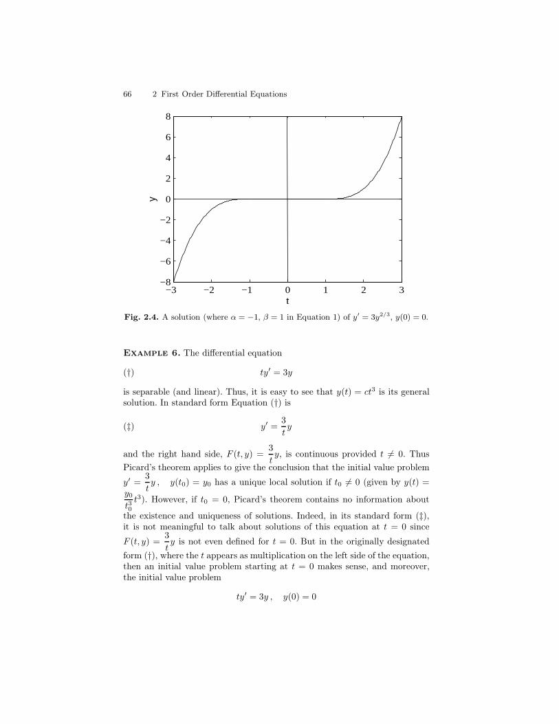
66 2 First Order Differential Equations
−3 −2 −1 0 1 2 3−8
−6
−4
−2
0
2
4
6
8
t
y
Fig. 2.4. A solution (where α = −1, β = 1 in Equation 1) of y′ = 3y2/3, y(0) = 0.
Example 6. The differential equation
(†) ty′ = 3y
is separable (and linear). Thus, it is easy to see that y(t) = ct3 is its generalsolution. In standard form Equation (†) is
(‡) y′ =3
ty
and the right hand side, F (t, y) =3
ty, is continuous provided t 6= 0. Thus
Picard’s theorem applies to give the conclusion that the initial value problem
y′ =3
ty , y(t0) = y0 has a unique local solution if t0 6= 0 (given by y(t) =
y0t30t3). However, if t0 = 0, Picard’s theorem contains no information about
the existence and uniqueness of solutions. Indeed, in its standard form (‡),it is not meaningful to talk about solutions of this equation at t = 0 since
F (t, y) =3
ty is not even defined for t = 0. But in the originally designated
form (†), where the t appears as multiplication on the left side of the equation,then an initial value problem starting at t = 0 makes sense, and moreover,the initial value problem
ty′ = 3y , y(0) = 0
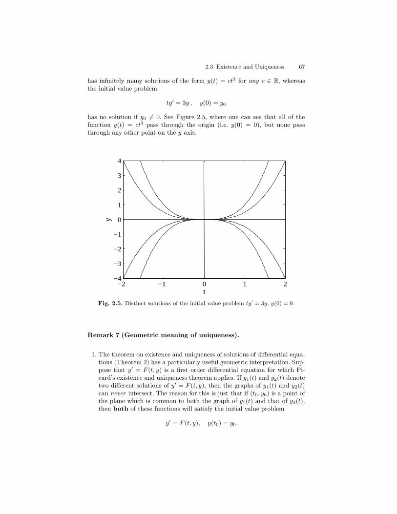
2.3 Existence and Uniqueness 67
has infinitely many solutions of the form y(t) = ct3 for any c ∈ R, whereasthe initial value problem
ty′ = 3y , y(0) = y0
has no solution if y0 6= 0. See Figure 2.5, where one can see that all of thefunction y(t) = ct3 pass through the origin (i.e. y(0) = 0), but none passthrough any other point on the y-axis.
−2 −1 0 1 2−4
−3
−2
−1
0
1
2
3
4
t
y
Fig. 2.5. Distinct solutions of the initial value problem ty′ = 3y, y(0) = 0.
Remark 7 (Geometric meaning of uniqueness).
1. The theorem on existence and uniqueness of solutions of differential equa-tions (Theorem 2) has a particularly useful geometric interpretation. Sup-pose that y′ = F (t, y) is a first order differential equation for which Pi-card’s existence and uniqueness theorem applies. If y1(t) and y2(t) denotetwo different solutions of y′ = F (t, y), then the graphs of y1(t) and y2(t)can never intersect. The reason for this is just that if (t0, y0) is a point ofthe plane which is common to both the graph of y1(t) and that of y2(t),then both of these functions will satisfy the initial value problem
y′ = F (t, y), y(t0) = y0.
68 2 First Order Differential Equations
But if y1(t) and y2(t) are different functions, this will violate the unique-ness provision of Picard’s theorem. Thus the situation depicted in Figures2.4 and 2.5 where several solutions of the same differential equation gothrough the same point (in this case (0, 0)) can never occur for a differen-tial equation which satisfies the hypotheses of Theorem 2. Similarly, thegraphs of the function y1(t) = (t+1)2 and the constant function y2(t) = 1both pass through the point (0, 1), and thus both cannot be solutions ofthe same differential equation satisfying Picard’s theorem.
2. The above remark can be exploited in the following way. The constantfunction y1(t) = 0 is a solution to the differential equation y′ = y3 + y(check it). Since F (t, y) = y3+y clearly has continuous partial derivatives,Picard’s theorem applies. Hence, if y2(t) is a solution of the equation forwhich y2(0) = 1, the above observation takes the form of stating thaty2(t) > 0 for all t. This is because, in order for y(t) to ever be negative,it must first cross the t-axis, which is the graph of y1(t), and we haveobserved that two solutions of the same differential equation can nevercross. This observation will be further exploited in the next section.
Exercises
1. a) Find the exact solution of the initial value problem
(∗) y′ = y2, y(0) = 1.
b) Apply Picard’s method (Theorem 2) to calculate the first three approxima-tions y1(t), y2(t), and y3(t) to (∗) and compare these results with the exactsolution.
I Solution. (a) The equation is separable so separate the variables to gety−2dy = dt. Integrating gives −y−1 = t + c and the initial condition y(0) = 1implies that the integration constant c = −1, so that the exact solution of (∗)is
y(t) =1
1 − t= 1 + t + t2 + t3 + t4 + · · · ; |t| < 1.
(b) To apply Picard’s method, let y0 = 1 and define
y1(t) = 1 + t
0
(y0(s))2 ds = 1 + t
0
ds = 1 + t;
y2(t) = 1 + t
0
(y1(s))2 ds = 1 + t
0
(1 + s)2 ds = 1 + t + t2 +t3
3;
y3(t) = 1 + t
0
(y2(s))2 ds = t
0 1 + s + s2 +s3
3 2
ds
= 1 + t
0 1 + 2s + 3s2 +8
3s3 +
5
3s4 +
2
3s5 +
1
9s6 ds
= 1 + t + t2 + t3 +2
3t4 +
1
3t5 +
1
9t6 +
1
63t7.
2.3 Existence and Uniqueness 69
Comparing y3(t) to the exact solution, we see that the series agree up to order3. J
2. Apply Picard’s method to calculate the first three approximations y1(t), y2(t),y3(t) to the solution y(t) of the initial value problem
y′ = t − y, y(0) = 1.
3. Apply Picard’s method to calculate the first three approximations y1(t), y2(t),y3(t) to the solution y(t) of the initial value problem
y′ = t + y2, y(0) = 0.
Which of the following initial value problems are guaranteed a unique solutionby Picard’s theorem (Theorem 2)? Explain.
4. y′ = 1 + y2, y(0) = 0
5. y′ =√
y, y(1) = 0
6. y′ =√
y, y(0) = 1
7. y′ =t − y
t + y, y(0) = −1
8. y′ =t − y
t + y, y(1) = −1
9. a) Find the general solution of the differential equation
(†) ty′ = 2y − t.
Sketch several specific solutions from this general solution.b) Show that there is no solution to (†) satisfying the initial condition y(0) = 2.
Why does this not contradict Theorem 2?
10. a) Let t0, y0 be arbitrary and consider the initial value problem
y′ = y2, y(t0) = y0.
Explain why Theorem 2 guarantees that this initial value problem has asolution on some interval |t − t0| ≤ h.
b) Since F (t, y) = y2 and Fy(t, y) = 2y are continuous on all of the (t, y)−plane,one might hope that the solutions are defined for all real numbers t. Showthat this is not the case by finding a solution of y′ = y2 which is definedfor all t ∈ R and another solution which is not defined for all t ∈ R. (Hint:Find the solutions with (t0, y0) = (0, 0) and (0, 1).)
11. Is it possible to find a function F (t, y) that is continuous and has a continuouspartial derivative Fy(t, y) such that the two functions y1(t) = t and y2(t) =t2 − 2t are both solutions to y′ = F (t, y) on an interval containing 0?
12. Show that the function
y1(t) = 0, for t < 0
t3 for t ≥ 0
is a solution of the initial value problem ty′ = 3y, y(0) = 0. Show that y2(t) = 0for all t is a second solution. Explain why this does not contradict Theorem 2.
70 2 First Order Differential Equations
2.4 Miscellaneous Nonlinear First Order Equations
We have learned how to find explicit solutions for the standard first orderdifferential equation
y′ = F (t, y)
when the right hand side of the equation has one of the particularly simpleforms:
1. F (t, y) = h(t)g(y), i.e., the equation is separable, or2. F (t, y) = −p(t)y + f(t), i.e., the equation is linear.
Unfortunately, in contrast to the separable and first order linear differentialequations, for an arbitrary function F (t, y) it is very difficult to find closedform “solution formulas”. In fact, most differential equations do not have closedform solutions and one has to resort to numerical or asymptotic approximationmethods to gain information about them. In this section we discuss some othertypes of first-order equations which you may run across in applications andthat allow closed form solutions in the same sense as the separable and first or-der linear differential equations. That is, the ”explicit" solution may very wellinvolve the computation of an indefinite integral which cannot be expressedin terms of elementary functions, or the solution may be given implicitly byan equation which cannot be reasonably solved in terms of elementary func-tion. Our main purpose in this section is to demonstrate techniques that allowus to find solutions of these types of first-order differential equations and wecompletely disregard in this section questions of continuity, differentiability,vanishing divisors, and so on. If you are interested in the huge literature cov-ering other special types of first order differential equations for which closedform solutions can be found, we refer you to books like [Zw] or to one ofthe three M’s (Mathematica, Maple, or MatLab) which are, most likely, moreefficient in computing closed form solutions than most of us will ever be.
Exact Differential Equations
A particularly important class of nonlinear first order differential equationsthat can be solved (explicitly or implicitly) is that of exact first order equa-tions. To explain the mathematics behind exact equations, it is necessary torecall some facts about calculus of functions of two variables.3 Let V (t, y) bea function of two variables defined on a rectangle
R := (t, y) : a ≤ t ≤ b , c ≤ y ≤ d .
The curve with equation V (t, y) = c, where c ∈ R is a constant, is a levelcurve of V .
3The facts needed will be found in any calculus textbook. For example, you mayconsult Chapter 14 of Calculus: Early Transcendentals, Fourth Edition by JamesStewart, Brooks-Cole, 1999.
2.4 Miscellaneous Nonlinear First Order Equations 71
Example 1. 1. If V (t, y) = t + 2y, the level curves are all of the linest+ 2y = c of slope −0.5.
2. If V (t, y) = t2 + y2, the level curves are the circles t2 + y2 = c centeredat (0, 0) of radius
√c, provided c > 0. If c = 0, then the level “curve"
t2 + y2 = 0 consists of the single point (0, 0), while if c < 0 there are nopoints at all which solve the equation t2 + y2 = c.
3. If V (t, y) = t2−y2 then the level curves of V are the hyperbolas t2−y2 = cif c 6= 0, while the level curve t2− y2 = 0 consists of the two lines y = ±t.
4. If V (t, y) = y2 − t then the level curves are the parabolas y2 − t = c withaxis of symmetry the t-axis and opening to the right.
Thus we see that sometimes a level curve defines y explicitly as a functionof t (for example, y = 1
2 (c − t) in number 1 above), sometimes t is definedexplicitly as a function of y (for example, t = −2y + c in number 1, andt = y2− c in number 3 above), while in other cases it may only be possible todefine y as a function of t (or t as a function of y) implicitly by the level curveequation V (t, y) = c. For instance, the level curve t2 +y2 = c for c > 0 definesy as a function of t in two ways (y = ±
√c− t2 for −√c < t <
√c) and it also
defines t as a function of y in two ways (t = ±√
c− y2 for −√c < y <√c).
If we are given a two variable function V (t, y) is there anything which canbe said about all of the level curves V (t, y) = c? The answer is yes. What thelevel curves of a fixed two variable function have in common is that every oneof the functions y(t) defined implicitly by V (t, y) = c, no matter what c is, isa solution of the same differential equation. The mathematics underlying thisobservation is the chain rule in two variables, which implies that
d
dtV (t, y(t)) = Vt(t, y(t)) + Vy(t, y(t))y′(t),
where Vt, Vy denote the partial derivatives of V (t, y) with respect to t and y,respectively. Thus, if a function y(t) is given implicitly by a level curve
V (t, y(t)) = c,
then y(t) satisfies the equation
0 =d
dtc =
d
dtV (t, y(t)) = Vt(t, y(t)) + Vy(t, y(t))y′(t).
This means that y(t) is a solution of the differential equation
Vt(t, y) + Vy(t, y)y′ = 0. (1)
Notice that the constant c does not appear anywhere in this equation so thatevery function y(t) determined implicitly by a level curve of V (t, y) satisfiesthis same equation. An equation of the form given by Equation 1 is referredto as an exact equation:
72 2 First Order Differential Equations
Definition 2. A differential equation written in the form
M(t, y) +N(t, y)y′ = 0
is said to be exact if there is a function V (t, y) such that M(t, y) = Vt(t, y)and N(t, y) = Vy(t, y).
What we observed above is that, if y(t) is defined implicitly by a level curveV (t, y) = c, then y(t) is a solution of the exact equation 1. Moreover, the levelcurves determine all of the solutions of Equation 1, so the general solution isdefined by
V (t, y) = c. (2)
Example 3. 1. The exact differential equation determined by V (t, y) =t+ 2y is
0 = Vt(t, y) + Vy(t, y)y′ = 1 + 2y′
so the general solution of 1 + 2y′ = 0 is t+ 2y = c.2. The exact differential equation determined by V (t, y) = t2 + y2 is
0 = Vt(t, y) + Vy(t, y)y′ = 2t+ 2yy′.
Hence, the general solution of the equation t + yy′ = 0, which can bewritten in standard form as y′ = −t/y , is t2 + y2 = c.
Suppose we are given a differential equation in the form
M(t, y) +N(t, y)y′ = 0,
but we are not given apriori thatM(t, y) = Vt(t, y) andN(t, y) = Vy(t, y). Howcan we determine if there is such a function V (t, y), and if there is, how canwe find it? That is, is there a criterion for determining if a given differentialequation is exact, and if so is there a procedure for producing the functionV (t, y) whose level curves implicitly determine the solutions. The answer toboth questions is yes. The criterion for exactness is given by the followingtheorem; the procedure for finding V (t, y) will be illustrated by example.
Theorem 4 (Criterion for exactness).A first order differential equation
M(t, y) +N(t, y)y′ = 0
in which M(t, y) and N(t, y) have continuous first order partial derivatives isexact if and only if
My(t, y) = Nt(t, y) (3)
for all t, y in a square region of R2.
2.4 Miscellaneous Nonlinear First Order Equations 73
Proof. Recall (from your calculus course) that all functions V (t, y) whosesecond partial derivatives exist and are continuous satisfy
(∗) Vty(t, y) = Vyt(t, y),
where Vty(t, y) denotes the derivative of Vt(t, y) with respect to y, and Vyt(t, y)is the derivative of Vy(t, y) with respect to t. The equation (∗) is known asClairaut’s theorem (after Alexis Clairaut (1713 – 1765)) on the equality ofmixed partial derivatives. If the equation M(t, y)+N(t, y)y′ = 0 is exact then(by definition) there is a function V (t, y) such that Vt(t, y) = M(t, y) andVy(t, y) = N(t, y). Then by Clairaut’s theorem,
My(t, y) =∂
∂yVt(t, y) = Vty(t, y) = Vyt(t, y) =
∂
∂tVy(t, y) = Nt(t, y).
Hence condition 3 is satisfied.Now assume, conversely, that condition 3 is satisfied. To verify that the
equation M(t, y) + N(t, y)y′ = 0 is exact, we need to search for a functionV (t, y) which satisfies the equations
Vt(t, y) = M(t, y) and Vy(t, y) = N(t, y).
The procedure will be sketched and then illustrated by means of an example.The equation Vt(t, y) = M(t, y) means that we should be able to recoverV (t, y) from M(t, y) by indefinite integration:
V (t, y) =
∫
M(t, y) dt+ ϕ(y). (4)
The function ϕ(y) appears as the “integration constant" since any function ofy goes to 0 when differentiated with respect to t. The function ϕ(y) can bedetermined from the equation
Vy(t, y) =∂
∂y
∫
M(t, y) dt+ ϕ′(y) = N(t, y). (5)
That is
ϕ′(y) = N(t, y)− ∂
∂y
∫
M(t, y) dt. (6)
The verification that the function on the right is really a function only of y(as it must be if it is to be ϕ′(y)) is where condition 3 is needed. ut
Example 5. Solve the differential equation y′ =t− yt+ y
I Solution. We rewrite the equation in the form y − t + (t + y)y′ = 0 toget that M(t, y) = y − t and N(t, y) = y + t. Since My(t, y) = 1 = Nt(t, y), itfollows that the equation is exact and the general solution will have the form
74 2 First Order Differential Equations
V (t, y) = c, where Vt(t, y) = y − t and Vy(t, y) = y + t. Since Vt(t, y) = y − tit follows that
V (t, y) =
∫
(y − t) dt+ ϕ(y) = yt− t2
2+ ϕ(y),
where ϕ(y) is a yet to be determined function depending on y, but not on t.To determine ϕ(y) note that y + t = Vy(t, y) = t + ϕ′(y), so that ϕ′(y) = y.Hence
ϕ(y) =y2
2+ c1
for some arbitrary constant c1, and thus
V (t, y) = yt− t2
2+y2
2+ c1.
The general solution of y′ =t− yt+ y
is therefore given by the implicit equation
V (t, y) = yt− t2
2+y2
2+ c1 = c.
This is the form of the solution which we are led to by our general solutionprocedure outlined in the proof of Theorem 4. However, after further simpli-fying this equation and renaming constants several times the general solutioncan be expressed implicitly by
2yt− t2 + y2 = c,
and explicitly byy(t) = −t±
√
2t2 + c.
J
What happens if we try to solve by equation M(t, y) + N(t, y)y′ = 0 bythe procedure outlined above without first verifying that it is exact? If theequation is not exact, you will discover this fact when you get to Equation 6,since ϕ′(y) will not be a function only of y, as the following example illustrates.
Example 6. Try to solve the equation (t − 3y) + (2t + y)y′ = 0 by thesolution procedure for exact equations.
I Solution. Note that M(t, y) = t − 3y and N(t, y) = 2t + y. First applyEquation 4 to get
(†) V (t, y) =
∫
M(t, y), dt =
∫
(t− 3y) dt =t2
2− 3ty + ϕ(y),
and then determine ϕ(y) from Equation 6:
2.4 Miscellaneous Nonlinear First Order Equations 75
(‡)ϕ′(y) = N(t, y)− ∂
∂y
∫
M(t, y) dt = (2t+ y)− ∂
∂y
(
t2
2− 3ty + ϕ(y)
)
= y− t.
But we see that there is a problem since ϕ′(y) in (‡) involves both y andt. This is where it becomes obvious that you are not dealing with an exactequation, and you cannot proceed with this procedure. Indeed, My(t, y) =−3 6= 2 = Nt(t, y), so that this equation fails the exactness criterion 3. J
Bernoulli Equations
It is sometimes possible to change the variables in a differential equationy′ = F (t, y) so that in the new variables the equation appears in a form youalready know how to solve. This is reminiscent of the substitution procedurefor computing integrals. We will illustrate the procedure with a class of equa-tions known as Bernoulli equations (named after Jakoub Bernoulli, (1654– 1705)), which are equations of the form
y′ + p(t)y = f(t)yn. (7)
If n = 0 this equation is linear, while if n = 1 the equation is both separableand linear. Thus, it is the cases n 6= 0, 1 where a new technique is needed.Start by dividing Equation 7 by yn to get
(∗) y−ny′ + p(t)y1−n = f(t),
and notice that if we introduce a new variable z = y1−n, then the chain rulegives
z′ =dz
dt=dz
dy
dy
dt= (1− n)y−ny′,
and Equation (∗), after multiplying by the constant (1−n), becomes a linearfirst order differential equation in the variables t, z:
(∗∗) z′ + (1 − n)p(t)z = f(t).
Equation (∗∗) can then be solved by Algorithm 5, and the solution to 7 isobtained by solving z = y1−n for y.
Example 7. Solve the Bernoulli equation y′ + y = y2.
I Solution. In this equation n = 2, so if we let z = y1−2 = y−1, we getz′ = −y−2y′. After dividing our equation by y2 we get y−2y′+y−1 = 1, whichin terms of the variable z is −z′ + z = 1. In the standard form for linearequations this becomes
z′ − z = −1.
We can apply Algorithm 5 to this equation. The integrating factor will be e−t.Multiplying by the integrating factor gives (e−1z)′ = −e−t so that e−tz =
76 2 First Order Differential Equations
e−t + c. Hence z = 1 + cet. Now go back to the original function y by solvingz = y−1 for y. Thus
y = z−1 = (1 + cet)−1 =1
1 + cet
is the general solution of the Bernoulli equation y′ + y = y2.Note that this equation is also a separable equation, so it could have been
solved by the technique for separable equations, but the integration (andsubsequent algebra) involved in the current procedure is simpler. J
There are a number of other types of substitutions which are used totransform certain differential equations into a form which is more amenablefor solution. We will not pursue the topic further in this text. See the book[Zw] for a collection of many different solution algorithms.
Exercises
Exact EquationsFor Exercises 1 – 9, determine if the equation is exact, and if it is exact, find the
general solution.
1. (y2 + 2t) + 2tyy′ = 0
I Solution. This can be written in the form M(t, y) + N(t, y)y′ = 0 whereM(t, y) = y2+2t and N(t, y) = 2ty. Since My(t, y) = 2y = Nt(t, y), the equationis exact (see Equation (3.2.2)), and the general solution is given implicitly byF (t, y) = c where the function F (t, y) is determined by Ft(t, y) = M(t, y) = y2+2t and Fy(t, y) = N(t, y) = 2ty. These equations imply that F (t, y) = t2 + ty2
will work so the solutions are given implicitly by t2 + ty2 = c. J
2. y − t + ty′ + 2yy′ = 0
3. 2t2 − y + (t + y2)y′ = 0
4. y2 + 2tyy′ + 3t2 = 0
5. (3y − 5t) + 2yy′ − ty′ = 0
6. 2ty + (t2 + 3y2)y′ = 0, y(1) = 1
7. 2ty + 2t2 + (t2 − y)y′ = 0
8. t2 − y − ty′ = 0
9. (y3 − t)y′ = y
10. Find conditions on the constants a, b, c, d which guarantee that the differentialequation (at + by) = (ct + dy)y′ is exact.Bernoulli Equations. Find the general solution of each of the followingBernoulli equations. If an initial value is given, also solve the initial value prob-lem.
2.4 Miscellaneous Nonlinear First Order Equations 77
11. y′ − y = ty2, y(0) = 1
12. y′ + ty = t3y3
13. (1 − t2)y′ − ty = 5ty2
14. y′ + ty = ty3
15. y′ + y = ty3
General Equations. The following problems may any of the types studied sofar.
16. y′ = ty − t, y(1) = 2
17. (t2 + 3y2)y′ = −2ty
18. t(t + 1)y′ = 2√
y
19. y′ =y
t2 + 2t − 3
20. sin y + y cos t + 2t + (t cos y + sin t)y′ = 0
21. y′ +1
t(t − 1)y = t − 1
22. y′ − y = 12ety−1, y(0) = −1
23. y′ =8t2 − 2y
t
24. y′ =y2
t, y(1) = 1

3
The Laplace Transform
In this chapter we introduce the Laplace Transform and show how it givesa direct method for solving certain initial value problems. This technique isextremely important in applications since it gives an easily codified procedurethat goes directly to the solution of an initial value problem without firstdetermining the general solution of the differential equation. The same theo-retical procedure applies to ordinary differential equations of arbitrary order(with constant coefficients) and even to systems of constant coefficient linearordinary differential equations, which will be treated in Chapter 10. Moreoverthe same procedure applies to linear constant coefficient equations (of anyorder) for which the forcing function is not necessarily continuous. This willbe addressed in Chapter 8.
You are already familiar with certain operators which transform one func-tion into another. One particularly important example is the differentiationoperator D which transforms each function which has a derivative into itsderivative, i.e., D(f) = f ′. The Laplace transform L is an integral operatoron certain spaces of functions on the interval [0, ∞). By an integral opera-tor, we mean an operator T which takes an input function f and transformsit into another function F = T f by means of integration with a kernelfunction K(s, t). That is,
T f(t) =
∫ ∞
0
K(s, t)f(t) dt = F (s).
The Laplace transform is the particular integral transform obtained by usingthe kernel function
K(s, t) = e−st.
When applied to a (constant coefficient linear) differential equation theLaplace transform turns it into an algebraic equation, one that is generallymuch easier to solve. After solving the algebraic equation one needs to trans-form the solution of the algebraic equation back into a function that is the
80 3 The Laplace Transform
solution to the original differential equation. This last step is known as theinversion problem.
This process of transformation and inversion is analogous to the use of thelogarithm to solve a multiplication problem. When scientific and engineeringcalculations were done by hand, the standard procedure for doing multiplica-tion was to use logarithm tables to turn the multiplication problem into anaddition problem. Addition, by hand, is much easier than multiplication. Af-ter performing the addition, the log tables were used again, in reverse order,to complete the calculation. Now that calculators are universally available,multiplication is no more difficult than addition (one button is as easy topush as another) and the use of log tables as a tool for multiplication is es-sentially extinct. The same cannot be said for the use of Laplace transformsas a tool for solving ordinary differential equations. The use of sophisticatedmathematical software (Maple, Mathematica, MatLab) can simplify many ofthe routine calculations necessary to apply the Laplace transform, but it in noway absolves us of the necessity of having a firm theoretical understanding ofthe underlying mathematics, so that we can legitimately interpret the num-bers and pictures provided by the computer. For the purposes of this course,we provide a table (Table C.2) of Laplace transforms for many of the commonfunctions you are likely to see. This will provide a basis for studying manyexamples.
3.1 Definition and Basic Formulas for the Laplace
Transform
Suppose f(t) is a continuous function defined for all t ≥ 0. The Laplacetransform of f is the function Lf(t) (s) = F (s) defined by the equation
F (s) = Lf(t) (s) =
∫ ∞
0
e−stf(t) dt = limr→∞
∫ r
0
e−stf(t) dt (1)
provided the limit exists for all sufficiently large s. This means that there isa number N , which will depend on the function f , so that the limit existswhenever s > N . If there is no such N , then the function f will not have aLaplace transform. It can be shown that if the Laplace transform exists ats = N then it exists for all s ≥ N .
Let’s analyze this equation somewhat further. The function f with whichwe start will sometimes be called the input function. Generally, ‘t’ willdenote the variable for an input function f , while the Laplace transform of f ,denoted Lf(t) (s),1 is a new function (the output function or transform
1Technically, f is the function while f(t) is the value of the function f at t. Thus,to be correct the notation should be Lf (s). However, there are times when thevariable t needs to be emphasized or f is given by a formula such as in L e2t (s).Thus we will freely use both notations: Lf(t) (s) and Lf (s).
3.1 Definition and Basic Formulas for the Laplace Transform 81
function), whose variable will usually be ‘s’. Thus Equation (1) is a formulafor computing the value of the function Lf at the particular point s, sothat, in particular
F (2) = Lf (2) =
∫ ∞
0
e−2tf(t) dt
and F (−3) = Lf (−3) =
∫ ∞
0
e3tf(t) dt,
provided s = 2 and s = −3 are in the domain of Lf(t).When possible, we will use a lower case letter to denote the input function
and the corresponding uppercase letter to denote its Laplace transform. Thus,F (s) is the Laplace transform of f(t), Y (s) is the Laplace transform of y(t),etc. Hence there are two distinct notations that we will be using for the Laplacetransform of f(t); if there is no confusion we use F (s), otherwise we will writeLf(t) (s).
To avoid the notation becoming too heavy-handed, we will frequently writeLf(t) rather than Lf(t) (s). That is, the variable s may be suppressedwhen the meaning is clear. It is also worth emphasizing that, while the in-put function f has a well determined domain [0, ∞), the Laplace transformLf (s) = F (s) is only defined for all sufficiently large s, and the domain willdepend on the particular input function f . In practice, this will not be an issueand we will generally not emphasize the particular domain of F (s). We willrestrict our attention to continuous input functions in this chapter. In Chapter8, we ease this restriction and consider Laplace transforms of discontinuousfunctions.
A particularly useful property of the Laplace transform, both theoreticallyand computationally, is that of linearity. For the Laplace transform linearitymeans the following, which, because of its importance, we state formally as atheorem.
Theorem 1. The Laplace transform is linear. In other words, if f and g areinput functions and a and b are constants then
Linearity of the Laplace transform
Laf + bg = aLf+ bLg .
Proof. This follows from the fact that (improper) integration is linear. ut
Basic Laplace Transforms
Example 2. Verify the Laplace transform formula:
82 3 The Laplace Transform
Constant Functions
L1 (s) =1
s, s > 0.
I Solution. For the constant function 1 we have
L1 (s) =
∫ ∞
0
e−st · 1 dt = limr→∞
e−ts
−s
∣
∣
∣
∣
r
0
= limr→∞
e−rs − 1
−s =1
sfor s > 0.
J
Some comments are in order. The condition s > 0 is needed for the limit
limr→∞
e−rs − 1
−sthat defines the improper integral
∫∞0e−st dt to exist. This is because
limr→∞
erc =
0 if c < 0
∞ if c > 0.
More generally, it follows from L’Hôspital’s rule that
limt→∞
tnect = 0 if n ≥ 0 and c < 0. (2)
This important fact (which you learned in calculus) is used in a numberof calculations in the following manner. We will use the notation h(t)|∞aas a shorthand for limr→∞ h(t)|ra = limr→∞(h(r) − h(a)). In particular, iflimt→∞ h(t) = 0 then h(t)|∞a = −h(a), so that Equation (2) implies
tnect∣
∣
∞0
=
0 if n > 0 and c < 0
−1 if n = 0 and c < 0.(3)
Example 3. Assume n is a nonnegative integer. Verify the Laplace trans-form formula:
Power Functions
Ltn (s) =n!
sn+1, s > 0.
3.1 Definition and Basic Formulas for the Laplace Transform 83
I Solution. If n = 0 then f(t) = t0 = 1 and this case was given above.Assume now that n > 0. Then
Ltn (s) =
∫ ∞
0
e−sttn dt
and this integral can be computed using integration by parts with the choiceof u and dv given as follows:
u = tn dv = e−st dt
du = ntn−1 dt v =−e−st
s.
Using the observations concerning L’Hôspital’s rule in the previous paragraph,we find that if n > 0 and s > 0, then
Ltn (s) =
∫ ∞
0
e−sttn dt
= −tn e−st
s
∣
∣
∣
∣
∞
0
+n
s
∫ ∞
0
e−sttn−1 dt
=n
sL
tn−1
(s).
By iteration of this process (or by induction), we obtain (again assuming n > 0and s > 0)
Ltn (s) =n
sL
tn−1
(s)
=n
s· (n− 1)
sL
tn−2
(s)
...
=n
s· n− 1
s· · · 2
s· 1sL
t0
(s).
But L
t0
(s) = L1 (s) = 1/s, by Example 2. The result now follows. J
Example 4. Assume a ∈ R. Verify the Laplace transform formula:
Exponential Functions
Leat (s) =1
s− a , s > a.
84 3 The Laplace Transform
I Solution.
L
eat
(s) =
∫ ∞
0
e−steat dt =
∫ ∞
0
e−(s−a)t dt =e−(s−a)t
−(s− a)
∣
∣
∣
∣
∞
0
=1
s− a .
The last equality follows from Equation (3) provided s > a. J
We note that in this example the calculation can be justified for λ =a + ib ∈ C instead of a ∈ R, once we have noted what we mean by thecomplex exponential function. The main thing to note is that the complexexponential function ez (z ∈ C) satisfies the same rules of algebra as thereal exponential function, namely, ez1+z2 = ez1ez2 . This is achieved by simplynoting that the same power series which defines the real exponential makessense for complex values also. Recall that the exponential function ex has apower series expansion
ex =
∞∑
n=0
xn
n!
which converges for all x ∈ R. This familiar infinite series makes perfectlygood sense if x is replaced by any complex number z, and moreover, it can beshown that the resulting series converges for all z ∈ C. Thus, we define thecomplex exponential function by means of the convergent series
ez :=
∞∑
n=0
zn
n!. (4)
It can be shown that this function ez satisfies the functional equation
ez1+z2 = ez1ez2 .
Since e0 = 1, it follows that 1/ez = e−z. Taking z = it in Equation (4) leadsto an important formula for the real and imaginary parts of eit:
eit =
∞∑
n=0
(it)n
n!= 1 + it− t2
2!− i t
3
3!+t4
4!+ i
t5
5!− · · ·
= (1− t2
2!+t4
4!− · · · ) + i(t− t3
3!+t5
5!− · · · ) = cos t+ i sin t,
where one has to know (from studying calculus) that the two series in the lastline above are the Taylor series expansions for cos t and sin t, respectively. Inwords, this says that the real part of eit is cos t and the imaginary part of eit
is sin t. Combining this with the basic exponential functional property givesthe formula, known as Euler’s formula, for the real and imaginary parts ofeλt (λ = a+ bi):
eλt = e(a+bi)t = eat+ibt = eateibt = eat(cos bt+ i sin bt).
We formally state this as a theorem.
3.1 Definition and Basic Formulas for the Laplace Transform 85
Theorem 5 (Euler’s Formula). If λ = a+ bi ∈ C and t ∈ R, then
eλt = eat(cos bt+ i sin bt).
An important consequence of Euler’s formula is the limit formula
limt→∞
e(a+bi)t = 0, if a < 0.
More generally, the analog of Equation (3) is
tne(a+bi)t∣
∣
∣
∞
0=
0 if n > 0 and a < 0
−1 if n = 0 and a < 0.(5)
Example 6. Assume λ ∈ C. Verify the Laplace transform formula:
Compex Exponential Functions
L
eλt
(s) =1
s− λ, s > Reλ.
I Solution.
L
eλt
(s) =
∫ ∞
0
e−steλt dt
=
∫ ∞
0
e−(s−λ)t dt =e−(s−λ)t
−(s− λ)
∣
∣
∣
∣
∞
0
=1
s− λ.
The last equality follows from Equation (5), provided the real part of the coef-ficient of t in the exponential, i.e., −(s−Reλ), is negative. That is, provideds > Reλ. J
Complex-Valued Functions
When we are given a problem that can be stated in the domain of the realnumbers it can sometimes be advantageous to recast that same problem inthe domain of the complex numbers. In many circumstances the resolution ofthe problem is easier over the complex numbers. This important concept willrecur several times throughout this text.
Let λ = a + ib. Euler’s formula, eλt = e(a+ib)t = eat(cos bt + i sin bt),introduces the concept of a complex-valued function. Let us say a few generalwords about this notion.
A complex valued function z defined on an interval I in R is a functionof the form
86 3 The Laplace Transform
z(t) = x(t) + iy(t), t ∈ I.Here, x(t) and y(t) are real valued functions, x(t) is called the real part ofz(t), and y(t) is called the imaginary part of z(t). Thus eibt is a complexvalued function with real part cos bt and imaginary part sin bt. The notionsof limits, continuity, differentiability, and integrability, all extend to complexvalued functions. In fact, since the complex numbers can be identified with theEuclidean plane, R2, with i = (0, 1), we can also identify complex-valued func-tions with vector-valued (R2-valued) functions written in the form (x(t), y(t)).In the context of R2-valued functions, differentiation and integration are per-formed component-wise. Thus z(t) is differentiable if and only if the realand imaginary parts of z are differentiable and
z′(t) = x′(t) + iy′(t).
Thus, if z(t) = cos t+i sin t = eit then z′(t) = − sin t+i cos t = ieit. In fact, forany complex number γ it is easy to verify that the derivative of eγt is γeγt. Thesecond derivative is given by z′′(t) = x′′(t)+iy′′(t) and higher order derivativesare analogous. The usual product and quotient rules for differentiation applyfor complex valued functions. Similarly, z(t) is integrable on an interval [a, b]if and only if the real and imaginary parts are integrable on [a, b]. We thenhave
∫ b
a
z(t) dt =
∫ b
a
x(t) dt+ i
∫ b
a
y(t) dt.
We define the Laplace transform of z(t) by the integral formula
Lz(t)(s) =
∫ ∞
0
e−stz(t) dt,
provided the integral is finite for all s > N for some N . In this case we say z(t)has a Laplace transform. It is easy to see that z(t) has a Laplace transform ifand only if the real and imaginary parts of z have Laplace transforms and
Lz(t) (s) = Lx(t) (s) + iLy(t) (s).
The notion of linearity introduced in Theorem 1 applies to complex-valuedfunctions and complex scalars. Since e−st is real-valued we have Re e−stz(t) =e−stx(t) and Im e−stz(t) = e−sty(t) and this simple observation implies
Theorem 7. Suppose z(t) = x(t) + iy(t), where x(t) and y(t) are real-valuedfunctions have Laplace transforms. Then
ReLz(t) (s) = Lx(t) (s)
ImLz(t) (s) = Ly(t) (s).
Example 8. Let z(t) = e2t + it2. Find z′(t),∫ 1
0 z(t) dt, and Lz(t) (s).
3.1 Definition and Basic Formulas for the Laplace Transform 87
I Solution.
z′(t) = 2e2t + 2it
∫ 1
0
z(t) dt =e2t
2+ i
t3
3
∣
∣
∣
∣
1
0
=e2 − 1
2+ i
1
3
Lz(t) (s) =1
s− 2+ i
2
s3=s3 + i2(s− 2)
s3(s− 2).
J
With these simple concepts and observations about complex-valued func-tions in mind we now return to establishing basic Laplace transform formulas.
Example 9. Let b ∈ R. Verify the Laplace transform formulas:
Cosine Functions
Lcos bt (s) =s
s2 + b2, for s > 0.
and
Sine Functions
Lsin bt (s) =b
s2 + b2, for s > 0.
I Solution. A direct application of the definition of the Laplace Transformapplied to sin bt or cos bt would each require two integrations by parts; atedious calculation. As indicated above reframing the problem in the contextof complex-valued functions sometimes simplify matters substantially. This isthe case here. We use Equation (6) with λ = ib to get
L
eibt
(s) =1
s− ib=
1
s− ibs+ ib
s+ ib=
s+ ib
s2 + b2
=s
s2 + b2+ i
b
s2 + b2
On the other hand, Euler’s formula and linearity gives
88 3 The Laplace Transform
L
eibt
(s) = Lcos bt+ i sin bt (s)= Lcos bt (s) + iLsin bt (s).
By equating the real and imaginary parts, as in Theorem 7, we obtain
Lcos bt (s) =s
s2 + b2and Lsin bt (s) =
b
s2 + b2, for s > 0.
J
Example 10. Let n be a nonnegative integer and a ∈ R. Verify the followingLaplace transform formula:
Simple Exponential Polynomial
Ltneat (s) =n!
(s− a)n+1, for s > a.
I Solution. Notice that
L
tneat
(s) =
∫ ∞
0
e−sttneat dt =
∫ ∞
0
e−(s−a)tn dt = Ltn (s− a).
What this formula says is that the Laplace transform of the function tneat
evaluated at the point s is the same as the Laplace transform of the functiontn evaluated at the point s− a. Since Ltn (s) = n!/sn+1, we conclude
L
tneat
(s) =n!
(s− a)n+1, for s > a.
J
The same proof gives the following
Example 11. Let n be a nonnegative integer and λ ∈ C. Verify the followingLaplace transform formula:
Simple Complex Exponential Polynomial
L
tneλt
(s) =n!
(s− λ)n+1, for s > Reλ.
If the function tn in Example 10 is replaced by an arbitrary function f(t)with a Laplace transform F (s), then we obtain the following:
3.1 Definition and Basic Formulas for the Laplace Transform 89
Theorem 12. Suppose f has Laplace transform F (s). Then
First Translation Principle
Leatf(t) (s) = F (s− a).
Proof.
L
eatf(t)
(s) =
∫ ∞
0
e−steatf(t) dt
=
∫ ∞
0
e−(s−a)f(t) dt
= Lf(t) (s− a) = F (s− a).
utIn words, this formula says that to compute the Laplace transform of f(t)
multiplied by eat, then it is only necessary to take the Laplace transform off(t) (namely, F (s)) and replace the variable s by s−a, where a is the coefficientof t in the exponential multiplier. Here is an example of this formula in use.
Example 13. Suppose a, b ∈ R. Verify the Laplace transform formulas
L
eat cos bt
(s) =s− a
(s− a)2 + b2
and
L
eat sin bt
(s) =b
(s− a)2 + b2.
I Solution. From Example 9 we know that
Lcos bt (s) =s
s2 + b2and Lsin bt (s) =
b
s2 + b2.
Replacing s by s− a in each of these formulas gives the result. J
For a numerical example, note that
L
e−t sin 3t
=3
(s+ 1)2 + 9and L
e3t cos√
2t
=s− 3
(s− 3)2 + 2.
90 3 The Laplace Transform
Example 14. Suppose n is a nonnegative integer and λ = a+ib ∈ C. Verifythe following Laplace transform formulas:
Ltneat cos bt (s) = Re
(
n!
(s− λ)n+1
)
=n! Re
(
(s− λ)n+1)
((s− a)2 + b2)n+1
and
Ltneat sin bt (s) = Im
(
n!
(s− λ)n+1
)
=n! Im
(
(s− λ)n+1)
((s− a)2 + b2)n+1.
I Solution. Let λ = a+ bi. Then Euler’s formula gives
eλt = eat(cos bt+ i sin bt)
and hencetneλt = tneat cos bt+ itneat sin bt.
That is, tneat cos bt is the real part and tneat sin bt is the imaginary part oftneλt. By the First Translation principle (or, more directly, from Example 11)
L
tneλt
(s) =n!
(s− λ)n+1.
The formulas follow now from Theorem 7. J
Notice that when n = 0 in Example 14 the formula reduces to those givenin Example 13. We need only observe that
1
s− λ =1
(s− a)− ib
=1
(s− a)− ib ·(s− a) + ib
(s− a) + ib
=(s− a) + ib
(s− a)2 + b2
and equate real and imaginary parts.If we take n = 1 in the above example, then
1
(s− λ)2 =1
((s− a)− ib)2
=1
((s− a)− ib)2 ·((s− a) + ib)2
((s− a) + ib)2
=((s− a)2 − b2) + i2(s− a)b
((s− a)2 + b2)2.
3.1 Definition and Basic Formulas for the Laplace Transform 91
By taking real and imaginary parts of this last expression, we conclude that
L
teat cos bt
(s) =(s− a)2 − b2
((s− a)2 + b2)2
and L
teat sin bt
(s) =2(s− a)b
((s− a)2 + b2)2.
There are general formulas for n > 1 but they are difficult to remember andnot very instructive. We will not give them here.
We now summarize in Table 3.1 the basic Laplace transform formulaswe have derived. The student should learn these well as they will be usedfrequently throughout the text and exercises. As we continue several new for-mulas will be derived. Table C.2, in the appendix to this text, has a completelist of Laplace transform formulas that we have derived.
With the use of the Table and linearity we can find the Laplace transformof many functions. Consider the following examples.
Example 15. Find the Laplace transform of the following functions
1. 3− 2t3 − 3e−3t
2. 3 sin 2t+ te2t
3. e6t cos 3t
4. e(1+2i)t
5. sin2 t6. t2e−3t sin t
I Solution.
1. L3− 2t3 − 3e−3t = 3L1 − 2Lt3 − 3Le−3t
= 31
s− 2
3!
s4− 3
1
s+ 3=
9s3 − 12s− 36
s4(s+ 3)
2. L3 sin 2t+ te2t = 3Lsin 2t+ Lte2t
= 32
s2 + 22+
1
(s− 2)2=
7s2 − 24s+ 28
(s2 + 4)(s− 2)2
3. Le6t cos 3t =s− 6
(s− 6)2 + 32=
s− 6
s2 − 12s+ 45
4. Le(1+2i)t =1
s− (1 + 2i)=
1
(s− 1)− 2i· (s− 1) + 2i
(s− 1) + 2i
=(s− 1) + 2i
(s− 1)2 + 4=
(s− 1) + 2i
s2 − 2s+ 5
5. The function sin2 t does not directly appear in the table. However, the
double angle formula cos 2t = 1 − 2 sin2 t implies sin2 t =1
2(1 − cos 2t).
Thus
92 3 The Laplace Transform
Lsin2 t =1
2L1− cos 2t =
1
2
(
1
s− s
s2 + 4
)
=1
2· s
2 + 4− s2s(s2 + 4)
=2
s(s2 + 4)
6. We apply Example 14 with λ = −3 + i. First,
2
(s− λ)3 =2
((s+ 3)− i)3 ·((s+ 3) + i)3
((s+ 3) + i)3
= 2(s+ 3)3 − 3(s+ 3)2i+ 3(s+ 3)i2 − i3
((s+ 3)2 + 1)3
= 2(s+ 3)3 − 3(s+ 3) + i(−3(s+ 3)2 + 1)
((s+ 3)2 + 1)3.
Thus,
L
t2e−3t sin t
= Im2
(s− λ)3 =−6(s+ 3)2 + 2
(s2 + 6s+ 10)3.
J
We now introduce another useful principle that can be used to computesome Laplace transforms.
Theorem 16. Suppose f(t) is an input function and F (s) = Lf(t) (s) isthe transform function. Then
Transform Derivative Principle
L−tf(t) (s) =d
dsF (s).
Proof. By definition, F (s) =∫∞0e−stf(t) dt and thus
F ′(s) =d
ds
∫ ∞
0
e−stf(t) dt
=
∫ ∞
0
d
ds(e−st)f(t) dt
=
∫ ∞
0
e−st(−t)f(t) dt = L−tf(t) (s).
Passing the derivative under the integral can be justified. (c.f. ??) ut
Repeated applications of the Transform Derivative Principle gives
3.1 Definition and Basic Formulas for the Laplace Transform 93
Transform nth-Derivative Principle
(−1)nLtnf(t) (s) =dn
dsnF (s).
Example 17. Use the Transform Derivative Principle to compute
Lt sin t (s) and Lt cos t (s).
I Solution. A direct application of the Transform Derivative Principlegives
Lt sin t (s) = − d
dsLsin t (s)
= − d
ds
1
s2 + 1
= − −2s
(s2 + 1)2=
2s
(s2 + 1)2.
and Lt cos t (s) = − d
dsLcos t (s)
= − d
ds
s
s2 + 1
= − (s2 + 1)− 2ss
(s2 + 1)2=
s2 − 1
(s2 + 1)2.
J
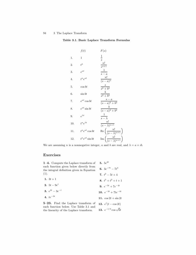
94 3 The Laplace Transform
Table 3.1. Basic Laplace Transform Formulas
f(t) F (s)
1. 11
s
2. tn n!
sn+1
3. eat 1
s − a
4. tneat n!
(s − a)n
5. cos bts
s2 + b2
6. sin btb
s2 + b2
7. eat cos bts − a
(s − a)2 + b2
8. eat sin btb
(s − a)2 + b2
9. eλt 1
s − λ
10. tneλt n!
(s − λ)n+1
11. tneat cos bt Re n!
(s − λ)n+1 12. tneat sin bt Im n!
(s − λ)n+1 We are assuming n is a nonnegative integer, a and b are real, and λ = a + ib.
Exercises
1–4. Compute the Laplace transform ofeach function given below directly fromthe integral definition given in Equation(1).
1. 3t + 1
2. 5t − 9et
3. e2t − 3e−t
4. te−3t
5–23. Find the Laplace transform ofeach function below. Use Table 3.1 andthe linearity of the Laplace transform.
5. 5e2t
6. 3e−7t − 7t3
7. t2 − 5t + 4
8. t3 + t2 + t + 1
9. e−3t + 7e−4t
10. e−3t + 7te−4t
11. cos 2t + sin 2t
12. et(t − cos 2t)
13. e−t/3 cos√
6t
3.2 Partial Fractions: A Recursive Method for Linear Terms 95
14. (t + e2t)2
15. 5 cos 2t − 3 sin 2t + 4
16. e5t(8 cos 2t + 11 sin 2t)
17. t2 sin 2t
18. e−at − e−bt for a 6= b.
19. cos2 bt (Hint: cos2 θ = 12(1 +
cos 2θ))
20. sin2 bt
21. sin bt cos bt Hint: Use an appropri-ate trigonometric identity.
22. cosh bt (Recall that cosh bt =(ebt + e−bt)/2.)
23. sinh bt (Recall that sinh bt =(ebt − e−bt)/2.)
24–30. The following problems concernbasic properties of complex valued func-tions.
24. Let λ = a+ ib and γ = c+ id. Deter-mine the real and imaginary parts ofγeλt.
25. By separating the real and imagi-nary parts verify that d
dteλt = λeλt.
26. By separating the real and imag-inary parts verity that
eλt dt =
1λeλt + C. (You will need to use in-
tegration by parts.
27. Product Rule: Suppose z(t) andw(t) are two complex valued func-tions. Verify
(z · w)′ = z′w + zw′.
28. Quotient Rule: Suppose z(t) andw(t) are two complex valued func-tions. Verify
z
w ′=
z′w − w′z
w2.
29. Chain Rule: Suppose z(t) and w(t)are two complex valued functions.Verify
(z w)′(t) = z′(w(t))w′(t).
30. Verify the limits tne(a+bi)t ∞0 =0 if n > 0 and a < 0
−1 if n = 0 and a < 0.
31. Verify that the function f(t) = et2
does not have a Laplace transform.That is, show that the improper inte-gral that defines F (s) does not con-verge for any value of s.
3.2 Partial Fractions:
A Recursive Method for Linear Terms
A careful look at Table 3.1 reveals that the Laplace transform of each functionwe considered is a rational function. The inversion of the Laplace transform,which we will discuss in detail in Sections 3.4 and 3.5, will involve writingrational functions as sums of those simpler ones found in the Table.
All students of calculus should be familiar with the technique of obtain-ing the partial fraction decomposition of a rational function. Briefly, a givenrational function p(s)/q(s) is a sum of partial fractions of the form
96 3 The Laplace Transform
Aj
(s− λ)jand
Bks+ Ck
(s2 + cs+ d)k,
where Aj , Bk, and Ck are constants. The partial fractions are determined bythe linear factors, s− λ, and the irreducible quadratic factors, s2 + cs+ d, ofthe denominator q(s), where the powers j and k occur up to the multiplicityof the factors. After finding a common denominator and equating the numer-ators we obtain a system of linear equations to solve for the undeterminedcoefficients Aj , Bk, Ck. Notice that the degree of the denominator determinesthe number of coefficients that are involved in the form of the partial fractiondecomposition. Even when the degree is relatively small this process can bevery tedious and prone to simple numerical mistakes.
Our purpose in this section and the next is to provide an alternate algo-rithm for obtaining the partial fraction decomposition of a rational function.This algorithm has the advantage that it is constructive (assuming the factor-ization of the denominator), recursive (meaning that only one coefficient at atime is determined), and self checking. This recursive method for determiningpartial fractions should be well practiced by the student. It is the method wewill use throughout the text and is an essential technique in solving nonho-mogeneous differential equations discussed in Section 4.5.
We begin by reviewing a few well known facts about polynomials and ra-tional functions. This will also give us an opportunity to set down notationand introduce some important concepts. Thereafter we will discuss the algo-rithm in the linear case, i.e. when the denominator has a linear term as afactor. In Section 3.3 we specialize to the irreducible quadratic case.
Polynomials
A real polynomial p(s) is a function of the form
p(s) = ansn + an−1s
n−1 + . . .+ a1s+ a0,
where the coefficients a0, . . . , an are real. If the coefficients are in the com-plex numbers then we say p(s) is a complex polynomial. The degreeof p(s) is n if the leading coefficient, an, is nonzero. If an = 1, we sayp(s) is a monic polynomial. Since R ⊂ C, a real polynomial may be re-garded as a complex polynomial. By separating the coefficients into theirreal and imaginary parts we can always write a complex polynomial p(s) inthe from p(s) = p1(s) + ip2(s), where p1(s) and p2(s) are real polynomi-als. The complex conjugate of p(s), written p(s), is obtained by replac-ing the coefficients by their complex conjugate. It is not hard to see thatp(s) = p1(s) − ip2(s). For example, if p(s) = 1 + i + 2s + is2 then we canwrite p(s) = 1 + 2s + i(1 + s2). The real part of p(s) is 1 + 2s, the imag-inary part is 1 + s2, and p(s) = 1 + 2s − i(1 + s2). Note that the productof two real (complex) polynomials is again a real (complex) polynomial. Itcan happen that the product of two complex polynomials is real, for example,
3.2 Partial Fractions: A Recursive Method for Linear Terms 97
(s+i)(s−i) = s2+1. More generally, p(s)p(s) is a real polynomial. Sometimeswe will refer to p(s) just as a polynomial if it is not necessary to distinguishthe real or complex case.
We also observe that the sum of two real (complex) polynomials is a real(complex) polynomial. Also the product of a real scalar and a real polynomialis again a real polynomial. In short, we say that the set of polynomials isclosed under addition and scalar multiplication. A similar statement appliesin the complex case.
Linear Spaces
This important closure property just described for polynomials can be ex-pressed in a more general setting. A set of functions, F , is called a real(complex) linear space if it is closed under addition and real (complex)scalar multiplication. In other words, F is a real linear space if
f1 + f2 ∈ F closure under addition
cf ∈ F closure under real scalar multiplication,
for f1, f2, and f in F and c ∈ R. If the scalars used are complex numbersthen F is a complex linear space. If f1, . . . , fk are functions then a linearcombination of f1, . . . , fk is a sum of the form
c1f1 + · · ·+ ckfk,
where c1, . . . , ck are scalars. When F is a linear space, i.e., closed under ad-dition and scalar multiplication, and all f1, . . . , fk are in F then all linearcombinations are back in F . This very important property of linear spaces isexploited frequently throughout this text.
Let P denote all real polynomials and PC the complex polynomials. Then,using this new language our discussion in the preceding paragraphs impliesthat P is a real linear space and PC is a complex linear space.
The fundamental theorem of algebra expresses how polynomials factor inthe real and complex cases. Let’s begin with the complex case; it’s easier.
Theorem 1 (Fundamental Theorem of Algebra over C). Let q(s) ∈PC. Then there are finitely many distinct complex numbers λ1, . . . , λr andpositive integers m1, . . . ,mk such that
q(s) = C(s− λ1)m1(s− λ2)
m2 · · · (s− λr)mk .
Each λi is a root of q(s), since p(λi) = 0. The positive integer mi isthe multiplicity of λi (or (s − λi)) in q(s). The constant C is the leading
98 3 The Laplace Transform
coefficient of q(s). Simply put, a real or complex polynomial can always befactored into a product of linear terms, s− λ.
The real version of this theorem, given below, is slightly more complicatedif we require that the all factors have real coefficients. Suppose t(s) = s2 +cs + d, where c and d are real. We say t(s) is an irreducible quadratic ift(s) cannot be factored over the real numbers, i.e., we cannot write t(s) =s2 + cs + d = (s − a1)(s − a2), with a1 and a2 real numbers. It’s easy to seethat t(s) is irreducible if and only if t(s) is strictly positive. A simple exampleis t(s) = s2 +1, since t(s) ≥ 1. To determine whether a polynomial of degree 2is irreducible we can apply the quadratic formula and check to see whether thediscriminant, c2 − 4d, is negative. The preferred, though equivalent, methodis to complete the square. Thus
t(s) = s2 + cs+ d = s2 + cs+c2
4+ d− c2
4= (s+
c
2)2 +
4d− c24
.
If 4d − c2 is positive then t(s) is a sum of a square and a positive number,hence positive and hence irreducible. Thus, irreducible quadratics, t(s), canalways we written in the form
t(s) = (s− a)2 + b2,
with a, b real and b > 0 (a = − c2 and b =
√4d−c2
2 ). Written in this way thecomplex roots can be easily read
λ = a+ ib and λ = a− ib.For example, consider t(s) = s2 + 4s + 13. Completing the square gives
t(s) = s2 + 4s+ 4 + 13− 4 = (s+ 2)2 + 9 = (s + 2)2 + 32, a sum of squares.Thus t(s) is an irreducible quadratic; it does not factor over the real numbers.However, it does factor over the complex numbers. It’s complex roots areλ = −2 + 3i and λ = −2− 3i and we can write
s2 + 4s+ 13 = (s− (−2 + 3i))(s− (−2− 3i)).
You will note that an irreducible quadratic has non real roots related bycomplex conjugation:
λ, λ
, which we refer to as a conjugate root pair.More generally, if q(s) is real and λ is a non real root then so is λ, since0 = q(λ) = q(λ) = q(λ). Clearly, both roots have the same multiplicities.This observation can be used to get the following theorem (the real case) asa consequence of the complex case, Theorem 1.
Theorem 2 (Fundamental Theorem of Algebra over R). Let q(s) ∈ P.Then there are finitely many distinct real linear terms s− a1, . . . , s− ak andpositive integers m1, . . . ,mk and finitely many irreducible quadratic termss2 + c1s+ d1, · · · , s2 + cls+ dl and positive integers n1, . . . , nl such that
q(s) = C(s− a1)m1 · · · (s− ak)mk · (s2 + c1s+ d1)
n1 . . . (s2 + cls+ dl)nl .
3.2 Partial Fractions: A Recursive Method for Linear Terms 99
Each ai is a root of q(s). The positive integer mi is the multiplicity ofai (or (s − ai)) in p(s) and the positive integer nj is the multiplicity ofs2 + cjs+ dj in p(s). The constant C is the leading coefficient of q(s). Thus,this theorem says that a real polynomial can always be factored into a productof real linear terms and/or irreducible quadratic terms.
Rational Functions
A real (complex) rational function, p(s)q(s) , is the quotient of two real (com-
plex) polynomials and proper if the degree of the numerator is less than thedegree of the denominator. For example, each of the following are rationalfunctions:
s
s2 − 1,
1 + 2is
s(s2 + 1),
s
s+ i, and
s6
s2 + 1.
The first and fourth are real while the second and third are complex rationalfunction. The first and second are proper while the third and fourth are notproper. If you look carefully at Table 3.1 and Example 3.1.15 you will note thatall of the Laplace transforms are proper rational functions. Some are complexvalued and some are real valued. We letRC denote the complex proper rationalfunctions and R the real proper rational functions. It is sometimes useful toregard a real rational function as a complex rational function.
If p1(s)q1(s)
and p2(s)q2(s) are rational functions (either real or complex) then
p1(s)
q1(s)+p2(s)
q2(s)=p1(s)q2(s) + p2(s)q1(s)
q1(s)q2(s).
It is easy to see from this that R and RC are closed under addition. If c is ascalar then clearly
c · p(s)q(s)
=cp(s)
q(s).
This implies that R is closed under real scalar multiplication and RC is closedunder complex scalar multiplication. These observations show that R is a reallinear space and RC is a complex linear space.
Let a(s)b(s) be a complex rational function. Then we can write
a(s)
b(s)=a(s)b(s)
b(s)b(s).
The numerator is a complex polynomial, however, the denominator, b(s)b(s),is real. This observation thus shows that any complex rational function canbe written
p1(s)
q(s)+ i
p2(s)
q(s),
100 3 The Laplace Transform
where p1(s), p2(s), and q(s) are real polynomials. For example, 1s−i can be
written1
s− i =1
s− i ·s+ i
s+ i=
s+ i
s2 + 1=
s
s2 + 1+ i
1
s2 + 1.
Partial Fraction Decompositions: The Linear
Case
We now turn our attention to the main point of this section. We describea recursive procedure for obtaining the decomposition of a rational functioninto partial fractions with powers of linear terms in the denominator.
Lemma 3. Suppose a proper rational function can be written in the form
p0(s)
(s− λ)nq(s)
and q(λ) 6= 0. Then there is a unique number A1 and a unique polynomialp1(s) such that
p0(s)
(s− λ)nq(s)=
A1
(s− λ)n+
p1(s)
(s− λ)n−1q(s). (1)
The number A1 and the polynomial p1(s) are given by
A1 =p0(λ)
q(λ)and p1(s) =
p0(s)−A1q(s)
s− λ . (2)
Proof. After finding a common denominator in Equation (1) and equatingnumerators we get the polynomial equation p0(s) = A1q(s) + (s − λ)p1(s).Evaluating at s = λ gives p0(λ) = A1(q(λ)) and hence A1 = p0(λ)
q(λ) . Nowthat A1 is determined we have p0(s) − A1q(s) = (s − λ)p1(s) and hencep1(s) = p0(s)−A1q(s)
s−λ . ut
The proof we have given applies to both real and complex rational func-tions. We remark that if p0, q, and λ are real then A1 is real and the poly-nomial p1(s) is real. Notice that in the calculation of p1 it is necessary thatp0(s) − A1q(s) have a factor of s − λ. If such a factorization does not occurwhen working an example then an error has been made. This is what is meantwhen we stated above that this recursive method is self-checking.
An application of Lemma 3 produces two items:
• the partial fraction of the form
A1
(s− λ)n,
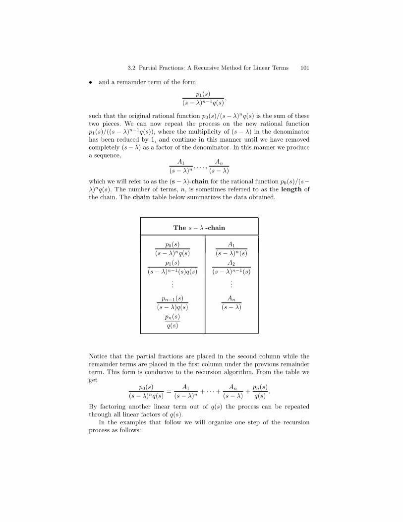
3.2 Partial Fractions: A Recursive Method for Linear Terms 101
• and a remainder term of the form
p1(s)
(s− λ)n−1q(s),
such that the original rational function p0(s)/(s−λ)nq(s) is the sum of thesetwo pieces. We can now repeat the process on the new rational functionp1(s)/((s − λ)n−1q(s)), where the multiplicity of (s − λ) in the denominatorhas been reduced by 1, and continue in this manner until we have removedcompletely (s−λ) as a factor of the denominator. In this manner we producea sequence,
A1
(s− λ)n, . . . ,
An
(s− λ)which we will refer to as the (s− λ)-chain for the rational function p0(s)/(s−λ)nq(s). The number of terms, n, is sometimes referred to as the length ofthe chain. The chain table below summarizes the data obtained.
The s− λ -chain
p0(s)
(s− λ)nq(s)
A1
(s− λ)n(s)
p1(s)
(s− λ)n−1(s)q(s)
A2
(s− λ)n−1(s)
......
pn−1(s)
(s− λ)q(s)An
(s− λ)pn(s)
q(s)
Notice that the partial fractions are placed in the second column while theremainder terms are placed in the first column under the previous remainderterm. This form is conducive to the recursion algorithm. From the table weget
p0(s)
(s− λ)nq(s)=
A1
(s− λ)n+ · · ·+ An
(s− λ) +pn(s)
q(s).
By factoring another linear term out of q(s) the process can be repeatedthrough all linear factors of q(s).
In the examples that follow we will organize one step of the recursionprocess as follows:
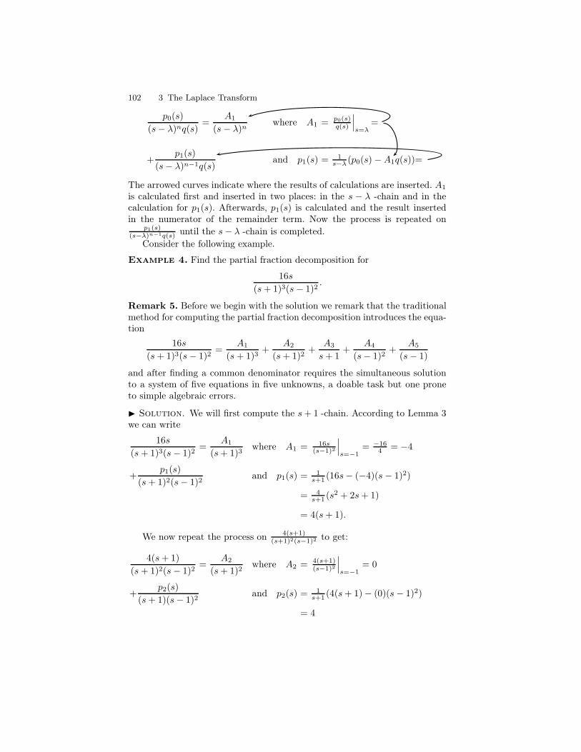
102 3 The Laplace Transform
p0(s)
(s− λ)nq(s)=
A1
(s− λ)nwhere A1 = p0(s)
q(s)
∣
∣
∣
s=λ=
+p1(s)
(s− λ)n−1q(s)and p1(s) = 1
s−λ (p0(s)−A1q(s))=
The arrowed curves indicate where the results of calculations are inserted. A1
is calculated first and inserted in two places: in the s − λ -chain and in thecalculation for p1(s). Afterwards, p1(s) is calculated and the result insertedin the numerator of the remainder term. Now the process is repeated on
p1(s)(s−λ)n−1q(s) until the s− λ -chain is completed.
Consider the following example.
Example 4. Find the partial fraction decomposition for
16s
(s+ 1)3(s− 1)2.
Remark 5. Before we begin with the solution we remark that the traditionalmethod for computing the partial fraction decomposition introduces the equa-tion
16s
(s+ 1)3(s− 1)2=
A1
(s+ 1)3+
A2
(s+ 1)2+
A3
s+ 1+
A4
(s− 1)2+
A5
(s− 1)
and after finding a common denominator requires the simultaneous solutionto a system of five equations in five unknowns, a doable task but one proneto simple algebraic errors.
I Solution. We will first compute the s+ 1 -chain. According to Lemma 3we can write
16s
(s+ 1)3(s− 1)2=
A1
(s+ 1)3where A1 = 16s
(s−1)2
∣
∣
∣
s=−1= −16
4 = −4
+p1(s)
(s+ 1)2(s− 1)2and p1(s) = 1
s+1 (16s− (−4)(s− 1)2)
= 4s+1 (s2 + 2s+ 1)
= 4(s+ 1).
We now repeat the process on 4(s+1)(s+1)2(s−1)2 to get:
4(s+ 1)
(s+ 1)2(s− 1)2=
A2
(s+ 1)2where A2 = 4(s+1)
(s−1)2
∣
∣
∣
s=−1= 0
+p2(s)
(s+ 1)(s− 1)2and p2(s) = 1
s+1 (4(s+ 1)− (0)(s− 1)2)
= 4
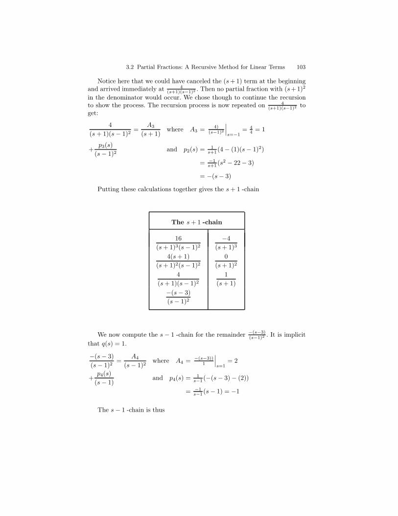
3.2 Partial Fractions: A Recursive Method for Linear Terms 103
Notice here that we could have canceled the (s+1) term at the beginningand arrived immediately at 4
(s+1)(s−1)2 . Then no partial fraction with (s+1)2
in the denominator would occur. We chose though to continue the recursionto show the process. The recursion process is now repeated on 4
(s+1)(s−1)2 toget:
4
(s+ 1)(s− 1)2=
A3
(s+ 1)where A3 = 4)
(s−1)2
∣
∣
∣
s=−1= 4
4 = 1
+p3(s)
(s− 1)2and p2(s) = 1
s+1 (4− (1)(s− 1)2)
= −1s+1 (s2 − 22− 3)
= −(s− 3)
Putting these calculations together gives the s+ 1 -chain
The s+ 1 -chain
16
(s+ 1)3(s− 1)2−4
(s+ 1)3
4(s+ 1)
(s+ 1)2(s− 1)20
(s+ 1)2
4
(s+ 1)(s− 1)21
(s+ 1)
−(s− 3)
(s− 1)2
We now compute the s− 1 -chain for the remainder −(s−3)(s−1)2 . It is implicit
that q(s) = 1.
−(s− 3)
(s− 1)2=
A4
(s− 1)2where A4 = −(s−3))
1
∣
∣
∣
s=1= 2
+p4(s)
(s− 1)and p4(s) = 1
s−1 (−(s− 3)− (2))
= −1s−1 (s− 1) = −1
The s− 1 -chain is thus
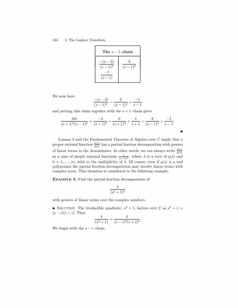
104 3 The Laplace Transform
The s− 1 -chain
−(s− 3)
(s− 1)22
(s− 1)2
−1
(s− 1)
We now have−(s− 3)
(s− 1)2=
2
(s− 1)2+−1
s− 1
and putting this chain together with the s+ 1 -chain gives
16s
(s+ 1)3(s− 1)2=
−4
(s+ 1)3+
0
(s+ 1)2+
1
s+ 1+
2
(s− 1)2+−1
s− 1.
J
Lemma 3 and the Fundamental Theorem of Algebra over C imply that aproper rational function p(s)
q(s) has a partial fraction decomposition with powers
of linear terms in the denominator. In other words, we can always write p(s)q(s)
as a sum of simple rational functions 1(s−λ)k , where λ is a root of q(s) and
k = 1, . . . ,m, with m the multiplicity of λ. Of course, even if q(s) is a realpolynomial the partial fraction decomposition may involve linear terms withcomplex roots. This situation is considered in the following example.
Example 6. Find the partial fraction decomposition of
4
(s2 + 1)2
with powers of linear terms over the complex numbers.
I Solution. The irreducible quadratic, s2 + 1, factors over C as s2 + 1 =(s− i)(s+ i). Thus
4
(s2 + 1)=
4
(s− i)2(s+ i)2.
We begin with the s− i -chain.
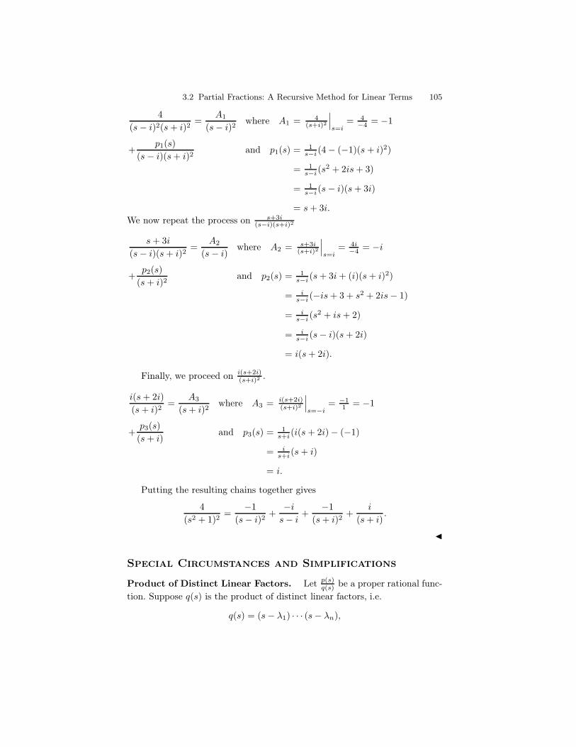
3.2 Partial Fractions: A Recursive Method for Linear Terms 105
4
(s− i)2(s+ i)2=
A1
(s− i)2 where A1 = 4(s+i)2
∣
∣
∣
s=i= 4
−4 = −1
+p1(s)
(s− i)(s+ i)2and p1(s) = 1
s−i(4− (−1)(s+ i)2)
= 1s−i(s
2 + 2is+ 3)
= 1s−i(s− i)(s+ 3i)
= s+ 3i.
We now repeat the process on s+3i(s−i)(s+i)2
s+ 3i
(s− i)(s+ i)2=
A2
(s− i) where A2 = s+3i(s+i)2
∣
∣
∣
s=i= 4i
−4 = −i
+p2(s)
(s+ i)2and p2(s) = 1
s−i (s+ 3i+ (i)(s+ i)2)
= is−i (−is+ 3 + s2 + 2is− 1)
= is−i (s
2 + is+ 2)
= is−i (s− i)(s+ 2i)
= i(s+ 2i).
Finally, we proceed on i(s+2i)(s+i)2 .
i(s+ 2i)
(s+ i)2=
A3
(s+ i)2where A3 = i(s+2i)
(s+i)2
∣
∣
∣
s=−i= −1
1 = −1
+p3(s)
(s+ i)and p3(s) = 1
s+i(i(s+ 2i)− (−1)
= is+i(s+ i)
= i.
Putting the resulting chains together gives
4
(s2 + 1)2=
−1
(s− i)2 +−is− i +
−1
(s+ i)2+
i
(s+ i).
J
Special Circumstances and Simplifications
Product of Distinct Linear Factors. Let p(s)q(s) be a proper rational func-
tion. Suppose q(s) is the product of distinct linear factors, i.e.
q(s) = (s− λ1) · · · (s− λn),
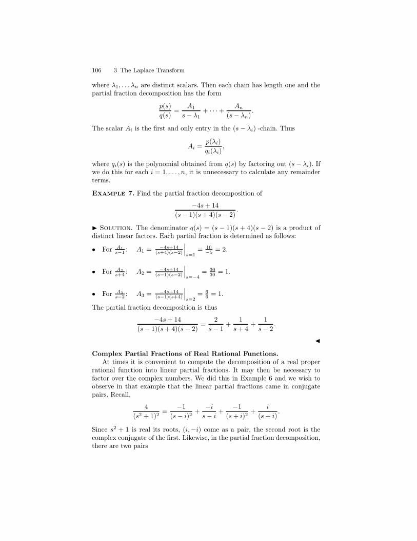
106 3 The Laplace Transform
where λ1, . . . λn are distinct scalars. Then each chain has length one and thepartial fraction decomposition has the form
p(s)
q(s)=
A1
s− λ1+ · · ·+ An
(s− λn).
The scalar Ai is the first and only entry in the (s− λi) -chain. Thus
Ai =p(λi)
qi(λi),
where qi(s) is the polynomial obtained from q(s) by factoring out (s− λi). Ifwe do this for each i = 1, . . . , n, it is unnecessary to calculate any remainderterms.
Example 7. Find the partial fraction decomposition of
−4s+ 14
(s− 1)(s+ 4)(s− 2).
I Solution. The denominator q(s) = (s − 1)(s + 4)(s − 2) is a product ofdistinct linear factors. Each partial fraction is determined as follows:
• For A1
s−1 : A1 = −4s+14(s+4)(s−2)
∣
∣
∣
s=1= 10
−5 = 2.
• For A2
s+4 : A2 = −4s+14(s−1)(s−2)
∣
∣
∣
s=−4= 30
30 = 1.
• For A3
s−2 : A3 = −4s+14(s−1)(s+4)
∣
∣
∣
s=2= 6
6 = 1.
The partial fraction decomposition is thus
−4s+ 14
(s− 1)(s+ 4)(s− 2)=
2
s− 1+
1
s+ 4+
1
s− 2.
J
Complex Partial Fractions of Real Rational Functions.At times it is convenient to compute the decomposition of a real proper
rational function into linear partial fractions. It may then be necessary tofactor over the complex numbers. We did this in Example 6 and we wish toobserve in that example that the linear partial fractions came in conjugatepairs. Recall,
4
(s2 + 1)2=
−1
(s− i)2 +−is− i +
−1
(s+ i)2+
i
(s+ i).
Since s2 + 1 is real its roots, (i,−i) come as a pair, the second root is thecomplex conjugate of the first. Likewise, in the partial fraction decomposition,there are two pairs
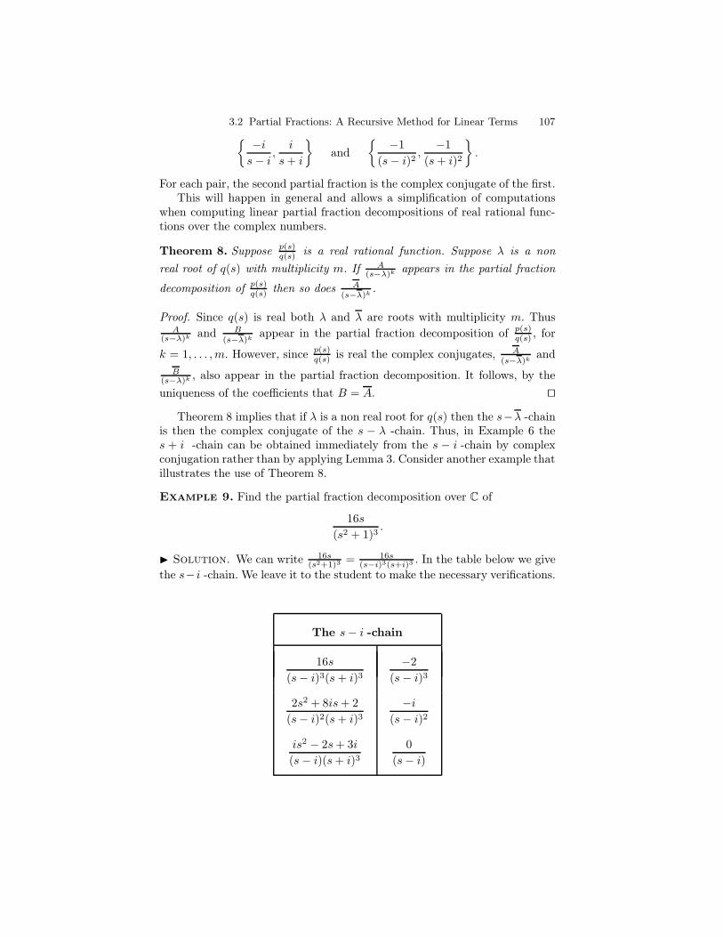
3.2 Partial Fractions: A Recursive Method for Linear Terms 107 −is− i ,
i
s+ i
and
−1
(s− i)2 ,−1
(s+ i)2
.
For each pair, the second partial fraction is the complex conjugate of the first.This will happen in general and allows a simplification of computations
when computing linear partial fraction decompositions of real rational func-tions over the complex numbers.
Theorem 8. Suppose p(s)q(s) is a real rational function. Suppose λ is a non
real root of q(s) with multiplicity m. If A(s−λ)k appears in the partial fraction
decomposition of p(s)q(s) then so does A
(s−λ)k.
Proof. Since q(s) is real both λ and λ are roots with multiplicity m. ThusA
(s−λ)k and B(s−λ)k
appear in the partial fraction decomposition of p(s)q(s) , for
k = 1, . . . ,m. However, since p(s)q(s) is real the complex conjugates, A
(s−λ)kand
B(s−λ)k , also appear in the partial fraction decomposition. It follows, by the
uniqueness of the coefficients that B = A. ut
Theorem 8 implies that if λ is a non real root for q(s) then the s−λ -chainis then the complex conjugate of the s − λ -chain. Thus, in Example 6 thes + i -chain can be obtained immediately from the s − i -chain by complexconjugation rather than by applying Lemma 3. Consider another example thatillustrates the use of Theorem 8.
Example 9. Find the partial fraction decomposition over C of
16s
(s2 + 1)3.
I Solution. We can write 16s(s2+1)3 = 16s
(s−i)3(s+i)3 . In the table below we givethe s− i -chain. We leave it to the student to make the necessary verifications.
The s− i -chain
16s
(s− i)3(s+ i)3−2
(s− i)3
2s2 + 8is+ 2
(s− i)2(s+ i)3−i
(s− i)2
is2 − 2s+ 3i
(s− i)(s+ i)30
(s− i)
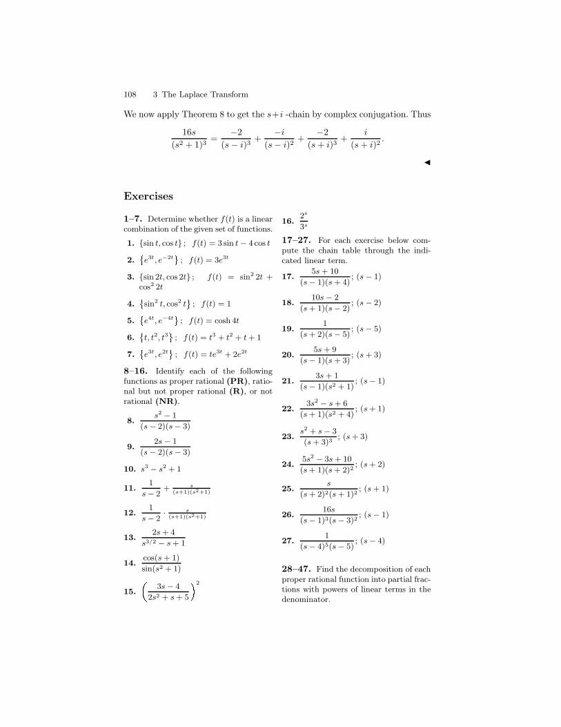
108 3 The Laplace Transform
We now apply Theorem 8 to get the s+i -chain by complex conjugation. Thus
16s
(s2 + 1)3=
−2
(s− i)3 +−i
(s− i)2 +−2
(s+ i)3+
i
(s+ i)2.
J
Exercises
1–7. Determine whether f(t) is a linearcombination of the given set of functions.
1. sin t, cos t ; f(t) = 3 sin t − 4 cos t
2. e3t, e−2t ; f(t) = 3e3t
3. sin 2t, cos 2t ; f(t) = sin2 2t +cos2 2t
4. sin2 t, cos2 t; f(t) = 1
5. e4t, e−4t ; f(t) = cosh 4t
6. t, t2, t3; f(t) = t3 + t2 + t + 1
7. e3t, e2t ; f(t) = te3t + 2e2t
8–16. Identify each of the followingfunctions as proper rational (PR), ratio-nal but not proper rational (R), or notrational (NR).
8.s2 − 1
(s − 2)(s − 3)
9.2s − 1
(s − 2)(s − 3)
10. s3 − s2 + 1
11.1
s − 2+ s
(s+1)(s2+1)
12.1
s − 2· s
(s+1)(s2+1)
13.2s + 4
s3/2 − s + 1
14.cos(s + 1)
sin(s2 + 1)
15. 3s − 4
2s2 + s + 52
16.2s
3s
17–27. For each exercise below com-pute the chain table through the indi-cated linear term.
17.5s + 10
(s − 1)(s + 4); (s − 1)
18.10s − 2
(s + 1)(s − 2); (s − 2)
19.1
(s + 2)(s − 5); (s − 5)
20.5s + 9
(s − 1)(s + 3); (s + 3)
21.3s + 1
(s − 1)(s2 + 1); (s − 1)
22.3s2 − s + 6
(s + 1)(s2 + 4); (s + 1)
23.s2 + s − 3
(s + 3)3; (s + 3)
24.5s2 − 3s + 10
(s + 1)(s + 2)2; (s + 2)
25.s
(s + 2)2(s + 1)2; (s + 1)
26.16s
(s − 1)3(s − 3)2; (s − 1)
27.1
(s − 4)5(s − 5); (s − 4)
28–47. Find the decomposition of eachproper rational function into partial frac-tions with powers of linear terms in thedenominator.
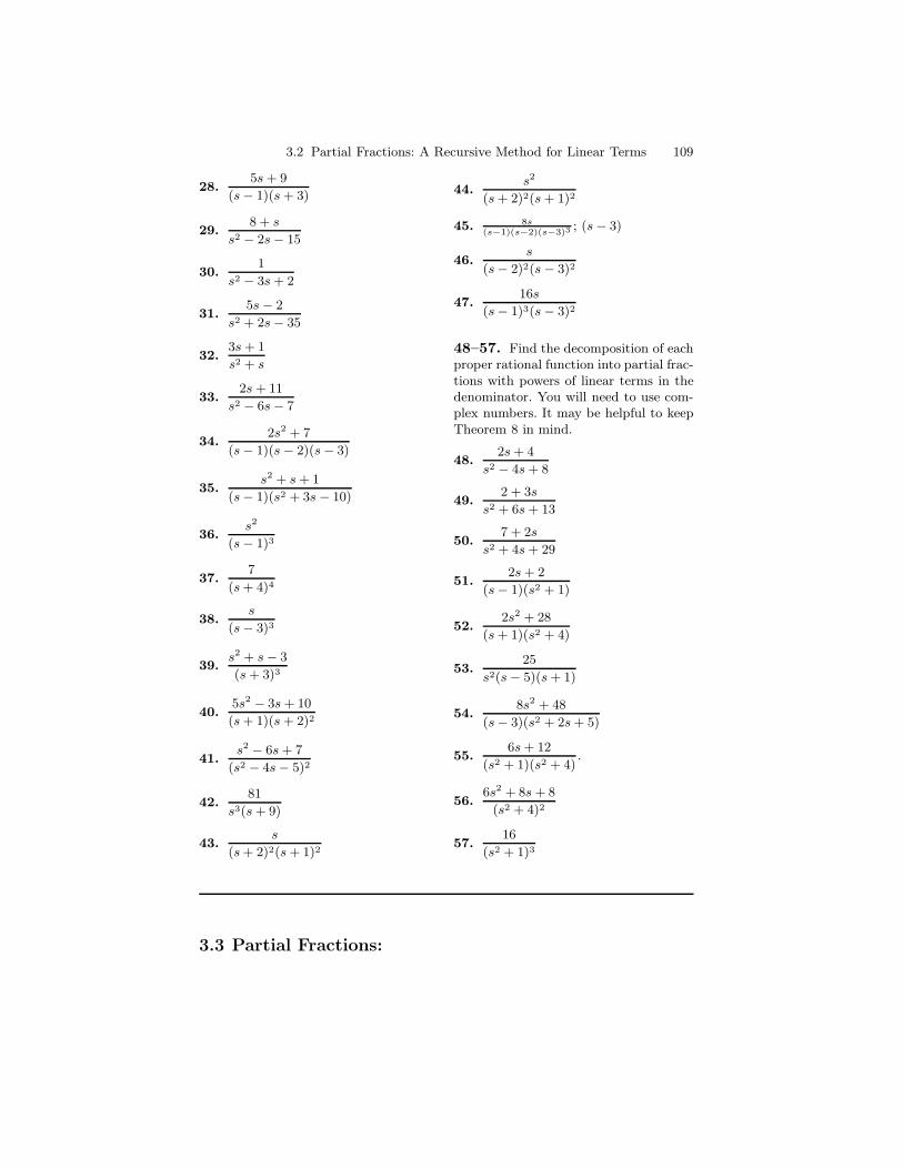
3.2 Partial Fractions: A Recursive Method for Linear Terms 109
28.5s + 9
(s − 1)(s + 3)
29.8 + s
s2 − 2s − 15
30.1
s2 − 3s + 2
31.5s − 2
s2 + 2s − 35
32.3s + 1
s2 + s
33.2s + 11
s2 − 6s − 7
34.2s2 + 7
(s − 1)(s − 2)(s − 3)
35.s2 + s + 1
(s − 1)(s2 + 3s − 10)
36.s2
(s − 1)3
37.7
(s + 4)4
38.s
(s − 3)3
39.s2 + s − 3
(s + 3)3
40.5s2 − 3s + 10
(s + 1)(s + 2)2
41.s2 − 6s + 7
(s2 − 4s − 5)2
42.81
s3(s + 9)
43.s
(s + 2)2(s + 1)2
44.s2
(s + 2)2(s + 1)2
45. 8s(s−1)(s−2)(s−3)3
; (s − 3)
46.s
(s − 2)2(s − 3)2
47.16s
(s − 1)3(s − 3)2
48–57. Find the decomposition of eachproper rational function into partial frac-tions with powers of linear terms in thedenominator. You will need to use com-plex numbers. It may be helpful to keepTheorem 8 in mind.
48.2s + 4
s2 − 4s + 8
49.2 + 3s
s2 + 6s + 13
50.7 + 2s
s2 + 4s + 29
51.2s + 2
(s − 1)(s2 + 1)
52.2s2 + 28
(s + 1)(s2 + 4)
53.25
s2(s − 5)(s + 1)
54.8s2 + 48
(s − 3)(s2 + 2s + 5)
55.6s + 12
(s2 + 1)(s2 + 4).
56.6s2 + 8s + 8
(s2 + 4)2
57.16
(s2 + 1)3
3.3 Partial Fractions:
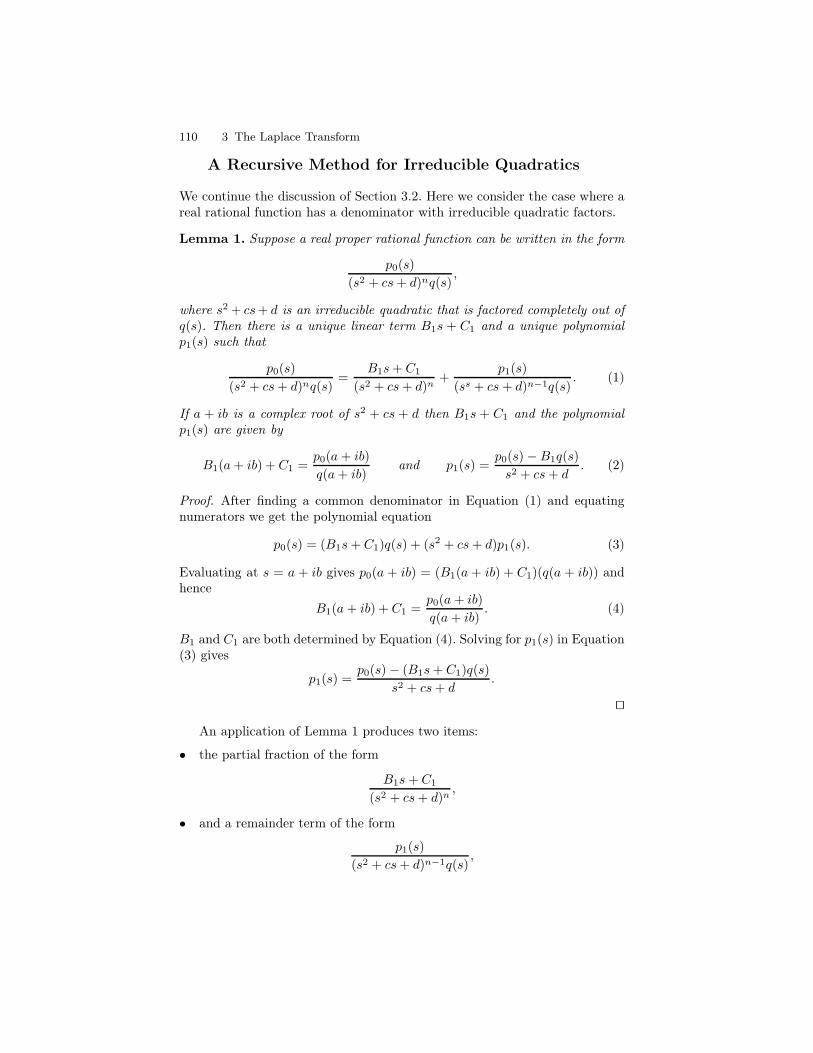
110 3 The Laplace Transform
A Recursive Method for Irreducible Quadratics
We continue the discussion of Section 3.2. Here we consider the case where areal rational function has a denominator with irreducible quadratic factors.
Lemma 1. Suppose a real proper rational function can be written in the form
p0(s)
(s2 + cs+ d)nq(s),
where s2 + cs+ d is an irreducible quadratic that is factored completely out ofq(s). Then there is a unique linear term B1s + C1 and a unique polynomialp1(s) such that
p0(s)
(s2 + cs+ d)nq(s)=
B1s+ C1
(s2 + cs+ d)n+
p1(s)
(ss + cs+ d)n−1q(s). (1)
If a + ib is a complex root of s2 + cs + d then B1s + C1 and the polynomialp1(s) are given by
B1(a+ ib) + C1 =p0(a+ ib)
q(a+ ib)and p1(s) =
p0(s)−B1q(s)
s2 + cs+ d. (2)
Proof. After finding a common denominator in Equation (1) and equatingnumerators we get the polynomial equation
p0(s) = (B1s+ C1)q(s) + (s2 + cs+ d)p1(s). (3)
Evaluating at s = a+ ib gives p0(a + ib) = (B1(a + ib) + C1)(q(a + ib)) andhence
B1(a+ ib) + C1 =p0(a+ ib)
q(a+ ib). (4)
B1 and C1 are both determined by Equation (4). Solving for p1(s) in Equation(3) gives
p1(s) =p0(s)− (B1s+ C1)q(s)
s2 + cs+ d.
ut
An application of Lemma 1 produces two items:
• the partial fraction of the form
B1s+ C1
(s2 + cs+ d)n,
• and a remainder term of the form
p1(s)
(s2 + cs+ d)n−1q(s),
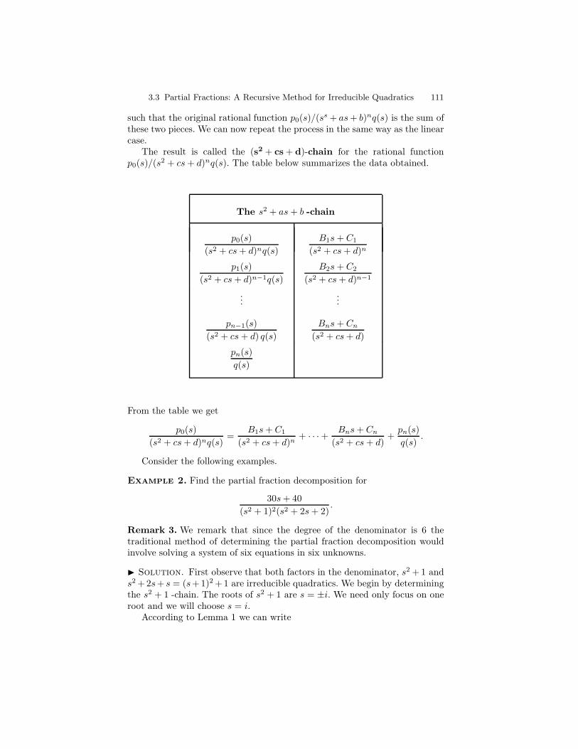
3.3 Partial Fractions: A Recursive Method for Irreducible Quadratics 111
such that the original rational function p0(s)/(ss + as+ b)nq(s) is the sum of
these two pieces. We can now repeat the process in the same way as the linearcase.
The result is called the (s2 + cs + d)-chain for the rational functionp0(s)/(s
2 + cs+ d)nq(s). The table below summarizes the data obtained.
The s2 + as+ b -chain
p0(s)
(s2 + cs+ d)nq(s)
B1s+ C1
(s2 + cs+ d)n
p1(s)
(s2 + cs+ d)n−1q(s)
B2s+ C2
(s2 + cs+ d)n−1
......
pn−1(s)
(s2 + cs+ d) q(s)
Bns+ Cn
(s2 + cs+ d)
pn(s)
q(s)
From the table we get
p0(s)
(s2 + cs+ d)nq(s)=
B1s+ C1
(s2 + cs+ d)n+ · · ·+ Bns+ Cn
(s2 + cs+ d)+pn(s)
q(s).
Consider the following examples.
Example 2. Find the partial fraction decomposition for
30s+ 40
(s2 + 1)2(s2 + 2s+ 2).
Remark 3. We remark that since the degree of the denominator is 6 thetraditional method of determining the partial fraction decomposition wouldinvolve solving a system of six equations in six unknowns.
I Solution. First observe that both factors in the denominator, s2 + 1 ands2 +2s+ s = (s+1)2 +1 are irreducible quadratics. We begin by determiningthe s2 + 1 -chain. The roots of s2 + 1 are s = ±i. We need only focus on oneroot and we will choose s = i.
According to Lemma 1 we can write
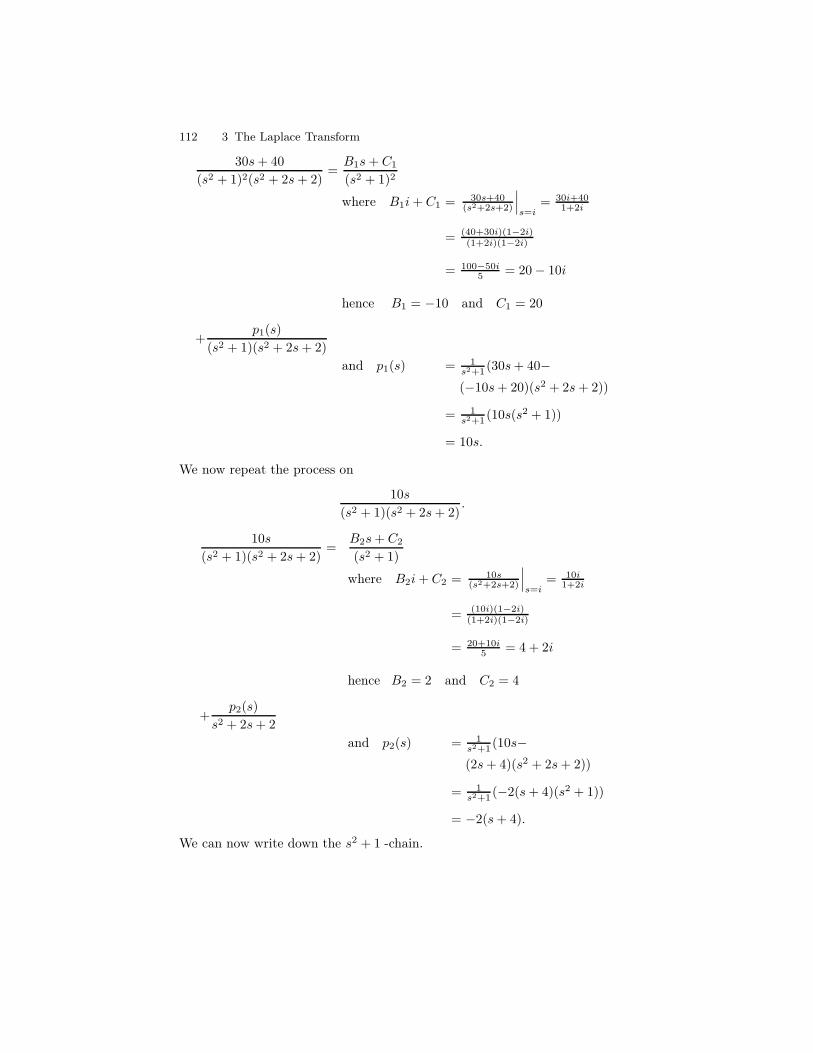
112 3 The Laplace Transform
30s+ 40
(s2 + 1)2(s2 + 2s+ 2)=B1s+ C1
(s2 + 1)2
where B1i+ C1 = 30s+40(s2+2s+2)
∣
∣
∣
s=i= 30i+40
1+2i
= (40+30i)(1−2i)(1+2i)(1−2i)
= 100−50i5 = 20− 10i
hence B1 = −10 and C1 = 20
+p1(s)
(s2 + 1)(s2 + 2s+ 2)
and p1(s) = 1s2+1 (30s+ 40−(−10s+ 20)(s2 + 2s+ 2))
= 1s2+1 (10s(s2 + 1))
= 10s.
We now repeat the process on
10s
(s2 + 1)(s2 + 2s+ 2).
10s
(s2 + 1)(s2 + 2s+ 2)=
B2s+ C2
(s2 + 1)
where B2i+ C2 = 10s(s2+2s+2)
∣
∣
∣
s=i= 10i
1+2i
= (10i)(1−2i)(1+2i)(1−2i)
= 20+10i5 = 4 + 2i
hence B2 = 2 and C2 = 4
+p2(s)
s2 + 2s+ 2
and p2(s) = 1s2+1 (10s−(2s+ 4)(s2 + 2s+ 2))
= 1s2+1 (−2(s+ 4)(s2 + 1))
= −2(s+ 4).
We can now write down the s2 + 1 -chain.
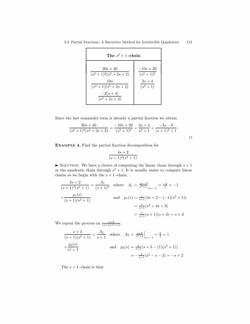
3.3 Partial Fractions: A Recursive Method for Irreducible Quadratics 113
The s2 + 1 -chain
30s+ 40
(s2 + 1)2(s2 + 2s+ 2)
−10s+ 20
(s2 + 1)2
10s
(s2 + 1)(s2 + 2s+ 2)
2s+ 4
(s2 + 1)
−2(s+ 4)
(s2 + 2s+ 2)
Since the last remainder term is already a partial fraction we obtain
30s+ 40
(s2 + 1)2(s2 + 2s+ 2)=−10s+ 20
(s2 + 1)2+
2s+ 4
s2 + 1+−2s− 8
(s+ 1)2 + 1.
utExample 4. Find the partial fraction decomposition for
4s+ 2
(s+ 1)2(s2 + 1).
I Solution. We have a choice of computing the linear chain through s+ 1or the quadratic chain through s2 + 1. It is usually easier to compute linearchains so we begin with the s+ 1 -chain.
4s+ 2
(s+ 1)2(s2 + 1)=
A1
(s+ 1)2where A1 = 4s+2
s2+1
∣
∣
∣
s=−1= −2
2 = −1
+p1(s)
(s+ 1)(s2 + 1)and p1(s) = 1
s+1 (4s+ 2− (−1)(s2 + 1))
= 1s+1 (s2 + 4s+ 3)
= 1s+1 (s+ 1)(s+ 3) = s+ 3
We repeat the process on s+3(s+1)(s2+1) .
s+ 3
(s+ 1)(s2 + 1)=
A2
s+ 1where A2 = s+3
s2+1
∣
∣
∣
s=−1= 2
2 = 1
+p2(s)
s2 + 1and p2(s) = 1
s+1 (s+ 3− (1)(s2 + 1))
= − 1s+1 (s2 − s− 2) = −s+ 2
The s+ 1 -chain is thus
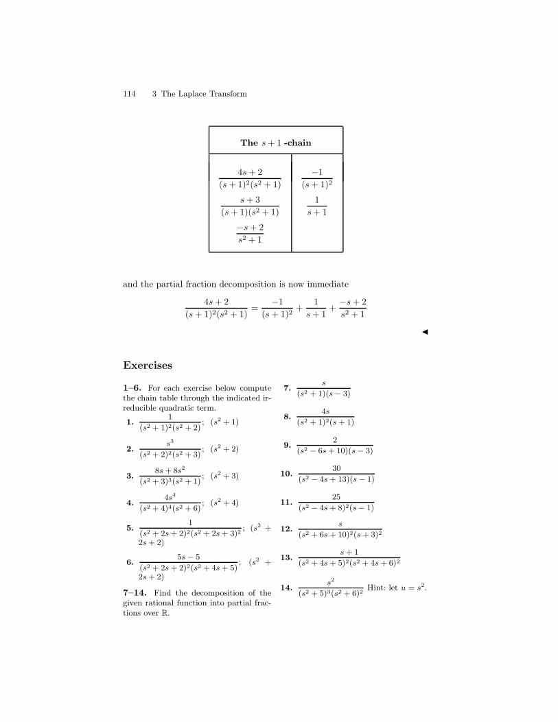
114 3 The Laplace Transform
The s+ 1 -chain
4s+ 2
(s+ 1)2(s2 + 1)
−1
(s+ 1)2
s+ 3
(s+ 1)(s2 + 1)
1
s+ 1
−s+ 2
s2 + 1
and the partial fraction decomposition is now immediate
4s+ 2
(s+ 1)2(s2 + 1)=
−1
(s+ 1)2+
1
s+ 1+−s+ 2
s2 + 1
J
Exercises
1–6. For each exercise below computethe chain table through the indicated ir-reducible quadratic term.
1.1
(s2 + 1)2(s2 + 2); (s2 + 1)
2.s3
(s2 + 2)2(s2 + 3); (s2 + 2)
3.8s + 8s2
(s2 + 3)3(s2 + 1); (s2 + 3)
4.4s4
(s2 + 4)4(s2 + 6); (s2 + 4)
5.1
(s2 + 2s + 2)2(s2 + 2s + 3)2; (s2 +
2s + 2)
6.5s − 5
(s2 + 2s + 2)2(s2 + 4s + 5); (s2 +
2s + 2)
7–14. Find the decomposition of thegiven rational function into partial frac-tions over R.
7.s
(s2 + 1)(s − 3)
8.4s
(s2 + 1)2(s + 1)
9.2
(s2 − 6s + 10)(s − 3)
10.30
(s2 − 4s + 13)(s − 1)
11.25
(s2 − 4s + 8)2(s − 1)
12.s
(s2 + 6s + 10)2(s + 3)2
13.s + 1
(s2 + 4s + 5)2(s2 + 4s + 6)2
14.s2
(s2 + 5)3(s2 + 6)2Hint: let u = s2.
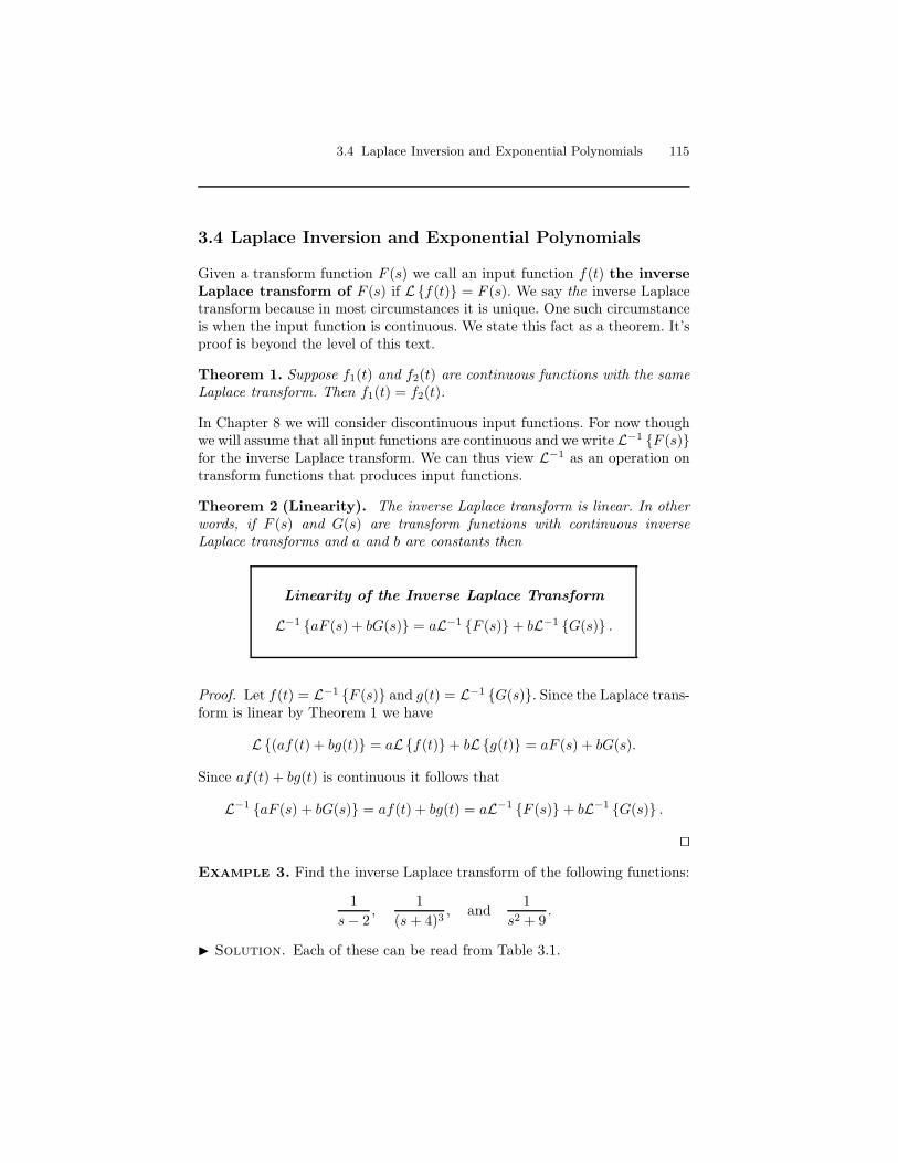
3.4 Laplace Inversion and Exponential Polynomials 115
3.4 Laplace Inversion and Exponential Polynomials
Given a transform function F (s) we call an input function f(t) the inverseLaplace transform of F (s) if Lf(t) = F (s). We say the inverse Laplacetransform because in most circumstances it is unique. One such circumstanceis when the input function is continuous. We state this fact as a theorem. It’sproof is beyond the level of this text.
Theorem 1. Suppose f1(t) and f2(t) are continuous functions with the sameLaplace transform. Then f1(t) = f2(t).
In Chapter 8 we will consider discontinuous input functions. For now thoughwe will assume that all input functions are continuous and we write L−1 F (s)for the inverse Laplace transform. We can thus view L−1 as an operation ontransform functions that produces input functions.
Theorem 2 (Linearity). The inverse Laplace transform is linear. In otherwords, if F (s) and G(s) are transform functions with continuous inverseLaplace transforms and a and b are constants then
Linearity of the Inverse Laplace Transform
L−1 aF (s) + bG(s) = aL−1 F (s)+ bL−1 G(s) .
Proof. Let f(t) = L−1 F (s) and g(t) = L−1 G(s). Since the Laplace trans-form is linear by Theorem 1 we have
L(af(t) + bg(t) = aLf(t)+ bLg(t) = aF (s) + bG(s).
Since af(t) + bg(t) is continuous it follows that
L−1 aF (s) + bG(s) = af(t) + bg(t) = aL−1 F (s) + bL−1 G(s) .
ut
Example 3. Find the inverse Laplace transform of the following functions:
1
s− 2,
1
(s+ 4)3, and
1
s2 + 9.
I Solution. Each of these can be read from Table 3.1.
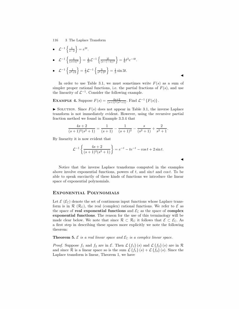
116 3 The Laplace Transform
• L−1
1s−2
= e2t.
• L−1
1(s+4)3
= 13!L−1
3!(s−(−4))3
= 16 t
2e−4t.
• L−1
1s2+9
= 13L−1
3s2+32
= 13 sin 3t.
J
In order to use Table 3.1, we must sometimes write F (s) as a sum ofsimpler proper rational functions, i.e. the partial fractions of F (s), and usethe linearity of L−1. Consider the following example.
Example 4. Suppose F (s) = 4s+2(s+1)2(s2+1) . Find L−1 F (s) .
I Solution. Since F (s) does not appear in Table 3.1, the inverse Laplacetransform is not immediately evident. However, using the recursive partialfraction method we found in Example 3.3.4 that
4s+ 2
(s+ 1)2(s2 + 1)=
1
(s+ 1)− 1
(s+ 1)2− s
(s2 + 1)+
2
s2 + 1.
By linearity it is now evident that
L−1
4s+ 2
(s+ 1)2(s2 + 1)
= e−t − te−t − cos t+ 2 sin t.
J
Notice that the inverse Laplace transforms computed in the examplesabove involve exponential functions, powers of t, and sin t and cos t. To beable to speak succinctly of these kinds of functions we introduce the linearspace of exponential polynomials.
Exponential Polynomials
Let E (EC) denote the set of continuous input functions whose Laplace trans-form is in R (RC), the real (complex) rational functions. We refer to E asthe space of real exponential functions and EC as the space of complexexponential functions. The reason for the use of this terminology will bemade clear below. We note that since R ⊂ RC it follows that E ⊂ EC. Asa first step in describing these spaces more explicitly we note the followingtheorem:
Theorem 5. E is a real linear space and EC is a complex linear space.
Proof. Suppose f1 and f2 are in E . Then Lf1 (s) and Lf2 (s) are in Rand since R is a linear space so is the sum Lf1 (s) + Lf2 (s). Since theLaplace transform is linear, Theorem 1, we have
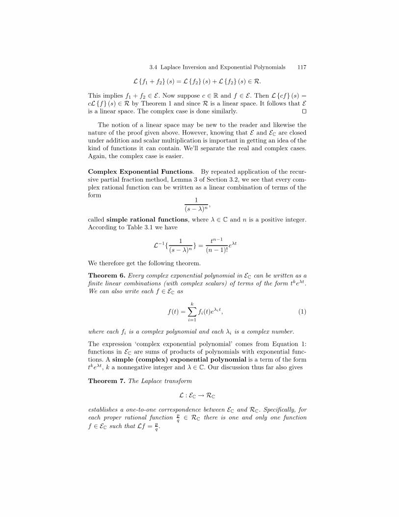
3.4 Laplace Inversion and Exponential Polynomials 117
Lf1 + f2 (s) = Lf2 (s) + Lf2 (s) ∈ R.
This implies f1 + f2 ∈ E . Now suppose c ∈ R and f ∈ E . Then Lcf (s) =cLf (s) ∈ R by Theorem 1 and since R is a linear space. It follows that Eis a linear space. The complex case is done similarly. ut
The notion of a linear space may be new to the reader and likewise thenature of the proof given above. However, knowing that E and EC are closedunder addition and scalar multiplication is important in getting an idea of thekind of functions it can contain. We’ll separate the real and complex cases.Again, the complex case is easier.
Complex Exponential Functions. By repeated application of the recur-sive partial fraction method, Lemma 3 of Section 3.2, we see that every com-plex rational function can be written as a linear combination of terms of theform
1
(s− λ)n,
called simple rational functions, where λ ∈ C and n is a positive integer.According to Table 3.1 we have
L−1 1
(s− λ)n =
tn−1
(n− 1)!eλt
We therefore get the following theorem.
Theorem 6. Every complex exponential polynomial in EC can be written as afinite linear combinations (with complex scalars) of terms of the form tkeλt.We can also write each f ∈ EC as
f(t) =
k∑
i=1
fi(t)eλit, (1)
where each fi is a complex polynomial and each λi is a complex number.
The expression ‘complex exponential polynomial’ comes from Equation 1:functions in EC are sums of products of polynomials with exponential func-tions. A simple (complex) exponential polynomial is a term of the formtkeλt, k a nonnegative integer and λ ∈ C. Our discussion thus far also gives
Theorem 7. The Laplace transform
L : EC →RC
establishes a one-to-one correspondence between EC and RC. Specifically, foreach proper rational function p
q ∈ RC there is one and only one function
f ∈ EC such that Lf = pq .
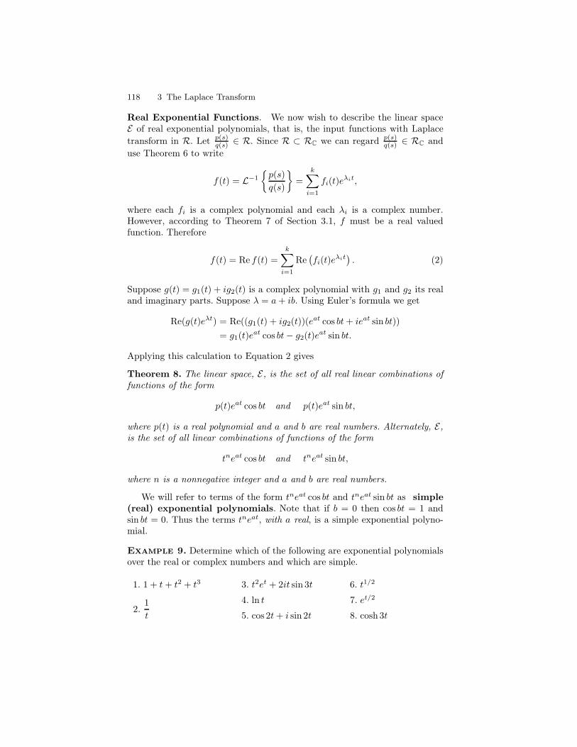
118 3 The Laplace Transform
Real Exponential Functions. We now wish to describe the linear spaceE of real exponential polynomials, that is, the input functions with Laplacetransform in R. Let p(s)
q(s) ∈ R. Since R ⊂ RC we can regard p(s)q(s) ∈ RC and
use Theorem 6 to write
f(t) = L−1
p(s)
q(s)
=
k∑
i=1
fi(t)eλit,
where each fi is a complex polynomial and each λi is a complex number.However, according to Theorem 7 of Section 3.1, f must be a real valuedfunction. Therefore
f(t) = Re f(t) =
k∑
i=1
Re(
fi(t)eλit)
. (2)
Suppose g(t) = g1(t) + ig2(t) is a complex polynomial with g1 and g2 its realand imaginary parts. Suppose λ = a+ ib. Using Euler’s formula we get
Re(g(t)eλt) = Re((g1(t) + ig2(t))(eat cos bt+ ieat sin bt))
= g1(t)eat cos bt− g2(t)eat sin bt.
Applying this calculation to Equation 2 gives
Theorem 8. The linear space, E, is the set of all real linear combinations offunctions of the form
p(t)eat cos bt and p(t)eat sin bt,
where p(t) is a real polynomial and a and b are real numbers. Alternately, E,is the set of all linear combinations of functions of the form
tneat cos bt and tneat sin bt,
where n is a nonnegative integer and a and b are real numbers.
We will refer to terms of the form tneat cos bt and tneat sin bt as simple(real) exponential polynomials. Note that if b = 0 then cos bt = 1 andsin bt = 0. Thus the terms tneat, with a real, is a simple exponential polyno-mial.
Example 9. Determine which of the following are exponential polynomialsover the real or complex numbers and which are simple.
1. 1 + t+ t2 + t3
2.1
t
3. t2et + 2it sin 3t
4. ln t
5. cos 2t+ i sin 2t
6. t1/2
7. et/2
8. cosh 3t
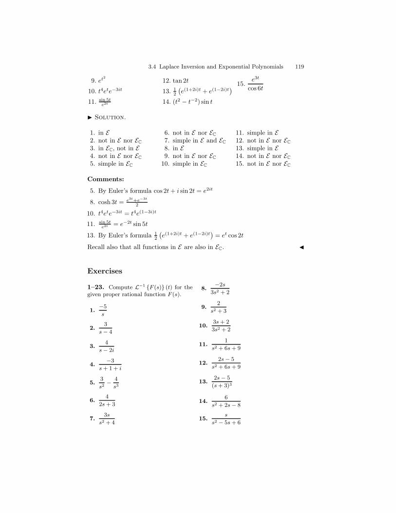
3.4 Laplace Inversion and Exponential Polynomials 119
9. et2
10. t4ete−3it
11. sin 5te2t
12. tan 2t
13. 12
(
e(1+2i)t + e(1−2i)t)
14. (t2 − t−2) sin t
15.e3t
cos 6t
I Solution.
1. in E2. not in E nor EC
3. in EC, not in E4. not in E nor EC
5. simple in EC
6. not in E nor EC
7. simple in E and EC
8. in E9. not in E nor EC
10. simple in EC
11. simple in E12. not in E nor EC
13. simple in E14. not in E nor EC
15. not in E nor EC
Comments:
5. By Euler’s formula cos 2t+ i sin 2t = e2it
8. cosh 3t = e3t+e−3t
2
10. t4ete−3it = t4e(1−3i)t
11. sin 5te2t = e−2t sin 5t
13. By Euler’s formula 12
(
e(1+2i)t + e(1−2i)t)
= et cos 2t
Recall also that all functions in E are also in EC. J
Exercises
1–23. Compute L−1 F (s) (t) for thegiven proper rational function F (s).
1.−5
s
2.3
s − 4
3.4
s − 2i
4.−3
s + 1 + i
5.3
s2− 4
s3
6.4
2s + 3
7.3s
s2 + 4
8.−2s
3s2 + 2
9.2
s2 + 3
10.3s + 2
3s2 + 2
11.1
s2 + 6s + 9
12.2s − 5
s2 + 6s + 9
13.2s − 5
(s + 3)3
14.6
s2 + 2s − 8
15.s
s2 − 5s + 6
120 3 The Laplace Transform
16.2s2 − 5s + 1
(s − 2)4
17.2s + 6
s2 − 6s + 5
18.4s2
(s − 1)2(s + 1)2
19.27
s3(s + 3)
20.8s + 16
(s2 + 4)(s − 2)2
21.5s + 15
(s2 + 9)(s − 1)
22.12
s2(s + 1)(s − 2)
23.2s
(s − 3)3(s − 4)2
24–34. Determine which of the follow-ing functions are in the linear space E ofexponential polynomials.
24. t2e−2t
25. t−2e2t
26. t/et
27. et/t
28. t sin(4t − π4)
29. (t + et)2
30. (t + et)−2
31. tet/2
32. t1/2et
33. sin 2t/e2t
34. e2t/ sin 2t
35–38. Verify the following closureproperties of the linear space of exponen-tial polynomials.
35. Multiplication. Show that if f and gare in E (EC), then so is fg.
36. Differentiation. Show that if f is inE (EC,) then so is the derivative f ′.
37. Integration. Show that if f is in E ,(EC) then so is
f(t) dt.
38. Show that E (EC) is not closed underinversion. That is, find a function fso that 1/f is not in E (EC).
3.5 Laplace Inversion involving Irreducible Quadratics
Let’s now return to our discussion about the inverse Laplace transform. Bythe recursive partial fraction method each (real or complex) rational functionp(s)q(s) can be written as a linear combination of terms of the form 1
(s−λ)k , whereλ is a (possibly complex) root of q and k is a positive integers less than orequal to the multiplicity of λ in q(s). The inversion formula
L−1
1
(s− λ)k
=tk
k!eλt. (1)
and linearity then gives a straightforward means of computing L−1 p(s)/q(s).Of course, all of this assumes that one knows the factorization of q(s).
Now, for each real rational function we would like to express its inverseLaplace transform as a linear combination of simple real exponential poly-nomials. The partial fraction decomposition for a real rational function is a
3.5 Laplace Inversion involving Irreducible Quadratics 121
linear combination of the simple real rational functions
1
(s− a)k,
1
((s− a)2 + b2)k, and
s
((s− a)2 + b2)k, (2)
where a, b are real and b > 0. The inversion of the first simple rational functionis straightforward, it is given by Equation 1 with λ = a. However, whenpowers of irreducible quadratics are involved the inversion is a little morecomplicated. To facilitate their inversion we introduce two Laplace transformtools. Applications of these tools will reduce powers of quadratics to the cases
1
(s2 + 1)kand
s
(s2 + 1)k. (3)
We will discuss how each of these can be handled later on in this section.The first tool is a new way of looking at the first translation principle for theLaplace transform. By inverting both side of the formula in Theorem 12 ofSection 3.1 we get the following equivalent theorem.
Theorem 1. Suppose F (s) is a function in transform space. Then
First Translation Principle
L−1 F (s− a) = eatL−1 F (s) .
The First Translation Principle allows us to remove the shift by a in therational functions of Equation (2) to get a linear combination of simple partialfractions of the from
1
(s2 + b2)kand
s
(s2 + b2)k. (4)
Consider the following examples where k = 1. (The case k > 1 is similar andan example of this type will be considered later in this section.)
Example 2. Find the inverse Laplace transform of
1
s2 + 6s+ 25.
I Solution. Completing the square of the denominator gives: s2+6s+25 =s2 + 6s + 9 + 25 − 9 = (s + 3)2 + 42. With a = −3 in the First TranslationPrinciple we get
L−1
1
s2 + 6s+ 25
= L−1
1
(s−−3)2 + 42
= e−3tL−1
1
s2 + 42
=1
4e−3t sin 4t.
122 3 The Laplace Transform
The third line comes directly from Table 3.1. J
Example 3. Find the inverse Laplace transform of
3s+ 2
s2 − 4s+ 7.
I Solution. Completing the square of the denominator gives s2 − 4s+ 7 =
s2 − 4s + 4 + 3 = (s − 2)2 +√
32. In order to apply the First Translation
Principle with a = 2 the numerator must also be rewritten with s translatedby 2. Thus 3s+ 2 = 3(s− 2 + 2) + 2 = 3(s− 2) + 8. We now get
L−1
3s+ 2
s2 − 4s+ 7
= L−1
3(s− 2) + 8
(s− 2)2 +√
32
= e2tL−1
3s+ 8
s2 +√
32
= e2t
(
3L−1
s
s2 +√
32
+8√3L−1
√3
s2 +√
32
)
= e2t
(
3 cos√
3t+8√3
sin√
3t
)
.
J
Notice that in each of these examples after the First Translation Principleis applied the inversions reduce to expressions of the form given in Equation(4). We now introduce a tool that reduces these simple partial fractions tothe case where b = 1.
Suppose f(t) is an function and b is a positive real number. The functiong(t) = f(bt) is called a dilation of f by b. If the domain of f includes[0,∞) then so does any dilation of f since b is positive. The following theoremdescribes the Laplace transform of a dilation.
Theorem 4. Suppose f(t) is an input function and b is a positive real number.Then
The Dilation Principle
bLf(bt)) (s) = Lf(t) ( sb ).
Proof. This result follows from the definition of the Laplace transform:
3.5 Laplace Inversion involving Irreducible Quadratics 123
bLf(bt) (s) = b
∫ ∞
0
e−stf(bt) dt
= b
∫ ∞
0
e−sbrf(r)
dr
b
= Lf(t)(s
b
)
.
To get the second line we made the change of variable t = rb . Since b > 0 the
limits of integration remain unchanged. ut
To illustrate the Dilation Principle consider the following verifications.
• For f(t) = et: bL
ebt
(s) = bs−b = 1
( sb−1) = Let
(
sb
)
.
• For f(t) = cos t: bLcos bt (s) = b2
s2+b2 = 1
(( sb )
2+1)
= Lcos t(
sb
)
.
• For f(t) = sin t: bLsin bt (s) = bss2+b2 =
sb
(( sb )
2+1)
= Lsin t(
sb
)
.
Example 5. Given that L
sin tt
= cot−1(s) determine
L
sin bt
t
(s).
I Solution. By linearity and the Dilation principle we have
L
sin bt
t
(s) = bL
sin bt
bt
(s)
= L
sin t
t
(s/b)
= cot−1(s/b).
J
We now consider an application of the Dilation Principle that reducesEquation (4) to Equation (3).
Proposition 6. Set A(t) = L−1
1(s2+1)k+1
and B(t) = L−1
s(s2+1)k+1
.
Then
L−1
b
(s2 + b2)k+1
(t) =1
b2kA(bt)
L−1
s
(s2 + b2)k+1
(t) =1
b2kB(bt)
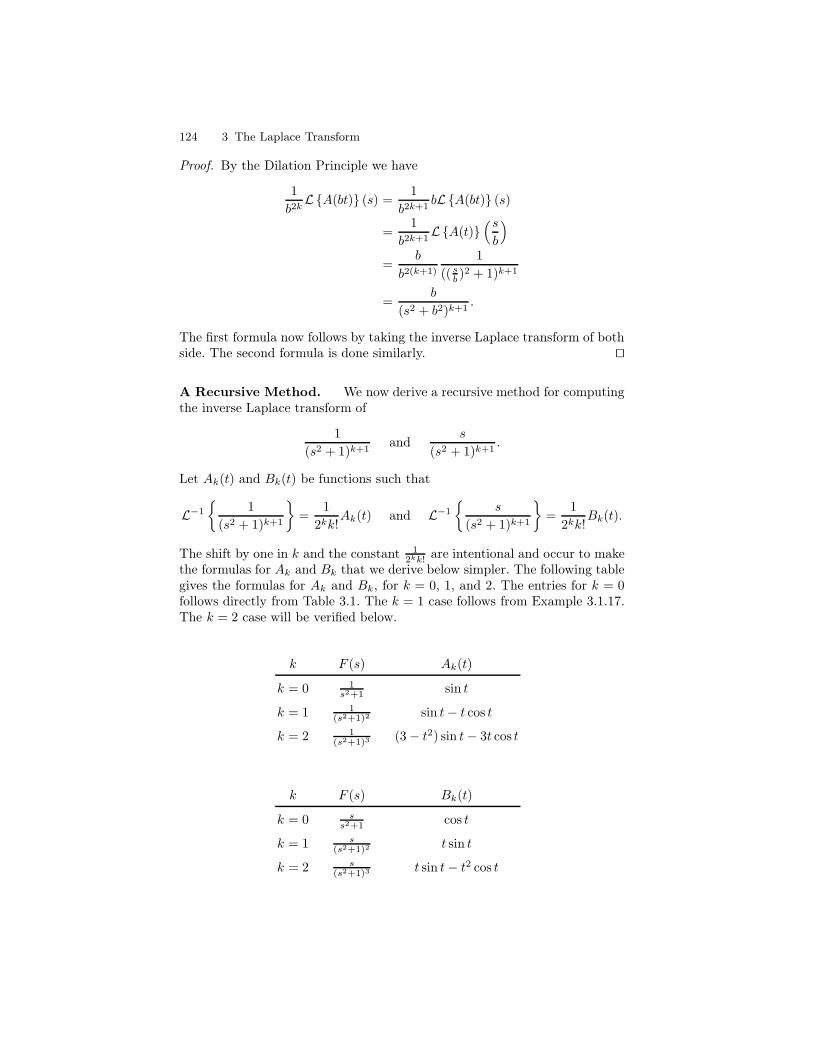
124 3 The Laplace Transform
Proof. By the Dilation Principle we have
1
b2kLA(bt) (s) =
1
b2k+1bLA(bt) (s)
=1
b2k+1LA(t)
(s
b
)
=b
b2(k+1)
1
(( sb )2 + 1)k+1
=b
(s2 + b2)k+1.
The first formula now follows by taking the inverse Laplace transform of bothside. The second formula is done similarly. ut
A Recursive Method. We now derive a recursive method for computingthe inverse Laplace transform of
1
(s2 + 1)k+1and
s
(s2 + 1)k+1.
Let Ak(t) and Bk(t) be functions such that
L−1
1
(s2 + 1)k+1
=1
2kk!Ak(t) and L−1
s
(s2 + 1)k+1
=1
2kk!Bk(t).
The shift by one in k and the constant 12kk! are intentional and occur to make
the formulas for Ak and Bk that we derive below simpler. The following tablegives the formulas for Ak and Bk, for k = 0, 1, and 2. The entries for k = 0follows directly from Table 3.1. The k = 1 case follows from Example 3.1.17.The k = 2 case will be verified below.
k F (s) Ak(t)
k = 0 1s2+1 sin t
k = 1 1(s2+1)2 sin t− t cos t
k = 2 1(s2+1)3 (3− t2) sin t− 3t cos t
k F (s) Bk(t)
k = 0 ss2+1 cos t
k = 1 s(s2+1)2 t sin t
k = 2 s(s2+1)3 t sin t− t2 cos t
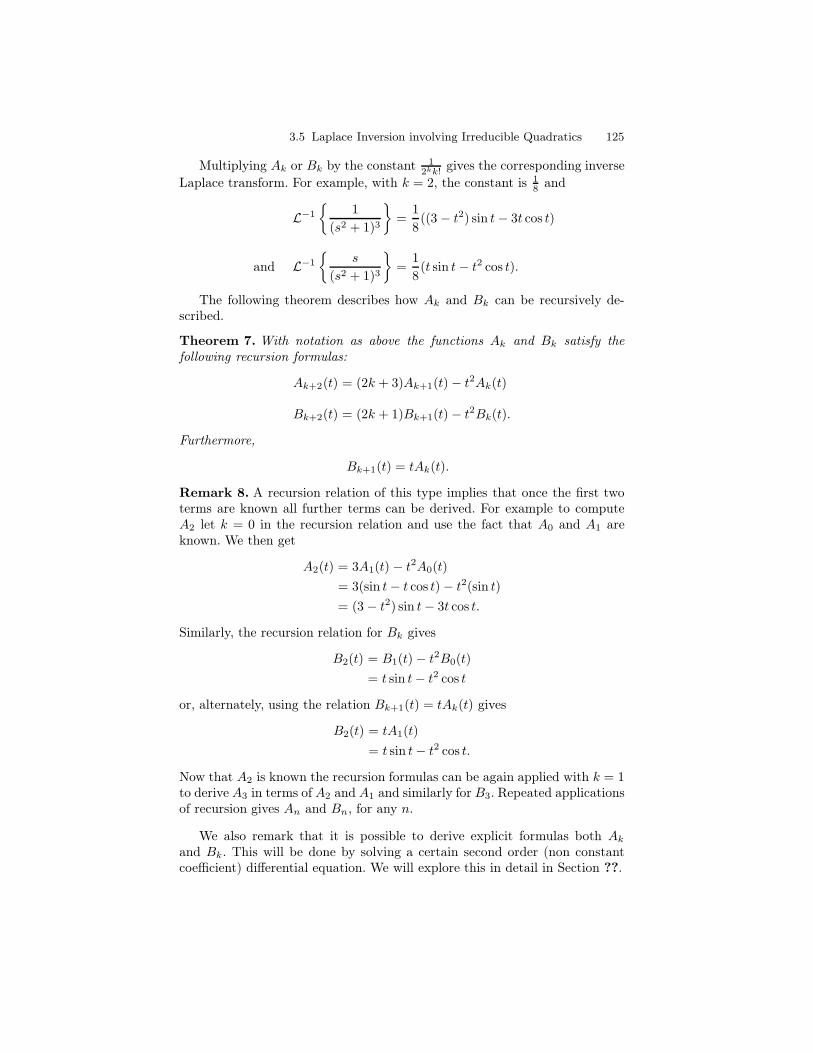
3.5 Laplace Inversion involving Irreducible Quadratics 125
Multiplying Ak or Bk by the constant 12kk!
gives the corresponding inverseLaplace transform. For example, with k = 2, the constant is 1
8 and
L−1
1
(s2 + 1)3
=1
8((3 − t2) sin t− 3t cos t)
and L−1
s
(s2 + 1)3
=1
8(t sin t− t2 cos t).
The following theorem describes how Ak and Bk can be recursively de-scribed.
Theorem 7. With notation as above the functions Ak and Bk satisfy thefollowing recursion formulas:
Ak+2(t) = (2k + 3)Ak+1(t)− t2Ak(t)
Bk+2(t) = (2k + 1)Bk+1(t)− t2Bk(t).
Furthermore,
Bk+1(t) = tAk(t).
Remark 8. A recursion relation of this type implies that once the first twoterms are known all further terms can be derived. For example to computeA2 let k = 0 in the recursion relation and use the fact that A0 and A1 areknown. We then get
A2(t) = 3A1(t) − t2A0(t)
= 3(sin t− t cos t)− t2(sin t)= (3 − t2) sin t− 3t cos t.
Similarly, the recursion relation for Bk gives
B2(t) = B1(t)− t2B0(t)
= t sin t− t2 cos t
or, alternately, using the relation Bk+1(t) = tAk(t) gives
B2(t) = tA1(t)
= t sin t− t2 cos t.
Now that A2 is known the recursion formulas can be again applied with k = 1to derive A3 in terms of A2 and A1 and similarly for B3. Repeated applicationsof recursion gives An and Bn, for any n.
We also remark that it is possible to derive explicit formulas both Ak
and Bk. This will be done by solving a certain second order (non constantcoefficient) differential equation. We will explore this in detail in Section ??.
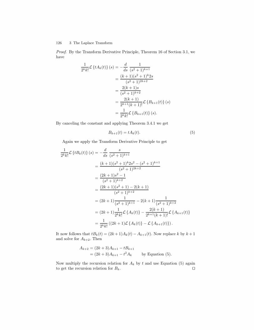
126 3 The Laplace Transform
Proof. By the Transform Derivative Principle, Theorem 16 of Section 3.1, wehave
1
2kk!LtAk(t) (s) = − d
ds
1
(s2 + 1)k+1
=(k + 1)(s2 + 1)k2s
(s2 + 1)2k+2
=2(k + 1)s
(s2 + 1)k+2
=2(k + 1)
2k+1(k + 1)!LBk+1(t) (s)
=1
2kk!LBk+1(t) (s).
By canceling the constant and applying Theorem 3.4.1 we get
Bk+1(t) = tAk(t). (5)
Again we apply the Transform Derivative Principle to get
1
2kk!LtBk(t) (s) = − d
ds
s
(s2 + 1)k+1
=(k + 1)(s2 + 1)k2s2 − (s2 + 1)k+1
(s2 + 1)2k+2
=(2k + 1)s2 − 1
(s2 + 1)k+2
=(2k + 1)(s2 + 1)− 2(k + 1)
(s2 + 1)k+2
= (2k + 1)1
(s2 + 1)k+1− 2(k + 1)
1
(s2 + 1)k+2
= (2k + 1)1
2kk!LAk(t) − 2(k + 1)
2k+1(k + 1)!LAk+1(t)
=1
2kk!((2k + 1)LAk(t) − LAk+1(t)) .
It now follows that tBk(t) = (2k+ 1)Ak(t)−Ak+1(t). Now replace k by k+ 1and solve for Ak+2. Then
Ak+2 = (2k + 3)Ak+1 − tBk+1
= (2k + 3)Ak+1 − t2Ak by Equation (5).
Now multiply the recursion relation for Ak by t and use Equation (5) againto get the recursion relation for Bk. ut
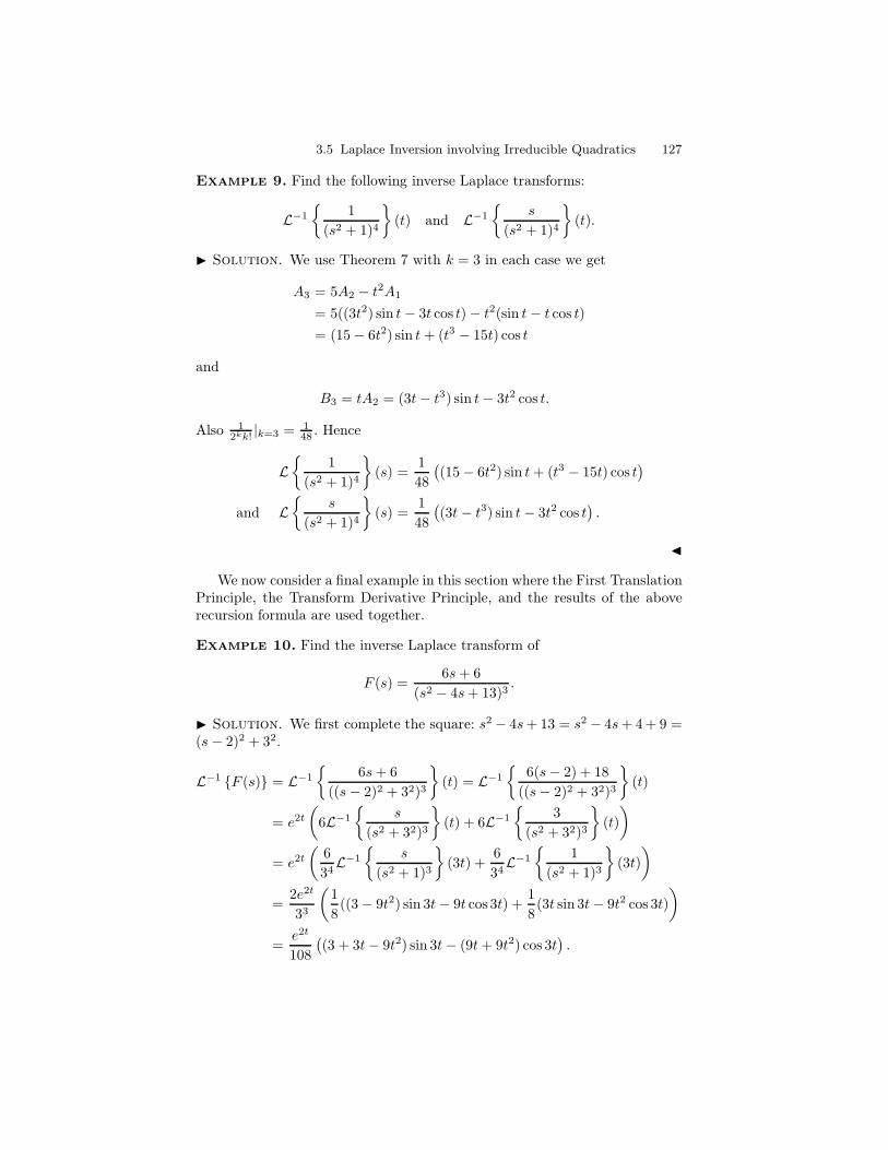
3.5 Laplace Inversion involving Irreducible Quadratics 127
Example 9. Find the following inverse Laplace transforms:
L−1
1
(s2 + 1)4
(t) and L−1
s
(s2 + 1)4
(t).
I Solution. We use Theorem 7 with k = 3 in each case we get
A3 = 5A2 − t2A1
= 5((3t2) sin t− 3t cos t)− t2(sin t− t cos t)
= (15− 6t2) sin t+ (t3 − 15t) cos t
and
B3 = tA2 = (3t− t3) sin t− 3t2 cos t.
Also 12kk! |k=3 = 1
48 . Hence
L
1
(s2 + 1)4
(s) =1
48
(
(15− 6t2) sin t+ (t3 − 15t) cos t)
and L
s
(s2 + 1)4
(s) =1
48
(
(3t− t3) sin t− 3t2 cos t)
.
J
We now consider a final example in this section where the First TranslationPrinciple, the Transform Derivative Principle, and the results of the aboverecursion formula are used together.
Example 10. Find the inverse Laplace transform of
F (s) =6s+ 6
(s2 − 4s+ 13)3.
I Solution. We first complete the square: s2 − 4s+ 13 = s2 − 4s+ 4 + 9 =(s− 2)2 + 32.
L−1 F (s) = L−1
6s+ 6
((s− 2)2 + 32)3
(t) = L−1
6(s− 2) + 18
((s− 2)2 + 32)3
(t)
= e2t
(
6L−1
s
(s2 + 32)3
(t) + 6L−1
3
(s2 + 32)3
(t)
)
= e2t
(
6
34L−1
s
(s2 + 1)3
(3t) +6
34L−1
1
(s2 + 1)3
(3t)
)
=2e2t
33
(
1
8((3− 9t2) sin 3t− 9t cos 3t) +
1
8(3t sin 3t− 9t2 cos 3t)
)
=e2t
108
(
(3 + 3t− 9t2) sin 3t− (9t+ 9t2) cos 3t)
.
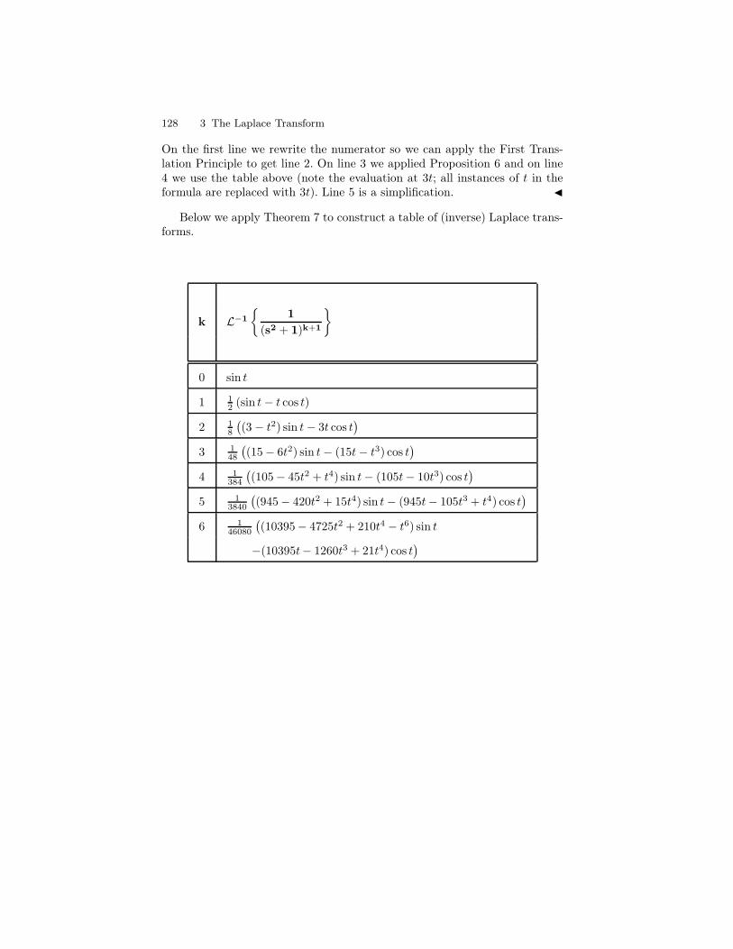
128 3 The Laplace Transform
On the first line we rewrite the numerator so we can apply the First Trans-lation Principle to get line 2. On line 3 we applied Proposition 6 and on line4 we use the table above (note the evaluation at 3t; all instances of t in theformula are replaced with 3t). Line 5 is a simplification. J
Below we apply Theorem 7 to construct a table of (inverse) Laplace trans-forms.
k L−1
1
(s2 + 1)k+1
0 sin t
1 12 (sin t− t cos t)
2 18
(
(3 − t2) sin t− 3t cos t)
3 148
(
(15− 6t2) sin t− (15t− t3) cos t)
4 1384
(
(105− 45t2 + t4) sin t− (105t− 10t3) cos t)
5 13840
(
(945− 420t2 + 15t4) sin t− (945t− 105t3 + t4) cos t)
6 146080
(
(10395− 4725t2 + 210t4 − t6) sin t
−(10395t− 1260t3 + 21t4) cos t)
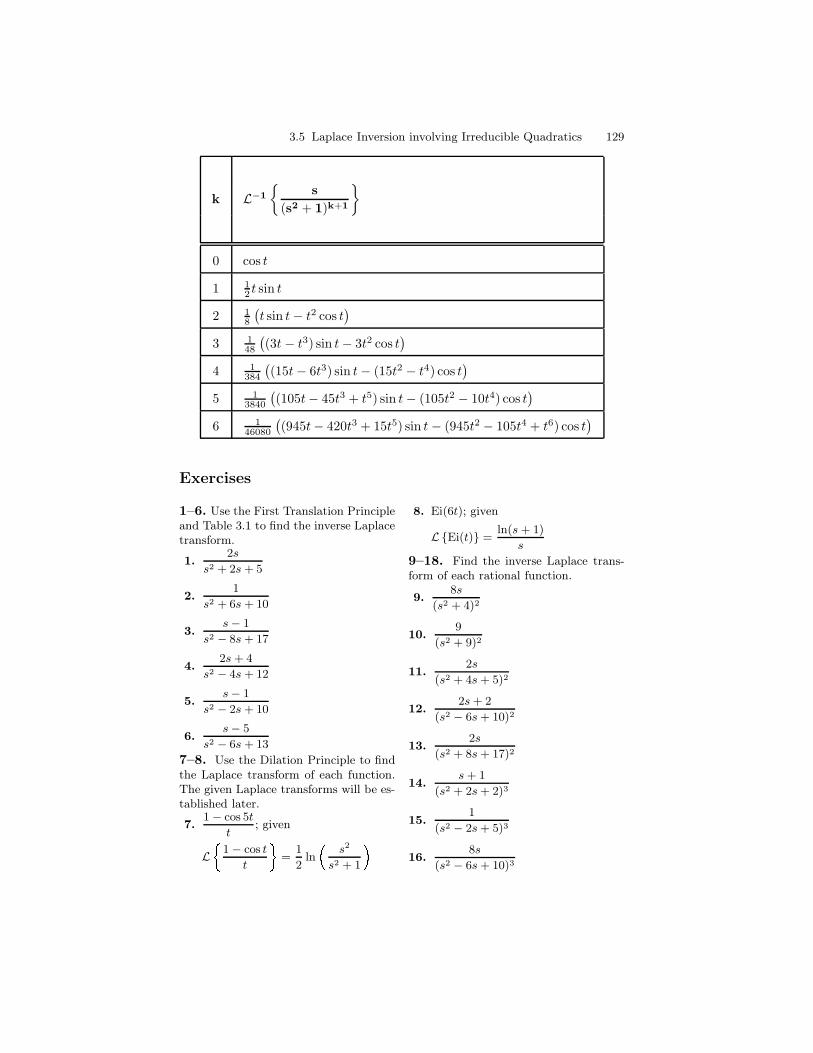
3.5 Laplace Inversion involving Irreducible Quadratics 129
k L−1
s
(s2 + 1)k+1
0 cos t
1 12 t sin t
2 18
(
t sin t− t2 cos t)
3 148
(
(3t− t3) sin t− 3t2 cos t)
4 1384
(
(15t− 6t3) sin t− (15t2 − t4) cos t)
5 13840
(
(105t− 45t3 + t5) sin t− (105t2 − 10t4) cos t)
6 146080
(
(945t− 420t3 + 15t5) sin t− (945t2 − 105t4 + t6) cos t)
Exercises
1–6. Use the First Translation Principleand Table 3.1 to find the inverse Laplacetransform.
1.2s
s2 + 2s + 5
2.1
s2 + 6s + 10
3.s − 1
s2 − 8s + 17
4.2s + 4
s2 − 4s + 12
5.s − 1
s2 − 2s + 10
6.s − 5
s2 − 6s + 13
7–8. Use the Dilation Principle to findthe Laplace transform of each function.The given Laplace transforms will be es-tablished later.
7.1 − cos 5t
t; given
L 1 − cos t
t =1
2ln s2
s2 + 1
8. Ei(6t); given
LEi(t) =ln(s + 1)
s
9–18. Find the inverse Laplace trans-form of each rational function.
9.8s
(s2 + 4)2
10.9
(s2 + 9)2
11.2s
(s2 + 4s + 5)2
12.2s + 2
(s2 − 6s + 10)2
13.2s
(s2 + 8s + 17)2
14.s + 1
(s2 + 2s + 2)3
15.1
(s2 − 2s + 5)3
16.8s
(s2 − 6s + 10)3
130 3 The Laplace Transform
17.s − 4
(s2 − 8s + 17)4
18.2
(s2 + 4s + 8)3
19–20. Use Theorem 7 to compute thefollowing inverse Laplace transforms.
19.1
(s2 + 1)5
20.s
(s2 + 1)5
3.6 The Laplace Transform Method
The Laplace transform is particularly well suited for solving certain types ofdifferential equations, namely the constant coefficient linear differentialequations
any(n) + an−1y
(n−1) + · · ·+ a1y′ + a0y = f(t), (1)
where a0, . . ., an are constants, the function f(t) is continuous, and the initialvalues of the unknown function y(t) are also specified:
y(0) = y0, y′(0) = y1, . . . , y
(n−1)(0) = yn−1.
Equation (1), with the initial values of y(t), is known as an initial valueproblem. In this chapter and the next we will assume f is an exponentialpolynomial. The basic theory of this type of differential equation will be dis-cussed in detail in Chapter 4. For now, we will only study how the Laplacetransform leads very quickly to a formula for y(t).
The Laplace transform method for solving Equation (1) is based on thelinearity property of the Laplace transform (Theorem 3.1.1) and the followingformula which expresses the Laplace transform of the derivative of a function.
Theorem 1. Suppose f(t) is an exponential polynomial and F (s) = Lf(t) .Then f ′(t) is an exponential polynomial and
Input Derivative Principle:
The First Derivative
Lf ′(t) = sF (s)− f(0)
Proof. By Exercise 3.4.36 if f is an exponential polynomial then so is f ′(t). Weapply integration by parts to the improper integral defining Lf ′(t), takinginto account the convention that g(t)|∞0 is a shorthand for limt→∞(g(t)−g(0)),provided the limit exists. Let u = e−st and dv = f ′(t) dt then
3.6 The Laplace Transform Method 131
Lf ′(t) (s) =
∫ ∞
0
e−stf ′(t) dt
=(
f(t)e−st)∣
∣
∞0−∫ ∞
0
(−s)e−stf(t) dt
= −f(0) +
∫ ∞
0
e−stf(t) dt
= sLf(t) (s)− f(0).
The transition from the second to the third line is a result of the fact thatexponential polynomials, f(t), satisfy limt→∞ f(t)e−st = 0, for s large. (SeeEquation 3.1.5.) ut
Example 2. Verify the validity of Theorem 1 for the following functions:
f(t) = 1, f(t) = eat, and f(t) = cos 3t.
I Solution.
• If f(t) = 1, then f ′(t) = 0 so Lf ′(t) = 0, and
sF (s)− f(0) = s1
s− 1 = 0 = Lf ′(t) .
• If f(t) = eat, then f ′(t) = aeat so Lf ′(t) =a
s− a and
sF (s)− f(0) =s
s− a − 1 =a
s− a = Lf ′(t) .
• If f(t) = cos 3t then f ′(t) = −3 sin3t so Lf ′(t) = − 9
s2 + 9and
sF (s)− f(0) = ss
s2 + 9− 1 = − 9
s2 + 9= Lf ′(t) .
J
Example 3. Solve the first order linear differential equation:
y′ − 3y = 1, y(0) = 1
I Solution. As is our convention, let Y (s) = Ly(t). We apply the Laplacetransform to both sides of the given equation and use linearity (Theorem 3.1.1)and the input derivative formula (Theorem 1) just verified to get
Ly′ − 3y = L1
L y′ − 3Ly =1
s
sY (s)− y(0)− 3Y (s) =1
s.
132 3 The Laplace Transform
We now have an algebraic equation for which we solve for Y (s). Since y(0) = 1we get
Y (s) =1
s− 3
(
1 +1
s
)
=1
s− 3+
1
s(s− 3).
A partial fraction decomposition gives
Y (s) =1
s− 3+
1
3
1
s− 3− 1
3
1
s=
4
3
1
s− 3− 1
3
1
s.
We recover y(t) from Y (s) by Laplace inversion. We obtain
y(t) =4
3L−1
1
s− 3
− 1
3L−1
1
s
=4
3e3t − 1
3.
J
Let’s consider another example.
Example 4. Solve the first order linear differential equation
y′ + y = sin t, y(0) = 0.
I Solution. Letting Y (s) = Ly(t), we equate the Laplace transform ofeach side of the equation to obtain
(s+ 1)Y (s) =1
s2 + 1.
Solving for Y (s) and decomposing Y (s) into partial fractions gives
Y (s) =1
2
(
1
s+ 1− s
s2 + 1+
1
s2 + 1
)
.
Inversion of the Laplace transform gives
y(t) = L−1 Y (s) =1
2
(
e−t − cos t+ sin t)
.
J
As we have already remarked if f(t) is an exponential polynomial so isf ′(t). Inductively, all orders of the derivative of f(t) are exponential polyno-mials. Thus we may apply Theorem 1 with f(t) replaced by f ′(t) (so that(f ′)′ = f ′′) to get
Lf ′′(t) = sLf ′(t) − f ′(0)
= s (sLf(t) − f(0))− f ′(0)
= s2Lf(t) − sf(0)− f ′(0).
Thus we have arrived at the following formula for expressing the Laplacetransform of f ′′(t) in terms of Lf(t) and the initial values f(0) and f ′(0).
3.6 The Laplace Transform Method 133
Corollary 5. Suppose f(t) is an exponential polynomial. Then
Input Derivative Principle:
The Second Derivative
Lf ′′(t) = s2F (s)− sf(0)− f ′(0).
The process used to determine Corollary 5 for the Laplace transform of asecond derivative can be repeated to arrive at a formula for the Laplace trans-form of the nth derivative of an exponential polynomial, which we summarizein the following theorem.
Theorem 6. Suppose f(t) is an exponential polynomial and Lf(t) = F (s).Suppose n ≥ 1. Then
Input Derivative Principle:
The nth Derivative
L
f (n)(t)
= snF (s)− sn−1f(0)− sn−2f ′(0)− · · · − f (n−1)(0).
For n = 3 and n = 4, this formula becomes
Lf ′′′(t) = s3F (s)− s2f(0)− sf ′(0)− f ′′(0)
and L
f (4)(t)
= s4F (s)− s3f(0)− s2f ′(0)− sf ′′(0)− f ′′′(0).
If f(0) = f ′(0) = · · · = f (n−1) = 0 then Theorem 6 has the particularlysimple form
Lf ′(t) = snF (s).
In words, the operation of differentiating n-times on the space of elementaryfunctions with derivatives (up to order n − 1) vanishing at 0, corresponds,under the Laplace transform, to the algebraic operation of multiplying by sn
on the space Rpr(s) of proper rational functions.Let’s consider some examples of how Theorem 6 is used to solve some
types of differential equations.
Example 7. Solve the initial value problem
y′′ − y = 0, y(0) = 0, y′(0) = 1.
134 3 The Laplace Transform
I Solution. As usual, let Y (s) = Ly(t) and apply the Laplace transformto both sides of the differential equation to obtain
s2Y (s)− 1− Y (s) = 0.
Now solve for Y (s) and decompose in partial fractions to get
Y (s) =1
s2 − 1=
1
2
1
s− 1− 1
2
1
s+ 1.
Then applying the inverse Laplace transform to Y (s) gives
y(t) = L−1 Y (s) =1
2(et − e−t).
J
Example 8. Solve the initial value problem
y′′ + 4y′ + 4y = 2te−2t, y(0) = 1, y′(0) = −3.
I Solution. Let Y (s) = Ly(t) where, as usual, y(t) is the unknown solu-tion. Applying the Laplace transform gives the algebraic equation
s2Y (s)− s+ 3 + 4(sY (s)− 1) + 4Y (s) =2
(s+ 2)2,
which can be solved for Y (s) to give
Y (s) =s+ 1
(s+ 2)2+
2
(s+ 2)4.
The partial fraction decomposition gives
Y (s) =1
s+ 2− 1
(s+ 2)2+
2
(s+ 2)4.
Taking the inverse Laplace transform y(t) = L−1 Y (s) then gives
y(t) = e−2t − te−2t +1
3t2e−2t.
J
It is worth pointing out in this last example that in solving for Y (s) we kept
the part of Y (s) that came from the initial values, namelys+ 1
(s+ 2)2, distinct
from that determined by the right-hand side of the equation, namely2
(s+ 2)4.
By not combining these into a single proper rational function before computingthe partial fraction decomposition, we have simplified the computation of thepartial fractions. This is a typical situation and one that you should be awareof when working on exercises.
3.6 The Laplace Transform Method 135
Example 9. Solve the initial value problem
y′′ + β2y = cosωt, y(0) = y′(0) = 0,
where we assume that β 6= 0 and ω 6= 0.
I Solution. Let Y (s) = Ly(t) and apply the Laplace transform to theequation. We then solve algebraically for Y (s) to get
Y (s) =s
(s2 + β2)(s2 + ω2).
We will break our analysis into two cases: (1) β2 6= ω2 and (2) β2 = ω2.
Case 1: β2 6= ω2.In this case we leave it as an exercise to verify that the partial fraction
decomposition of Y (s) is
Y (s) =1
ω2 − β2
(
s
s2 + β2− s
s2 + ω2
)
,
so that the solution y(t) = L−1 Y (s) is
y(t) =cosβt− cosωt
ω2 − β2.
Case 2: β2 = ω2.In this case
Y (s) =s
(s2 + ω2)2.
Applying the Dilation Principle and Theorem 3.5.7 gives
y(t) =1
2ωt sinωt.
J
Example 10. Solve the initial value problem
y′′′ − y′′ + y′ − y = 10e2t, y(0) = y′(0) = y′′(0) = 0.
I Solution. Let Y (s) = Ly(t) where y(t) is the unknown solution. Weapply the Laplace transform L to get
s3Y (s)− s2Y (s) + sY (s)− Y (s) =10
s− 2.
Solving for Y (s) and applying the partial fraction decomposition gives
136 3 The Laplace Transform
Y (s) =10
(s3 − s2 + s− 1)(s− 2)
=10
(s− 1)(s2 + 1)(s− 2)
=−5
s− 1+
2
s− 2+
1 + 3s
s2 + 1.
Now apply the inverse Laplace transform to get
y(t) = −5et + 2e2t + sin t+ 3 cos t.
J
We conclude this section by looking at what the Laplace transform tells usabout the solution of the second order linear constant coefficient differentialequation
ay′′ + by′ + cy = f(t), y(0) = y0, y′(0) = y1, (2)
where f(t) is an exponential polynomial, and a, b, and c are real constants.Applying the Laplace transform to Equation (2) (where Y (s) is the Laplacetransform of the unknown function y(t), as usual) gives
a(s2Y (s)− sy0 − y1) + b(sY (s)− y0) + cY (s) = F (s).
If we let P (s) = as2+bs+c (P (s) is known as the characteristic polynomialof the differential equation), then the above equation can be solved for Y (s)in the form
Y (s) =(as+ b)y0 + ay1
P (s)+F (s)
P (s)= Y1(s) + Y2(s). (3)
Notice that Y1(s) depends only on P (s), which is determined by the left-hand side of the differential equation, and the initial values y0 and y1, whileY2(s) depends only on P (s) and the function f(t) on the right-hand side ofthe equation. The function f(t) is usually called the input function for thedifferential equation. Taking inverse Laplace transforms we can write
y(t) = L−1 Y (s) = L−1 Y1(s) + L−1 Y2(s) = y1(t) + y2(t).
The function y1(t) is the solution of Equation (2) obtained by taking f(t) = 0,while y2(t) is the solution obtained by specifying that the initial conditions bezero, i.e., y0 = y1 = 0. Thus, y1(t) is referred to as the zero-input solution,while y2(t) is referred to as the zero-state solution. The terminology comesfrom engineering applications. You will be asked to compute further examplesin the exercises, and addtional consequences of Equation (3) will be developedin Chapter 5.
Exercises
3.6 The Laplace Transform Method 137
1–31. For the following differentialequations use the Laplace transformmethod. Determine both Y (s) and thesolution y(t).
1. y′ − 4y = 0, y(0) = 2
2. y′ − 4y = 3, y(0) = 2
3. y′ − 4y = 16t, y(0) = 2
4. y′ − 4y = e4t, y(0) = 0
5. y′ + 2y = 3et, y(0) = 2
6. y′ + 2y = te−2t, y(0) = 0
7. y′ + 9y = 81t2, y(0) = 1
8. y′ − 3y = cos t, y(0) = 0
9. y′ − 3y = 50 sin t, y(0) = 1
10. y′ + y = 2t sin t, y(0) = 1
11. y′ − 3y = 2e3t cos t, y(0) = 1
12. y′ − y = 10e2t sin 3t, y(0) = −2
13. y′′ + 3y′ + 2y = e2t,y(0) = 1, y′(0) = 1
14. y′′ − 4y′ − 5y = 25t,y(0) = −1 y′(0) = 0
15. y′′ + 4y = 8,y(0) = 2, y′(0) = 1
16. y′′ + 4y′ + 4y = e−2t,y(0) = 0 y′(0) = 1
17. y′′ + 4y′ + 4y = 4 cos 2t,y(0) = 0 y′(0) = 1
18. y′′ − 3y′ + 2y = 4,y(0) = 2, y′(0) = 3
19. y′′ − 3y′ + 2y = et,y(0) = −3, y′(0) = 0
20. y′′ + 2y′ − 3y = 13 sin 2t,y(0) = 0, y′(0) = 0
21. y′′ + 6y′ + 9y = 50 sin t,y(0) = 0, y′(0) = 2
22. y′′ + 25y = 0,y(0) = 1, y′(0) = −1
23. y′′ + 8y′ + 16y = 0,y(0) = 1
2, y′(0) = 2
24. y′′ − 4y′ + 4y = 4e2t, y(0) =−1, y′(0) = −4
25. y′′ + y′ + y = 0,y(0) = 1, y′(0) = 0
26. y′′ + 4y′ + 4y = 16t sin 2t,y(0) = 1 y′(0) = 0
27. y′′ + 4y = sin 3t,y(0) = 0 y′(0) = 1.
28. y′′′ − y′′ = t,y(0) = 0, y′(0) = 1, y′′(0) = 0
29. y′′′ − y′′ + y′ − y = t,y(0) = 0, y′(0) = 0, y′′(0) = 0
30. y′′′ − y′ = 6 − 3t2,y(0) = 1, y′(0) = 1, y′′(0) = 1
31. y(4) − y = 0, y(0) = 1, y′(0) =0, y′′(0) = 0, y′′′(0) = 0
32–35. For each of the following differ-ential equations, find the zero-state solu-tion. Recall that the zero-state solutionis the solution with all initial conditionsequal to zero.
32. y′′ + 4y′ + 13y = 0
33. y′′ + 4y′ + 3y = 6
34. y′′ − y = cos 3t
35. y′′ + y = 4t sin t
138 3 The Laplace Transform
3.7 Laplace Transform Correspondences
Suppose q(s) be a real (complex) polynomial. Let Rq (Rq,C) be the set of allproper real (complex) rational functions with q in the denominator. Let Eq(Eq,C) be the set of all real (complex) exponential polynomials whose Laplacetransform is in Rq (Rq,C). Symbolically, we would write
Rq =
p(s)
q(s): deg(p(s)) < deg(q(s))
and Eq = f ∈ E : Lf(s) ∈ Rq ,
where the polynomials p(s) are real. A similar description can be given forRq,C
and Eq,C. Keep in mind that q(s) is a fixed polynomial. In this section we areinterested in obtaining an explicit description of Eq and Eq,C. Consider a simpleexample. Let q(s) = s2 − 1 = (s − 1)(s + 1). How can we explicitly describeEq? Observe that any proper rational function with q(s) in the denominator
is of the form p(s)(s−1)(s+1) , where p(s) is a polynomial of degree one. A partial
fraction decomposition will have the form
p(s)
q(s)=
A1
s− 1+
A2
s+ 1,
where A1 and A2 are in R, and its inverse Laplace transform is
A1et +A2e
−t.
Thus Eq is the set of all real linear combinations of et, e−t. (It is the sameargument to show that Eq,C is the set of all complex linear combinations ofet, e−t.) Notice how efficient this description is: all we needed to find werethe two functions, et and e−t, and all other functions in Eq are given by takinglinear combinations. This is a much more explicit description than just sayingthat Eq is the set of functions that have Laplace transform with q(s) = s2−1 inthe denominator. This idea we want to generalize for any polynomial q. It willintroduce important notions about linear spaces, namely, spanning sets, linearindependence, and bases. The following theorem establishes a fundamentalproperty for the sets Eq, Eq,C, Rq, and Rq,C.
Theorem 1. Let q(s) be a real (complex) polynomial. Then Eq (Eq,C) and Rq
(Rq,C) are real (complex) linear spaces.
Proof. We will prove the real case; the complex case is handled in the sameway. Let’s begin with Rq. Suppose p1(s)
q(s) and p2(s)q(s) are in Rq. Then
p1(s)
q(s)+p2(s)
q(s)=p1(s) + p2(s)
q(s)∈ Rq.
If c ∈ R and p(s)q(s) ∈ Rq then
3.7 Laplace Transform Correspondences 139
c · p(s)q(s)
=cp(s)
q(s)∈ Rq.
These two calculations show that Rq is closed under addition and scalar mul-tiplication. This means Rq is a linear space.
Now suppose f1(t) and f2(t) are in Eq. Since their Laplace transforms areboth in Rq so is their sum and since the Laplace transform is linear we have
Lf1(t) + f2(t) = Lf1(t)+ Lf2(t) ∈ Rq.
This means f1(t) + f2(t) is in Eq. Let c ∈ R and f(t) ∈ Eq. Then
Lcf(t) = cLf(t) ∈ Rq
and again this means that cf(t) ∈ Eq. Thus Eq is a linear space. ut
Knowing that Eq is a linear space implies that it is closed under the op-eration of taking linear combinations. But more is true. We will show thatthere are finitely many functions f1, . . . , fn ∈ Eq so that Eq is precisely the setof all their linear combinations. Further, we will give an algorithm for find-ing a canonical set of such functions based entirely on the roots of q(s) andtheir multiplicities. Keep the simple example we did above in mind. Whenq(s) = s2 − 1 we showed that Eq is the set of all linear combinations of twofunctions, et and e−t.
To be able to speak precisely about these notions we begin by introducingthe concept of spanning sets.
Spanning Sets
Suppose F is a real or complex linear space of functions defined on a commoninterval I. Suppose f1, . . . , fn are in F . The set of all linear combinations
c1f1 + · · ·+ cnfn,
is called the span of f1, . . . fn and denoted by Span f1, . . . , fn. If F is areal linear space then the scalars c1, . . . , cn are understood to be real numbers.Similarly, if F is a complex linear space then the scalars c1, . . . , cn are thecomplex numbers. If it is unclear which scalars are in use we will use thenotation SpanR f1, . . . , fn or SpanC f1, . . . , fn to distinguish the cases. IfF = Span f1, . . . , fn we will refer to the set f1, . . . , fn as a spanningset for F . In the example above where q(s) = s2 − 1 we can say that Eq isthe span of et, e−t or that et, e−t is a spanning set for Eq. However, thenotation Eq = Span et, e−t is much simpler.
Theorem 2. Let F = Span f1, . . . , fn be as above. Then E is a linear space.
140 3 The Laplace Transform
Proof. It should be intuitively clear that F is closed under addition and scalarmultiplication: when we add two linear combinations or multiply a linearcombination by a scalar we get another such linear combination. However, tobe pedantic, here are the details. Suppose a1f1+· · ·+anfn and b1f1+· · ·+bnfn
are in F . Then
a1f1 + · · ·+ anfn + b1f1 + · · ·+ bnfn = (a1 + b1)f1 + · · · (an + bn)fn ∈ F .
Thus F is closed under addition. If c is a scalar then
c · (a1f1 + · · ·+ anfn) = ca1fn + · · · canfn ∈ F .
Thus F is closed under scalar multiplication. It follows that F is a linear space(real or complex depending on the scalars used). ut
We should note that a linear space can be spanned by more than onespanning set. The following example explains what we mean.
Example 3. Let q(s) + s2 − 1. Show that
S1 =
et, e−t
, S2 = sinh t, cosh t , and S3 =
et, e−t, et + e−t
are spanning sets for Eq.
I Solution. We need to show that each set given above is a spanning set forEq. We have already established that Eq = SpanR S1 . Recall that cosh t =et+e−t
2 and sinh t = et−e−t
2 . Each are linear combinations of et, e−t andhence in Eq. Since Eq is a linear space it is closed under linear combinations.It follows that SpanR S2 ⊂ Eq. Now observe that et = cosh t+sinh t
2 ande−t = cosh t−sinh t
2 . Reasoning as above, both et and e−t are linear combinationsof cosh t and sinh t. Hence Eq = SpanR S1 ⊂ SpanR S2. It follows nowthat Eq = SpanR S2 . Since each function in S3 is a linear combinationof functions in S1 it follows that SpanR S3 ⊂ SpanR S1 = Eq. On theother hand, S1 ⊂ S3 and thus SpanR S1 ⊂ SpanR S3. It follows now thatEq = SpanR S1 = SpanR S2 = SpanR S3 . J
You will notice that in the example above S3 contains 3 functions, et,e−t and et + e−t. There is a certain redundancy in using all three functionsin a spanning set when only two are necessary. Specifically, observe that thethird function depends linearly on the first two (it is their sum) so that alinear combination of all three functions in S3 can be rewritten as a linearcombination in terms of only the first two functions:
c1et + c2e
−t + c3(et + e−t) = (c1 + c3)e
t + (c1 + c3)e−t.
We root out such dependencies in spanning sets by the concept of linearindependence.
3.7 Laplace Transform Correspondences 141
Linear Independence
A set of functions f1, . . . , fn, defined on some interval I, is said to be lin-early independent if the equation
a1f1 + · · ·+ anfn = 0 (1)
implies that all the coefficients a1, . . . , an are zero. Otherwise, we say f1, . . . , fnis linearly dependent.2
One must be careful about this definition. We do not try to solve Equation(1) for the variable t. Rather, we are given that this equation is valid forall t ∈ I. With this information the focus is on what this says about thecoefficients a1, . . . , an; are they necessarily zero or not.
Again, we must say something about the scalars in use. We use the term’linearly independent over R’ or the term ‘linearly independent over C’ if thescalars in use are real or complex, respectively. However, in most cases thecontext will determine which is meant.
Let’s consider an example of a set that is not linearly independent.
Example 4. Show that the set et, e−t, et + e−t is linearly dependent.
I Solution. This is the set S3 that we considered above. To show that a setis linearly dependent we need only show that we can find a linear combinationthat adds up to 0 with coefficients not all zero. One such is
(1)et + (1)e−t + (−1)(et + e−t) = 0.
The coefficients, highlighted by the parentheses, are 1, 1, and −1 and are notall zero. Thus S3 is linearly dependent. As noted above the dependency isclearly seen in that the third function is the sum of the first two. J
Now let’s return to the basic example that began this section.
Example 5. Show that the set et, e−t is linearly independent.
I Solution. In this case we need to show that the only way a linear combi-nation adds up to zero is for the coefficients to be zero. Thus we consider theequation
a1et + a2e
−t = 0, (2)
for all t ∈ R. In order to conclude linear independence we need to show thata1 and a2 are zero. There are many ways this can be done. Below we showthree approaches. Of course, only one is necessary.
Method 1: Evaluation at specified points Let’s evaluate Equation (2)at two points: t = 0 and t = ln 2.
2A grammatical note: We say f1, . . . , fn are linearly independent if the set
f1, . . . , fn is linearly independent.
142 3 The Laplace Transform
t = 0 a1 + a2 = 0
t = ln 2 a1(2) + a2(1/2) = 0.
These two equations have only one simultaneous solution, namely, a1 = 0 anda2 = 0. Thus et, e−t is linearly independent.
Method 2: Differentiation Take the derivative of Equation (2) to geta1e
t − a2e−t = 0. Evaluating Equation (2) and the derivative at t = 0 gives
a1 + a2 = 0
a2 − a2 = 0.
The only solution to these equations is a1 = 0 and a2 = 0. Hence et, e−t islinearly independent.
Method 3: The Laplace Transform Here we take the Laplace transformof Equation (2) to get
a1
s− 1+
a2
s+ 1= 0,
which is an equation valid for all s > 1, and consider the right-hand limit as sapproaches 1. If a1 is not zero then a1
s−1 has an infinite limit while the secondterm a2
s+1 has a finite limit. But this cannot be as the sum is 0. It must bethat a1 = 0 and therefore a2e
−t = 0. This equation in turn implies a2 = 0.Now it follows that et, e−t is linearly independent. J
We will see Method 3 used in a more general context later in this section.In the comment following the solution to Example 3 we noted that therewas some redundancy in the linearly dependent set S3; it contained an extrafunction that was not needed to span Eq, for q(s) = s2 − 1. This is generallytrue of dependent sets; if fact, it characterizes them.
Theorem 6. A set of functions f1, . . . , fn in a linear space F is linearlydependent if and only if one of the functions is a linear combination of theothers.
Proof. Let’s assume that one of the functions, f1 say, is a linear combinationsof the others. Then we can write f1 = a2f2 + · · ·+ anfn, which is equivalentto
f1 − a2f2 − a3f3 − · · · − anfn = 0.
Since not all of the coefficients are zero (the coefficient of f1 is 1) it follows thatf1, . . . , fn is linearly dependent. On the other hand, suppose f1, . . . , fnis linearly dependent. Then there are scalars, not all zero, such that a1f1 +· · ·+ anfn = 0. By reordering if necessary, we may assume that a1 6= 0. Nowwe can solve for f1 to get
f1 = −a2
a1f2 − · · · −
−an
a1fn,
Thus one of the functions is a linear combination of the others. ut
3.7 Laplace Transform Correspondences 143
When we combine the notion of a spanning set and linear independencewe get what is called a basis.
Bases
A set of functions f1, . . . , fn is said to be a basis3 of a linear space F iff1, . . . , fn is linearly independent and a spanning set for F . Thus et, e−tis a basis of Eq, for q(s) = s2 − 1, because Eq = Span et, e−t and is linearlyindependent by Example 5. Whereas et, e−t, et + e−t is not a basis of Eqbecause, although it spans Eq it is not linearly independent.
The following theorem explains generally how a basis efficiently describesthe linear space it spans.
Theorem 7. Suppose B = f1, . . . , fn is a basis of a linear space F . If f ∈ Fthen there are unique scalars a1, . . . , an such that f = a1f1 + · · ·+ anfn.
Proof. The focus here is on the uniqueness of the scalars. Suppose f ∈ F .Since B is a basis it spans F . Thus we can express f as a linear combinationof f1, . . . , fn. Suppose now we can do this in two ways:
f = a1f1 + · · ·+ anfn
and f = b1f1 + · · ·+ bnfn.
By subtracting these two equations we get (a1 − b1)f1 + · · · (an − bn)fn = 0.Since B is linearly independent the coefficients ai−bi, i = 1, . . . , n are all zero.This means then that ai = bi, i = 1, . . . , n. Thus the scalars used to representf are unique. ut
From Examples 5 and 3 we see that for q(s) = s2 − 1 the sets
B1 =
et, e−t
and B2 = cosh t, sinh t
are both bases of Eq. Thus a linear space can have more than one basis.However, Theorem 7 states that once a basis of F is fixed each function in Fcan be written uniquely as a linear combination of functions in the basis.
We now reiterate our goal for this section in terms of the concepts we haveintroduced. For q(s) a fixed polynomial we will provide a standard methodto find a basis, Bq (Bq,C), for Eq (Eq,C). We will begin with the complex casefirst.
The Complex Linear Space Eq,C
Let q be a fixed (complex) polynomial. Let f ∈ Eq,C and F (s) = Lf(t).Then F (s) = p(s)
q(s) for some polynomial p(s). Suppose γ1, . . . , γl are the distinct
3A grammatical note: basis is the singular form of bases
144 3 The Laplace Transform
roots of q with multiplicities m1, . . . ,ml, respectively. Then q factors as q(s) =C(s − γ1)
m1 · · · (s − γl)ml . The partial fraction decomposition of a rational
function pq will involve terms of the form
1
(s− γi)k, 1 ≤ k ≤ mi.
We define the finite set Bq,C by
Bq,C =
tk−1eγit : k = 1, . . . ,mi and i = 1, . . . , l
. (3)
Since L
tk−1eγit
(k−1)!
= 1(s−γi)k , it follows that f(t) is a linear combination of
Bq,C and hence Eq,C ⊂ Span Bq,C. Note that we have dropped the factorialterms as these may be absorbed in the scalars of any linear combination.Since each simple exponential polynomial in Bq,C is in Eq,C we must haveSpan Bq,C ⊂ Eq,C. It now follows that Span Bq,C = Eq,C.
Example 8. If q(s) = (s2 + 9)2(s− 2) find Bq,C.
I Solution. The roots of q(s) are 3i with multiplicity 2, −3i with multi-plicity 2, and 2 with multiplicity 1. From Equation (3) we have
Bq,C =
e3it, e−3it, te3it, te−3it, et
.
J
We need to show that Bq,C is a linearly independent set. To do so weintroduce an useful lemma.
Lemma 9. Suppose f1(t), . . . , fl(t) are polynomials and λ1, . . . , λl are distinctcomplex numbers. Suppose
f1(t)eλ1t + · · ·+ fl(t)e
λlt = 0. (4)
Then fi = 0, for each i = 1, . . . l.
Proof. First let’s derive a useful formula. Let f(t) = amtm + · · ·+ a1t+ a0 be
a polynomial of degree m and λ a complex number. Then by Example 11 ofSection 3.1 we have L
tkeλt
= k!(s−λ)k+1 and hence
L
f(t)eλt
=
m∑
k=0
akk!
(s− λ)k+1=
f(s− λ)(s− λ)m+1
,
where f(s − λ) = a0(0!)(s − λ)m + a1(1!)(s − λ)m−1 + · · · + am(m!) is apolynomial of degreem obtained by adding the terms in the sum with commondenominator (s − λ)m+1. We observe that f is a polynomial of degree m.Further, if f(s−λ) = 0 then all the coefficients a0, . . . , am are zero and hencef = 0. With this in mind we proceed with the proof of the lemma as stated.
3.7 Laplace Transform Correspondences 145
Let us reorder the λi, if necessary, in such a way that λ1 is among thoseroots with the largest real part. Suppose fi has degree mi, i = 1, . . . , l. Wetake the Laplace transform of Equation (4) to get
f1(s− λ1)
(s− λ1)m1+1+ · · · fl(s− λl)
(s− λl)ml+1= 0, (5)
with notation as in the preceding paragraph. Equation 5 is valid for all complexnumbers s whose real part is larger than the real part of λ1. Now consider theright hand limit lims→λ+
1applied to Equation (5). Suppose f1(s − λ1) 6= 0.
Since λ1, . . . , λl are distinct, all terms have finite limits except for the first,which has an infinite limit. However, the sum of the limits must be zero, whichis impossible. We conclude that f1(s − λ1) = 0 and hence by the remarks inthe previous paragraph f1(s) = 0. We can now eliminate the first term fromEquation (5). Reorder the remaining λi’s if necessary so that λ2 is amongthe roots with the largest real part. By repeating the above argument we canconclude f2(s) = 0. Inductively, we conclude that fi(s) = 0, i = 1, . . .m. ut
We thus have the following theorem.
Theorem 10. Suppose q is a polynomial of degree n and λ1, . . . , λl the distinctroots with multiplicities m1, . . . ,ml, respectively. Then the set
Bq,C =
tk−1eλit : k = 1, . . . ,mi and i = 1, . . . , l
forms a basis of Eq,C.
Proof. We have already shown that Eq,C = Span Bq,C. To show linear inde-pendence suppose
∑
ai,ktk−1eλit = 0.
By first summing over k we can rewrite this as
f1(t)eλ1t + · · ·+ fl(t)e
λlt = 0,
where fi(t) =∑ml
k=1 ai,ktk−1, for each i = 1, . . . , l. By Lemma 9, fi = 0, for
i = 1, . . . , l, and hence all the coefficients ai,j are zero. This implies thatBq,C is linearly independent and hence a basis of Eq,C. ut
The finite set Bq,C is called the standard basis of Eq,C. Once the roots ofq and their multiplicities are determined it is straightforward to write downthe standard basis. Notice also that the number of terms in the standard basisfor Eq,C is the same as the degree of q.
Example 11. Find the standard basis Bq,C of Eq,C for each of the followingpolynomials:
146 3 The Laplace Transform
1. q(s) = s3 − s2. q(s) = s2 + 1
3. q(s) = (s− 2)4
4. q(s) = s2 + 4s+ 5
I Solution.
1. q(s) = s3 − s = s(s− 1)(s+ 1). The roots are 0, 1, and −1 and each rootoccurs with multiplicity 1. The standard basis of Eq,C is Bq,C = 1, e−t, et.
2. q(s) = s2 +1 = (s+ i)(s− i) The roots are i and −i each with multiplicity1. The standard basis of Eq,C is Bq,C =
eit, e−it
.
3. q(s) = (s− 2)4. Here the root is 2 with multiplicity 4. Thus the standardbasis of Eq,C is Bq,C =
e2t, te2t, t2e2t, t3e2t
.
4. q(s) = s2 + 4s+ 5 = (s+ 2)2 + 1 = (s− (−2 + i))(s− (−2− i)). Thus thestandard basis of Eq,C is Bq,C =
e(−2+i)t, e(−2−i)t
. J
The Real Linear Space Eq
Suppose q(s) is a real polynomial. We want to describe a real basis Bq of Eq.View q(s) as a complex polynomial. Recall that if λ = a+ ib is a complex rootwith multiplicity m then its conjugate λ = a− ib is also a root with the samemultiplicity. Thus non real roots of q(s) come in pairs
λ, λ
. By switchingthe order of the pair
λ, λ
and relabeling, if necessary, we can assume b > 0.In the standard basis Bq,C for Eq,C the functions
tkeλt, tkeλt
likewise come in pairs. Let Bq be the set obtained from Bq,C by replacing eachsuch pair with the real functions
tkeat cos bt, tkeat sin bt
,
(λ = a+ ib and b > 0). We will show below that the set Bq obtained in thisway is a basis of Eq; we call it the standard basis of Eq.
Consider the following example.
Example 12. Find Bq if q(s) = (s2 + 4)2(s− 6)3.
I Solution. The roots of q are ±2i with multiplicity 2 and 6 with multi-plicity 3. Thus
Bq,C =
e2it, e−2it, te2it, te−2it, e6t, te6t, t2e6t
.
The only conjugate pair of non real roots is 2i,−2i. It gives rise to pairsof functions
e2it, e−2it
and
te2it, te−2it
in Bq,C which are replaced bycos 2t, sin 2t and t cos 2t, t sin 2t, respectively. We thus obtain
Bq =
cos 2t, sin 2t, t cos 2t, t sin 2t, e6t, te6t, t2e6t
.
J
3.7 Laplace Transform Correspondences 147
Let’s now show that Bq is basis of Eq, for a real polynomial q(s). Sincewe can regard q(s) as a complex polynomial we have Rq ⊂ Rq,C and henceEq ⊂ Eq,C. By Theorem 7 of Section 3.1, Eq is precisely the set of all realvalued functions in Eq,C. We begin by showing Eq = SpanR Bq. Let λ be aroot of q(s). Either λ is real or is part of a non real root pair (λ, λ). If λ = ais a real root of q(s) with multiplicity m the function tkeat, k = 0, . . . ,m− 1,is in Bq and Bq,C, hence in Eq,C. Consider a non real root pair (λ, λ) of q(s),where λ = a+ ib with multiplicity m and b > 0. Let k be an integer between0 and m− 1. By Euler’s equation the associated pairs of functions are relatedby the following equations:
tkeλt = tkeat(cos bt+ i sin bt)
tkeλt = tkeat(cos bt− i sin bt)and
tkeat cos bt = 12
(
tkeλt + tkeλt)
tkeat sin bt = 12i
(
tkeλt − tkeλt) (6)
Notice that tkeat cos bt and tkeat sin bt are linear combinations of tkeλt andtkeλt and hence in Eq,C. If follows now that Bq ⊂ Eq,C and hence any functionin the real span of Bq is a real function in Eq,C and hence in Eq. This impliesSpanR Bq ⊂ Eq.
Now suppose f ∈ Eq. Then it is also in Eq,C and we can write f as a(complex) linear combination of functions in Bq,C. Briefly, we can write f =∑
µtkeλt, where the λ’s are among the roots of q(s), k is a nonnegative integerup to the multiplicity of λ less one, and µ is complex number for each pair(k, λ). Consider the two cases. Suppose λ is real. Let µ = α + iβ. ThenRe(µtkeλt) = αtkeλt is a real scalar multiple of a function in Bq. Supposeλ = a+ ib is non real, with b > 0. Then
Re(µtkeλt) = Re((α+ iβ)tkeat(cos bt+ i sin bt))
= αtkeat cos bt− βtkeat sin bt,
a real linear combination of functions in Bq. Since f is real these preced-ing calculations show that f(t) = Re(f(t)) =
∑
Re(µtkeλt) is a real lin-ear combination of functions in Bq. Thus f(t) ∈ SpanR Bq. It follows thatEq ⊂ SpanR Bq and hence Eq = SpanR Bq.
We proceed now to show that Bq is linearly independent. First consider apreliminary calculation. Let c1 and c2 be real numbers and λ = a + ib, withb > 0. Then by Equation (6) we have
c1tkeat cos bt+ c2t
keat sin bt =c1 − ic2
2tkeλt +
c1 + ic22
tkeλt.
If c1−ic2
2 = 0 or c1+ic2
2 = 0 then c1 = c2 = 0. Now suppose f(t) is a real linearcombination of Bq and f(t) = 0. Each pair of terms c1tkeat cos bt+c2t
keat sin bt
can be replaced as above by c1−ic2
2 tkeλt + c1+ic2
2 tkeλt. We thus reexpress fas a complex linear combination of Bq,C. But Bq,C is linearly independent byTheorem 10 and hence all coefficients of f expressed as a linear combination
148 3 The Laplace Transform
over Bq,C are zero. The above remark then implies that the coefficients of fexpressed as a linear combination over Bq are zero. This implies Bq is linearlyindependent.
We summarize our discussion in the following theorem.
Theorem 13. Suppose q is a real polynomial. Let Bq be the set obtained fromBq,C by replacing the each occurrence of pairs of functions
(tkeλt, tkeλt)
with the real functions
(tkeat cos bt, tkeat sin bt),
where λ = a+ ib with b > 0. Then Bq is a basis of Eq.
Example 14. Find the standard basis for Eq for each polynomial q below:
1. q(s) = s(s− 1)2
2. q(s) = s2 + 1
3. q(s) = s3 − s2 + s− 1
4. q(s) = (s2 − 2s+ 5)2
I Solution.
1. The roots of q are 0 and 1 with multiplicity 1 and 2 respectively. Thusthe standard basis for Eq is 1, et, tet.
2. The roots of q are the pair i and −i each with multiplicity one. SinceBq,C =
eit, e−it
it follows that Bq = cos t, sin t.3. It is easy to check that q factors as q(s) = (s − 1)(s2 + 1). The roots are
1, i, and −i, each with multiplicity one. Thus Bq,C =
et, eit, e−it
. Fromthis we see that the standard basis for Eq is Bq = et, cos t, sin t.
4. Observe that q(s) = (s2 − 2s+ 5)2 = ((s− 1)2 + 4)2 and has roots 1 + 2iand 1− 2i, each with multiplicity two. It follows the standard basis for Eqis Bq = et cos(2t), et sin(2t), tet cos 2t, tet sin 2t.
J
Exercises
1–14. Find the complex basis Bq,C foreach polynomial q(s) given.
1. q(s) = s − 4
2. q(s) = s + 6
3. q(s) = s2 − 3s − 4
4. q(s) = s2 − 6s + 9
5. q(s) = s2 − 9s + 14
6. q(s) = s2 − s − 6
7. q(s) = s2 + 9
3.8 Convolution 149
8. q(s) = s2 − 10s + 25
9. q(s) = s2 + 4s + 13
10. q(s) = s2 + 9s + 18
11. q(s) = s3 − s
12. q(s) = s4 − 1
13. q(s) = (s − 1)3(s + 7)2
14. q(s) = (s2 + 1)3
15–28. Find the standard basis Bq ofEq for each polynomial q(s).
15. q(s) = s − 4
16. q(s) = s + 6
17. q(s) = s2 − 3s − 4
18. q(s) = s2 − 6s + 9
19. q(s) = s2 − 9s + 14
20. q(s) = s2 − s − 6
21. q(s) = s2 + 9
22. q(s) = s2 − 10s + 25
23. q(s) = s2 + 4s + 13
24. q(s) = s2 + 9s + 18
25. q(s) = s3 − s
26. q(s) = s4 − 1
27. q(s) = (s − 1)3(s + 7)2
28. q(s) = (s2 + 1)3
29. Let q1(s) and q2(s) be polynomi-als. The polynomial q1(s) is said todivide q2(s) if q2(s) = r(s)q1(s)for some polynomial r(s), in whichcase we write q1(s)|q2(s). Show thatq1(s)|q2(s) if and only if Bq1 ⊂ Bq2
if and only if Eq1 ⊂ Eq2 .
3.8 Convolution
The Laplace transform L : E → R provides a one-to-one linear correspondencebetween the input space E of exponential polynomials and the transform spaceR of proper rational functions. We have seen how operations defined on theinput space induce via the Laplace transform a corresponding operation ontransform space, and vice versa. The main examples have been
Linearity af(t) + bg(t) ←→ aF (s) + bG(s)
The Translation Princible eatf(t) ←→ F (s− a)Transform Derivative Principle −tf(t) ←→ d
dsF (s)
The Dilation Principle bf(bt) ←→ F(
sb
)
Input Derivative Principle f ′(t) ←→ sF (s)− f(0)
where the double arrow ←→ indicates the Laplace transform correspondenceand, as usual, F (s) and G(s) are the Laplace transforms of f(t) and g(t).
Our goal in this section is to study another operational identity of thistype. Specifically, we will be concentrating on the question of what is the
150 3 The Laplace Transform
effect on the input space E (EC) of ordinary multiplication of functions in thetransform space R ( RC). Thus we are interested in the following question:Given functions F (s) and G(s) in R and their inverse Laplace transformsf(t) and g(t) in E , what is the exponential polynomial h(t) such that h(t)corresponds toH(s) = F (s)G(s) under the Laplace transform? In other words,how do we fill in the following question mark in terms of f(t) and g(t)?
h(t) = ? ←→ F (s)G(s)
You might guess that h(t) = f(t)g(t). That is, you would be guessing thatmultiplication in the input space corresponds to multiplication in the trans-form space. This guess is wrong as you can quickly see by looking at almostany example. For a concrete example, let
F (s) =1
sand G(s) =
1
s2.
Then H(s) = F (s)G(s) = 1/s3 and h(t) = t2/2. However, f(t) = 1, g(t) = t,and, hence, f(t)g(t) = t. Thus h(t) 6= f(t)g(t).
Let’s modify this example slightly. Again suppose that F (s) = 1/s sothat f(t) = 1, but assume now that G(s) = n!/sn+1 so that g(t) = tn. Nowdetermine which function h(t) has F (s)G(s) as its Laplace transform:
h(t) = L−1 F (s)G(s) = L−1
n!
sn+2
=n!
(n+ 1)!tn+1 =
1
n+ 1tn+1.
What is the relationship between f(t), g(t), and h(t)? One thing that we canobserve is that h(t) is an integral of g(t):
h(t) =1
n+ 1tn+1 =
∫ t
0
τn dτ =
∫ t
0
g(τ) dτ.
Let’s try another example. Again let F (s) = 1/s so f(t) = 1, but now letG(s) = s/(s2 + 1) which implies that g(t) = cos t. Then
h(t) = L−1 F (s)G(s) = L−1
1
s
s
s2 + 1
= L−1
1
s2 + 1
= sin t,
and again what we can observe is that h(t) is an integral of g(t):
h(t) = sin t =
∫ t
0
cos τ dτ =
∫ t
0
g(τ) dτ.
What these examples suggest is that multiplication of G(s) by 1/s = L1in transform space corresponds to integration of g(t) in the input space E. Infact, it is easy to see that this observation is legitimate by a calculation withthe input derivative principle, Theorem 3.6.1. Here’s the argument. Suppose
3.8 Convolution 151
that G(s) ∈ R. Let h(t) =∫ t
0g(τ) dτ . Then h′(t) = g(t) and h(0) = 0 so the
input derivative principle gives
G(s) = Lg(t) = Lh′(t) = sH(s)− h(0) = sH(s).
Hence, H(s) = (1/s)G(s) and
L∫ t
0
g(τ) dτ
=1
sG(s).
We summarize this discussion in the following theorem.
Theorem 1. Let g(t) be an exponential polynomial and G(s) its Laplace trans-form. Then
Input Integral Principle
L
∫ t
0 g(τ) dτ
= 1sG(s).
We have thus determined the effect on the input space E of multiplicationon the transform space by the Laplace transform of the function 1. Namely,the effect is integration. If we replace the function 1 by an arbitrary functionf(t) ∈ E , then the effect on E of multiplication by F (s) is more complicated,but it can still be described by means of an integral operation. To describe thisoperation precisely, suppose that f(t) and g(t) are exponential polynomials.The convolution product or convolution of f(t) and g(t), is a new expo-nential polynomial denoted by the symbol f ∗ g, and defined by the integralformula
(f ∗ g)(t) =
∫ t
0
f(t− τ)g(τ) dτ. (1)
What this formula means is that f∗g is the name of a new function constructedfrom f(t) and g(t) and the value of f ∗g at the arbitrary point t is denoted by(f ∗ g)(t) and it is computed by means of the integral formula (1). Considerthe following simple example.
Example 2. Use Equation (1) to compute
1 ∗ t.
I Solution. Here we let f(t) = 1 and g(t) = t in Equation (1) to get
1 ∗ t =
∫ t
0
f(t− τ)g(τ) dτ =
∫ t
0
τ dτ =t2
2.
J
152 3 The Laplace Transform
We will give more examples below but let’s consider the main point thatwe want: the convolution product of f(t) and g(t) on the input space E cor-responds to the ordinary multiplication of F (s) and G(s) on the transformspace R. That is the content of the following theorem, the proof of which wewill postpone until Chapter 8, where the Convolution Theorem is proved fora broader class of functions.
Theorem 3 (The Convolution Theorem). Let f(t), g(t) ∈ E. Then
The Convolution Principle
L(f ∗ g)(t) = Lf(t)L g(t) .
In terms of inverse Laplace transforms, this is equivalent to the followingstatement. If F (s) and G(s) are in transform space then
L−1 F (s)G(s) = L−1 F (s) ∗ L−1 G(s) .
An important special case of Theorem 3 that is worth pointing out explic-itly is that when f(t) = 1 we get Theorem 1:
L∫ t
0
g(τ) dτ
= L1 ∗ g(t) = L1L g(t) =1
sG(s).
Properties of the Convolution Product. The convolution product f ∗ gbehaves in many ways like an ordinary product:
commutative property: f ∗ g = g ∗ fassociative property: (f ∗ g) ∗ h = f ∗ (g ∗ h)distributive property: f ∗ (g + h) = f ∗ g + f ∗ h
f ∗ 0 = 0 ∗ f = 0
Indeed, these properties of convolution are easily verified from the defini-tion given in Equation (1). There is one significant difference, however. FromExample 2 we found that t∗1 = t2/2 6= t so that, in general, f ∗1 6= f . In otherwords, convolution by the constant function 1 does not behave like a multi-plicative identity. In fact, no such function exists, however, in Chapter 8 wewill discuss a socalled ‘generalized function’ that will act as a multiplicativeidentity. Let’s now consider a few examples.
Example 4. Compute the convolution product eat ∗ ebt where a 6= b.
3.8 Convolution 153
I Solution. Use the defining equation (1) to get
eat ∗ ebt =
∫ t
0
eaτeb(t−τ) dτ = ebt
∫ t
0
e(a−b)τ dτ =eat − ebt
a− b .
Observe that
L
eat − ebt
a− b
=1
a− b
(
1
s− a −1
s− b
)
=1
(s− a)(s− b) = L
eat
L
ebt
,
so this calculation is in agreement with what is expected from Theorem 3. J
Example 5. Compute the convolution product eat ∗ eat.
I Solution. Computing from the definition:
eat ∗ eat =
∫ t
0
eaτea(t−τ) dτ = eat
∫ τ
0
dτ = teat.
As with the previous example, note that the calculation
L
teat
=1
(s− a)2 = L
eat
L
eat
agrees with the expectation of Theorem 3. J
Remark 6. Since
lima→b
eat − ebt
a− b =d
daeat = teat,
the previous two examples show that
lima→b
eat ∗ ebt = teat = eat ∗ eat,
so that the convolution product is, in some sense, a continuous operation.
The convolution theorem is particularly useful in computing the inverseLaplace transform of a product.
Example 7. Compute the inverse Laplace transform ofs
(s− 1)(s2 + 9).
I Solution. The inverse Laplace transforms ofs
s2 + 9and
1
s− 1are cos 3t
and et, respectively. The convolution theorem now gives
L−1
s
(s− 1)(s2 + 9)
= cos 3t ∗ et
=
∫ t
0
cos 3τ et−τ dτ
= et
∫ t
0
cos 3τ e−τ dτ
=et
10
(
−e−τ cos 3τ + 3e−τ sin 3τ)∣
∣
t
0
=1
10(− cos 3t+ 3 sin 3t+ et).
154 3 The Laplace Transform
The computation of the integral involves integration by parts. We leave it tothe student to verify this calculation. Of course, this calculation agrees withLaplace inversion using the method of partial fractions. J
In the Table of Section C.3 a list is given of convolutions of some commonfunctions. You may want to familiarize yourself with this table so as to knowwhen you will be able to use it. The example above appears in the table (a = 1and b = 3). Verify the answer.
Example 8. Verify the following convolution product where m,n ≥ 0:
tm ∗ tn =m!n!
(m+ n+ 1)!tm+n+1.
I Solution. Our method for this computation is to use the Convolutiontheorem, Theorem 3. We get
Ltm ∗ tn = LtmL tn =m!
sm+1
n!
sn+1=
m!n!
sm+n+2.
Now take the inverse Laplace transform to conclude
tm ∗ tn = L−1 L tm ∗ tn = L−1
m!n!
sm+n+2
=m!n!
(m+ n+ 1)!tm+n+1.
J
As special cases of this formula note that
t2 ∗ t3 =1
60t6 and t ∗ t4 =
1
30t6.
Example 9. Find the inverse Laplace transform of1
s(s2 + 1).
I Solution. This could be done using partial fractions, but instead we willdo the calculation using the input integral formula:
L−1
1
s(s2 + 1)
=
∫ t
0
sin τ dτ = − cos t+ 1.
J
Example 10. Express the solution to the following initial value problem interms of the convolution product:
y′′ + a2y = f(t), y(0) = 0, y′(0) = 0, (2)
where f(t) ∈ E is an arbitrary exponential polynomial.
3.8 Convolution 155
I Solution. If we apply the Laplace transform L to this equation we obtain
(s2 + a2)Y (s) = F (s),
so that
Y (s) =1
s2 + a2F (s).
Since
L−1
1
(s2 + a2)
=1
asinat,
the convolution theorem expresses y(t) as a convolution product
y(t) =1
asin at ∗ f(t).
J
Remark 11. This allows for the expression of y(t) as an integral
y(t) =1
a
∫ t
0
f(τ) sin a(t− τ) dτ.
This integral equation can be thought of dynamically as starting from an arbi-trary input function f(t) and producing the output function y(t) determinedby the differential equation (2). Schematically, we write
f(t) 7−→ y(t).
Moreover, although we arrived at this equation via the Laplace transform, itwas never actually necessary to compute F (s).
In the next example, we revisit a simple rational function whose inverseLaplace transform can be computed by the techniques of Section 3.5.
Example 12. Compute the inverse Laplace transform ofb
(s2 + b2)2.
I Solution. The inverse Laplace transform of 1/(s2 + b2) is (1/b) sin bt. Bythe convolution theorem we have
L−1
b
(s2 + b2)2
=b
b2sin bt ∗ sin bt.
=1
b
∫ t
0
sin bτ sin b(t− τ) dτ
=1
b
∫ t
0
sin bτ(sin bt cos bτ − sin bτ cos bt) dτ
=1
bsin bt
∫ t
0
sin bτ cos bτ dτ − cos bt
∫ t
0
sin2 bτ dτ
=1
b
(
sin btsin2 bt
2b− cos bt
bt− sin bt cosat
2b
)
=1
2b2(sin bt− bt cos bt).
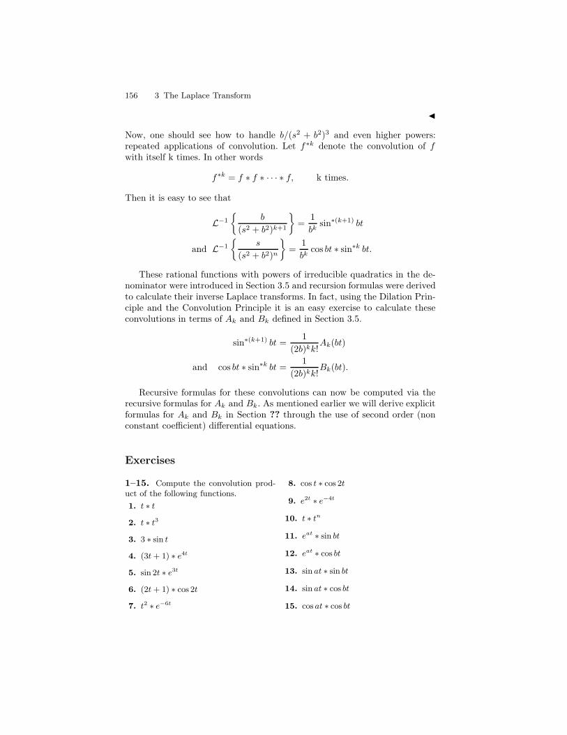
156 3 The Laplace Transform
J
Now, one should see how to handle b/(s2 + b2)3 and even higher powers:repeated applications of convolution. Let f∗k denote the convolution of fwith itself k times. In other words
f∗k = f ∗ f ∗ · · · ∗ f, k times.
Then it is easy to see that
L−1
b
(s2 + b2)k+1
=1
bksin∗(k+1) bt
and L−1
s
(s2 + b2)n
=1
bkcos bt ∗ sin∗k bt.
These rational functions with powers of irreducible quadratics in the de-nominator were introduced in Section 3.5 and recursion formulas were derivedto calculate their inverse Laplace transforms. In fact, using the Dilation Prin-ciple and the Convolution Principle it is an easy exercise to calculate theseconvolutions in terms of Ak and Bk defined in Section 3.5.
sin∗(k+1) bt =1
(2b)kk!Ak(bt)
and cos bt ∗ sin∗k bt =1
(2b)kk!Bk(bt).
Recursive formulas for these convolutions can now be computed via therecursive formulas for Ak and Bk. As mentioned earlier we will derive explicitformulas for Ak and Bk in Section ?? through the use of second order (nonconstant coefficient) differential equations.
Exercises
1–15. Compute the convolution prod-uct of the following functions.
1. t ∗ t
2. t ∗ t3
3. 3 ∗ sin t
4. (3t + 1) ∗ e4t
5. sin 2t ∗ e3t
6. (2t + 1) ∗ cos 2t
7. t2 ∗ e−6t
8. cos t ∗ cos 2t
9. e2t ∗ e−4t
10. t ∗ tn
11. eat ∗ sin bt
12. eat ∗ cos bt
13. sin at ∗ sin bt
14. sin at ∗ cos bt
15. cos at ∗ cos bt
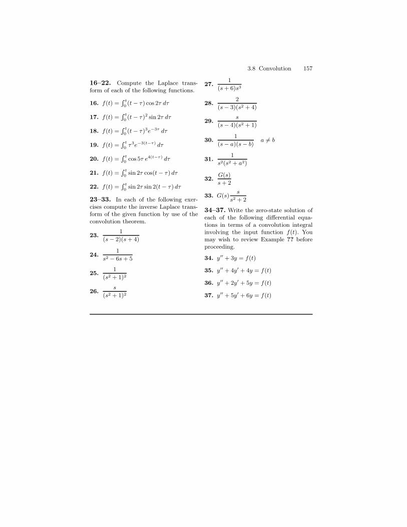
3.8 Convolution 157
16–22. Compute the Laplace trans-form of each of the following functions.
16. f(t) = t
0(t − τ ) cos 2τ dτ
17. f(t) = t
0(t − τ )2 sin 2τ dτ
18. f(t) = t
0(t − τ )3e−3τ dτ
19. f(t) = t
0τ 3e−3(t−τ) dτ
20. f(t) = t
0cos 5τ e4(t−τ) dτ
21. f(t) = t
0sin 2τ cos(t − τ ) dτ
22. f(t) = t
0sin 2τ sin 2(t − τ ) dτ
23–33. In each of the following exer-cises compute the inverse Laplace trans-form of the given function by use of theconvolution theorem.
23.1
(s − 2)(s + 4)
24.1
s2 − 6s + 5
25.1
(s2 + 1)2
26.s
(s2 + 1)2
27.1
(s + 6)s3
28.2
(s − 3)(s2 + 4)
29.s
(s − 4)(s2 + 1)
30.1
(s − a)(s − b)a 6= b
31.1
s2(s2 + a2)
32.G(s)
s + 2
33. G(s)s
s2 + 2
34–37. Write the zero-state solution ofeach of the following differential equa-tions in terms of a convolution integralinvolving the input function f(t). Youmay wish to review Example ?? beforeproceeding.
34. y′′ + 3y = f(t)
35. y′′ + 4y′ + 4y = f(t)
36. y′′ + 2y′ + 5y = f(t)
37. y′′ + 5y′ + 6y = f(t)
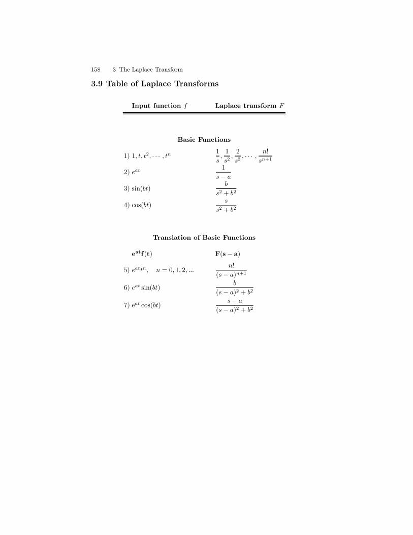
158 3 The Laplace Transform
3.9 Table of Laplace Transforms
Input function f Laplace transform F
Basic Functions
1) 1, t, t2, · · · , tn 1
s,
1
s2,
2
s3, · · · , n!
sn+1
2) eat 1
s− a3) sin(bt)
b
s2 + b2
4) cos(bt)s
s2 + b2
Translation of Basic Functions
eatf(t) F(s− a)
5) eattn, n = 0, 1, 2, ...n!
(s− a)n+1
6) eat sin(bt)b
(s− a)2 + b2
7) eat cos(bt)s− a
(s− a)2 + b2
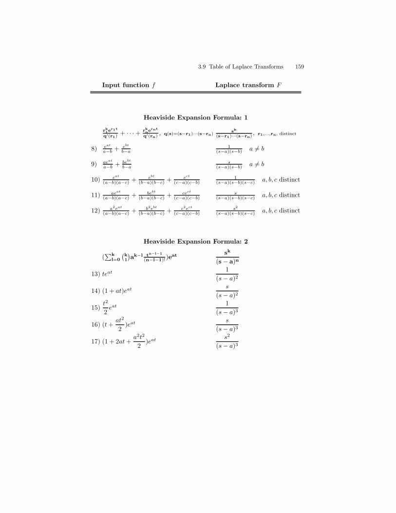
3.9 Table of Laplace Transforms 159
Input function f Laplace transform F
Heaviside Expansion Formula: 1
rk1er1t
q′(r1) + · · ·+ rknernt
q′(rn) , q(s)=(s−r1)···(s−rn)sk
(s−r1)···(s−rn) , r1,...,rn, distinct
8) eat
a−b + ebt
b−a1
(s−a)(s−b) a 6= b
9) aeat
a−b + bebt
b−as
(s−a)(s−b) a 6= b
10) eat
(a−b)(a−c) + ebt
(b−a)(b−c) + ect
(c−a)(c−b)1
(s−a)(s−b)(s−c) a, b, c distinct
11) aeat
(a−b)(a−c) + bebt
(b−a)(b−c) + cect
(c−a)(c−b)s
(s−a)(s−b)(s−c) a, b, c distinct
12) a2eat
(a−b)(a−c) + b2ebt
(b−a)(b−c) + c2ect
(c−a)(c−b)s2
(s−a)(s−b)(s−c) a, b, c distinct
Heaviside Expansion Formula: 2
(∑k
l=0
(
k
l
)
ak−l tn−l−1
(n−l−1)!)eat
sk
(s− a)n
13) teat 1
(s− a)2
14) (1 + at)eat s
(s− a)2
15)t2
2eat 1
(s− a)3
16) (t+at2
2)eat s
(s− a)3
17) (1 + 2at+a2t2
2)eat s2
(s− a)3
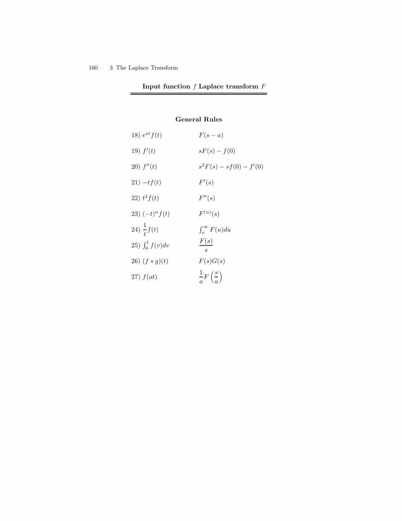
160 3 The Laplace Transform
Input function f Laplace transform F
General Rules
18) eatf(t) F (s− a)
19) f ′(t) sF (s)− f(0)
20) f ′′(t) s2F (s)− sf(0)− f ′(0)
21) −tf(t) F ′(s)
22) t2f(t) F ′′(s)
23) (−t)nf(t) F (n)(s)
24)1
tf(t)
∫∞s F (u)du
25)∫ t
0f(v)dv
F (s)
s
26) (f ∗ g)(t) F (s)G(s)
27) f(at)1
aF( s
a
)
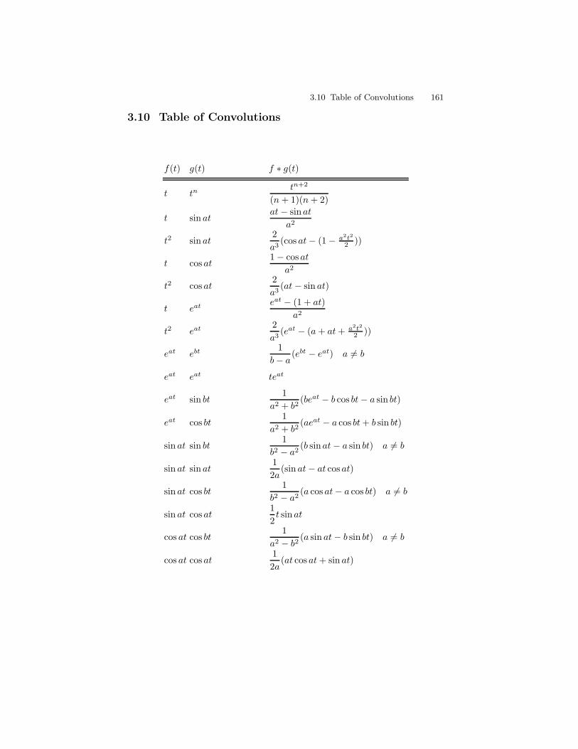
3.10 Table of Convolutions 161
3.10 Table of Convolutions
f(t) g(t) f ∗ g(t)
t tntn+2
(n+ 1)(n+ 2)
t sin atat− sinat
a2
t2 sin at2
a3(cos at− (1− a2t2
2 ))
t cos at1− cos at
a2
t2 cos at2
a3(at− sin at)
t eat eat − (1 + at)
a2
t2 eat 2
a3(eat − (a+ at+ a2t2
2 ))
eat ebt 1
b− a (ebt − eat) a 6= b
eat eat teat
eat sin bt1
a2 + b2(beat − b cos bt− a sin bt)
eat cos bt1
a2 + b2(aeat − a cos bt+ b sin bt)
sin at sin bt1
b2 − a2(b sinat− a sin bt) a 6= b
sin at sin at1
2a(sin at− at cos at)
sin at cos bt1
b2 − a2(a cos at− a cos bt) a 6= b
sin at cos at1
2t sinat
cos at cos bt1
a2 − b2 (a sin at− b sin bt) a 6= b
cos at cos at1
2a(at cos at+ sin at)

4
Linear Constant Coefficient Differential
Equations
In Section 2.2 we introduced the first order linear differential equation
a1(t)y′ + a0(t)y = f(t)
and discussed how the notion of linearity led us to a concise description of thestructure of the solution set. We also provided an algorithm for obtaining thesolution set explicitly.
In this and subsequent chapters we will consider the higher order lineardifferential equations and, in the second order case, consider applications tomechanical and electrical problems and wave oscillations. Again, the notion oflinearity is of fundamental importance for it implies a rather simple structureof the solution set. Unfortunately, unlike the first order case, there is no generalsolution method, except when the coefficients are constant. It is for this reasonthat in this chapter we focus on the important case of constant coefficientlinear differential equations. Many important physical phenomena are modeledby linear constant coefficient differential equations. In chapter 6 we considerthe situation where the coefficients are functions. Much of the general theorywe discuss here will carry over. In chapter 7 we will consider power seriesmethods for solving such.
4.1 Notation and Definitions
Suppose a0, . . . , an are scalars, an 6= 0, and f is a function defined on someinterval I. A differential equation of the form
any(n) + an−1y
(n−1) + · · ·+ a1y′ + a0y = f(t), (1)
is called a constant coefficient nth order linear differential equation.The constants a0, . . . , an are called the coefficients and an is called the lead-ing coefficient. By dividing by an, if necessary, we can assume that theleading coefficient is 1. We will frequently make this assumption; there is no
164 4 Linear Constant Coefficient Differential Equations
loss in generality. When the leading coefficient is 1 the function f is calledthe forcing function. When f = 0, we call Equation (1) homogeneous,otherwise, it is called nonhomogeneous.
Example 1. Consider the following list of differential equations.
1. 3y′′ + 2y′ − 5y = 0
2. y′′ − y′=0
3. y′′ − 4y = 0
4. y′′′ + y′ + y = t
5. 4y′ + y = 1
6. y(4) + 4ty = 1t
Examples (1.1) to (1.5) are constant coefficient linear differential equations.The presence of 4t in front of the y term makes Example (1.6) non constantcoefficient. Examples (1.1) to (1.3) are homogeneous while the others arenonhomogeneous. Examples (1.1) to (1.3) are second order, Example (1.4) isthird order, Example (1.5) is first order, and Example(1.6) is fourth order.
The left hand side of Equation (1) is made up of a linear combination ofdifferentiations and multiplications by constants. Let D denote the deriva-tive operator: D(y) = y′. If Cn(I) denotes the set of functions that have acontinuous nth derivative on the interval I then D : Cn(I) → Cn−1(I). Weare using the convention that C0(I) is the set of continuous functions on theinterval I. In a similar way D2 will denote the second derivative operator.Thus D2(y) = y′′ and D2 : Cn(I)→ Cn−2(I). Let
L = anDn + · · ·+ a1D + a0, (2)
where a0, . . . an are the same constants given in Equation (1). Then L(y) =any
(n) + · · ·+ a1y′ + a0y and Equation (1) can be rewritten
L(y) = f.
For example, y′′+2y′+y can be rewritten Ly where L = D2 +2D+1.We callL in Equation (2) a linear constant coefficient differential operator oforder n, (assuming, of course, that an 6= 0). Since L is a linear combinationof powers of D we will sometimes refer to it as a polynomial differentialoperator. More specifically, if
q(s) = ansn + an−1s
n−1 + · · ·+ a1s+ a0,
then q is a polynomial of order n and L is obtained from q by substitutingD for s and we will write L = q(D). The polynomial q is referred as thecharacteristic polynomial of L. The operator L can be thought of as tak-ing a function y that has at least n continuous derivatives and producing acontinuous function.
Example 2. Suppose L = D2 − 4D + 3. Find
L(tet), L(et), and L(e3t)
.
4.1 Notation and Definitions 165
I Solution.
• L(tet) = D2(tet)− 4D(tet) + 3(tet)= D(et + tet)− 4(et + tet) + 3tet
= 2et + tet − 4et − 4tet + 3tet
= −2et.
• L(et) = D2(et)− 4D(et) + 3(et)= et − 4et + 3et
= 0.
• L(e3t) = D2(e3t)− 4D(e3t) + 3(e3t)= 9e3t − 12e3t + 3e3t
= 0.J
Example 3. Suppose L = D3 + D. Find
L(sin t), L(1), and L(et)
I Solution.
• L(sin t) = D3(sin t) + D(sin t)= cos t− cos t= 0.
• L(1) = D3(1) + D(1)= 0.
• L(et) = D3(et) + D(et)= (et) + (et)= 2et.
J
In each case, L takes a function and produces a new function. The casewhere that new function is identically 0 is important as we will see below.
Linearity
The adjective ‘linear’ describes a very important property that L satisfies. Toexplain this let’s start with the familiar derivative operator D. One learnsearly on in calculus the following two properties:
1. If y1 and y2 are continuously differentiable functions then
D(y1 + y2) = D(y1) + D(y2).
2. If y is a continuously differentiable function and c is a scalar then
D(cy) = cD(y).
166 4 Linear Constant Coefficient Differential Equations
Simply put, D preserves addition and scalar multiplication of functions. Whenan operation on functions satisfies these two properties we call it linear.Observe closely the following proposition.
Proposition 4. The operator
L = anDn + . . .+ a1D + a0
given by Equation 2 is linear. Specifically,
1. If y1 and y2 have sufficiently many derivatives then
L(y1 + y2) = L(y1) + L(y2).
2. If y has sufficiently many derivatives and c is a scalar then
L(cy) = cL(y).
Proof. Suppose y, y1, and y2 are n-times differentiable functions and c is ascalar. If k ≤ n then by induction we have
Dk(y1 + y2) = Dk−1(Dy1 + Dy2) = Dky1 + Dky2.
Also by induction, if c is a scalar we have
Dk(cy) = Dk−1D(cy) = Dk−1cD(y) = cDk(y). (3)
Thus Dk is linear. We also observe that multiplication by a constant ak like-wise preserves multiplication and addition. We thus have
L(y1 + y2) = anDn(y1 + y2) + · · ·+ a1D(y1 + y2) + a0(y1 + y2)
= an(Dny1 + Dny2) + · · ·+ a1(Dy1 + Dy2) + a0(y1 + y2)
= anDny1 + · · ·+ a1Dy1 + a0y1 + anDny2 + · · ·+ a1Dy2 + a0y2
= Ly1 + Ly2.
Thus L preserves addition. In a similar way L preserves scalar multiplicationand hence is linear.
To illustrate the power of linearity consider the following example.
Example 5. Let L = D2 − 4D + 3. Use linearity to determine
L(3et + 4tet + 5e3t).
I Solution. Recall from Example 2 that
• L(et) = 0
• L(tet) = −2et.• L(e3t) = 0.
Using linearity we obtain
L(3et + 4tet + 5e3t) = 3L(et) + 4L(tet) + 5L(e3t)
= 3 · 0 + 4 · (−2et) + 5 · 0= −8et.
J
4.1 Notation and Definitions 167
Solutions
A solution to Equation (1) is a function y defined on some interval I withsufficiently many continuous derivatives so that Ly = f . The solution set orthe general solution is the set of all solutions.
Linearity is particulary useful for finding solutions in the homogeneouscase. The following proposition shows that linear combinations of known so-lutions produce new ones.
Proposition 6. Suppose L is a linear differential operator then the solutionset to Ly = 0 is a linear space. Specifically, suppose y1 and y2 are solutionsto Ly = 0. Then c1y1 + c2y2 is a solution to Ly = 0 for all scalars c1 and c2.
Proof. By Proposition 4 we have
L(c1y1 + c2y2) = c1L(y1) + c2L(y2)
= c1 · 0 + c2 · 0 = 0.
utExample 7. Use Example 2 to find homogeneous solutions to Ly = 0, where
L = D2 − 4D + 3
I Solution. In Example 2 we found that L(et) = 0 and L(e3t) = 0. Nowusing Proposition 6 we have
c1et + c2e
3t
is a solution to Ly = 0, for all scalars c1 and c2. In other words,
L(c1et + c2e
3t) = 0,
for all scalars c1 and c2. We will later show that all of the homogeneoussolutions are of this form. J
We cannot underscore more the importance of Proposition 6. Once a fewspecific solutions to Ly = 0 are known then all linear combinations are likewisesolutions.
Given a constant coefficient linear differential equation Ly = f we callLy = 0 the associated homogeneous differential equation. The followingtheorem considers the nonhomogeneous case. Note it carefully.
Theorem 8. Suppose L is a linear differential operator and f is a continuousfunction. If yp is a fixed particular solution to Ly = f and yh is any solutionto the associated homogeneous differential equation Ly = 0 then
yp + yh
is a solution to Ly = f . Furthermore, any solution y to Ly = f has the form
y = yp + yh.
168 4 Linear Constant Coefficient Differential Equations
Proof. Suppose yp satisfies Lyp = f and yh satisfies Lyh = 0. Then by linearity
L(yp + yh) = Lyp + Lyh = f + 0 = f.
Thus yp + yh is a solution to Ly = f . On the other hand, suppose y is anysolution to Ly = f . Let yh = y − yp. Then, again by linearity,
Lyh = L(y − yp) = Ly − Lyp = f − f = 0.
Thus yh is a solution to Ly = 0 and y = yp + yh. ut
This important theorem actually provides an effective strategy for findingthe solution set to a linear differential equation:
Algorithm 9. The general solution to a linear differential equation
Ly = f
can be found as follows:
1. Find all the solutions to the associated homogeneous differential equationLy = 0,
2. Find one particular solution yp,
3. Add the particular solution to the homogeneous solutions:
yp + yh.
As yh varies over all homogeneous solution we obtain all solution to Ly =f .
This is the strategy we will follow. Section 4.3 will be devoted to determiningsolutions to the associated homogeneous differential equation. Sections 4.4and 4.5 will show methods for finding a particular solution.
Example 10. Use Algorithm 9 and Example 3 to find solutions to
y′′′ + y′ = 2et.
I Solution. The left-hand side can be written Ly, where L is the differentialoperator
L = D3 +D.
From Example 3 we found
• L(et) = 2et,
• L(sin t) = 0,
• L(1) = 0
4.1 Notation and Definitions 169
Notice that the first equation tells us that a particular solution is yp = et.The second and third equations give sin t and 1 as solutions to the associ-ated homogeneous differential equation Ly = 0. Thus, by Proposition 6, foreach scalar c1 and c2, the function yh = c1 sin t + c2(1) = c1 sin t + c2 is ahomogeneous solution for all scalars c1, c2 ∈ R. Now, by Theorem 8 we have
yp + yh = et + c1 sin t+ c2
is a solution to Ly = 2et, for all scalars c1 and c2. At this point we cannotsay that this is the solution set. In fact, there are other solutions that we willlater find. J
Initial Value Problems
Suppose L is a constant coefficient linear differential operator of order n andf is a function defined on an interval I. Let t0 ∈ I. To the equation
Ly = f
we can associate initial conditions of the form
y(t0) = y1, y′(t0) = y1, . . . , y
(n−1)(t0) = yn−1.
We refer to the initial conditions and the differential equation Ly = f as aninitial value problem, just as in the first order case. In some applicationsy(t0) represents initial position, y′(t0) represents initial velocity, and y′′(t0)represents initial acceleration.
After finding the general solution the initial conditions are used to deter-mine the arbitrary constants that appear. Consider the following example.
Example 11. Use Example 2 to find the solution to the following initialvalue problem
Ly = −2et, y(0) = 1, y′(0) = −2,
where L = D2 − 4D + 3
I Solution. In Example 2 we verified
• L(tet) = −2et,
• L(et) = 0,
• L(e3t) = 0.
Linearity givesy = tet + c1e
t + c2e3t,
is a solution to Ly = −2et for every c1, c2 ∈ R. We will later show all of thesolutions are of this form. Observe that y′ = et + tet + c1e
t + 3c2e3t. Setting
t = 0 in both y and y′ gives
170 4 Linear Constant Coefficient Differential Equations
1 = y(0) = c1 + c2
−2 = y′(0) = 1 + c1 + 3c2.
Solving these equations gives c1 = 3, and c2 = −2. Thus y = tet + 3et − 2e3t
is a solution to the given initial value problem. It turns out that y is the onlysolution to this initial value problem. Uniqueness of solutions to initial valueproblems is the subject of our next section.
Exercises
1-10 Determine which of the followingare constant coefficient linear differentialequations. In these cases write the equa-tion is the form Ly = f , determine theorder, the characteristic polynomial, andwhether they are homogeneous.
1. y′′ − yy′ = 6
2. y′′′ − 3y′ = et
3. y′′′ + y′ + 4y = 0
4. y′′ + sin(y) = 0
5. ty′ + y = ln t
6. y′′ + 2y′ = et
7. y′′ − 7y′ + 10t = 0
8. y′ + 8y = t
9. y′′ + 2 = cos t
10. 2y′′ − 12y′ + 18y = 0
11-16: For the linear operator L, deter-mine L(y).
11. L = D2 + 3D + 2.(a) y = et
(b) y = e−t
(c) y = sin t
12. L = D2 − 2D + 1.(a) y = 4et
(b) y = cos t(c) y = −e2t
13. L = D − 2.(a) y = e−2t
(b) y = 3e2t
(c) y = tan t
14. L = D2 + 1.(a) y = −4 sin t(b) y = 3 cos t(c) y = 1
15. L = D3 − 4D.(a) y = e2t
(b) y = e−2t
(c) y = 2
16. L = D2 − 4D + 8.(a) y = e2t
(b) y = e2t sin 2t(c) y = e2t cos 2t
17. Suppose L = D2 − 5D + 4. Verifythat• L(cos 2t) = 10 sin 2t
• L(et) = 0
• L(e4t) = 0,and use this information to findother solutions to Ly = 10 sin 2t.
18. Suppose L = D2−D−6. Verity that• L(te3t) = 5e3t
• L(e3t) = 0
• L(e−2t) = 0and use this information to findother solutions to Ly = 5e3t.
19. Suppose L = D3 − 4D. Verity that• L(te2t) = 8e2t
4.2 The Existence and Uniqueness Theorem 171
• L(e2t) = 0• L(e−2t) = 0• L(1) = 0and use this information to findother solutions to Ly = 8e2t.
20. Suppose L = D4 − 16. Verity that• L(sin t) = −15 sin t• L(e2t) = 0• L(e−2t) = 0• L(sin 2t) = 0• L(cos 2t) = 0and use this information to findother solutions to Ly = −15 sin t.
21. Let L be as in Exercise 17. Use theresults there to solve the initial valueproblem
Ly = 10 sin 2t,
where y(0) = 1 and y′(0) = −3.
22. Let L be as in Exercise 18. Use theresults there to solve the initial valueproblem
Ly = 5e3t,
where y(0) = −1 and y′(0) = 8.
23. Let L be as in Exercise 19. Use theresults there to solve the initial valueproblem
Ly = 8e2t,
where y(0) = 2, y′(0) = 7, andy′′(0) = 0.
24. Let L be as in Exercise 20. Use theresults there to solve the initial valueproblem
Ly = −15 sin t,
where y(0) = 0, y′(0) = 3, y′′(0) =−16, and y′′′(0) = −9.
4.2 The Existence and Uniqueness Theorem
In this section we prove a fundamental theorem for this chapter: The Exis-tence and Uniqueness Theorem for constant coefficient linear differentialequations. Its statement follows.
Theorem 1 (The Existence and Uniqueness Theorem). Suppose p isan nth-order real polynomial, L = p(D), and f is a continuous real-valuedfunction on an interval I. Let t0 ∈ I. Then there is a unique real-valuedfunction y defined on I satisfying
Ly = f y(t0) = y0, y′(t0) = y1, . . . , y
(n−1)(t0) = yn−1 (1)
where y0, y1, . . . , yn−1 ∈ R. If I ⊃ [0,∞) and f has a Laplace transformthen so does the solution y. Furthermore, if f is in E then y is in E.
You will notice in the statement that when f has a Laplace transform sodoes the solution. This theorem thus justifies the use of the Laplace transformmethod in Section 3.6. Specifically, when we considered a differential equationof the form Ly = f and applied the Laplace transform we implicitly assumedthat y, the solution, was in the domain of the Laplace transform. This theoremnow establishes this when the forcing function f has a Laplace transform.
172 4 Linear Constant Coefficient Differential Equations
The proof of this theorem is by induction on the order of L. The mainidea is to factor L = p(D) into linear terms and use what we know about firstorder linear differential equations. Consider, for example, L = D2 − 3D + 2.The characteristic polynomial is q(s) = s2 − 3s + 2 and factors as q(s) =(s− 1)(s− 2). Observe,
(D − 1)(D − 2)y = (D − 1)(y′ − 2y)
= (D − 1)y′ − (D − 1)(2y)
= y′′ − y′ − (2y′ − 2y)
= y′′ − 3y′ + 2y
= (D2 − 3D + 2)y = q(D)y.
Therefore q(D) = (D − 1)(D − 2) and since there was nothing special aboutthe order we can also write q(D) = (D−2)(D−1). The key observation whythis factorization works in this way is that the coefficients are scalars and notfunctions. (The latter case will be considered in Chapter 6.) More generally, if apolynomial, q, factors as q(s) = q1(s)q2(s) then the corresponding differentialoperator, q(D), factors as q(D) = q1(D)q2(D).
To get a feel for the inductive proof consider the following example.
Example 2. Solve the second order differential equation
y′′ − 3y′ + 2y = et, y(0) = 0, y′(0) = 1. (2)
I Solution. Let L = D2 − 3D + 2. Then L = (D− 1)(D− 2), as discussedabove. The differential equation in Equation (2) can now be written in theform
(D− 1)(D− 2)y = et. (3)
Letu = (D− 2)y = y′ − 2y. (4)
Then u(0) = y′(0) − 2y(0) = 1. Substituting u into Equation (3) gives thefirst order initial value problem
(D− 1)u = et, u(0) = 1.
An easy calculation using Algorithm ?? of Chapter 2 gives u(t) = (t + 1)et.Equation (4) now gives
y′ − 2y = u = (t+ 1)et y(0) = 0.
Again an easy calculation gives y = −(t+ 2)et + 2e2t. J
Higher order differential equations are done similarly, As you well know,however, factoring a polynomial into linear terms sometimes introduces com-plex numbers. For example, s2 + 1 factors into s+ i and s− i. Hence, we will
4.2 The Existence and Uniqueness Theorem 173
need to consider complex valued functions and not just real valued functions.It is not uncommon in mathematics to achieve a desired result by provingmore than is needed. This is certainly the case here. We will end up provinga complex-valued analogue of Theorem 1 and on the way you will see theadvantage of recasting this problem in the domain of the complex numbers.
Complex-Valued Solutions
For the most part we will be concerned with a real valued function y defined onsome interval that satisfies Ly = f . However, as we indicated above, there aretimes when it is useful to consider a complex valued function z that satisfiesLz = f . Under the right circumstances complex valued solutions are morereadily obtained and one can then find real valued solutions from the complexvalued solutions. A similar idea was seen in Chapter 3 where we calculated theLaplace transform of cos t. There we introduced the complex-valued functioneit which, by Euler’s formula, has real part cos t. The Laplace transform of eit
was easy to compute and its real part gave the desired result. Likewise, thecomputation of the real standard basis Bq, for q a real polynomial, is simpleto determine via the complex standard basis Bq,C.
Suppose L is a constant coefficient linear differential operator and f(t)is a complex valued function. A complex valued solution to Lz = f is acomplex valued function z such that Lz = f . Our primary interest will bewhen L has real coefficients. However, there will be occasions when it will beconvenient and necessary to allow L to have complex coefficients. The mainresults of the previous section, i.e. linearity and its consequences, are also validover the complex numbers.
Example 3. Show that z(t) = teit is a solution to
z′′ + z = 2ieit.
I Solution. We use the product rule to compute
z′(t) = eit + iteit
and z′′(t) = 2ieit − teit.
Then we obtainz′′ + z = 2ieit − teit + teit = 2ieit.
J
Let’s discuss this example a little further. Let L = D2 +1. The coefficientsare real and hence, when we separate the differential equation Lz = z′′ + z =2ieit into its real and imaginary parts we obtain
Lx = x′′ + x = −2 sin t
Ly = y′′ + y = 2 cos t.
174 4 Linear Constant Coefficient Differential Equations
Now observe that the solution we considered, z(t) = teit, has real part x(t) =t cos t and imaginary part y(t) = t sin t. Furthermore,
Lx(t) = (t cos t)′′ + t cos t = (−2 sin t− t cos t) + t cos t = −2 sin t.
A similar calculation gives, Ly(t) = 2 cos t. Thus the real and imaginary partsof z(t) = teit satisfy, respectively, the equations above. The following theoremtells us that this happens more generally.
Theorem 4. Suppose L = q(D), where q is a polynomial with real coefficients.Suppose f(t) = α(t)+ iβ(t) is a complex valued function and z(t) is a complexvalued solution to
Lz = f.
If x(t) and y(t) are the real and imaginary parts of z(t) then x(t) satisfies
Lx = α
and y(t) satisfiesLy = β.
Proof. Since Dkz = Dkx+iDky the real part of Dkz is Dkx and the imaginarypart is Dky. Now suppose ak is a real number then
akDkz = akD
kx+ iakDky;
the real part is akDkx and the imaginary part is akD
ky. From this it followsthat the real part of Lz is Lx and the imaginary part is Ly. Since Lz = α+ iβand since two complex valued functions are equal if and only if their real andcomplex parts are equal we have
Lx = α
andLy = β.
ut
Remark 5. It is an essential hypothesis that q be a real polynomial. Do yousee where we used this assumption in the proof? Exercises 13-15 explore byexamples what can be said when q is not real.
The First Order Case
We begin the proof of Existence and Uniqueness Theorem by expanding thefirst order case established in Section ?? to include complex valued functions.
4.2 The Existence and Uniqueness Theorem 175
Theorem 6 (First Order). Suppose f is a continuous complex valued func-tion on an interval I. Let t0 ∈ I and γ ∈ C. Then there is a unique complexvalued function z on I satisfying
z′ + γz = f z(t0) = z0 ∈ C. (5)
If I ⊃ [0,∞) and f has a Laplace transform then so does the solution y.Furthermore, if f is in EC then z ∈ EC.
Proof. The proof of this theorem follows the same line of thought given inTheorem ?? and Corollaries ??. Suppose z is a solution to the initial valueproblem given in 5. Using the integrating factor eγt we get
(eγtz)′ = eγtf.
Integrating both sides gives
eγtz(t) =
∫ t
t0
eγxf(x) dx+ C
and hence
z(t) = e−γt
∫ t
t0
eγxf(x) dx + e−γtC.
The initial condition z(t0) = z0 implies that C = eγt0z0 and we arrive at theformula
z(t) = e−γt
∫ t
t0
eγxf(x) dx + e−γ(t−t0)z0. (6)
Since a solution must be expressed by this formula, it must be unique. Fur-thermore, it is a simple exercise to show that this formula defines a solution,thus proving existence. Now suppose the domain of f includes [0,∞) and fhas a Laplace transform. The First Translation Principle, Theorem 3.1.12,implies that eγtf(t) has a Laplace transform and Theorem ?? implies that itsantiderivative has a Laplace transform. The formula for z in Equation (5) ismade up of a sequence of such operations applied to f . It follows then that zhas a Laplace transform. Furthermore, if f ∈ EC a similar argument impliesz ∈ EC. ut
There is little value in memorizing Equation 6. To find a solution in thecomplex-valued case it is easier to follow Algorithm ??, given earlier in thereal case.
Example 7. Find the solution to
z′ − iz = 1 z(0) = 1 + i.
176 4 Linear Constant Coefficient Differential Equations
I Solution. Observe that since f(t) = 1 is in EC Theorem 6 implies that thesolution is in EC. Indeed, the integrating factor is e −i dt = e−it. Multiplyingby the integrating factor gives
(e−itz)′ = e−it.
Integration gives
e−itz =e−it
−i + C
= ie−it + C.
Hence,z = i+ Ceit ∈ EC.
The initial condition z(0) = 1 + i implies that C = 1 and we thus obtain thesolution
z = i+ eit = cos t+ i(1 + sin t).
J
The General Case
We proceed by induction to prove the Existence and Uniqueness theorem forcomplex-valued functions.
Theorem 8. Suppose p is an nth order complex valued polynomial and f is acontinuous complex valued function on an interval I. Let t0 ∈ I. Then thereis a unique complex valued function z satisfying
p(D)z = f z(t0) = z0, z′(t0) = z1, . . . , z
(n−1)(t0) = zn−1 (7)
where z0, z1, . . . , zn−1 ∈ C. If I ⊃ [a,∞) and f has a Laplace transformthen so does the solution z. Furthermore, if f is in EC then z ∈ EC.
Proof. We may assume p has leading coefficient one. Over the complex num-bers p has a root γ ∈ C and thus factors as p(s) = (s − γ)p1(s), where p1(s)is a polynomial of degree n− 1. We can write
p(D) = (D − γ)p1(D).
Suppose p1(s) = sn−1 + an−2sn−2 + · · · + a1s + a0. Consider the differential
equation
(D − γ)u = f u(t0) = zn−1 + an−2zn−2 + · · ·+ a1z1 + a0z0.
Theorem 6 implies there is a unique solution u. Now consider the differentialequation
4.2 The Existence and Uniqueness Theorem 177
p1(D)z = u z(t0) = z0, z′(t0) = z1, . . . , z
(n−2)(t0) = zn−2.
By induction there is a unique solution z. Now observe that
p(D)z = (D − γ)p1(D)z = (D − γ)u = f.
Furthermore,
z(n−1)(t0) = (Dn−1 − p1(D))z(t0) + p1(D)z(t0)
= −(an−2Dn−2 + · · ·+ a1D + a0)z(t0) + p1(D)z(t0)
= −(an−2zn−2 + · · ·+ a0z0) + u(t0) = zn−1.
Therefore z is a solution to Equation 7 and this proves existence. If the domainof f includes [0,∞) and f has a Laplace transform, by induction, so does uand hence so does z, by Theorem 6. Further, if f ∈ EC so is u, by induction,and again z ∈ EC, by Theorem 6.
Now suppose w is another solution to Equation 7. Let v = p1(D)w. Then(D − γ)v = (D − γ)p1(D)w = f and v(t0) = p1(D)w(t0) = Dn−1w(t0) +an−2D
n−1w(t0) + · · ·+ a1Dw(t0) + a0w(t0) = zn−1 + an−1zn−1 + · · ·+ a0z0.Thus v and u satisfy the same (n − 1)st order initial value problem and byinduction are equal. Therefore p1(D)w = u and w′(t0) = z0. Thus z and wsatisfy the same first order initial value problem and again, by the uniquenesspart of Theorem 6, we have w = z. ut
The existence and uniqueness theorem, Theorem 1, that we stated at thebeginning of this section now follows from Theorems 4 and 8.
To illustrate the inductive proof we provide the following second orderexample for which the complex numbers naturally arise. The student is askedto work out the first order initial value problems that arise. Keep in mind thatwe will provide far more efficient methods in the sections to come.
Example 9. Solve the following initial problem
y′′ + y = sin t, y(0) = 0, y′(0) = 1.
I Solution. Notice that all values are real and sin t is defined on the interval(−∞,∞). Theorem 1 tells us that there is a unique real-valued solution on(−∞,∞). Notice that sin t is the imaginary part of eit. We will consider thecomplex-valued differential equation
z′′ + z = eit, z(0) = 0, z′(0) = i. (8)
Theorem 4 applies and the imaginary part of the solution to Equation (8) isthe solution to Example 9. Let L = D2 + 1 = (D − i)(D + i). Equation (8)can be written
(D− i)(D + i)z = eit.
178 4 Linear Constant Coefficient Differential Equations
Let u = (D + i)z. Then u(0) = Dz(0) = iz(0) = i. We now solve the firstorder initial value problem
(D− i)u = eit, u(0) = i,
and get u(t) = (t+ i)eit, (see Exercise 7). Now that u is determined we returnto u = (D + i)z and determine z. The first order equation is
(D + i)z = (t+ i)eit, z(0) = 0
and the solution is
z(t) =3− 2it
4eit,
(see Exercise 8). The imaginary part is
y(t) =3
4sin t− t
2cos t
and this gives the solution we seek. J
Exercises
1-6 Use the inductive method, as illus-trated in Example 2, to solve each initialvalue problem.
1. y′′+y′−6y = 2et, y(0) = 1, y′(0) = 1
2. y′′−7y′+12y = 0, y(0) = 2,y′(0) = 7
3. y′′−2y′ +y = et, y(0) = 1, y′(0) = 0
4. y′′ + y = t, y(0) = 1, y′(0) = 1
5. y′′−2y′+2y = 0, y(0) = 0, y′(0) = 1
6. y′′′ − y′ = 1, y(0) = 1, y′(0) = −2,y′′(0) = −1.
7-10 Solve each initial value problem.
7. z′ − iz = eit, z(0) = i
8. z′ + iz = (t + i)eit, z(0) = 0
9. z′ − 3iz = sin t, z(0) = 1
10. z′′ + iz′ = 1, z(0) = 1, z′(0) = i
11. Let γ be a complex number. Showthat
d
dteγt = γeγt.
12. Let f and g be two complex-valued differential functions. Provethe product and quotient rules,namely,
(fg)′ = f ′g + g′f
and f
g ′
=f ′g − g′f
g2.
13-15 (Systems of DifferentialEquations): Suppose x and y are real-valued functions. A system of differen-tial equations consists of two differentialequations of the form
x′(t) = ax(t) + by(t) + f(t)
y′(t) = cx(t) + dy(t) + g(t),
where a, b, c, and d, are real numbersand f and g are real-valued functions.A solution is a pair of functions x andy that satisfy both equations simultane-ously. In Chapter 10 we will discuss thistopic thoroughly.
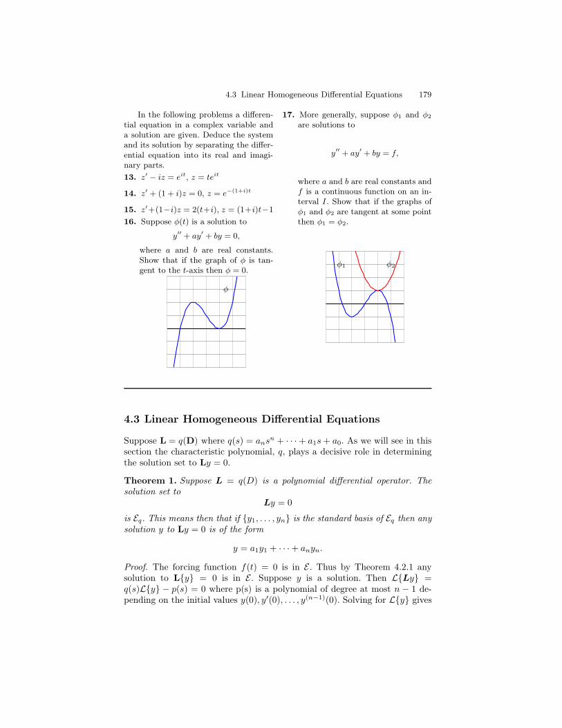
4.3 Linear Homogeneous Differential Equations 179
In the following problems a differen-tial equation in a complex variable anda solution are given. Deduce the systemand its solution by separating the differ-ential equation into its real and imagi-nary parts.
13. z′ − iz = eit, z = teit
14. z′ + (1 + i)z = 0, z = e−(1+i)t
15. z′+(1−i)z = 2(t+i), z = (1+i)t−1
16. Suppose φ(t) is a solution to
y′′ + ay′ + by = 0,
where a and b are real constants.Show that if the graph of φ is tan-gent to the t-axis then φ = 0.
φ
17. More generally, suppose φ1 and φ2
are solutions to
y′′ + ay′ + by = f,
where a and b are real constants andf is a continuous function on an in-terval I . Show that if the graphs ofφ1 and φ2 are tangent at some pointthen φ1 = φ2.
φ1 φ2
4.3 Linear Homogeneous Differential Equations
Suppose L = q(D) where q(s) = ansn + · · ·+ a1s+ a0. As we will see in this
section the characteristic polynomial, q, plays a decisive role in determiningthe solution set to Ly = 0.
Theorem 1. Suppose L = q(D) is a polynomial differential operator. Thesolution set to
Ly = 0
is Eq. This means then that if y1, . . . , yn is the standard basis of Eq then anysolution y to Ly = 0 is of the form
y = a1y1 + · · ·+ anyn.
Proof. The forcing function f(t) = 0 is in E . Thus by Theorem 4.2.1 anysolution to Ly = 0 is in E . Suppose y is a solution. Then LLy =q(s)Ly − p(s) = 0 where p(s) is a polynomial of degree at most n − 1 de-pending on the initial values y(0), y′(0), . . . , y(n−1)(0). Solving for Ly gives
180 4 Linear Constant Coefficient Differential Equations
Ly(s) =p(s)
q(s)∈ Rq.
This implies y ∈ Eq. On the other hand, suppose y ∈ Eq. Then Ly(s) =p(s)q(s) ∈ Rq and
LLy(s) = q(s)p(s)
q(s)− p1(s) = p(s)− p1(s),
where p1(s) is a polynomial that depends on the initial conditions. Note, how-ever, that p(s)− p1(s) is a polynomial in R and therefore must be identically0. Thus LLy = 0 and this implies Ly = 0. ut
Example 2. Find the general solution to the following differential equa-tions:
1. y′′ + 3y′ + 2y = 02. y′′ + 2y′ + y = 03. y′′ − 6y′ + 10y = 04. y′′′ + y′ = 0
I Solution.
1. The characteristic polynomial for y′′ + 3y′ + 2y = 0 is
q(s) = s2 + 3s+ 2 = (s+ 1)(s+ 2).
The roots are −1 and −2. The standard basis for Eq is
e−t, e−2t
. Thusthe solution set is
Eq =
c1e−t + c2e
−2t : c1, c2 ∈ R
.
2. The characteristic polynomial of y′′ + 2y′ + y = 0 is
q(s) = s2 + 2s+ 1 = (s+ 1)2,
which has root s = −1 with multiplicity 2. The standard basis for Eq ise−t, te−t. The solution set is
Eq =
c1e−t + c2te
−t : c1, c2 ∈ R
.
3. The characteristic polynomial for y′′ − 6y′ + 10y = 0 is
q(s) = s2 − 6s+ 10 = (s− 3)2 + 1.
From this we see that the roots of q are 3 + i and 3 − i. The standardbasis for Eq is
e3t cos t, e3t sin t
. Thus the solution set is
Eq =
c1e3t cos t+ c2e
3t sin t : c1, c2 ∈ R
.
4.3 Linear Homogeneous Differential Equations 181
4. The characteristic polynomial for y′′′ + y′ = 0 is
q(s) = s3 + s = s(s2 + 1).
In this case the roots of q are 0, i, and −i. The standard basis for Eq is1, cos t, sin t. Thus the solution set is
Eq = c1 + c2 cos t+ c3 sin t : c1, c2, c3 ∈ R .
J
These examples show that conceptually it is a relatively easy process towrite down the solution set to a homogeneous constant coefficient linear dif-ferential equation. We codify the process in the following algorithm.
Algorithm 3. Given a constant coefficient linear differential equation Ly = 0the solution set is determined as follows:
1. Determine the characteristic polynomial, q.2. Determine the roots of q and their multiplicities. This is usually done by
factoring q.3. Use the roots to find the standard basis of Eq.4. The solution set is the set of all linear combinations of the functions in
the standard basis.
Initial Value Problems
Let q(D)y = 0 be a homogeneous constant coefficient differential equation,where deg p = n. Suppose y(t0) = y0, . . . , y
(n−1)(t0) = yn−1 are initial con-ditions. The Existence and Uniqueness Theorem 1 states there is a uniquesolution to the initial value problem. However, the general solution is a linearcombination of the n functions in the standard basis Eq. It follows then thatthe initial conditions uniquely determine the coefficients.
Example 4. Find the solution to
y′′′ − 4y′′ + 5y′ − 2y = 0 y(0) = 1, y′(0) = 2, y′′(0) = 0.
I Solution. The characteristic polynomial is q(s) = s3 − 4s2 + 5s− 2 andfactors as
q(s) = (s− 1)2(s− 2).
Here, only real roots arise. The basis for Eq is
et, tet, e2t
and the generalsolution is
y = c1et + c2te
t + c3e2t.
We first calculate the derivatives and simplify to get,
182 4 Linear Constant Coefficient Differential Equations
y(t) = c1et + c2te
t + c3e2t
y′(t) = (c1 + c2)et + c2te
t + 2c3e2t
y′′(t) = (c1 + 2c2)et + c2te
t + 4c3e2t.
To determine the coefficients c1, c2, and c3 we use the initial conditions.Evaluating at t = 0 gives
1 = y(0) = c1 + c3
2 = y′(0) = c1 + c2 + 2c3
0 = y′′(0) = c1 + 2c2 + 4c3.
Solving these equations gives c1 = 4, c2 = 4, and c3 = −3. The unique solutionis thus
y(t) = 4et + 4tet − 3e2t.
J
Complex-Valued Solutions
There is a complex-valued analogue to Theorem 1. It’s proof is essentially thesame; we will not repeat it.
Theorem 5. Suppose L = q(D) is a polynomial differential operator withcomplex coefficients. The solution set to
Lz = 0
is Eq,C. Thus if z1, . . . , zn is the standard basis of Eq,C then any solution zto Lz = 0 is of the form
z = a1z1 + · · ·+ anzn.
Example 6. Find the solution to
y′′ + 4y′ + 5y = 0 y(0) = 1, y′(0) = 1.
I Solution. The characteristic polynomial is
q(s) = s2 + 4s+ 5 = (s+ 2)2 + 1.
We see that q has complex roots γ1 = −2 + i and γ2 = −2 − i. We willapproach this problem in two different ways. First, we will used the complexbasis Bq,C. Second, we will use the real basis Bq. Each have their particularadvantages.
Method 1 The complex basis is Bq,C = eγ1t, eγ2t. The general solution overthe complex numbers is
4.3 Linear Homogeneous Differential Equations 183
y(t) = c1eγ1t + c2e
γ2t.
We determine c1 and c2 by the initial conditions. Observe first that
y(t) = c1eγ1t + c2e
γ2t
y′(t) = c1γ1eγ1t + c2γ2e
γ2t.
The initial conditions imply
1 = y(0) = c1 + c2
1 = y′(0) = c1γ1 + c2γ2.
We solve for c1 by multiplying the first equation by γ2 and subtracting. We getγ2−1 = c1(γ2−γ1). Thus c1 = (γ2−1)/(γ2−γ1) = (−3−i)/(−2i) = (1−3i)/2.Substituting γ1 into the first equation gives c2 = 1 − c1 = (1 + 3i)/2. UsingEuler’s equation and simplifying we get
y(t) =1− 3i
2eγ1t +
1 + 3i
2eγ2t.
= e−2t(cos t+ 3 sin t)
Method 2 The real basis for Eq is Bq =
e−2t cos t, e−t sin t
. The generalsolutions over the reals is
y(t) = c1e−2t cos t+ c2e
−2t sin t,
where c1 and c2 are real. We determine c1 and c2 by the initial conditions.Observe first that
y(t) = = c1e−2t cos t+ c2e
−2t sin t
y′(t) = (−2c1 + c2)e−2t cos t+ (−c1 − 2c2)e
−2t sin t.
The initial conditions imply
1 = y(0) = c1
1 = y′(0) = −2c1 + c2
from which we find c1 = 1 and c2 = 3. The solution is thus
y = e−2t(cos t+ 3 sin t).
J
Remark 7. In the complex case, method 1, it is generally easier to computethe derivative but harder to deal with the complex entries that arise. Whilein the real case, method 2, it is generally harder to compute the derivativebut easier to deal with only the real entries the arise.
Exercises
184 4 Linear Constant Coefficient Differential Equations
1-19 Determine the solution set to thefollowing homogeneous differential equa-tions. Write your answer as a linear com-bination of functions from the standardbasis.
1. y′ − 6y = 0
2. y′ + 4y = 0
3. y′′ − y′ − 2y = 0
4. y′′ + y′ − 12y = 0
5. y′′ + 10y′ + 24y = 0
6. y′′ − 4y′ + 12y = 0
7. y′′ + 8y′ + 16y = 0
8. y′′ − 3y′ − 10y = 0
9. y′′ + 2y′ + 5y = 0
10. 2y′′ − 12y′ + 18y = 0
11. y′′ + 13y′ + 36y = 0
12. y′′ + 8y′ + 25y = 0
13. y′′ + 10y′ + 25y = 0
14. y′′ − 4y′ − 21y = 0
15. y′′′ − y = 0
16. y′′′ − 6y′′ + 12y′ − 8y = 0
17. y(4) − y = 0
18. y′′′ + 2y′′ + y′ = 0
19. y(4) − 5y′′ + 4y = 0
20-25 Solve the following initial valueproblems.
20. y′′ − y = 0, y(0) = 0, y′(0) = 1
21. y′′ − 3y′ − 10y = 0, y(0) = 5,y′(0) = 4
22. y′′ − 10y′ + 25y = 0, y(0) = 0,y′(0) = 1
23. y′′ + 4y′ + 13y = 0, y(0) = 1,y′(0) = −5
24. y′′′ + y′′ − y′ − y = 0, y(0) = 1,y′(0) = 4, y′′(0) = −1
25. y(4) − y = 0, y(0) = −1, y′(0) = 6,y′′(0) = −3, y′′′(0) = 2
4.4 The Method of Undetermined Coefficients
In Section 4.2 we discussed extensively the existence and uniqueness theo-rem for a nonhomogeneous linear differential equation. Given a polynomialdifferential operator q(D), a solution to
q(D)y = f (1)
could be ‘built up’ by factoring q and successively applying first order meth-ods. Admittedly, this procedure can be tedious. In this section we introduce amethod that exploits linearity and the fact that such solutions are in E whenthe forcing functions f is in E . The method is called the method of unde-termined coefficients. By Theorem 4.1.8, all solutions to Equation (1) areof the form
y = yp + yh,
4.4 The Method of Undetermined Coefficients 185
where yp is a fixed particular solution and yh is any homogenous solution.In Section 4.3 we found the set of solutions associated to the homogenousequation Ly = 0. The method of undetermined coefficients is a method tofind a particular solution yp.
Here is the basic idea. We suppose f ∈ E . Theorem 4.2.1 implies a solutiony = yp to Equation (1) is in E . Therefore, the form of yp is
yp = c1y1 + · · ·+ cnyn,
where each yi, i = 1, . . . n, is a simple exponential polynomial and the co-efficients c1, . . . , cn are to be determined. We call yp a test function. Themethod of undetermined coefficients can be broken into two parts. First, de-termine which exponential polynomials, y1, . . . , yn, will arise in a test function.Second, determine the coefficients, c1, . . . , cn.
Before giving the general procedure lets consider the essence of the methodin a simple example.
Example 1. Find the general solution to
y′′ − y′ − 6y = e−t.
I Solution. Let us begin by finding the solution to the associated homoge-nous equation
y′′ − y′ − 6y = 0. (2)
Observe that the characteristic polynomial is q(s) = s2−s−6 = (s−3)(s+2).Thus, the set of homogenous solutions are of the form
yh = c1e3t + c2e
−2t. (3)
Let us now find a particular solution to y′′−y′−6y = e−t. Since any particularsolution will do, consider the case where y(0) = 0 and y′(0) = 0. Since f(t) =e−t ∈ E we conclude by the Uniqueness and Existence Theorem, Theorem4.2.1, that the solution y is in E . We apply the Laplace transform to bothsides and get
q(s)Ly (s) =1
s+ 1,
Solving for Ly gives
Ly (s) =1
(s+ 1)q(s)=
1
(s+ 1)(s− 3)(s+ 2).
It follows that y ∈ Ep, where p is the polynomial p(s) = (s+ 1)(s− 3)(s+ 2).Thus
y = c1e−t + c2e
3t + c3e−2t,
for some c1, c2, c3. Observe now that c2e3t+c3e−2t is a homogeneous solution.
This means then that leftover piece yp = c1e−t is a particular solution. This is
186 4 Linear Constant Coefficient Differential Equations
the test function. Let’s now determine c1 by plugging yp into the differentialequation. First, observe that y′p = −c1e−t and y′′p = c1e
−t. Thus, Equation(2) gives
e−t = y′′p − y′p − 6yp
= c1e−t + c1e
−t − 6c1e−t
= −4c1e−t.
From this we conclude 1 = −4c1 or c1 = −1/4. Therefore
yp =−1
4e−t
is a particular solution and the general solution is obtained by adding thehomogeneous solution to it. Thus, the functions
y = yp + yh =−1
4e−t +Ae3t +Be−2t,
where A and B are real numbers, make up the set of real solutions. J
Remark 2. Let v(s) = (s+1) be the denominator of Le−t. Then v(s)q(s) =(s + 1)(s − 3)(s + 2) and the standard basis for Evq is
e−t, e3t, e−2t
. Thestandard basis for Eq is
e3t, e−2t
. Observe that yp is made up of functionsfrom the standard basis of Evq that are not in the standard basis of Eq. Thiswill always happen. The general argument is in the proof of the followingtheorem.
Theorem 3. Suppose L = q(D) is a polynomial differential operator andf ∈ E. Suppose Lf = u
v . Let Bq denote the standard basis for Eq. Then thereis a particular solution yp to
Ly = f
which is a linear combination of terms in Bqv but not in Bq.
Proof. By Theorem 4.2.1, any solution to Ly = f is in E and hence has aLaplace Transform. Thus
Lq(D) y) = Lf =u(s)
v(s)
q(s)Ly − p(s) =u(s)
v(s)by Theorem ??
Ly = =p(s)
q(s)+
u(s)
q(s)v(s)=u(s) + p(s)v(s)
q(s)v(s).
It follows that y is in Eqv and hence a linear combination of terms in Bqv.Since Bq ⊂ Bqv, we can write y = yh + yp, where yh is the linear combinationof terms in Bq and yp is a linear combination of terms in Bqv but not in Bq.Since yh is a homogenous solution it follows that yp = y − yh is a particularsolution of the required form. ut
4.4 The Method of Undetermined Coefficients 187
Theorem 3 is the basis for the following algorithm.
Algorithm 4 (The method of undetermined coefficients). Given
q(D)y = f
1. Compute the standard basis, Bq, for Eq.2. Determine v so that Lf = u
v . I.e. f ∈ Ev.3. Compute the standard basis, Bvq, for Evq.4. The test function, yp is the linear combination with arbitrary coefficients
of functions in Bvq that are not in Bq.5. The coefficients in yp are determined by plugging yp into the differential
equation q(D)y = f .6. The general solution is given by
yp + yh,
where yh ∈ Eq.
Example 5. Find the general solution to y′′ − 5y′ + 6y = 4e2t.
I Solution. The characteristic polynomial is q(s) = s2−5s+6 = (s−2)(s−3) and the standard basis for Eq is Bq =
e2t, e3t
. Since L
4e2t
= 4s−2 we
have v(s)q(s) = (s − 2)2(s − 3) and the standard basis for Evq is Bvq =
e2t, te2t, e3t
. The only function in Bvq that is not in Bq is te2t. Thereforeour test function is yp = c1te
2t. A simple calculation gives
yp = c1te2t
y′p = c1e2t + 2c1te
2t
y′′p = 4c1e2t + 4c1te
2t.
Substitution into y′′ − 5y′ + 6y = 4e2t gives
4e2t = 4c1e2t + 4c1te
2t − 5(c1e2t + 2c1te
2t) + 6(c1te2t)
= −c1e2t.
From this it follows that c1 = −4 and yp = −4te2t. The general solution isgiven by
yp = −4te2t +Ae2t +Be3t,
where A and B are real. J
Remark 6. Based on Example 1 one might have expected that the test func-tion in Example 5 would be yp = c1e
2t. But this cannot be as e2t is a ho-mogenous solution. Observe that v(s) = s − 2 and q(s) = (s − 2)(s + 3)share a common root, namely s = 2, so that the product has root s = 2with multiplicity 2. This produces te2t in the standard basis for Evq that does
188 4 Linear Constant Coefficient Differential Equations
not appear in the standard basis for Eq. In Example 1 all the roots of vqare distinct so this phenomenon does not occur. There is thus a qualitativedifference between the cases when v and q have common roots and the caseswhere they do not. However, Algorithm 4 does not distinguish this difference.It will always produce a test function that leads to a particular solution.
Example 7. Find the general solution to
y′′ − 3y′ + 2y = 2tet.
I Solution. The characteristic polynomial is q(s) = s2 − 3s + 2 = (s −1)(s− 2). Hence the standard basis for Eq is
et, e2t
. The Laplace transformof 2tet is 2/(s − 1)2. If v(s) = (s − 1)2 then v(s)q(s) = (s − 1)3(s − 2)and y ∈ Evq, which has standard basis
et, tet, t2et, e2t
. Our test functionis yp(t) = c1te
t + c2t2et. We determine c1 and c2 by plugging yp into the
differential equation. A calculation of derivatives gives
yp = c1tet + c2t
2et
y′p = c1et + (c1 + 2c2)te
t + c2t2et
y′′p = (2c1 + 2c2)et + (c1 + 4c2)te
t + c2t2et.
Substitution into y′′ − 3y′ + 2y = 2tet gives
2tet = y′′p − 3y′p + 2yp
= (−c1 + 2c2)et − 2c2te
t.
Hence, the coefficients c1 and c2 satisfy
−c1 + 2c2 = 0
−2c2 = 2.
From this we find c2 = −1 and c1 = 2c2 = −2. Hence, a particular solution is
yp = −2te−t − t2e−t
and the general solution is
y = yp + yh = −2te−t − t2e−t +Aet +Be2t.
J
Linearity is particularly useful when the forcing function f is a sum ofterms. Here is the general principle, sometimes referred to as the Superpo-sition Principle.
Theorem 8 (Superposition Principle). Suppose yp1 is a solution to Ly =f1 and yp2 is a solution to Ly = f2. Then yp1+yp2 is a solution to Ly = f1+f2.
4.4 The Method of Undetermined Coefficients 189
Proof. By linearity
L(yp1 + yp2) = L(yp1) + L(yp2) = f1 + f2.
ut
Example 9. Find the general solution to
y′′ − 5y′ + 6y = 12 + 4e2t. (4)
I Solution. Theorem 8 allows us to find a particular solution by addingtogether the particular solutions to
y′′ − 5y′ + 6y = 12 (5)
andy′′ − 5y′ + 6y = 4e2t. (6)
In both cases the characteristic polynomial is q(s) = s2−5s+6 = (s−2)(s−3).In Equation (5) the Laplace transform of 12 is 12/s. Thus v(s) = s, q(s)v(s) =s(s− 2)(s− 3), and Bqv =
1, e2t, e3t
. The test function is yp1 = c. It is easyto see that yp1 = 2. In Example 5 we found that yp2 = −4te2t is a particularsolution to Equation (6). By Theorem 8, yp = 2−4te2t is a particular solutionto Equation (4). Thus
y = 2− 4te2t +Ae2t +Be3t
is the general solution. J
There is a complex-valued analogue to Theorem 3 that is proved in exactlythe same way.
Theorem 10 (Method of Undetermined Coefficients: The complex-valued version). Suppose L = q(D) is a polynomial differential operatorand f ∈ EC. Suppose Lf = u
v . Let Bq,C denote the standard basis for Eq,C.Then there is a particular solution zp to
Lz = f
which is a linear combination of terms in Bqv,C but not in Bq,C.
Example 11. Find the general solution to
y′′ + y = cos t. (7)
I Solution. The characteristic polynomial is q(s) = s2 + 1 which has ±i asits roots. We will approach this problem in two ways. First, we view Equation(7) as a real differential equation and apply the Method of UndeterminedCoefficients (real version). Second, we solve the differential equation z′′ + z =
190 4 Linear Constant Coefficient Differential Equations
eit using the complex version, Theorem 10. The real part of that solution givesthe solution to Equation (7) by Theorem 4.
Method 1 The real basis for Eq is Bq = cos t, sin t. With v(s) = s2 + 1 asabove we find that the real basis for Evq is Bvq = cos t, sin t, t cos t, t sin t . Itfollows now that the test function is
yp(t) = c1t cos t+ c2t sin t.
To determine the coefficients first observe
yp(t) = c1t cos t+ c2t sin t
y′p(t) = c1 cos t− c1t sin t+ c2 sin t+ c2t cos t
y′′p (t) = −2c1 sin t− c1t cos t+ 2c2 cos t− c2t sin t.Plugging these formulas into y′′ + y = cos t gives
cos t = y′′ + y
= −2c1 sin t− c1t cos t+ 2c2 cos t− c2t sin t+ c1t cos t+ c2t sin t
= −c1 sin t+ 2c2 cos t.
It follows that c1 = 0 and c2 = 1/2. Therefore yp(t) = (1/2)t sin t and thegeneral solution is
y = yp + yh =1
2t sin t+A cos t+B sin t.
Method 2 We first consider the complex-valued differential equation z′′+z =eit. The standard basis for Eq,C is Bq,C =
eit, e−it
. The Laplace transformof eit is 1
s−i . Let v(s) = s2 + 1 = (s− i)(s+ i). Then v(s)q(s) = (s− i)2(s+ i)
and the standard basis for Evq,C is Bqv,C =
eit, teit, e−it
. It follows that thetest function is given by zp = cteit. To determine c observe that
zp = cteit
z′p = c(eit + iteit)
z′′p = c(2ieit − teit).
Plugging these formulas into z′′ + z = eit gives
eit = z′′p + zp
= 2iceit.
Therefore c = 12i = − i
2 and zp = − i2e
it. By Theorem 4 the real part of zp isa solution to y′′ + y = cos t. Thus yp = 1
2 t sin t. The general solution is
y = yp + yh =1
2t sin t+A cos t+B sin t.
J
4.4 The Method of Undetermined Coefficients 191
Exercises
1-14: Given q and v below determinethe test function yp for the differentialequation q(D)y = f , where Lf = u
v.
1. q(s) = s + 1 v(s) = s − 4
2. q(s) = s − 4 v(s) = s2 + 1
3. q(s) = s2 − s − 2 v(s) = s − 3
4. q(s) = s2 + 6s + 8 v(s) = s + 3
5. q(s) = s2 − 5s + 6 v(s) = s − 2
6. q(s) = s2 − 7s + 12 v(s) = (s− 4)2
7. q(s) = (s − 5)2 v(s) = s2 + 25
8. q(s) = s2 + 1 v(s) = s2 + 4
9. q(s) = s2 + 4 v(s) = s2 + 4
10. q(s) = s2 + 4s + 5 v(s) = (s − 1)2
11. q(s) = (s − 1)2 v(s) = s2 + 4s + 5
12. q(s) = s3 − s v(s) = s + 1
13. q(s) = s3 − s2 − s + 1 v(s) = s− 1
14. q(s) = s4 − 81 v(s) = s2 + 9
15-36 Find the general solution foreach of the differential equations givenbelow.
15. y′ + 6y = 3
16. y′ + y = 4e3t
17. y′ − 4y = 2e4t
18. y′ − y = 2 cos t
19. y′′ + 3y′ − 4y = e2t
20. y′′ − 3y′ − 10y = 7e−2t
21. y′′ + 2y′ + y = et
22. y′′ + 3y′ + 2y = 4
23. y′′ + 4y′ + 5y = e−3t
24. y′′ + 4y = 1 + et
25. y′′ − y = t2
26. y′′ − 4y′ + 4y = et
27. y′′ − 4y′ + 4y = e2t
28. y′′ + y = 2 sin t
29. y′′ + 6y′ + 9y = 25te2t
30. y′′ + 6y′ + 9y = 25te−3t
31. y′′ + 6y′ + 13y = e−3t cos(2t)
32. y′′ − 8y′ + 25y = 36te4t sin(3t)
33. y′′′ − y′ = et
34. y′′′ − y′ + y′ − y = 4 cos t
35. y(4) − 5y′′ + 4y = e2t
36. y(4) − y = et + e−t
37-41 Solve each of the following initialvalue problems.
37. y′′ − 5y′ − 6y = e3t, y(0) = 2,y′(0) = 1
38. y′′ + 2y′ + 5y = 8e−t, y(0) = 0,y′(0) = 8
39. y′′ + y = 10e2t, y(0) = 0, y′(0) = 0
40. y′′−4y = 2−8t, y(0) = 0, y′(0) = 5
41. y′′′ − y′′ + 4y′ − 4y = et, y(0) = 0,y′(0) = 0, y′′(0) = 0
42-51 (The Annihilator) Suppose fis a function on some interval. If v(D)f =0 for some polynomial v then we saythat f is annihilated by v(D). For ex-ample, e3t is annihilated by D − 3 andD2 − 5D + 6. (check this!) The annihi-lator of f is the polynomial differentialoperator v(D) of least degree and lead-ing coefficient 1 that annihilates f . Forexample, the annihilator of e3t is D− 3.
Find the annihilator of each function be-low.
192 4 Linear Constant Coefficient Differential Equations
42. e5t
43. te−6t
44. cos(3t)
45. e2t cos(4t)
46. t2 sin t
47. tneat
48. Show that f has an annihilator ifand only if f ∈ E .
49. Suppose f ∈ E and Lf = uv, re-
duced. Show that the annihilator off is v(D).
50. Suppose L = q(D) is a polynomialdifferential operator and y is a solu-tion to
Ly = f,
where f ∈ E . Suppose v(D) isthe annihilator of f . Show thatq(D)v(D) annihilates y. Give an ex-ample to show that q(D)v(D) is notnecessarily the annihilator of y.
51. (continued) What does knowingthat y is annihilated by q(D)v(D)tell you about the form y takes?
4.5 The Incomplete Partial Fraction Method
In this section we provide an alternate method for finding the solution set tothe nonhomogeneous differential equation
q(D)y = f, (1)
where f ∈ E . This alternate method begins with the Laplace transformmethod and exploits the efficiency of the partial fraction decomposition algo-rithm. However the partial fraction decomposition applied to Y (s) = Ly(s)is not needed to its completion. We therefore refer to this method as theIncomplete Partial Fraction Method. For purposes of illustration andcomparison to the method of undetermined coefficients let’s reconsider Ex-ample 5 of Section 4.4.
Example 1. Find the general solution to
y′′ − 5y′ + 6y = 4e2t. (2)
I Solution. Our goal is to find a particular solution yp to which we willadd the homogeneous solutions yh. Since any particular solution will do webegin by applying the Laplace transform with initial conditions y(0) = 0 andy′(0) = 0. The characteristic polynomial is q(s) = s2− 5s+ 6 = (s− 2)(s− 3)and L
4e2t
= 4/(s−2). If, as usual, we let Y (s) = Ly(s) then q(s)Y (s) =4/(s− 2) and
Y (s) =4
(s− 2)q(s)=
4
(s− 2)2(s− 3).
In the table below we compute the (s− 2)-chain for Y (s) but stop when thedenominator reduces to q(s) = (s− 2)(s+ 3).
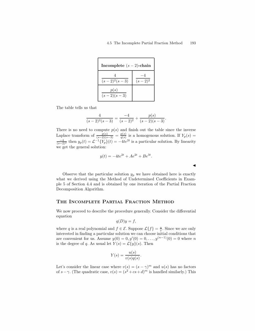
4.5 The Incomplete Partial Fraction Method 193
Incomplete (s− 2)-chain
4
(s− 2)2(s− 3)
−4
(s− 2)2
p(s)
(s− 2)(s− 3)
The table tells us that
4
(s− 2)2(s− 3)=
−4
(s− 2)2+
p(s)
(s− 2)(s− 3).
There is no need to compute p(s) and finish out the table since the inverseLaplace transform of p(s)
(s−2)(s−3) = p(s)q(s) is a homogenous solution. If Yp(s) =
−4(s−2)2 then yp(t) = L−1Yp(t) = −4te2t is a particular solution. By linearitywe get the general solution:
y(t) = −4te2t +Ae2t +Be3t.
J
Observe that the particular solution yp we have obtained here is exactlywhat we derived using the Method of Undetermined Coefficients in Exam-ple 5 of Section 4.4 and is obtained by one iteration of the Partial FractionDecomposition Algorithm.
The Incomplete Partial Fraction Method
We now proceed to describe the procedure generally. Consider the differentialequation
q(D)y = f,
where q is a real polynomial and f ∈ E . Suppose Lf = uv . Since we are only
interested in finding a particular solution we can choose initial conditions thatare convenient for us. Assume y(0) = 0, y′(0) = 0, . . . , y(n−1)(0) = 0 where nis the degree of q. As usual let Y (s) = Ly(s). Then
Y (s) =u(s)
v(s)q(s).
Let’s consider the linear case where v(s) = (s − γ)m and u(s) has no factorsof s−γ. (The quadratic case, v(s) = (s2 + cs+d)m is handled similarly.) This
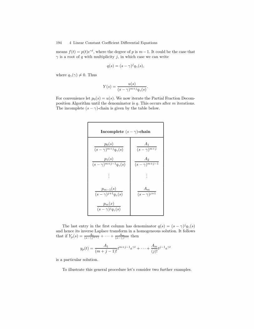
194 4 Linear Constant Coefficient Differential Equations
means f(t) = p(t)eγt, where the degree of p is m−1. It could be the case thatγ is a root of q with multiplicity j, in which case we can write
q(s) = (s− γ)jqγ(s),
where qγ(γ) 6= 0. Thus
Y (s) =u(s)
(s− γ)m+jqγ(s).
For convenience let p0(s) = u(s). We now iterate the Partial Fraction Decom-position Algorithm until the denominator is q. This occurs after m iterations.The incomplete (s− γ)-chain is given by the table below.
Incomplete (s− γ)-chain
p0(s)
(s− γ)m+jqγ(s)
A1
(s− γ)m+j
p1(s)
(s− γ)m+j−1qγ(s)
A2
(s− γ)m+j−1
......
pm−1(s)
(s− γ)j+1qγ(s)
Am
(s− γ)j+1
pm(x)
(s− γ)jqγ(s)
The last entry in the first column has denominator q(s) = (s − γ)jqγ(s)and hence its inverse Laplace transform in a homogeneous solution. It followsthat if Yp(s) = A1
(s−γ)m+j + · · ·+ Am
(s−γ)j+1 then
yp(t) =A1
(m+ j − 1)!tm+j−1eγt + · · ·+ Am
(j)!tj−1eγt
is a particular solution.
To illustrate this general procedure let’s consider two further examples.
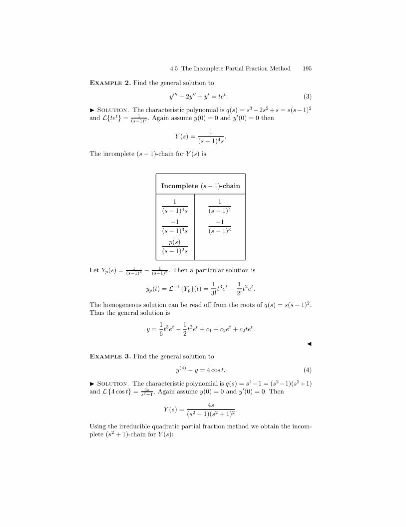
4.5 The Incomplete Partial Fraction Method 195
Example 2. Find the general solution to
y′′′ − 2y′′ + y′ = tet. (3)
I Solution. The characteristic polynomial is q(s) = s3−2s2 +s = s(s−1)2
and Ltet = 1(s−1)2 . Again assume y(0) = 0 and y′(0) = 0 then
Y (s) =1
(s− 1)4s.
The incomplete (s− 1)-chain for Y (s) is
Incomplete (s− 1)-chain
1
(s− 1)4s
1
(s− 1)4
−1
(s− 1)3s
−1
(s− 1)3
p(s)
(s− 1)2s
Let Yp(s) = 1(s−1)4 − 1
(s−1)3 . Then a particular solution is
yp(t) = L−1Yp(t) =1
3!t3et − 1
2!t2et.
The homogeneous solution can be read off from the roots of q(s) = s(s− 1)2.Thus the general solution is
y =1
6t3et − 1
2t2et + c1 + c2e
t + c2tet.
J
Example 3. Find the general solution to
y(4) − y = 4 cos t. (4)
I Solution. The characteristic polynomial is q(s) = s4−1 = (s2−1)(s2+1)and L4 cos t = 4s
s2+1 . Again assume y(0) = 0 and y′(0) = 0. Then
Y (s) =4s
(s2 − 1)(s2 + 1)2.
Using the irreducible quadratic partial fraction method we obtain the incom-plete (s2 + 1)-chain for Y (s):
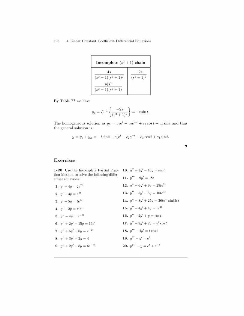
196 4 Linear Constant Coefficient Differential Equations
Incomplete (s2 + 1)-chain
4s
(s2 − 1)(s2 + 1)2−2s
(s2 + 1)2
p(s)
(s2 − 1)(s2 + 1)
By Table ?? we have
yp = L−1
−2s
(s2 + 1)2
= −t sin t.
The homogeneous solution as yh = c1et + c2e
−t + c3 cos t + c4 sin t and thusthe general solution is
y = yp + yh = −t sin t+ c1et + c2e
−t + c3 cos t+ c4 sin t.
J
Exercises
1-20 Use the Incomplete Partial Frac-tion Method to solve the following differ-ential equations.
1. y′ + 4y = 2e7t
2. y′ − 3y = e3t
3. y′ + 5y = te4t
4. y′ − 2y = t2et
5. y′′ − 4y = e−6t
6. y′′ + 2y′ − 15y = 16et
7. y′′ + 5y′ + 6y = e−2t
8. y′′ + 3y′ + 2y = 4
9. y′′ + 2y′ − 8y = 6e−4t
10. y′′ + 3y′ − 10y = sin t
11. y′′′ − 9y′ = 18t
12. y′′ + 6y′ + 9y = 25te2t
13. y′′ − 5y′ − 6y = 10te4t
14. y′′ − 8y′ + 25y = 36te4t sin(3t)
15. y′′ − 4y′ + 4y = te2t
16. y′′ + 2y′ + y = cos t
17. y′′ + 2y′ + 2y = et cos t
18. y′′′ + 4y′ = t cos t
19. y′′′ − y′ = et
20. y(4) − y = et + e−t
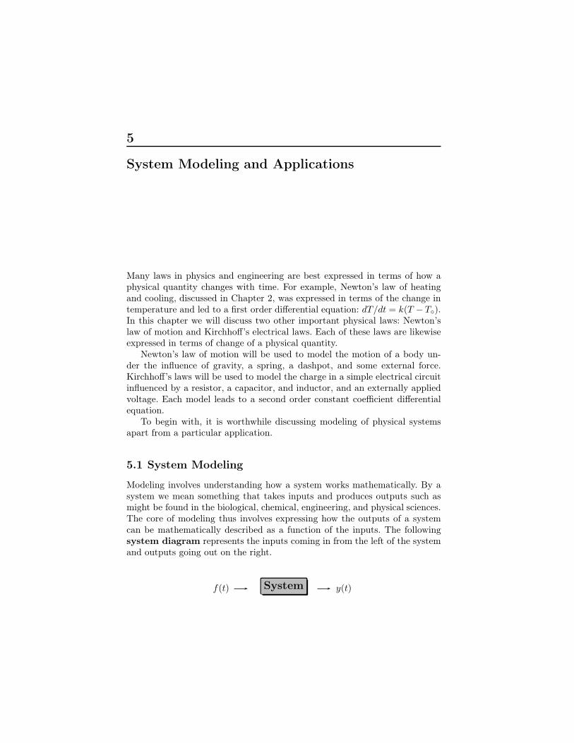
5
System Modeling and Applications
Many laws in physics and engineering are best expressed in terms of how aphysical quantity changes with time. For example, Newton’s law of heatingand cooling, discussed in Chapter 2, was expressed in terms of the change intemperature and led to a first order differential equation: dT/dt = k(T − T).In this chapter we will discuss two other important physical laws: Newton’slaw of motion and Kirchhoff’s electrical laws. Each of these laws are likewiseexpressed in terms of change of a physical quantity.
Newton’s law of motion will be used to model the motion of a body un-der the influence of gravity, a spring, a dashpot, and some external force.Kirchhoff’s laws will be used to model the charge in a simple electrical circuitinfluenced by a resistor, a capacitor, and inductor, and an externally appliedvoltage. Each model leads to a second order constant coefficient differentialequation.
To begin with, it is worthwhile discussing modeling of physical systemsapart from a particular application.
5.1 System Modeling
Modeling involves understanding how a system works mathematically. By asystem we mean something that takes inputs and produces outputs such asmight be found in the biological, chemical, engineering, and physical sciences.The core of modeling thus involves expressing how the outputs of a systemcan be mathematically described as a function of the inputs. The followingsystem diagram represents the inputs coming in from the left of the systemand outputs going out on the right.
f(t) System y(t)
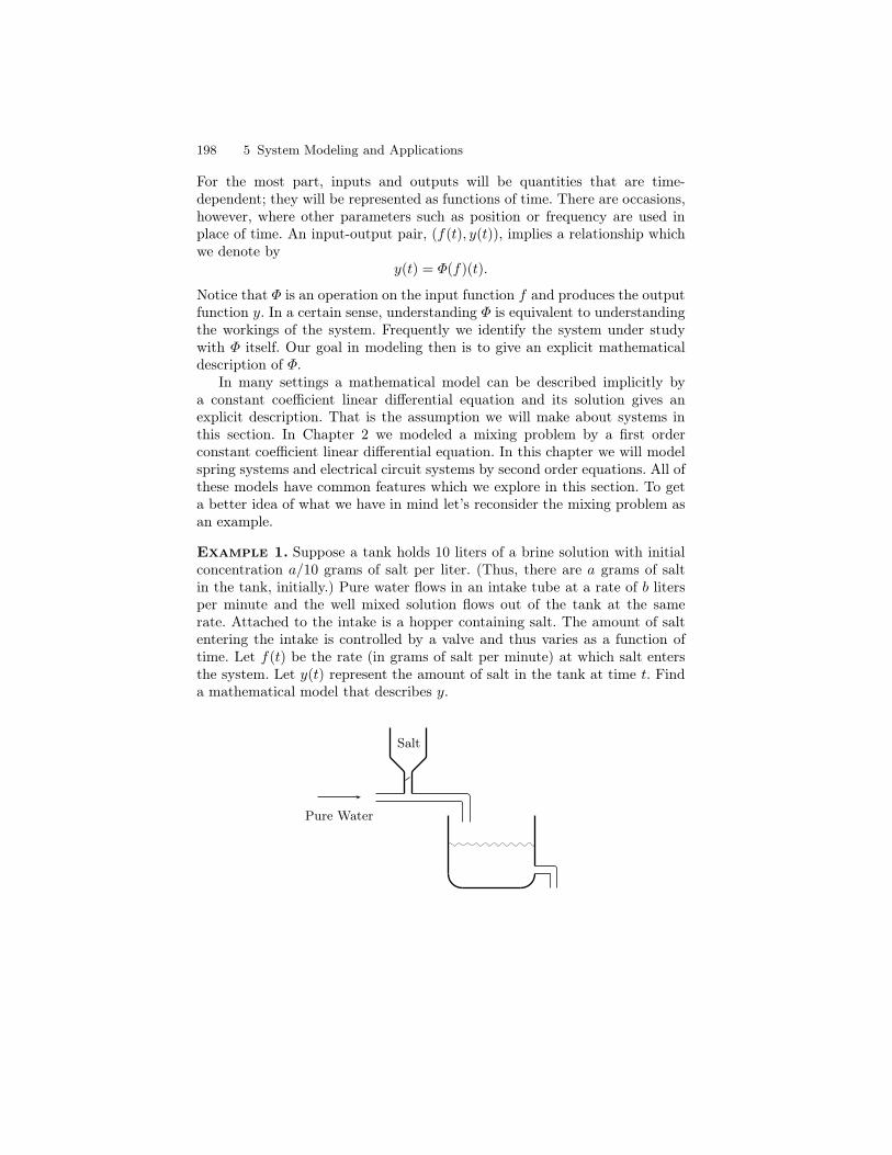
198 5 System Modeling and Applications
For the most part, inputs and outputs will be quantities that are time-dependent; they will be represented as functions of time. There are occasions,however, where other parameters such as position or frequency are used inplace of time. An input-output pair, (f(t), y(t)), implies a relationship whichwe denote by
y(t) = Φ(f)(t).
Notice that Φ is an operation on the input function f and produces the outputfunction y. In a certain sense, understanding Φ is equivalent to understandingthe workings of the system. Frequently we identify the system under studywith Φ itself. Our goal in modeling then is to give an explicit mathematicaldescription of Φ.
In many settings a mathematical model can be described implicitly bya constant coefficient linear differential equation and its solution gives anexplicit description. That is the assumption we will make about systems inthis section. In Chapter 2 we modeled a mixing problem by a first orderconstant coefficient linear differential equation. In this chapter we will modelspring systems and electrical circuit systems by second order equations. All ofthese models have common features which we explore in this section. To geta better idea of what we have in mind let’s reconsider the mixing problem asan example.
Example 1. Suppose a tank holds 10 liters of a brine solution with initialconcentration a/10 grams of salt per liter. (Thus, there are a grams of saltin the tank, initially.) Pure water flows in an intake tube at a rate of b litersper minute and the well mixed solution flows out of the tank at the samerate. Attached to the intake is a hopper containing salt. The amount of saltentering the intake is controlled by a valve and thus varies as a function oftime. Let f(t) be the rate (in grams of salt per minute) at which salt entersthe system. Let y(t) represent the amount of salt in the tank at time t. Finda mathematical model that describes y.
Salt
Pure Water
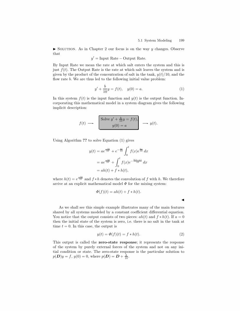
5.1 System Modeling 199
I Solution. As in Chapter 2 our focus is on the way y changes. Observethat
y′ = Input Rate−Output Rate.
By Input Rate we mean the rate at which salt enters the system and this isjust f(t). The Output Rate is the rate at which salt leaves the system and isgiven by the product of the concentration of salt in the tank, y(t)/10, and theflow rate b. We are thus led to the following initial value problem:
y′ +b
10y = f(t), y(0) = a. (1)
In this system f(t) is the input function and y(t) is the output function. In-corporating this mathematical model in a system diagram gives the followingimplicit description:
f(t)Solve y′ + b
10y = f(t),
y(0) = ay(t).
Using Algorithm ?? to solve Equation (1) gives
y(t) = ae−bt10 + e−
bt10
∫ t
0
f(x)ebx10 dx
= ae−bt10 +
∫ t
0
f(x)e−b(t−x)
10 dx
= ah(t) + f ∗ h(t),
where h(t) = e−bt10 and f ∗h denotes the convolution of f with h. We therefore
arrive at an explicit mathematical model Φ for the mixing system:
Φ(f)(t) = ah(t) + f ∗ h(t).
J
As we shall see this simple example illustrates many of the main featuresshared by all systems modeled by a constant coefficient differential equation.You notice that the output consists of two pieces: ah(t) and f ∗ h(t). If a = 0then the initial state of the system is zero, i.e. there is no salt in the tank attime t = 0. In this case, the output is
y(t) = Φ(f)(t) = f ∗ h(t). (2)
This output is called the zero-state response; it represents the responseof the system by purely external forces of the system and not on any ini-tial condition or state. The zero-state response is the particular solution top(D)y = f , y(0) = 0, where p(D) = D + b
10 .
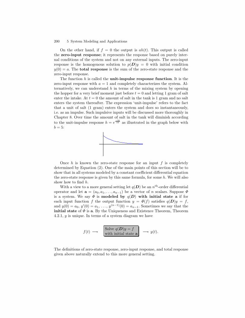
200 5 System Modeling and Applications
On the other hand, if f = 0 the output is ah(t). This output is calledthe zero-input response; it represents the response based on purely inter-nal conditions of the system and not on any external inputs. The zero-inputresponse is the homogenous solution to p(D)y = 0 with initial conditiony(0) = a. The total response is the sum of the zero-state response and thezero-input response.
The function h is called the unit-impulse response function. It is thezero-input response with a = 1 and completely characterizes the system. Al-ternatively, we can understand h in terms of the mixing system by openingthe hopper for a very brief moment just before t = 0 and letting 1 gram of saltenter the intake. At t = 0 the amount of salt in the tank is 1 gram and no saltenters the system thereafter. The expression ‘unit-impulse’ refers to the factthat a unit of salt (1 gram) enters the system and does so instantaneously,i.e. as an impulse. Such impulsive inputs will be discussed more thoroughly inChapter 8. Over time the amount of salt in the tank will diminish accordingto the unit-impulse response h = e
−bt10 as illustrated in the graph below with
b = 5:
Once h is known the zero-state response for an input f is completelydetermined by Equation (2). One of the main points of this section will be toshow that in all systems modeled by a constant coefficient differential equationthe zero-state response is given by this same formula, for some h. We will alsoshow how to find h.
With a view to a more general setting let q(D) be an nth-order differentialoperator and let a = (a0, a1, . . . , an−1) be a vector of n scalars. Suppose Φis a system. We say Φ is modeled by q(D) with initial state a if foreach input function f the output function y = Φ(f) satisfies q(D)y = f ,and y(0) = a0, y
′(0) = a1, . . . , y(n−1)(0) = an−1. Sometimes we say that the
initial state of Φ is a. By the Uniqueness and Existence Theorem, Theorem4.2.1, y is unique. In terms of a system diagram we have
f(t)Solve q(D)y = fwith initial state a
y(t).
The definitions of zero-state response, zero-input response, and total responsegiven above naturally extend to this more general setting.
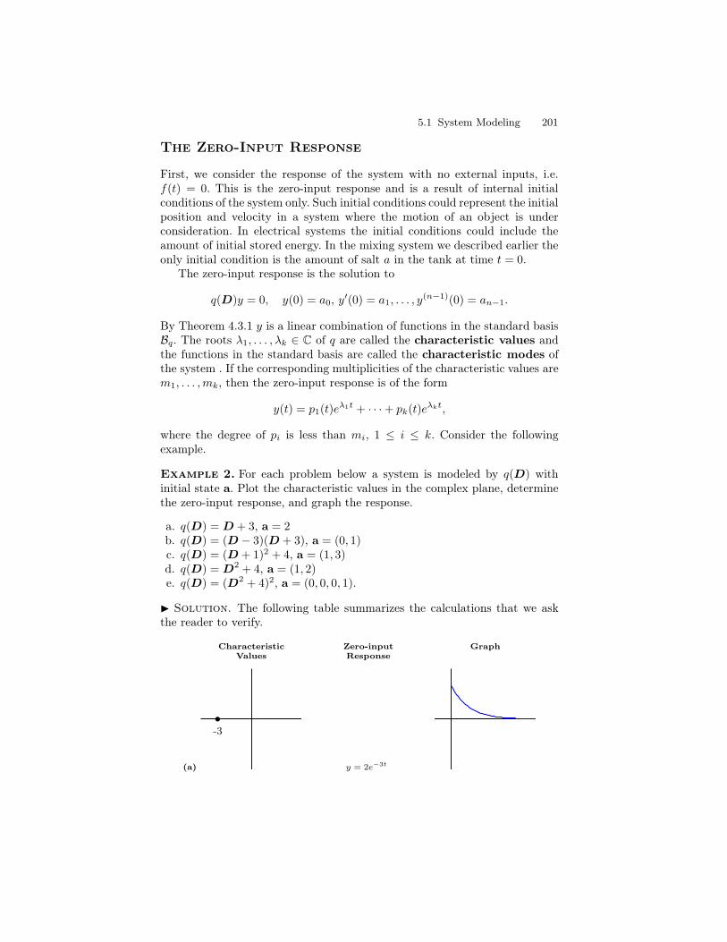
5.1 System Modeling 201
The Zero-Input Response
First, we consider the response of the system with no external inputs, i.e.f(t) = 0. This is the zero-input response and is a result of internal initialconditions of the system only. Such initial conditions could represent the initialposition and velocity in a system where the motion of an object is underconsideration. In electrical systems the initial conditions could include theamount of initial stored energy. In the mixing system we described earlier theonly initial condition is the amount of salt a in the tank at time t = 0.
The zero-input response is the solution to
q(D)y = 0, y(0) = a0, y′(0) = a1, . . . , y
(n−1)(0) = an−1.
By Theorem 4.3.1 y is a linear combination of functions in the standard basisBq. The roots λ1, . . . , λk ∈ C of q are called the characteristic values andthe functions in the standard basis are called the characteristic modes ofthe system . If the corresponding multiplicities of the characteristic values arem1, . . . ,mk, then the zero-input response is of the form
y(t) = p1(t)eλ1t + · · ·+ pk(t)eλkt,
where the degree of pi is less than mi, 1 ≤ i ≤ k. Consider the followingexample.
Example 2. For each problem below a system is modeled by q(D) withinitial state a. Plot the characteristic values in the complex plane, determinethe zero-input response, and graph the response.
a. q(D) = D + 3, a = 2b. q(D) = (D − 3)(D + 3), a = (0, 1)c. q(D) = (D + 1)2 + 4, a = (1, 3)d. q(D) = D2 + 4, a = (1, 2)e. q(D) = (D2 + 4)2, a = (0, 0, 0, 1).
I Solution. The following table summarizes the calculations that we askthe reader to verify.
Characteristic Zero-input GraphValues Response
(a)
-3
y = 2e−3t
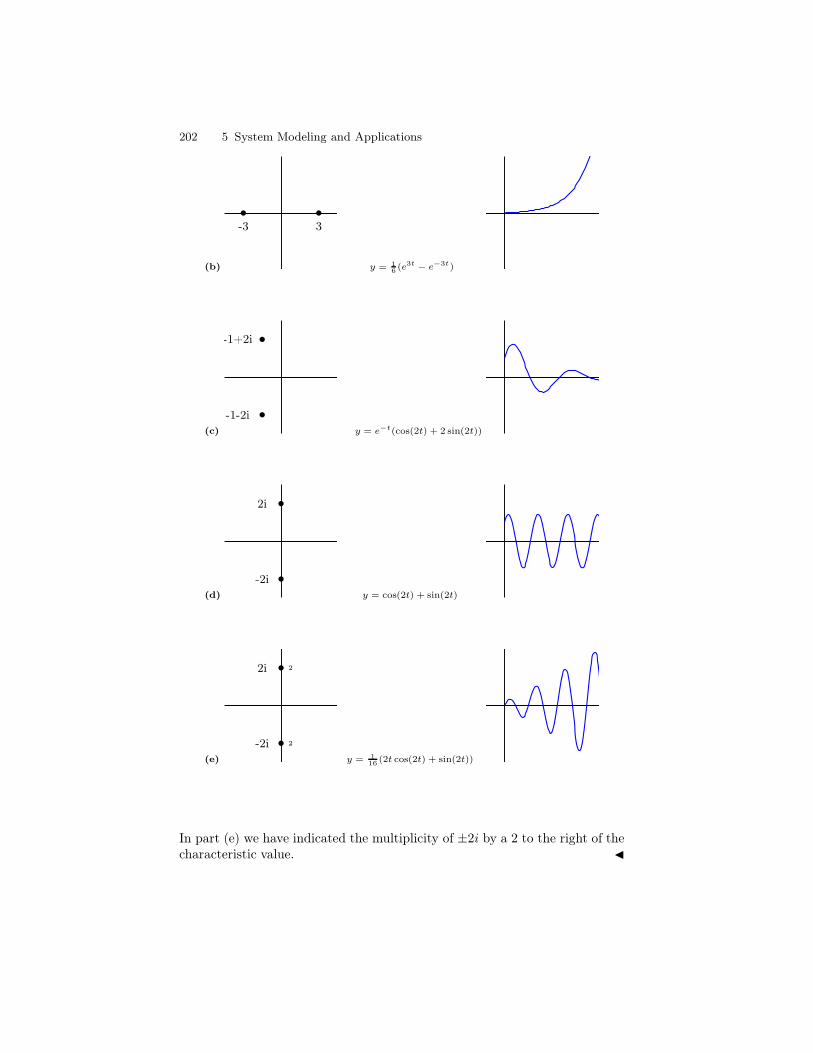
202 5 System Modeling and Applications
(b)
-3 3
y = 16 (e3t − e−3t)
(c)
-1+2i
-1-2iy = e−t(cos(2t) + 2 sin(2t))
(d)
2i
-2iy = cos(2t) + sin(2t)
(e)
2i
-2i
2
2
y = 116 (2t cos(2t) + sin(2t))
In part (e) we have indicated the multiplicity of ±2i by a 2 to the right of thecharacteristic value. J
5.1 System Modeling 203
The location of the characteristic values in the complex plane is related toan important notion called system stability.
stability
System stability has to do with the long term behavior of a system. If thezero-input response of a system, for all initial states, tends to zero over timethen we say the system is asymptotically stable. This behavior is seenin the mixing system of Example 1. For any initial state a the zero-inputresponse y(t) = ae
−bt10 has limiting value 0 as t → ∞. In the case a = 2 and
b = 30 the graph is the same as that given in Example 2a. Notice that thesystem in Example 2c is also asymptotically stable since zero-input responsealways takes the form y(t) = e−t(A sin(2t) + B cos(2t)). The function t →A sin(2t) + B cos(2t) is bounded, so the presence of e−t guarantees that thelimit value of y(t) is 0 as t→∞. In both Example 2a and 2c the characteristicvalues lie in the left-half side of the complex plane. More generally, supposetkeλt is a characteristic mode for a system. If λ = α+ iβ and α < 0 then
limt→∞
tkeλt = 0,
for all nonnegative integers k. On the other hand, if α > 0 then the charac-teristic mode, tkeλt is unbounded. Thus a system is asymptotically stable ifand only if all characteristic values lie to the left of the imaginary axis.
If a system is not asymptotically stable but the zero-input response isbounded for all possible initial states then we say the system is marginallystable. Marginal stability is seen in Example 2d and occurs when one or moreof the characteristic values lie on the imaginary axis and have multiplicityexactly one. Those characteristic values that are not on the imaginary axismust be to the left of the imaginary axis.
We say a system is unstable if there is an initial state in which the zero-input response is unbounded over time. This behavior can be seen in Example2b and 2e. Over time the response becomes unbounded. Of course, in a realphysical system this cannot happen. The system will break or explode whenit passes a certain threshold. Unstable systems occur for two distinct reasons.First, if one of the characteristic values is λ = α + iβ and α > 0 then λlies in the right-half side of the complex plane. In this case the characteristicmode is of the form tkeλt. This function is unbounded as a function of t. Thisis what happens in Example 2b. Second, if one of the characteristic valuesλ = iβ lies on the imaginary axis and, in addition, the multiplicity is greaterthan one then the characteristic mode is of the form tkeiβt, k ≥ 1. This modeoscillates unboundedly as a function of t > 0, as in Example 2e. Remember,it only takes one unbounded characteristic mode for the whole system to beunstable.
Example 3. Determine the stability of each system modeled by q(D) below.
204 5 System Modeling and Applications
1. q(D) = (D + 1)2(D + 3)2. q(D) = (D2 + 9)(D + 4)3. q(D) = (D + 4)2(D − 5)4. q(D) = (D2 + 1)(D2 + 9)2
I Solution.
1. The characteristic values are λ = −1 with multiplicity 2 and λ = −3. Thesystem is asymptotically stable.
2. The characteristic values are λ = ±3i and λ = −4. The system is mar-ginally stable.
3. The characteristic values are λ = −4 with multiplicity 2 and λ = 5. Thesystem is unstable.
4. The characteristic values are λ = ±i and λ = ±3i with multiplicity 2. Thesystem is unstable.
the unit-impulse response function
Suppose Φ is a system modeled by q(D), an nth order constant coefficientdifferential operator. The unit-impulse response function h(t) is the zero-input response to Φ when the initial state of the system is a = (0, . . . , 0, 1).More specifically, h(t) is the solution to
q(D)y = 0 y(0) = 0, . . . , y(n−2)(0) = 0, y(n−1)(0) = 1.
If n = 1 then y(0) = 1 as in the mixing system discussed in the beginningof this section. In this simple case h(t) is a multiple of a single characteristicmode. For higher order systems, however, the unit-impulse response functionis a homogeneous solution to q(D)y = 0 and, hence, a linear combination ofthe characteristic modes of the system.
Example 4. Find the unit-impulse response function for a system Φ mod-eled by
q(D) = (D + 1)(D2 + 1).
I Solution. It is an easy matter to apply the Laplace transform method toq(D)y = 0 with initial condition y(0) = 0, y′(0) − 0, and y′′(0) = 1. We getq(s)Y (s)− 1 = 0. A short calculation gives
Y (s) =1
q(s)=
1
(s+ 1)(s2 + 1)=
1
4
(
2
s+ 1+−2s+ 2
s2 + 1
)
.
The inverse Laplace transform is y(t) =1
2(e−t+sin t−cos t). The unit-impulse
response function is thus
h(t) =1
2(e−t + sin t− cos t).
5.1 System Modeling 205
J
Observe in this example that h(t) = L−1 1q(s)(t). It is not hard to see
that this formula extends to the general case. We record this in the followingtheorem. The proof is left to the reader.
Theorem 5. Suppose a system Φ is modeled by a constant coefficient differ-ential operator q(D). The unit-impulse response function, h(t), of the systemΦ is given by
h(t) = L−1
1
q(s)
(t).
The Zero-State Response
Let’s now turn our attention to a system Φ in the zero-state and consider thezero-state response. This occurs precisely when a = 0, ie. all initial conditionsof the system are zero. We should think of the system as initially being at rest.We continue to assume that Φ is modeled by an nth-order constant coefficientdifferential operator q(D). Thus, for each input f(t) the output y(t) satisfiesq(D)y = f with y and its higher derivatives up to order n−1 all zero at t = 0.An important feature of Φ in this case is its linearity.
Proposition 6. Suppose Φ is a system modeled by q(D) in the zero-state.Then Φ is linear. Specifically, if f , f1 and f2 are input functions and c is ascalar then
1. Φ(f1 + f2) = Φ(f1) + Φ(f2)2. Φ(cf) = cΦ(f)
Proof. If f is any input function then Φ(f) = y if and only if q(D)y = f andy(0) = y′(0) = · · · = y(n−1)(0) = 0. If y1 and y2 are the zero-state responsefunctions to f1 and f2, respectively, then the linearity of q(D) implies
q(D)(y1 + y2) = q(D)y1 + q(D)y2 = f1 + f2.
Furthermore, since the initial state of both y1 and y2 are zero so is the initialstate of y1 + y2. This implies Φ(f1 + f2) = y1 + y2. In a similar way,
q(D)(cy) = cq(D)y = cf,
by the linearity of q(D). The initial state of cy is clearly zero. So Φ(cf) =cΦ(f). utTheorem 7. Suppose Φ is a system modeled by q(D) in the zero-state. If f isa continuous input function on an interval which includes zero then the zero-state response is given by the convolution of f with the unit-impulse responsefunction h. I.e.
φ(f)(t) = f ∗ h(t) =
∫ t
0
f(x)h(t− x) dx.
206 5 System Modeling and Applications
Before we proceed with the proof let’s introduce the following helpfullemma.
Lemma 8. Suppose f is continuous on a interval I containing 0. Suppose his differentiable on I. Then
(f ∗ h)′(t) = f(t)h(0) + f ∗ h′.
Proof. Let y(t) = f ∗ h(t). Then
∆y
∆t=y(t+∆t)− y(t)
∆t
=1
∆t
(
∫ t+∆t
0
f(x)h(t +∆t− x) dx −∫ t
0
f(x)h(t− x) dx)
=
∫ t
0
f(x)h(t+∆t− x)− h(t− x)
∆tdx +
1
∆t
∫ t+∆t
t
f(x)h(t+∆t− x) dx.
We now let ∆t go to 0. The first summand has limit∫ t
0f(x)h′(t − x) dx =
f ∗ h′(t). By the Fundamental Theorem of Calculus the limit of the secondsummand is obtained by evaluating the integrand at x = t, thus gettingf(t)h(0). The lemma now follows by adding these two terms. ut
Proof (of Theorem 7). Let h(t) be the unit-impulse response function. Thenh(0) = h′(0) = · · · = h(n−2)(0) = 0 and h(n−1)(0) = 1. Set y(t) = f ∗ h(t).Repeated applications of Lemma 8 to y gives
y′ = f ∗ h′ + h(0)f = f ∗ hy′′ = f ∗ h′′ + h′(0)f = f ∗ h′′
...
y(n−1) = f ∗ h(n−1) + h(n−2)(0)f = f ∗ h(n−1)
y(n) = f ∗ h(n) + h(n−1)(0)f = f ∗ h(n) + f.
From this it follows that
q(D)y = f ∗ q(D)h+ f = f,
since q(D)h = 0. It is easy to check that y is in the zero-state. Therefore
Φ(f) = y = f ∗ h.
ut
5.1 System Modeling 207
At this point let us make a few remarks on what this theorem tells us. Themost remarkable thing is the fact that Φ is precisely determined by the unit-impulse response function h. From a mathematical point of view, knowing hmeans you know how the system Φ works in the zero-state. Once h is deter-mined all output functions, i.e. system responses, are given by the convolutionproduct, f ∗h, for an input function f . Admittedly, convolution is an unusualproduct. It is not at all like the usual product of functions where the value (orstate) at time t is determined by knowing just the value of each factor at timet. Theorem 7 tells us that the state of a system response at time t dependson knowing the values of the input function f for all x between 0 and t. Thesystem ‘remembers’ the whole of the input f up to time t and ‘meshes’ thoseinputs with the internal workings of the system, as represented by impulseresponse function h, to give f ∗ h(t).
Since the zero-state response, f ∗ h, is a solution to q(D)y = f , with zeroinitial state, it is a particular solution. This formula thus gives an alternativeto the method of undetermined coefficients and the incomplete partial fractionmethod. We can also take the opposite view. The method of undeterminedcoefficients and the incomplete partial fraction method are alternative waysto compute a convolution f ∗h, when f and h are in E . In practice, computingconvolutions can be time consuming and tedious. In the following exampleswe will limit the inputs to functions in EC and use Table ??.
Example 9. A system Φ is modeled by q(D). Find the zero-state responsefor the given input function.
a) q(D) = D + 2 and f(t) = 1b) q(D) = D2 + 4D + 3 and f(t) = e−t
c) q(D) = D2 + 4 and f(t) = cos(2t)
I Solution.
a) The characteristic polynomial is q(s) = s+ 2 and therefore the character-istic mode is e−2t. It follows that h(t) = Ae−2t and with initial conditionh(0) = 1 we get h(t) = e−2t. The system response, y(t), for the input 1 is
y(t) = e−2t ∗ 1(t) =1
2(1− e−2t).
b) The characteristic polynomial is q(s) = s2 + 4s+ 3 = (s+ 1)(s+ 3). Thecharacteristic modes are e−3t and e−t. Thus h(t) has the form h(t) =Ae−t +Be−3t. The initial conditions h(0) = 0 and h′(0) = 1 implies
h(t) =1
2(e−t − e−3t).
The system response to the input function f(t) = e−t is
y(t) =1
2(e−t − e−3t) ∗ e−t =
1
2te−t − 1
4e−t +
1
4e−3t.
208 5 System Modeling and Applications
c) It is easy to verify that the impulse response function is h(t) = 12 sin(2t).
The system response to the input function f(t) = cos(2t) is
y(t) =1
2sin(2t) ∗ cos(2t) =
1
4t sin(2t).
J
bounded-in bounded-out
In Example 9a we introduce a bounded input, f(t) = 1, and the responsey(t) = 1
2 (1 − e−2t) is also bounded, by 12 , in fact. On the other hand, in
Example 9c, we introduce a bounded input, f(t) = cos 2t, yet the responsey(t) = 1
4 t sin 2t oscillates unboundedly. We say that a system Φ is BIBO-stable if for every bounded input f(t) the response function y(t) is likewisebounded. (BIBO stands for ‘bounded input bounded output’.) Note the fol-lowing theorem. An outline of the proof is given in the exercises.
Theorem 10. Suppose Φ is an asymptotically stable system. Then Φ is BIBO-stable.
Unstable systems are of little practical value to an engineer designing a‘safe’ system. In an unstable system a set of unintended initial states can leadto an unbounded response that destroys the system entirely. Even marginallystable systems can have bounded input functions that produce unboundedoutput functions. This is seen in Example 9c, where the system response tothe bounded input f(t) = cos(2t) is the unbounded function y(t) = 1
4 t sin(2t).Asymptotically stable systems are thus the ‘safest’ systems since they areBIBO-stable. They produce at worst a bounded response to a bounded input.However, this is not to say that the response can not be destructive. We willsay more about this in the following topic.
resonance
We now come to a very interesting and important phenomenon called res-onance. Loosely speaking, resonance is the phenomenon that occurs whena system reacts very energetically to a relatively mild input. Resonance cansometimes be catastrophic for the system. For example, a wine glass has anatural frequency at which it will vibrate. You can hear this frequency byrubbing your moistened finger around the rim of the glass to cause it to vi-brate. An opera singer who sings a note at this same frequency with sufficientintensity can cause the wine glass to vibrate so much that it shatters. Reso-nance can also be used to our advantage as is familiar to a musician tuning amusical instrument to a standard frequency given, for example, by a tuningfork. Resonance occurs when the instrument is ‘in tune’.
The characteristic values of a system Φ are sometimes referred to as thecharacteristic frequencies. As we saw earlier the internal workings of a
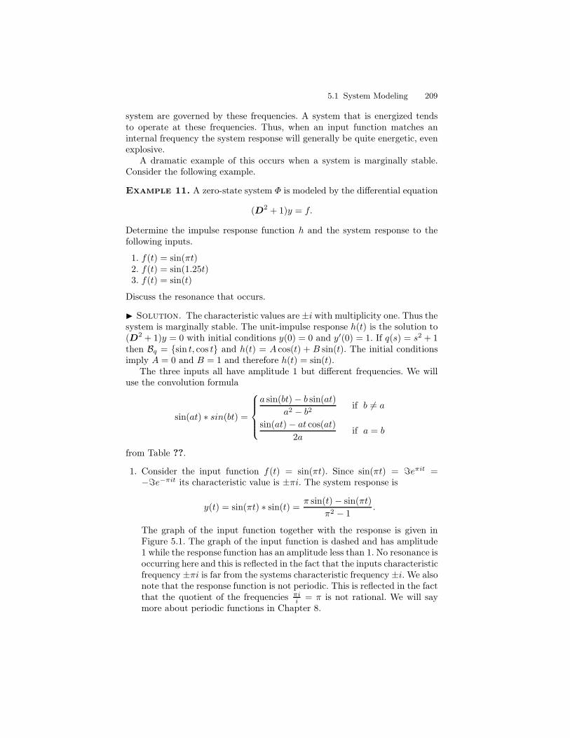
5.1 System Modeling 209
system are governed by these frequencies. A system that is energized tendsto operate at these frequencies. Thus, when an input function matches aninternal frequency the system response will generally be quite energetic, evenexplosive.
A dramatic example of this occurs when a system is marginally stable.Consider the following example.
Example 11. A zero-state system Φ is modeled by the differential equation
(D2 + 1)y = f.
Determine the impulse response function h and the system response to thefollowing inputs.
1. f(t) = sin(πt)2. f(t) = sin(1.25t)3. f(t) = sin(t)
Discuss the resonance that occurs.
I Solution. The characteristic values are±i with multiplicity one. Thus thesystem is marginally stable. The unit-impulse response h(t) is the solution to(D2 + 1)y = 0 with initial conditions y(0) = 0 and y′(0) = 1. If q(s) = s2 + 1then Bq = sin t, cos t and h(t) = A cos(t) + B sin(t). The initial conditionsimply A = 0 and B = 1 and therefore h(t) = sin(t).
The three inputs all have amplitude 1 but different frequencies. We willuse the convolution formula
sin(at) ∗ sin(bt) =
a sin(bt)− b sin(at)
a2 − b2 if b 6= a
sin(at)− at cos(at)
2aif a = b
from Table ??.
1. Consider the input function f(t) = sin(πt). Since sin(πt) = =eπit =−=e−πit its characteristic value is ±πi. The system response is
y(t) = sin(πt) ∗ sin(t) =π sin(t)− sin(πt)
π2 − 1.
The graph of the input function together with the response is given inFigure 5.1. The graph of the input function is dashed and has amplitude1 while the response function has an amplitude less than 1. No resonance isoccurring here and this is reflected in the fact that the inputs characteristicfrequency ±πi is far from the systems characteristic frequency ±i. We alsonote that the response function is not periodic. This is reflected in the factthat the quotient of the frequencies πi
i = π is not rational. We will saymore about periodic functions in Chapter 8.
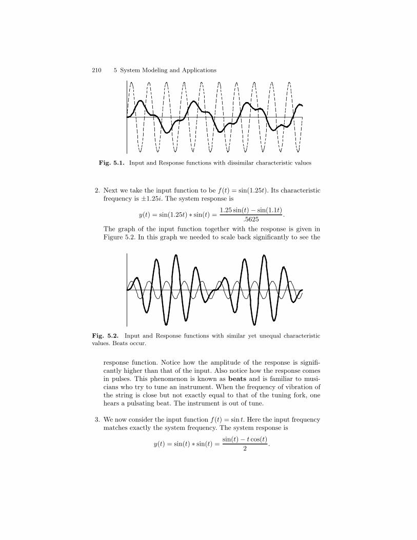
210 5 System Modeling and Applications
Fig. 5.1. Input and Response functions with dissimilar characteristic values
2. Next we take the input function to be f(t) = sin(1.25t). Its characteristicfrequency is ±1.25i. The system response is
y(t) = sin(1.25t) ∗ sin(t) =1.25 sin(t)− sin(1.1t)
.5625.
The graph of the input function together with the response is given inFigure 5.2. In this graph we needed to scale back significantly to see the
Fig. 5.2. Input and Response functions with similar yet unequal characteristicvalues. Beats occur.
response function. Notice how the amplitude of the response is signifi-cantly higher than that of the input. Also notice how the response comesin pulses. This phenomenon is known as beats and is familiar to musi-cians who try to tune an instrument. When the frequency of vibration ofthe string is close but not exactly equal to that of the tuning fork, onehears a pulsating beat. The instrument is out of tune.
3. We now consider the input function f(t) = sin t. Here the input frequencymatches exactly the system frequency. The system response is
y(t) = sin(t) ∗ sin(t) =sin(t)− t cos(t)
2.
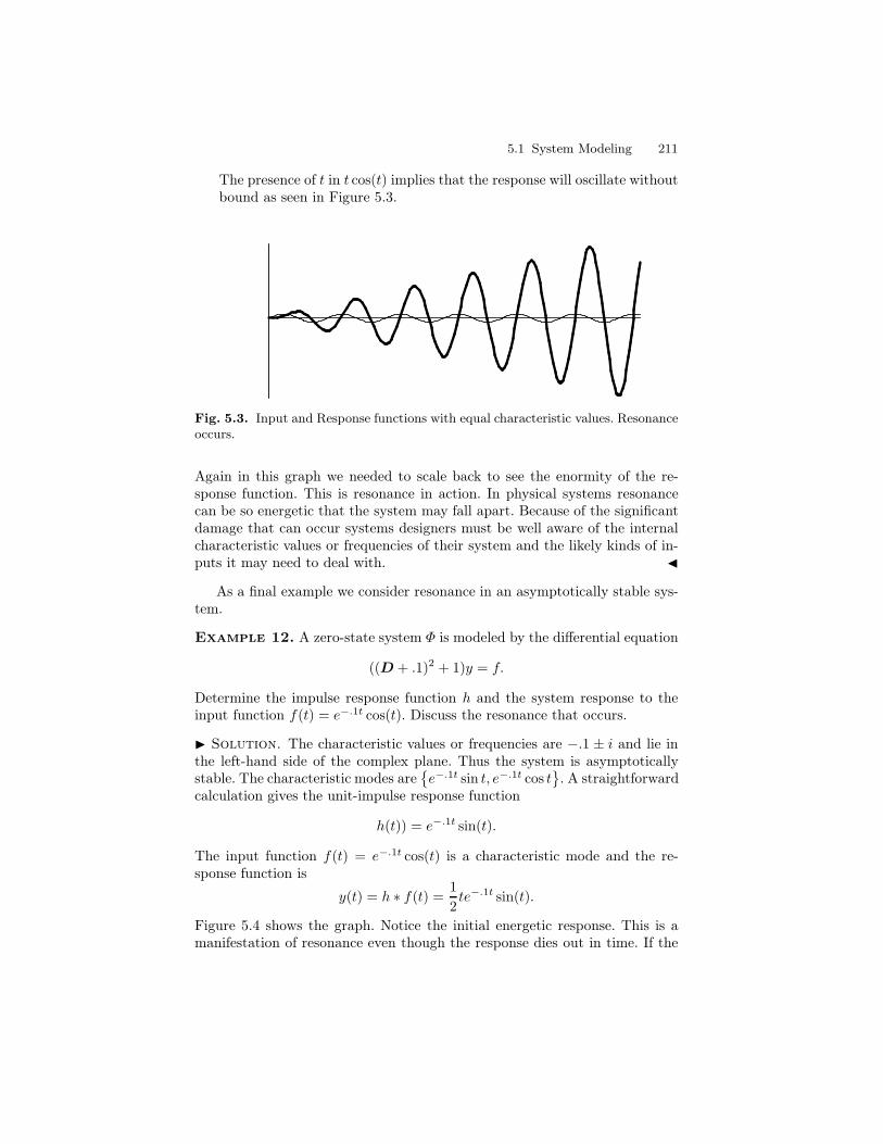
5.1 System Modeling 211
The presence of t in t cos(t) implies that the response will oscillate withoutbound as seen in Figure 5.3.
Fig. 5.3. Input and Response functions with equal characteristic values. Resonanceoccurs.
Again in this graph we needed to scale back to see the enormity of the re-sponse function. This is resonance in action. In physical systems resonancecan be so energetic that the system may fall apart. Because of the significantdamage that can occur systems designers must be well aware of the internalcharacteristic values or frequencies of their system and the likely kinds of in-puts it may need to deal with. J
As a final example we consider resonance in an asymptotically stable sys-tem.
Example 12. A zero-state system Φ is modeled by the differential equation
((D + .1)2 + 1)y = f.
Determine the impulse response function h and the system response to theinput function f(t) = e−.1t cos(t). Discuss the resonance that occurs.
I Solution. The characteristic values or frequencies are −.1 ± i and lie inthe left-hand side of the complex plane. Thus the system is asymptoticallystable. The characteristic modes are
e−.1t sin t, e−.1t cos t
. A straightforwardcalculation gives the unit-impulse response function
h(t)) = e−.1t sin(t).
The input function f(t) = e−.1t cos(t) is a characteristic mode and the re-sponse function is
y(t) = h ∗ f(t) =1
2te−.1t sin(t).
Figure 5.4 shows the graph. Notice the initial energetic response. This is amanifestation of resonance even though the response dies out in time. If the
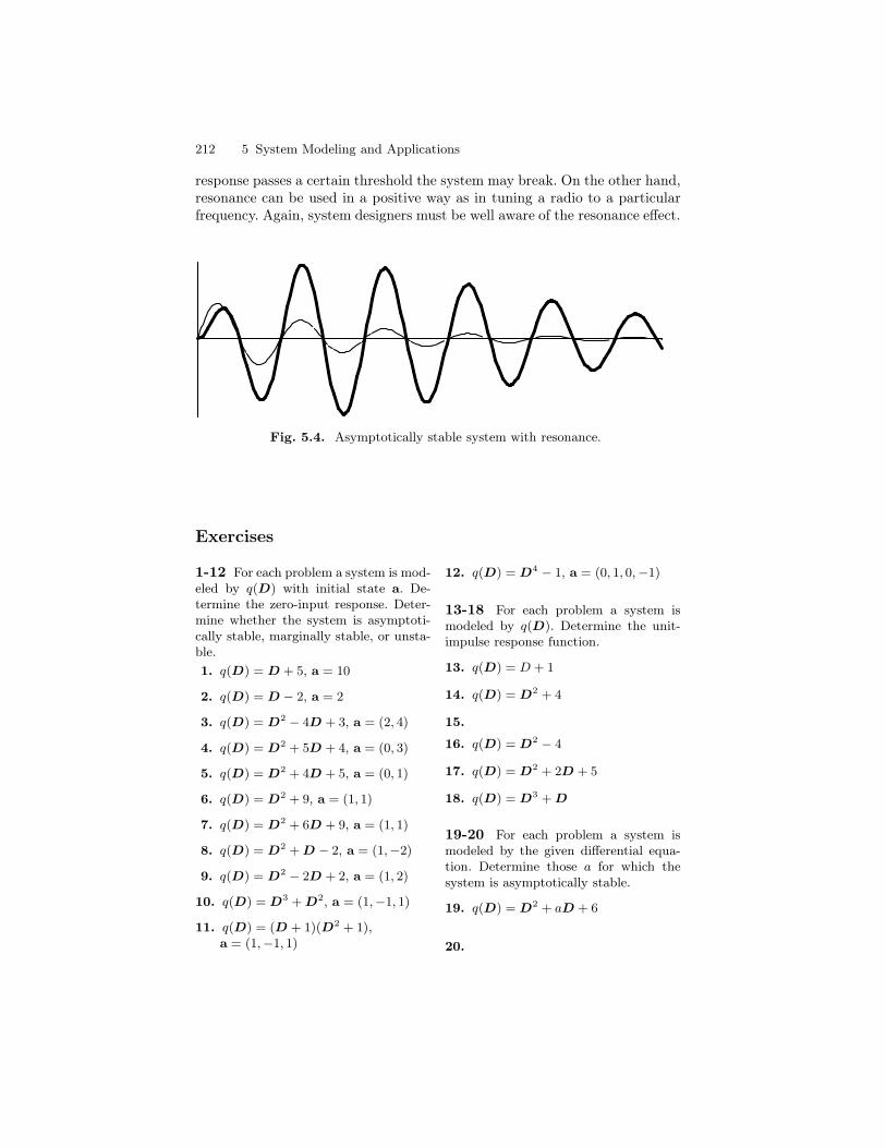
212 5 System Modeling and Applications
response passes a certain threshold the system may break. On the other hand,resonance can be used in a positive way as in tuning a radio to a particularfrequency. Again, system designers must be well aware of the resonance effect.
Fig. 5.4. Asymptotically stable system with resonance.
Exercises
1-12 For each problem a system is mod-eled by q(D) with initial state a. De-termine the zero-input response. Deter-mine whether the system is asymptoti-cally stable, marginally stable, or unsta-ble.
1. q(D) = D + 5, a = 10
2. q(D) = D − 2, a = 2
3. q(D) = D2 − 4D + 3, a = (2, 4)
4. q(D) = D2 + 5D + 4, a = (0, 3)
5. q(D) = D2 + 4D + 5, a = (0, 1)
6. q(D) = D2 + 9, a = (1, 1)
7. q(D) = D2 + 6D + 9, a = (1, 1)
8. q(D) = D2 +D − 2, a = (1,−2)
9. q(D) = D2 − 2D + 2, a = (1, 2)
10. q(D) = D3 +D2, a = (1,−1, 1)
11. q(D) = (D + 1)(D2 + 1),a = (1,−1, 1)
12. q(D) = D4 − 1, a = (0, 1, 0,−1)
13-18 For each problem a system ismodeled by q(D). Determine the unit-impulse response function.
13. q(D) = D + 1
14. q(D) = D2 + 4
15.
16. q(D) = D2 − 4
17. q(D) = D2 + 2D + 5
18. q(D) = D3 +D
19-20 For each problem a system ismodeled by the given differential equa-tion. Determine those a for which thesystem is asymptotically stable.
19. q(D) = D2 + aD + 6
20.
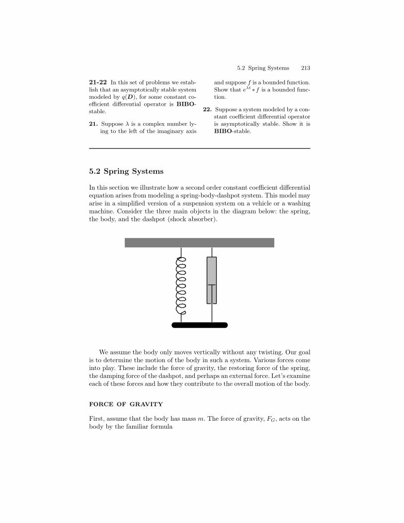
5.2 Spring Systems 213
21-22 In this set of problems we estab-lish that an asymptotically stable systemmodeled by q(D), for some constant co-efficient differential operator is BIBO-stable.
21. Suppose λ is a complex number ly-ing to the left of the imaginary axis
and suppose f is a bounded function.Show that eλt ∗ f is a bounded func-tion.
22. Suppose a system modeled by a con-stant coefficient differential operatoris asymptotically stable. Show it isBIBO-stable.
5.2 Spring Systems
In this section we illustrate how a second order constant coefficient differentialequation arises from modeling a spring-body-dashpot system. This model mayarise in a simplified version of a suspension system on a vehicle or a washingmachine. Consider the three main objects in the diagram below: the spring,the body, and the dashpot (shock absorber).
We assume the body only moves vertically without any twisting. Our goalis to determine the motion of the body in such a system. Various forces comeinto play. These include the force of gravity, the restoring force of the spring,the damping force of the dashpot, and perhaps an external force. Let’s examineeach of these forces and how they contribute to the overall motion of the body.
force of gravity
First, assume that the body has mass m. The force of gravity, FG, acts on thebody by the familiar formula
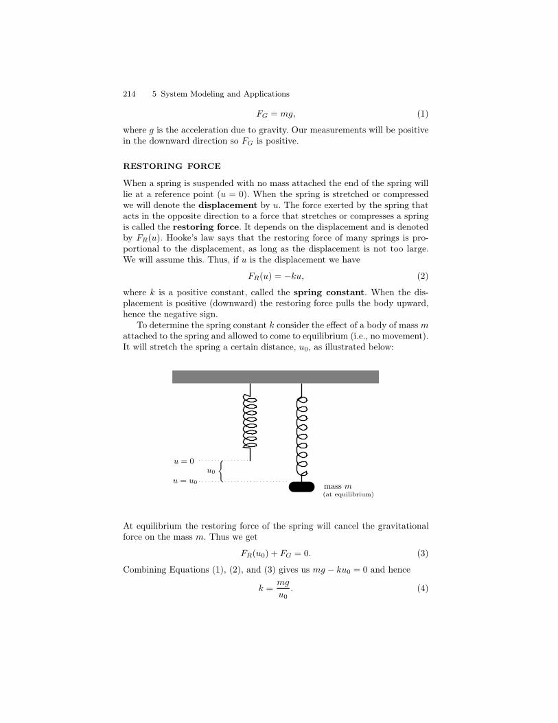
214 5 System Modeling and Applications
FG = mg, (1)
where g is the acceleration due to gravity. Our measurements will be positivein the downward direction so FG is positive.
restoring force
When a spring is suspended with no mass attached the end of the spring willlie at a reference point (u = 0). When the spring is stretched or compressedwe will denote the displacement by u. The force exerted by the spring thatacts in the opposite direction to a force that stretches or compresses a springis called the restoring force. It depends on the displacement and is denotedby FR(u). Hooke’s law says that the restoring force of many springs is pro-portional to the displacement, as long as the displacement is not too large.We will assume this. Thus, if u is the displacement we have
FR(u) = −ku, (2)
where k is a positive constant, called the spring constant. When the dis-placement is positive (downward) the restoring force pulls the body upward,hence the negative sign.
To determine the spring constant k consider the effect of a body of mass mattached to the spring and allowed to come to equilibrium (i.e., no movement).It will stretch the spring a certain distance, u0, as illustrated below:
u0
u = 0
u = u0mass m(at equilibrium)
At equilibrium the restoring force of the spring will cancel the gravitationalforce on the mass m. Thus we get
FR(u0) + FG = 0. (3)
Combining Equations (1), (2), and (3) gives us mg − ku0 = 0 and hence
k =mg
u0. (4)
5.2 Spring Systems 215
damping force
In any practical situation there will be some kind of resistance to the motionof the body. If our spring-body-dashpot system were under water the viscosityof the water would dampen the motion (no pun intended) to a much greaterextent than in air. In our system this resistance is represented by a dashpot,which in many situations is a shock absorber. The force exerted by the dashpotis called the damping force, FD. It depends on a lot of factors but animportant factor is the velocity of the body. To see that this is reasonableimagine the difference in the forces against your body when you dive intoa swimming pool off a 3 meter board and when you dive from the side ofthe pool. The greater the velocity when you enter the pool the greater theforce that decelerates your body. We will assume that the damping force isproportional to the velocity. We thus have
FD = −µv = −µu′,
where v = u′ is velocity and µ is a positive constant known as the dampingconstant. The damping force acts in a direction opposite the velocity, hencethe negative sign.
external forces and newton’s law of motion
We will let f(t) denote an external force acting on the body. For example, thiscould be the varying forces acting on a suspension system due to driving overa bumpy road. If a = u′′ is acceleration then Newton’s second law of motionsays that the total force of a body, given by mass times acceleration, is thesum of the forces acting on that body. We thus have
Total Force = FG + FR + FD + External Force,
which implies the equation
mu′′ = mg − ku− µu′ + f(t).
Equation 4 implies mg = −ku0. Substituting and combining terms gives
mu′′ + µu′ + k(u− u0) = f(t).
If y = u− u0 then y measures the displacement of the body from the equilib-rium point, u0. In this new variable we obtain
my′′ + µy′ + ky = f(t). (5)
This second order constant coefficient differential equation is a mathemat-ical model for the spring-body-dashpot system. The solutions that can be
216 5 System Modeling and Applications
obtained vary dramatically depending on the constants m, µ, and k, and, ofcourse, the external force, f(t). The initial conditions,
y(0) = y0 and y′(0) = v0
represent the initial position, y(0) = y0, and the initial velocity, y′(0) = v0 ofthe given body. Once the constants, external force, and initial conditions aredetermined the Uniqueness and Existence Theorem, Theorem 1, guaranteesa unique solution. Of course, we should always keep in mind that Equation 5is a mathematical model of a real phenomenon and its solution is an approx-imation to what really happens. However, as long as our assumptions aboutthe spring and damping constants are in effect, which usually require thaty(t) and y′(t) be relatively small in magnitude, and the mass of the spring isnegligible compared to the mass of the body, the solution will be a reasonablygood approximation.
units of measurement
Before we consider specific examples we summarize the two commonly usedunits of measurement: The English and Metric systems. The following tablesummarizes the units.
System Time Distance Mass Force
Metric seconds (s) meters (m) kilograms (kg) Newtons (N)English seconds (s) feet (ft) slugs (sl) pounds (lbs)
The main units of the English system are kilograms and meters while inthe English system they are pounds and feet. The time unit is common toboth. The next table summarizes quantities derived from these units.
Quantity Formula
velocity (v) distance / timeacceleration (a) velocity /timeforce (F) mass · accelerationspring constant (k) force / distancedamping constant (µ) force /velocity
In the metric system one Newton of force (N) will accelerate a one kilo-gram mass (kg) one m/s2. In the English system a one pound force (lb) willaccelerate a one slug mass (sl) one ft/s2. To compute the mass of a body in theEnglish system one must divide the weight by the acceleration due to gravity,which is g = 32 ft/sec2 near the surface of the earth. Thus a body weighing 64lbs has a mass of 2 slugs. To compute the force a body exerts due to gravity
5.2 Spring Systems 217
in the metric system one must multiply the mass by the acceleration due togravity, which is g = 9.8 m/sec2. Thus a 5 kg mass exerts a gravitational forceof 49 N.
Example 1.1. A body exerts a damping force of 10 pounds when the velocity of the mass
is 2 feet per second. Find the damping constant.2. A body exerts a damping force of 6 Newtons when the velocity is 40
centimeters per second. Find the damping constant3. A body weighing 4 pounds stretches a spring 2 inches. Find the spring
constant4. A mass of 8 kilograms stretches a spring 20 centimeters. Find the spring
constant.
I Solution.
1. The force is 10 pounds and the velocity is 2 feet per second. The dampingconstant is given by µ = Force/Velocity = 10/2 = 5.
2. The force is 6 Newtons and the velocity is .4 meters per second Thedamping constant is given by µ = Force/Velocity = 6/.4 = 15.
3. The force is 4 pounds. A length of 2 inches is 1/6 foot. The spring constantis k = Force/Distance = 4/(1/6) = 24.
4. The force exerted by a mass of 8 kilograms is 8 · 9.8 = 78.4 Newtons.A length of 20 centimeters is .2 meters. The spring constant is given byk = Force/Distance = 78.4/.2 = 392.
Example 2. A spring is stretched 20 centimeters by a force of 5 Newtons. Abody of mass 4 kilogram is attached to such a spring with an accompanyingdashpot. At t = 0 the mass is pulled down from its equilibrium position adistance of 50 centimeters and released with a downward velocity of 1 meterper second. Suppose the damping force is 5 Newtons when the velocity of thebody is .5 meter per second. Find a mathematical model that represents themotion of the body.
I Solution. We will model the motion by Equation 5. Units are convertedto the kilogram-meter units of the metric system. The mass is m = 4. Thespring constant k is given by k = 5/(.2) = 25. The damping constant is givenby µ = 5/.5 = 10. Since no external force is mentioned we may assume itis zero. The initial conditions are y(0) = .5 and y′(0) = 1. The followingequation
4y′′(t) + 10y′(t) + 25y = 0, y(0) = .5, y′(0) = 1
represents the model for the motion of the body. J
Example 3. A body weighing 4 pounds will stretch a spring 3 inches. Thissame body is attached to such a spring with an accompanying dashpot. Att = 0 the mass is pulled down from its equilibrium position a distance of 1
218 5 System Modeling and Applications
foot and released. Suppose the damping force is 8 pounds when the velocityof the body is 2 feet per second. Find a mathematical model that representsthe motion of the body.
I Solution. Units are converted to the pound-foot units in the Englishsystem. The mass is m = 4/32 = 1/8 slugs. The spring constant k is given byk = 4/(3/12) = 16. The damping constant is given by µ = 8/2 = 4. Since noexternal force is mentioned we may assume it is zero. The initial conditionsare y(0) = 1 and y′(0) = 0. The following equation
1
8y′′(t) + 4y′(t) + 16y = 0, y(0) = 1, y′(0) = 0
models the motion of the body. J
Let’s now turn our attention to an analysis of Equation (5). The zero-inputresponse models the motion of the body with no external forces. We refer tothis motion as free motion (f(t) ≡ 0). Otherwise we refer to the motion asforced motion (f(t) 6= 0). In turn each of these are divided into undamped(µ = 0) and damped (µ 6= 0).
Undamped Free Motion
When the damping constant is zero and there is no externally applied forcethe resulting motion of the object is called undamped free motion. This isan idealized situation, for seldom if ever will a system be free of any dampingeffects. Nevertheless, Equation (5) becomes
my′′ + ky = 0, (6)
with m > 0 and k > 0. The characteristic polynomial of this equation isq(s) = ms2 + k. Its characteristic values are ±iβ where β =
√
k/m, and itscharacteristic modes are sinβt, cosβt. Hence Equation (14) has the generalsolution
y = c1 cosβt+ c2 sinβt. (7)
Such is system is marginally stable as the characteristic values are purely com-plex. Using the trigonometric identity cos(βt−δ) = cos(βt) cos δ+sin(βt) sin δ,Equation (7) can be rewritten as
y = A cos(βt− δ) (8)
where c1 = A cos δ and c2 = A sin δ. Solving these equations for A and δgives A =
√
c21 + c22 and tan δ = c2/c1. Therefore, the graph of y(t) satisfyingEquation (14) is a pure cosine function with frequency β and with period
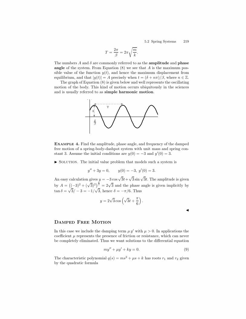
5.2 Spring Systems 219
T =2π
β= 2π
√
m
k.
The numbers A and δ are commonly referred to as the amplitude and phaseangle of the system. From Equation (8) we see that A is the maximum pos-sible value of the function y(t), and hence the maximum displacement fromequilibrium, and that |y(t)| = A precisely when t = (δ + nπ)/β, where n ∈ Z.
The graph of Equation (8) is given below and well represents the oscillatingmotion of the body. This kind of motion occurs ubiquitously in the sciencesand is usually referred to as simple harmonic motion.
A
y(t)
T
δβ
Example 4. Find the amplitude, phase angle, and frequency of the dampedfree motion of a spring-body-dashpot system with unit mass and spring con-stant 3. Assume the initial conditions are y(0) = −3 and y′(0) = 3.
I Solution. The initial value problem that models such a system is
y′′ + 3y = 0, y(0) = −3, y′(0) = 3.
An easy calculation gives y = −3 cos√
3t+√
3 sin√
3t. The amplitude is given
by A =(
(−3)2 + (√
3)2)
12 = 2
√3 and the phase angle is given implicitly by
tan δ =√
3/− 3 = −1/√
3, hence δ = −π/6. Thus
y = 2√
3 cos(√
3t+π
6
)
.
J
Damped Free Motion
In this case we include the damping term µ y′ with µ > 0. In applications thecoefficient µ represents the presence of friction or resistance, which can neverbe completely eliminated. Thus we want solutions to the differential equation
my′′ + µy′ + ky = 0. (9)
The characteristic polynomial q(s) = ms2 + µs+ k has roots r1 and r2 givenby the quadratic formula
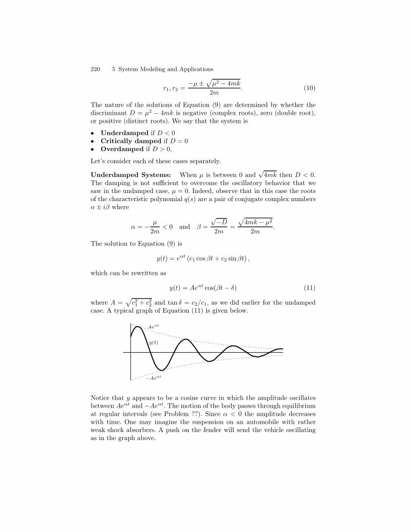
220 5 System Modeling and Applications
r1, r2 =−µ±
√
µ2 − 4mk
2m. (10)
The nature of the solutions of Equation (9) are determined by whether thediscriminant D = µ2 − 4mk is negative (complex roots), zero (double root),or positive (distinct roots). We say that the system is
• Underdamped if D < 0• Critically damped if D = 0• Overdamped if D > 0.
Let’s consider each of these cases separately.
Underdamped Systems: When µ is between 0 and√
4mk then D < 0.The damping is not sufficient to overcome the oscillatory behavior that wesaw in the undamped case, µ = 0. Indeed, observe that in this case the rootsof the characteristic polynomial q(s) are a pair of conjugate complex numbersα± iβ where
α = − µ
2m< 0 and β =
√−D2m
=
√
4mk − µ2
2m.
The solution to Equation (9) is
y(t) = eαt (c1 cosβt+ c2 sinβt) ,
which can be rewritten as
y(t) = Aeαt cos(βt− δ) (11)
where A =√
c21 + c22 and tan δ = c2/c1, as we did earlier for the undampedcase. A typical graph of Equation (11) is given below.
y(t)
Aeαt
−Aeαt
Notice that y appears to be a cosine curve in which the amplitude oscillatesbetween Aeαt and −Aeαt. The motion of the body passes through equilibriumat regular intervals (see Problem ??). Since α < 0 the amplitude decreaseswith time. One may imagine the suspension on an automobile with ratherweak shock absorbers. A push on the fender will send the vehicle oscillatingas in the graph above.
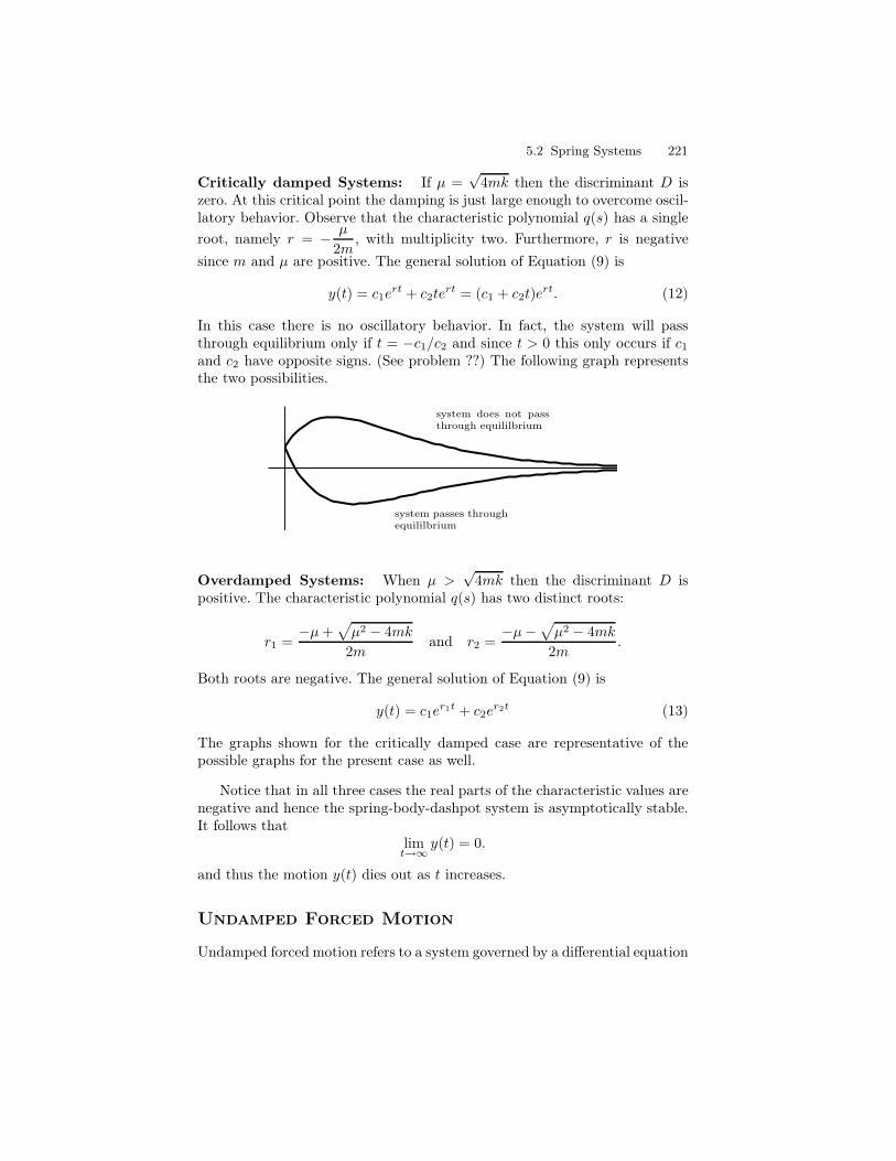
5.2 Spring Systems 221
Critically damped Systems: If µ =√
4mk then the discriminant D iszero. At this critical point the damping is just large enough to overcome oscil-latory behavior. Observe that the characteristic polynomial q(s) has a single
root, namely r = − µ
2m, with multiplicity two. Furthermore, r is negative
since m and µ are positive. The general solution of Equation (9) is
y(t) = c1ert + c2te
rt = (c1 + c2t)ert. (12)
In this case there is no oscillatory behavior. In fact, the system will passthrough equilibrium only if t = −c1/c2 and since t > 0 this only occurs if c1and c2 have opposite signs. (See problem ??) The following graph representsthe two possibilities.
system passes throughequililbrium
system does not passthrough equililbrium
Overdamped Systems: When µ >√
4mk then the discriminant D ispositive. The characteristic polynomial q(s) has two distinct roots:
r1 =−µ+
√
µ2 − 4mk
2mand r2 =
−µ−√
µ2 − 4mk
2m.
Both roots are negative. The general solution of Equation (9) is
y(t) = c1er1t + c2e
r2t (13)
The graphs shown for the critically damped case are representative of thepossible graphs for the present case as well.
Notice that in all three cases the real parts of the characteristic values arenegative and hence the spring-body-dashpot system is asymptotically stable.It follows that
limt→∞
y(t) = 0.
and thus the motion y(t) dies out as t increases.
Undamped Forced Motion
Undamped forced motion refers to a system governed by a differential equation
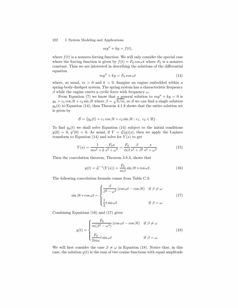
222 5 System Modeling and Applications
my′′ + ky = f(t),
where f(t) is a nonzero forcing function. We will only consider the special casewhere the forcing function is given by f(t) = F0 cosωt where F0 is a nonzeroconstant. Thus we are interested in describing the solutions of the differentialequation
my′′ + ky = F0 cosωt (14)
where, as usual, m > 0 and k > 0. Imagine an engine embedded within aspring-body-dashpot system. The spring system has a characteristic frequencyβ while the engine exerts a cyclic force with frequency ω.
From Equation (7) we know that a general solution to my′′ + ky = 0 isyh = c1 cosβt+ c2 sinβt where β =
√
k/m, so if we can find a single solutionyp(t) to Equation (14), then Theorem 4.1.8 shows that the entire solution setis given by
S = yp(t) + c1 cosβt+ c2 sinβt : c1, c2 ∈ R .
To find yp(t) we shall solve Equation (14) subject to the initial conditionsy(0) = 0, y′(0) = 0. As usual, if Y = L(y)(s), then we apply the Laplacetransform to Equation (14) and solve for Y (s) to get
Y (s) =1
ms2 + k
F0s
s2 + ω2=
F0
mβ
β
s2 + β2
s
s2 + ω2. (15)
Then the convolution theorem, Theorem 3.8.3, shows that
y(t) = L−1(Y (s)) =F0
mβsinβt ∗ cosωt. (16)
The following convolution formula comes from Table C.3:
sinβt ∗ cosωt =
β
β2 − ω2(cosωt− cosβt) if β 6= ω
1
2t sinωt if β = ω.
(17)
Combining Equations (16) and (17) gives
y(t) =
F0
m(β2 − ω2)(cosωt− cosβt) if β 6= ω
F0
2mωt sinωt if β = ω.
(18)
We will first consider the case β 6= ω in Equation (18). Notice that, in thiscase, the solution y(t) is the sum of two cosine functions with equal amplitude
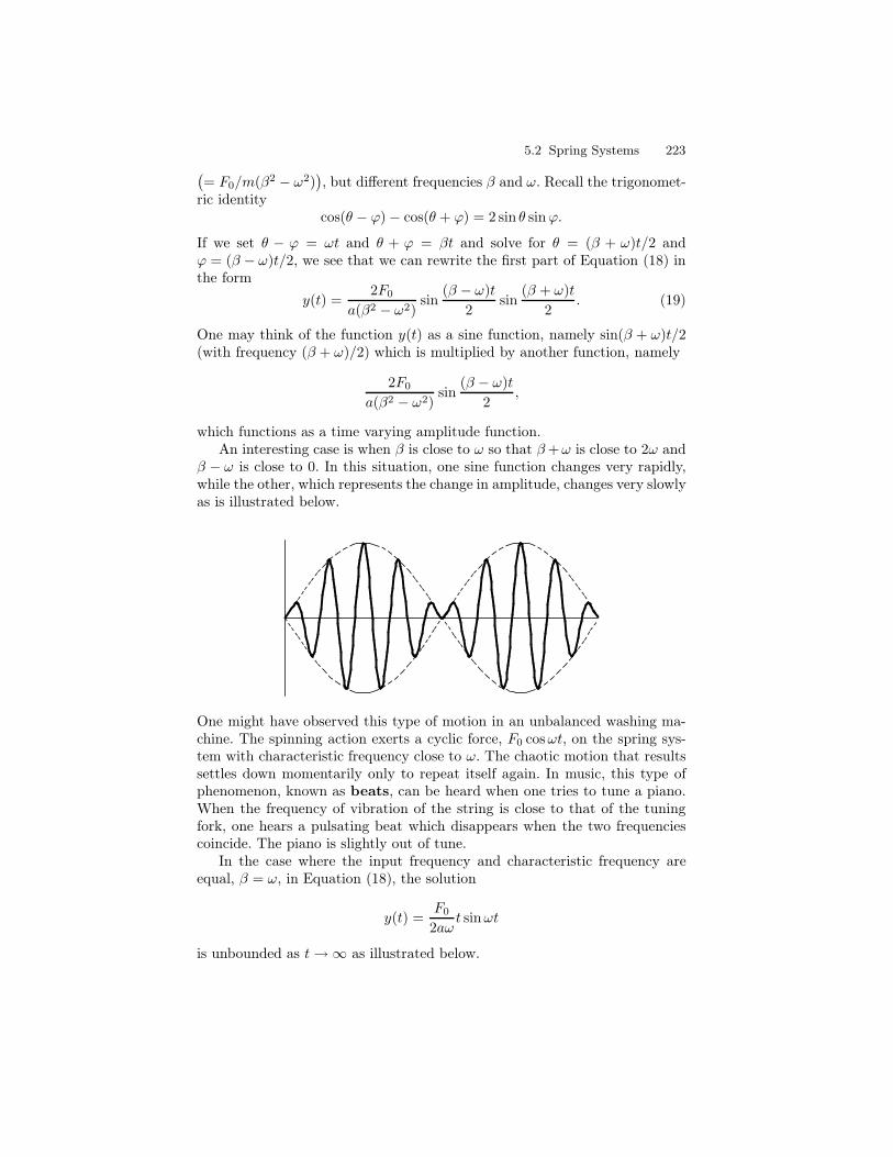
5.2 Spring Systems 223
(
= F0/m(β2 − ω2))
, but different frequencies β and ω. Recall the trigonomet-ric identity
cos(θ − ϕ)− cos(θ + ϕ) = 2 sin θ sinϕ.
If we set θ − ϕ = ωt and θ + ϕ = βt and solve for θ = (β + ω)t/2 andϕ = (β − ω)t/2, we see that we can rewrite the first part of Equation (18) inthe form
y(t) =2F0
a(β2 − ω2)sin
(β − ω)t
2sin
(β + ω)t
2. (19)
One may think of the function y(t) as a sine function, namely sin(β + ω)t/2(with frequency (β + ω)/2) which is multiplied by another function, namely
2F0
a(β2 − ω2)sin
(β − ω)t
2,
which functions as a time varying amplitude function.An interesting case is when β is close to ω so that β+ω is close to 2ω and
β − ω is close to 0. In this situation, one sine function changes very rapidly,while the other, which represents the change in amplitude, changes very slowlyas is illustrated below.
One might have observed this type of motion in an unbalanced washing ma-chine. The spinning action exerts a cyclic force, F0 cosωt, on the spring sys-tem with characteristic frequency close to ω. The chaotic motion that resultssettles down momentarily only to repeat itself again. In music, this type ofphenomenon, known as beats, can be heard when one tries to tune a piano.When the frequency of vibration of the string is close to that of the tuningfork, one hears a pulsating beat which disappears when the two frequenciescoincide. The piano is slightly out of tune.
In the case where the input frequency and characteristic frequency areequal, β = ω, in Equation (18), the solution
y(t) =F0
2aωt sinωt
is unbounded as t→∞ as illustrated below.
224 5 System Modeling and Applications
The resulting amplification of vibration eventually becomes large enough todestroy the mechanical system. This is a manifestation of resonance as dis-cussed in Section 5.1.
Damped Forced Motion
We now assume the damping constant µ is positive and consider forcing func-tions of the form f(t) = F0 cosωt where F0 is a constant, as before. Thus weare interested in analyzing the solutions of the equation
my′′ + µy′ + ky = F0 cosωt (20)
where m, µ, k and F0 are positive constants. It is a straightforward (albeittedious) calculation to check that the function
yp(t) =F0
(k − ω2m)2 + µ2ω2
(
(k − ω2m) cosωt+ µω sinωt)
is a solution of Equation (20). Using Equation (17), this can be rewritten as
yp(t) =F0
√
(k − ω2m)2 + µ2ω2cos(ωt− δ)
where tan δ =µω
k − ω2m. Combining this with Equation (??), the general
solution to Equation (??) is
y(t) = eαt(c1 cosβt+ c2 sinβt) +F0
√
(c− ω2a)2 + b2ω2cos(ωt− δ) (21)
where α = − b
2a< 0. Notice that this implies that limt→∞(y(t)− ϕp(t)) = 0,
which says that every general solution of Equation (??) converges asymptot-ically to the particular solution ϕp(t). For this reason, the solution ϕp(t) isusually referred to as the steady state solution to the equation, while the so-lution y(t) = eαt(c1 cosβt+ c2 sinβt) of the associated homogeneous equationis referred to as a transient solution.

5.3 Electrical Circuit Systems 225
5.3 Electrical Circuit Systems

6
Second Order Linear Differential Equations
In this chapter we consider the class of second order linear differential equa-tions. In particular, we will consider differential equations of the followingform:
a2(t)y′′ + a1(t)y
′ + a0(t)y = f(t). (1)
Notice that the coefficients a0(t), a1(t), and a2(t) are functions of the inde-pendent variable t and not necessarily constants. This difference has manyimportant consequences, the main one being that there is no general solutionmethod as in the constant coefficient case. Nevertheless, it is still linear and,as we shall see, this implies that the solution set has a structure similar to theconstant coefficient case.
In order to find solution methods one must put some rather strong restric-tions on the coefficient functions a0(t), a1(t) and a2(t). For example, in thefollowing list the coefficient functions are polynomial of a specific form. Theequations in this list are classical and have important uses in the physical andengineering sciences.
t2y′′ + ty′ + (t2 − ν2)y = 0 Bessel’s Equation of index ν
ty′′ + (1− t)y′ + λy = 0 Laguerre’s Equation of index λ
(1 − t2)y′′ − 2ty′ + α(α+ 1)y = 0 Legendre’s Equation of index α
(1 − t2)y′′ − ty′ + α2y = 0 Chebyshev’s Equation of index α
y′′ − 2ty′ + 2λy = 0 Hermite’s Equation of index λ
Except for a few simple cases the solutions to these equations are notexponential polynomials nor are they expressible in terms of algebraic com-binations of polynomials, trigonometric or exponential functions, nor theirinverses. Nevertheless, the general theory implies that solutions exist and tra-ditionally have been loosely categorized as special functions. In addition, tosatisfying the differential equation for the given index, there are other inter-
228 6 Second Order Linear Differential Equations
esting and important functional relations as the index varies. We will exploresome of these relations.
6.1 The Existence and Uniqueness Theorem
In this chapter we will assume that the coefficient functions a0(t), a1(t), anda2(t) and the forcing function f(t) are continuous functions on some com-mon interval I. We also assume that a2(t) 6= 0 for all t ∈ I. By dividing bya2(t), when convenient, we may assume that the leading coefficient functionis 1. In this case we say that the differential equation is in standard form.We will adopt much of the notation that we used in Section 4.1. In particular,let D denote the derivative operator and let
L = a2(t)D2 + a1(t)D + a0(t). (1)
Then Equation 1 in the introductory paragraph can be written as Ly = f . Theequation Ly = 0 is called homogeneous. Otherwise it is non homogeneous.We can think of L as an operation on functions. If y ∈ C2(I), in other words,if y is a function on an interval I having a second order continuous derivative,then Ly produces a continuous function.
Example 1. If L = D2 + 4tD + 1 then
• L(et) = (et)′′ + 4t(et)′ + 1(et) = (2 + 4t)et
• L(sin t) = − sin t+ 4t cos t+ sin t = 4t cos t
• L(t2) = 2 + 4t(2t) + (t2) = 9t2 + 2
• L(t+ 2) = 0 + 4t(1) + (t+ 2) = 5t+ 2
The most important property that we can say about L, generally, is thatit is linear.
Proposition 2. The operator
L = a2(t)D2 + a1(t)D + a0(t)
given by Equation 1 is linear. Specifically,
1. If y1 and y2 have second order continuous derivatives then
L(y1 + y2) = L(y1) + L(y2).
2. If y has a second order continuous derivative and c is a scalar then
L(cy) = cL(y).
6.1 The Existence and Uniqueness Theorem 229
Proof. The proof of this proposition is essentially the same as the proof ofProposition 4 in Section 4.1. We only need to remark that multiplication bya function ak(t) preserves addition and scalar multiplication in the same wayas multiplication by a constant ak.
We call L a second order linear differential operator. Proposition4.1.6 and Theorem 4.1.8 are two important consequences of linearity for theconstant coefficient case. The statement and proof are essentially the same forthe second order linear differential operators considered here in this chapter.We consolidate these results and the algorithm that followed into the followingtheorem:
Theorem 3. Suppose L is a second order linear differential operator and y1and y2 are solutions to Ly = 0. Then c1y1+c2y2 is a solution to Ly = 0, for allscalars c1 and c2. Suppose f is a continuous function. If yp is a fixed particularsolution to Ly = f and yh is any solution to the associated homogeneousdifferential equation Ly = 0 then
yp + yh
is a solution to Ly = f . Furthermore, any solution to Ly = f have this sameform. Thus to solve Ly = f we proceed as follows:
1. Find all the solutions to the associated homogeneous differential equationLy = 0,
2. Find one particular solution yp,3. Add the particular solution to the homogeneous solutions.
As an application of Theorem 3 consider the following example.
Example 4. Let L = tD2+2D+t. Show that sin tt and cos t
t are homogeneoussolutions. Show that t+1 is a solution to Ly = t2 + t+2. Use this informationand linearity to write the most general solution.
I Solution. It is a straightforward calculation to verify that sin tt and cos t
t
are homogeneous solutions. Theorem 3 now implies that c1 sin tt + c2
cos tt is a
homogeneous solution for all scalars c1 and c2. Again it is straightforward toverify that L(t+ 1) = t2 + t+ 2. Theorem 3 implies
y = t+ 1 + c1sin t
t+ c2
cos t
t
is a solution and we will soon see it is the general solution. J
Again, suppose L is a second order linear differential operator and f is afunction defined on an interval I. Let t0 ∈ I. To the equation
Ly = f
230 6 Second Order Linear Differential Equations
we can associate initial conditions of the form
y(t0) = y0, and y′(t0) = y1.
We refer to the initial conditions and the differential equation Ly = f as aninitial value problem.
Example 5. Let L = tD2 + 2D + t. Solve the initial value problem
Ly = t2 + t+ 2, y(π) = 1, y′(π) = 1.
I Solution. By Example 4 the general solution is of the form y = t + 1 +c1
sin tt + c2
cos tt . The initial conditions lead to the equations
π + 1− c2π
= 1
1− c1π
+1
π= 1,
which imply c1 = π and c2 = π2. The solution to the initial value problem is
y = t+ 1 + πsin t
t+ π2 cos t
t.
J
In the case where the coefficient functions of L are constant we proved theexistence and uniqueness theorem by an inductive method in Section 4.2. Theinductive method relied on factoring L, which is not always possible in thepresent, more general, context. Nevertheless, we still have the existence anduniqueness theorem. Its proof is beyond the scope of this book. We refer toCoddington [?] for a proof and more detailed information.
Theorem 6. Suppose a0(t), a1(t), a2(t) and f are continuous functions onan open interval I and an(t) 6= 0 for all t ∈ I. Suppose t0 ∈ I. Let L =a2(t)D
2 + a1(t)D + a0(t). Then there is one and only one solution to theinitial value problem
Ly = f, y(t0) = y0, y′(t0) = y1.
Theorem 6 does not tell us how to find any solution. We must developprocedures for this. Let’s explain in more detail what this theorem does say.Under the conditions stated the Uniqueness and Existence theorem says thatthere always is a solution to the given initial value problem. The solution is atleast twice differentiable on I and there is no other solution. In Example 5 wefound y = t+1+π sin t
t +π2 cos tt is a solution to ty′′+2y′+ ty = t2 + t+2. with
initial conditions y(π) = 2 and y′(π) = 1. Notice, in this case, that y is, in fact,infinitely differentiable on any interval not containing 0. This is precisely wherea2(t) = t is zero. The uniqueness part of Theorem 6 implies that there are no
6.1 The Existence and Uniqueness Theorem 231
other solutions. In other words, there are no potentially hidden solutions, sothat if we can find enough solutions to take care of all possible initial values,then Theorem 6 provides the theoretical underpinnings to know that we havefound all possible solutions and need look no further. Compare this theoremwith the discussion in Section 2.3 where we saw examples (in the nonlinearcase) of initial value problems which had infinitely many distinct solutions.
Exercises
1–12. For each of the following dif-ferential equations, determine if it islinear (yes/no). For each of thosewhich is linear, further determine ifthe equation is homogeneous (homo-geneous/nonhomogeneous) and constantcoefficient (yes/no). Do not solve theequations.
1. y′′ + y′y = 0
2. y′′ + y′ + y = 0
3. y′′ + y′ + y = t2
4. y′′ + ty′ + (1 + t2)y2 = 0
5. 3y′′ + 2y′ + y = e2
6. 3y′′ + 2y′ + y = et
7. y′′ +√
y′ + y = t
8. y′′ + y′ + y =√
t
9. y′′ − 2y = ty
10. y′′ + 2y + t sin y = 0
11. y′′ + 2y′ + (sin t)y = 0
12. t2y′′ + ty′ + (t2 − 5)y = 0
13–18. For each of the following lineardifferential operators L compute L(1),L(t), L(e−t), and L(cos 2t). That is,evaluate L(y) for each of the given inputfunctions.
13. L(y) = y′′ + y
14. L(y) = ty′′ + y
15. L(y) = 2y′′ + y′ − 3y
16. L = D2 + 6D + 5
17. L = D2 − 4
18. L = t2D2 + tD − 1
19. If L = aD2 + bD + c where a, b,c are real numbers, then show thatL(ert) = (ar2 + br + c)ert. Thatis, the effect of applying the oper-ator L to the exponential functionert is to multiply ert by the numberar2 + br + c.
20. The differential equation t2y′′+ty′−y = t
12 , t > 0 has a solution of the
form ϕp(t) = Ct12 . Find C.
21. The differential equation y′′ + 3y′ +2y = t has a solution of the formϕp(t) = C1 + C2t. Find C1 and C2.
22. Does the differential equation y′′ +3y′ +2y = e−t have a solution of theform ϕp(t) = Ce−t? If so find C.
23. Does the differential equation y′′ +3y′ +2y = e−t have a solution of theform ϕp(t) = Cte−t? If so find C.Let L(y) = y′′ + y.
24–26.
24. Let L(y) = y′′ + y
1. Check that y(t) = t2 − 2 is onesolution to the differential equa-tion L(y) = t2.
232 6 Second Order Linear Differential Equations
2. Check that y1(t) = cos t andy2(t) = sin t are two solutions tothe differential equation L(y) =0.
3. Using the results of Parts (a)and (b), find a solution to eachof the following initial valueproblems.a) y′′ + y = t2, y(0) = 1,
y′(0) = 0.
b) y′′ + y = t2, y(0) = 0,y′(0) = 1.
c) y′′ + y = t2, y(0) = −1,y′(0) = 3.
d) y′′ + y = t2, y(0) = a,y′(0) = b, where a, b ∈ R.
25. Let L(y) = y′′ − 5y′ + 6y.1. Check that y(t) = 1
2et is one
solution to the differential equa-tion L(y) = et.
2. Check that y1(t) = e2t andy2(t) = e3t are two solutions tothe differential equation L(y) =0.
3. Using the results of Parts (1)and (2), find a solution to eachof the following initial valueproblems.a) y′′−5y′ +6y = et, y(0) =
1, y′(0) = 0.
b) y′′−5y′ +6y = et, y(0) =0, y′(0) = 1.
c) y′′−5y′ +6y = et, y(0) =−1, y′(0) = 3.
d) y′′−5y′ +6y = et, y(0) =a, y′(0) = b, where a, b ∈R.
26. Let L(y) = t2y′′ − 4ty′ + 6y.1. Check that y(t) = 1
6t5 is one
solution to the differential equa-tion L(y) = t5.
2. Check that y1(t) = t2 andy2(t) = t3 are two solutions tothe differential equation L(y) =0.
3. Using the results of Parts (a)and (b), find a solution to eachof the following initial valueproblems.a) t2y′′ − 4ty′ + 6y = t5,
y(1) = 1, y′(1) = 0.
b) t2y′′ − 4ty′ + 6y = t5,y(1) = 0, y′(1) = 1.
c) t2y′′ − 4ty′ + 6y = t5,y(1) = −1, y′(1) = 3.
d) t2y′′ − 4ty′ + 6y = t5,y(1) = a, y′(1) = b, wherea, b ∈ R.
27–32. For each of the following differ-ential equations, find the largest inter-val on which a unique solution of theinitial value problem a0(t)y
′′ + a1(t)y′ +
a3(t)y = f(t), y(t0) = y1, y′(t0) = y1
is guaranteed by Theorem 6. Note thatyour interval may depend on the choiceof t0.
27. t2y′′ + 3ty′ − y = t4
28. y′′ − 2y′ − 2y =1 + t2
1 − t2
29. (sin t)y′′ + y = cos t
30. (1 + t2)y′′ − ty′ + t2y = cos t
31. y′′ +√
ty′ −√
t − 3y = 0
32. t(t2 − 4)y′′ + y = et
33. The functions y1(t) = t2 and y2(t) =t3 are two distinct solutions of theinitial value problem
t2y′′−4ty′+6y = 0, y(0) = 0, y′(0) = 0.
Why doesn’t this violate the unique-ness part of Theorem 6?
34. Let y(t) be a solution of the differ-ential equation
y′′ + a1(t)y′ + a0(t)y = 0.
We assume that a1(t) and a0(t) arecontinuous functions on an intervalI , so that Theorem 6 implies thaty is defined on I . Show that if thegraph of y(t) is tangent to the t-axis
6.2 The Homogeneous Case 233
at some point t0 of I , then y(t) = 0for all t ∈ I . Hint: If the graph ofy(t) is tangent to the t-axis at (t0, 0),what does this say about y(t0) andy′(t0)?
35. More generally, let y1(t) and y2(t)be two solutions of the differentialequation
y′′ + a1(t)y′ + a0(t)y = f(t),
where, as usual we assume thata1(t), a0(t), and f(t) are continuousfunctions on an interval I , so thatTheorem 6 implies that y1 and y2
are defined on I . Show that if thegraphs of y1(t) and y2(t) are tan-gent at some point t0 of I , theny1(t) = y2(t) for all t ∈ I .
6.2 The Homogeneous Case
In this section we are mainly concerned with the homogeneous case:
L(y) = a2(t)y′′ + a1(t)y
′ + a0(t)y = 0 (1)
The main result, Theorem 4 given below, shows that we will in principle beable to find two functions y1 and y2 such that all solutions to Equation (1)are of the form c1y1 + c2y2, for some constants c1 and c2. This is just likethe second order constant coefficient case. In fact, if q(s) is a characteristicpolynomial of degree 2 then Bq = y1, y2 is a set of two linearly indepen-dent functions that span the solution set of the corresponding homogeneousconstant coefficient differential equation. In section 3.7 we introduced the con-cept of linear independence for a set of n functions. Let’s recall this importantconcept in the case n = 2.
Linear Independence
Two functions y1 and y2 defined on some interval I are said to be linearlyindependent if the equation
c1y1 + c2y2 = 0 (2)
implies that c1 and c2 are both 0. Otherwise, we call y1 and y2 linearlydependent.
One must be careful about the meaning of this definition. We do not trysolve Equation (2) for the variable t. Rather, we are given that this equationis valid for all t ∈ I. With this information the focus is on what this saysabout the constants c1 and c2: are they necessarily both zero or not.
Let’s consider two examples.
234 6 Second Order Linear Differential Equations
Example 1. Let y1(t) = t and y2(t) = t2 be defined on I = R. If theequation
c1t+ c2t2 = 0,
is valid for all t ∈ R, then this implies, in particular, that
c1 + c2 = 0 (let t = 1)
−c1 + c2 = 0 (let t = −1)
Now this system of linear equations is easy to solve. We obtain c1 = 0 andc2 = 0. Thus t and t2 are linearly independent.
Example 2. In this second example let y1(t) = t and y2(t) = −2t definedon I = R. Then there are many sets of constants c1 and c2 such that c1t +c2(−2t) = 0. For example, we could choose c1 = 2 and c2 = 1. So the equationc1t+ c2(−2t) = 0 does not necessarily mean that c1 and c2 are zero. Hence tand −2t are not independent. They are linearly dependent.
Remark 3. Notice that y1 and y2 are linearly dependent precisely when onefunction is a scalar multiple of the other, i.e., y1 = αy2 or y2 = βy1 forα ∈ R or β ∈ R. In Example 1, y2 6= cy1 while in Example 2, y2 = −2y1.Furthermore, given two linearly independent functions neither of them can bezero.
The main theorem for the homogeneous case
Theorem 4. Let L = a2(t)D2 +a1(t)D+a0(t), where a0(t), a1(t), and a2(t)
are continuous functions on an interval I. Assume a2(t) 6= 0 for all t ∈ I.1. There are two linearly independent solutions to Ly = 0.2. If y1 and y2 are independent solution Ly = 0 then any homogeneous so-
lution y can be written y = c1y1 + c2y2, for some c1, c2 ∈ R.
Proof. Let t0 ∈ I. By Theorem 6, there are functions, ψ1 and ψ2, that aresolutions to the initial value problems L(y) = 0, with initial conditions y(t0) =1, y′(t0) = 0 and y(t0) = 0, y′(t0) = 1, respectively. Suppose c1ψ1 +c2ψ2 = 0.Then
c1ψ1(t0) + c2ψ2(t0) = 0.
Since ψ1(t0) = 1 and ψ2(t0) = 0 it follows that c1 = 0. Similarly we have,
c1ψ′1(t0) + c2ψ
′2(t0) = 0.
Since ψ′1(t0) = 0 and ψ′
2(t0) = 1 it follows that c2 = 0. Therefore ψ1 and ψ2
are linearly independent. This proves (1).Suppose y is a homogeneous solution. Let r = y(t0) and s = y′(t0). By
Theorem 3 the function rψ1 + sψ2 is a solution to Ly = 0. Furthermore,
6.2 The Homogeneous Case 235
rψ1(t0) + sψ2(t0) = r
and rψ′1(t0) + sψ′
2(t0) = s.
This means the rψ1 + sψ2 and y satisfy the same initial conditions. By theuniqueness part of Theorem 6 they are equal. Thus y = rψ1 + sψ2, i.e., everyhomogeneous solution is a linear combination of ψ1 and ψ2.
Now suppose y1 and y2 are any two linearly independent homogeneoussolutions and suppose y is any other solution. From the argument above wecan write
y1 = aψ1 + bψ2
y2 = cψ1 + dψ2,
which in matrix form can be written[
y1y2
]
=
[
a bc d
] [
ψ1
ψ2
]
.
We multiply both sides of this matrix equation by the adjoint
[
d −b−c a
]
to
obtain[
d −b−c a
] [
y1y2
]
=
[
ad− bc 00 ad− bc
] [
ψ1
ψ2
]
= (ad− bc)[
ψ1
ψ2
]
.
Suppose ad− bc = 0. Then
dy1 − by2 = 0
and − cy1 + ay2 = 0.
But since y1 and y2 are independent this implies that a, b, c, and d are zerowhich in turn implies that y1 and y2 are both zero. But this cannot be. Weconclude that ad − bc 6= 0. We can now write ψ1 and ψ2 each as a linearcombination of y1 and y2. Specifically,
[
ψ1
ψ2
]
=1
ad− bc
[
d −b−c a
] [
y1y2
]
.
Since y is a linear combination of ψ1 and ψ2 it follows the y is a linear com-bination of y1 and y2. ut
Remark 5. The matrix
[
a bc d
]
that appears in the proof above appears in
other contexts as well. If y1 and y2 are homogeneous solutions to Ly = 0 wedefine the Wronskian matrix by
W (y1, y2)(t) =
[
y1(t) y2(t)y′1(t) y
′2(t)
]
236 6 Second Order Linear Differential Equations
and the Wronskian by
w(y1, y2)(t) = detW (y1, y2).
The relations
y1 = aψ1 + bψ2
y2 = cψ1 + dψ2,
in the proof, when evaluated at t0 imply that[
a bc d
]
=
[
y1(t0) y′1(t0)
y1(t0) y′2(t0)
]
= W (y1, y2)t(t0).
Since it was shown that ad− bc 6= 0 we have shown the following proposi-tion.
Proposition 6. Suppose L satisfies the conditions of Theorem 4. Suppose y1and y2 are linearly independent solutions to Ly = 0. Then
w(y1, y2) 6= 0.
On the other hand, given any two differentiable functions, y1 and y2, (notnecessarily homogeneous solutions) whose Wronskian is a nonzero functionthen it is easy to see that y1 and y2 are independent. For suppose, t0 is chosenso that w(y1, y2)(t0) 6= 0 and c1y1 + c2y2 = 0. Then c1y
′1 + c2y
′2 = 0 and we
have[
00
]
=
[
c1y1(t0) + c2y2(t0)c1y
′1(t0) + c2y
′2(t0)
]
= W (y1, y2)
[
c1c2
]
.
Simple matrix algebra 1 gives c1 = 0 and c2 = 0. Hence y1 and y2 are linearlyindependent.
Although one could check independence in this way it is simpler and moreto the point to use the observation given in Remark 3.
Remark 7. Let’s now summarize what Theorems 6.1.3, 6.1.6, and 4 tell us.In order to solve L(y) = f (satisfying the continuity hypotheses) we first needto find a particular solution yp, which exists by the Uniqueness and ExistenceTheorem 6. Next, Theorem 4 says that if y1 and y2 are any two linearlyindependent solutions of the associated homogeneous equation L(y) = 0, thenall of the solutions of the associated homogeneous equation are of the formc1y1 + c2y2. Theorem 3 now tells us that all solutions to L(y) = f are of theform yp + c1y1 + c2y2 for some choice of the constants c1 and c2. Furthermore,any set of initial conditions uniquely determine the constants c1 and c2.
1c.f. Chapter 9 for a discussion of matrices
6.2 The Homogeneous Case 237
A set y1, y2 of linearly independent solutions to the homogeneous equa-tion L(y) = 0 is called a fundamental set for the second order linear differ-ential operator L. A fundamental set is a basis of the linear space of homoge-neous solutions (c.f. Section 3.7 for the definition of a basis). Furthermore, thestandard basis, Bq, in the context of constant coefficient differential equations,is a fundamental set.
In the following sections we will develop methods, under suitable assump-tions, for finding a fundamental set for L and a particular solution to thedifferential equation L(y) = f . For now, let’s illustrate the main theoremswith an example.
Example 8. Consider the differential equation
t2y′′ + ty′ + y = 2t.
Suppose
• A particular solution is yp(t) = t.• Two independent solutions of the homogeneous equation L(y) = 0 are
y1(t) = cos(ln t) and y2(t) = sin(ln t).
Determine the solution set and the largest interval on which these solutionsare valid.
I Solution. In this case we divide by t2 to rewrite the equation in standardform as y′′ + (1/t)y′ + (1/t2)y = 2/t and observe that the coefficients arecontinuous on the interval (0,∞). Here L = D2 + (1/t)D + (1/t2) and theforcing function is f(t) = 1/t2. It is easy to see that cos(ln t), sin(ln t) islinearly independent and thus a fundamental set for L(y) = 0. It now followsthat the solution set to L(y) = f is given by
t+ c1 cos(ln t) + c2 sin(ln t) : c1, c2 ∈ R .
J
Exercises
1–8. Determine if each of the followingpairs of functions are linearly indepen-dent or linearly dependent.
1. y1(t) = 2t, y2(t) = 5t
2. y1(t) = t2, y2(t) = t5
3. y1(t) = e2t, y2(t) = e5t
4. y1(t) = e2t+1, y2(t) = e2t−3
5. y1(t) = ln(2t), y2(t) = ln(5t)
6. y1(t) = ln t2, y2(t) = ln t5
7. y1(t) = sin 2t, y2(t) = sin t cos t
8. y1(t) = cosh t, y2(t) = 3et(1+e−2t)
9. 1. Verify that y(t) = t3 and y2(t) =|t3| are linearly independent on(−∞, ∞).
238 6 Second Order Linear Differential Equations
2. Show that the Wronskian,w(y1, y2)(t) = 0 for all t ∈ R.
3. Explain why Parts (a) and (b)do not contradict Proposition 6.
4. Verify that y1(t) and y2(t) aresolutions to the linear differen-
tial equation t2y′′ − 2ty′ = 0,y(0) = 0, y′(0) = 0.
5. Explain why Parts (a), (b),and (d) do not contradict theUniqueness and Existence theo-rem, Theorem 6 of Section 6.1.
6.3 The Cauchy-Euler Equations
When the coefficient functions of a second order linear differential equation arenonconstant the corresponding equation can become very difficult to solve. Inorder to expect to find solutions one must put certain restrictions on the coeffi-cient functions. A class of nonconstant coefficient linear differential equations,known as Cauchy-Euler equations, have solutions that are easy to obtain.
A Cauchy-Euler equation is a second order linear differential equationof the following form:
at2y′′ + bty′ + cy = 0, (1)
where a, b and c are real constants and a 6= 0. When put in standard form weobtain:
y′′ +b
aty′ +
c
at2y = 0.
The functions bat and c
at2 are continuous everywhere except at 0. Thus by theUniqueness and Existence Theorem solutions exist in either of the intervals(−∞, 0) or (0,∞). Of course, a solution need not, and in general, will notexist on the entire real line R. To work in a specific interval we will assumet > 0. We will refer to L = at2D2 + btD + c as a Cauchy-Euler operator.
The Laplace transform method does not work in any simple fashion here.However, the simple change in variable t = ex will transform Equation (1) intoa constant coefficient linear differential equation. To see this let Y (x) = y(ex).Then the chain rule gives
Y ′(x) = exy′(ex)
and Y ′′(x) = exy′(ex) + (ex)2y′′(ex)
= Y ′(x) + (ex)2y′′(ex).
Thus
a(ex)2y′′(ex) = aY ′′(x) − aY ′(x)
bexy′(ex) = bY ′(x)
cy(ex) = cY (x).
6.3 The Cauchy-Euler Equations 239
Addition of these terms gives
a(ex)2y′′(ex) + bexy′(ex) + cy(ex) = aY ′′(x)− aY ′(x) + bY ′(x) + cY (x)
= aY ′′(x) + (b − a)Y ′(x) + cY (x).
With t replaced by ex in Equation 1 we now obtain
aY ′′(x) + (b− a)Y ′(x) + cY (x) = 0. (2)
The polynomialq(s) = as2 + (b− a)s+ c
is the characteristic polynomial of Equation 2 and known as the indicialpolynomial of Equation 1. Equation (2) is a second order constant coefficientdifferential equation and by now routine to solve. Its solutions depends on theway q(s) factors. We consider the three possibilities.
q has distinct real roots
Suppose r1 and r2 are distinct roots to the indicial polynomial q(s). Thener1x and er2x are solutions to Equation (2). Solutions to Equation (1) areobtained by the substitution x = ln t: we have er1x = er1 ln t = tr1 and similarlyer2x = tr2 . Since tr1 is not a multiple of tr2 they are independent and hencetr1 , tr2 is a fundamental set for L(y) = 0.
Example 1. Find a fundamental set for the equation t2y′′ − 2y = 0.
I Solution. The indicial polynomial is s2−s−2 = (s−2)(s+1) and it has 2and −1 as roots and thus
t2, t−1
is a fundamental set for this Cauchy-Eulerequation. J
q has a double root
Suppose r is a double root of q. Then erx and xerx are independent solutions toEquation (2). The substitution x = ln t then gives tr and tr ln t as independentsolutions to Equation (1). Hence tr, tr ln t is a fundamental set for L(y) = 0.
Example 2. Find a fundamental set for the equation 4t2y′′ + 8ty′ + y = 0.
I Solution. The indicial polynomial is 4s2 +4s+1 = (2s+1)2 and has − 12
as a root with multiplicity 1. Thus
t−12 , t−
12 ln t
is a fundamental set. J
240 6 Second Order Linear Differential Equations
q has conjugate complex roots
Suppose q has complex roots α ± iβ, where β 6= 0. Then eαx cosβx andeαx sinβx are independent solutions to Equation (2). The substitution x = ln tthen gives tα cos(β ln t), tα sin(β ln t) as a fundamental set for Ly = 0.
Example 3. Find a fundamental set for the equation t2y′′ + ty′ + y = 0.
I Solution. The indicial polynomial is s2+1 which has ±i as complex roots.Theorem 4 implies that cos ln t, sin ln t is a fundamental set. J
We now summarize the above results into one theorem.
Theorem 4. Let L = at2D2 + btD + c, where a, b, c ∈ R and a 6= 0. Letq(s) = as2 + (b− a)s+ c be the indicial polynomial.
1. If r1 and r2 are distinct real roots of q(s) then
tr1 , tr2
is a fundamental set for L(y) = 0.2. If r is a double root of q(s) then
tr, tr ln t
is a fundamental set for L(y) = 0.3. If α± iβ are complex conjugate roots of q(s), β 6= 0 then
tα sin(β ln t), tα cos(β ln t)
is a fundamental set for L(y) = 0.
Exercises
1–11. Find the general solution of eachof the following homogeneous Cauchy-Euler equations on the interval (0, ∞).
1. t2y′′ + 2ty′ − 2y = 0
2. 2t2y′′ − 5ty′ + 3y = 0
3. 9t2y′′ + 3ty′ + y = 0
4. t2y′′ + ty′ − 2y = 0
5. 4t2y′′ + y = 0
6. t2y′′ − 3ty′ − 21 = 0
7. t2y′′ + 7ty′ + 9y = 0
8. t2y′′ − y = 0
9. t2y′′ + ty′ − 4y = 0
10. t2y′′ + ty′ + 4y = 0
11. t2y′′ − 3ty′ + 13y = 0
12–15. Solve each of the following ini-tial value problems.
6.4 Laplace Transform Methods 241
12. t2y′′ + 2ty′ − 2y = 0, y(1) = 0,y′(1) = 1
13. 4t2y′′+y = 0, y(1) = 2, y′(1) =0
14. t2y′′ + ty′ + 4y = 0, y(1) = −3,y′(1) = 4
15. t2y′′ − 4ty′ + 6y = 0, y(0) = 1,y′(0) = −1
6.4 Laplace Transform Methods
In this section we will develop some further properties of the Laplace transformand use them to solve some linear differential equations with non constantcoefficient functions. The use of the Laplace transform is limited, however, aswe shall see.
To begin with we need to consider a class of functions wider than theexponential-polynomials. A continuous function f on [0,∞) is said to be ofexponential type with order a if there is a constant K such that
|f(t)| ≤ Keat
for all t ∈ [0,∞). If the order is not important to the discussion we will just sayf is of exponential type. This definition applies to both real and complexvalued functions. The idea here is to limit the kind of growth that we allowf to have; it cannot grow faster than a multiple of an exponential function.The above inequality means
−Keat ≤ f(t) ≤ Keat,
for all t ∈ [0,∞) as illustrated in Figure 6.1, where the boldfaced curve, f(t),lies between the upper and lower exponential functions.
As we will see below, limiting growth in this way will assure us that fhas a Laplace transform. It is an easy exercise to show that the sum andproduct of functions of exponential type are again of exponential type. Alsoany continuous bounded function on [0,∞) is of exponential type. Since tn ≤ent for t ≥ 0 it follows that
∣
∣tneλt∣
∣ ≤ e(n+a)t, where a = Reλ. Hence, theexponential-polynomials are of exponential type and thus everything we sayabout functions of exponential type applies to the exponential-polynomials.
Proposition 1. Let f be of exponential type with order a. Then the Laplacetransform Lf(t)(s) exists for all s > a.
Proof. Let f be exponential type of order a. Then |f | ≤ Keat for some K and∣
∣
∣
∣
∫ ∞
0
e−stf(t) dt
∣
∣
∣
∣
≤∫ ∞
0
e−st |f(t)| dt ≤ K∫ ∞
0
e−(s−a)t dt =K
s− a ,
provided s > a. ut
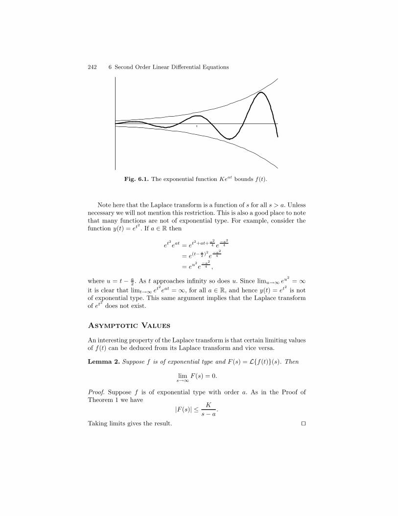
242 6 Second Order Linear Differential Equations
t
Fig. 6.1. The exponential function Keat bounds f(t).
Note here that the Laplace transform is a function of s for all s > a. Unlessnecessary we will not mention this restriction. This is also a good place to notethat many functions are not of exponential type. For example, consider thefunction y(t) = et2 . If a ∈ R then
et2eat = et2+at+ a2
4 e−a2
4
= e(t−a2 )2e
−a2
4
= eu2
e−a2
4 ,
where u = t − a2 . As t approaches infinity so does u. Since limu→∞ eu2
= ∞it is clear that limt→∞ et2eat = ∞, for all a ∈ R, and hence y(t) = et2 is notof exponential type. This same argument implies that the Laplace transformof et2 does not exist.
Asymptotic Values
An interesting property of the Laplace transform is that certain limiting valuesof f(t) can be deduced from its Laplace transform and vice versa.
Lemma 2. Suppose f is of exponential type and F (s) = Lf(t)(s). Then
lims→∞
F (s) = 0.
Proof. Suppose f is of exponential type with order a. As in the Proof ofTheorem 1 we have
|F (s)| ≤ K
s− a .
Taking limits gives the result. ut
6.4 Laplace Transform Methods 243
Theorem 3 (Initial Value Theorem). Suppose f and its derivative f ′ areof exponential order. Let F (s) = Lf(t)(s). Then
Initial Value Principle
f(0) = lims→∞
sF (s).
Proof. Let H(s) = Lf ′(t)(s). By Lemma 2 we have
0 = lims→∞
H(s) = lims→∞
(sF (s)− f(0)) = lims→∞
(sF (s)− f(0)).
This implies the result. ut
Example 4. Verify the Initial Value Theorem for f(t) = cos at.
I Solution. On the one hand, cos at|t=0 = 1. On the other hand,
sLcos at(s) =s2
s2 + a2
which has limit 1 as s→∞. J
Theorem 5 (Final Value Theorem). Suppose f and f ′ are of exponentialtype and limt→∞ f(t) exists. If F (s) = Lf(t)(s) then
Final Value Principle
limt→∞
f(t) = lims→0
sF (s).
Proof. Let H(s) = Lf ′(t)(s) = sF (s) − f(0). Then sF (s) = H(s) + f(0)and
lims→0
sF (s) = lims→0
H(s) + f(0)
= lims→0
limM→∞
∫ M
0
e−stf ′(t) dt+ f(0)
= limM→∞
∫ M
0
f ′(t) dt+ f(0)
= limM→∞
f(M)− f(0) + f(0)
= limM→∞
f(M).
ut
244 6 Second Order Linear Differential Equations
Integration in Transform Space
The Transform Derivative Principle, Theorem 3.1.16, tells us that multiplica-tion by −t induces differentiation of the Laplace transform. One might expectthen that division by −t will induce integration in the transform space. Thisidea is valid but we must be careful about assumptions. First if f(t) has aLaplace transform it is not necessarily the case that f(t)/t will likewise. Forexample, the constant function f(t) = 1 has Laplace transform 1
s but f(t)t = 1
tdoes not have a Laplace transform. Second, integration produces an arbitraryconstant of integration. What is this constant? The precise statement is asfollows:
Theorem 6 (Integration in Transform Space). Suppose f is of exponen-
tial type with order a and f(t)t has a continuous extension to 0, i.e. limt→0+
f(t)t
exists. Then f(t)t is of exponential type with order a and
Tranform Integral Principle
L
f(t)t
(s) =∫∞
s F (σ) dσ,
where s > a.
Proof. Let L = limt→0+f(t)
t and define
h(t) =
f(t)t if t > 0
L if t = 0.
Since f is continuous so is h. Since f is of exponential type with order a thereis a K so that |f(t)| ≤ Keat. Since 1
t ≤ 1 on [1,∞)
|h(t)| =∣
∣
∣
∣
f(t)
t
∣
∣
∣
∣
≤ |f(t)| ≤ Keat,
for all t ≥ 1. Since h is continuous on [0, 1] it is bounded by B, say. Thus|h(t)| ≤ B ≤ Beat for all t ∈ [0, 1]. If M is the larger of K and B then
|h(t)| ≤Meat,
for all t ∈ [0,∞) and hence h is of exponential type. Let H(s) = Lh(t)(s)and F (s) = Lf(t) (s). Then, since −th(t) = −f(t) we have, by Theorem3.1.16, H ′(s) = −F (s). Thus H is an antiderivative of −F and we have
H(s) = −∫ s
a
F (σ) dσ + C.
6.4 Laplace Transform Methods 245
Lemma 2 implies 0 = lims→∞H(s) = −∫∞
aF (σ) dσ + C and hence C =
∫∞aF (σ) dσ. Therefore
L
f(t)
t
(s) = H(s)
=
∫ a
s
F (σ) dσ +
∫ ∞
a
F (σ) dσ
=
∫ ∞
s
F (σ) dσ.
ut
The Laplace transform of several new functions can now be deduced fromthis theorem. Consider an example.
Example 7. Find L
sin tt
.
I Solution. Since limt→0sin t
t = 1 Theorem 6 applies to give
L
sin t
t
(s) =
∫ ∞
s
1
σ2 + 1dσ
= tan−1 σ|∞s=π
2− tan−1(s)
= tan−1 1
s.
J
Solving Linear Differential Equations
We now consider by example how one can use the Laplace transform methodto solve some differential equations.
Example 8. Find a solution of exponential type that solves
ty′′ − (1 + t)y′ + y = 0.
I Solution. Note that the Existence and Uniqueness theorem implies thatsolutions exist on intervals that do not contain 0. We presume that such asolution has a continuous extension to t = 0 and is of exponential type. Let ybe such a solution. Let y(0) = y0, y′(0) = y1 and Y (s) = Ly(t) (s). Appli-cation of Transform Derivative Principle, Theorem 3.116, to each componentof the differential equation gives
246 6 Second Order Linear Differential Equations
Lty′′ = −(s2Y (s)− sy(0)− y′(0))′
= −(2sY (s) + s2Y ′(s)− y(0))
L−(1 + t)y′ = L−y′+ L−ty′= −sY (s) + y0 + (sY (s)− y0)′= sY ′(s)− (s− 1)Y (s) + y0
Ly = Y (s).
The sum of the left-hand terms is given to be 0. Thus adding the right-handterms and simplifying gives
(s− s2)Y ′(s) + (−3s+ 2)Y (s) + 2y0 = 0,
which can be rewritten in the following way:
Y ′(s) +3s− 2
s(s− 1)Y (s) =
2y0s(s− 1)
.
This equation is a first order linear differential equation in Y (s). Since 3s−2s(s−1) =
2s + 1
s−1 it is easy to see that an integrating factor is I = s2(s− 1) and hence
(IY (s))′ = 2y0s.
Integrating and solving for Y gives
Y (s) =y0s− 1
+c
s2(s− 1).
The inverse Laplace transform is y(t) = y0et + c(et− t− 1). For simplicity, we
can write this solution in the form
y(t) = Aet +B(t+ 1),
where A = y0 +c and B = −c. It is easy to verify that et and t+1 are linearlyindependent and solutions to the given differential equation. J
Example 9. Find a solution of exponential type that solves
ty′′ + 2y′ + ty = 0.
I Solution. Again, assume y is a solution of exponential type. Let Y (s) =Ly(t)(s). As in the preceding example we apply the Laplace transform andsimplify. The result is a simple linear differential equation:
Y ′(s) =−y0s2 + 1
.
Integration gives Y (s) = y0(− tan−1 s + C). By Lemma 2 we have 0 =lims→∞ Y (s) = y0(−π
2 + C) which implies C = π2 and
6.4 Laplace Transform Methods 247
Y (s) = y0(π
2− tan−1 s) = y0 tan−1 1
s.
By Example 7 we get
y(t) = y0sin t
t.
J
Theorem 6.2.4 implies that there are two linearly independent solutions.The Laplace transform method has found only one, namely, sin t
t . In the Sec-tion 6.5 we will introduce a technique that will find another independentsolution. When applied to this example we will find y(t) = cos t
t is anothersolution. (c.f. Example 6.1.4.) It is easy to check that the Laplace transformof cos t
t does not exist and thus the Laplace transform method cannot find itas a solution. Furthermore, the constant of integration, C, in this examplecannot be arbitrary, because of Lemma 2. It frequently happens in examplesthat C must be carefully chosen.
We observe that the presence of the linear factor t in Examples 8 and 9produces a differential equation of order 1 which can be solved by techniqueslearned in Chapter 2. Correspondingly, the presence of higher order terms, tn,produce differential equations of order n. For example, the Laplace transformapplied to the differential equation t2y′′ + 6y = 0 gives, after a short calcu-lation, s2Y ′′(s) + 4sY ′(s) + 8Y (s) = 0. The resulting differential equation inY (s) is still second order and no simpler than the original. In fact, both areCauchy-Euler. Thus, when the coefficient functions are polynomial of ordergreater then one, the Laplace transform method will generally be of little use.For this reason we will usually limit our examples to second order linear dif-ferential equations with coefficient functions that are linear terms, i.e. of theform at+ b. Even with this restriction we still will need to solve a first orderdifferential equation in Y (s) and determine its inverse Laplace transform; notalways easy problems. We provide a list of Laplace transform pairs at the endof this chapter for quick reference. This list extends the list given in Chapter3 and should facilitate the Laplace inversion for the exercises given here.
Laguerre Polynomials
The Laguerre polynomial, `n(t), of order n is the polynomial solution toLaguerre’s differential equation
ty′′ + (1− t)y′ + ny = 0,
where y(0) = 1 and n is a nonnegative integer.
Proposition 10. The nth Laguerre polynomial is given by
`n(t) =
n∑
k=0
(−1)k
(
n
k
)
tk
k!
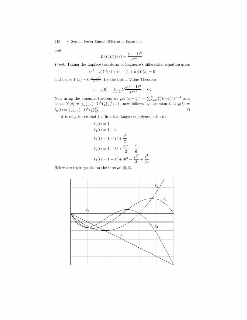
248 6 Second Order Linear Differential Equations
and
L`n(t) (s) =(s− 1)n
sn+1.
Proof. Taking the Laplace transform of Laguerre’s differential equation gives
(s2 − s)Y ′(s) + (s− (1 + n))Y (s) = 0
and hence Y (s) = C (s−1)n
sn+1 . By the Initial Value Theorem
1 = y(0) = lims→∞
Cs(s− 1)n
sn+1= C.
Now using the binomial theorem we get (s − 1)n =∑n
k=0
(
nk
)
(−1)ksn−k andhence Y (s) =
∑nk=0(−1)k
(
nk
)
1sk+1 . It now follows by inversion that y(t) =
`n(t) =∑n
k=0(−1)k(
nk
)
tk
k! . utIt is easy to see that the first five Laguerre polynomials are:
`0(t) = 1
`1(t) = 1− t
`2(t) = 1− 2t+t2
2
`3(t) = 1− 3t+3t2
2− t3
6
`4(t) = 1− 4t+ 3t2 − 2t3
3+t4
24.
Below are their graphs on the interval [0, 6].
`
`1
`2
`3
`4
6.4 Laplace Transform Methods 249
Define the following differential operators
E = 2tD2 + (2 − 2t)D− 1
E+ = tD2 + (1− 2t)D + (t− 1)
E− = tD2 + D.
Theorem 11. We have the following differential relationships amongst theLaguerre polynomials.
1. E`n = −(2n+ 1)`n2. E+`n = −(n+ 1)`n+1
3. E−`n = −n`n−1.
Proof.1. Let An = tD2+(1−t)D+n be Laguerre’s differential equation. Then from
the defining equation of the Laguerre polynomial `n we have An`n = 0.Multiply this equation by 2 and add −(1+2n)`n to both sides. This givesE`n = −(2n+ 1)`n
2. A simple observation gives E+ = An − tD − (1 − t− n). Since An`n = 0it is enough to verify that t`′n + (1− t− n)`n = (n+ 1)`n+ 1. This we doin transform space. Let Ln = L`n .Lt`′n + (1− t− n)`n (s) = −(sLn(s)− `n(0))′ + (1 − n)Ln(s) + L′
n(s)
= −(Ln + sL′n) + (1 − n)Ln + L′
n
= −(s− 1)L′n − nLn
=−(s− 1)n
sn+2(ns− (n+ 1)(s− 1)− ns)
= (n+ 1)L`n+1 (s).3. This equation is proved in a similar manner as above. We leave the details
to the exercises. J
For a differential operator A let A2y = A(Ay), A3y = A(A(Ay)), etc. It iseasy to verify by induction and the use of Theorem 11 that
(−1)n
n!En
+` = `n.
The operator E+ is called a creation operator since successive applicationsto ` creates all the other Laguerre polynomials. In a similar way it is easy toverify that
Em− `n = 0,
for all m > n. The operator E− is called an annihilation operator.
Exercises
250 6 Second Order Linear Differential Equations
1–4. For each of the following functionsshow that Theorem 6 applies and use itto find its Laplace transform.
1.ebt − eat
t
2. 2cos bt − cos at
t
3. 2cos bt − cos bt
t2
4.sin at
t
5–13. Use the Laplace transform tofind solutions to each of the following dif-ferential equations.
5. (t − 1)y′′ − ty′ + y = 0
6. ty′′ + (t − 1)y′ − y = 0
7. ty′′ + (1 + t)y′ + y = 0
8. ty′′ + (2 + 4t)y′ + (4 + 4t)y = 0
9. ty′′ − 2y′ + ty = 0
10. (t − 2)y′′ − (t − 1)t′ + y = 0
11. ty′′ + (2 + 2t)y′ + (2 + t)y = 0
12. ty′′ − 4y′ + ty = 0, assume y(0) = 0.
13. (1 + t)y′′ + (1 + 2t)y′ + ty = 0
14–18. Use the Laplace transform tofind solutions to each of the following dif-ferential equations. Use the results of Ex-ercises 1 to 4 or Table ??
14. −ty′′ + (t − 2)y′ + y = 0
15. −ty′′ − 2y′ + ty = 0
16. ty′′ + (2 − 5t)y′ + (6t − 5)y = 0
17. ty′′ + 2y′ + 9ty′ = 0
18. ty′′ + (2 + t)y′ + y = 0
19–28. Laguerre polynomials: Eachof these problems develops further prop-erties of the Laguerre polynomials.
19. The Laguerre polynomial of ordern can be defined in another way:`n(t) = 1
n!et dn
dtn (e−ttn). Show thatthis definition is consistent with thedefinition in the text.
20. Verify Equation (3) in Theorem 11:
E−`n = −n`n−1.
21. The Lie bracket [A, B] of two dif-ferential operators A and B is de-fined by
[A, B] = AB − BA.
Show the following:• [E, E+] = −2E+
• [E, E−] = 2E−
• [E+, E−] = E.
22. Show that the Laplace transform of`n(at), a ∈ R, is (s−a)n
sn+1 .
23. Verify that
n k=0 n
kak`k(t)(1 − a)n−k = `n(at).
24. Show that t
0
`n(x) dx = `n(t) − `n(t).
25. Verify the following recursion for-mula:
`n+1(t) =1
n + 1((2n + 1 − t)`n(t) − n`n−1(t)) .
26. Show that t
0
`n(x)`m(t−x)dx = `m+n(t)−`m+n+1(t).
27. Show that ∞
t
e−x`n(x) dx = e−t (`n(t) − `n−1(t)) .
28.
6.5 Reduction of Order 251
29–33. Functions of Exponentialtype: Verify the following claims.29. Show that the sum of two functions
of exponential type is of exponentialtype.
30. Show that the product of two expo-nential type functions is of exponen-tial type.
31. Show that any bounded continuousfunction on [0,∞) is of exponentialtype.
32. Show that if f is of exponential typethen any antiderivative is also of ex-ponential type.
33. Let y(t) = sin(et2). Why is y(t)of exponential type? Compute y′(t)and show that it is not of exponen-tial type. The moral: The derivativeof a function of exponential type isnot necessarily of exponential type.
6.5 Reduction of Order
It is a remarkable feature of linear differential equations that one nonzerohomogeneous solution can be used to obtain a second independent solution.Suppose L = a2(t)D
2 + a1(t)D + a0(t) and suppose y1(t) is a known nonzerosolution . Let
y2(t) = u(t)y1(t), (1)
where u(t) will be determined by substituting y2 into Ly = 0. This imposesconditions on u that are, in principle, solvable and hence will lead to a formulafor y2. The product rule for differentiation gives
y′2 = u′y1 + uy′1and y′′2 = u′′y1 + 2u′y′1 + uy′′1 .
Substituting these equations into Ly2 gives
Ly2 = a2y′′2 + a1y
′2 + a0y2
= a2(u′′y1 + 2u′y′1 + uy′′1 ) + a1(u
′y1 + uy′1) + a0uy1
= u′′a2y1 + 2u′a2y′1 + u′a1y1 + u(a2y
′′1 + a1y
′1 + a0y1)
= u′′a2y1 + u′(2a2y′1 + a1y1).
In the third line above the coefficient of u is zero because y1 is assumed to bea solution to Ly = 0. The equation Ly2 = 0 implies
u′′a2y1 + u′(2a2y′1 + a1y1) = 0, (2)
another second order differential equation in u. One obvious solution to Equa-tion 2 is u(t) a constant, implying y2 is a multiple of y1. To find anotherindependent solution we use the substitution v = u′ to get
252 6 Second Order Linear Differential Equations
v′a2y1 + v(2a2y′1 + a1y1) = 0,
a first order separable differential equation in v. This substitution gives thisprocedure its name: reduction of order. It is now straightforward to solvefor v. In fact, separating variables gives
v′
v=−2y′1y1− a1
a2.
From this we get
v =1
y21
e− a1/a2 .
Since v = u′ we integrate v to get
u =
∫
1
y21
e− a1/a2 , (3)
which is independent of the constant solution. Substituting Equation 3 intoEquation 1 then gives a new solution independent of y1. Admittedly, Equa-tion 3 is difficult to remember and not very enlightening. In the exercises werecommend following the procedure we have outlined above. This is what weshall do in the examples to follow.
Example 1. The function y1(t) = et is a solution to
(t− 1)y′′ − ty′ + y = 0.
Use reduction of order to find another independent solution and write downthe general solution.
I Solution. Let y2(t) = u(t)et. Then
y′2(t) = u′(t)et + u(t)et
y′′2 (t) = u′′(t)et + 2u′(t)et + u(t)et.
Substitution into the differential equation (t− 1)y′′ − ty′ + y = 0 gives
(t− 1)(u′′(t)et + 2u′(t)et + u(t)et)− t(u′(t)et + u(t)et) + u(t)et = 0
which simplifies to(t− 1)u′′ + (t− 2)u′ = 0.
Let v = u′. Then we get (t− 1)v′ + (t− 2)v = 0. Separating variables gives
v′
v=−(t− 2)
t− 1= −1 +
1
t− 1
with solution v = e−1(t − 1). Integration by parts gives u(t) =∫
v(t) dt =−te−t. Substitution gives
6.5 Reduction of Order 253
y2(t) = u(t)et = −te−tet = −t.It is easy to verify that this is indeed a solution. Since our equation is homoge-neous we know −y2(t) = t is also a solution. Clearly t and et are independent.By Theorem 4 the general solution is
y(t) = c1t+ c2et.
J
Example 2. In Example 6.4.9 we showed that y1 = sin tt is a solution to
ty′′ + 2y′ + ty = 0.
Use reduction of order to find a second independent solution and write downthe general solution.
I Solution. Let y2(t) = u(t) sin tt . Then
y′2(t) = u′(t)sin t
t+ u(t)
t cos t− sin t
t2
y′′2 (t) = u′′(t)sin t
t+ 2u′(t)
t cos t− sin t
t2+ u(t)
−t2 sin t− 2t cos t+ 2 sin t
t3.
We next substitute y2 into ty′′ + wy′ + ty = 0 and simplify to get
u′′(t) sin t+ 2u′(t) cos t = 0.
Let v = u′. Then we get v′(t) sin t+ 2v(t) cos t = 0. Separating variables gives
v′
v=−2 cos t
sin t
with solutionv(t) = csc2(t).
Integration gives u(t) =∫
v(t) dt = − cot(t) and hence
y2(t) = − cot tsin t
t=− cos t
t.
By Theorem 6.2.4, the general solution can be written as
c1sin t
t+ c2
cos t
t.
Compare this result with Examples 6.1.4 and 6.4.9. J
We remark that the constant of integration in the computation of u waschosen to be 0 in both examples. There is no loss in this for if a nonzeroconstant, c say, is chosen then y2 = uy1 + cy1. But cy1 is already known to bea homogeneous solution. We gain nothing by including it in y2.
Exercises
254 6 Second Order Linear Differential Equations
1–15. For each differential equation usethe given solution to find a second in-dependent solution and write down thegeneral solution.
1. t2y′′ − 3ty′ + 4y = 0 y1(t) = t2
2. t2y′′ + 2ty′ − 2y = 0, y1(t) = t
3. (1 − t2)y′′ + 2y = 0 y1(t) = 1 − t2
4. (1− t2)y′′−2ty′ +2y = 0, y1(t) = t
5. 4t2y′′ + y = 0, y1(t) =√
t
6. t2y′′ + 2ty′ = 0, y1(t) = t
7. t2y′′ − t(t + 2)y′ + (t + 2)y = 0,y1(t) = t
8. t2y′′ − 4ty′ + (t2 + 6)y = 0, y1(t) =t2 cos t
9. ty′′ − y′ + 4t3y = 0, y1(t) = sin t2
10. ty′′ − 2(t + 1) + 4y = 0, y1(t) = e2t
11. ty′′ − 2(sec2 t) y = 0, y1(t) = tan t
12. ty′′ + (t− 1)y′ − y = 0, y1(t) = e−t
13. y′′−(tan t)y′−(sec2 t)y = 0, y1(t) =tan t
14. (1+ t2)y′′−2ty′ +2y = 0, y1(t) = t
15. t2y′′ − 2ty′ + (t2 + 2)y = 0, y1(t) =t cos t
6.6 Variation of Parameters
Let L be a second order linear differential operator. In this section we addressthe issue of finding a particular solution to a nonhomogeneous linear differ-ential equation L(y) = f , where f is continuous on some interval I. It is apleasant feature of linear differential equations that the homogeneous solu-tions can be used decisively to find a particular solution. The procedure weuse is called variation of parameters and, as you shall see, is akin to themethod of reduction of order.
Suppose, in particular, that L = D2 + a1(t)D + a0(t), i.e. we will assumethat the leading coefficient function is 1 and it is important to rememberthat this assumption is essential for the method we develop below. Supposey1, y2 is a fundamental set for L(y) = 0. We know then that all solutionsof the homogeneous equation L(y) = 0 are of the form c1y1 + c2y2. To finda particular solution yp to L(y) = f the method of variation of parametersmakes two assumptions. First, the parameters c1 and c2 are allowed to vary(hence the name). We thus replace the constants c1 and c2 by functions u1(t)and u2(t), and assume that the particular solution yp, takes the form
yp(t) = u1(t)y1(t) + u2(t)y2(t). (1)
The second assumption is
u′1(t)y1(t) + u′2(t)y2(t) = 0. (2)
What’s remarkable is that these two assumptions consistently lead to explicitformulas for u1(t) and u2(t) and hence a formula for yp.
6.6 Variation of Parameters 255
To simplify notation in the calculations that follow we will drop the ‘t’in expression like u1(t), etc. Before substituting yp into L(y) = f we firstcalculate y′p and y′′p .
y′p = u′1y1 + u1y′1 + u′2y2 + u2y
′2
= u1y′1 + u2y
′2 (by Equation 2).
Now for the second derivative
y′′p = u′1y′1 + u1y
′′1 + u′2y
′2 + u2y
′′2 .
We now substitute yp into L(y).
L(yp) = y′′p + a1y′p + a0yp
= u′1y′1 + u1y
′′1 + u′2y
′2 + u2y
′′2
+a1(u1y′1 + u2y
′2)
+a0(u1y1 + u2y2)
= u′1y′1 + u′2y
′2 + u1(y
′′1 + a1y
′1 + a0y1) + u2(y
′′2 + a1y
′2 + a0y2)
= u′1y′1 + u′2y
′2.
In the second to the last equation the coefficients of u1 and u2 are zero becausey1 and y2 are assumed to be homogeneous solutions. The second assumption,Equation 2 and the equation L(yp) = f now lead to the following system:
u′1y1 + u′2y2 = 0
u′1y′1 + u′2y
′2 = f
which can be rewritten in matrix form as[
y1 y2y′1 y
′2
] [
u′1u′2
]
=
[
0f
]
. (3)
The left most matrix in Equation (3) is none other than the Wronskian matrix,W (y1, y2), which has a nonzero determinant because y1, y2 is a fundamentalset (c.f. Theorem 6.2.4 and Proposition 6.2.6). By Cramer’s rule, we can solvefor u′1 and u′2. We obtain
u′1 =−y2f
w(y1, y2)
u′2 =y1f
w(y1, y2).
We now obtain an explicit formula for a particular solution:
yp(t) = u1y1 + u2y2
=(
∫ −y2fw(y1, y2)
)
y1 +(
∫
y1f
w(y1, y2)
)
y2.
The following theorem consolidates these results with Theorem 6.1.6.
256 6 Second Order Linear Differential Equations
Theorem 1. Let L = D2 + a1(t)D+ a0(t), where a1(t) and a0(t) are contin-uous on an interval I. Suppose y1, y2 is a fundamental set of solutions forL(y) = 0. If f is continuous on I then a particular solution, yp, to L(y) = fis given by the formula
yp =(
∫ −y2fw(y1, y2)
)
y1 +(
∫
y1f
w(y1, y2)
)
y2. (4)
Furthermore, the solution set to L(y) = f becomes
yp + c1y1 + c2y2 : c1, c2 ∈ R .
Remark 2. Equation (4), which gives an explicit formula for a particularsolution, is too complicated to memorize and we do not recommend studentsto do this. Rather the point of variation of parameters is the method thatleads to Equation (4) and our recommended starting point is Equation (3).You will see such matrix equations as we proceed in the text.
We will illustrate the method of variation of parameters with two examples.
Example 3. Find the general solution to the following equation:
t2y′′ − 2y = t2 ln t.
I Solution. In standard form this becomes
y′′ − 2
t2y = ln t.
The associated homogeneous equation is y′′ − (2/t2)y = 0 or, equivalently,t2y′′ − 2y = 0 and is a Cauchy-Euler equation. The indicial polynomial isq(s) = s2 − s − 2 = (s − 2)(s + 1), which has 2 and −1 as roots. Thus
t−1, t2
is a fundamental set to the homogeneous equation y′′− (2/t2)y = 0,by Theorem 4 of Section 6.3. Let yp = t−1u1(t) + t2u2(t). Our starting pointis the matrix equation
[
t−1 t2
−t−2 2t
] [
u′1u′2
]
=
[
0ln t
]
which is equivalent to the system
t−1u′1 + t2u′2 = 0−t−2u′1 + 2tu′2 = ln t.
Multiplying the bottom equation by t and then adding the equations togethergives 3t2u′2 = t ln t and hence
u′2 =1
3tln t.
6.6 Variation of Parameters 257
Substituting u′2 into the first equation and solving for u′1 gives
u′1 = − t2
3ln t.
Integration by parts leads to
u1 = −1
3(t3
3ln t− t3
9)
and a simple substitution gives
u2 =1
6(ln t)2.
We substitute u1 and u2 into Equation (1) to get
yp(t) = −1
3(t3
3ln t− t3
9)t−1 +
1
6(ln t)2t2 =
t2
54(9(ln t)2 − 6 ln t+ 2).
It follows that the solution set is
t2
54(9(ln t)2 − 6 ln t+ 2) + c1t
−1 + c2t2 : c1, c2 ∈ R
.
J
Example 4. Find the general solution to
ty′′ + 2y′ + ty = 1.
Use the results of Example 6.5.2.
I Solution. Example 6.4.2 showed that
y1(t) =sin t
tand y2(t) =
cos t
t
are homogeneous solutions to ty′′+2y′+ty = 0. Let yp = sin tt u1(t)+
cos tt u2(t).
Then[
sin tt
cos tt
t cos t−sin tt2
−t sin t−cos tt2
][
u′1(t)
u′2(t)
]
=
[
01t
]
.
(We get 1/t in the last matrix because the differential equation in standardform is y′′ +(2/t)y′+y = 1/t.) From the matrix equation we get the followingsystem
sin t
tu′1(t) +
cos t
tu′2(t) = 0
t cos t− sin t
t2u′1(t) +
−t sin t− cos t
t2u′2(t) =
1
t.
258 6 Second Order Linear Differential Equations
The first equation gives
u′1(t) = −(cot t)u′2(t).
If we multiply the first equation by t, the second equation by t2, and then addwe get
(cos t)u′1(t) − (sin t)u′2(t) = 1.
Substituting in u′1(t) and solving for u′2(t) gives u′2(t) = − sin t and thusu′1(t) = cos t. Integration gives
u1(t) = sin t
u2(t) = cos t.
We now substitute these functions into yp to get
yp(t) =sin t
tsin t+
cos t
tcos t
=sin2 t+ cos2 t
t
=1
t.
The general solution is
y(t) =1
t+ c1
sin t
t+ c2
cos t
t.
J
Exercises
1–5. Use Variation of Parameters tofind a particular solution and then writedown the general solution. Next solveeach using the method of undeterminedcoefficients or the incomplete partialfraction method.
1. y′′ + y = sin t
2. y′′ − 4y = e2t
3. y′′ − 2y′ + 5y = et
4. y′′ + 3y′ = e−3t
5. y′′ − 3y′ + 2y = e3t
6–16. Use Variation of Parameters tofind a particular solution and then writedown the general solution. In some exer-cises a fundamental set y1, y2 is given.
6. y′′ + y = tan t
7. y′′ − 2y′ + y =et
t
8. y′′ + y = sec t
9. t2y′′ − 2ty′ + 2y = t4
6.6 Variation of Parameters 259
10. ty′′ − y′ = 3t2 − 1 y1(t) = 1 andy2(t) = t2
11. t2y′′ − ty′ + y = t
12. y′′ − 4y′ + 4y = e2t
t2+1
13. y′′ − (tan t)y′ − (sec2 t)y = ty1(t) = tan t and y2(t) = sec t
14. ty′′ + (t− 1)y′ − y = t2e−t y1(t) =t − 1 and y2(t) = e−t
15. ty′′ − y′ + 4t3y = 4t5 y1 = cos t2
and y2(t) = sin t2
16. y′′ − y = 11+e−t
17. Show that the constants of integra-tion in the formula for yp in Theorem1 can be chosen so that a particularsolution can be written in the form:
yp = t
0
y1(x) y2(x)y1(t) y2(t)y1(x) y2(x)y′2(x) y′
2(x)f(x)dx
18–21. For each problem below use theresult of Problem 17 to obtain a particu-lar solution to the given differential equa-tion in the form given. Solve the differen-tial equation using the Laplace transformmethod and compare.
18. y′′ + a2y = f(t) yp(t) = 1af(t) ∗
sin at
19. y′′ − a2y = f(t) yp(t) = 1af(t) ∗
sinh at
20. y′′ − 2ay′ + a2y = f(t) yp(t) =1af(t) ∗ te−at
21. y′′ − (a + b)y′ + aby = f(t), a 6=b yp(t) = 1
b−af(t) ∗ (ebt − eat)

7
Power Series Methods
Thus far in our study of linear differential equations we have imposed severerestrictions on the coefficient functions in order to find solution methods. Twospecial classes of note are the constant coefficient and Cauchy-Euler differen-tial equations. The Laplace transform method was also useful in solving somedifferential equations where the coefficients were linear. Outside of specialcases such as these, linear second order differential equations with variablecoefficients can be very difficult to solve.
In this chapter we introduce the use of power series in solving differentialequations. Here’s the main idea. Suppose a second order differential equation
a2(t)y′′ + a1(t)y
′ + a0(t)y = f(t)
is given. Under the right conditions on the coefficient functions a solution canbe expressed in terms of a power series which takes the form
y(t) =
∞∑
n=0
cn(t− t0)n,
for some fixed t0. Substituting the power series into the differential equationgives relationships amongst the coefficients cn∞n=0, which when solved givesa power series solution. This technique is called the power series method.While we may not enjoy a closed form solution, as in the special cases thusfar considered, power series methods imposes the least restrictions on thecoefficient functions.
7.1 A Review of Power Series
We begin with a review of the main properties of power series that are usuallylearned in a first year calculus course.
262 7 Power Series Methods
Definitions and convergence
A power series centered at t0 in the variable t is a series of the form
∞∑
n=0
cn(t− t0)n = c0 + c1(t− t0) + c2(t− t0)2 + · · · . (1)
The center of the power series is t0 and the coefficients are the constantscn∞n=0. Frequently we will simply refer to Equation (1) as a power series.Let I be the set of real numbers where the series converges. Obviously, t0 is inI, so I is nonempty. It turns out that I is an interval and is called the intervalof convergence. It contains an open interval of the form (t0−R, t0 +R) andpossibly one or both of the endpoints. The number R is called the radius ofconvergence and can frequently be determined by the ratio test.
The Ratio Test for Power Series Let∑∞
n=0 cn(t− t0)n be a given power
series and suppose L = limn→∞∣
∣
∣
cn+1
cn
∣
∣
∣. Define R in the following way:
R = 0 if L =∞R =∞ if L = 0.
R = 1L if 0 < L <∞
Then
i. The power series converges only at t = t0 if R = 0.
ii. The power series converges absolutely for all t ∈ R if R =∞.
iii. The power series converges absolutely when |t− t0| < R and diverges when|t− t0| > R if 0 < R <∞.
If R = 0 then I is the degenerate interval [t0, t0] and if R = ∞ then I =(−∞,∞). If 0 < R < ∞ then I is the interval (t0 − R, t0 + R) and possiblythe endpoints, t0−R and t0 +R, which one must check separately using othertests of convergence.
Recall that absolute convergence means that∑∞
n=0 |cn(t− t0)n| con-verges and implies the original series converges. One of the important advan-tages absolute convergence gives us is that we can add up the terms in a seriesin any order we please and still get the same result. For example, we can addall the even terms and then the odd terms separately. Thus
∞∑
n=0
cn(t− t0)n =∑
n odd
cn(t− t0)n +∑
n even
cn(t− t0)n
=
∞∑
n=0
c2n+1(t− t0)2n+1 +
∞∑
n=0
c2n(t− t0)2n.
7.1 A Review of Power Series 263
Example 1. Find the interval of convergence of the power series
∞∑
n=1
(t− 4)n
n2n.
I Solution. The ratio test gives∣
∣
∣
∣
cn+1
cn
∣
∣
∣
∣
=n2n
(n+ 1)2n+1=
n
2(n+ 1)→ 1
2
as n → ∞. The radius of convergence is 2. The interval of convergence has4 as the center and thus the endpoints are 2 and 6. When t = 2 the powerseries reduces to
∑∞n=1
(−1)n
n , which is the alternating harmonic series andknown to converge. When t = 6 the power series reduces to
∑∞n=0
1n , which is
the harmonic series and known to diverge. The interval of convergence is thusI = [ 2, 6).
Example 2. Find the interval of convergence of the power series
J0(t) =
∞∑
n=0
(−1)nt2n
22n(n!)2.
I Solution. Let u = t2. We apply the ratio test to∑∞
n=0(−1)nun
22n(n!)2 to get
∣
∣
∣
∣
cn+1
cn
∣
∣
∣
∣
=22n(n!)2
22(n+1)((n+ 1)!)2=
1
4(n+ 1)2→ 0
as n → ∞. It follows that R = ∞ and the series converges for all u. Hence∑∞
n=0(−1)nt2n
22n(n!)2 converges for all t and I = (−∞,∞). J
In each example the power series defines a function on its interval of con-vergence. In Example 2, the function J0(t) is known as the Bessel functionof order 0 and plays an important role in many physical problems. Moregenerally, let f(t) =
∑∞n=0 cn(t − t0)n for all t ∈ I. Then f is a function on
the interval of convergence I and Equation (1) is its power series repre-sentation. A simple example of a power series representation is a polynomialdefined on R. In this case the coefficients are all zero except for finitely many.Other well known examples from calculus are:
264 7 Power Series Methods
et =∞∑
n=0
tn
n!= 1 + t+
t2
2+t3
3!+ · · · (2)
cos t =
∞∑
n=0
(−1)nt2n
(2n)!= 1− t2
2+t4
4!− · · · (3)
sin t =∞∑
n=0
(−1)nt2n+1
(2n+ 1)!= t− t3
3!+t5
5!− · · · (4)
1
1− t =
∞∑
n=0
tn = 1 + t+ t2 + · · · (5)
ln t =
∞∑
n=1
(−1)(n+1)(t− 1)n
n!= (t− 1)− (t− 1)2
2+
(t− 1)3
3− · · · (6)
Equations 2, 3 and 4 are centered at 0 and have interval of convergence(−∞,∞). Equation 5, known as the geometric series, is centered at 0 andhas interval of convergence (−1, 1). Equation 6 is centered at 1 and has intervalof convergence (0, 2 ].
Index Shifting
In calculus, the variable x in a definite integral∫ b
af(x) dx is called a dummy
variable because the value of the integral is independent of x. Sometimes itis convenient to change the variable. For example, if we replace x by x− 1 inthe integral
∫ 2
11
x+1 dx we obtain
∫ 2
1
1
x+ 1dx =
∫ x−1=2
x−1=1
1
x− 1 + 1d(x− 1) =
∫ 3
2
1
xdx.
In like manner, the index n in a power series is referred to as a dummy variablebecause the sum is independent of n. It is also sometimes convenient to makea change of variable, which, for series is called an index shift. For example,
in the series∞∑
n=0(n+ 1)tn+1 we replace n by n− 1 to obtain
∞∑
n=0
(n+ 1)tn+1 =n−1=∞∑
n−1=0
(n− 1 + 1)tn−1+1 =∞∑
n=1
ntn.
The lower limit n = 0 is replaced by n − 1 = 0 or n = 1. The upper limitn =∞ is replace by n− 1 =∞ or n =∞. The terms (n+1)tn+1 in the seriesgo to (n− 1 + 1)tn−1+1 = ntn.
When a power series is given is such a way that the index n in the sum isthe power of (t − t0) we say the power series is written in standard form.
Thus∞∑
n=1ntn is in standard form while
∞∑
n=0(n+ 1)tn+1 is not.
7.1 A Review of Power Series 265
Example 3. Make an index shift so that the series∞∑
n=2
tn−2
n2 is expressed as
a series in standard form.
I Solution. We replace n by n+ 2 and get
∞∑
n=2
tn−2
n2=
n+2=∞∑
n+2=2
tn+2−2
(n+ 2)2=
∞∑
n=0
tn
(n+ 2)2.
J
Differentiation and Integration of Power Series
If a function can be represented by a power series then we can compute itsderivative and integral by differentiating and integrating each term in thepower series as noted in the following theorem.
Theorem 4. Suppose
f(t) =∞∑
n=0
cn(t− t0)n
is defined by a power series with radius of convergence R > 0. Then f isdifferentiable and integrable on (t0 −R, t0 +R) and
f ′(t) =
∞∑
n=1
ncn(t− t0)n−1 (7)
and∫
f(t) dt =
∞∑
n=0
cn(t− t0)n+1
n+ 1+ C. (8)
Furthermore, the radius of convergence for the power series representations off ′ and
∫
f are both R.
We note that the presence of the factor n in f ′(t) allows us to write
f ′(t) =
∞∑
n=0
ncn(t− t0)n−1
since the term at n = 0 is zero. This observation is occasionally used. Considerthe following examples.
Example 5. Find a power series representation for 1(1−t)2 in standard form.
I Solution. If f(t) = 11−t then f ′(t) = 1
(1−t)2 . If follows from Theorem 4that
1
(1− t)2 =d
dt
∞∑
n=0
tn =∞∑
n=1
ntn−1 =∞∑
n=0
(n+ 1)tn.
J
266 7 Power Series Methods
Example 6. Find the power series representation for ln(1 − t) in standardform.
I Solution. For t ∈ (−1, 1), ln(1− t) = −∫
11−t + C. Thus
ln(1− t) = C −∫ ∞∑
n=0
tn dt = C −∞∑
n=0
tn+1
n+ 1= C −
∞∑
n=1
tn
n.
Evaluating both side at t = 0 gives C = 0. It follows that
ln(1− t) = −∞∑
n=1
tn
n.
J
The algebra of power series
Suppose f(t) =∑∞
n=0 an(t−t0)n and g(t) =∑∞
n=0 bn(t−t0)n are power seriesrepresentation of f and g and converge on the interval (t0 − R, t0 + R) forsome R > 0. Then
f(t) = g(t) if and only if an = bn,
for all n = 1, 2, 3, . . . . Let c ∈ R. Then the power series representation of f±g,cf , fg, and f/g are given by
f(t)± g(t) =
∞∑
n=0
(an ± bn)(t− t0)n (9)
cf(t) =
∞∑
n=0
can(t− t0)n (10)
f(t)g(t) =
∞∑
n=0
cn(t− t0)n where cn = a0bn + a1bn−1 + · · ·+ anb0 (11)
andf(t)
g(t)=
∞∑
n=0
dn(t− t0)n, g(a) 6= 0, (12)
where each dn is determined by the equation f(t) = g(t)∑∞
n=0 dn(t− t0)n. InEquations 9, 10, and 11, the series converges on the interval (t0 −R, t0 +R).For division of power series, Equation 12, the radius of convergence is positivebut may not be as large as R.
Example 7. Compute the power series representations of
cosh t =et + e−t
2and sinh t =
et − e−t
2.
7.1 A Review of Power Series 267
I Solution. We write out the terms in each series, et and e−t, and get
et = 1 + t+t2
2!+t3
3!+t4
4!+ · · ·
e−t = 1− t+ t2
2!− t3
3!+t4
4!− · · ·
et + e−t = 2 + 2t2
2!+ 2
t4
4!+ · · ·
et − e−t = 2t+ 2t3
3!+ 2
t5
5!+ · · ·
It follows that
cosh t =
∞∑
n=0
t2n
(2n)!and sinh t =
∞∑
n=0
t2n+1
(2n+ 1)!.
J
Example 8. Let y(t) =∞∑
n=0cnt
n. Compute
(1 + t2)y′′ + 4ty′ + 2y
as a power series.
I Solution. We differentiate y twice to get
y′(t) =
∞∑
n=1
cnntn−1 and y′′(t) =
∞∑
n=2
cnn(n− 1)tn−2.
In the following calculations we shift indices as necessary to obtain series instandard form.
t2y′′ =∞∑
n=2
cnn(n− 1)tn =∞∑
n=0
cnn(n− 1)tn
y′′ =
∞∑
n=2
cnn(n− 1)tn−2 =
∞∑
n=0
cn+2(n+ 2)(n+ 1)tn
4ty′ =
∞∑
n=1
4cnntn =
∞∑
n=0
4cnntn
2y =
∞∑
n=0
2cntn
Notice that the presence of the factors n and n − 1 in the first series allowsus to write it with a starting point n = 0 instead of n = 2; similarly for thethird series. Adding these results and simplifying gives
268 7 Power Series Methods
(1 + t2)y′′ + 4ty′ + 2y =∞∑
n=0
((cn+2 + cn)(n+ 2)(n+ 1)) tn.
J
A function f is said to be an odd function if f(−t) = −f(t) and even iff(−t) = f(t). If f is odd and has a power series representation with center 0then all coefficients of even powers of t are zero. Similarly, if f is even thenall the coefficients of odd powers are zero. Thus f has the following form:
f(t) = a0 + a2t2 + a4t
4 + . . . =∞∑
n=0
a2nt2n f -even
f(t) = a1t+ a3t3 + a5t
5 + . . . =∞∑
n=0a2n+1t
2n+1 f -odd.
For example, the power series representations of cos t and cosh t reflect thatthey are even and while those of sin t and sinh t reflect that they are oddfunctions.
Example 9. Compute the first four nonzero terms in the power series rep-resentation of
tanh t =sinh t
cosh t.
I Solution. Division of power series is generally complicated. To makethings a little simpler here we observe that tanh t is an odd function. Thus
its power series expansion is of the form tanh t =∞∑
n=1d2n+1t
2n+1 and satisfies
sinh t = cosh t∞∑
n=0d2n+1t
2n+1. By Example 7 this means
(
t+t3
3!+t5
5!+ · · ·
)
=
(
1 +t2
2!+t4
4!+ · · ·
)
(
d1t+ d3t3 + d5t
5 + · · ·)
=
(
d1t+ (d3 +d1
2!)t3 + (d5 +
d3
2!+d1
4!)t5 + · · ·
)
.
We now equate coefficients to get the following sequence of equations:
d1 = 1
d3 +d1
2!=
1
3!
d5 +d3
2!+d1
4!=
1
5!
d7 +d5
2!+d3
4!+d1
6!=
1
7!...
7.1 A Review of Power Series 269
Recursively solving these equations gives d1 = 1, d3 = −13 , d5 = 2
15 , andd7 = −17
315 . The first four nonzero terms in the power series expansion fortanh t is thus
tanh t = t− 1
3t3 +
2
15t5 − 17
315t7 + · · · .
J
Identifying Power Series
Given a power series, with positive radius of convergence, it is sometimespossible to identify it with a known function. When we can do this we willsay that it is written in closed form. Usually, such identification come byusing a combination of differentiation, integration, or the algebraic propertiesof power series discussed above. Consider the following examples.
Example 10. Write the power series
∞∑
n=0
t2n+1
n!
in closed form.
I Solution. Observe that we can factor out t and associate the term t2 toget
∞∑
n=0
t2n+1
n!= t
∞∑
n=0
(t2)n
n!= tet2 ,
from Equation 2. J
Example 11. Write the power series
∞∑
n=1
n(−1)nt2n
in closed form.
I Solution. Let z(t) =∞∑
n=1n(−1)nt2n. Then dividing both sides by t gives
z(t)
t=
∞∑
n=1
n(−1)nt2n−1.
Integration will now simplify the sum:
270 7 Power Series Methods
∫
z(t)
tdt =
∞∑
n=1
∫
n(−1)nt2n−1 dt
=
∞∑
n=1
(−1)n t2n
2
=1
2
∞∑
n=1
(−t2)n
=1
2
(
1
1 + t2− 1
)
+ c,
where the last line is obtained from the geometric series by adding and sub-tracting the n = 0 term and c is a constant of integration. We now differentiatethis equation to get
z(t)
t=
1
2
d
dt
(
1
1 + t2− 1
)
=−t
(1 + t2)2.
It follows now that
z(t) =−t2
(1 + t2)2.
It is straightforward to check that the radius of convergence is 1 so we get theequality
−t2(1 + t2)2
=
∞∑
n=1
n(−1)nt2n,
on the interval (−1, 1). J
Taylor Series
Suppose f(t) =∑∞
n=0 cn(t− t0)n, with positive radius of converge. Theorem4 implies that the derivatives, f (n), exist for all n = 0, 1, . . .. Furthermore, it
is easy to check that f (n)(t0) = n!cn and thus cn = f(n)(t0)n! . Therefore, if f is
represented by a power series then it must be that
f(t) =
∞∑
n=0
f (n)(t0)
n!(t− t0)n. (13)
This series is called the Taylor Series of f centered at t0.Now let’s suppose that f is a function on some domain D and we wish to
find a power series representation centered at t0 ∈ D. By what we have justargued f will have to be given by its Taylor Series, which, of course, meansthat that all higher order derivatives of f at t0 must exist. However, it can
7.1 A Review of Power Series 271
happen that the Taylor series may not converge to f on any interval containingt0 (See Problems 28–32 where such an example is considered). When Equation13 is valid on an open interval containing t0 we call f analytic at t0. Theproperties of power series listed above shows that the sum, difference, scalarmultiple and product of analytic functions is again analytic. The quotient ofanalytic functions is likewise analytic at points where the denominator is notzero. Derivatives and integrals of analytic functions are again analytic.
Example 12. Verify that the Taylor series of sin t centered at 0 is that givenin Equation 4.
I Solution. The first four derivatives of sin t and their values at 0 are asfollows:
order n sin(n)(t) sin(n)(0)
n = 0 sin t 0n = 1 cos t 1n = 2 − sin t 0n = 3 − cos t −1n = 4 sin t 0
The sequence 0, 1, 0,−1 thereafter repeats. Hence, the Taylor series of sin t is
0 + 1t+ 0t2
2!− t3
3!+ 0
t4
4!+ 1
t5
5!+ · · · =
∞∑
n=0
t2n+1
(2n+ 1)!,
as in Equation 4. J
Given a function f , it can sometimes be difficult to compute the Taylorseries by computing f (n)(t0) for all n = 0, 1, . . .. For example, compute thefirst few derivatives of tanh t, considered in Example 9, to see how complicatedthe derivatives become. Additionally, determining whether the Taylor seriesconverges to f requires some additional information, for example, the Taylorremainder theorem. We will not include this in our review. Rather we will stickto examples where we derive new power series representations from existingones as we did in Examples 5 – 9.
Rational Functions
A rational function is the quotient of two polynomials and is analytic atall points where the denominator is nonzero. Rational functions will arise inmany examples. It will be convenient to know what the radius of convergenceabout a point t0. The following theorem allows us to determine this withoutgoing through the work of determining the power series. The proof is beyondthe scope of this text.
272 7 Power Series Methods
Theorem 13. Suppose p(t)q(t) is a quotient of two polynomials p and q. Suppose
q(t0) 6= 0. Then the power series expansion for pq about t0 has radius of con-
vergence equal to the closest distance from t0 to the roots (including complexroots) of q.
Example 14. Find the radius of convergence for each rational functionabout the given point.
1. t4−t about t0 = 1
2. 1−t9−t2 about t0 = 2
3. t3
t2+1 about t0 = 2
I Solution.
1. The only root of 4 − t is 4. Its distance to t0 = 1 is 3. The radius ofconvergence is 3.
2. The roots of 9 − t2 are 3 and −3. Their distances to t0 = 2 is 1 and 5,respectively. The radius of convergence is 1.
3. The roots of t2 +1 are i and −i. Their distances to t0 = 2 are |2− i| =√
5and |2 + i| =
√5. The radius of convergence is
√5.
J
Exercises
1–9. Compute the radius of conver-gence for the given power series.
1.∞
n=0
n2(t − 2)n
2.∞
n=1
tn
n
3.∞
n=0
(t − 1)n
2nn!
4.∞
n=0
3n(t − 3)n
n + 1
5.∞
n=0
n!tn
6.∞
n=0
(−1)nt2n
(2n + 1)!
7.∞
n=0
(−1)nt2n+1
(2n)!
8.∞
n=0
nntn
n!
9.∞
n=0
n!tn
1 · 3 · 5 · · · (2n + 1)
10–17. Find the Taylor series for eachfunction with center t0 = 0.
10.1
1 + t2
11.1
t − a
12. eat
13.sin t
t
7.1 A Review of Power Series 273
14.et − 1
t
15. tan−1 t
16. ln(1 + t2)
17.
18–21. Find the first four nonzeroterms in the Taylor series with center 0for each function.18. tan t
19. sec t
Solving these equations gives
d0 = 1
d2 =1
2
d4 =5
4!
d6 =69
6!.
Thus sec t = 1 + 12t2 + 5
4!t4 + 61
6!t6 +
· · · .20. et sin t
21. et cos t
26–27. Find a closed form expressionfor each power series.22.
∞n=0(−1)n n+1
n!tn
23.
24. Redo Exercises 20 and 21 in the fol-lowing way. Recall Euler’s formulaeit = cos t + i sin t and write et cos tand et sin t as the real and imaginaryparts of eteit = e(1+i)t expanded asa power series.
25. Use the power series (with center0) for the exponential function andexpand both sides of the equationeatebt = e(a+b)t. What well-knownformula arises when the coefficientsof tn
n!are equated?
26–27. A test similar to the ratio testis the root test.
The Root Test for Power Series Let∞n=0 cn(t− t0)
n be a given power series
and suppose L = limn→∞n|cn|. Define
R in the following way:
R = 1L
if 0 < L < ∞R = 0 if L = ∞R = ∞ if L = 0.
Then
i. The power series converges only att = t0 if R = 0.
ii. The power series converges for allt ∈ R if R = ∞.
iii. The power series converges if|t − t0| < R and diverges if |t − t0| >R.
26. Use the root test to determine the
radius of convergence of∞
n=0
tn
nn .
27. Let cn = 1 if n is odd and cn = 2 ifn is even. Consider the power series∞
n=0 cntn. Show that the ratio testdoes not apply. Use the root test todetermine the radius of convergence.
28–32. In this sequence of exercises weconsider a function that is infinitely dif-ferentiable but not analytic. Let
f(t) = 0 if t ≤ 0
e−1t if t > 0
.
28. Compute f ′(t) and f ′′(t) and ob-
serve that f (n)(t) = e−1t pn( 1
t) where
pn is a polynomial, n = 1, 2. Find p1
and p2.
29. Use mathematical induction to showthat f (n)(t) = e
−1t pn( 1
t) where pn is
a polynomial.
30. Show that limt→0+
f (n)(t) = 0. To do
this let u = 1t
in f (n)(t) = e−1t pn( 1
t)
and let u → ∞. Apply L’Hospitalsrule.
31. Show that fn(0) = 0 for all n =0, 1, . . ..
32. Conclude that f is not analytic att = 0 though all derivatives at t = 0exist.
274 7 Power Series Methods
7.2 Power Series Solutions about an Ordinary Point
A point t0 is called an ordinary point of Ly = 0 if we can write the differ-ential equation in the form
y′′ + a1(t)y′ + a0(t)y = 0, (1)
where a0(t) and a1(t) are analytic at t0. If t0 is not an ordinary point we callit a singular point.
Example 1. Determine the ordinary and singular points for each of thefollowing differential equations.
1. y′′ + 1t2−9y
′ + 1t+1y = 0
2. (1− t2)y′′ − 2ty′ + n(n+ 1)y = 0, where n is an integer.3. ty′′ + sin ty′ + (et − 1)y = 0
I Solution.
1. Here a1(t) = 1t2−9 is analytic except at t = ±3. The function a0 = 1
t+1 isanalytic except at t = −1. Thus the singular points at −3, 3, and −1. Allother points are ordinary.
2. This is Legendre’s equation. In standard form we find a1(t) = −2t1−t2 and
a0(t) = n(n+1)1−t2 . They are analytic except at 1 and −1. These are the
singular points and all other points are ordinary.3. In standard form a1(t) = sin t
t and a0(t) = et−1t . Both of these are analytic
everywhere. (See Exercises 13 and 14 in Section 7.) It follows that all pointsare ordinary.
In this section we restrict our attention to ordinary points. Their impor-tance is underscored by the following theorem. It tells us that there is alwaysa power series solution about ordinary points.
Theorem 2. Suppose a0(t) and a1(t) are analytic at t0, both of which con-verge for |t− t0| < R. Then there is a unique solution y(t), analytic at t0, tothe initial value problem
y′′ + a1(t)y′ + a0(t)y = 0, y(t0) = α, y′(t0) = β. (2)
If
y(t) =
∞∑
n=0
cn(t− t0)n
then c0 = α, c1 = β, and all other ck, k = 2, 3, . . ., are determined by c0 andc1. Furthermore, the power series for y converges for |t− t0| < R.
7.2 Power Series Solutions about an Ordinary Point 275
Of course the Uniqueness and Existence Theorem, Theorem 6 of Section6.1, implies there is a unique solution. What is new here is that the solution isanalytic at t0. Since the solution is necessarily unique it is not at all surprisingthat the coefficients are determined by the initial conditions. The only hardpart about the proof, which we omit, is showing that the solution convergesfor |t− t0| < R. Let y1 be the solution with initial conditions y(t0) = 1 andy′(t0) = 0 and y2 the solution with initial condition y(t0) = 0 and y′(t0) = 1.Then it is easy to see that y1 and y2 are independent solutions and henceall solutions are of the form c1y1 + c2y2. (See the proof of Theorem 4 inSection 6.2.) The power series method refers to the use of this theoremby substituting y(t) =
∑∞n=0 cn(t− t0)n into Equation 2 and determining the
coefficients.We illustrate the use of Theorem 2 with a few examples. Let’s begin with
a familiar constant coefficient differential equation.
Example 3. Use the power series method to solve
y′′ + y = 0.
I Solution. Of course, we can solve this equation by the characteristic poly-nomial s2 + 1 to get c1 sin t+ c2 cos t. Let’s see how the power series methodgives the same answer. Since the coefficients are constant they are analyticeverywhere with infinite radius of convergence. Theorem 2 implies that thepower series solutions converge everywhere. Let y(t) =
∑∞n=0 cnt
n be a powerseries about t0 = 0. Then
y′(t) =
∞∑
n=1
cnntn−1
and y′′(t) =
∞∑
n=2
cnn(n− 1)tn−2.
An index shift, n→ n+2, gives y′′(t) =∑∞
n=0 cn+2(n+2)(n+1)tn. Therefore,the equation y′′ + y = 0 gives
∞∑
n=0
(cn + cn+2(n+ 2)(n+ 1))tn = 0,
which implies cn + cn+2(n+ 2)(n+ 1) = 0, or, equivalently,
cn+2 =−cn
(n+ 2)(n+ 1)for all n = 0, 1, . . .. (3)
Equation 3 is an example of a recurrence relation: terms of the sequenceare determined by earlier terms. Since the difference in indices between cn andcn+2 is 2 it follows that even terms are determined by previous even termsand odd terms are determined by previous odd terms. Let’s consider thesetwo cases separately.
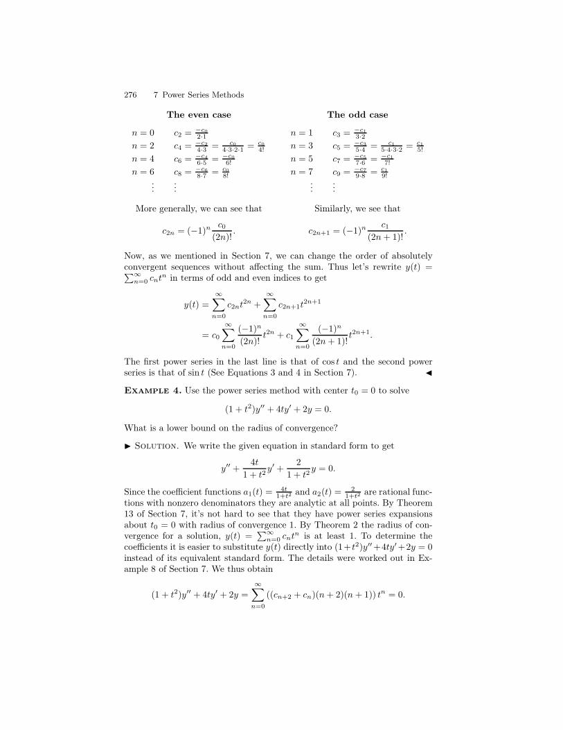
276 7 Power Series Methods
The even case
n = 0 c2 = −c0
2·1n = 2 c4 = −c2
4·3 = c0
4·3·2·1 = c0
4!
n = 4 c6 = −c4
6·5 = −c0
6!
n = 6 c8 = −c6
8·7 = c0
8!...
...
More generally, we can see that
c2n = (−1)n c0(2n)!
.
The odd case
n = 1 c3 = −c1
3·2n = 3 c5 = −c3
5·4 = c1
5·4·3·2 = c1
5!
n = 5 c7 = −c5
7·6 = −c1
7!
n = 7 c9 = −c7
9·8 = c1
9!...
...
Similarly, we see that
c2n+1 = (−1)n c1(2n+ 1)!
.
Now, as we mentioned in Section 7, we can change the order of absolutelyconvergent sequences without affecting the sum. Thus let’s rewrite y(t) =∑∞
n=0 cntn in terms of odd and even indices to get
y(t) =
∞∑
n=0
c2nt2n +
∞∑
n=0
c2n+1t2n+1
= c0
∞∑
n=0
(−1)n
(2n)!t2n + c1
∞∑
n=0
(−1)n
(2n+ 1)!t2n+1.
The first power series in the last line is that of cos t and the second powerseries is that of sin t (See Equations 3 and 4 in Section 7). J
Example 4. Use the power series method with center t0 = 0 to solve
(1 + t2)y′′ + 4ty′ + 2y = 0.
What is a lower bound on the radius of convergence?
I Solution. We write the given equation in standard form to get
y′′ +4t
1 + t2y′ +
2
1 + t2y = 0.
Since the coefficient functions a1(t) = 4t1+t2 and a2(t) = 2
1+t2 are rational func-tions with nonzero denominators they are analytic at all points. By Theorem13 of Section 7, it’s not hard to see that they have power series expansionsabout t0 = 0 with radius of convergence 1. By Theorem 2 the radius of con-vergence for a solution, y(t) =
∑∞n=0 cnt
n is at least 1. To determine thecoefficients it is easier to substitute y(t) directly into (1+ t2)y′′+4ty′+2y = 0instead of its equivalent standard form. The details were worked out in Ex-ample 8 of Section 7. We thus obtain
(1 + t2)y′′ + 4ty′ + 2y =
∞∑
n=0
((cn+2 + cn)(n+ 2)(n+ 1)) tn = 0.
7.2 Power Series Solutions about an Ordinary Point 277
From this equation we get cn+2+cn = 0 for all n = 0, 1, · · · . Again we considereven and odd cases.
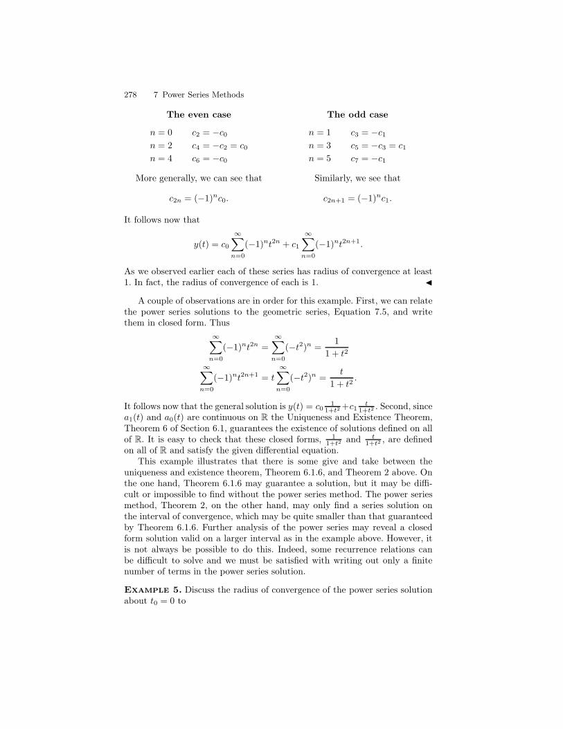
278 7 Power Series Methods
The even case
n = 0 c2 = −c0n = 2 c4 = −c2 = c0
n = 4 c6 = −c0
More generally, we can see that
c2n = (−1)nc0.
The odd case
n = 1 c3 = −c1n = 3 c5 = −c3 = c1
n = 5 c7 = −c1
Similarly, we see that
c2n+1 = (−1)nc1.
It follows now that
y(t) = c0
∞∑
n=0
(−1)nt2n + c1
∞∑
n=0
(−1)nt2n+1.
As we observed earlier each of these series has radius of convergence at least1. In fact, the radius of convergence of each is 1. J
A couple of observations are in order for this example. First, we can relatethe power series solutions to the geometric series, Equation 7.5, and writethem in closed form. Thus
∞∑
n=0
(−1)nt2n =
∞∑
n=0
(−t2)n =1
1 + t2
∞∑
n=0
(−1)nt2n+1 = t
∞∑
n=0
(−t2)n =t
1 + t2.
It follows now that the general solution is y(t) = c01
1+t2 +c1t
1+t2 . Second, sincea1(t) and a0(t) are continuous on R the Uniqueness and Existence Theorem,Theorem 6 of Section 6.1, guarantees the existence of solutions defined on allof R. It is easy to check that these closed forms, 1
1+t2 and t1+t2 , are defined
on all of R and satisfy the given differential equation.This example illustrates that there is some give and take between the
uniqueness and existence theorem, Theorem 6.1.6, and Theorem 2 above. Onthe one hand, Theorem 6.1.6 may guarantee a solution, but it may be diffi-cult or impossible to find without the power series method. The power seriesmethod, Theorem 2, on the other hand, may only find a series solution onthe interval of convergence, which may be quite smaller than that guaranteedby Theorem 6.1.6. Further analysis of the power series may reveal a closedform solution valid on a larger interval as in the example above. However, itis not always be possible to do this. Indeed, some recurrence relations canbe difficult to solve and we must be satisfied with writing out only a finitenumber of terms in the power series solution.
Example 5. Discuss the radius of convergence of the power series solutionabout t0 = 0 to
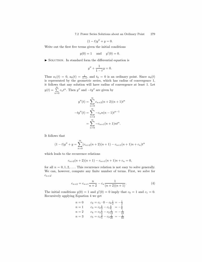
7.2 Power Series Solutions about an Ordinary Point 279
(1− t)y′′ + y = 0.
Write out the first five terms given the initial conditions
y(0) = 1 and y′(0) = 0.
I Solution. In standard form the differential equation is
y′′ +1
1− ty = 0.
Thus a1(t) = 0, a0(t) = 11−t , and t0 = 0 is an ordinary point. Since a0(t)
is represented by the geometric series, which has radius of convergence 1,it follows that any solution will have radius of convergence at least 1. Let
y(t) =∞∑
n=0
cntn. Then y′′ and −ty′′ are given by
y′′(t) =
∞∑
n=0
cn+2(n+ 2)(n+ 1)tn
−ty′′(t) =
∞∑
n=2
−cnn(n− 1)tn−1
=∞∑
n=0
−cn+1(n+ 1)ntn.
It follows that
(1 − t)y′′ + y =
∞∑
n=0
(cn+2(n+ 2)(n+ 1)− cn+1(n+ 1)n+ cn)tn
which leads to the recurrence relations
cn+2(n+ 2)(n+ 1)− cn+1(n+ 1)n+ cn = 0,
for all n = 0, 1, 2, . . . . This recurrence relation is not easy to solve generally.We can, however, compute any finite number of terms. First, we solve forcn+2:
cn+2 = cn+1n
n+ 2− cn
1
(n+ 2)(n+ 1). (4)
The initial conditions y(0) = 1 and y′(0) = 0 imply that c0 = 1 and c1 = 0.Recursively applying Equation 4 we get
n = 0 c2 = c1 · 0− c0 12 = − 1
2
n = 1 c3 = c213 − c1 1
6 = − 16
n = 2 c4 = c312 − c2 1
12 = − 124
n = 3 c5 = c435 − c3 1
20 = − 160

280 7 Power Series Methods
It now follows that the first five terms of y(t) is
y(t) = 1− 1
2t2 − 1
6t3 − 1
24t4 − 1
60t5.
J
In general, it may not be possible to find a closed form description of cn.Nevertheless, we can use the recurrence relation to find as many terms as wedesire. Although this may be tedious it may suffice to give an approximatesolution to a given differential equation.
We note that the examples we gave are power series solutions about t0 = 0.We can always reduce to this case by a substitution. To illustrate consider thedifferential equation
ty′′ − (t− 1)y′ − ty = 0. (5)
It has t0 = 1 as an ordinary point. Suppose we wish to derive a power seriessolution about t0 = 1. Let y(t) be a solution and let Y (x) = y(x + 1). ThenY ′(x) = y′(x + 1) and Y ′′(x) = y′′(x + 1). In the variable x, Equation 5becomes (x+ 1)Y ′′(x)− xY ′(x)− (x+ 1)Y (x) = 0 and x0 = 0 is an ordinary
point. We solve Y (x) =∞∑
n=0
cnxn as before. Now let x = t − 1. I.e. y(t) =
Y (t− 1) =∑∞
n=0 cn(t− 1)n is the series solution to Equation 5 about t0 = 1.
Chebyshev Polynomials
We conclude this section with the following two related problems: For a non-negative integer n expand cosnx and sinnx in terms of just cosx and sinx. Itis an easy exercise (see Exercises 13 and 14) to show that we can write cosnxas a polynomial in cosx and we can write sinnx as a product of sinx anda polynomial in cosx. More specifically, we will find polynomials Tn and Un
such that
cosnx = Tn(cosx)
sin(n+ 1)x = sinxUn(cosx).(6)
(The shift by 1 in the formula defining Un is intentional.) The polynomialsTn and Un are called the Chebyshev polynomials of the first and secondkind, respectively. They each have degree n. For example, if n = 2 we havecos 2x = cos2 x − sin2 x = 2 cos2 x − 1. Thus T2(t) = 2t2 − 1; if t = cosx wehave
cos 2x = T2(cosx).
Similarly, sin 2x = 2 sinx cosx. Thus U1(t) = 2t and
sin 2x = sinxU1(cosx).
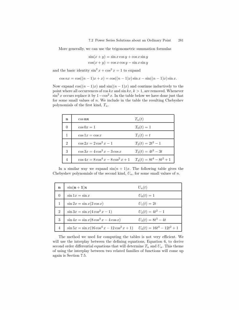
7.2 Power Series Solutions about an Ordinary Point 281
More generally, we can use the trigonometric summation formulas
sin(x+ y) = sinx cos y + cosx sin y
cos(x+ y) = cosx cos y − sinx sin y
and the basic identity sin2 x+ cos2 x = 1 to expand
cosnx = cos((n− 1)x+ x) = cos((n− 1)x) sinx− sin((n− 1)x) sinx.
Now expand cos((n− 1)x) and sin((n− 1)x) and continue inductively to thepoint where all occurrences of cos kx and sin kx, k > 1, are removed. Wheneversin2 x occurs replace it by 1−cos2 x. In the table below we have done just thatfor some small values of n. We include in the table the resulting Chebyshevpolynomials of the first kind, Tn.
n cosnx Tn(t)
0 cos 0x = 1 T0(t) = 1
1 cos 1x = cosx T1(t) = t
2 cos 2x = 2 cos2 x− 1 T2(t) = 2t2 − 1
3 cos 3x = 4 cos3 x− 3 cosx T3(t) = 4t3 − 3t
4 cos 4x = 8 cos4 x− 8 cos2 x+ 1 T4(t) = 8t4 − 8t2 + 1
In a similar way we expand sin(n + 1)x. The following table gives theChebyshev polynomials of the second kind, Un, for some small values of n.
n sin(n + 1)x Un(t)
0 sin 1x = sinx U0(t) = 1
1 sin 2x = sinx(2 cosx) U1(t) = 2t
2 sin 3x = sinx(4 cos2 x− 1) U2(t) = 4t2 − 1
3 sin 4x = sinx(8 cos3 x− 4 cosx) U3(t) = 8t3 − 4t
4 sin 5x = sinx(16 cos4 x− 12 cos2 x+ 1) U4(t) = 16t4 − 12t2 + 1
The method we used for computing the tables is not very efficient. Wewill use the interplay between the defining equations, Equation 6, to derivesecond order differential equations that will determine Tn and Un. This themeof using the interplay between two related families of functions will come upagain is Section 7.5.
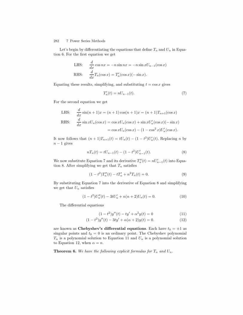
282 7 Power Series Methods
Let’s begin by differentiating the equations that define Tn and Un in Equa-tion 6. For the first equation we get
LHS:d
dxcosnx = −n sinnx = −n sinxUn−1(cosx)
RHS:d
dxTn(cos x) = T ′
n(cosx)(− sinx).
Equating these results, simplifying, and substituting t = cosx gives
T ′n(t) = nUn−1(t). (7)
For the second equation we get
LHS:d
dxsin(n+ 1)x = (n+ 1) cos(n+ 1)x = (n+ 1)Tn+1(cos x)
RHS:d
dxsinxUn(cosx) = cosxUn(cosx) + sinxU ′
n(cos x)(− sinx)
= cosxUn(cosx)− (1− cos2 x)U ′n(cos x).
It now follows that (n + 1)Tn+1(t) = tUn(t) − (1 − t2)U ′n(t). Replacing n by
n− 1 gives
nTn(t) = tUn−1(t)− (1− t2)U ′n−1(t). (8)
We now substitute Equation 7 and its derivative T ′′n (t) = nU ′
n−1(t) into Equa-tion 8. After simplifying we get that Tn satisfies
(1 − t2)T ′′n (t)− tT ′
n + n2Tn(t) = 0. (9)
By substituting Equation 7 into the derivative of Equation 8 and simplifyingwe get that Un satisfies
(1− t2)U ′′n (t)− 3tU ′
n + n(n+ 2)Un(t) = 0. (10)
The differential equations
(1− t2)y′′(t)− ty′ + α2y(t) = 0 (11)
(1− t2)y′′(t)− 3ty′ + α(α + 2)y(t) = 0. (12)
are known as Chebyshev’s differential equations. Each have t0 = ±1 assingular points and t0 = 0 is an ordinary point. The Chebyshev polynomialTn is a polynomial solution to Equation 11 and Un is a polynomial solutionto Equation 12, when α = n.
Theorem 6. We have the following explicit formulas for Tn and Un.
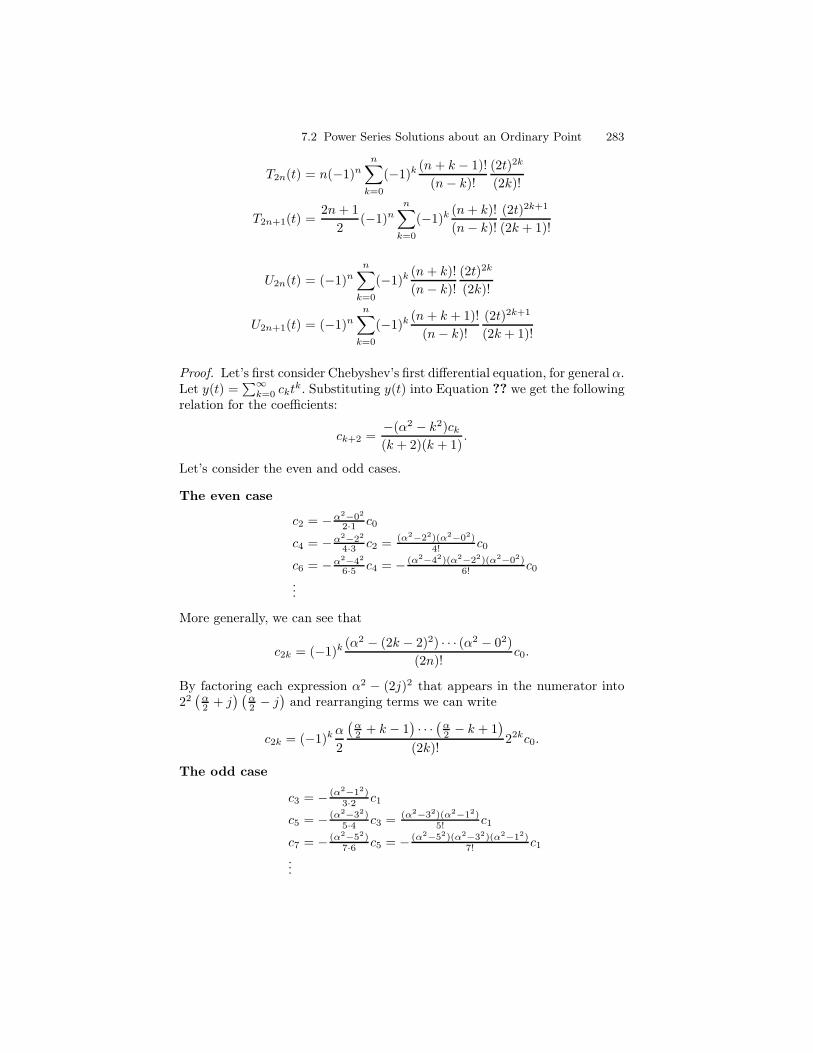
7.2 Power Series Solutions about an Ordinary Point 283
T2n(t) = n(−1)nn∑
k=0
(−1)k (n+ k − 1)!
(n− k)!(2t)2k
(2k)!
T2n+1(t) =2n+ 1
2(−1)n
n∑
k=0
(−1)k (n+ k)!
(n− k)!(2t)2k+1
(2k + 1)!
U2n(t) = (−1)nn∑
k=0
(−1)k (n+ k)!
(n− k)!(2t)2k
(2k)!
U2n+1(t) = (−1)nn∑
k=0
(−1)k (n+ k + 1)!
(n− k)!(2t)2k+1
(2k + 1)!
Proof. Let’s first consider Chebyshev’s first differential equation, for general α.Let y(t) =
∑∞k=0 ckt
k. Substituting y(t) into Equation ?? we get the followingrelation for the coefficients:
ck+2 =−(α2 − k2)ck(k + 2)(k + 1)
.
Let’s consider the even and odd cases.
The even case
c2 = −α2−02
2·1 c0
c4 = −α2−22
4·3 c2 = (α2−22)(α2−02)4! c0
c6 = −α2−42
6·5 c4 = − (α2−42)(α2−22)(α2−02)6! c0
...
More generally, we can see that
c2k = (−1)k (α2 − (2k − 2)2) · · · (α2 − 02)
(2n)!c0.
By factoring each expression α2 − (2j)2 that appears in the numerator into22(
α2 + j
) (
α2 − j
)
and rearranging terms we can write
c2k = (−1)kα
2
(
α2 + k − 1
)
· · ·(
α2 − k + 1
)
(2k)!22kc0.
The odd case
c3 = − (α2−12)3·2 c1
c5 = − (α2−32)5·4 c3 = (α2−32)(α2−12)
5! c1
c7 = − (α2−52)7·6 c5 = − (α2−52)(α2−32)(α2−12)
7! c1...
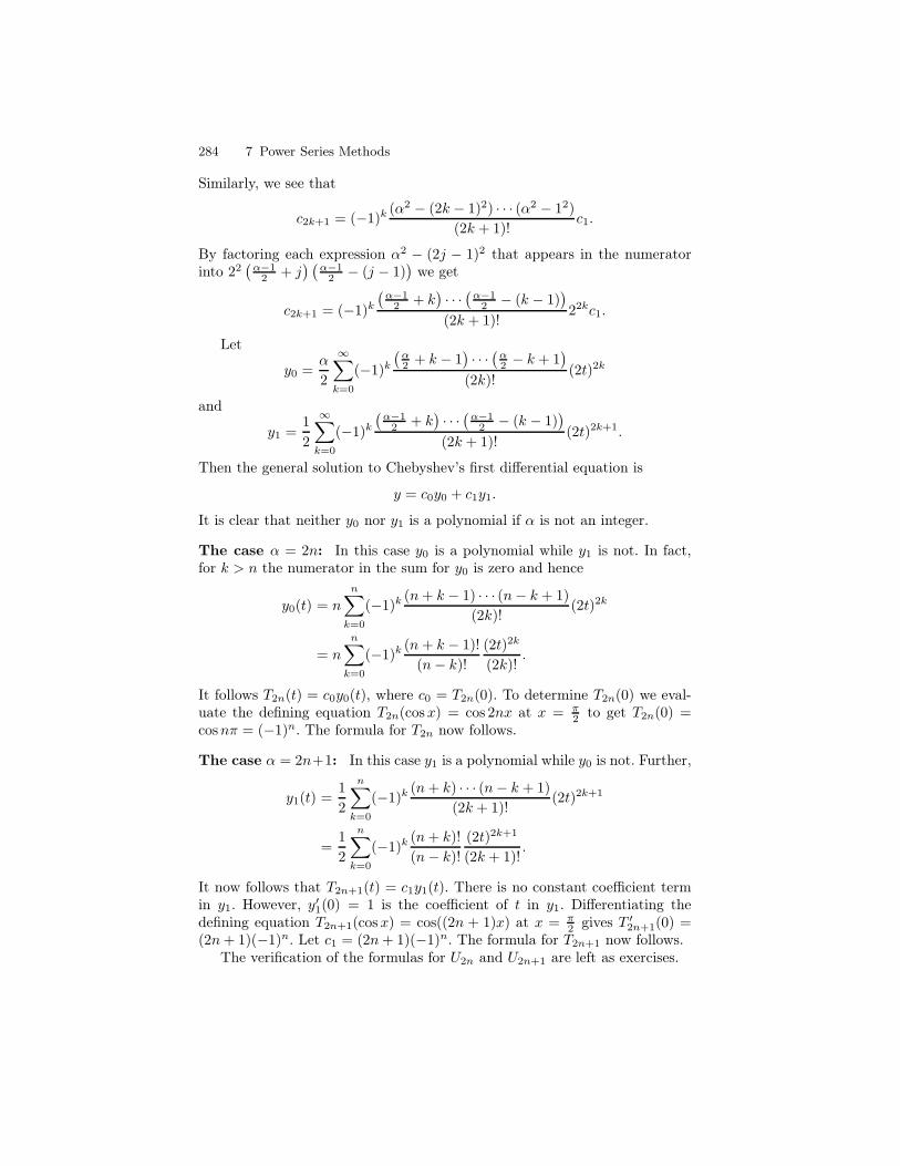
284 7 Power Series Methods
Similarly, we see that
c2k+1 = (−1)k (α2 − (2k − 1)2) · · · (α2 − 12)
(2k + 1)!c1.
By factoring each expression α2 − (2j − 1)2 that appears in the numeratorinto 22
(
α−12 + j
) (
α−12 − (j − 1)
)
we get
c2k+1 = (−1)k
(
α−12 + k
)
· · ·(
α−12 − (k − 1)
)
(2k + 1)!22kc1.
Let
y0 =α
2
∞∑
k=0
(−1)k
(
α2 + k − 1
)
· · ·(
α2 − k + 1
)
(2k)!(2t)2k
and
y1 =1
2
∞∑
k=0
(−1)k
(
α−12 + k
)
· · ·(
α−12 − (k − 1)
)
(2k + 1)!(2t)2k+1.
Then the general solution to Chebyshev’s first differential equation is
y = c0y0 + c1y1.
It is clear that neither y0 nor y1 is a polynomial if α is not an integer.
The case α = 2n: In this case y0 is a polynomial while y1 is not. In fact,for k > n the numerator in the sum for y0 is zero and hence
y0(t) = nn∑
k=0
(−1)k (n+ k − 1) · · · (n− k + 1)
(2k)!(2t)2k
= n
n∑
k=0
(−1)k (n+ k − 1)!
(n− k)!(2t)2k
(2k)!.
It follows T2n(t) = c0y0(t), where c0 = T2n(0). To determine T2n(0) we eval-uate the defining equation T2n(cosx) = cos 2nx at x = π
2 to get T2n(0) =cosnπ = (−1)n. The formula for T2n now follows.
The case α = 2n+1: In this case y1 is a polynomial while y0 is not. Further,
y1(t) =1
2
n∑
k=0
(−1)k (n+ k) · · · (n− k + 1)
(2k + 1)!(2t)2k+1
=1
2
n∑
k=0
(−1)k (n+ k)!
(n− k)!(2t)2k+1
(2k + 1)!.
It now follows that T2n+1(t) = c1y1(t). There is no constant coefficient termin y1. However, y′1(0) = 1 is the coefficient of t in y1. Differentiating thedefining equation T2n+1(cosx) = cos((2n + 1)x) at x = π
2 gives T ′2n+1(0) =
(2n+ 1)(−1)n. Let c1 = (2n+ 1)(−1)n. The formula for T2n+1 now follows.The verification of the formulas for U2n and U2n+1 are left as exercises.
7.2 Power Series Solutions about an Ordinary Point 285
Exercises
1–4. Use the power series methodabout t0 = 0 to solve the given differ-ential equation. Identify the power se-ries with known functions. Since each areconstant coefficient use the characteristicpolynomial to solve and compare.
1. y′′ − y = 0
2. y′′ − 2y′ + y = 0
3. y′′ + k2y = 0, where k ∈ R
4. y′′ − 3y′ + 2y = 0
5–11. Use the power series methodabout t0 = 0 to solve each of the follow-ing differential equations. Write the solu-tion in the form y(t) = c0y0(t) + c1y1(t),where y0(0) = 1, y′
0(0) = 0 and y1(0) =0, y′
1(t) = 1. Find y0 and y1 in closedform where possible. (**) indicates thatboth y0 and y1 can be written in closedform and (*) indicates that one of themcan be written in closed form.
5. (**) (1 − t2)y′′ + 2y = 0
6. (1 − t2)y′′ − 2ty′ + 2y = 0
7. (t − 1)y′′ − ty′ + y = 0
8. (1 + t2)y′′ − 2ty′ + 2y = 0
9. (1 + t2)y′′ − 4ty′ + 6y = 0
10. (1 − t2)y′′ − 6ty′ − 4y = 0
11.
12–21. Chebyshev Polynomials:
12. Use Euler’s formula to derive the fol-lowing identity known as de Moivre’sformula:
(cos x + i sin x)n = cos nx + i sin nx,
for any integer n.
13. Assume n is a nonnegative inte-ger. Use the binomial theorem on deMoivre’s formula to show that cos nxis a polynomial in cos x.
14. Assume n is a nonnegative inte-ger. Use the binomial theorem on deMoivre’s formula to show that sin nxis a product of sin x and a polyno-mial in cos x.
15. Show that
(1 − t2)Un(t) = tTn+1(t) − Tn+2(t).
16. Show that
Un+1(t) = tUn(t) + Tn+1(t).
17. Show that
Tn+1(t) = 2tTn(t) − Tn−1(t).
18. Show that
Un+1(t) = 2tUn(t) − Un−1(t).
19. Show that
Tn(t) =1
2(Un(t) − Un−2(t)) .
20. Show that
Un+2(t) =1
2(Tn(t) − Tn+2(t)) .
21.
286 7 Power Series Methods
7.3 Orthogonal Functions
Let w be a positive continuous function defined on an interval [a, b]. We say afamily of functions y1, y2, . . . defined on [a, b] are orthogonal with respectto w if
(yi | yj) =
∫ b
a
yi(t)yj(t)w(t) dt = 0, (1)
whenever i 6= j. The function w is called the weight function. The norm ofyi is given by
‖yi‖ =
√
∫ b
a
y2i (t)w(t) dt.
If, in addition to orthogonality, we have ‖yi‖ = 1 then we call the family offunctions, y1, y2, . . ., orthonormal with respect of w.
Equation 1 is an example on a more general concept. Suppose F is alinear space of functions. A real inner product, denoted ( | ), associates areal number to each pair of functions f, g ∈ F , such that
1. (f | g) = (g | f)2. (f1 + f2 | g) = (f1 | g) + (f2 | g)3. (αf | g) = α (f | g)4. (f | f) ≥ 0 and (f | f) = 0 if and only if f = 0.
It is not hard to see that Equation 1 defines an inner product. In fact, onecan relax the condition that w be positive on [a, b] and allow w(a) = w(b) =and positive elsewhere. This assumption is made in some examples below.
Families of orthogonal functions play a very important role in many fieldsof the engineering sciences. They have been used to solve classical problems inconduction of heat, vibrations, and fluid flow, More recently they have beenused to solve problems is data compression, electronic storage of information,and image reconstruction to name a few. In this section we will explore, byexample, several classical families of orthogonal functions that arise by solvingcertain second order differential equations.
Sturm-Louiville Problems
A second order differential equation that can be written in the form
(ry′)′ + qy = λy,
where r and q are continuous functions, is called a Sturm-Louiville equation.
Fourier Trig Functions
Arguably, the most well known and important family of orthogonal functionsis that given by the solutions to
y′′ + n2y = 0, [0, 2π]
7.3 Orthogonal Functions 287
The Laguerre Polynomials
Let f and g be continuous functions on the interval [0,∞). Define
(f | g) =
∫ ∞
0
f(t)g(t)e−t dt. (2)
Of course, we must assume that f and g are chosen in such a way that theimproper integral converges. For example, if f and g are of exponential typewith order less than 1
2 then an easy argument shows that the improper integralin Equation 2 converges.
In of Section 6.4 we defined the Laguerre polynomials and establishedimportant differential properties which we list here below for quick referenceas a Proposition.
Proposition 1.1. The Laguerre polynomial, `n(t), is defined to be the polynomial solution
toty′′ + (1− t)y′ + ny = 0,
with initial condition y(0) = 1.2. The Laguerre polynomial is given by
`n(t) =n∑
k=0
(−1)k
(
n
k
)
tk
k!
3. The Laplace transform of the Laguerre polynomial is given by
L`n(t) (s) =(s− 1)n
sn+1.
4. For the differential operators
E = 2tD2 + (2− 2t)D− 1
E+ = tD2 + (1− 2t)D + (t− 1)
E− = tD2 + D.
we have
E`n = −(2n+ 1)`n
E+`n = −(n+ 1)`n+1
E−`n = −n`n−1.
We now establish that the Laguerre polynomials form an orthonormalfamily of functions with respect to the inner product given in Equation 2.
Lemma 2. Suppose f and g are of exponential type of order less than 12 . Then
limt→∞
tf(t)g(t)e−t = 0.
288 7 Power Series Methods
Proof. There are numbers a and b, each less than 12 , such that the order of
f and g are a and b, respectively. Since a + b < 1 there is a c > 0 so thata+ b+ c < 1. Let r = −1 + a+ b+ c. Then r < 0 and since |t| < Kect for Ksufficiently large we have
∣
∣tf(t)g(t)e−t∣
∣ < Kert.
The result follows. ut
Let C denote the set of continuous functions f on [0,∞) that have con-tinuous second derivatives and f and f ′ are of exponential type of order lessthan 1/2. Clearly polynomials are in C.
Theorem 3. Suppose f and g are in C. Then
(E−f | g) = (f |E+g) .
(Ef | g) = (f |Eg)
Proof. We will establish the first formula leaving the second as an exercise.Let f, g ∈ C. Then E−f = tf ′′ + f ′ = (tf ′)′. Let u = g(t)e−t and dv = (tf ′)′.Then du = (g′(t) − g(t))e−t and v = tf ′. Integration by parts and Lemma 2gives
(E−f | g) =
∫ ∞
0
(tf ′(t))′g(t)e−t dt
= tf ′(t)g(t)e−t∣
∣
∞0−∫ ∞
0
tf ′(t)(g′(t)− g(t))e−t dt
=
∫ ∞
0
tf ′(t)(g(t)− g′(t))e−t dt
Let u = t(g(t) − g′(t))e−t and dv = f ′. A straightforward calculation givesu′ = −(tg′′ + (1 − 2t)g′ + (t − 1)g)e−t = E+g and v = f . Again, integrationby parts and Lemma 2 gives
(E−f | g) =
∫ ∞
0
tf ′(t)(g(t)− g′(t))e−t dt
= t(g(t)− g′(t))f(t)e−t∣
∣
∞0
+
∫ ∞
0
f(t)E+g(t)e−t dt
= (f |E+g) .
ut
Theorem 4. The collection of Laguerre polynomials, `n, n = 0, 1, 2, . . ., formsan orthonormal set.
Proof. Let n and m be nonnegative integers. First suppose n 6= m. By Theo-rem 3 we have −1
2n+1E`n = `n and hence
7.3 Orthogonal Functions 289
(`n | `m) =−1
2n+ 1(E`n | `m)
=−1
2n+ 1(`n |E`m)
=2m+ 1
2n+ 1(`n | `m) .
Since n 6= m it follows that (`n | `m) = 0.Now suppose n = m. By Proposition 1 we can write `n = −1
n E+`n−1.Then by Theorem 3 we have
(`n | `n) =−1
n(E+`n−1 | `n)
=−1
n(`n−1 |E−`n)
=n
n(`n−1 | `n−1) = (`n−1 | `n−1) .
By repeating in this way we get
(`n | `n) = (`0 | `0)
=
∫ ∞
0
e−t dt = −e−t∣
∣
∞0
= 1.
ut
Chebyshev Polynomials
Exercises
1–2.
1. F
2.
3–6. Laguerre Polynomials:
3. Verify the second formula in Theorem 3:
(Ef | g) = (f |Eg) ,
for f and g in C.
4. Show that∫ ∞
0
e−t`n(at) dt = (1− a)n.
290 7 Power Series Methods
5. Show that∫ ∞
0
e−t`m(t)`n(at) dt =
(
n
m
)
am(1− a)n−m,
if m ≤ n and 0 if m > n.
6.
7.4 Regular Singular Points and the Frobenius Method
Recall that the singular points of a differential equation
y′′ + a1(t)y′ + a0(t)y = 0 (1)
are those points for which either a1(t) or a0(t) is not analytic. Generally, theyare few in number, but tend to be the most important and interesting. In thissection we will describe a modified power series method, called the FrobeniusMethod, that can be applied to differential equations with certain kinds ofsingular points.
We say that the point t0 is a regular singular point of Equation 1 if
1. t0 is a singular point and2. A1(t) = (t− t0)a1(t) and A0(t) = (t− t0)2a0(t) are analytic at t0.
Note that by multiplying a1(t) by t − t0 and a0(t) by (t − t0)2 we ‘restore’the analyticity at t0. In this sense a regular singularity at t0 is not too bad.A singular point that is not regular is called irregular.
Example 1. Show t0 = 0 is a regular singular point for the differentialequation
t2y′′ + t sin ty′ − 2(t+ 1)y = 0. (2)
I Solution. Let’s rewrite Equation 2 by dividing by 2t2. We get
y′′ +sin t
ty′ − 2(t+ 1)
t2.
While sin tt is analytic a 0 (see Exercise 7.13) the coefficient function −2(t+1)
t2
is not. However, both t sin tt = sin t and t2 −2(t+1)
t2 = −2(1 + t) are analytic att0 = 0. It follows that t0 = 0 is a regular singular point. J
In the case of a regular singular point we will rewrite Equation 1: multiplyboth sides by (t− t0)2 and note that
(t− t0)2a1(t) = (t− t0)A1(t) and (t− t0)2a0(t) = A0(t).
7.4 Regular Singular Points and the Frobenius Method 291
We then get(t− t0)2y′′ + (t− t0)A1(t)y
′ +A0(t)y = 0. (3)
We will refer to this equation as the standard form of the differential equa-tion when t0 is a regular singular point. By making a change of variable, ifnecessary, we can assume that t0 = 0. We will restrict our attention to thiscase. Equation 3 then becomes
t2y′′ + tA1(t)y′ +A0(t)y = 0. (4)
When A1(t) and A0(t) are constants then Equation 4 is a Cauchy-Eulerequation. We would expect that any reasonable adjustment to the power seriesmethod should able to handle this simplest case. Before we describe the ad-justments let’s explore, by an example, what goes wrong when we apply thepower series method to a Cauchy-Euler equation. Consider the differentialequation
2t2y′′ + 5ty′ − 2y = 0. (5)
Let y(t) =∞∑
n=0cnt
n. Then
2t2y′′ =
∞∑
n=0
2n(n− 1)cntn
5ty′ =
∞∑
n=0
5ncntn
−2y =
∞∑
n=0
−2cntn.
Thus
2t2y′′ + 5ty′ − 2y =∞∑
n=0
(2n(n− 1) + 5n− 2)cntn =
∞∑
n=0
(2n− 1)(n+ 2)cntn.
Equation 5 now implies (2n − 1)(n + 2)cn = 0, and hence cn = 0, for alln = 0, 1, . . .. The power series method has failed; it has only given us thetrivial solution. With a little forethought we could have seen the problem.The indicial polynomial for Equation 5 is 2s2 + 5s− 2 = (2s− 1)(s+ 2). The
roots are 12 and −2. Thus, a fundamental set is
t12 , t−2
and neither of these
functions is analytic at t0 = 0. Our assumption that there was a power seriessolution centered at 0 was wrong!
Any modification of the power series method must take into account thatsolutions to differential equations about regular singular points can have frac-tional or negative powers of t, as in the example above. It is thus natural toconsider solutions of the form
292 7 Power Series Methods
y(t) = tr∞∑
n=0
cntn, (6)
where r is a constant to be determined. This is the starting point for theFrobenius method. We may assume that c0 is nonzero for if c0 = 0 we couldfactor out a power of t and incorporate it into r. Under this assumption, wecall Equation 6 a Frobenius series. Of course, if r is a nonnegative integerthen a Frobenius series is a power series.
Recall that the fundamental sets for Cauchy-Euler equations take the form
tr1 , tr2 , tr, tr ln t , and tα cosβ ln t, tα sinβ ln t .
(c.f. Section 6.3.) The power of t depends on the roots of the indicial polyno-mial. For differential equations with regular singular points something similaroccurs. Suppose A1(t) and A0(t) have power series expansions about t0 = 0given by
A1(t) = a0 + a1t+ a2t2 + · · · and A0(t) = b0 + b1t+ b2t
2 + · · · .
The polynomialq(s) = s(s− 1) + a0s+ b0 (7)
is called the indicial polynomial associated to Equation 4 and extends thedefinition given in the Cauchy-Euler case. 1 Its roots are called the exponentsof singularity and, as in the Cauchy-Euler equations, indicate the power touse in the Frobenius series. A Frobenius series that solves Equation 4 is calleda Frobenius series solution.
Theorem 2 (The Frobenius Method). Suppose t0 = 0 is a regular sin-gular point of the differential equation
t2y′′ + tA1(t)y′ +A0(t)y = 0.
Suppose r1 and r2 are the exponents of singularity.
The real case: Assume r1 and r2 are real and r1 ≥ r2. There are three casesto consider:
1. If r1− r2 is not an integer then there are two Frobenius solutions of theform
y1(t) = tr1
∞∑
n=0
cntn and y2(t) = tr2
∞∑
n=0
Cntn.
2. If r1−r2 is a positive integer then there is one Frobenius series solutionof the form
1If the coefficient of t2y′′ is a number c other than 1 we take the indicial poly-nomial to be q(s) = cs(s − 1) + a0s + b0.
7.4 Regular Singular Points and the Frobenius Method 293
y1(t) = tr1
∞∑
n=0
cntn
and a second independent solution of the form
y2(t) = εy1(t) ln t+ tr2
∞∑
n=0
Cntn.
It can be arranged so that ε is either 0 or 1. When ε = 0 there are twoFrobenius series solution. When ε = 1 then a second independent solutionis the sum of a Frobenius series and a logarithmic term. We refer to theseas the non logarithmic and logarithmic cases, respectively.
3. If r1 − r2 = 0 let r = r1 = r2. Then there is one Frobenius series solutionof the form
y1(t) = tr∞∑
n=0
cntn
and a second independent solution of the form
y2(t) = y1(t) ln t+ tr∞∑
n=0
Cntn.
The second solution y2 is also referred to as a logarithmic case.
The complex case: If the roots of the indicial polynomial are distinct complexnumbers, r and r say, then there is a complex valued Frobenius series solutionof the form
y(t) = tr∞∑
n=0
cntn,
where the coefficients cn may be complex. The real and imaginary parts ofy(t), y1(t) and y2(t) respectively, are linearly independent solutions.
Each series given for all five different cases have a positive radius of con-vergence.
Remark 3. You will notice that in each case there is at least one Frobeniussolution. When the roots are real there is a Frobenius solution for the largerof the two roots. If y1 is a Frobenius solution and there is not a second Frobe-nius solution then a second independent solution is the sum of a logarithmicexpression y1(t) ln t and a Frobenius series. This fact is obtained by applyingreduction of order. We will not provide the proof as it is long and not veryenlightening. However, we will consider an example of each case mentionedin the theorem. Read these examples carefully. They will reveal some of thesubtleties of involved in the general proof and, of course, are a guide throughthe exercises.
294 7 Power Series Methods
Example 4 (Real roots not differing by an integer). UseTheorem 2 to solve the following differential equation:
2t2y′′ + 3t(1 + t)y′ − y = 0. (8)
I Solution. We can identify A1(t) = 3 + 3t and A0(t) = −1. It is easy tosee that t0 = 0 is a regular singular point and the indicial equation
q(s) = 2s(s− 1) + 3s− 1 = (2s2 + s− 1) = (2s− 1)(s+ 1).
The exponents of singularity are thus 12 and −1 and since their difference is
not an integer Theorem 2 tells us there are two Frobenius solutions: one foreach exponent of singularity. Before we specialize to each case we will firstderive the general recurrence relation from which the indicial equation fallsout. Let
y(t) = tr∞∑
n=0
cntn =
∞∑
n=0
cntn+r.
Then
y′(t) =
∞∑
n=0
(n+ r)cntn+r−1 and y′′(t) =
∞∑
n=0
(n+ r)(n + r − 1)cntn+r−2.
It follows that
2t2y′′(t) = tr∞∑
n=0
2(n+ r)(n + r − 1)cntn
3ty′(t) = tr∞∑
n=0
3(n+ r)cntn
3t2y′(t) = tr∞∑
n=0
3(n+ r)cntn+1 = tr
∞∑
n=1
5(n− 1 + r)cn−1tn
−y(t) = tr∞∑
n=0
−cntn.
The sum of these four expressions is 2t2y′′ + 3t(1 + t)y′ − 1y = 0. Notice thateach term has tr as a factor. It follows that the sum of each correspondingpower series is 0. They are each written in standard form so the sum of thecoefficients with the same powers must likewise be 0. For n = 0 only the first,second and fourth series contribute constant coefficients (t0) while for n ≥ 1all four series contribute coefficients for tn. We thus get
n = 0 (2r(r − 1) + 3r − 1)c0 = 0n ≥ 1 (2(n+ r)(n+ r − 1) + 3(n+ r)− 1)cn + 3(n− 1 + r)cn−1 = 0.
Now observe that for n = 0 the coefficient of c0 is the indicial polynomialq(r) = 2r(r−1)+3r−1 = (2r−1)(r+1) and for n ≥ 1 the coefficient of cn is
7.4 Regular Singular Points and the Frobenius Method 295
q(n+ r). This will happen routinely. We can therefore rewrite these equationsin the form
n = 0 q(r)c0 = 0n ≥ 1 q(n+ r)cn + 3(n− 1 + r)cn−1 = 0.
(9)
Since a Frobenius series has a nonzero constant term it follows that q(r) =0 implies r = 1
2 and r = −1, the exponents of singularity derived in thebeginning. Let’s now specialize to these cases individually. We start with thelarger of the two.
The case r = 12 . Let r = 1
2 in the recurrence relation given in Equation 9.Observe that q(n+ 1
2 ) = 2n(n+ 32 ) = n(2n+3) and is nonzero for all positive
n since the only roots are 12 and −1. We can therefore solve for cn in the
recurrence relation and get
cn =−3(n− 1
2 )
n(2n+ 5)cn−1 =
(−3
2
)
(2n− 1)
n(2n+ 5)cn−1. (10)
Recursively applying Equation 10 we get
n = 1 c1 =(−3
2
)
15c0 =
(−32
)
31·(5·3)c0
n = 2 c2 =(−3
2
)
32·7c1 =
(−32
)2 32·(7·5)c0
n = 3 c3 =(−3
2
)
53·9c2 =
(−32
)3 5·3(3·2)(9·7·5)c0 =
(−32
)3 3(3!)(9·7)c0
n = 4 c4 =(−3
2
)
74·11c2 =
(−32
)4 3(4!)(11·9)c0
Generally, we have cn =(−3
2
)n 3n!(2n+3)(2n+1)c0. We let c0 = 1 and substitute
cn into the Frobenius series to get
y1(t) = t12
∞∑
n=0
(−3
2
)n3
n!(2n+ 3)(2n+ 1)tn.
The case r = −1. In this case q(n + r) = q(n − 1) = (2n − 3)(n) isagain nonzero for all positive integers n. The recurrence relation in Equation9 simplifies to
cn = −3n− 2
(2n− 3)(n). (11)
Recursively applying Equation 11 we get
n = 1 c1 = −3 −1−1·1c0 = −3c0
n = 2 c2 = 0c1 = 0
n = 3 c3 = 0
......
Again, we let c0 = 1 and substitute cn into the Frobenius series to get
296 7 Power Series Methods
y2(t) = t−1 (1− 3t) =1− 3t
t.
Since y1 and y2 are linearly independent the solutions to Equation 8 is the setof all linear combinations. J
Before proceeding to our next example let’s make a couple of observationsthat will apply in general. It is not an accident that the coefficient of c0 is theindicial polynomial q. This will happen in general and since we assumed fromthe outset that c0 6= 0 it follows that if a Frobenius series solution exists thenq(r) = 0; i.e. r must be an exponent of singularity. It is also not an accidentthat the coefficient of cn is q(n+r) in the recurrence relation. This will happenin general as well. If we can guarantee that q(n+ r) is not zero for all positiveintegers n then we obtain a consistent recurrence relation, i.e. we can solve forcn to obtain a Frobenius series solution. This will always happen for r1, thelarger of the two roots. For the smaller root r2 we need to be more careful. Infact, in the previous example we were careful to point out that q(n+ r2) 6= 0for n > 0. However, if the roots differ by an integer then the consistency ofthe recurrence relation comes into question in the case of the smaller root.The next two examples consider this situation.
Example 5 (Real roots differing by an integer: the nonlogarithmic case). Use Theorem 2 to solve the following differentialequation:
ty′′ + 2y′ + ty = 0.
I Solution. We first multiply both sides by t to put in standard form. Weget
t2y′′ + 2ty′ + t2y = 0 (12)
and it is easy to verify that t0 = 0 is a regular singular point. The indicialpolynomial is q(s) = s(s − 1) + 2s = s2 + s = s(s + 1). It follows that 0 and−1 are the exponents of singularity. They differ by an integer so there may ormay not be a second Frobenius solution. Let
y(t) = tr∞∑
n=0
cntn.
Then
t2y′′(t) = tr∞∑
n=0
(n+ r)(n + r − 1)cntn
2ty′(t) = tr∞∑
n=0
2(n+ r)cntn
t2y(t) = tr∞∑
n=2
cn−2tn
7.4 Regular Singular Points and the Frobenius Method 297
The sum of the left side of each of these equations is t2y′′ + 2ty′ + t2y = 0and, therefore, the sum of the series is zero. We separate the n = 0, n = 1,and n ≥ 2 cases and simplify to get
n = 0 (r(r + 1))c0 = 0n = 1 ((r + 1)(r + 2))c1 = 0n ≥ 2 ((n+ r)(n+ r + 1))cn + cn−2 = 0,
(13)
The n = 0 case tells us that r = 0 or r = −1, the exponents of singularity.
The case r = 0. If r = 0 is the larger of the two roots then the n = 1 casein Equation 13 implies c1 = 0. Also q(n+ r) = q(n) = n(n+ 1) is nonzero forall positive integers n. The recurrence relation simplifies to
cn =−cn−2
(n+ 1)n.
Since the difference in indices in the recurrence relation is 2 it follows that allthe odd terms, c2n+1, are zero. For the even terms we get
n = 2 c2 = −c0
3·2n = 4 c4 = −c2
5·4 = c0
5!n = 6 c6 = −c4
7·6 = −c0
7! ,
and generally, c2n = (−1)n
(2n+1)!c0. If we choose c0 = 1 then
y1(t) =
∞∑
n=0
(−1)nt2n
(2n+ 1)!
is a Frobenius solution (with exponent of singularity 0).
The case r = −1. In this case we see something different in the recurrencerelation. For if n = 1 in Equation 13 then we get the equation
0 · c1 = 0.
This equation is satisfied for all c1. There is no restriction on c1 so we willchoose c1 = 0, as this is most convenient. The recurrence relation becomes
cn =−cn−2
(n− 1)n, n ≥ 2.
A calculation similar to what we did above gives all the odd terms c2n+1 zeroand
c2n =(−1)n
(2n)!c0.
If we set c0 = 1 we find the Frobenius solution with exponent of singularity−1
298 7 Power Series Methods
y2(t) =∞∑
n=0
(−1)nt2n−1
(2n)!.
It is easy to verify that y1(t) = sin tt and y2(t) = cos t
t . Since y1 and y2 arelinearly independent the solutions to Equation 12 is the set of all linear com-binations of y1 and y2. J
The main difference that we saw in the previous example from that of thefirst example was in the case of the smaller root r = −1. We had q(n− 1) = 0when n = 1 and this lead to the equation c1 ·0 = 0. We were fortunate in thatany c1 is a solution and choosing c1 = 0 lead to a second Frobenius solution.The recurrence relation remained consistent. In the next example we will notbe so fortunate. (If c1 were chosen to be a fixed nonzero number then the oddterms would add up to a multiple of y1; nothing is gained.)
Example 6 (Real roots differing by an integer: the loga-rithmic case). Use Theorem 2 to solve the following differential equation:
t2y′′ − t2y′ − (3t+ 2)y = 0. (14)
I Solution. It is easy to verify that t0 = 0 is a regular singular point. Theindicial polynomial is q(s) = s(s−1)−2 = s2−s−2 = (s−2)(s+1). It followsthat 2 and −1 are the exponents of singularity. They differ by an integer sothere may or may not be a second Frobenius solution. Let
y(t) = tr∞∑
n=0
cntn.
Then
t2y′′(t) = tr∞∑
n=0
(n+ r)(n+ r − 1)cntn
−t2y′(t) = tr∞∑
n=1
(n− 1 + r)cn−1tn−1
−3ty(t) = tr∞∑
n=1
−3cn−1tn
−2y(t) = tr∞∑
n=0
−2cntn
As in the previous examples the sum of the series is zero. We separate then = 0 and n ≥ 1 cases and simplify to get
n = 0 (r − 2)(r + 1)c0 = 0n ≥ 1 ((n+ r − 2)(n+ r + 1))cn + (n+ r + 2)cn−1 = 0,
(15)
7.4 Regular Singular Points and the Frobenius Method 299
The n = 0 case tells us that r = 2 or r = −1, the exponents of singularity.
The case r = 2. If r = 2 is the larger of the two roots then the n ≥ 1 case inEquation 15 implies cn = n+4
n(n+3)cn−1. We then get
n = 1 c1 = 41·4c0
n = 2 c2 = 62·5c1 = 6
2!·4c0n = 3 c3 = 7
3·6c2 = 83!·4c0,
and generally, cn = n+4n!·4 c0. If we choose c0 = 4 then
y1(t) = t2∞∑
n=0
n+ 4
n!tn =
∞∑
n=0
n+ 4
n!tn+2 (16)
is a Frobenius series solution; the exponent of singularity is 2. (It is easy tosee that y1(t) = (t3 + 4t2)et but we will not use this fact.)
The case r = −1. The recurrence relation in Equation 15 simplifies to
n(n− 3)cn = −(n+ 1)cn−1.
In this case there is a problem when n = 3. Observe
n = 1 −2c1 = −2c0 hence c1 = c0n = 2 −2c2 = −3c1 hence c2 = 3
2c0n = 3 0 · c3 = −4c2 = −6c0, ⇒⇐
In the n = 3 case there is no solution since c0 6= 0. The recurrence relationis inconsistent and there is no second Frobenius series solution. However,Theorem 2 tells us there is a second independent solution of the form
y(t) = y1(t) ln t+ t−1∞∑
n=0
cntn. (17)
Although the calculations that follow are straightforward they are more in-volved than in the previous examples. The idea is simple though: substituteEquation 17 into Equation 14 and solve for the coefficients cn, n = 0, 1, 2, . . ..If y(t) is as in Equation 17 then a calculation gives
t2y′′ = t2y′′1 ln t+ 2ty′1 − y1 + t−1∞∑
n=0
(n− 1)(n− 2)cntn
−t2y′ = −t2y′1 ln t− ty1 + t−1∞∑
n=1
−(n− 2)cn−1tn
−3ty = −3ty1 ln t+ t−1∞∑
n=1
cn−1tn
−2y = −2y1 ln t+ t−1∞∑
n=0
−2cntn.
300 7 Power Series Methods
The sum of the terms on the left is zero since we are assuming a y is a solution.The sum of the terms with ln t as a factor is also zero since y1 is the solution,Equation 16, we found in the case r = 2. Observe also that the n = 0 termonly occurs in the first and fourth series. In the first series the coefficient is(−1)(−2)c0 = 2c0 and in the fourth series the coefficient is (−2)c0 = −2c0.We can thus start all the series at n = 1 since the n = 0 terms cancel. Addingthese terms together and simplifying gives
0 = 2ty′1 − (t+ 1)y1
+ t−1∞∑
n=1(n(n− 3))cn − (n+ 1)cn−1) t
n.(18)
Now let’s calculate the power series for 2ty′1 − (t+ 1)y1 and factor t−1 out ofthe sum. A short calculation and some index shifting gives
2ty′1 =
∞∑
n=0
2(n+ 4)(n+ 1)
n!tn+2 = t−1
∞∑
n=1
2(n+ 3)(n+ 1)
(n− 1)!tn
−y1 =∞∑
n=0
−n+ 4
n!tn+2 = t−1
∞∑
n=1
− n+ 3
(n− 1)!tn
−ty1 =
∞∑
n=0
−n+ 4
n!tn+3 = t−1
∞∑
n=1
− (n+ 2)(n− 1)
(n− 1)!tn.
Adding these three series and simplifying gives
2ty′1 − (t+ 1)y1 = t−1∞∑
n=1
(n+ 1)(n+ 5)
(n− 1)!tn.
We now substitute this calculation into Equation 18, cancel out the commonfactor t−1, and get
∞∑
n=1
(n+ 1)(n+ 5)
(n− 1)!tn +
∞∑
n=1
(n(n− 3)cn − (n+ 1)cn−1)tn = 0
from which we derive the recurrence relation
(n+ 1)(n+ 5)
(n− 1)!+ n(n− 3)cn − (n+ 1)cn−1 = 0, n ≥ 1.
We can rewrite this as
n(n− 3)cn = (n+ 1)cn−1 −(n+ 1)(n+ 5)
(n− 1)!n ≥ 1. (19)
You should notice that the coefficient of cn is zero when n = 3. As observedearlier this lead to an inconsistency of the recurrence relation for a Frobenius
7.4 Regular Singular Points and the Frobenius Method 301
series. However, the additional term (n+1)(n+5)(n−1)! that comes from the logarith-
mic term results in consistency but only for a specific value of c0. To see thislets consider the first few terms:
n = 1 −2c1 = 2c0 − 2 · 6c1 = −c0 + 6
n = 2 −2c2 = 3c1 − 3 · 7c2 = −3
2 (−c0 + 6) + 212 = 3
2c0 + 32
n = 3 0c3 = 4c2 − 4·82 = 6c0 − 10.
The only way that the third equation can be consistent is for c0 = 106 in which
case the equation 0c3 = 0 implies that c3 can take on any value we so choose.We will let c3 = 0. For n ≥ 4 we can write Equation 19 as
cn =(n+ 1)
n(n− 3)cn−1 −
(n+ 1)(n+ 5)
(n− 3)(n)!n ≥ 4. (20)
Such recurrence relations are generally very difficult to solve in a closed form.However, we can always solve any finite number of terms. In fact, the followingterms are easy to check:
n = 0 c0 = 106 = 5
3 n = 4 c4 = −158
n = 1 c1 = 133 n = 5 c5 = −11
8
n = 2 c2 = 4 n = 6 c6 = −77135
n = 3 c3 = 0 n = 7 c7 = −11937560 .
We substitute these values into Equation 17 to obtain (an approximation to)a second linearly independent solution
y2(t) = y1(t) ln t+5
3t−1 +
13
3+ 4t− 15
8t3 − 11
8t4 − 77
135t5 − 1193
7560t6 + · · · .
J
A couple of remarks are in order. By far the logarithmic cases are the mosttedious and long winded. In the case just considered the difference in the rootsis 2− (−1) = 3 and it was precisely at n = 3 in the recurrence relation wherec0 is determined in order to achieve consistency. After n = 3 the coefficientsare nonzero so the recurrence relation is consistent. In general, it is at thedifference in the roots where this junction occurs. If we choose c3 to be anonzero fixed constant the terms that would arise with c3 as a coefficientwould be a multiple of y1 and thus nothing is gained. Choosing c3 = 0 doesnot exclude any critical part of the solution.
Example 7 (Real roots: Coincident). Use Theorem 2 to solve thefollowing differential equation:
t2y′′ − t(t+ 3)y′ + 4y = 0. (21)
302 7 Power Series Methods
I Solution. It is easy to verify that t0 = 0 is a regular singular point. Theindicial polynomial is q(s) = s(s−1)−3s+4 = s2−4s+4 = (s−2)2. It followsthat 2 is a root with multiplicity two. Hence, r = 2 is the only exponent ofsingularity. There will be only one Frobenius series solution. A second solutionwill involve a logarithmic term. Let
y(t) = tr∞∑
n=0
cntn.
Then
t2y′′(t) = tr∞∑
n=0
(n+ r)(n + r − 1)cntn
−t2y′(t) = tr∞∑
n=1
(n+ r − 1)cn−1tn
−3ty′(t) = tr∞∑
n=0
−3cn(n+ r)tn
4y(t) = tr∞∑
n=0
4cntn
As in previous examples the sum of the series is zero. We separate the n = 0and n ≥ 1 cases and simplify to get
n = 0 (r − 2)2c0 = 0
n ≥ 1 (n+ r − 2)2cn = (n+ r − 1)cn−1.(22)
The case r = 2. Equation 22 implies r = 2 and
cn =n+ 1
n2cn−1 n ≥ 1.
We then getn = 1 c1 = 2
12 c0
n = 2 c2 = 322 c1 = 3·2
22·12 c0
n = 3 c3 = 432 c2 = 4·3·2
32·22·12 c0,
and generally,
cn =(n+ 1)!
(n!)2c0 =
n+ 1
n!c0.
If we choose c0 = 1 then
y1(t) = t2∞∑
n=0
n+ 1
n!tn (23)
7.4 Regular Singular Points and the Frobenius Method 303
is a Frobenius series solution (with exponent of singularity 2). This is the onlyFrobenius series solution.
A second independent solution takes the form
y(t) = y1(t) ln t+ t2∞∑
n=0
cntn. (24)
The ideas and calculations are very similar to the previous example. Astraightforward calculation gives
t2y′′ = t2y′′1 ln t+ 2ty′1 − y1 + t2∞∑
n=0
(n+ 2)(n+ 1)cntn
−t2y′ = −t2y′1 ln t− ty1 + t2∞∑
n=1
−(n+ 1)cn−1tn
−3ty′ = −3ty′1 ln t− 3y1 + t2∞∑
n=0
−3(n+ 2)cntn
4y = 4y1 ln t+ t2∞∑
n=0
4cntn.
The sum of the terms on the left is zero since we are assuming a y is a solution.The sum of the terms with ln t as a factor is also zero since y1 is a solution.Observe also that the n = 0 terms occur in the first, third, and fourth series.In the first series the coefficient is 2c0, in the third series the coefficient is−6c0, and in the fourth series the coefficient is 4c0. We can thus start all theseries at n = 1 since the n = 0 terms cancel. Adding these terms together andsimplifying gives
0 = 2ty′1 − (t+ 4)y1 + t2∞∑
n=1
(
n2cn − (n+ 1)cn−1
)
tn. (25)
Now let’s calculate the power series for 2ty′1 − (t + 4)y1 and factor t2 out ofthe sum. A short calculation and some index shifting gives
2ty′1 − (t+ 4)y1 = t2∞∑
n=1
n+ 2
(n− 1)!tn. (26)
We now substitute this calculation into Equation 25, cancel out the commonfactor t2, and equate coefficients to get
n+ 2
(n− 1)!+ n2cn − (n+ 1)cn−1 = 0.
Since n ≥ 1 we can solve for cn to get the following recurrence relation
cn =n+ 1
n2cn−1 −
n+ 2
n(n!), n ≥ 1.
304 7 Power Series Methods
As in the previous example such recurrence relations are difficult (but notimpossible ) to solve in a closed form. There is no restriction on c0 so we mayassume it is zero. The first few terms thereafter are as follows:
n = 0 c0 = 0 n = 4 c4 = −173288
n = 1 c1 = −3 n = 5 c5 = −1871200
n = 2 c2 = −134 n = 6 c6 = −463
14400
n = 3 c3 = −3118 n = 7 c7 = −971
176400 .
We substitute these values into Equation 24 to obtain (an approximation to)a second linearly independent solution
y2(t) = y1(t) ln t− (3t3 +13
4t4 +
31
18t5 +
173
288t6 +
187
1200t7 +
463
14400t8 + · · · ).
J
Since the roots in this example are coincident their difference is 0. The juncturementioned in the example that proceeded this one thus occurs at n = 0 andso we can make the choice c0 = 0. If c0 chosen to be nonzero then y2 willinclude an extra term c0y1. Thus nothing is gained.
Example 8 (Complex roots). Use Theorem 2 to solve the followingdifferential equation:
t2(t+ 1)y′′ + ty′ + (t+ 1)3y = 0. (27)
I Solution. In standard form this equation becomes
t2y′′ + t1
t+ 1y′ + (t+ 1)2y = 0.
From this it is easy to see that t0 = 0 is a regular singular point. However, wewill substitute
y(t) = tr∞∑
n=0
cntn (28)
into Equation 27 to avoid using the infinite power series expansion for 1t+1 =
1− t+ t2− t3 + · · · . The indicial polynomial is q(s) = s(s− 1)+ s+1 = s2 +1and has roots r = ±i. Thus there is a complex valued Frobenius solution.Theorem 4.2.4 tells us that in the real constant coefficient case the real andimaginary parts of a complex valued solution are likewise solutions. It is nothard to modify the proof so that it applies in the case where the coefficientfunctions of a linear differential equation are real valued functions. Thus thereal and imaginary parts of the above Frobenius solution will be two linearindependent solutions to Equation 27. A straightforward substitution gives
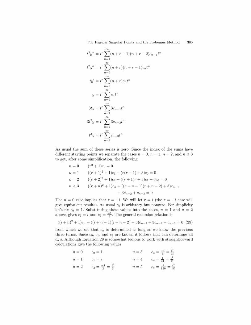
7.4 Regular Singular Points and the Frobenius Method 305
t3y′′ = tr∞∑
n=1
(n+ r − 1)(n+ r − 2)cn−1tn
t2y′′ = tr∞∑
n=0
(n+ r)(n+ r − 1)cntn
ty′ = tr∞∑
n=0
(n+ r)cntn
y = tr∞∑
n=0
cntn
3ty = tr∞∑
n=1
3cn−1tn
3t2y = tr∞∑
n=2
3cn−2tn
t3y = tr∞∑
n=3
cn−3tn
As usual the sum of these series is zero. Since the index of the sums havedifferent starting points we separate the cases n = 0, n = 1, n = 2, and n ≥ 3to get, after some simplification, the following
n = 0 (r2 + 1)c0 = 0
n = 1 ((r + 1)2 + 1)c1 + (r(r − 1) + 3)c0 = 0
n = 2 ((r + 2)2 + 1)c2 + ((r + 1)r + 3)c1 + 3c0 = 0
n ≥ 3 ((r + n)2 + 1)cn + ((r + n− 1)(r + n− 2) + 3)cn−1
+ 3cn−2 + cn−3 = 0
The n = 0 case implies that r = ±i. We will let r = i (the r = −i case willgive equivalent results). As usual c0 is arbitrary but nonzero. For simplicitylet’s fix c0 = 1. Substituting these values into the cases, n = 1 and n = 2above, gives c1 = i and c2 = −1
2 . The general recursion relation is
((i+ n)2 + 1)cn + ((i+ n− 1)(i+ n− 2) + 3)cn−1 + 3cn−2 + cn−3 = 0 (29)
from which we see that cn is determined as long as we know the previousthree terms. Since c0, c1, and c2 are known it follows that can determine allcn’s. Although Equation 29 is somewhat tedious to work with straightforwardcalculations give the following values
n = 0 c0 = 1 n = 3 c3 = −i6 = i3
3!
n = 1 c1 = i n = 4 c4 = 124 = i4
4!
n = 2 c2 = −12 = i2
2! n = 5 c5 = i120 = i5
5!
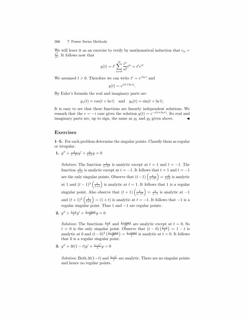
306 7 Power Series Methods
We will leave it as an exercise to verify by mathematical induction that cn =in
n! . It follows now that
y(t) = ti∞∑
n=0
in
n!tn = tieit
We assumed t > 0. Therefore we can write ti = ei ln t and
y(t) = ei(t+ln t).
By Euler’s formula the real and imaginary parts are
y1(t) = cos(t+ ln t) and y2(t) = sin(t+ ln t).
It is easy to see that these functions are linearly independent solutions. Weremark that the r = −i case gives the solution y(t) = e−i(t+ln t). Its real andimaginary parts are, up to sign, the same as y1 and y2 given above. J
Exercises
1–5. For each problem determine the singular points. Classify them as regularor irregular.
1. y′′ + t1−t2 y
′ + 11+ty = 0
Solution: The function t1−t2 is analytic except at t = 1 and t = −1. The
function 11+t is analytic except at t = −1. It follows that t = 1 and t = −1
are the only singular points. Observe that (t−1)(
t1−t2
)
= −t1+t is analytic
at 1 and (t − 1)2(
11+t
)
is analytic at t = 1. It follows that 1 is a regular
singular point. Also observe that (t + 1)(
t1−t2
)
= t1−t is analytic at −1
and (t+ 1)2(
11+t
)
= (1 + t) is analytic at t = −1. It follows that −1 is a
regular singular point. Thus 1 and −1 are regular points.
2. y′′ + 1−tt y′ + 1−cos t
t3 y = 0
Solution: The functions 1−tt and 1−cos t
t3 are analytic except at t = 0. Sot = 0 is the only singular point. Observe that (t − 0)
(
1−tt
)
= 1 − t isanalytic at 0 and (t− 0)2
(
1−cos tt3
)
= 1−cos tt is analytic at t = 0. It follows
that 0 is a regular singular point.
3. y′′ + 3t(1− t)y′ + 1−et
t y = 0
Solution: Both 3t(1−t) and 1−et
t are analytic. There are no singular pointsand hence no regular points.
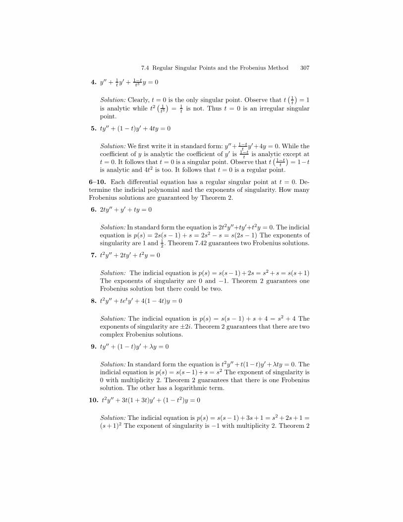
7.4 Regular Singular Points and the Frobenius Method 307
4. y′′ + 1t y
′ + 1−tt3 y = 0
Solution: Clearly, t = 0 is the only singular point. Observe that t(
1t
)
= 1
is analytic while t2(
1t3
)
= 1t is not. Thus t = 0 is an irregular singular
point.
5. ty′′ + (1− t)y′ + 4ty = 0
Solution: We first write it in standard form: y′′+ 1−tt y′+4y = 0. While the
coefficient of y is analytic the coefficient of y′ is 1−tt is analytic except at
t = 0. It follows that t = 0 is a singular point. Observe that t(
1−tt
)
= 1−tis analytic and 4t2 is too. It follows that t = 0 is a regular point.
6–10. Each differential equation has a regular singular point at t = 0. De-termine the indicial polynomial and the exponents of singularity. How manyFrobenius solutions are guaranteed by Theorem 2.
6. 2ty′′ + y′ + ty = 0
Solution: In standard form the equation is 2t2y′′+ty′+t2y = 0. The indicialequation is p(s) = 2s(s − 1) + s = 2s2 − s = s(2s− 1) The exponents ofsingularity are 1 and 1
2 . Theorem 7.42 guarantees two Frobenius solutions.
7. t2y′′ + 2ty′ + t2y = 0
Solution: The indicial equation is p(s) = s(s− 1)+2s = s2 + s = s(s+1)The exponents of singularity are 0 and −1. Theorem 2 guarantees oneFrobenius solution but there could be two.
8. t2y′′ + tety′ + 4(1− 4t)y = 0
Solution: The indicial equation is p(s) = s(s − 1) + s + 4 = s2 + 4 Theexponents of singularity are ±2i. Theorem 2 guarantees that there are twocomplex Frobenius solutions.
9. ty′′ + (1− t)y′ + λy = 0
Solution: In standard form the equation is t2y′′ + t(1− t)y′ +λty = 0. Theindicial equation is p(s) = s(s−1)+ s = s2 The exponent of singularity is0 with multiplicity 2. Theorem 2 guarantees that there is one Frobeniussolution. The other has a logarithmic term.
10. t2y′′ + 3t(1 + 3t)y′ + (1 − t2)y = 0
Solution: The indicial equation is p(s) = s(s− 1)+ 3s+ 1 = s2 + 2s+ 1 =(s+1)2 The exponent of singularity is −1 with multiplicity 2. Theorem 2
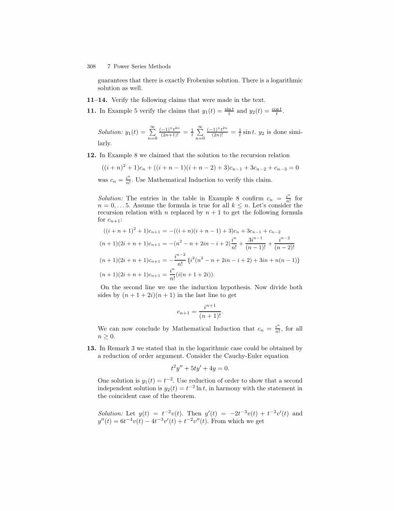
308 7 Power Series Methods
guarantees that there is exactly Frobenius solution. There is a logarithmicsolution as well.
11–14. Verify the following claims that were made in the text.
11. In Example 5 verify the claims that y1(t) = sin tt and y2(t) = cos t
t .
Solution: y1(t) =∞∑
n=0
(−1)nt2n
(2n+1)! = 1t
∞∑
n=0
(−1)nt2n
(2n)! = 1t sin t. y2 is done simi-
larly.
12. In Example 8 we claimed that the solution to the recursion relation
((i+ n)2 + 1)cn + ((i+ n− 1)(i+ n− 2) + 3)cn−1 + 3cn−2 + cn−3 = 0
was cn = in
n! . Use Mathematical Induction to verify this claim.
Solution: The entries in the table in Example 8 confirm cn = in
n! forn = 0, . . . 5. Assume the formula is true for all k ≤ n. Let’s consider therecursion relation with n replaced by n + 1 to get the following formulafor cn+1:
((i + n + 1)2 + 1)cn+1 = −((i + n)(i + n − 1) + 3)cn + 3cn−1 + cn−2
(n + 1)(2i + n + 1)cn+1 = −(n2 − n + 2in − i + 2)in
n!+
3in−1
(n − 1)!+
in−2
(n − 2)!
(n + 1)(2i + n + 1)cn+1 = − in−2
n! i2(n2 − n + 2in − i + 2) + 3in + n(n − 1)(n + 1)(2i + n + 1)cn+1 =
in
n!(i(n + 1 + 2i)).
On the second line we use the induction hypothesis. Now divide bothsides by (n+ 1 + 2i)(n+ 1) in the last line to get
cn+1 =in+1
(n+ 1)!.
We can now conclude by Mathematical Induction that cn = in
n! , for alln ≥ 0.
13. In Remark 3 we stated that in the logarithmic case could be obtained bya reduction of order argument. Consider the Cauchy-Euler equation
t2y′′ + 5ty′ + 4y = 0.
One solution is y1(t) = t−2. Use reduction of order to show that a secondindependent solution is y2(t) = t−2 ln t, in harmony with the statement inthe coincident case of the theorem.
Solution: Let y(t) = t−2v(t). Then y′(t) = −2t−3v(t) + t−2v′(t) andy′′(t) = 6t−4v(t)− 4t−3v′(t) + t−2v′′(t). From which we get
7.4 Regular Singular Points and the Frobenius Method 309
t2y′′ = 6t−2v(t)− 4t−1v′(t) + v′′(t)
5ty′ = −10t−2v(t) + 5t−1v′(t)
4y = 4t−2v(t).
Adding these terms and remembering that we are assuming the y is asolution we get
0 = t−1v′(t) + v′′(t).
From this we get v′′
v′= −1
t . Integrating we get ln v′(t) = − ln t and hencev′(t) = 1
t . Integrating again gives v(t) = ln t. It follows that y(t) = t−2 ln tis a second independent solution.
14. Verify the claim made in Example 6 that y1(t) = (t3 + 4t2)et
Solution:
y1(t) =
∞∑
n=0
n+ 4
n!tn+2
=∞∑
n=0
n
n!tn+2 +
∞∑
n=0
4
n!tn+2
= t3∞∑
n=1
tn−1
(n− 1)!+ 4t2
∞∑
n=0
tn
n!
= t3et + 4t2et = (t3 + 4t2)et.
15–26. Use the Frobenius method to solve each of the following differentialequations. For those problems marked with a (*) one of the independent so-lutions can easily be written in closed form. For those problems marked witha (**) both independent solutions can easily be written in closed form.
15. ty′′ − 2y′ + ty = 0 (**) (real roots; differ by integer; two Frobenius solu-tions)
Solution: Indicial polynomial: p(s) = s(s − 3); exponents of singularitys = 0 and s = 3.
n = 0 c0(r)(r − 3) = 0n = 1 c1(r − 2)(r + 1) = 0n ≥ 1 cn(n+ r)(n+ r − 3) = −cn−1
r=3:n odd cn = 0
n = 2m c2m = 3c0(−1)m(2m+2)
(2m+3)!
y(t) = 3c0∑∞
m=0(−1)m(2m+2)t2m+3
(2m+3)! = 3c0(sin t− t cos t).
310 7 Power Series Methods
r=0: One is lead to the equation 0c3 = 0 and we can take c3 = 0. Thus
n odd cn = 0
n = 2m c2m = c0(−1)m+1(2m−1)
(2m)!
y(t) = c0∑∞
m=0(−1)m+1(2m−1)t2m
(2m)! = c0(t sin t+ cos t).
General Solution: y = c1(sin t− t cos t) + c2(t sin t+ cos t).
16. 2t2y′′− ty′ +(1+ t)y = 0 (**) (real roots, do not differ by an integer, twoFrobenius solutions)
Solution: Indicial polynomial: p(s) = (2s− 1)(s− 1); exponents of singu-larity s = 1/2 and s = 1.
n = 0 c0(2r − 1)(r − 1) = 0n ≥ 1 cn(2(n+ r)− 1)(n+ r − 1) = −cn−1
r = 1: cn = −cn−1
(2n+1)n and hence
cn =(−1)n2nc0(2n+ 1)!
, n ≥ 1.
From this we get
y(t) = c0
∞∑
n=0
(−1)n2ntn+1
(2n+ 1)!
= c0
√t√2
∞∑
n=0
(−1)n(√
2t)2n+1
(2n+ 1)!
=c0√2
√t sin√
2t.
r = 1/2: The recursion relation becomes cn(2n − 1)(n) = −cn−1. Thecoefficient of cn is never zero for n ≥ 1 hence cn = −cn−1
n(2n−1) and hence
cn =(−1)n2n
(2n)!.
We now get
y(t) =
∞∑
n=0
(−1)n2ntn+1/2
(2n)!
=√t
∞∑
n=0
(−1)n(√
2t)2n
(2n)!
=√t cos
√2t.
7.4 Regular Singular Points and the Frobenius Method 311
General Solution: y = c1√t sin√
2t+ c2√t cos
√2t.
17. t2y′′ − t(1 + t)y′ + y = 0, (*) (real roots, coincident, logarithmic case)
Solution: Indicial polynomial: p(s) = (s − 1)2; exponents of singularitys = 1, multiplicity 2. There is one Frobenius solution.
r = 1 : Let y(t) =∑∞
n=0 cntn+1. Then
n ≥ 1 n2cn − ncn−1 = 0.
This is easy to solve. We get cn = 1n!c0 and hence
y(t) = c0
∞∑
n=0
1
n!tn+1 = c0te
t.
Logarithmic Solution: Let y1(t) = tet. The second independent solutionis necessarily of the form
y(t) = y1(t) ln t+
∞∑
n=0
cntn+1.
Substitution into the differential equation leads to
t2et +
∞∑
n=1
(n2cn − ncn−1)tn+1 = 0.
We write out the power series for t2et and add corresponding coefficientsto get
n2cn − ncn−1 +1
(n− 1)!.
The following list is a straightforward verification:
n = 1 c1 = −1
n = 2 c2 = −12
(
1 + 12
)
n = 3 c3 = −13!
(
1 + 12 + 1
3
)
n = 4 c4 = −14!
(
1 + 12 + 1
3 + 14
)
.
Let sn = 1 + 12 + · · ·+ 1
n . Then an easy argument gives that
cn =−sn
n!.
We now have a second independent solution
312 7 Power Series Methods
y2(t) = tet ln t− t∞∑
n=1
sntn
n!.
General Solution:
y = c1tet + c2
(
tet ln t− t∞∑
n=1
sntn
n!
)
.
18. 2t2y′′− ty′ +(1− t)y = 0 (**) (real roots, do not differ by an integer, twoFrobenius solutions)
Solution: Indicial polynomial: p(s) = (2s− 1)(s− 1); exponents of singu-larity s = 1/2 and s = 1.
n = 0 c0(2r − 1)(r − 1) = 0n ≥ 1 cn(2(n+ r) − 1)(n+ r − 1) = cn−1
r = 1: cn = cn−1
(2n+1)n and hence
cn =2nc0
(2n+ 1)!, n ≥ 1.
From this we get
y(t) = c0
∞∑
n=0
2ntn+1
(2n+ 1)!
= c0
√t√2
∞∑
n=0
(√
2t)2n+1
(2n+ 1)!
=c0√2
√t sinh
√2t.
r = 1/2: The recursion relation becomes cn(2n − 1)(n) = cn−1. Thecoefficient of cn is never zero for n ≥ 1 hence cn = cn−1
n(2n−1) and hence
cn =2n
(2n)!.
We now get
y(t) =
∞∑
n=0
2ntn+1/2
(2n)!
=√t
∞∑
n=0
(√
2t)2n
(2n)!
=√t cosh
√2t.
7.4 Regular Singular Points and the Frobenius Method 313
General Solution: y = c1√t sinh
√2t+ c2
√t cosh
√2t.
19. t2y′′ + t2y′ − 2y = 0 (**) (real roots; differ by integer; two Frobeniussolutions)
Solution: Indicial polynomial: p(s) = (s−2)(s+1); exponents of singularitys = 2 and s = −1.
n = 0 c0(r − 2)(r + 1) = 0n ≥ 1 cn(n+ r − 2)(n+ r + 1) = −cn−1(n+ r − 1)
s=2:
cn = 6c0(−1)n(n+ 1)
(n+ 3)!, n ≥ 1
y(t) = 6c0∑∞
n=0(−1)n(n+1)tn
(n+3)! = 6c0
(
(t+2)e−t
t + t−2t
)
.
s=-1: The recursion relation becomes cn(n − 3)(n) = cn−1(n − 2) = 0.Thus
n = 1 c1 = − c0
2n = 2 c2 = 0n = 3 0c3 = 0
We can take c3 = 0 and then cn = 0 for all n ≥ 2. We now have y(t) =c0t
−1(1 − t2 ) = c0
2
(
2−tt
)
.
General Solution: y = c12−t
t + c2(t+2)e−t
t .
20. t2y′′ + 2ty′ − a2t2y = 0 (**) (real roots, differ by integer, two FrobeniusSolutions)
Solution: Indicial polynomial: p(s) = s(s + 1); exponents of singularityr = 0 and r = −1.
n = 0 c0r(r + 1) = 0n = 1 c1(r + 1)(r + 2) = 0n ≥ 1 cn(n+ r)(n + r + 1) = a2cn−2
r = 0: In the case c1 = 0 and c2n+1 = 0 for all n ≥ 0. We also getc2n = a2c0
2n(2n+1) , n ≥ 1 which gives c2n = c0a2n
(2n+1)! . Thus
y(t) = c0
∞∑
n=0
(at)2n
(2n+ 1)!
=c0at
∞∑
n=0
(at)2n+1
(2n+ 1)!
=c0at
sinh at.
314 7 Power Series Methods
r = −1: The n = 1 case gives 0c1 = 0 so c1 may be arbitrary. Thereis no inconsistency. We choose c1 = 0. The recursion relation becomescn(n − 1)(n) = a2cn−2 and it is straightforward to see that c2n+1 = 0
while c2n = a2nc0
(2n)! . Thus
y(t) = c0
∞∑
n=0
a2nt2n−1
(2n)!
=c0t
∞∑
n=0
(at)2n
(2n)!
=c0t
coshat.
General Solution: y = c1cosh at
t + c2sinh at
t .
21. ty′′+(t−1)y′−2y = 0, (*) (real roots, differ by integer, logarithmic case)
Solution: Indicial polynomial: p(s) = s(s − 2); exponents of singularityr = 0 and r = 2.
n = 0 c0r(r − 2) = 0n ≥ 1 cn(n+ r)(n + r − 2) = −cn−1(n+ r − 3)
r=2: The recursion relation becomes cn = − n−1n(n+2)cn−1. For n = 1 we
see that c1 = 0 and hence cn = 0 for all n ≥ 1. It follows that y(t) = c0t2
is a solution.
r=0: The recursion relation becomes cn(n)(n − 2) = −cn−1(n − 3) = 0.Thus
n = 1 −c1 = − c0
−2
n = 2 0c2 = −2c0 ⇒⇐The n = 2 case implies an inconsistency in the recursion relation sincec0 6= 0. Since y1(t) = t2 is a Frobenius solution a second independentsolution can be written in the form
y(t) = t2 ln t+
∞∑
n=0
cntn.
Substitution leads to
t3 + 2t2 + (−c1 − 2c0)t+
∞∑
n=2
(cn(n)(n− 2) + cn−1(n− 3))tn = 0
and the following relations:
7.4 Regular Singular Points and the Frobenius Method 315
n = 1 −c1 − 2c0 = 0n = 2 2− c1 = 0n = 3 1 + 3c3 = 0n ≥ 4 n(n− 2)cn + (n− 3)cn−3 = 0.
We now have c0 = −1, c1 = 2, c3 = −1/3. c2 can be arbitrary so we choosec2 = 0, and cn = −(n−3)cn−1
n(n−2) , for n ≥ 4. A straightforward calculationgives
cn =2(−1)n
n!(n− 2).
A second independent solution is
y2(t) = t2 ln t+
(
−1 + 2t− t3
3+
∞∑
n=4
2(−1)ntn
n!(n− 2)
)
.
General Solution: y = c1t2 + c2y2(t).
22. ty′′ − 4y = 0 (real roots, differ by an integer, logarithmic case)
Solution: Write the differential equation in standard form: t2y′′−4ty = 0.Clearly, the indicial polynomial is p(s) = s(s−1); exponents of singularityare r = 0 and r = 1.
r=1: Let
y(t) =
∞∑
n=0
cntn+1, c0 6= 0.
Thenn ≥ 1 cn(n+ 1)(n) = 4cn−1
It follows that cn = 4nc0
(n+1)!n! , for all n ≥ 1 (notice that when n = 0 we get
c0). Hence y(t) = c0∑∞
n=04ntn+1
(n+1)!n! = c0
4
∑∞n=0
(4t)n+1
(n+1)!n! .
r = 0: When r = 0 the recursion relations become
cn(n)(n− 1) = 4cn−1, n ≥ 1
and hence when n = 1 we get 0c1 = 4c0, an inconsistency as c0 6= 0.There is no second Frobenius solution. However, there is a second linearlyindependent solution of the form y(t) = y1(t) ln t +
∑∞n=0 cnt
n, where
y1(t) =∑∞
n=0(4t)n+1
(n+1)!n! . Substituting this equation into the differentialequation and simplifying leads to the recursion relation
n(n− 1)cn = 4cn−1 −(2n− 1)4n
(n+ 1)!n!, n ≥ 1.
316 7 Power Series Methods
When n = 1 we get 0 = 0c1 = 4c0 − 2 and this implies c0 = 12 . Then the
recursion relation for n = 1 becomes 0c1 = 0, no inconsistency; we willchoose c1 = 0. The above recursion relation is difficult to solve. We givethe first few terms:
c0 = 12 c1 = 0
c2 = −2 c3 = −4627
c4 = −251405
It now follows that
y2(t) = y1(t) ln t+
(
1
2− 2t2 − 46
27t3 − 251
405t4 + · · ·
)
.
23. t2(−t+ 1)y′′ + (t+ t2)y′ + (−2t+ 1)y = 0 (**) (complex)
Solution: Indicial polynomial: p(s) = (s2 + 1); exponents of singularityr = ±i. Let r = i (the case r = −i gives equivalent results). The recursionrelation that arises from y(t) =
∑∞n=0 cnt
n+i is cn((n+i)2+1)−cn−1((n−2 + i)2 + 1) = 0 and hence
cn =(n− 2)(n− 2 + 2i)
n(n+ 2i)cn−1.
A straightforward calculation gives the first few terms as follows:
n = 1 c1 = 1−2i1+2ic0
n = 2 c2 = 0
n = 3 c3 = 0
and hence cn = 0 for all n ≥ 2. Therefore y(t) = c0(ti +
(
1−2i1+2i)
)
t1+i.
Since t > 0 we can write ti = ei ln t = cos ln t+i sin ln t, by Euler’s formula.Separating the real and imaginary parts we get two independent solutions
y1(t) = −3 cos ln t− 4 sin ln t+ 5t cos ln t
y2(t) = −3 sin ln t+ 4 cos ln t+ 5t sin ln t.
24. t2y′′ + t(1 + t)y′ − 2y = 0, (**) (real roots, differ by an integer, twoFrobenius solutions)
Solution: Indicial polynomial: p(s) = (s−1)(s+1); exponents of singularityr = 1 and r = −1.
n = 0 c0(r − 1)(r + 1) = 0n ≥ 1 cn(n+ r − 1)(n+ r + 1) = −cn−1(n+ r − 1)
7.4 Regular Singular Points and the Frobenius Method 317
r = 1 : The recursion relation becomes cn(n(n+2)) = −ncn−1 and hence
cn =2(−1)nc0(n+ 2)!
.
We then get
y(t) =
∞∑
n=0
cntn+1
= 2c0
∞∑
n=0
(−1)ntn+1
(n+ 2)!
=2c0t
∞∑
n=0
(−t)n+2
(n+ 2)!
=2c0t
(e−t − (1− t))
= 2c0
(
e−t − (1 − t)t
)
.
r = −1: The recursion relation becomes cn(n − 2)(n) = −cn−1(n − 2).Thus
n = 1 c1 = −c0n = 2 0c2 = 0
Thus c2 can be arbitrary so we can take c2 = 0 and then cn = 0 for alln ≥ 2. We now have
y(t) =
∞∑
n=0
cntn−1 = c0(t
−1 − 1) = c01− tt
.
General Solution: y = c11−t
t + c2e−t
t .
25. t2y′′ + t(1 − 2t)y′ + (t2 − t+ 1)y = 0 (**) (complex)
Solution: Indicial polynomial: p(s) = (s2 + 1); exponents of singularityr = ±i. Let r = i (the case r = −i gives equivalent results). The recursionrelation that arises from y(t) =
∑∞n=0 cnt
n+i is
n = 1 c1 = c0n ≥ 2 cn((n+ i)2 + 1) + cn−1(−2n− 2i+ 1) + cn−2 = 0
A straightforward calculation gives the first few terms as follows:
n = 1 c1 = c0n = 2 c2 = 1
2!c0n = 3 c3 = 1
3!c0n = 4 c4 = 1
4!c0.
318 7 Power Series Methods
An easy induction argument gives
cn =1
n!c0.
We now get
y(t) =∞∑
n=0
cntn+i
= c0
∞∑
n=0
tn+i
n!
= c0tiet.
Since t > 0 we can write ti = ei ln t = cos ln t+i sin ln t, by Euler’s formula.Now separating the real and imaginary parts we get two independentsolutions
y1(t) = et cos ln t and y2(t) = et sin ln t.
26. t2(1+ t)y′′− t(1+2t)y′+(1+2t)y = 0 (**) (real roots, equal, logarithmiccase)
Solution: Indicial polynomial: p(s) = (s − 1)2; exponents of singularitys = 1 with multiplicity 2.
r=1: Let
y(t) =∞∑
n=0
cntn+1, c0 6= 0.
Thenn = 1 c1 = 0n ≥ 2 n2cn = −cn−1(n− 2)
It follows that cn = 0 for all n ≥ 1. Hence y(t) = c0t. Let y1(t) = t.
logarithmic case: Let y(t) = t ln t+∑∞
n=0 cntn+1.The recursion relations
becomesn = 0 −c0 + c0 = 0n = 1 c1 = 1n ≥ 2 n2cn = −(n− 1)(n− 2)cn−1
The n = 0 case allows us to choose c0 arbitrarily. We choose c0 = 0. Forn ≥ 2 it is easily to see the cn = 0. Hence y(t) = t ln t+ t2.
general solution: y(t) = a1t+ a2(t ln t+ t2).
7.5 Laplace Inversion involving Irreducible Quadratics 319
7.5 Application of the Frobenius Method:
Laplace Inversion involving Irreducible Quadratics
In Section 3.8 we considered the problem of finding the inverse Laplace trans-form of simple rational functions with powers of an irreducible quadratic inthe denominator. After some reductions involving the First Translation Prin-ciple and the Dilation Principle we reduced the problem to simple rationalfunctions of the form
1
(s2 + 1)k+1and
s
(s2 + 1)k+1,
where k is a nonnegative integer. Thereafter we derived a recursion formulathat determines the inversion for all such rational functions. In this section wewill derive a closed formula for the inversion by solving a distinguished secondorder differential equation, with a regular singular point at t = 0, associatedto each simple rational function given above.
Recall from Section 3.5 that Ak(t) and Bk(t) were defined by the relations
1
2kk!LAk(t) =
1
(s2 + 1)k+1
1
2kk!LBk(t) =
s
(s2 + 1)k+1.
(1)
Also, recall from Theorem 3.5.7 that
Bk+1(t) = tAk(t). (2)
Lemma 1. Suppose k ≥ 1. Then
Ak(0) = 0 and Bk(0) = 0.
Proof. By the Initial Value Theorem, Theorem 6.4.3,
Ak(0) = 2kk! lims→∞
s
(s2 + 1)k+1= 0
Bk(0) = 2kk! lims→∞
s2
(s2 + 1)k+1= 0
ut
Proposition 2. Suppose k ≥ 1. Then
A′k(t) = Bk(t) (3)
B′k(t) = 2kAk−1(t)−Ak(t). (4)
320 7 Power Series Methods
Proof. By the Input Derivative Principle and the Lemma above we have
1
2kk!LA′
k(t) =1
2kk!(sLAk(t) −Ak(0))
=s
(s2 + 1)k+1
=1
2kk!LBk(t) .
Equation (3) now follows. In a similar way we have
1
2kk!LB′
k(t) =1
2kk!(sLBk(t) −Bk(0))
=s2
(s2 + 1)k+1
=1
(s2 + 1)k− 1
(s2 + 1)k+1
=2k
2kk!LAk−1(t) −
1
2kk!LAk(t) .
Equation (4) now follows. ut
Proposition 3. With notation as above we have
tA′′k − 2kA′
k + tAk = 0 (5)
t2B′′k − 2ktB′
k + (t2 + 2k)Bk = 0. (6)
Proof. We first differentiate Equation (3) and then substitute in Equation (4)to get
A′′k = B′
k = 2kAk−1 −Ak.
Now multiply this equation by t and simplify using Equations (2) and (3) toget
tA′′k = 2ktAk−1 − tAk = 2kBk − tAk = 2kA′
k − tAk.
Equation (5) now follows. To derive Equation (6) first differentiate Equation(5) and then multiply by t to get
t2A′′′k + (1 − 2k)tA′′
k + t2A′k + tAk = 0.
From Equation (5) we get tAk = −tA′′k + 2kA′
k which we substitute into theequation above to get
t2A′′′k − 2ktA′′
k + (t2 + 2k)A′k = 0.
Equation (6) follows now from Equation (3). ut
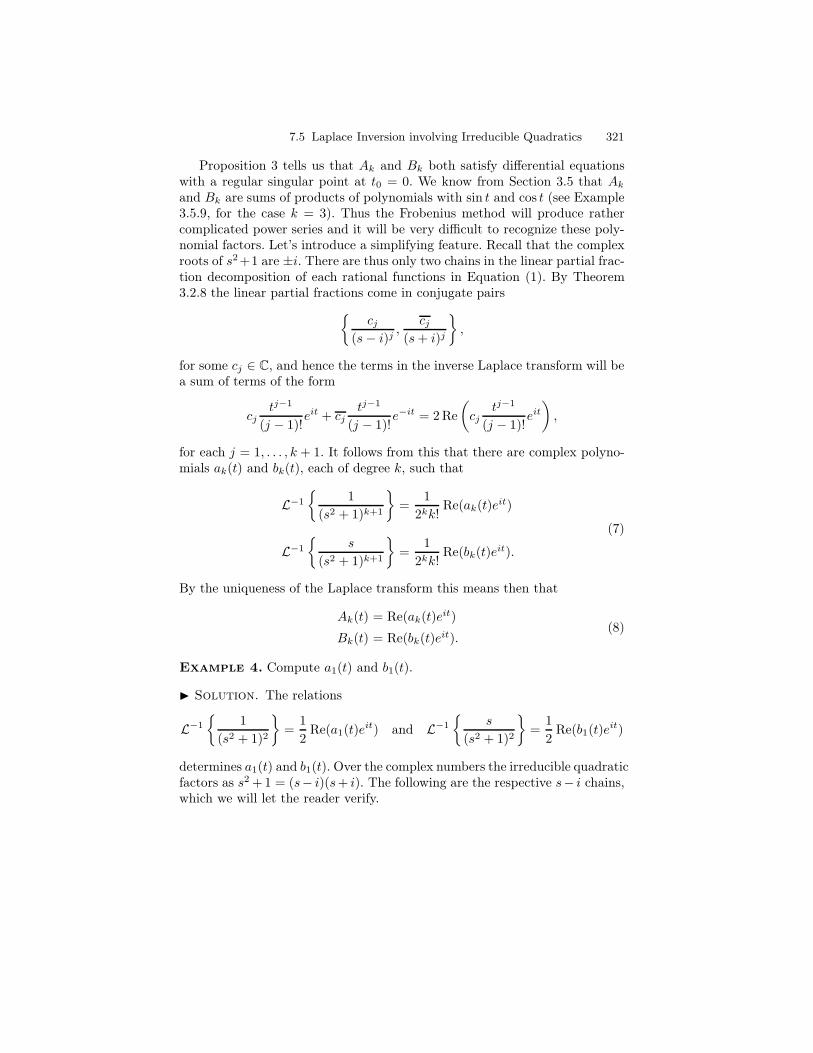
7.5 Laplace Inversion involving Irreducible Quadratics 321
Proposition 3 tells us that Ak and Bk both satisfy differential equationswith a regular singular point at t0 = 0. We know from Section 3.5 that Ak
and Bk are sums of products of polynomials with sin t and cos t (see Example3.5.9, for the case k = 3). Thus the Frobenius method will produce rathercomplicated power series and it will be very difficult to recognize these poly-nomial factors. Let’s introduce a simplifying feature. Recall that the complexroots of s2+1 are ±i. There are thus only two chains in the linear partial frac-tion decomposition of each rational functions in Equation (1). By Theorem3.2.8 the linear partial fractions come in conjugate pairs
cj(s− i)j
,cj
(s+ i)j
,
for some cj ∈ C, and hence the terms in the inverse Laplace transform will bea sum of terms of the form
cjtj−1
(j − 1)!eit + cj
tj−1
(j − 1)!e−it = 2 Re
(
cjtj−1
(j − 1)!eit
)
,
for each j = 1, . . . , k + 1. It follows from this that there are complex polyno-mials ak(t) and bk(t), each of degree k, such that
L−1
1
(s2 + 1)k+1
=1
2kk!Re(ak(t)eit)
L−1
s
(s2 + 1)k+1
=1
2kk!Re(bk(t)eit).
(7)
By the uniqueness of the Laplace transform this means then that
Ak(t) = Re(ak(t)eit)
Bk(t) = Re(bk(t)eit).(8)
Example 4. Compute a1(t) and b1(t).
I Solution. The relations
L−1
1
(s2 + 1)2
=1
2Re(a1(t)e
it) and L−1
s
(s2 + 1)2
=1
2Re(b1(t)e
it)
determines a1(t) and b1(t). Over the complex numbers the irreducible quadraticfactors as s2 +1 = (s− i)(s+ i). The following are the respective s− i chains,which we will let the reader verify.
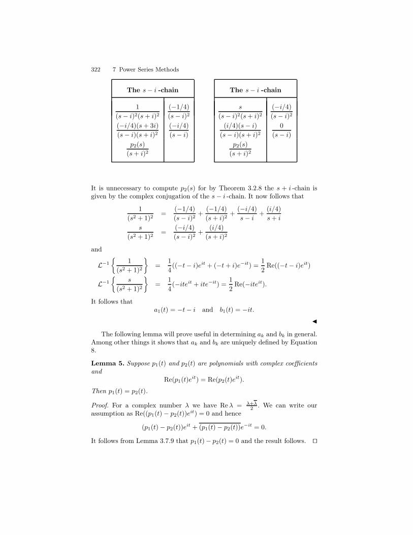
322 7 Power Series Methods
The s− i -chain
1
(s− i)2(s+ i)2(−1/4)
(s− i)2(−i/4)(s+ 3i)
(s− i)(s+ i)2(−i/4)
(s− i)p2(s)
(s+ i)2
The s− i -chain
s
(s− i)2(s+ i)2(−i/4)
(s− i)2(i/4)(s− i)
(s− i)(s+ i)20
(s− i)p2(s)
(s+ i)2
It is unnecessary to compute p2(s) for by Theorem 3.2.8 the s + i -chain isgiven by the complex conjugation of the s− i -chain. It now follows that
1
(s2 + 1)2=
(−1/4)
(s− i)2 +(−1/4)
(s+ i)2+
(−i/4)
s− i +(i/4)
s+ i
s
(s2 + 1)2=
(−i/4)
(s− i)2 +(i/4)
(s+ i)2
and
L−1
1
(s2 + 1)2
=1
4((−t− i)eit + (−t+ i)e−it) =
1
2Re((−t− i)eit)
L−1
s
(s2 + 1)2
=1
4(−iteit + ite−it) =
1
2Re(−iteit).
It follows thata1(t) = −t− i and b1(t) = −it.
J
The following lemma will prove useful in determining ak and bk in general.Among other things it shows that ak and bk are uniquely defined by Equation8.
Lemma 5. Suppose p1(t) and p2(t) are polynomials with complex coefficientsand
Re(p1(t)eit) = Re(p2(t)e
it).
Then p1(t) = p2(t).
Proof. For a complex number λ we have Reλ = λ+λ2 . We can write our
assumption as Re((p1(t)− p2(t))eit) = 0 and hence
(p1(t)− p2(t))eit + (p1(t)− p2(t))e
−it = 0.
It follows from Lemma 3.7.9 that p1(t)− p2(t) = 0 and the result follows. ut
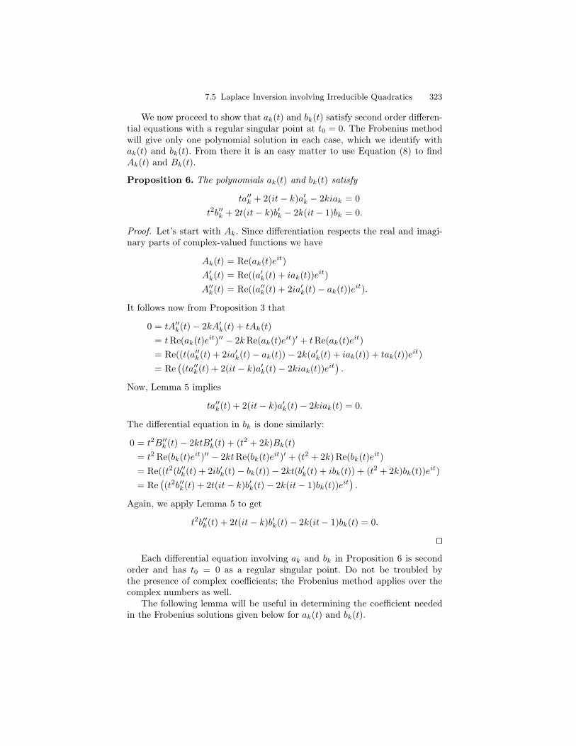
7.5 Laplace Inversion involving Irreducible Quadratics 323
We now proceed to show that ak(t) and bk(t) satisfy second order differen-tial equations with a regular singular point at t0 = 0. The Frobenius methodwill give only one polynomial solution in each case, which we identify withak(t) and bk(t). From there it is an easy matter to use Equation (8) to findAk(t) and Bk(t).
Proposition 6. The polynomials ak(t) and bk(t) satisfy
ta′′k + 2(it− k)a′k − 2kiak = 0
t2b′′k + 2t(it− k)b′k − 2k(it− 1)bk = 0.
Proof. Let’s start with Ak. Since differentiation respects the real and imagi-nary parts of complex-valued functions we have
Ak(t) = Re(ak(t)eit)
A′k(t) = Re((a′k(t) + iak(t))eit)
A′′k(t) = Re((a′′k(t) + 2ia′k(t)− ak(t))eit).
It follows now from Proposition 3 that
0 = tA′′k(t)− 2kA′
k(t) + tAk(t)
= tRe(ak(t)eit)′′ − 2kRe(ak(t)eit)′ + tRe(ak(t)eit)
= Re((t(a′′k(t) + 2ia′k(t)− ak(t)) − 2k(a′k(t) + iak(t)) + tak(t))eit)
= Re(
(ta′′k(t) + 2(it− k)a′k(t)− 2kiak(t))eit)
.
Now, Lemma 5 implies
ta′′k(t) + 2(it− k)a′k(t)− 2kiak(t) = 0.
The differential equation in bk is done similarly:
0 = t2B′′k (t)− 2ktB′
k(t) + (t2 + 2k)Bk(t)
= t2 Re(bk(t)eit)′′ − 2ktRe(bk(t)eit)′ + (t2 + 2k)Re(bk(t)eit)
= Re((t2(b′′k(t) + 2ib′k(t)− bk(t))− 2kt(b′k(t) + ibk(t)) + (t2 + 2k)bk(t))eit)
= Re(
(t2b′′k(t) + 2t(it− k)b′k(t)− 2k(it− 1)bk(t))eit)
.
Again, we apply Lemma 5 to get
t2b′′k(t) + 2t(it− k)b′k(t)− 2k(it− 1)bk(t) = 0.
utEach differential equation involving ak and bk in Proposition 6 is second
order and has t0 = 0 as a regular singular point. Do not be troubled bythe presence of complex coefficients; the Frobenius method applies over thecomplex numbers as well.
The following lemma will be useful in determining the coefficient neededin the Frobenius solutions given below for ak(t) and bk(t).
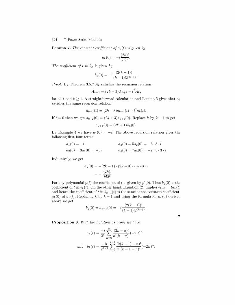
324 7 Power Series Methods
Lemma 7. The constant coefficient of ak(t) is given by
ak(0) = −i (2k)!k!2k
.
The coefficient of t in bk is given by
b′k(0) = −i (2(k − 1))!
(k − 1)!2(k−1).
Proof. By Theorem 3.5.7 Ak satisfies the recursion relation
Ak+2 = (2k + 3)Ak+1 − t2Ak,
for all t and k ≥ 1. A straightforward calculation and Lemma 5 gives that ak
satisfies the same recursion relation:
ak+2(t) = (2k + 3)ak+1(t)− t2ak(t).
If t = 0 then we get ak+2(0) = (2k + 3)ak+1(0). Replace k by k − 1 to get
ak+1(0) = (2k + 1)ak(0).
By Example 4 we have a1(0) = −i. The above recursion relation gives thefollowing first four terms:
a1(0) = −i a3(0) = 5a2(0) = −5 · 3 · ia2(0) = 3a1(0) = −3i a4(0) = 7a3(0) = −7 · 5 · 3 · i
Inductively, we get
ak(0) = −(2k − 1) · (2k − 3) · · · 5 · 3 · i
= −i (2k)!k!2k
.
For any polynomial p(t) the coefficient of t is given by p′(0). Thus b′k(0) is thecoefficient of t in bk(t). On the other hand, Equation (2) implies bk+1 = tak(t)and hence the coefficient of t in bk+1(t) is the same as the constant coefficient,ak(0) of ak(t). Replacing k by k − 1 and using the formula for ak(0) derivedabove we get
b′k(0) = ak−1(0) = −i (2(k − 1))!
(k − 1)!2(k−1).
J
Proposition 8. With the notation as above we have
ak(t) =−i2k
k∑
n=0
(2k − n)!
n!(k − n)!(−2it)n
and bk(t) =−it2k−1
k−1∑
n=0
(2(k − 1)− n)!
n!(k − 1− n)!(−2it)n.
7.5 Laplace Inversion involving Irreducible Quadratics 325
Proof. By Proposition 6, ak(t) is the polynomial solution to the differentialequation
ty′′ + 2(it− k)y′ − 2kiy = 0 (9)
with constant coefficient ak(0) as given in Lemma 7. Multiplying Equation(9) by t gives t2y′′ + 2t(it − k)y′ − 2kity = 0 which is easily seen to have aregular singular point at t = 0. The indicial polynomial is given by q(s) =s(s − 1)− 2ks = s(s− (2k + 1)). It follows that the exponents of singularityare 0 and 2k + 1. We will show below that the r = 0 case gives a polynomialsolution. We leave it to the exercises to verify that the r = 2k + 1 case givesa non polynomial Frobenius solution. We thus let
y(t) =
∞∑
n=0
cntn.
Then
ty′′(t) =
∞∑
n=1
(n)(n+ 1)cn+1tn
2ity′(t) =
∞∑
n=1
2incntn
−2ky′(t) =∞∑
n=0
−2k(n+ 1)cn+1tn
−2iky(t) =
∞∑
n=0
−2ikcntn
By assumption the sum of the series is zero. We separate the n = 0 and n ≥ 1cases and simplify to get
n = 0 −2kc1 − 2ikc0 = 0n ≥ 1 (n− 2k)(n+ 1)cn+1 + 2i(n− k)cn = 0
(10)
The n = 0 case tells us that c1 = −c0. For 1 ≤ n ≤ 2k − 1 we have
cn+1 =−2i(k − n)
(2k − n)(n+ 1)cn.
Observe that ck+1 = 0 and hence cn = 0 for all k+1 ≤ n ≤ 2k−1. For n = 2kwe get from the recursion relation 0c2k+1 = 2ikck = 0. This implies that c2k+1
can be arbitrary. We will choose c2k+1 = 0. Then cn = 0 for all n ≥ k + 1and hence the solution y is a polynomial. We make the usual comment that ifck+1 is chosen to be nonzero then the those terms with ck+1 as a factor willmake up the Frobenius solution for exponent of singularity r = 2k + 1. Let’snow determine the coefficients cn for 0 ≤ n ≤ k. From the recursion relation,Equation (10), we get
326 7 Power Series Methods
n = 0 c1 = −ic0n = 1 c2 = −2i(k−1)
(2k−1)2 c1 = 2(−i)2(k−1)(2k−1)2 = (−2i)2k(k−1)
(2k)(2k−1)2
n = 2 c3 = −2i(k−2)(2k−2)3 c2 = (−2i)3k(k−1)(k−2)
2k(2k−1)(2k−2)3! c0
n = 3 c4 = −2i(k−3)(2k−3)4 c3 = (−2i)4k(k−1)(k−2)(k−3)
2k(2k−1)(2k−2)(2k−3)4! c0
and generally,
cn =(−2i)nk(k − 1) · · · (k − n+ 1)
2k(2k − 1) · · · (2k − n+ 1)n!n = 1, . . . , k.
We can write this more compactly in terms of binomial coefficients as
cn =(−2i)n
(
kn
)
(
2kn
)
n!.
It follows now that
y(t) = c0
k∑
n=0
(−2i)n(
kn
)
(
2kn
)
n!tn.
The constant coefficient is c0. Thus we choose c0 = ak(0) as given in Lemma7. Then y(t) = ak(t) is the polynomial solution we seek. We get
ak(t) = ak(0)
k∑
n=0
(−2i)n(
kn
)
(
2kn
)
n!tn
=
k∑
n=0
−i (2k)!k!2k
(−2i)n(
kn
)
(
2kn
)
n!tn
=−i2k
k∑
n=0
(2k − n)!
(k − n)!n!(−2it)n.
It is easy to check that Equation (2) has as an analogue the equation bk+1(t) =tak(t). Replacing k by k−1 in the formula for ak(t) and multiplying by t thusestablishes the formula for bk(t). J
For x ∈ R we let [x] denote the greatest integer function. It is defined tobe the greatest integer less than or equal to x. For example, [1.5] = 1 and[2] = 2. We are now in a position to give a closed formula for the inverseLaplace transforms of the simple rational functions given in Equation (7).
Theorem 9. For the simple rational functions we have:
7.5 Laplace Inversion involving Irreducible Quadratics 327
Simple Irreducible Quadratics
L−1
1(s2+1)k+1
(t) = sin t22k
[ k2 ]∑
m=0
(−1)m(
2k−2m
k
) (2t)2m
(2m)!
− cos t22k
[ k−12 ]∑
m=0
(−1)m(
2k−2m−1k
) (2t)2m+1
(2m+1)!
L−1
s(s2+1)k+1
(t) = t sin tk·22k−1
[ k−12 ]∑
m=0
(−1)m(
2k−2m−2k−1
) (2t)2m
(2m)!
− t cos tk·22k−1
[ k−22 ]∑
m=0
(−1)m(
2k−2m−3k−1
) (2t)2m+1
(2m+1)!.
Proof. From Proposition 8 we can write
ak(t) =1
2k
k∑
n=0
(2k − n)!
n!(k − n)!(−1)n+1(i)n+1(2t)n.
It is easy to see that the real part of ak consists of those terms where n is odd.The imaginary part (up to the factor of i) consists of those terms where n iseven. The odd integers from n = 0, . . . , k can be written n = 2m + 1 wherem = 0, . . . ,
[
k−12
]
. Similarly, the even integers can be written n = 2m, wherem = 0, . . . ,
[
k2
]
. We thus have
Re(ak(t)) =1
2k
[ k−12 ]∑
m=0
(2k − 2m− 1)!
(2m+ 1)!(k − 2m− 1)!(−1)2m+2(i)2m+2(2t)2m+1
=−1
2k
[ k−12 ]∑
m=0
(2k − 2m− 1)!
(2m+ 1)!(k − 2m− 1)!(−1)m(2t)2m+1
and
328 7 Power Series Methods
Im(ak(t)) =1
i
1
2k
[ k2 ]∑
m=0
(2k − 2m)!
(2m)!(k − 2m)!(−1)2m+1(i)2m+1(2t)2m
=−1
2k
[ k2 ]∑
m=0
(2k − 2m)!
(2m)!(k − 2m)!(−1)m(2t)2m.
Now Re(ak(t)eit) = Re(ak(t)) cos t− Im(ak(t)) sin t. It follows from Equation7 that
L−1
1
(s2 + 1)k+1
=1
2kk!Re(ak(t)eit)
=1
2kk!Re(ak(t)) cos t− 1
2kk!Im(ak(t)) sin t
=− cos t
22k
[ k−12 ]∑
m=0
(2k − 2m− 1)!
k!(2m+ 1)!(k − 2m− 1)!(−1)m(2t)2m+1
+sin t
22k
[ k2 ]∑
m=0
(2k − 2m)!
k!(2m)!(k − 2m)!(−1)m(2t)2m
=− cos t
22k
[ k−12 ]∑
m=0
(
2k − 2m− 1
k
)
(−1)m (2t)2m+1
(2m+ 1)!
+sin t
22k
[ k2 ]∑
m=0
(
2k − 2m
k
)
(−1)m (2t)2m
(2m)!.
A similar calculation gives the formula for L−1
s(s2+1)k+1
. ut
Exercises
1–3.
1. Verify the statement made that the Frobenius solution to
ty′′ + 2(it − k)y′ − 2kiy = 0
with exponent of singularity r = 2k + 1 is not a polynomial.
2. Use the Frobenius method on the differential equation
t2y′′ + 2t(it − k)y′ − 2k(it − 1) = 0.
Verify that the indicial polynomial is q(s) = (s − 1)(s − 2k). Show that forthe exponent of singularity r = 1 there is a polynomial solution while for theexponent of singularity r = 2k there is not a polynomial solution. Verify theformula for bk(t) given in Proposition 8.
7.5 Laplace Inversion involving Irreducible Quadratics 329
3. Verify the formula for the inverse Laplace transform ofs
(s2 + 1)k+1given in
Theorem 9.
4–11. This series of exercises leads to closed formulas for the inverseLaplace transform of
1
(s2 − 1)k+1and
s
(s2 − 1)k+1.
Define Ck(t) and Dk(t) by the formulas
1
2kk!LCk(t) (s) =
1
(s2 − 1)k+1
and1
2kk!LDk(t) (s) =
s
(s2 − 1)k+1.
4. Show the following:
1. Ck+2(t) = t2Ck(t) − (2k + 3)Ck+1(t)
2. Dk+2(t) = t2Dk(t) − (2k + 1)Dk+1(t)
3. tCk(t) = Dk+1(t).
5. Show the following: For k ≥ 1
1. C′k(t) = Dk(t)
2. D′k(t) = 2kCk−1(t) + Ck(t).
6. Show the following:
1. tC′′k (t) − 2kC′
k(t) − tCk(t) = 0
2. t2D′′k (t) − 2ktD′
k(t) = (2k − t2)Dk(t) = 0
7. Show that there are polynomials ck(t) and dk(t), each of degree at most k, suchthat
1. Ck(t) = ck(t)et − ck(−t)e−t
2. Dk(t) = dk(t)et + dk(−t)e−t
8. Show the following:
1. tc′′k(t) + (2t − 2k)c′k(t) − 2kck(t) = 0
2. td′′k(t) + 2t(t − k)d′
k(t) − 2k(t − 1)dk(t) = 0
9. Show the following:
1. ck(0) =(−1)k(2k)!
2k+1k!.
2. d′k(0) =
(−1)k−1(2(k − 1))!
2k(k − 1)!.
330 7 Power Series Methods
10. Show the following:
1. ck(t) =(−1)k
2k+1
k n=0
(2k − n)!
n!(k − n)!(−2t)n.
2. dk(t) =(−1)k
2k+1
k n=1
(2k − n − 1)!
(n − 1)!(k − n)!(−2t)n.
11. Show the following:
1. L−1 1
(s2 − 1)k+1 (t) =(−1)k
22k+1k!
k n=0
(2k − n)!
n!(n − k)! (−2t)net − (2t)ne−t.2. L−1 s
(s2 − 1)k+1 (t) =(−1)k
22k+1k!
k n=1
(2k − n − 1)!
(n − 1)!(n − k)! (−2t)net + (2t)ne−t.
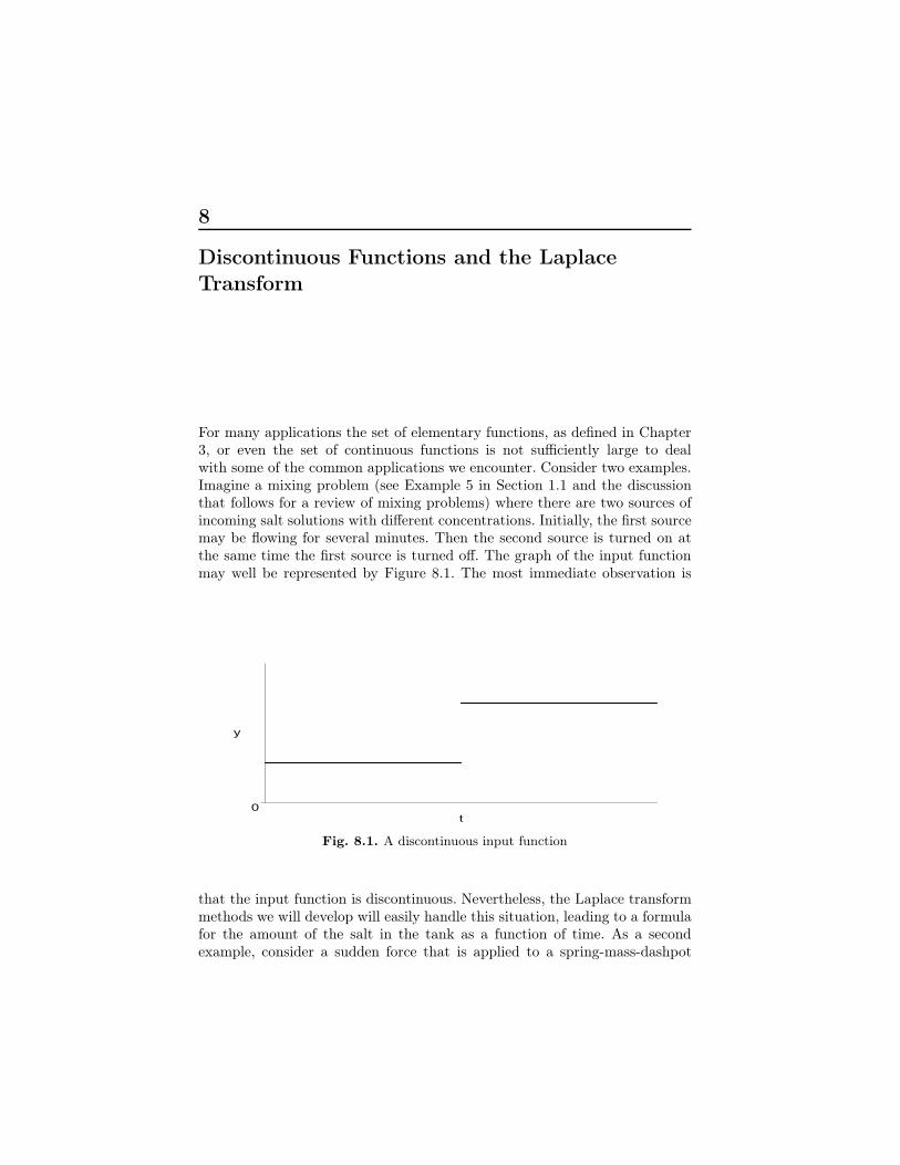
8
Discontinuous Functions and the Laplace
Transform
For many applications the set of elementary functions, as defined in Chapter3, or even the set of continuous functions is not sufficiently large to dealwith some of the common applications we encounter. Consider two examples.Imagine a mixing problem (see Example 5 in Section 1.1 and the discussionthat follows for a review of mixing problems) where there are two sources ofincoming salt solutions with different concentrations. Initially, the first sourcemay be flowing for several minutes. Then the second source is turned on atthe same time the first source is turned off. The graph of the input functionmay well be represented by Figure 8.1. The most immediate observation is
0
y
t
Fig. 8.1. A discontinuous input function
that the input function is discontinuous. Nevertheless, the Laplace transformmethods we will develop will easily handle this situation, leading to a formulafor the amount of the salt in the tank as a function of time. As a secondexample, consider a sudden force that is applied to a spring-mass-dashpot
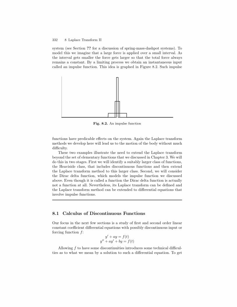
332 8 Laplace Transform II
system (see Section ?? for a discussion of spring-mass-dashpot systems). Tomodel this we imagine that a large force is applied over a small interval. Asthe interval gets smaller the force gets larger so that the total force alwaysremains a constant. By a limiting process we obtain an instantaneous inputcalled an impulse function. This idea is graphed in Figure 8.2. Such impulse
Fig. 8.2. An impulse function
functions have predicable effects on the system. Again the Laplace transformmethods we develop here will lead us to the motion of the body without muchdifficulty.
These two examples illustrate the need to extend the Laplace transformbeyond the set of elementary functions that we discussed in Chapter 3. We willdo this in two stages. First we will identify a suitably larger class of functions,the Heaviside class, that includes discontinuous functions and then extendthe Laplace transform method to this larger class. Second, we will considerthe Dirac delta function, which models the impulse function we discussedabove. Even though it is called a function the Dirac delta function is actuallynot a function at all. Nevertheless, its Laplace transform can be defined andthe Laplace transform method can be extended to differential equations thatinvolve impulse functions.
8.1 Calculus of Discontinuous Functions
Our focus in the next few sections is a study of first and second order linearconstant coefficient differential equations with possibly discontinuous input orforcing function f :
y′ + ay = f(t)y′′ + ay′ + by = f(t)
Allowing f to have some discontinuities introduces some technical difficul-ties as to what we mean by a solution to such a differential equation. To get
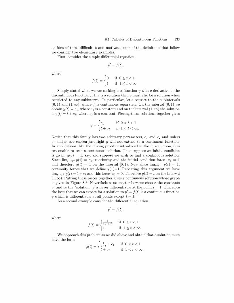
8.1 Calculus of Discontinuous Functions 333
an idea of these difficulties and motivate some of the definitions that followwe consider two elementary examples.
First, consider the simple differential equation
y′ = f(t),
where
f(t) =
0 if 0 ≤ t < 1
1 if 1 ≤ t <∞.Simply stated what we are seeking is a function y whose derivative is the
discontinuous function f . If y is a solution then y must also be a solution whenrestricted to any subinterval. In particular, let’s restrict to the subintervals(0, 1) and (1,∞), where f is continuous separately. On the interval (0, 1) weobtain y(t) = c1, where c1 is a constant and on the interval (1,∞) the solutionis y(t) = t+ c2, where c2 is a constant. Piecing these solutions together gives
y =
c1 if 0 < t < 1
t+ c2 if 1 < t <∞.
Notice that this family has two arbitrary parameters, c1 and c2 and unlessc1 and c2 are chosen just right y will not extend to a continuous function.In applications, like the mixing problem introduced in the introduction, it isreasonable to seek a continuous solution. Thus suppose an initial conditionis given, y(0) = 1, say, and suppose we wish to find a continuous solution.Since limt→0+ y(t) = c1, continuity and the initial condition forces c1 = 1and therefore y(t) = 1 on the interval [0, 1). Now since limt→1− y(t) = 1,continuity forces that we define y(1)=1. Repeating this argument we havelimt→1+ y(t) = 1+c2 and this forces c2 = 0. Therefore y(t) = t on the interval(1,∞). Putting these pieces together gives a continuous solution whose graphis given in Figure 8.3. Nevertheless, no matter how we choose the constantsc1 and c2 the "solution" y is never differentiable at the point t = 1. Thereforethe best that we can expect for a solution to y′ = f(t) is a continuous functiony which is differentiable at all points except t = 1.
As a second example consider the differential equation
y′ = f(t),
where
f(t) =
1(1−t)2 if 0 ≤ t < 1
1 if 1 ≤ t <∞.We approach this problem as we did above and obtain that a solution must
have the form
y(t) =
11−t + c1 if 0 < t < 1
t+ c2 if 1 < t <∞,
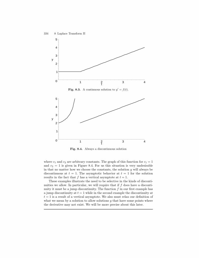
334 8 Laplace Transform II
0
1
2
3
4
5
y
1 2 3 4t
Fig. 8.3. A continuous solution to y′ = f(t).
0
1
2
3
4
5
y
1 2 3 4t
Fig. 8.4. Always a discontinuous solution
where c1 and c2 are arbitrary constants. The graph of this function for c1 = 1and c2 = 1 is given in Figure 8.4. For us this situation is very undesirablein that no matter how we choose the constants, the solution y will always bediscontinuous at t = 1. The asymptotic behavior at t = 1 for the solutionresults in the fact that f has a vertical asymptote at t = 1.
These examples illustrate the need to be selective in the kinds of disconti-nuities we allow. In particular, we will require that if f does have a disconti-nuity it must be a jump discontinuity. The function f in our first example hasa jump discontinuity at t = 1 while in the second example the discontinuity att = 1 is a result of a vertical asymptote. We also must relax our definition ofwhat we mean by a solution to allow solutions y that have some points wherethe derivative may not exist. We will be more precise about this later.
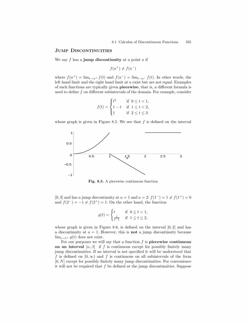
8.1 Calculus of Discontinuous Functions 335
Jump Discontinuities
We say f has a jump discontinuity at a point a if
f(a+) 6= f(a−)
where f(a+) = limt→a+ f(t) and f(a−) = limt→a− f(t). In other words, theleft hand limit and the right hand limit at a exist but are not equal. Examplesof such functions are typically given piecewise, that is, a different formula isused to define f on different subintervals of the domain. For example, consider
f(t) =
t2 if 0 ≤ t < 1,
1− t if 1 ≤ t < 2,
1 if 2 ≤ t ≤ 3
whose graph is given in Figure 8.5. We see that f is defined on the interval
–1
–0.5
0
0.5
1
0.5 1 1.5 2 2.5 3x
Fig. 8.5. A piecewise continuous function
[0, 3] and has a jump discontinuity at a = 1 and a = 2: f(1−) = 1 6= f(1+) = 0and f(2−) = −1 6= f(2+) = 1. On the other hand, the function
g(t) =
t if 0 ≤ t < 1,1
t−1 if 1 ≤ t ≤ 2,
whose graph is given in Figure 8.6, is defined on the interval [0, 2] and hasa discontinuity at a = 1. However, this is not a jump discontinuity becauselimt→1+ g(t) does not exist.
For our purposes we will say that a function f is piecewise continuouson an interval [α, β] if f is continuous except for possibly finitely manyjump discontinuities. If an interval is not specified it will be understood thatf is defined on [0,∞) and f is continuous on all subintervals of the form[0, N ] except for possibly finitely many jump discontinuities. For convenienceit will not be required that f be defined at the jump discontinuities. Suppose
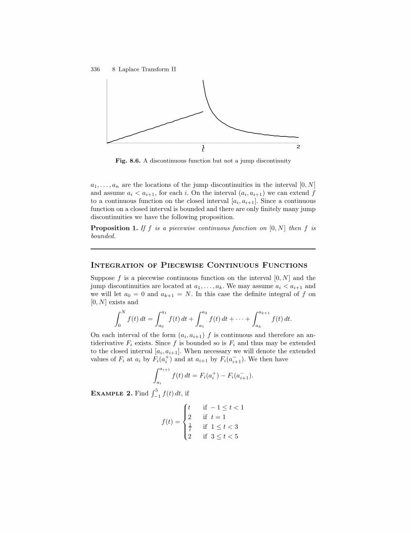
336 8 Laplace Transform II
1 2t
Fig. 8.6. A discontinuous function but not a jump discontinuity
a1, . . . , an are the locations of the jump discontinuities in the interval [0, N ]and assume ai < ai+1, for each i. On the interval (ai, ai+1) we can extend fto a continuous function on the closed interval [ai, ai+1]. Since a continuousfunction on a closed interval is bounded and there are only finitely many jumpdiscontinuities we have the following proposition.
Proposition 1. If f is a piecewise continuous function on [0, N ] then f isbounded.
Integration of Piecewise Continuous Functions
Suppose f is a piecewise continuous function on the interval [0, N ] and thejump discontinuities are located at a1, . . . , ak. We may assume ai < ai+1 andwe will let a0 = 0 and ak+1 = N . In this case the definite integral of f on[0, N ] exists and
∫ N
0
f(t) dt =
∫ a1
a0
f(t) dt+
∫ a2
a1
f(t) dt+ · · ·+∫ ak+1
ak
f(t) dt.
On each interval of the form (ai, ai+1) f is continuous and therefore an an-tiderivative Fi exists. Since f is bounded so is Fi and thus may be extendedto the closed interval [ai, ai+1]. When necessary we will denote the extendedvalues of Fi at ai by Fi(a
+i ) and at ai+1 by Fi(a
−i+1). We then have
∫ ai+1
ai
f(t) dt = Fi(a+i )− Fi(a
−i+1).
Example 2. Find∫ 5
−1 f(t) dt, if
f(t) =
t if − 1 ≤ t < 1
2 if t = 11t if 1 ≤ t < 3
2 if 3 ≤ t < 5
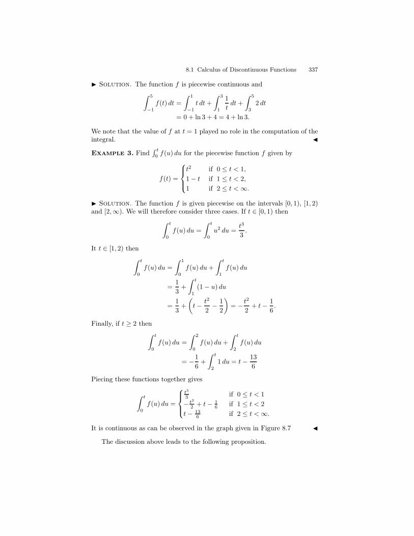
8.1 Calculus of Discontinuous Functions 337
I Solution. The function f is piecewise continuous and
∫ 5
−1
f(t) dt =
∫ 1
−1
t dt+
∫ 3
1
1
tdt+
∫ 5
3
2 dt
= 0 + ln 3 + 4 = 4 + ln 3.
We note that the value of f at t = 1 played no role in the computation of theintegral. J
Example 3. Find∫ t
0 f(u) du for the piecewise function f given by
f(t) =
t2 if 0 ≤ t < 1,
1− t if 1 ≤ t < 2,
1 if 2 ≤ t <∞.
I Solution. The function f is given piecewise on the intervals [0, 1), [1, 2)and [2,∞). We will therefore consider three cases. If t ∈ [0, 1) then
∫ t
0
f(u) du =
∫ t
0
u2 du =t3
3.
It t ∈ [1, 2) then
∫ t
0
f(u) du =
∫ 1
0
f(u) du+
∫ t
1
f(u) du
=1
3+
∫ t
1
(1− u) du
=1
3+
(
t− t2
2− 1
2
)
= − t2
2+ t− 1
6.
Finally, if t ≥ 2 then
∫ t
0
f(u) du =
∫ 2
0
f(u) du+
∫ t
2
f(u) du
= −1
6+
∫ t
2
1 du = t− 13
6
Piecing these functions together gives
∫ t
0
f(u) du =
t3
3 if 0 ≤ t < 1
− t2
2 + t− 16 if 1 ≤ t < 2
t− 136 if 2 ≤ t <∞.
It is continuous as can be observed in the graph given in Figure 8.7 J
The discussion above leads to the following proposition.
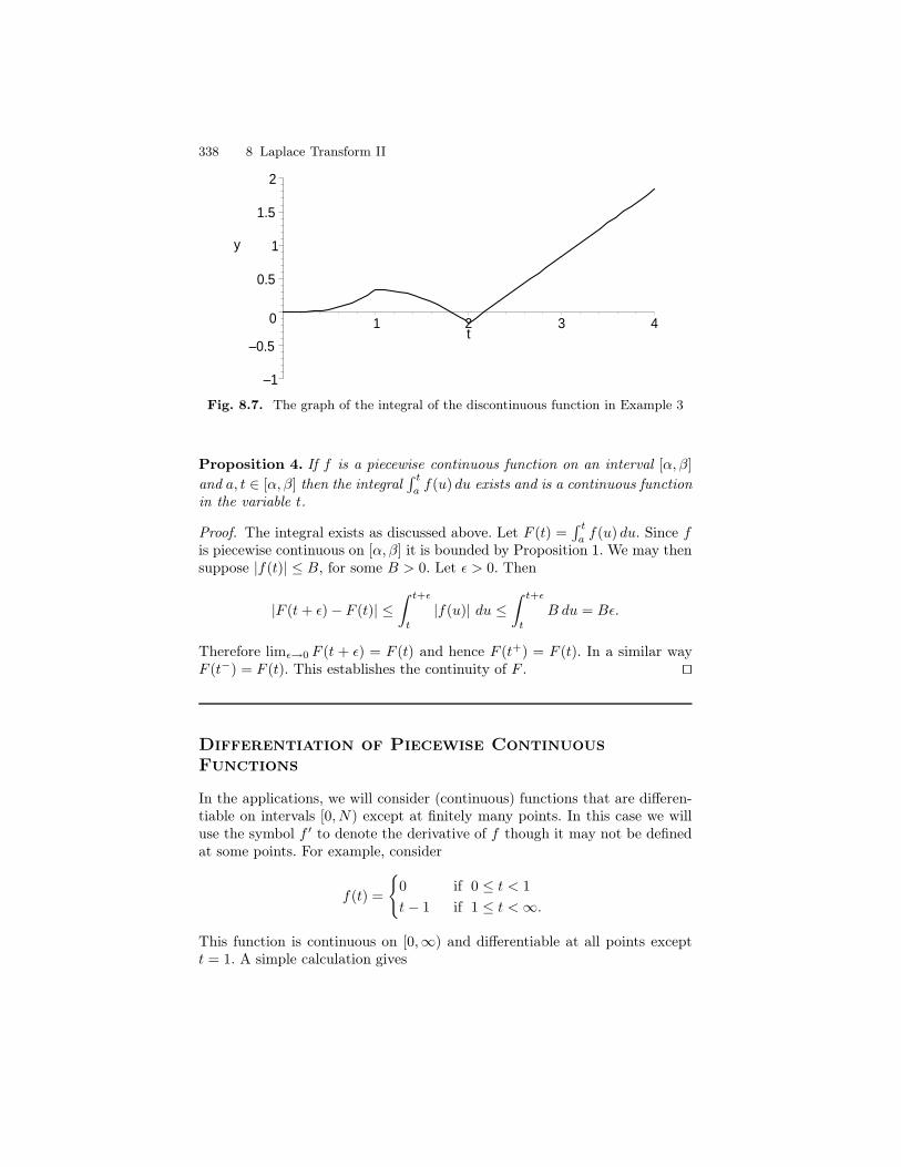
338 8 Laplace Transform II
–1
–0.5
0
0.5
1
1.5
2
y
1 2 3 4t
Fig. 8.7. The graph of the integral of the discontinuous function in Example 3
Proposition 4. If f is a piecewise continuous function on an interval [α, β]
and a, t ∈ [α, β] then the integral∫ t
a f(u) du exists and is a continuous functionin the variable t.
Proof. The integral exists as discussed above. Let F (t) =∫ t
a f(u) du. Since fis piecewise continuous on [α, β] it is bounded by Proposition 1. We may thensuppose |f(t)| ≤ B, for some B > 0. Let ε > 0. Then
|F (t+ ε)− F (t)| ≤∫ t+ε
t
|f(u)| du ≤∫ t+ε
t
B du = Bε.
Therefore limε→0 F (t + ε) = F (t) and hence F (t+) = F (t). In a similar wayF (t−) = F (t). This establishes the continuity of F . ut
Differentiation of Piecewise Continuous
Functions
In the applications, we will consider (continuous) functions that are differen-tiable on intervals [0, N) except at finitely many points. In this case we willuse the symbol f ′ to denote the derivative of f though it may not be definedat some points. For example, consider
f(t) =
0 if 0 ≤ t < 1
t− 1 if 1 ≤ t <∞.
This function is continuous on [0,∞) and differentiable at all points exceptt = 1. A simple calculation gives
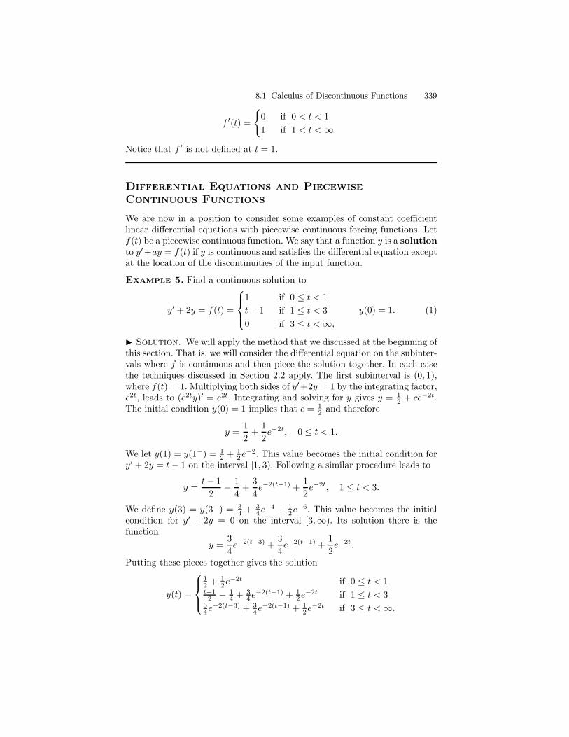
8.1 Calculus of Discontinuous Functions 339
f ′(t) =
0 if 0 < t < 1
1 if 1 < t <∞.
Notice that f ′ is not defined at t = 1.
Differential Equations and Piecewise
Continuous Functions
We are now in a position to consider some examples of constant coefficientlinear differential equations with piecewise continuous forcing functions. Letf(t) be a piecewise continuous function. We say that a function y is a solutionto y′+ay = f(t) if y is continuous and satisfies the differential equation exceptat the location of the discontinuities of the input function.
Example 5. Find a continuous solution to
y′ + 2y = f(t) =
1 if 0 ≤ t < 1
t− 1 if 1 ≤ t < 3
0 if 3 ≤ t <∞,y(0) = 1. (1)
I Solution. We will apply the method that we discussed at the beginning ofthis section. That is, we will consider the differential equation on the subinter-vals where f is continuous and then piece the solution together. In each casethe techniques discussed in Section 2.2 apply. The first subinterval is (0, 1),where f(t) = 1. Multiplying both sides of y′+2y = 1 by the integrating factor,e2t, leads to (e2ty)′ = e2t. Integrating and solving for y gives y = 1
2 + ce−2t.The initial condition y(0) = 1 implies that c = 1
2 and therefore
y =1
2+
1
2e−2t, 0 ≤ t < 1.
We let y(1) = y(1−) = 12 + 1
2e−2. This value becomes the initial condition for
y′ + 2y = t− 1 on the interval [1, 3). Following a similar procedure leads to
y =t− 1
2− 1
4+
3
4e−2(t−1) +
1
2e−2t, 1 ≤ t < 3.
We define y(3) = y(3−) = 34 + 3
4e−4 + 1
2e−6. This value becomes the initial
condition for y′ + 2y = 0 on the interval [3,∞). Its solution there is thefunction
y =3
4e−2(t−3) +
3
4e−2(t−1) +
1
2e−2t.
Putting these pieces together gives the solution
y(t) =
12 + 1
2e−2t if 0 ≤ t < 1
t−12 − 1
4 + 34e
−2(t−1) + 12e
−2t if 1 ≤ t < 334e
−2(t−3) + 34e
−2(t−1) + 12e
−2t if 3 ≤ t <∞.
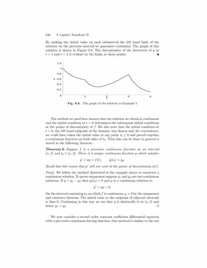
340 8 Laplace Transform II
By making the initial value on each subinterval the left hand limit of thesolution on the previous interval we guarantee continuity. The graph of thissolution is shown in Figure 8.8. The discontinuity of the derivative of y att = 1 and t = 3 is evident by the kinks at those points. J
0
0.2
0.4
0.6
0.8
1
1.2
y
1 2 3 4t
Fig. 8.8. The graph of the solution to Example 5
The method we used here insures that the solution we obtain is continuousand the initial condition at t = 0 determines the subsequent initial conditionsat the points of discontinuity of f . We also note that the initial condition att = 0, the left hand endpoint of the domain, was chosen only for convenience;we could have taken the initial value at any point t0 ≥ 0 and pieced togethera continuous function on both sides of t0. That this can be done in general isstated in the following theorem.
Theorem 6. Suppose f is a piecewise continuous function on an interval[α, β] and t0 ∈ [α, β]. There is a unique continuous function y which satisfies
y′ + ay = f(t), y(t0) = y0.
Recall that this means that y′ will not exist at the points of discontinuity of f .
Proof. We follow the method illustrated in the example above to construct acontinuous solution. To prove uniqueness suppose y1 and y2 are two continuoussolutions. If y = y1 − y2 then y(t0) = 0 and y is a continuous solution to
y′ + ay = 0.
On the interval containing t0 on which f is continuous, y = 0 by the uniquenessand existence theorem. The initial value at the endpoint of adjacent intervalsis thus 0. Continuing in this way we see that y is identically 0 on [α, β] andhence y1 = y2. ut
We now consider a second order constant coefficient differential equationwith a piecewise continuous forcing function. Our method is similar to the one
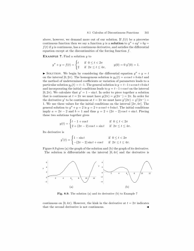
8.1 Calculus of Discontinuous Functions 341
above, however, we demand more out of our solution. If f(t) be a piecewisecontinuous function then we say a function y is a solution to y′′ + ay′ + by =f(t) if y is continuous, has a continuous derivative, and satisfies the differentialequation except at the discontinuities of the forcing function f .
Example 7. Find a solution y to
y′′ + y = f(t) =
t if 0 ≤ t < 2π
2 if 2π ≤ t ≤ 4π,y(0) = 0 y′(0) = 1.
I Solution. We begin by considering the differential equation y′′ + y = ton the interval [0, 2π). The homogenous solution is yh(t) = a cos t+ b sin t andthe method of undetermined coefficients or variation of parameters leads to aparticular solution yp(t) = t−1. The general solution is y = t−1+a cos t+b sin tand incorporating the initial conditions leads to y = t−1+cos t on the interval[0, 2π). We calculate that y′ = 1 − sin t. In order to piece together a solutionthat is continuous at t = 2π we must have y(2π) = y(2π−) = 2π. In order forthe derivative y′ to be continuous at t = 2π we must have y′(2π) = y′(2π−) =1. We use these values for the initial conditions on the interval [2π, 4π]. Thegeneral solution to y′′ + y = 2 is y = 2+ a cos t+ b sin t. The initial conditionsimply a = 2π − 2 and b = 1 and thus y = 2 + (2π − 2) cos t + sin t. Piecingthese two solutions together gives
y(t) =
t− 1 + cos t if 0 ≤ t < 2π
2 + (2π − 2) cos t+ sin t if 2π ≤ t ≤ 4π.
Its derivative is
y′(t) =
1− sin t if 0 ≤ t < 2π
−(2π − 2) sin t+ cos t if 2π ≤ t ≤ 4π.
Figure 8.9 gives (a) the graph of the solution and (b) the graph of its derivative.The solution is differentiable on the interval [0, 4π] and the derivative is
–2
0
2
4
6
y
2 4 6 8 10 12t
(a)
–4
–2
0
2
4
y
2 4 6 8 10 12t
(b)
Fig. 8.9. The solution (a) and its derivative (b) to Example 7
continuous on [0, 4π). However, the kink in the derivative at t = 2π indicatesthat the second derivative is not continuous. J
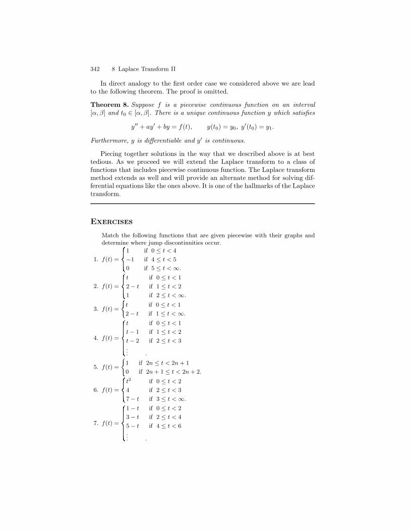
342 8 Laplace Transform II
In direct analogy to the first order case we considered above we are leadto the following theorem. The proof is omitted.
Theorem 8. Suppose f is a piecewise continuous function on an interval[α, β] and t0 ∈ [α, β]. There is a unique continuous function y which satisfies
y′′ + ay′ + by = f(t), y(t0) = y0, y′(t0) = y1.
Furthermore, y is differentiable and y′ is continuous.
Piecing together solutions in the way that we described above is at besttedious. As we proceed we will extend the Laplace transform to a class offunctions that includes piecewise continuous function. The Laplace transformmethod extends as well and will provide an alternate method for solving dif-ferential equations like the ones above. It is one of the hallmarks of the Laplacetransform.
Exercises
Match the following functions that are given piecewise with their graphs anddetermine where jump discontinuities occur.
1. f(t) = 1 if 0 ≤ t < 4
−1 if 4 ≤ t < 5
0 if 5 ≤ t < ∞.
2. f(t) = t if 0 ≤ t < 1
2 − t if 1 ≤ t < 2
1 if 2 ≤ t < ∞.
3. f(t) = t if 0 ≤ t < 1
2 − t if 1 ≤ t < ∞.
4. f(t) =t if 0 ≤ t < 1
t − 1 if 1 ≤ t < 2
t − 2 if 2 ≤ t < 3... .
5. f(t) = 1 if 2n ≤ t < 2n + 1
0 if 2n + 1 ≤ t < 2n + 2.
6. f(t) = t2 if 0 ≤ t < 2
4 if 2 ≤ t < 3
7 − t if 3 ≤ t < ∞.
7. f(t) =1 − t if 0 ≤ t < 2
3 − t if 2 ≤ t < 4
5 − t if 4 ≤ t < 6... .
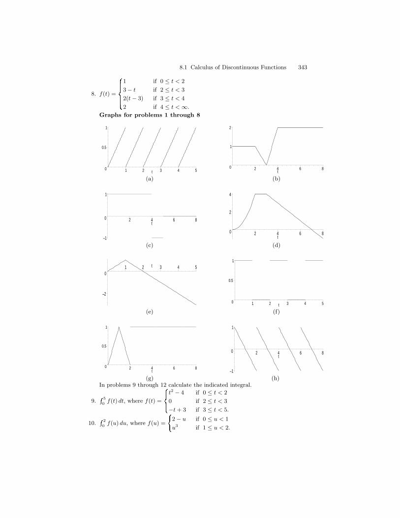
8.1 Calculus of Discontinuous Functions 343
8. f(t) =1 if 0 ≤ t < 2
3 − t if 2 ≤ t < 3
2(t − 3) if 3 ≤ t < 4
2 if 4 ≤ t < ∞.
Graphs for problems 1 through 8
0
0.5
1
1 2 3 4 5t0
1
2
2 4 6 8t
(a) (b)
–1
0
1
2 4 6 8t
0
2
4
2 4 6 8t
(c) (d)
–2
01 2 3 4 5t
0
0.5
1
1 2 3 4 5t
(e) (f)
0
0.5
1
2 4 6 8t –1
0
1
2 4 6 8t
(g) (h)In problems 9 through 12 calculate the indicated integral.
9. 5
0f(t) dt, where f(t) = t2 − 4 if 0 ≤ t < 2
0 if 2 ≤ t < 3
−t + 3 if 3 ≤ t < 5.
10. 2
0f(u) du, where f(u) = 2 − u if 0 ≤ u < 1
u3 if 1 ≤ u < 2.
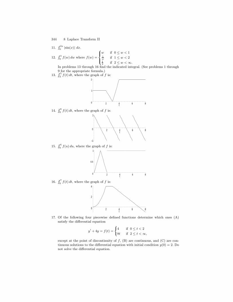
344 8 Laplace Transform II
11. 2π
0|sin(x)| dx.
12. 3
0f(w) dw where f(w) = w if 0 ≤ w < 1
1w
if 1 ≤ w < 212
if 2 ≤ w < ∞.In problems 13 through 16 find the indicated integral. (See problems 1 through9 for the appropriate formula.)
13. 5
2f(t) dt, where the graph of f is:
0
1
2
2 4 6 8t
14. 8
0f(t) dt, where the graph of f is:
–1
0
1
2 4 6 8t
15. 6
0f(u) du, where the graph of f is:
0
0.5
1
2 4 6 8t
16. 7
0f(t) dt, where the graph of f is:
0
2
4
2 4 6 8t
17. Of the following four piecewise defined functions determine which ones (A)satisfy the differential equation
y′ + 4y = f(t) = 4 if 0 ≤ t < 2
8t if 2 ≤ t < ∞,
except at the point of discontinuity of f , (B) are continuous, and (C) are con-tinuous solutions to the differential equation with initial condition y(0) = 2. Donot solve the differential equation.
8.1 Calculus of Discontinuous Functions 345
a) y(t) = 1 if 0 ≤ t < 2
2t − 12− 5
2e−4(t−2) if 2 ≤ t < ∞
b) y(t) = 1 + e−4t if 0 ≤ t < 2
2t − 12− 5
2e−4(t−2) + e−4t if 2 ≤ t < ∞
c) y(t) = 1 + e−4t if 0 ≤ t < 2
2t − 12− 5e−4(t−2)
2if 2 ≤ t < ∞
d) y(t) = 2e−4t if 0 ≤ t < 2
2t − 12− 5
2e−4(t−2) + e−4t if 2 ≤ t < ∞
18. Of the following four piecewise defined functions determine which ones (A)satisfy the differential equation
y′′ − 3y′ = 2y = f(t) = et if 0 ≤ t < 1
e2t if 1 ≤ t < ∞,
except at the point of discontinuity of f , (B) are continuous, and (C) have con-tinuous derivatives, and (D) are continuous solutions to the differential equationwith initial conditions y(0) = 0 and y′(0) = 0 and have continuous derivatives.Do not solve the differential equation.
a) y(t) = −tet − et + e2t if 0 ≤ t < 1
te2t − 2et if 1 ≤ t < ∞
b) y(t) = −tet − et + e2t if 0 ≤ t < 1
te2t − 3et − 12e2t if 1 ≤ t < ∞
c) y(t) = −tet − et + e2t if 0 ≤ t < 1
te2t + et+1 − et − e2t − e2t−1 if 1 ≤ t < ∞
d) y(t) = −tet + et − e2t if 0 ≤ t < 1
te2t + et+1 + et − e2t−1 − 3e2t if 1 ≤ t < ∞Solve the following differential equations.
19. y′ + 3y = t if 0 ≤ t < 1
1 if 1 ≤ t < ∞,y(0) = 0.
20. y′ − y =0 if 0 ≤ t < 1
t − 1 if 1 ≤ t < 2
3 − t if 2 ≤ t < 3
0 if 3 ≤ t < ∞,
y(0) = 0.
21. y′ + y = sin t if 0 ≤ t < π
0 if π ≤ t < ∞y(π) = −1.
22. y′′ − y = t if 0 ≤ t < 1
0 if 1 ≤ t < ∞,y(0) = 0, y′(0) = 1.
23. y′′ − 4y′ + 4y = 0 if 0 ≤ t < 2
4 if 2 ≤ t < ∞y(0) = 1, y′(0) = 0
24. Suppose f is a piecewise continuous function on an interval [α, β]. Let a ∈ [α, β]and define y(t) = y0 +
t
af(u) du. Show that y is a continuous solution to
y′ = f(t) y(a) = y0.
346 8 Laplace Transform II
25. Suppose f is a piecewise continuous function on an interval [α, β]. Let a ∈ [α, β]and define y(t) = y0 + e−at
t
aeauf(u) du. Show that y is a continuous solution
toy′ + ay = f(t) y(a) = y0.
26. Let f(t) = sin(1/t) if t 6= 0
0 if t = 0.
a) Show that f is bounded.b) Show that f is not continuous at t = 0.c) Show that f is not piecewise continuous.
8.2 The Heaviside class H
In this section we will extend the definition of the Laplace transform beyondthe set of elementary functions E to include piecewise continuous functions.The Laplace transform method will extend as well and provide a rather simplemeans of dealing with the differential equations we saw in Section 8.1.
Since the Laplace transform
Lf (s) =
∫ ∞
0
e−stf(t) dt
is defined by means of an improper integral, we must be careful about the issueof convergence. Recall that this definition means we compute
∫ N
0e−stf(t) dt
and then take the limit as N goes to infinity. To insure convergence we musttake into consideration the kinds of functions we feed into it. There are twomain reasons why such improper integrals may fail to exist. First, if the dis-tribution of the discontinuities of f is ‘too bad’ then even the finite integral∫ N
0e−stf(t) dt may fail to exist. Second, if the finite integral exists the limit
as N goes to ∞ may not. This has to do with how fast f grows. These twoissues will be handled separately by (1) identifying the particular type of dis-continuities allowed and (2) restricting the type of growth that f is allowed.What will result is a class of functions large enough to handle most of theapplications one is likely to encounter.
The first issue is handled for us by restricting to the piecewise continuousfunctions defined in section 8.1. If f is a piecewise continuous function (on[0,∞)) then so is t 7→ e−stf(t). By Proposition 4 the integral
∫ N
0
e−stf(t) dt
exists and is a continuous function in the variable N . Now to insure conver-gence as N goes to ∞ we must place a further requirement on f .
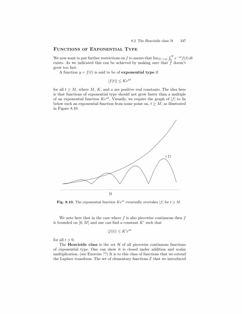
8.2 The Heaviside class H 347
Functions of Exponential Type
We now want to put further restrictions on f to assure that limN→∞∫ N
0 e−stf(t) dtexists. As we indicated this can be achieved by making sure that f doesn’tgrow too fast.
A function y = f(t) is said to be of exponential type if
|f(t)| ≤ Keat
for all t ≥ M , where M , K, and a are positive real constants. The idea hereis that functions of exponential type should not grow faster than a multipleof an exponential function Keat. Visually, we require the graph of |f | to liebelow such an exponential function from some point on, t ≥M , as illustratedin Figure 8.10.
M
_ f _
Fig. 8.10. The exponential function Keat eventually overtakes |f | for t ≥ M .
We note here that in the case where f is also piecewise continuous then fis bounded on [0,M ] and one can find a constant K ′ such that
|f(t)| ≤ K ′eat
for all t > 0.The Heaviside class is the set H of all piecewise continuous functions
of exponential type. One can show it is closed under addition and scalarmultiplication. (see Exercise ??) It is to this class of functions that we extendthe Laplace transform. The set of elementary functions E that we introduced
348 8 Laplace Transform II
in Chapter 3 are all examples of functions in the Heaviside class. Recall thatf is an elementary function if f is a sum of functions of the form ctneat sin(bt)and ctneat cos(bt), where a, b, c are constants and n is a nonnegative integer.Such functions are continuous. Since sin and cos are bounded by 1 and tn ≤ ent
it follows that |ctneat sin bt| ≤ ce(a+n)t and likewise |ctneat cos bt| ≤ ce(a+n)t.Thus elementary functions are of exponential type, i.e., E ⊂ H. Although theHeaviside class is much bigger than the set of elementary functions there aremany important functions which are not in H. An example is f(t) = et2 . Forif b is any positive constant, then
et2
ebt= et2−bt = e(t−
b2 )2− b2
4
and therefore,
limt→∞
et2
ebt=∞.
This implies that f(t) = et2 grows faster than any exponential function andthus is not of exponential type.
Existence of the Laplace transform
Recall that for an elementary function the Laplace transform exists and hasthe further property that lims→∞ F (s) = 0. These two properties extend toall functions in the Heaviside class.
Theorem 1. For f ∈ H the Laplace transform exists and
lims→∞
F (s) = 0.
Proof. The finite integral∫ N
0e−stf(t) dt exists because f is piecewise contin-
uous on [0, N ]. Since f is also of exponential type there are constants K anda such that |f(t)| ≤ Keat for all t ≥ 0. Thus, for all s > a,
∫ ∞
0
|e−stf(t)| dt ≤∫ ∞
0
|e−stKeat| dt
= K
∫ ∞
0
e−(s−a)t dt
=K
s− a .
This shows that the integral converges absolutely and hence the Laplace trans-form exists for s > a. Since |L f (s)| ≤ K
s−a and lims→∞K
s−a = 0 it followsthat
lims→∞
Lf (s) = 0.
ut
8.2 The Heaviside class H 349
As might be expected computations using the definition to computeLaplace transforms of even simple functions can be tedious. To illustrate thepoint consider the following example.
Example 2. Use the definition to compute the Laplace transform of
f(t) =
t2 if 0 ≤ t < 1
2 if 1 ≤ t <∞.
I Solution. Clearly f is piecewise continuous and bounded, hence it is inthe Heaviside class. We can thus proceed with the definition confident, byTheorem 1, that the improper integral will converge. We have
Lf (s) =
∫ ∞
0
e−stf(t) dt
=
∫ 1
0
e−st t2 dt+
∫ ∞
1
e−st 2 dt
For the first integral we need integration by parts twice:
∫ 1
0
e−st t2 dt =t2e−st
−s |10 +
2
s
∫ 1
0
e−st t dt
=e−s
−s +2
s
(
te−st
−s |10 +
1
s
∫ 1
0
e−st dt
)
= −e−s
s+
2
s
(
−e−s
s− 1
s2e−st|10
)
= −e−s
s− 2e−s
s2+
2
s3− 2e−s
s3.
The second integral is much simpler and we get
∫ ∞
1
e−st 2 dt =2e−s
s
Now putting things together and simplifying gives
Lf (s) =2
s3+ e−s
(
− 2
s3− 2
s2+
1
s
)
.
J
Do not despair. The Heaviside function that we introduce next will leadto a Laplace transform principle that will make unnecessary calculations likethe one above.
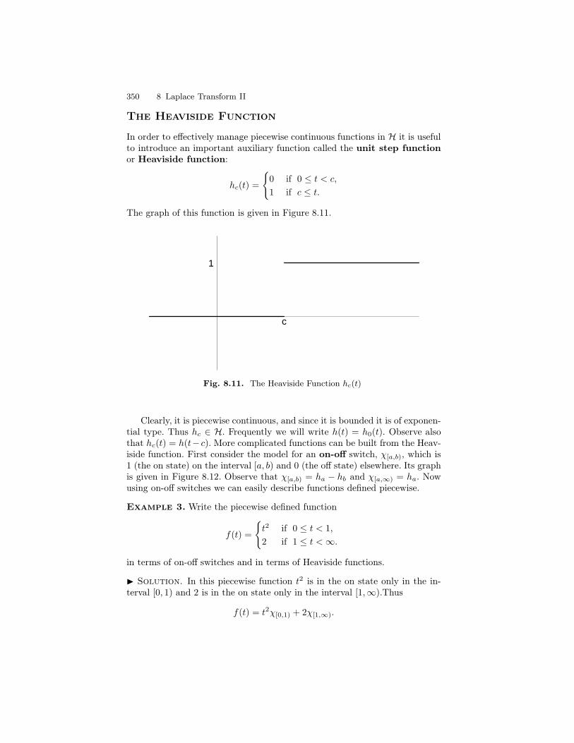
350 8 Laplace Transform II
The Heaviside Function
In order to effectively manage piecewise continuous functions in H it is usefulto introduce an important auxiliary function called the unit step functionor Heaviside function:
hc(t) =
0 if 0 ≤ t < c,
1 if c ≤ t.
The graph of this function is given in Figure 8.11.
1
c
Fig. 8.11. The Heaviside Function hc(t)
Clearly, it is piecewise continuous, and since it is bounded it is of exponen-tial type. Thus hc ∈ H. Frequently we will write h(t) = h0(t). Observe alsothat hc(t) = h(t− c). More complicated functions can be built from the Heav-iside function. First consider the model for an on-off switch, χ[a,b), which is1 (the on state) on the interval [a, b) and 0 (the off state) elsewhere. Its graphis given in Figure 8.12. Observe that χ[a,b) = ha − hb and χ[a,∞) = ha. Nowusing on-off switches we can easily describe functions defined piecewise.
Example 3. Write the piecewise defined function
f(t) =
t2 if 0 ≤ t < 1,
2 if 1 ≤ t <∞.
in terms of on-off switches and in terms of Heaviside functions.
I Solution. In this piecewise function t2 is in the on state only in the in-terval [0, 1) and 2 is in the on state only in the interval [1,∞).Thus
f(t) = t2χ[0,1) + 2χ[1,∞).
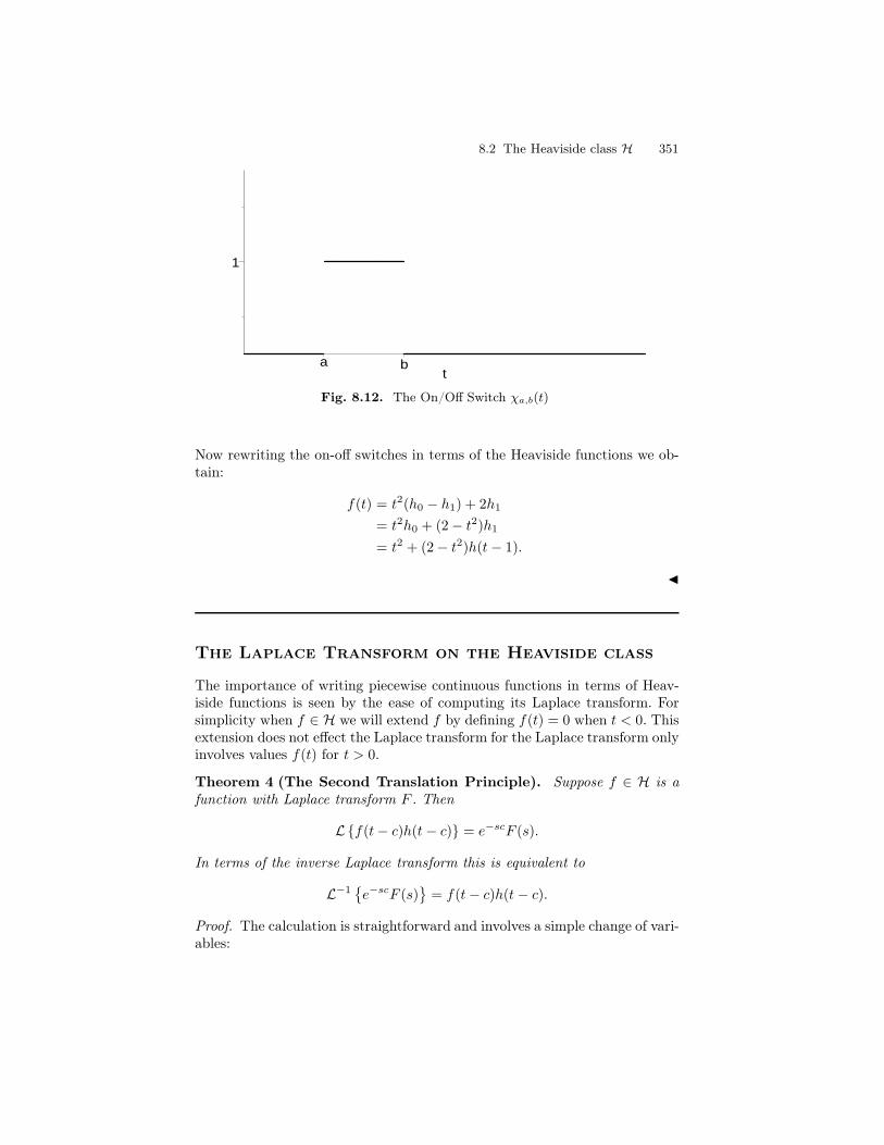
8.2 The Heaviside class H 351
1
a bt
Fig. 8.12. The On/Off Switch χa,b(t)
Now rewriting the on-off switches in terms of the Heaviside functions we ob-tain:
f(t) = t2(h0 − h1) + 2h1
= t2h0 + (2− t2)h1
= t2 + (2− t2)h(t− 1).
J
The Laplace Transform on the Heaviside class
The importance of writing piecewise continuous functions in terms of Heav-iside functions is seen by the ease of computing its Laplace transform. Forsimplicity when f ∈ H we will extend f by defining f(t) = 0 when t < 0. Thisextension does not effect the Laplace transform for the Laplace transform onlyinvolves values f(t) for t > 0.
Theorem 4 (The Second Translation Principle). Suppose f ∈ H is afunction with Laplace transform F . Then
Lf(t− c)h(t− c) = e−scF (s).
In terms of the inverse Laplace transform this is equivalent to
L−1
e−scF (s)
= f(t− c)h(t− c).
Proof. The calculation is straightforward and involves a simple change of vari-ables:
352 8 Laplace Transform II
Lf(t− c)h(t− c) (s) =
∫ ∞
0
e−stf(t− c)h(t− c) dt
=
∫ ∞
c
e−stf(t− c) dt
=
∫ ∞
0
e−s(t+c)f(t) dt (t 7→ t+ c)
= e−sc
∫ ∞
0
e−stf(t) dt
= e−scF (s)
ut
Frequently, we encounter expressions in the form g(t)h(t−c). If f(t) is replacedby g(t+ c) in Theorem 4 then we obtain
Corollary 5.Lg(t)h(t− c) = e−scLg(t+ c) .
A simple example of this is when g = 1. Then Lhc = e−scL1 = e−sc
s .When c = 0 then Lh0) = 1
s which is the same as the Laplace transform ofthe constant function 1. This is consistent since h0 = h = 1 for t ≥ 0.
Example 6. Find the Laplace transform of f(t) =
t2 if 0 ≤ t < 1
2 if 1 ≤ t <∞given in Example 8.2.
I Solution. In Example 3 we found f(t) = t2 + (2 − t2)h(t − 1). By theCorollary we get
Lf =2
s3+ e−sL
2− (t+ 1)2
=2
s3+ e−sL
−t2 − 2t+ 1
=2
s3+ e−s
(
− 2
s3− 2
s2+
1
s
)
J
Example 7. Find the Laplace transform of
f(t) =
cos t if 0 ≤ t < π
1 if π ≤ t < 2π
0 if 2π ≤ t <∞.
I Solution. First writing f in terms of on-off switches gives
f = cos t χ[0,π) + 1 χ[π,2π) + 0 χ[2π,∞).
8.2 The Heaviside class H 353
Now rewrite this expression in terms of Heaviside functions:
f = cos t (h0 − hπ) + (hπ − h2π) = cos t+ (1− cos t)hπ − h2π.
Since hc(t) = h(t− c) the corollary gives
F (s) =s
s2 + 1+ e−sπL1− cos(t+ π) − e−2sπ
s
=s
s2 + 1+ e−sπ
(
1
s+
s
s2 + 1
)
− e−2sπ
s.
In the second line we have used the fact that cos(t+ π) = − cos t. J
Exercises
Graph each of the following functions defined by means of the unit step functionh(t − c) and/or the on-off switches χ[a, b).
1. f(t) = 3h(t − 2) − h(t − 5)2. f(t) = 2h(t − 2) − 3h(t − 3) + 4h(t − 4)3. f(t) = (t − 1)h(t − 1)4. f(t) = (t − 2)2h(t − 2)5. f(t) = t2h(t − 2)6. f(t) = h(t − π) sin t7. f(t) = h(t − π) cos 2(t − π)8. f(t) = t2χ[0, 1) + (1 − t)χ[1, 3) + 3χ[3, ∞)
For each of the following functions f(t), (a) express f(t) in terms of on-off switches,(b) express f(t) in terms of Heaviside functions, and (c) compute the Laplace trans-form F (s) = Lf(t).
9. f(t) = 0 if 0 ≤ t < 2,
t − 2 if 2 ≤ t < ∞.
10. f(t) = 0 if 0 ≤ t < 2,
t if 2 ≤ t < ∞.
11. f(t) = 0 if 0 ≤ t < 2,
t + 2 if 2 ≤ t < ∞.
12. f(t) = 0 if 0 ≤ t < 4,
(t − 4)2 if 4 ≤ t < ∞.
13. f(t) = 0 if 0 ≤ t < 4,
t2 if 4 ≤ t < ∞.
14. f(t) = 0 if 0 ≤ t < 4,
t2 − 4 if 4 ≤ t < ∞.
354 8 Laplace Transform II
15. f(t) = 0 if 0 ≤ t < 2,
(t − 4)2 if 2 ≤ t < ∞.
16. f(t) = 0 if 0 ≤ t < 4,
et−4 if 4 ≤ t < ∞.
17. f(t) = 0 if 0 ≤ t < 4,
et if 4 ≤ t < ∞.
18. f(t) = 0 if 0 ≤ t < 6,
et−4 if 6 ≤ t < ∞.
19. f(t) = 0 if 0 ≤ t < 4,
tet if 4 ≤ t < ∞.
20. f(t) = 1 if 0 ≤ t < 4
−1 if 4 ≤ t < 5
0 if 5 ≤ t < ∞.
21. f(t) = t if 0 ≤ t < 1
2 − t if 1 ≤ t < 2
1 if 2 ≤ t < ∞.
22. f(t) = t if 0 ≤ t < 1
2 − t if 1 ≤ t < ∞.
23. f(t) =t if 0 ≤ t < 1
t − 1 if 1 ≤ t < 2
t − 2 if 2 ≤ t < 3... .
24. f(t) = 1 if 2n ≤ t < 2n + 1
0 if 2n + 1 ≤ t < 2n + 2.
25. f(t) = t2 if 0 ≤ t < 2
4 if 2 ≤ t < 3
7 − t if 3 ≤ t < ∞.
26. f(t) =1 − t if 0 ≤ t < 2
3 − t if 2 ≤ t < 4
5 − t if 4 ≤ t < 6... .
27. f(t) =1 if 0 ≤ t < 2
3 − t if 2 ≤ t < 3
2(t − 3) if 3 ≤ t < 4
2 if 4 ≤ t < ∞.
8.3 The Inversion of the Laplace Transform
We now turn our attention to the inversion of the Laplace transform. InChapter 3 we established a one-to-one correspondence between elementary
8.3 The Inversion of the Laplace Transform 355
functions and proper rational functions: for each proper rational function itsinverse Laplace transform is a unique elementary function. For the Heavisideclass the matter is complicated by our allowing discontinuity. Two functionsf1 and f2 are said to be essentially equal if for each interval [0, N) they areequal as functions except at possibly finitely many points. For example, thefunctions
f1(t) =
1 if 0 ≤ t < 1
2 if 1 ≤ t <∞ f2(t) =
1 if 0 ≤ t < 1
3 if t = 1
2 if 1 < t <∞f3(t) =
1 if 0 ≤ t ≤ 1
2 if 1 < t <∞.
are essentially equal for they are equal everywhere except at t = 1. Twofunctions that are essentially equal have the same Laplace transform. This isbecause the Laplace transform is an integral operator and integration cannotdistinguish functions that are essentially equal. The Laplace transform of f1,f2, and f3 in our example above are all 1
s + e−s
s . Here is our problem: Given a
transform, like 1s + e−s
s , how do we decide what ‘the’ inverse Laplace transformis. It turns out that if F (s) is the Laplace transform of functions f1, f2 ∈ Hthen f1 and f2 are essentially equal. For most practical situations it does notmatter which one is chosen. However, in this text we will consistently use theone that is right continuous at each point. A function f in the Heaviside classis said to be right continuous at a point a if we have
f(a) = f(a+) = limt→a+
f(t),
and it is right continuous on [0,∞) if it is right continuous at each pointin [0,∞). In the example above, f1 is right continuous while f2 and f3 are not.The function f3 is, however, left continuous, using the obvious definition ofleft continuity. If we decide to use right continuous functions in the Heavisideclass then the correspondence with its Laplace transform is one-to-one. Wesummarize this discussion as a theorem:
Theorem 1. If F (s) is the Laplace transform of a function in H then thereis a unique right continuous function f ∈ H such that Lf = F . Any twofunctions in H with the same Laplace transform are essentially equal.
Recall from our definition that hc is right continuous. So piecewise func-tions written as sums of products of a continuous function and a Heavisidefunction are right continuous.
Example 2. Find the inverse Laplace transform of
F (s) =e−s
s2+e−3s
s− 4
and write it as a right continuous piecewise function.
356 8 Laplace Transform II
I Solution. The inverse Laplace transforms of 1s2 and 1
s−4 are, respectively,t and e4t. By Theorem 4 the inverse Laplace transform of F (s) is
(t− 1)h1 + e4(t−3)h3.
On the interval [0, 1) both t− 1 and e4(t−3) are off. On the interval [1, 3) onlyt− 1 is on. On the interval [3,∞) both t− 1 and e4(t−3) are on. Thus
L−1 F (s) =
0 if 0 ≤ t < 1
t− 1 if 1 ≤ t < 3
t− 1 + e4(t−3) if 3 ≤ t <∞.
J
The Laplace Transform of tα and the Gamma
function
We showed in Chapter 3 that the Laplace transform of tn is n!sn+1 , for each
nonnegative integer n. One might conjecture that the Laplace transform oftα, for α an arbitrary nonnegative real number, is given by a similar formula.Such a formula would necessarily extend the notion of ‘factorial’. We definethe gamma function by the formula
Γ (α) =
∫ ∞
0
e−ttα−1 dt.
It can be shown that the improper integral that defines the gamma functionconverges as long as α is greater than 0. The following proposition, whose proofis left as an exercise, establishes the fundamental properties of the gammafunction.
Proposition 3.1. Γ (α+ 1) = αΓ (α) (The fundamental recurrence relation)2. Γ (1) = 13. Γ (n+ 1) = n!
The third formula in the proposition allows us to rewrite the Laplace transformof tn in the following way:
Ltn =Γ (n+ 1)
sn+1.
If α > −1 we obtain
Ltα =Γ (α+ 1)
sα+1.
8.3 The Inversion of the Laplace Transform 357
(Even though tα is not in the Heaviside class for −1 < α < 0 its Laplacetransform still exists.) To establish this formula fix α > −1. By definition
Ltα =
∫ ∞
0
e−sttα dt.
We make the change of variable u = st. Then du = sdt and
Ltα (s) =
∫ ∞
0
e−uu
s
du
s
=1
sα+1
∫ ∞
0
e−uuα du
=Γ (α+ 1)
sα+1.
Of course, in order to actually compute the Laplace transform of some noninteger positive power of t one must know the value of the gamma functionfor the corresponding power. For example, it is known that Γ (1
2 ) =√π. By
the fundamental recurrence relation Γ (32 ) = 1
2Γ (12 ) =
√π
2 . Therefore
L
t12
=
√π
2s32
.
Exercises
Compute the inverse Laplace transform of each of the following functions.
1.e−3s
s − 1
2.e−3s
s2
3.e−3s
(s − 1)3
4.e−πs
s2 + 1
5.se−3πs
s2 + 1
6.e−πs
s2 + 2s + 5
7.e−s
s2+
e−2s
(s − 1)3
8.e−2s
s2 + 4
9.e−2s
s2 − 4
10.se−4s
s2 + 3s + 2
358 8 Laplace Transform II
11.e−2s + e−3s
s2 − 3s + 2
12.1 − e−5s
s2
13.1 + e−3s
s4
14. e−πs 2s + 1
s2 + 6s + 13
15. 1 − e−πs 2s + 1
s2 + 6s + 13
8.4 Properties of the Laplace Transform
Many of the properties of the Laplace transform that we discussed in Chapter3 for elementary functions carry over to the Heaviside class. Their proofs arethe same. These properties are summarized below.
Linearity Laf + bg = aLf+ bLg .
The First Translation Principle Le−atf = Lf (s− a).
Differentiation in Transform Space L(−tf(t)) = F ′(s)L(−t)nf(t) = F (n)(s).
Integration in Domain Space L(
∫ t
0 f(u) du
= F (s)s .
There are a few properties though that need some clarifications. In partic-ular, we need to discuss the meaning of the fundamental derivative formula
Lf ′ = sLf − f(0),
when f is in the Heaviside class. You will recall that the derivative of an ele-mentary function is again an elementary function. However, for the Heavisideclass this is not necessarily the case. A couple of things can go wrong. First,there are examples of functions in H for which the derivative does not existat any point. Second, even when the derivative exists there is no guaranteethat it is back in H. As an example, consider the function
f(t) = sin et2 .
This function is in H because it is bounded (between −1 and 1) and contin-uous. However, its derivative is
f ′(t) = 2tet2 cos et2 ,
which is continuous but not of exponential type. To see this recall that et2 isnot of exponential type. Thus at those values of t where cos et2 = 1, |f ′(t)| is
8.4 Properties of the Laplace Transform 359
not bounded by an exponential function and hence f ′ /∈ H. Therefore, in orderto extend the derivative formula to H we must include in the hypotheses therequirement that both f and f ′ be in H. Recall that for f in H the symbolf ′ is used to denote the derivative of f if f is differentiable except at a finitenumber of points on each interval of the form [0, N ].
The Laplace Transform of a Derivative
With these understandings we now have
Theorem 1. If f is continuous and f and f ′ are in H then
Lf ′ = sLf − f(0).
Proof. We begin by computing∫ N
0 e−stf ′(t) dt. This integral requires that weconsider the points where f ′ is discontinuous. There are only finitely manyon [0, N), a1, . . . , ak, say, and we may assume ai < ai+1. If we et a0 = 0 andak+1 = N then we obtain
∫ N
0
e−stf ′(t) dt =
k∑
i=0
∫ ai+1
ai
e−stf ′(t) dt,
and integration by parts gives
∫ N
0
e−stf ′(t) dt =
k∑
i=0
(
f(t)e−st|ai+1ai
+ s
∫ ai+1
ai
e−stf(t) dt
)
=
k∑
i=0
(f(a−i+1)e−sai+1 − f(a+
i )e−sai) +
∫ N
0
e−stf(t) dt
= f(N)e−Ns − f(0) + s
∫ N
0
e−stf(t) dt.
We have used the continuity of f to make the evaluations at ai and ai+1,which allows for the collapsing sum in line 2. We now take the limit as N goesto infinity and the result follows. ut
The following corollary is immediate:
Corollary 2. If f and f ′ are continuous and f , f ′, and f ′′ are in H then
Lf ′′ = s2Lf − sf(0)− f ′(0).
360 8 Laplace Transform II
The Laplace Transform Method
The differential equations that we will solve by means of the Laplace transformare first and second order constant coefficient linear differential equations witha forcing function f in H:
y′ + ay = f(t)y′′ + ay′ + by = f(t).
In order to apply the Laplace transform method we will need to knowthat there is a solution y which is continuous in the first equation and bothy and y′ are continuous in the second equation. These facts were proved inTheorems 6 and 8.
We are now in a position to illustrate the Laplace transform method tosolve differential equations with possibly discontinuous forcing functions f .
Example 3. Solve the following first order differential equation:
y′ + 2y = f(t), y(0) = 1,
where
f(t) =
0 if 0 ≤ t < 1
t if 1 ≤ t <∞.
I Solution. We first rewrite f in terms of Heaviside functions: f(t) =t χ[1,∞)(t) = t h1(t). By Corollary 5 its Laplace transform is F (s) = e−sLt+ 1 =
e−s( 1s2 + 1
s ) = e−s( s+1s2 ). The Laplace transform of the differential equation
yields
sY (s)− y(0) + 2Y (s) = e−s(s+ 1
s2),
and solving for Y gives
Y (s) =1
s+ 2+ e−s s+ 1
s2(s+ 2).
A partial fraction decomposition gives
s+ 1
s2(s+ 2)=
1
4
1
s+
1
2
1
s2− 1
4
1
s+ 2,
and the second translation principle (Theorem 4) gives
y(t) = L−1
1
s+ 2
+1
4L−1
e−s 1
s
+1
2L−1
e−s 1
s2
− 1
4L−1
e−s 1
s+ 2
= e−2t +1
4h1 +
1
2(t− 1)h1 −
1
4e−2(t−1)h1.
=
e−2t if 0 ≤ t < 1
e−2t + 14 (2t− 1)− 1
4e−2(t−1) if 1 ≤ t <∞.
J
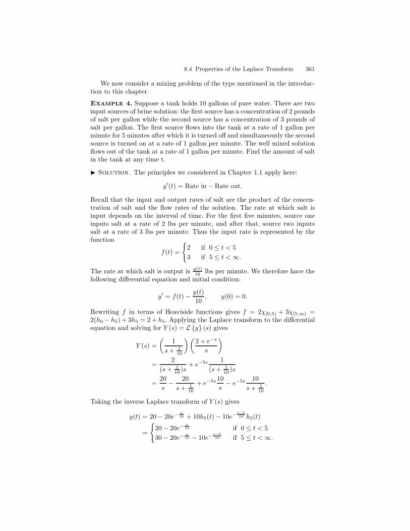
8.4 Properties of the Laplace Transform 361
We now consider a mixing problem of the type mentioned in the introduc-tion to this chapter.
Example 4. Suppose a tank holds 10 gallons of pure water. There are twoinput sources of brine solution: the first source has a concentration of 2 poundsof salt per gallon while the second source has a concentration of 3 pounds ofsalt per gallon. The first source flows into the tank at a rate of 1 gallon perminute for 5 minutes after which it is turned off and simultaneously the secondsource is turned on at a rate of 1 gallon per minute. The well mixed solutionflows out of the tank at a rate of 1 gallon per minute. Find the amount of saltin the tank at any time t.
I Solution. The principles we considered in Chapter 1.1 apply here:
y′(t) = Rate in− Rate out.
Recall that the input and output rates of salt are the product of the concen-tration of salt and the flow rates of the solution. The rate at which salt isinput depends on the interval of time. For the first five minutes, source oneinputs salt at a rate of 2 lbs per minute, and after that, source two inputssalt at a rate of 3 lbs per minute. Thus the input rate is represented by thefunction
f(t) =
2 if 0 ≤ t < 5
3 if 5 ≤ t <∞.
The rate at which salt is output is y(t)10 lbs per minute. We therefore have the
following differential equation and initial condition:
y′ = f(t)− y(t)
10, y(0) = 0.
Rewriting f in terms of Heaviside functions gives f = 2χ[0,5) + 3χ[5,∞) =2(h0 − h5) + 3h5 = 2 + h5. Applying the Laplace transform to the differentialequation and solving for Y (s) = Ly (s) gives
Y (s) =
(
1
s+ 110
)(
2 + e−s
s
)
=2
(s+ 110 )s
+ e−5s 1
(s+ 110 )s
=20
s− 20
s+ 110
+ e−5s 10
s− e−5s 10
s+ 110
.
Taking the inverse Laplace transform of Y (s) gives
y(t) = 20− 20e−t10 + 10h5(t)− 10e−
t−510 h5(t)
=
20− 20e−t10 if 0 ≤ t < 5
30− 20e−t10 − 10e−
t−510 if 5 ≤ t <∞.
362 8 Laplace Transform II
The graph of y is given in Figure 8.13. As expected we observe that thesolution is continuous, but the small kink at t = 5 indicates that there is adiscontinuity of the derivative at this point. This occurred when the flow ofthe second source, which had a higher concentration of salt, was turned on.
J
0
5
10
15
20
25
30
10 20 30 40 50t
Fig. 8.13. The solution to a mixing problem with discontinuous input function.
Exercises
Solve each of the following initial value problems.
1. y′ + 2y = f(t) where f(t) = 0 if 0 ≤ t < 1
−3 if t ≥ 1y(0) = 0.
2. y′ + 2y = f(t) where f(t) = −2 if 0 ≤ t < 1
2 if t ≥ 1y(0) = 0.
3. y′ + 2y = f(t) where f(t) = 0 if 0 ≤ t < 1
2 if 1 ≤ t < 3
0 if t ≥ 3
y(0) = 0.
4. y′ + 2y = f(t) where f(t) = t if 0 ≤ t < 1
0 if t ≥ 1y(0) = 0.
5. y′′ + 9y = h(t − 3), y(0) = 0, y′(0) = 0.
6. y′′ − 5y′ + 4y = f(t) where f(t) = 1 if 0 ≤ t < 5
0 if t ≥ 5y(0) = 0, y′(0) = 1.
7. y′′ + 5y′ + 6y = 0 if 0 ≤ t < 1
2 if 1 ≤ t < 3
0 if t ≥ 3
y(0) = 0, y′(0) = 0.
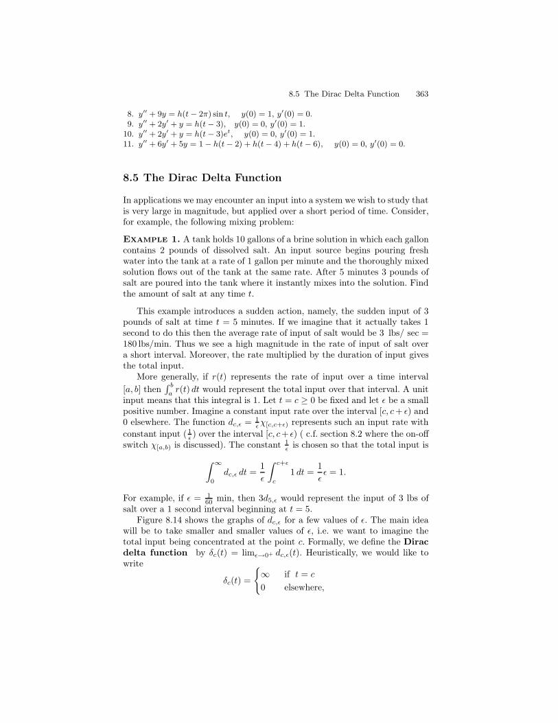
8.5 The Dirac Delta Function 363
8. y′′ + 9y = h(t − 2π) sin t, y(0) = 1, y′(0) = 0.9. y′′ + 2y′ + y = h(t − 3), y(0) = 0, y′(0) = 1.
10. y′′ + 2y′ + y = h(t − 3)et, y(0) = 0, y′(0) = 1.11. y′′ + 6y′ + 5y = 1 − h(t − 2) + h(t − 4) + h(t − 6), y(0) = 0, y′(0) = 0.
8.5 The Dirac Delta Function
In applications we may encounter an input into a system we wish to study thatis very large in magnitude, but applied over a short period of time. Consider,for example, the following mixing problem:
Example 1. A tank holds 10 gallons of a brine solution in which each galloncontains 2 pounds of dissolved salt. An input source begins pouring freshwater into the tank at a rate of 1 gallon per minute and the thoroughly mixedsolution flows out of the tank at the same rate. After 5 minutes 3 pounds ofsalt are poured into the tank where it instantly mixes into the solution. Findthe amount of salt at any time t.
This example introduces a sudden action, namely, the sudden input of 3pounds of salt at time t = 5 minutes. If we imagine that it actually takes 1second to do this then the average rate of input of salt would be 3 lbs/ sec =180 lbs/min. Thus we see a high magnitude in the rate of input of salt overa short interval. Moreover, the rate multiplied by the duration of input givesthe total input.
More generally, if r(t) represents the rate of input over a time interval[a, b] then
∫ b
ar(t) dt would represent the total input over that interval. A unit
input means that this integral is 1. Let t = c ≥ 0 be fixed and let ε be a smallpositive number. Imagine a constant input rate over the interval [c, c+ ε) and0 elsewhere. The function dc,ε = 1
εχ[c,c+ε) represents such an input rate withconstant input (1
ε ) over the interval [c, c+ ε) ( c.f. section 8.2 where the on-offswitch χ[a,b) is discussed). The constant 1
ε is chosen so that the total input is
∫ ∞
0
dc,ε dt =1
ε
∫ c+ε
c
1 dt =1
εε = 1.
For example, if ε = 160 min, then 3d5,ε would represent the input of 3 lbs of
salt over a 1 second interval beginning at t = 5.Figure 8.14 shows the graphs of dc,ε for a few values of ε. The main idea
will be to take smaller and smaller values of ε, i.e. we want to imagine thetotal input being concentrated at the point c. Formally, we define the Diracdelta function by δc(t) = limε→0+ dc,ε(t). Heuristically, we would like towrite
δc(t) =
∞ if t = c
0 elsewhere,
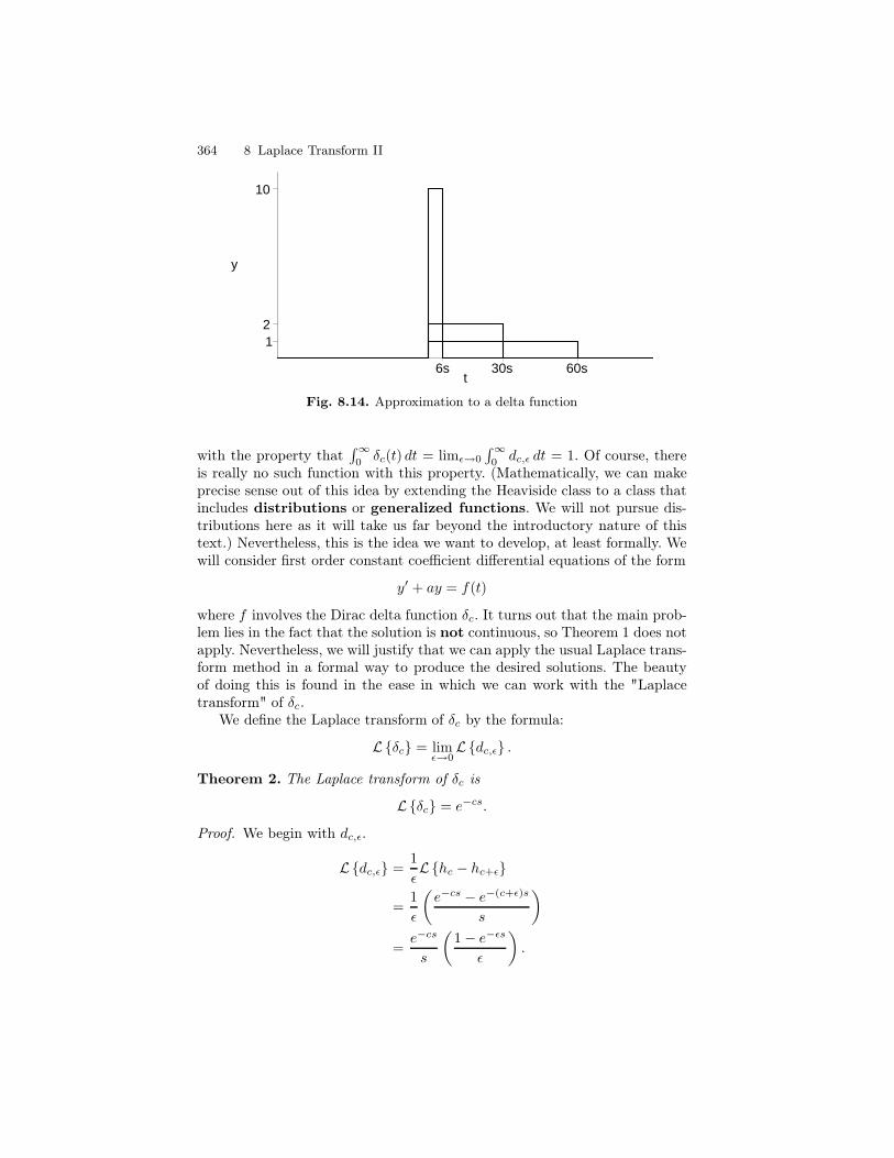
364 8 Laplace Transform II
1 2
10
y
6s 30s 60st
Fig. 8.14. Approximation to a delta function
with the property that∫∞0δc(t) dt = limε→0
∫∞0dc,ε dt = 1. Of course, there
is really no such function with this property. (Mathematically, we can makeprecise sense out of this idea by extending the Heaviside class to a class thatincludes distributions or generalized functions. We will not pursue dis-tributions here as it will take us far beyond the introductory nature of thistext.) Nevertheless, this is the idea we want to develop, at least formally. Wewill consider first order constant coefficient differential equations of the form
y′ + ay = f(t)
where f involves the Dirac delta function δc. It turns out that the main prob-lem lies in the fact that the solution is not continuous, so Theorem 1 does notapply. Nevertheless, we will justify that we can apply the usual Laplace trans-form method in a formal way to produce the desired solutions. The beautyof doing this is found in the ease in which we can work with the "Laplacetransform" of δc.
We define the Laplace transform of δc by the formula:
Lδc = limε→0Ldc,ε .
Theorem 2. The Laplace transform of δc is
Lδc = e−cs.
Proof. We begin with dc,ε.
Ldc,ε =1
εLhc − hc+ε
=1
ε
(
e−cs − e−(c+ε)s
s
)
=e−cs
s
(
1− e−εs
ε
)
.
8.5 The Dirac Delta Function 365
We now take limits as ε goes to 0 and use L’Hospitals rule to obtain:
Lδc = limε→0Ldc,ε =
e−cs
s
(
limε→0
1− e−εs
ε
)
=e−cs
s· s = e−cs.
ut
We remark that when c = 0 we have Lδ0 = 1. By Theorem 1 thereis no Heaviside function with this property. Thus, to reiterate, even thoughLδc is a function, δc is not. We will frequently write δ = δ0. Observe thatδc(t) = δ(t− c).
The mixing problem from Example 1 gives rise to a first order linear dif-ferential equation involving the Dirac delta function.
I Solution. Let y(t) be the amount of salt in the tank at time t. Theny(0) = 20 and y′ is the difference of the input rate and the output rate. Theonly input of salt occurs at t = 5. If the salt were input over a small interval,[5, 5+ ε) say, then 3
εχ[5,5+ε) would represent the input of 3 pounds of salt overa period of ε minutes. If we let ε go to zero then 3δ5 would represent the inputrate. The output rate is y(t)/10. We are thus led to the differential equation:
y′ +y
10= 3δ5, y(0) = 20.
J
The solution to this differential equation will fall out of the slightly moregeneral discussion we give below.
Differential Equations of the form y′ + ay = kδc
We will present progressively four methods for solving
y′ + ay = kδc, y(0) = y0. ?
The last method, the formal Laplace Transform Method, is the simplestmethod and is, in part, justified by the methods that precede it. The formalmethod will thereafter be used to solve equations of the form ? and will workfor all the problems introduced in this section. Keep in mind though that inpractice a careful analysis of the limiting processes involved must be done todetermine the validity of the formal Laplace Transform method.
Method 1. In our first approach we solve the equation
y′ + ay =k
εχ[c,c+ε), y(0) = y0
and call the solution yε. We let y(t) = limε→0 yε. Then y(t) is the solution toy′ + ay = kδc, y(0) = y0. Recall from Exercise ?? the solution to
366 8 Laplace Transform II
y′ + ay = Aχ[α, β), y(0) = y0,
is
y(t) = y0e−at +
A
a
0 if 0 ≤ t < α
1− e−a(t−α) if α ≤ t < β
e−a(t−β) − e−a(t−α) if β ≤ t <∞.
We let A = kε , α = c, and β = c+ ε to get
yε(t) = y0e−at +
k
aε
0 if 0 ≤ t < c
1− e−a(t−c) if c ≤ t < c+ ε
e−a(t−c−ε) − e−a(t−c) if c+ ε ≤ t <∞.
The computation of limε→0 yε is done on each interval separately. If 0 ≤ t ≤ cthen yε = y0e
−at is independent of ε and hence
limε→0
yε(t) = y0e−at 0 ≤ t ≤ c.
If c < t <∞ then for ε small enough, c+ ε < t and thus
yε(t) = y0e−at +
k
aε(e−a(t−c−ε) − e−a(t−c)) = y0e
−at +k
ae−a(t−c) e
aε − 1
ε.
Thereforelimε→0
yε(t) = y0e−at + ke−a(t−c) c < t <∞.
We thus obtain
y(t) =
y0e−at if 0 ≤ t ≤ c
y0e−at + ke−a(t−c) if c < t <∞.
In the mixing problem above the infusion of 3 pounds of salt after fiveminutes will instantaneously increase the amount of salt by 3; a jump dis-continuity at t = 5. This is seen in the solution y above. At t = c there is ajump discontinuity of jump k. Of course, the solution to the mixing problemis obtained by setting a = 1
10 , k = 3, c = 5, and y0 = 20:
y(t) =
20e−t10 if 0 ≤ t ≤ 5
20e−t10 + 3e−
t−510 if 5 < t <∞,
whose graph is given in Figure 8.15. We observe that y(5−) = 20e−1/2 ' 12.13and y(5+) = 20e−1/2 + 3 ' 15.13. Also notice that y(5+) is y(5−) plus thejump 3.
Method 2. Our second approach realizes that the mixing problem statedabove can be thought of as the differential equation, y′ + 1
10y = 0, defined ontwo separate intervals; (1) on the interval [0, 5) with initial value y(0) = 20
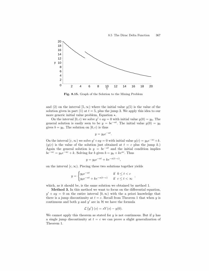
8.5 The Dirac Delta Function 367
0
2468
101214161820
y
2 4 6 8 10 12 14 16 18 20t
Fig. 8.15. Graph of the Solution to the Mixing Problem
and (2) on the interval [5,∞) where the initial value y(5) is the value of thesolution given in part (1) at t = 5, plus the jump 3. We apply this idea to ourmore generic initial value problem, Equation ?.
On the interval [0, c) we solve y′ +ay = 0 with initial value y(0) = y0. Thegeneral solution is easily seen to be y = be−at. The initial value y(0) = y0gives b = y0. The solution on [0, c) is thus
y = y0e−at.
On the interval [c,∞) we solve y′+ay = 0 with initial value y(c) = y0e−ac+k.
(y(c) is the value of the solution just obtained at t = c plus the jump k.)Again the general solution is y = be−at and the initial condition impliesbe−ac = y0e
−ac + k. Solving for b gives b = y0 + keac. Thus
y = y0e−at + ke−a(t−c),
on the interval [c,∞). Piecing these two solutions together yields
y =
y0e−at if 0 ≤ t < c
y0e−at + ke−a(t−c) if c ≤ t <∞ ,
which, as it should be, is the same solution we obtained by method 1.Method 3. In this method we want to focus on the differential equation,
y′ + ay = 0 on the entire interval [0,∞) with the a priori knowledge thatthere is a jump discontinuity at t = c. Recall from Theorem 1 that when y iscontinuous and both y and y′ are in H we have the formula
Ly′ (s) = sY (s)− y(0).
We cannot apply this theorem as stated for y is not continuous. But if y hasa single jump discontinuity at t = c we can prove a slight generalization ofTheorem 1.
368 8 Laplace Transform II
Theorem 3. Suppose y and y′ are in H and y is continuous except for onejump discontinuity at t = c with jump k. Then
Ly′ (s) = sY (s)− y(0)− ke−cs.
Proof. Let N > c. Then integration by parts gives
∫ N
0
e−sty′(t) dt =
∫ c
0
e−sty(t) dt+
∫ N
c
e−sty(t) dt
= e−sty(t)|c0 + s
∫ c
0
e−sty(t) dt+ e−sty(t)|Nc + s
∫ N
c
e−sty(t) dt
= s
∫ N
0
e−sty(t) dt+ e−sNy(N)− y(0)− e−sc(y(c+)− y(c−).
We take the limit as N goes to infinity and obtain:
Ly′ = sLy − y(0)− ke−sc.
ut
We apply this theorem to the initial value problem
y′ + ay = 0, y(0) = y0
with the knowledge that the solution y has a jump discontinuity at t = c withjump k. Apply the Laplace transform to to the differential equation to obtain:
sY (s)− y(0)− ke−ac + aY (s) = 0.
Solving for Y gives
Y (s) =y0s+ a
+ ke−as
s+ a.
Applying the inverse Laplace transform gives the solution
y(t) = y0e−at + ke−a(t−c)hc(t)
=
y0e−at if 0 ≤ t < c
y0e−at + ke−a(t−c) if c ≤ t <∞.
Method 4: The Formal Laplace Transform Method. We now returnto the differential equation
y′ + ay = kδc, y(0) = y0
and apply the Laplace transform method directly. That we can do this is partlyjustified by method 3 above. From Theorem 2 the Laplace transform of kδc iske−sc. This is precisely the term found in Theorem 3 where the assumption ofa single jump discontinuity is assumed. Thus the presence of kδc automatically
8.6 Impulse Functions 369
encodes the jump discontinuity in the solution. Therefore we can (formally)proceed without any advance knowledge of jump discontinuities. The Laplacetransform of
y′ + ay = kδc, y(0) = y0
givessY (s)− y(0) + kY (s) = ke−sc
and one proceeds as at the end of method 3 to get
y(t) =
y0e−at if 0 ≤ t < c
y0e−at + ke−a(t−c) if c ≤ t <∞.
8.6 Impulse Functions
An impulsive force is a force with high magnitude introduced over a shortperiod of time. For example, a bat hitting a ball or a spike in electricityon an electric circuit both involve impulsive forces and are best representedby the Dirac delta function. In this section we will consider the effect of theintroduction of impulsive forces into such systems and how they lead to secondorder differential equations of the form
my′′ + µy′ + ky = Kδc(t).
As we will soon see the effect of an impulsive force introduces a discontinuitynot in y but its derivative y′.
If F (t) represents a force which is 0 outside a time interval [a, b] then∫∞0 F (t) dt =
∫ b
a F (t) dt represents the total impulse of the force F (t) overthat interval. A unit impulse means that this integral is 1. If F is given bythe acceleration of a constant mass then F (t) = ma(t), where m is the massand a(t) is the acceleration. The total impulse
∫ b
a
F (t) dt =
∫ b
a
ma(t) dt = mv(b)−mv(a)
represents the change of momentum. (Momentum is the product of mass andvelocity). Now imagine this force is introduced over a very short period oftime, or even instantaneously. As in the previous section, we could model theforce by dc,ε = 1
εχ[c,c+ε) and one would naturally be lead to the Dirac deltafunction to represent the instantaneous change of momentum. Since momen-tum is proportional to velocity we see that such impacts lead to discontinuitiesin the derivative y′.
370 8 Laplace Transform II
Example 1. (see Chapter ?? for a discussion of spring-mass-dashpot sys-tems) A spring is stretched 49 cm when a 1 kg mass is attached. The body ispulled to 10 cm below its spring-body equilibrium and released. We assumethe system is frictionless. After 3 sec the mass is suddenly struck by a hammerin a downward direction with total impulse of 4 kg·m/sec. Find the motion ofthe mass.
I Solution. We will work in units of kg, m, and sec. Thus the spring con-stant k is given by 1(9.8) = k 49
100 , so that k = 20. The initial conditions aregiven by y(0) = .10 and y′(0) = 0, and since the system is frictionless therewritten initial value problem is
y′′ + 20y = 4δ3, y(0) = .10, y′(0) = 0.
J
We will return to the solution of this problem after we discuss the moregeneral second order case.
Differential Equations of the form
y′′ + ay′ + by = Kδc
Our goal is to solve
y′′ + ay′ + by = Kδc, y(0) = y0, y′(0) = y1 ?
using the formal Laplace transform method that we discussed in Method 4 ofSection 8.5.
As we discussed above the effect of Kδc is to introduce a single jumpdiscontinuity in y′ at t = c with jump K. Therefore the solution to (?) isequivalent to solving
y′′ + ay′ + by = 0
with the advanced knowledge that y′ has a jump discontinuity at t = c. If weapply Theorem 3 to y′ we obtain
Ly′′ = sLy′ − y′(0)−Ke−sc
= s2Y (s)− sy(0)− y′(0)−Ke−sc
Therefore, the Laplace transform of y′′ + ay′ + by = 0 leads to
(s2 + as+ b)Y (s)− sy(0)− y′(0)−Ke−sc = 0.
On the other hand, if we (formally) proceed with the Laplace transform ofEquation (?) without foreknowledge of discontinuities we obtain the equivalentequation
(s2 + as+ b)Y (s)− sy(0)− y′(0) = Ke−sc.
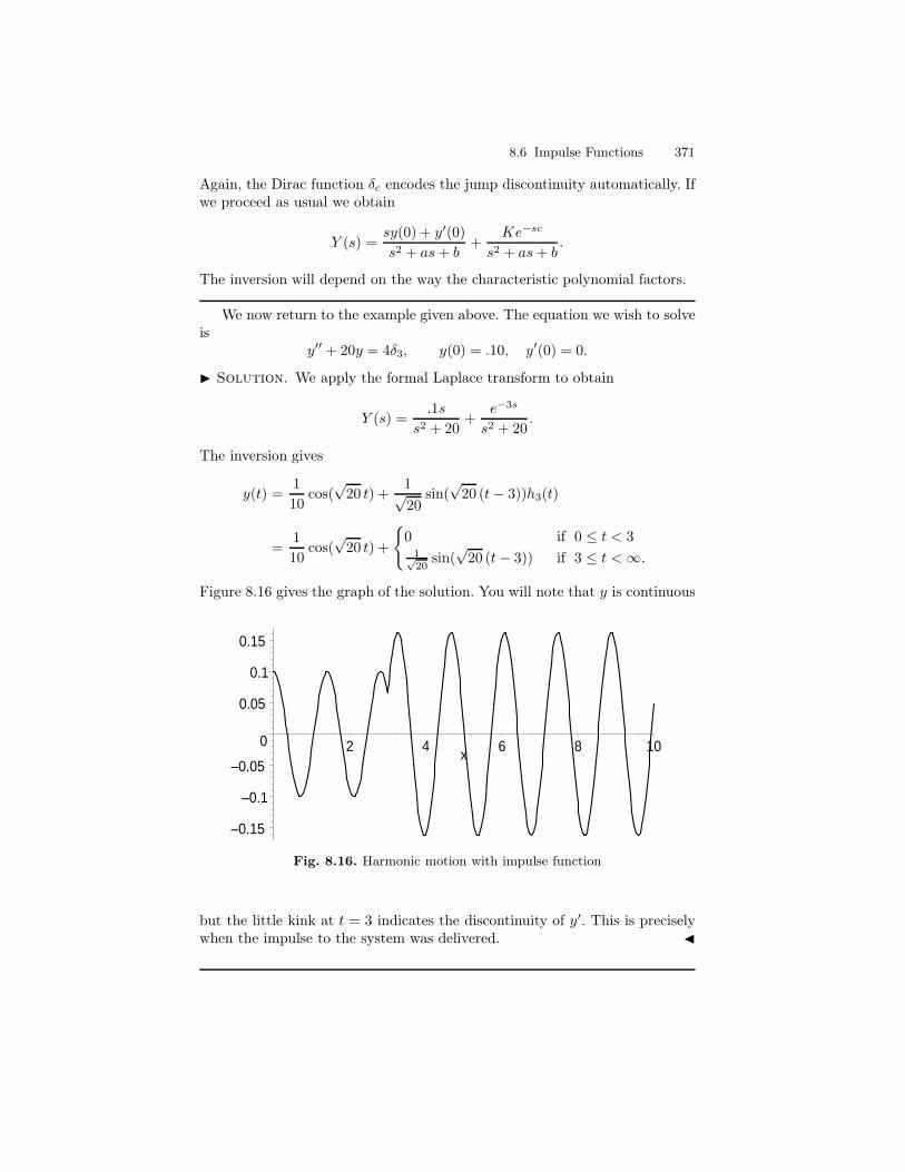
8.6 Impulse Functions 371
Again, the Dirac function δc encodes the jump discontinuity automatically. Ifwe proceed as usual we obtain
Y (s) =sy(0) + y′(0)
s2 + as+ b+
Ke−sc
s2 + as+ b.
The inversion will depend on the way the characteristic polynomial factors.
We now return to the example given above. The equation we wish to solveis
y′′ + 20y = 4δ3, y(0) = .10, y′(0) = 0.
I Solution. We apply the formal Laplace transform to obtain
Y (s) =.1s
s2 + 20+
e−3s
s2 + 20.
The inversion gives
y(t) =1
10cos(√
20 t) +1√20
sin(√
20 (t− 3))h3(t)
=1
10cos(√
20 t) +
0 if 0 ≤ t < 31√20
sin(√
20 (t− 3)) if 3 ≤ t <∞.
Figure 8.16 gives the graph of the solution. You will note that y is continuous
–0.15
–0.1
–0.05
0
0.05
0.1
0.15
2 4 6 8 10x
Fig. 8.16. Harmonic motion with impulse function
but the little kink at t = 3 indicates the discontinuity of y′. This is preciselywhen the impulse to the system was delivered. J
372 8 Laplace Transform II
Exercises
Solve each of the following initial value problems.
1. y′ + 2y = δ1(t), y(0) = 02. y′ + 2y = δ1(t), y(0) = 13. y′ + 2y = δ1(t) − δ3(t), y(0) = 04. y′′ + 4y = δπ(t), y(0) = 0, y′(0) = 15. y′′ + 4y = δπ(t) − δ2π(t), y(0) = 0, y′(0) = 06. y′′ + 4y = δπ(t) − δ2π(t), y(0) = 1, y′(0) = 07. y′′ + 4y′ + 4y = 3δ1(t), y(0) = 0, y′(0) = 08. y′′ + 4y′ + 4y = 3δ1(t), y(0) = −1, y′(0) = 39. y′′ + 4y′ + 5y = 3δ1(t), y(0) = 0, y′(0) = 0
10. y′′ + 4y′ + 5y = 3δ1(t), y(0) = −1, y′(0) = 311. y′′ + 4y′ + 20y = δπ(t) − δ2π(t), y(0) = 1, y′(0) = 012. y′′ − 4y′ − 5y = 2e−t + δ3(t), y(0) = 0, y′(0) = 0
8.7 Periodic Functions
In modelling mechanical and other systems it frequently happens that theforcing function repeats over time. Periodic functions best model such repeti-tion.
A function f defined on [0,∞) is said to be periodic if there is a positivenumber p such that f(t+ p) = f(t) for all t in the domain of f . We say p is aperiod of f . If p > 0 is a period of f and there is no smaller period then wesay p is the fundamental period of f although we will usually just say theperiod. The interval [0, p) is called the fundamental interval. If there is nosuch smallest positive p for a periodic function then the period is defined tobe 0. The constant function f(t) = 1 is an example of a periodic function withperiod 0. The sine function is periodic with period 2π: sin(t + 2π) = sin(t).Knowing the sine on the interval [0, 2π) implies knowledge of the functioneverywhere. Similarly, if we know f is periodic with period p > 0 and weknow the function on the fundamental interval then we know the functioneverywhere. Figure 8.17 illustrates this point.
The Sawtooth Function
A particularly useful periodic function is the sawtooth function. With it wecan express other periodic functions simply by composition. Let p > 0. Thesaw tooth function is given by
< t >p=
t if 0 ≤ t < p
t− p if p ≤ t < 2p
t− 2p if 2p ≤ t < 3p...
.
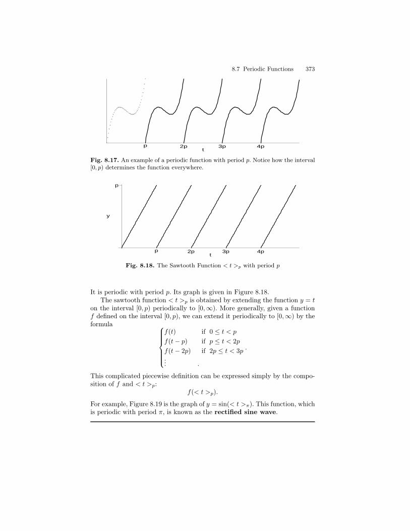
8.7 Periodic Functions 373
p 2p 3p 4pt
Fig. 8.17. An example of a periodic function with period p. Notice how the interval[0, p) determines the function everywhere.
p
y
p 2p 3p 4pt
Fig. 8.18. The Sawtooth Function < t >p with period p
It is periodic with period p. Its graph is given in Figure 8.18.The sawtooth function < t >p is obtained by extending the function y = t
on the interval [0, p) periodically to [0,∞). More generally, given a functionf defined on the interval [0, p), we can extend it periodically to [0,∞) by theformula
f(t) if 0 ≤ t < p
f(t− p) if p ≤ t < 2p
f(t− 2p) if 2p ≤ t < 3p... .
.
This complicated piecewise definition can be expressed simply by the compo-sition of f and < t >p:
f(< t >p).
For example, Figure 8.19 is the graph of y = sin(< t >π). This function, whichis periodic with period π, is known as the rectified sine wave.
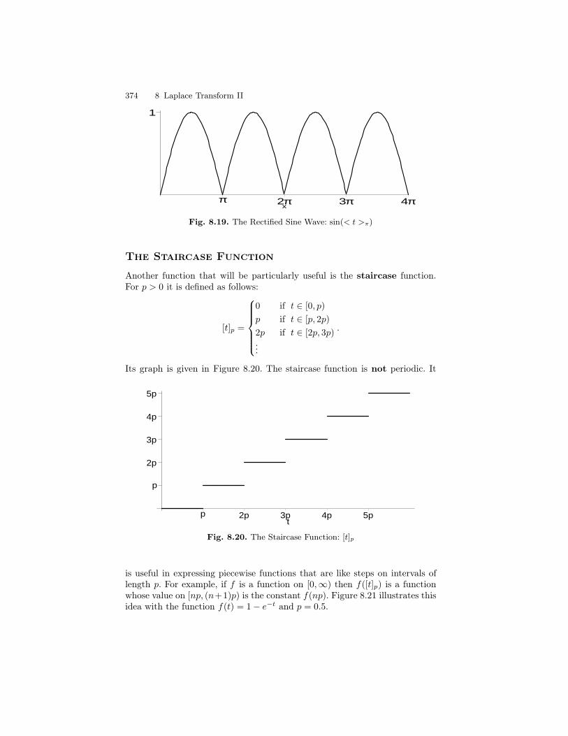
374 8 Laplace Transform II
1
π 2π 3π 4πx
Fig. 8.19. The Rectified Sine Wave: sin(< t >π)
The Staircase Function
Another function that will be particularly useful is the staircase function.For p > 0 it is defined as follows:
[t]p =
0 if t ∈ [0, p)
p if t ∈ [p, 2p)
2p if t ∈ [2p, 3p)...
.
Its graph is given in Figure 8.20. The staircase function is not periodic. It
p
2p
3p
4p
5p
p 2p 3p 4p 5pt
Fig. 8.20. The Staircase Function: [t]p
is useful in expressing piecewise functions that are like steps on intervals oflength p. For example, if f is a function on [0,∞) then f([t]p) is a functionwhose value on [np, (n+1)p) is the constant f(np). Figure 8.21 illustrates thisidea with the function f(t) = 1− e−t and p = 0.5.
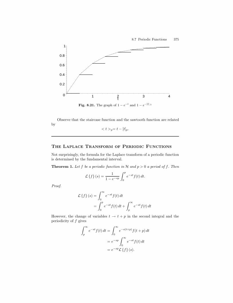
8.7 Periodic Functions 375
0
0.2
0.4
0.6
0.8
1
1 2 3 4t
Fig. 8.21. The graph of 1 − e−t and 1 − e−[t].5
Observe that the staircase function and the sawtooth function are relatedby
< t >p= t− [t]p.
The Laplace Transform of Periodic Functions
Not surprisingly, the formula for the Laplace transform of a periodic functionis determined by the fundamental interval.
Theorem 1. Let f be a periodic function in H and p > 0 a period of f . Then
Lf (s) =1
1− e−sp
∫ p
0
e−stf(t) dt.
Proof.
Lf (s) =
∫ ∞
0
e−stf(t) dt
=
∫ p
0
e−stf(t) dt+
∫ ∞
p
e−stf(t) dt
However, the change of variables t → t + p in the second integral and theperiodicity of f gives
∫ ∞
p
e−stf(t) dt =
∫ ∞
0
e−s(t+p)f(t+ p) dt
= e−sp
∫ ∞
0
e−stf(t) dt
= e−spLf (s).
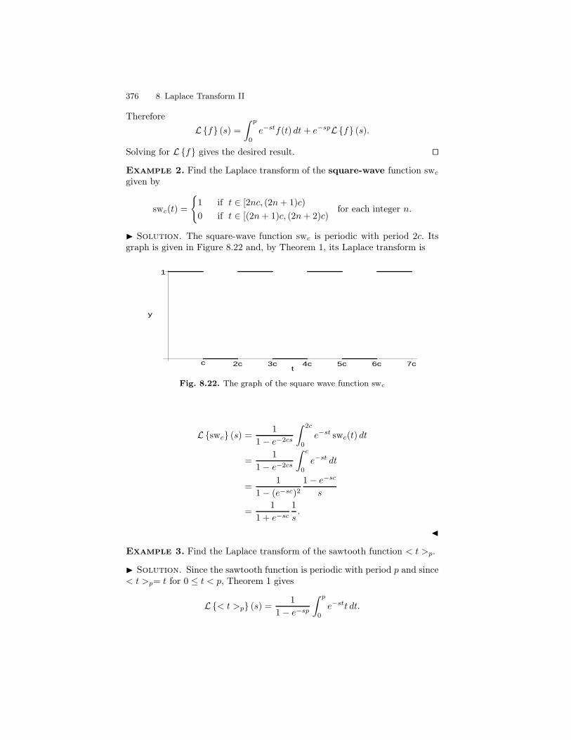
376 8 Laplace Transform II
Therefore
Lf (s) =
∫ p
0
e−stf(t) dt+ e−spLf (s).
Solving for Lf gives the desired result. ut
Example 2. Find the Laplace transform of the square-wave function swc
given by
swc(t) =
1 if t ∈ [2nc, (2n+ 1)c)
0 if t ∈ [(2n+ 1)c, (2n+ 2)c)for each integer n.
I Solution. The square-wave function swc is periodic with period 2c. Itsgraph is given in Figure 8.22 and, by Theorem 1, its Laplace transform is
1
y
c 2c 3c 4c 5c 6c 7ct
Fig. 8.22. The graph of the square wave function swc
Lswc (s) =1
1− e−2cs
∫ 2c
0
e−st swc(t) dt
=1
1− e−2cs
∫ c
0
e−st dt
=1
1− (e−sc)21− e−sc
s
=1
1 + e−sc
1
s.
J
Example 3. Find the Laplace transform of the sawtooth function < t >p.
I Solution. Since the sawtooth function is periodic with period p and since< t >p= t for 0 ≤ t < p, Theorem 1 gives
L< t >p (s) =1
1− e−sp
∫ p
0
e−stt dt.
8.7 Periodic Functions 377
Integration by parts gives∫ p
0
e−stt dt =te−st
−s |p0−
1
−s
∫ p
0
e−st dt = −pe−sp
s− 1
s2e−st|p0 = −pe
−sp
s−e
−sp − 1
s2.
With a little algebra we obtain
L< t >p (s) =1
s2(1− spe−sp
1− e−sp).
J
As mentioned above it frequently happens that we build periodic functionsby restricting a given function f to the interval [0, p) and then extending it tobe periodic with period p: f(< t >p). Suppose now that f ∈ H. We can thenexpress the Laplace transform of f(< t >p) in terms of the Laplace transformof f . The following corollary expresses this relationship and simplifies unnec-essary calculations like the integration by parts that we did in the previousexample.
Corollary 4. Let p > 0 Suppose f ∈ H. Then
Lf(< t >p) (s) =1
1− e−spLf − fhp .
Proof. The function f−fhp = f(1−hp) is the same as f on the interval [0, p)and 0 on the interval [p,∞).. Therefore
∫ p
0
e−stf(t) dt =
∫ ∞
0
e−st(f(t)− f(t)hp(t)) dt = Lf − fhp .
The result now follows from Theorem 1. ut
Let’s return to the sawtooth function in Example 3 and see how Corollary4 simplifies the calculation of its Laplace transform.
L< t >p (s) =1
1− e−spLt− thp
=1
1− e−sp
(
1
s2− e−spLt+ p
)
=1
1− e−sp
(
1
s2− e−sp 1 + sp
s2
)
=1
s2
(
1− spe−sp
1− e−sp
)
.
The last line requires a few algebraic steps.
Example 5. Find the Laplace transform of the rectified sine wave sin(<t >π). See Figure 8.19.
378 8 Laplace Transform II
I Solution. Corollary 4 gives
Lsin(< t >π) =1
1− e−πsLsin t− sin t hπ(t)
=1
1− e−πs
(
1
s2 + 1− e−πsLsin(t+ π)
)
=1
1− e−πs
(
1 + e−πs
s2 + 1
)
,
where we use the fact that sin(t+ π) = − sin(t). J
The inverse Laplace transform
The inverse Laplace transform of functions of the form
1
1− e−spF (s)
is not always a straightforward matter to find unless, of course, F (s) is of theform Lf − fhp so that Corollary 4 can be used. Usually though this is notthe case. Let r be a fixed real or complex number. Recall that the geometricseries ∞
∑
n=0
rn = 1 + r + r2 + r3 + · · ·
converges to 11−r when |r| < 1. Since e−sp < 1 for s > 0 we can write
1
1− e−sp=
∞∑
n=0
e−snp
and therefore1
1− e−spF (s) =
∞∑
n=0
e−snpF (s).
If f = L−1 F then a termwise computation gives
L−1
1
1− e−spF (s)
=
∞∑
n=0
L−1
e−snpF (s)
=
∞∑
n=0
f(t− np)hnp(t).
On an interval of the form [Np, (N+1)p) the function hnp is 1 for n = 0, . . . , Nand 0 otherwise. We thus obtain
L−1
1
1− e−spF (s)
=∞∑
N=0
(
N∑
n=0
f(t− np))
χ[Np,(N+1)p).
8.7 Periodic Functions 379
A similar argument gives
L−1
1
1 + e−spF (s)
=
∞∑
N=0
(
N∑
n=0
(−1)nf(t− np))
χ[Np,(N+1)p).
For reference we record these results in the following theorem:
Theorem 6. Let p > 0 and suppose Lf(t) = F (s). Then
1. L−1
11−e−spF (s)
=∑∞
N=0
(
∑Nn=0 f(t− np)
)
χ[Np,(N+1)p).
2. L−1
11+e−spF (s)
=∑∞
N=0
(
∑Nn=0(−1)nf(t− np)
)
χ[Np,(N+1)p).
Example 7. Find the inverse Laplace transform of
1
(1 − e−2s)s.
I Solution. If f(t) = 1 then F (s) = 1s is its Laplace transform. We thus
have
L−1
1
(1− e−2s)s
=∞∑
N=0
(
N∑
n=0
f(t− 2n)
)
χ[2N,2(N+1))
=
∞∑
N=0
(N + 1)χ[2N,2(N+1))
= 1 +1
2
∞∑
N=0
2Nχ[2N,2(N+1))
= 1 +1
2[t]2.
J
Mixing Problems with Periodic Input
We now turn our attention to two examples. Both are mixing problems withperiodic input functions.
Example 8. Suppose a tank contains 10 gallons of pure water. Two inputsources alternately flow into the tank for 1 minute intervals. The first inputsource is a brine solution with concentration 1 pound salt per gallon and flows(when on) at a rate of 5 gallons per minute. The second input source is purewater and flows (when on) at a rate of 5 gallons per minute. The tank hasa drain with a constant outflow of 5 gallons per minute. Let y(t) denote thetotal amount of salt at time t. Find y(t) and for large values of t determinehow y(t) fluctuates.
380 8 Laplace Transform II
I Solution. The input rate of salt is given piecewise by the formula
5 if 2n ≤ t < 2n+ 1)
0 if 2n+ 1 ≤ t < 2n+ 2= 5 sw1(t).
The output rate is given byy(t)
10· 5.
This leads to the first order differential equation
y′ +1
2y = 5 sw1(t) y(0) = 0.
A calculation using Example 2 gives that the Laplace transform is
Y (s) = 51
1 + e−s
1
s(s+ 12 ),
and a partial fraction decomposition gives
Y (s) = 101
1 + e−s
1
s− 10
1
1 + e−s
1
s+ 12
.
Now apply the inverse Laplace transform. By Theorem 6 the inverse Laplacetransform of the first expression is
10
∞∑
N=0
N∑
n=0
(−1)nχ[N,N+1) = 10
∞∑
N=0
χ[2N,2N+1) = 10 sw1(t).
By Theorem 6 the inverse Laplace transform of the second expression is
10∞∑
N=0
N∑
n=0
(−1)ne−12 (t−n)χ[N,N+1) = 10e−
12 t
∞∑
N=0
N∑
n=0
(−e 12 )nχ[N,N+1)
= 10e−12 t
∞∑
N=0
1− (−e 12 )N+1
1 + e12
χ[N,N+1)
=10e−
12 t
1 + e12
1 + eN+1
2 if t ∈ [N,N + 1) (N even)
1− eN+12 if t ∈ [N,N + 1) (N odd)
.
Finally, we put these two expression together to get our solution
y(t) = 10 sw1(t)−10e−
12 t
1 + e12
1 + eN+1
2 if t ∈ [N,N + 1) (N even)
1− eN+12 if t ∈ [N,N + 1) (N odd)
(1)
=
10− 10 e−12
t+e−t+N+1
2
1+e12
if t ∈ [N,N + 1) (N even)
−10 e−12
t−e−t+N+1
2
1+e12
if t ∈ [N,N + 1) (N odd)
.
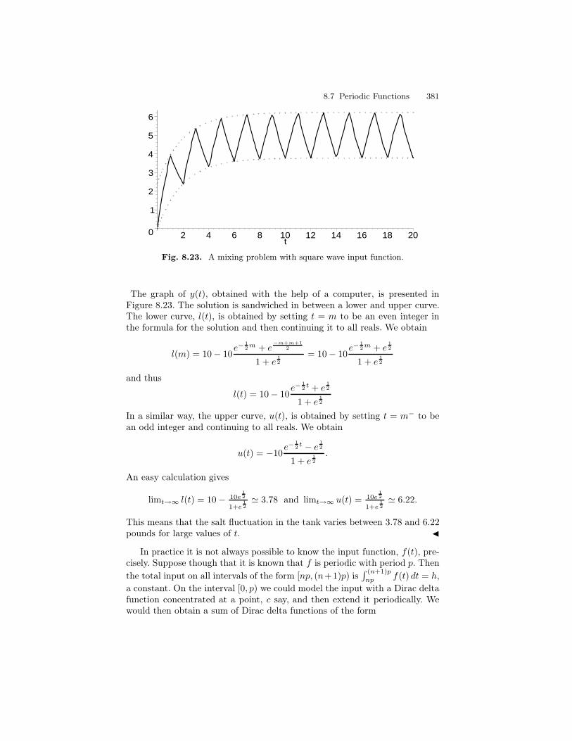
8.7 Periodic Functions 381
0
1
2
3
4
5
6
2 4 6 8 10 12 14 16 18 20t
Fig. 8.23. A mixing problem with square wave input function.
The graph of y(t), obtained with the help of a computer, is presented inFigure 8.23. The solution is sandwiched in between a lower and upper curve.The lower curve, l(t), is obtained by setting t = m to be an even integer inthe formula for the solution and then continuing it to all reals. We obtain
l(m) = 10− 10e−
12m + e
−m+m+12
1 + e12
= 10− 10e−
12m + e
12
1 + e12
and thus
l(t) = 10− 10e−
12 t + e
12
1 + e12
In a similar way, the upper curve, u(t), is obtained by setting t = m− to bean odd integer and continuing to all reals. We obtain
u(t) = −10e−
12 t − e 1
2
1 + e12
.
An easy calculation gives
limt→∞ l(t) = 10− 10e12
1+e12' 3.78 and limt→∞ u(t) = 10e
12
1+e12' 6.22.
This means that the salt fluctuation in the tank varies between 3.78 and 6.22pounds for large values of t. J
In practice it is not always possible to know the input function, f(t), pre-cisely. Suppose though that it is known that f is periodic with period p. Thenthe total input on all intervals of the form [np, (n+1)p) is
∫ (n+1)p
np f(t) dt = h,a constant. On the interval [0, p) we could model the input with a Dirac deltafunction concentrated at a point, c say, and then extend it periodically. Wewould then obtain a sum of Dirac delta functions of the form
382 8 Laplace Transform II
a(t) = h(δc + δc+p + δc+2p + · · · )
that may adequately represent the input for the system we are trying to model.Additional information may justify distributing the total input over two ormore points in the interval and extend periodically. Whatever choices are madethe solution will need to be analyzed in the light of empirical data known aboutthe system. Consider the example above. Suppose that it is known that theinput is periodic with period 2 and total input 5 on the fundamental interval.Suppose additionally that you are told that the distribution of the input ofsalt is on the first half of each interval. We might be led to try to model theinput on [0, 2) by 5
2δ0 + 52δ1 and then extend periodically to obtain
a(t) =5
2
∞∑
n=0
δn.
Of course, the solution modelled by the input function a(t) will differ from theactual solution. What is true though is that both exhibit similar long termbehavior. This can be observed in the following example.
Example 9. Suppose a tank contains 10 gallons of pure water. Pure waterflows into the tank at a rate of 5 gallons per minute. The tank has a drainwith a constant outflow of 5 gallons per minute. Suppose 5
2 pounds of salt isput in the tank each minute whereupon it instantly and uniformly dissolves.Assume the level of fluid in the tank is always 10 gallons. Let y(t) denote thetotal amount of salt at time t. Find y(t) and for large values of t determinehow y(t) fluctuates.
I Solution. As discussed above the input function is 52
∑∞n=1 δn and there-
fore the differential equation that models this system is
y′ +1
2y =
5
2
∞∑
n=1
δn, y(0) = 0.
The Laplace transform leads to
Y (s) =5
2
∞∑
n=0
e−sn 1
s+ 12
,
and inverting the Laplace transform gives
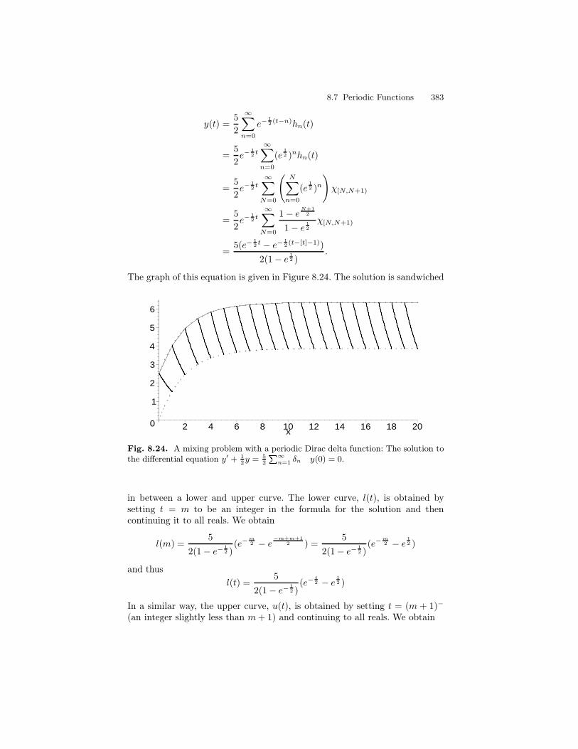
8.7 Periodic Functions 383
y(t) =5
2
∞∑
n=0
e−12 (t−n)hn(t)
=5
2e−
12 t
∞∑
n=0
(e12 )nhn(t)
=5
2e−
12 t
∞∑
N=0
(
N∑
n=0
(e12 )n
)
χ[N,N+1)
=5
2e−
12 t
∞∑
N=0
1− eN+12
1− e 12
χ[N,N+1)
=5(e−
12 t − e− 1
2 (t−[t]−1))
2(1− e 12 )
.
The graph of this equation is given in Figure 8.24. The solution is sandwiched
0
1
2
3
4
5
6
2 4 6 8 10 12 14 16 18 20x
Fig. 8.24. A mixing problem with a periodic Dirac delta function: The solution tothe differential equation y′ + 1
2y = 5
2
∞n=1 δn y(0) = 0.
in between a lower and upper curve. The lower curve, l(t), is obtained bysetting t = m to be an integer in the formula for the solution and thencontinuing it to all reals. We obtain
l(m) =5
2(1− e− 12 )
(e−m2 − e−m+m+1
2 ) =5
2(1− e− 12 )
(e−m2 − e 1
2 )
and thus
l(t) =5
2(1− e− 12 )
(e−t2 − e 1
2 )
In a similar way, the upper curve, u(t), is obtained by setting t = (m + 1)−
(an integer slightly less than m+ 1) and continuing to all reals. We obtain
384 8 Laplace Transform II
u(t) =5
2(1− e− 12 )
(e−t2 − 1)
An easy calculation gives
limt→∞ l(t) = −5e12
2(1−e12 )' 3.85 and limt→∞ u(t) = −5
2(1−e12 )' 6.35.
This means that the salt fluctuation in the tank varies between 3.85 and 6.35pounds for large values of t. J
A comparison of the solutions in these examples reveals similar long termbehavior in the fluctuation of the salt content in the tank. Remember thoughthat each problem that is modelled must be weighed against hard empiricaldata to determine if the model is appropriate or not. Also, we could havemodelled the instantaneous input by assuming the input was concentrated ata single point, rather than two points. The results are not as favorable. Theseother possibilities are explored in the exercises.
8.8 Undamped Motion with Periodic Input
In Section ?? we discussed various kinds of harmonic motion that can resultfrom solutions to the differential equation
ay′′ + by′ + cy = f(t).
Undamped motion led to the differential equation
ay′′ + cy = f(t). (1)
In particular, we explored the case where f(t) = F0 cosωt and were led to thesolution
y(t) =
F0
a(β2 − ω2)(cosωt− cosβt) if β 6= ω
F0
2aωt sinωt if β = ω,
(2)
where β =√
ca . The case where β 6= ω gave rise to the notion of beats, while
the case β = ω gave us resonance. Since cosωt is periodic the system that ledto Equation 1 is an example of undamped motion with periodic input.In this section we will explore this phenomenon with two further examples: asquare wave periodic function, swc and a periodic impulse function,
∑∞n=0 δnc.
Both examples are algebraically tedious, so you will be asked to fill in some ofthe algebraic details in the exercises. To simplify the notation we will rewriteEquation (1) as
y′′ + β2y = g(t)
and assume y(0) = y′(0) = 0.
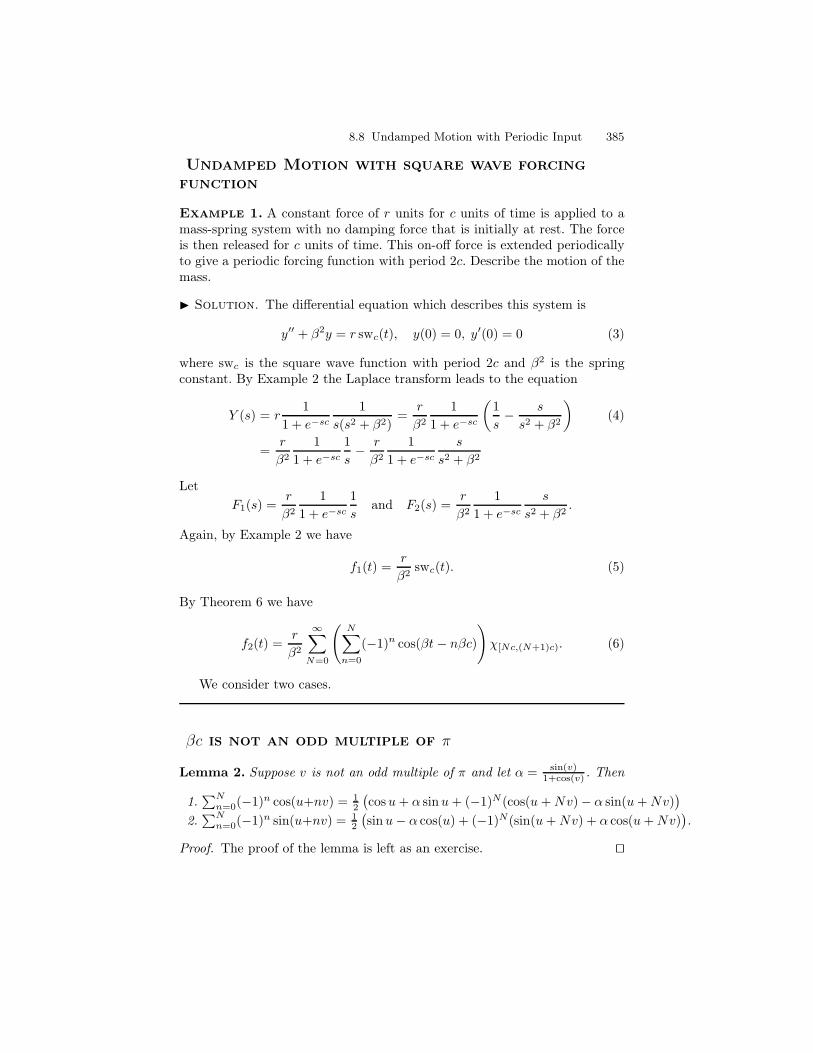
8.8 Undamped Motion with Periodic Input 385
Undamped Motion with square wave forcing
function
Example 1. A constant force of r units for c units of time is applied to amass-spring system with no damping force that is initially at rest. The forceis then released for c units of time. This on-off force is extended periodicallyto give a periodic forcing function with period 2c. Describe the motion of themass.
I Solution. The differential equation which describes this system is
y′′ + β2y = r swc(t), y(0) = 0, y′(0) = 0 (3)
where swc is the square wave function with period 2c and β2 is the springconstant. By Example 2 the Laplace transform leads to the equation
Y (s) = r1
1 + e−sc
1
s(s2 + β2)=
r
β2
1
1 + e−sc
(
1
s− s
s2 + β2
)
(4)
=r
β2
1
1 + e−sc
1
s− r
β2
1
1 + e−sc
s
s2 + β2
Let
F1(s) =r
β2
1
1 + e−sc
1
sand F2(s) =
r
β2
1
1 + e−sc
s
s2 + β2.
Again, by Example 2 we have
f1(t) =r
β2swc(t). (5)
By Theorem 6 we have
f2(t) =r
β2
∞∑
N=0
(
N∑
n=0
(−1)n cos(βt − nβc))
χ[Nc,(N+1)c). (6)
We consider two cases.
βc is not an odd multiple of π
Lemma 2. Suppose v is not an odd multiple of π and let α = sin(v)1+cos(v) . Then
1.∑N
n=0(−1)n cos(u+nv) = 12
(
cosu+ α sinu+ (−1)N (cos(u +Nv)− α sin(u+Nv))
2.∑N
n=0(−1)n sin(u+nv) = 12
(
sinu− α cos(u) + (−1)N(sin(u+Nv) + α cos(u+Nv))
.
Proof. The proof of the lemma is left as an exercise. ut
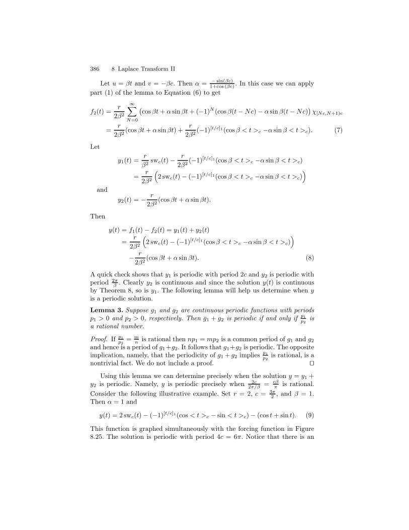
386 8 Laplace Transform II
Let u = βt and v = −βc. Then α = − sin(βc)1+cos (βc) . In this case we can apply
part (1) of the lemma to Equation (6) to get
f2(t) =r
2β2
∞∑
N=0
(
cosβt+ α sinβt+ (−1)N (cosβ(t−Nc)− α sinβ(t−Nc))
χ[Nc,N+1)c
=r
2β2(cosβt+ α sinβt) +
r
2β2(−1)[t/c]1(cosβ < t >c −α sinβ < t >c). (7)
Let
y1(t) =r
β2swc(t)−
r
2β2(−1)[t/c]1(cosβ < t >c −α sinβ < t >c)
=r
2β2
(
2 swc(t)− (−1)[t/c]1(cosβ < t >c −α sinβ < t >c))
and
y2(t) = − r
2β2(cosβt+ α sinβt).
Then
y(t) = f1(t)− f2(t) = y1(t) + y2(t)
=r
2β2
(
2 swc(t)− (−1)[t/c]1(cosβ < t >c −α sinβ < t >c))
− r
2β2(cos βt+ α sinβt). (8)
A quick check shows that y1 is periodic with period 2c and y2 is periodic withperiod 2π
β . Clearly y2 is continuous and since the solution y(t) is continuousby Theorem 8, so is y1. The following lemma will help us determine when yis a periodic solution.
Lemma 3. Suppose g1 and g2 are continuous periodic functions with periodsp1 > 0 and p2 > 0, respectively. Then g1 + g2 is periodic if and only if p1
p2is
a rational number.
Proof. If p1
p2= m
n is rational then np1 = mp2 is a common period of g1 and g2and hence is a period of g1+g2. It follows that g1+g2 is periodic. The oppositeimplication, namely, that the periodicity of g1 + g2 implies p1
p2is rational, is a
nontrivial fact. We do not include a proof. utUsing this lemma we can determine precisely when the solution y = y1 +
y2 is periodic. Namely, y is periodic precisely when 2c2π/β = cβ
π is rational.
Consider the following illustrative example. Set r = 2, c = 3π2 , and β = 1.
Then α = 1 and
y(t) = 2 swc(t)− (−1)[t/c]1(cos < t >c − sin < t >c)− (cos t+ sin t). (9)
This function is graphed simultaneously with the forcing function in Figure8.25. The solution is periodic with period 4c = 6π. Notice that there is an
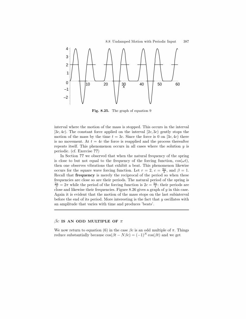
8.8 Undamped Motion with Periodic Input 387
–2
–1
0
1
2
3
4
10 20 30 40 50 60x
Fig. 8.25. The graph of equation 9
interval where the motion of the mass is stopped. This occurs in the interval[3c, 4c). The constant force applied on the interval [2c, 3c) gently stops themotion of the mass by the time t = 3c. Since the force is 0 on [3c, 4c) thereis no movement. At t = 4c the force is reapplied and the process thereafterrepeats itself. This phenomenon occurs in all cases where the solution y isperiodic. (cf. Exercise ??)
In Section ?? we observed that when the natural frequency of the springis close to but not equal to the frequency of the forcing function, cos(ωt),then one observes vibrations that exhibit a beat. This phenomenon likewiseoccurs for the square wave forcing function. Let r = 2, c = 9π
8 , and β = 1.Recall that frequency is merely the reciprocal of the period so when thesefrequencies are close so are their periods. The natural period of the spring is2πβ = 2π while the period of the forcing function is 2c = 9π
4 : their periods areclose and likewise their frequencies. Figure 8.26 gives a graph of y in this case.Again it is evident that the motion of the mass stops on the last subintervalbefore the end of its period. More interesting is the fact that y oscillates withan amplitude that varies with time and produces ’beats’.
βc is an odd multiple of π
We now return to equation (6) in the case βc is an odd multiple of π. Thingsreduce substantially because cos(βt−Nβc) = (−1)N cos(βt) and we get
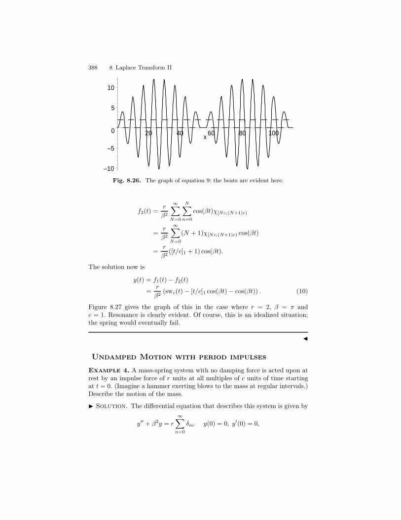
388 8 Laplace Transform II
–10
–5
0
5
10
20 40 60 80 100x
Fig. 8.26. The graph of equation 9: the beats are evident here.
f2(t) =r
β2
∞∑
N=0
N∑
n=0
cos(βt)χ[Nc,(N+1)c)
=r
β2
∞∑
N=0
(N + 1)χ[Nc,(N+1)c) cos(βt)
=r
β2([t/c]1 + 1) cos(βt).
The solution now is
y(t) = f1(t)− f2(t)=
r
β2(swc(t)− [t/c]1 cos(βt)− cos(βt)) . (10)
Figure 8.27 gives the graph of this in the case where r = 2, β = π andc = 1. Resonance is clearly evident. Of course, this is an idealized situation;the spring would eventually fail.
J
Undamped Motion with period impulses
Example 4. A mass-spring system with no damping force is acted upon atrest by an impulse force of r units at all multiples of c units of time startingat t = 0. (Imagine a hammer exerting blows to the mass at regular intervals.)Describe the motion of the mass.
I Solution. The differential equation that describes this system is given by
y′′ + β2y = r
∞∑
n=0
δnc y(0) = 0, y′(0) = 0,
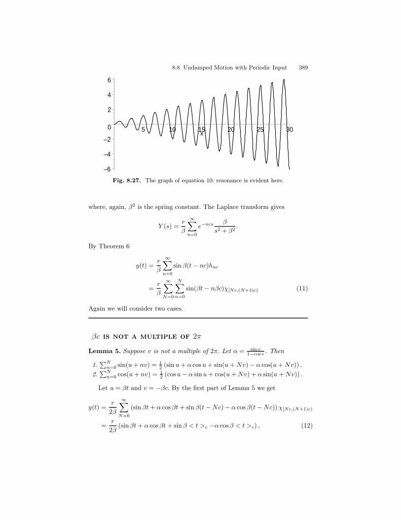
8.8 Undamped Motion with Periodic Input 389
–6
–4
–2
0
2
4
6
5 10 15 20 25 30x
Fig. 8.27. The graph of equation 10: resonance is evident here.
where, again, β2 is the spring constant. The Laplace transform gives
Y (s) =r
β
∞∑
n=0
e−ncs β
s2 + β2.
By Theorem 6
y(t) =r
β
∞∑
n=0
sinβ(t− nc)hnc
=r
β
∞∑
N=0
N∑
n=0
sin(βt− nβc)χ[Nc,(N+1)c) (11)
Again we will consider two cases.
βc is not a multiple of 2π
Lemma 5. Suppose v is not a multiple of 2π. Let α = sin v1−cos v . Then
1.∑N
n=0 sin(u+ nv) = 12 (sinu+ α cosu+ sin(u+Nv)− α cos(u+Nv)) .
2.∑N
n=0 cos(u+ nv) = 12 (cosu− α sinu+ cos(u+Nv) + α sin(u+Nv)) .
Let u = βt and v = −βc. By the first part of Lemma 5 we get
y(t) =r
2β
∞∑
N=0
(sinβt+ α cosβt+ sinβ(t−Nc)− α cosβ(t−Nc))χ[Nc,(N+1)c)
=r
2β(sinβt+ α cosβt+ sinβ < t >c −α cosβ < t >c) , (12)
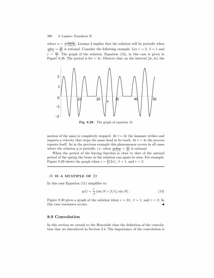
390 8 Laplace Transform II
where α = − sin βc1−cos βc . Lemma 3 implies that the solution will be periodic when
c2π/β = βc
2π is rational. Consider the following example. Let r = 2, β = 1 and
c = 3π2 . The graph of the solution, Equation (12), in this case is given in
Figure 8.28. The period is 6π = 4c. Observe that on the interval [3c, 4c) the
–2
–1
0
1
2
10 20 30 40 50x
Fig. 8.28. The graph of equation 12
motion of the mass is completely stopped. At t = 3c the hammer strikes andimparts a velocity that stops the mass dead in its track. At t = 4c the processrepeats itself. As in the previous example this phenomenon occurs in all caseswhere the solution y is periodic, i.e. when c
2π/(β) = βc2π is rational.
When the period of the forcing function is close to that of the naturalperiod of the spring the beats in the solution can again be seen. For example,Figure 8.29 shows the graph when c = 9
8 (2π), β = 1, and r = 2.
βc is a multiple of 2π
In this case Equation (11) simplifies to
y(t) =r
β(sinβt+ [t/c]1 sinβt) . (13)
Figure 8.30 gives a graph of the solution when c = 2π, β = 1, and r = 2. Inthis case resonance occurs. J
8.9 Convolution
In this section we extend to the Heaviside class the definition of the convolu-tion that we introduced in Section 3.4. The importance of the convolution is
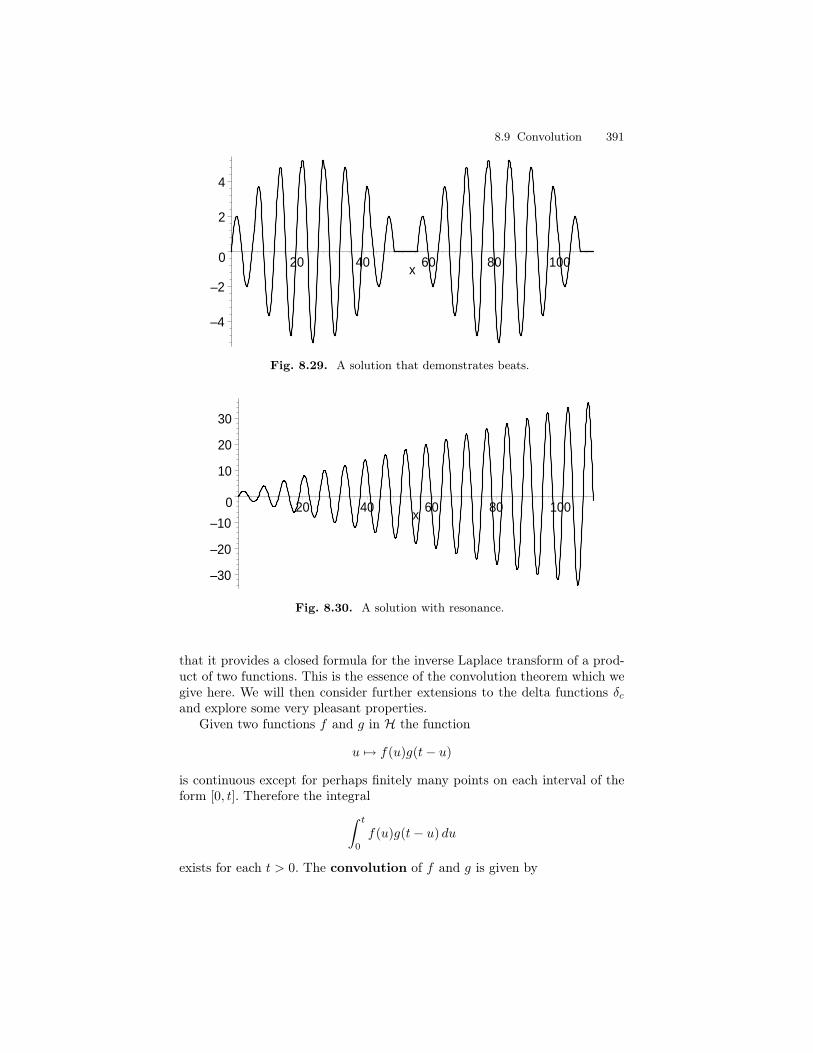
8.9 Convolution 391
–4
–2
0
2
4
20 40 60 80 100x
Fig. 8.29. A solution that demonstrates beats.
–30
–20
–10
0
10
20
30
20 40 60 80 100x
Fig. 8.30. A solution with resonance.
that it provides a closed formula for the inverse Laplace transform of a prod-uct of two functions. This is the essence of the convolution theorem which wegive here. We will then consider further extensions to the delta functions δcand explore some very pleasant properties.
Given two functions f and g in H the function
u 7→ f(u)g(t− u)
is continuous except for perhaps finitely many points on each interval of theform [0, t]. Therefore the integral
∫ t
0
f(u)g(t− u) du
exists for each t > 0. The convolution of f and g is given by
392 8 Laplace Transform II
f ∗ g(t) =
∫ t
0
f(u)g(t− u) du.
We will not make the argument but it can be shown that f ∗ g is in factcontinuous. Since there are numbers K, L, a, and b such that
|f(t)| ≤ Keat and |g(t)| ≤ Lebt
it follows that
|f ∗ g(t)| ≤∫ t
0
|f(u)| |g(t− u)| du
≤ KL
∫ t
0
eaueb(t−u) du
= KLebt
∫ t
0
e(a−b)u du
= KL
tebt if a = beat−ebt
a−b if a 6= b.
This shows that f ∗ g is of exponential type and therefore is back in H.The linearity properties we listed in Section 3.4 extend to H. We restate
them here: Suppose f , g, and h are in H. Then
1. f ∗ g ∈ H2. f ∗ g = g ∗ f3. (f ∗ g) ∗ h = f ∗ (g ∗ h)4. f ∗ (g + h) = f ∗ g + f ∗ h5. f ∗ 0 = 0.
The sliding window and an example
Let’s now break the convolution up into its constituents to get a better ideaof what it does. The function u 7→ g(−u) has a graph that is folded or flippedacross the y-axis. The function u 7→ g(t − u) shifts the flip by t ≥ 0. Theconvolution measures the amount of overlap between f and the flip and shiftof g by positive values t. One can think of g(t − u) as a horizontally slidingwindow by which f is examined and measured.
Example 1. Let f(t) = tχ[0,1)(t) and g(t) = χ[1,2)(t). Find the convolutionf ∗ g.
I Solution. The flip of g is g(−u) = χ[−2,−1)(u) while the flip and shift ofg is g(t− u) = χ[t−2,t−1)(u). See Figure 8.31.
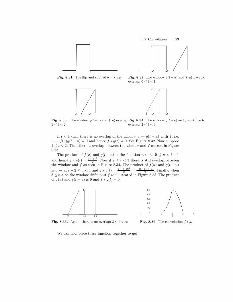
8.9 Convolution 393
t–1t–2
Fig. 8.31. The flip and shift of g = χ[1,2).
1
t–1t–2 0
Fig. 8.32. The window g(t− u) and f(u) have nooverlap: 0 ≤ t < 1
1
0 t–1t–2
Fig. 8.33. The window g(t−u) and f(u) overlap:1 ≤ t < 2.
t–2 t–10
1
Fig. 8.34. The window g(t−u) and f continue tooverlap: 2 ≤ t < 3.
If t < 1 then there is no overlap of the window u 7→ g(t − u) with f , i.e.u 7→ f(u)g(t− u) = 0 and hence f ∗ g(t) = 0. See Figure 8.32. Now suppose1 ≤ t < 2. Then there is overlap between the window and f as seen in Figure8.33.
The product of f(u) and g(t − u) is the function u 7→ u, 0 ≤ u < t − 1
and hence f ∗ g(t) = (t−1)2
2 . Now if 2 ≤ t < 3 there is still overlap betweenthe window and f as seen in Figure 8.34. The product of f(u) and g(t − u)is u 7→ u, t− 2 ≤ u < 1 and f ∗ g(t) = 1−(t−2)2
2 = −(t−1)(t−3)2 . Finally, when
3 ≤ t <∞ the window shifts past f as illustrated in Figure 8.35. The productof f(u) and g(t− u) is 0 and f ∗ g(t) = 0.
0 t–1
1
t–2
Fig. 8.35. Again, there is no overlap: 3 ≤ t < ∞
0
0.1
0.2
0.3
0.4
0.5
–1 1 2 3 4t
Fig. 8.36. The convolution f ∗ g.
We can now piece these function together to get
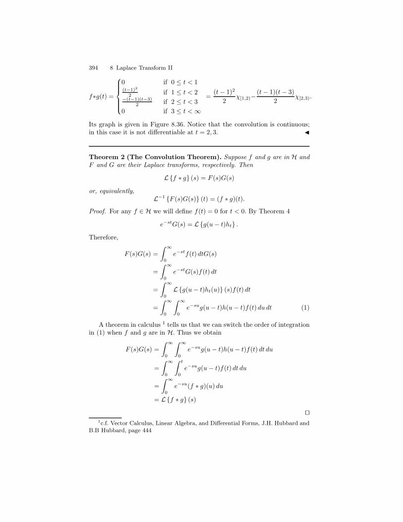
394 8 Laplace Transform II
f∗g(t) =
0 if 0 ≤ t < 1(t−1)2
2 if 1 ≤ t < 2−(t−1)(t−3)
2 if 2 ≤ t < 3
0 if 3 ≤ t <∞
=(t− 1)2
2χ[1,2)−
(t− 1)(t− 3)
2χ[2,3).
Its graph is given in Figure 8.36. Notice that the convolution is continuous;in this case it is not differentiable at t = 2, 3. J
Theorem 2 (The Convolution Theorem). Suppose f and g are in H andF and G are their Laplace transforms, respectively. Then
Lf ∗ g (s) = F (s)G(s)
or, equivalently,L−1 F (s)G(s) (t) = (f ∗ g)(t).
Proof. For any f ∈ H we will define f(t) = 0 for t < 0. By Theorem 4
e−stG(s) = Lg(u− t)ht .
Therefore,
F (s)G(s) =
∫ ∞
0
e−stf(t) dtG(s)
=
∫ ∞
0
e−stG(s)f(t) dt
=
∫ ∞
0
Lg(u− t)ht(u) (s)f(t) dt
=
∫ ∞
0
∫ ∞
0
e−sug(u− t)h(u− t)f(t) du dt (1)
A theorem in calculus 1 tells us that we can switch the order of integrationin (1) when f and g are in H. Thus we obtain
F (s)G(s) =
∫ ∞
0
∫ ∞
0
e−sug(u− t)h(u− t)f(t) dt du
=
∫ ∞
0
∫ t
0
e−sug(u− t)f(t) dt du
=
∫ ∞
0
e−su(f ∗ g)(u) du
= Lf ∗ g (s)
ut1c.f. Vector Calculus, Linear Algebra, and Differential Forms, J.H. Hubbard and
B.B Hubbard, page 444
8.9 Convolution 395
There are a variety of uses for the convolution theorem. For one it issometimes a convenient way to compute the convolution of two functions fand g; namely (f ∗ g)(t) = L−1 F (s)G(s) .
Example 3. Compute the convolution of the functions given in 1:
f(t) = tχ[0,1) and g(t) = χ[1,2).
In the following example, which is a reworking of Example 1, instead of keepingtrack of the sliding window g(t−u) the convolution theorem turns the probleminto one that is primarily algebraic.
I Solution. The Laplace transforms of f and g are, respectively,
F (s) =1
s2− e−s
(
1
s2+
1
s
)
and G(s) =e−s − e−2s
s.
The product simplifies to
F (s)G(s) =1
s3e−s −
(
2
s3+
1
s2
)
e−2s +
(
1
s3+
1
s2
)
e−3s.
Its inverse Laplace transform is
(f ∗ g)(t) = L−1 F (s)G(s) (t)
=(t− 1)2
2h1(t)− ((t− 2)(t− 1))h2(t) +
(t− 3)(t− 1)
2h3(t)
=(t− 1)2
2χ[1,2)(t)−
(t− 1)(t− 3)
2χ[2,3)(t)
J
Convolution and the Dirac Delta Function
We would like to extend the definition of convolution to include the deltafunctions δc, c ≥ 0. Recall that we formally defined the delta function by
δc(t) = limε→0
dc,ε(t),
where dc,ε = 1εχ[c,c+ε). In like manner, for f ∈ H, we define
f ∗ δc(t) = limε→0
f ∗ dc,ε(t).
396 8 Laplace Transform II
Theorem 4. For f ∈ H
f ∗ δc(t) = f(t− c)hc,
where the equality is understood to mean essentially equal.
Proof. Let f ∈ H. Then
f ∗ dc,ε(t) =
∫ t
0
f(u)dc,ε(t− u) dt
=1
ε
∫ t
0
f(u)χ[c,c+ε)(t− u) du
=1
ε
∫ t
0
f(u)χ[t−c−ε,t−c)(u) du
Now suppose t < c. Then χ[t−c−ε,t−c)(u) = 0, for all u ∈ [0, t). Thus f ∗dc,ε =0. On the other hand if t > c then for ε small enough we have
f ∗ dc,ε(t) =1
ε
∫ t−c
t−c−ε
f(u) du.
Let t be such that t−c is a point of continuity of f . Then by the FundamentalTheorem of Calculus
limε→0
1
ε
∫ t−c
t−c−ε
f(u) du = f(t− c).
Since f has only finitely many removable discontinuities on any finite intervalit follows that f ∗ δc is essentially equal to f(t− c)hc. ut
The special case c = 0 produces the following pleasant corollary.
Corollary 5. For f ∈ H we have
f ∗ δ0 = f.
This corollary tells us that this extension to the Dirac delta function givesan identity under the convolution product. We thus have a correspondencebetween the multiplicative identities in domain and transform space underthe Laplace transform since Lδ0 = 1.
The Impulse Response Function
Let f ∈ H. Let us return to our basic second order differential equation
ay′′ + by′ + cy = f(t), y(0) = y0 and y′(0) = y1. (2)
8.9 Convolution 397
By organizing terms in its Laplace transform in the right manner we canexpress the solution in terms of convolution of a special function called theimpulse response function and f . To explain the main idea let’s begin byconsidering the following special case
ay′′ + by′ + cy = 0 y(0) = 0 and y′(0) = 1.
This corresponds to a system in initial position but with a unit velocity. Ourdiscussion in Section 8.6 shows that this is exactly the same thing as solving
ay′′ + by′ + cy = δ0, y(0) = 0 and y′(0) = 0
the same system at rest but with unit impulse at t = 0. The Laplace transformof either equation above leads to
Y (s) =1
as2 + bs+ c.
The inverse Laplace transform is the solution and will be denoted by ζ(t); itis called the impulse response function.
The Laplace transform of Equation 2 leads to
Y (s) =(as+ b)y0 + y1as2 + bs+ c
+F (s)
as2 + bs+ c.
Let
H(s) =(as+ b)y0 + y1as2 + bs+ c
and G(s) =F (s)
as2 + bs+ c.
Then Y (s) = H(s) + G(s). The inverse Laplace transform of H correspondsto the solution to Equation 2 when f = 0. It is the homogeneous solution. Onthe other hand, G can be written as a product
G(s) = F (s)
(
1
as2 + bs+ c
)
and its inverses Laplace transform g(t) is
g(t) = f ∗ ζ(t),
by the convolution theorem.We summarize this discussion in the following theorem:
Theorem 6. Let f ∈ H. The solution to Equation 2 can be expressed as
h(t) + f ∗ ζ(t),
where h is the homogenous solution to Equation 2 and ζ is the impulse re-sponse function.
398 8 Laplace Transform II
Example 7. Solve the following differential equation:
y′′ + 4y = χ[0,1) y(0) = 0 and y′(0) = 0.
I Solution. The homogeneous solution to
y′′ + 4y = 0 y(0) = 0 and y′(0) = 0
is the trivial solution h = 0. The impulse response function is
ζ(t) = L−1
1
s2 + 4
=1
2sin 2t.
By Theorem 6 the solution is
y(t) = ζ ∗ χ[0,1)
=
∫ t
0
1
2sin(2u)χ[0,1)(t− u) du
=1
2
∫ t
0
sin(2u)χ[t− 1, t)(u) du
=1
2
∫ t
0sin 2u du if 0 ≤ t < 1
∫ t
t−1 sin 2u du if 1 ≤ u <∞
=1
4
1− cos 2t if 0 ≤ t < 1
cos 2(t− 1)− cos 2t if 1 ≤ t <∞
J
9
Matrices
Most students by now have been exposed to the language of matrices. Theyarise naturally in many subject areas but mainly in the context of solvinga simultaneous system of linear equations. In this chapter we will give a re-view of matrices, systems of linear equations, inverses, and determinants. Thenext chapter will apply what is learned here to linear systems of differentialequations.
9.1 Matrix Operations
A matrix is a rectangular array of entities and is generally written in thefollowing way:
X =
x11 · · · x1n
.... . .
...xm1 · · · xmn
.
We let R denote the set of entities that will be in use at any particular time.Each xij is in R and in this text R can be one of the following sets:
R or C The scalarsR[t] or C[t] Polynomials with real or complex entriesR(s) or C(s) The real or complex rational functionsCn(I,R) or Cn(I,C) Real or complex valued functions
with n continuous derivatives
Notice that addition and scalar multiplication is defined on R. Below we willextend these operations to matrices. (In Chapter 10 we will see an instancewhere R will even be matrices themselves; thus matrices of matrices. But wewill avoid that for now.)
The following are examples of matrices.
400 9 Matrices
Example 1.
A =
[
1 0 32 −1 4
]
B =[
1 −1 9]
C =
[
i 2− i1 0
]
D =
[
t2e2t
t3 cos t
]
E =
[ ss2−1
1s2−1
−1s2−1
s+2s2−1
]
It is a common practice to use capital letters, like A, B, C, D, and E, todenote matrices. The size of a matrix is determined by the number of rowsm and the number of columns n and written m × n. In Example 1 A is a2 × 3 matrix, B is a 1 × 3 matrix, C and E are 2 × 2 matrices, and D is a2 × 1 matrix. A matrix is square if the number of rows is the same as thenumber of columns. Thus, C and E are square matrices. An entry in a matrixis determined by its position. If X is a matrix the (i, j) entry is the entry thatappears in the ith row and jth column. We denote it in two ways: entij(X)or more simply Xij . Thus, in Example 1, A1 3 = 3, B1 2 = −1, and C2 2 = 0.We say that two matrices X and Y are equal if the corresponding entries areequal, i.e. Xi j = Yi j , for all indices i and j. Necessarily X and Y must bethe same size. The main diagonal of a square n× n matrix X is the vectorformed from the entries Xi i, for i = 1, . . . , n. The main diagonal of C is (i, 0)and the main diagonal of E is ( s
s2−1 ,s+2s2−1 ). In this book all scalars are either
real or complex. A matrix is said to be a real matrix if each entry is realand a complex matrix if each entry is complex. Since every real number isalso complex, every real matrix is also a complex matrix. Thus A and B arereal ( and complex) matrices while C is a complex matrix.
Even though a matrix is a structured array of entities in R it should beviewed as a single object just as a word is a single object though made upof many letters. We let Mm,n(R) denote the set of all m × n matrices withentries in R. If the focus is on matrices of a certain size and not the entrieswe will sometimes just write Mm,n.
The following definitions highlights various kinds of matrices that com-monly arise.
1. A diagonal matrix D is a square matrix in which all entries off the maindiagonal are 0. We can say this in another way:
Di j = 0 if i 6= j.
Examples of diagonal matrices are:
[
1 00 4
]
et 0 00 e4t 00 0 1
1s 0 0 00 2
s−1 0 0
0 0 0 00 0 0 − 1
s−2
.
It is convenient to write diag(d1, . . . , dn) to represent the diagonal n× nmatrix with (d1, . . . , dn) on the diagonal. Thus the diagonal matrices
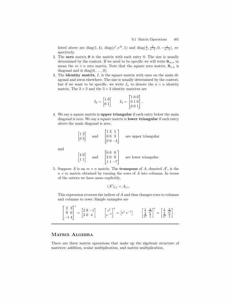
9.1 Matrix Operations 401
listed above are diag(1, 4), diag(et, e4t, 1) and diag(1s ,
2s−1 , 0,− 1
s−2 ), re-spectively.
2. The zero matrix 0 is the matrix with each entry 0. The size is usuallydetermined by the context. If we need to be specific we will write 0m,n tomean the m × n zero matrix. Note that the square zero matrix, 0n,n isdiagonal and is diag(0, . . . , 0).
3. The identity matrix, I, is the square matrix with ones on the main di-agonal and zeros elsewhere. The size is usually determined by the context,but if we want to be specific, we write In to denote the n × n identitymatrix. The 2× 2 and the 3× 3 identity matrices are
I2 =
[
1 00 1
]
I3 =
1 0 00 1 00 0 1
.
4. We say a square matrix is upper triangular if each entry below the maindiagonal is zero. We say a square matrix is lower triangular if each entryabove the main diagonal is zero.
[
1 20 3
]
and
1 3 50 0 30 0 −4
are upper triangular
and[
4 01 1
]
and
0 0 02 0 01 1 −7
are lower triangular.
5. Suppose A is an m × n matrix. The transpose of A, denoted At, is then ×m matrix obtained by turning the rows of A into columns. In termsof the entries we have more explicitly,
(At)i j = Aj i.
This expression reverses the indices of A and thus changes rows to columnsand columns to rows. Simple examples are
2 39 0−1 4
t
=
[
2 9 −13 0 4
] [
et
e−t
]t
=[
et e−t]
[
1s
2s3
2s2
3s
]t
=
[
1s
2s2
2s3
3s
]
.
Matrix Algebra
There are three matrix operations that make up the algebraic structure ofmatrices: addition, scalar multiplication, and matrix multiplication.
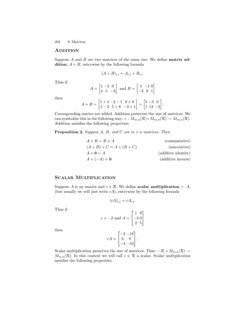
402 9 Matrices
Addition
Suppose A and B are two matrices of the same size. We define matrix ad-dition, A+B, entrywise by the following formula
(A+B)i j = Ai j +Bi j .
Thus if
A =
[
1 −2 04 5 −3
]
and B =
[
4 −1 0−3 8 1
]
then
A+B =
[
1 + 4 −2− 1 0 + 04− 3 5 + 8 −3 + 1
]
=
[
5 −3 01 13 −2
]
.
Corresponding entries are added. Addition preserves the size of matrices. Wecan symbolize this in the following way: + : Mm,n(R)×Mm,n(R)→Mm,n(R).Addition satisfies the following properties:
Proposition 2. Suppose A, B, and C are m× n matrices. Then
A+B = B +A (commutative)
(A+B) + C = A+ (B + C) (associative)
A+ 0 = A (additive identity)
A+ (−A) = 0 (additive inverse)
Scalar Multiplication
Suppose A is an matrix and c ∈ R. We define scalar multiplication, c · A,(but usually we will just write cA), entrywise by the following formula
(cA)i j = cAi j .
Thus if
c = −2 and A =
1 9−3 02 5
then
cA =
−2 −186 0−4 −10
.
Scalar multiplication preserves the size of matrices. Thus · : R×Mm,n(R)→Mm,n(R). In this context we will call c ∈ R a scalar. Scalar multiplicationsatisfies the following properties:
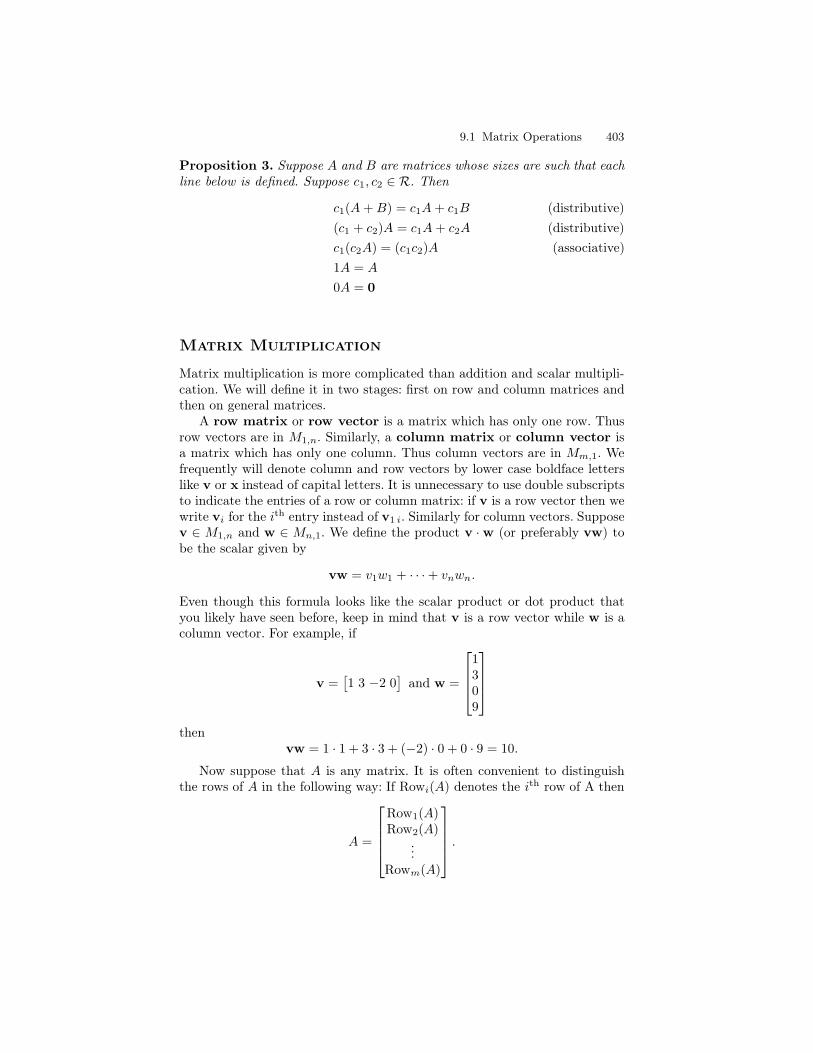
9.1 Matrix Operations 403
Proposition 3. Suppose A and B are matrices whose sizes are such that eachline below is defined. Suppose c1, c2 ∈ R. Then
c1(A+B) = c1A+ c1B (distributive)
(c1 + c2)A = c1A+ c2A (distributive)
c1(c2A) = (c1c2)A (associative)
1A = A
0A = 0
Matrix Multiplication
Matrix multiplication is more complicated than addition and scalar multipli-cation. We will define it in two stages: first on row and column matrices andthen on general matrices.
A row matrix or row vector is a matrix which has only one row. Thusrow vectors are in M1,n. Similarly, a column matrix or column vector isa matrix which has only one column. Thus column vectors are in Mm,1. Wefrequently will denote column and row vectors by lower case boldface letterslike v or x instead of capital letters. It is unnecessary to use double subscriptsto indicate the entries of a row or column matrix: if v is a row vector then wewrite vi for the ith entry instead of v1 i. Similarly for column vectors. Supposev ∈ M1,n and w ∈ Mn,1. We define the product v ·w (or preferably vw) tobe the scalar given by
vw = v1w1 + · · ·+ vnwn.
Even though this formula looks like the scalar product or dot product thatyou likely have seen before, keep in mind that v is a row vector while w is acolumn vector. For example, if
v =[
1 3 −2 0]
and w =
1309
thenvw = 1 · 1 + 3 · 3 + (−2) · 0 + 0 · 9 = 10.
Now suppose that A is any matrix. It is often convenient to distinguishthe rows of A in the following way: If Rowi(A) denotes the ith row of A then
A =
Row1(A)Row2(A)
...Rowm(A)
.
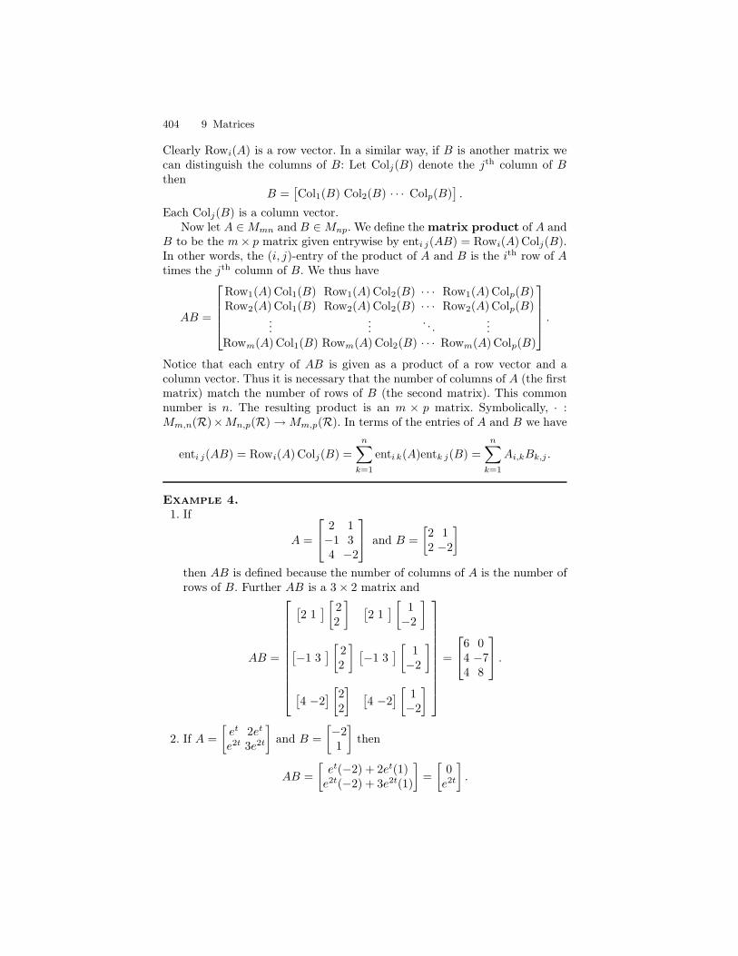
404 9 Matrices
Clearly Rowi(A) is a row vector. In a similar way, if B is another matrix wecan distinguish the columns of B: Let Colj(B) denote the jth column of Bthen
B =[
Col1(B) Col2(B) · · · Colp(B)]
.
Each Colj(B) is a column vector.Now let A ∈Mmn and B ∈Mnp. We define the matrix product of A and
B to be the m× p matrix given entrywise by enti j(AB) = Rowi(A)Colj(B).In other words, the (i, j)-entry of the product of A and B is the ith row of Atimes the jth column of B. We thus have
AB =
Row1(A)Col1(B) Row1(A)Col2(B) · · · Row1(A)Colp(B)Row2(A)Col1(B) Row2(A)Col2(B) · · · Row2(A)Colp(B)
......
. . ....
Rowm(A)Col1(B) Rowm(A)Col2(B) · · · Rowm(A)Colp(B)
.
Notice that each entry of AB is given as a product of a row vector and acolumn vector. Thus it is necessary that the number of columns of A (the firstmatrix) match the number of rows of B (the second matrix). This commonnumber is n. The resulting product is an m × p matrix. Symbolically, · :Mm,n(R)×Mn,p(R)→Mm,p(R). In terms of the entries of A and B we have
enti j(AB) = Rowi(A)Colj(B) =
n∑
k=1
enti k(A)entk j(B) =
n∑
k=1
Ai,kBk,j .
Example 4.1. If
A =
2 1−1 34 −2
and B =
[
2 12 −2
]
then AB is defined because the number of columns of A is the number ofrows of B. Further AB is a 3× 2 matrix and
AB =
[
2 1]
[
22
]
[
2 1]
[
1−2
]
[
−1 3]
[
22
]
[
−1 3]
[
1−2
]
[
4 −2]
[
22
]
[
4 −2]
[
1−2
]
=
6 04 −74 8
.
2. If A =
[
et 2et
e2t 3e2t
]
and B =
[
−21
]
then
AB =
[
et(−2) + 2et(1)e2t(−2) + 3e2t(1)
]
=
[
0e2t
]
.
9.1 Matrix Operations 405
Notice in the definition (and the example) that in a given column of ABthe corresponding column of B appears as the second factor. Thus
Colj(AB) = AColj(B). (1)
Similarly, in each row of AB the corresponding row of A appears and we get
Rowi(A)B = Rowi(AB). (2)
Notice too that even though the product AB is defined it is not necessarilytrue that BA is defined. This is the case in part 1 of the above example dueto the fact that the number of columns of B (2) does not match the numberof rows of A (3). Even when AB and BA are defined it is not necessarily truethat they are equal. Consider the following example:
Example 5. Suppose
A =
[
1 20 3
]
and B =
[
2 14 −1
]
.
Then
AB =
[
1 20 3
] [
2 14 −1
]
=
[
10 −112 −3
]
yet
BA =
[
2 14 −1
] [
1 20 3
]
=
[
2 74 5
]
.
These products are not the same. This example show that matrix multiplica-tion is not commutative. However, the other properties that we are used toin an algebra are valid. We summarize them in the following proposition.
Proposition 6. Suppose A, B, and C are matrices whose sizes are such thateach line below is defined. Suppose c1, c2 ∈ R. Then
A(BC) = (AB)C (associatvie)
A(c1B) = (c1A)B = c1(AB) (associative)
(A+B)C = AC +BC (distributive)
A(B + C) = AB +AC (distributive)
IA = AI = I (I is a multiplicative identity)
We highlight two useful formulas that follow from these algebraic proper-ties. If A is an m× n matrix then
Ax = x1 Col1(A) + · · ·xn Coln(A), where x =
x1
...xn
(3)
406 9 Matrices
and
yA = y1Row1(A) + · · · ymRowm(A), where y =[
y1 · · · ym
]
. (4)
Henceforth, we will use these algebraic properties without explicit refer-ence. The following result expresses the relationship between multiplicationand transposition of matrices
Theorem 7. Let A and B be matrices such that AB is defined. Then BtAt
is defined andBtAt = (AB)t.
Proof. The number of columns of Bt is the same as the number of rows ofB while the number of rows of At is the number of columns of A. Thesenumbers agree since AB is defined so BtAt is defined. If n denotes thesecommon numbers then
(BtAt)i j =n∑
k=1
(Bt)i k(At)k j =n∑
k=1
Aj kBk i = (AB)j i = ((AB)t)i j .
ut
Exercises
Let A = 2 −1 31 0 4, B = 1 −1
2 3−1 2 , and C = 0 2
−3 41 1. Compute the following
matrices.
1. B + C, B − C, 2B − 3C
2. AB, AC, BA, CA
3. A(B + C), AB + AC, (B + C)A
4. Let A = 2 13 4−1 0 and B = 1 2
−1 11 0. Find C so that 3A + C = 4B.
Let A = 3 −10 −21 2 , B = 2 1 1 −3
0 −1 4 −1, and C =2 1 21 3 10 1 81 1 7
. Find the following
products
5. AB
6. BC
9.1 Matrix Operations 407
7. CA
8. BtAt
9. ABC.
10. Let A = 1 4 3 1! and B =1
0−1−2
. Find AB and BA.
Let A = 1 2 52 4 10−1 −2 −5, B = 1 0
4 −1, C = 3 −23 −2. Verify the following facts:
11. A2 = 0
12. B2 = I2
13. C2 = C
Compute AB − BA in each of the following cases.
14. A = 0 11 1, B = 1 0
1 115. A = 2 1 0
1 1 1−1 2 1, B = 3 1 −2
3 −2 4−3 5 −1
16. Let A = 1 a0 1 and B = 1 0
b 1. Show that there are no numbers a and b so that
AB − BA = I , where I is the 2 × 2 identity matrix.
17. Suppose that A and B are 2 × 2 matrices.a) Show by example that it need not be true that (A+B)2 = A2 +2AB +B2.b) Find conditions on A and B to insure that the equation in Part (a) is valid.
18. If A = 0 11 1, compute A2 and A3.
19. If B = 1 10 1, compute Bn for all n.
20. If A = a 00 b, compute A2, A3, and more generally, An for all n.
21. Let A = v1
v2 be a matrix with two rows v1 and v2. (The number of columns of
A is not relevant for this problem) Describe the effect of multiplying A on theleft by the following matrices:
(a) 0 11 0 (b) 1 c
0 1 (c) 1 0c 1 (d) a 0
0 1 (e) 1 00 a
408 9 Matrices
22. Let E(θ) = cos θ sin θ− sin θ cos θ. Show that E(θ1 + θ2) = E(θ1)E(θ2).
23. Let (θ) = cosh θ sinh θsinh θ cosh θ. Show that F (θ1 + θ2) = F (θ1)F (θ2).
24. Let D = diag(d1, . . . , dn) and E = diag(e1, . . . , e2). Show that
DE = diag(d1e1, . . . , dnen)
.
9.2 Systems of Linear Equations
Most students have learned various techniques for finding the solution of asystem of linear equations. They usually include various forms of eliminationand substitutions. In this section we will learn the Gauss-Jordan eliminationmethod. It is essentially a highly organized method involving elimination andsubstitution that always leads to the solution set. This general method hasbecome the standard for solving systems. At first reading it may seem to bea bit complicated because of its description for general systems. However,with a little practice on a few examples it is quite easy to master. We willas usual begin with our definitions and proceed with examples to illustratethe needed concepts. To make matters a bit cleaner we will stick to the casewhere R = R. Everything we do here will work for R = C , R(s), or C(s) aswell. (A technical difficulty for general R is the lack of inverses.)
If x1, . . . , xn are variables then the equation
a1x1 + · · ·+ anxn = b
is called a linear equation in the unknowns x1, . . . , xn. A system of linearequations is a set of m linear equations in the unknowns x1, . . . , xn and iswritten in the form
a1 1x1 + a1 2x2 + · · · + a1 nxn = b1a2 1x1 + a2 2x2 + · · · + a2 nxn = b2
......
......
am 1x1 + am 2x2 + · · · + am nxn = bm.
(1)
The entries ai j are in R and are called coefficients. Likewise, each bj isin R. A key observation is that Equation (1) can be rewritten in matrix formas:
Ax = b, (2)
where
9.2 Systems of Linear Equations 409
A =
a1 1 a1 2 · · · a1 n
a2 1 a2 2 · · · a2 n
......
...am 1 am 2 · · · am n,
x =
x1
x2
...xn
and b =
b1b2...bm
.
We call A the coefficient matrix, x the variable matrix, and b theoutput matrix. Any column vector x with entries in R that satisfies (1) (or(2)) is called a solution. If a system has a solution we say it is consistent;otherwise, it is inconsistent. The solution set, denoted by Sb
A, is the set ofall solutions. The system (1) is said to be homogeneous if b = 0, otherwiseit is called nonhomogeneous. Another important matrix associated with (2)is the augmented matrix:
[A| b ] =
a1 1 a1 2 · · · a1 n b1a2 1 a2 2 · · · a2 n b2
......
......
am 1 am 2 · · · am n bm
,
where the vertical line only serves to separate A from b.
Example 1. Write the coefficient, variable, output, and augmented matricesfor the following system:
−2x1 + 3x2 − x3 = 4x1 − 2x2 + 4x3 = 5.
Determine whether the following vectors are solutions:
(a) x =
−302
(b) x =
773
(c) x =
1071
(d) x =
[
21
]
.
I Solution. The coefficient matrix is A =
[
−2 3 −11 −2 4
]
, the variable matrix
is x =
x1
x2
x3
, the output matrix is b =
[
45
]
, and the augmented matrix is
[
−2 3 −1 41 −2 4 5
]
. The system is nonhomogeneous. Notice that
A
−302
=
[
45
]
and A
773
=
[
45
]
while A
1071
=
[
00
]
.
Therefore (a) and (b) are solutions, (c) is not a solution and the matrix in (d)is not the right size and thus cannot be a solution. J
410 9 Matrices
Remark 2. When only 2 or 3 variables are involved in an example we willfrequently use the variables x, y, and z instead of the subscripted variablesx1, x2, and x3.
Linearity
It is convenient to think of Rn as the set of column vectors Mn,1(R). If A isan m× n real matrix then for each column vector x ∈ Rn, the product, Ax,is a column vector in Rm. Thus the matrix A induces a map which we alsodenote just by A : Rn → Rm given by matrix multiplication. It satisfies thefollowing important property.
Proposition 3. The map A : Rn → Rm is linear. In other words,
1. A(x + y) = A(x) +A(y)2. A(cx) = cA(x),
for all x,y ∈ Rn and c ∈ R.
Proof. This follows directly from Propositions 3 and 6. ut
Linearity is an extremely important property for it allows us to describethe structure of the solution set to Ax = b in a particularly nice way. Recallthat Sb
A denotes the solution set to the equation Ax = b.
Proposition 4. With A as above we have two possibilities:
1. SbA = ∅ or
2. there is an xp ∈ SbA and Sb
A = xp + S0A.
In other words, when SbA is not the empty set then each solution to Ax = b
has the formxp + xh,
where xp is a fixed particular solution to Ax = b and xh is a solution toAx = 0.
Proof. Suppose xp is a fixed particular solution and xh ∈ S0A. Then A(xp +
xh) = Axp + Axh = b + 0 = b. This implies that each column vector ofthe form xp + xh is in Sb
A. On the other hand, suppose x is in SbA. Then
A(x − xp) = Ax − Axp = b − b = 0. This means that x − xp is in S0A.
Therefore x = xp + xh, for some vector xh ∈ S0A. ut
Remark 5. The system of equations Ax = 0 is called the associated ho-mogeneous system. Case (1) is a legitimate possibility. For example, thesimple equation 0x = 1 has empty solution set. When the solution set is notempty it should be mentioned that the particular solution xp is not necessarily
9.2 Systems of Linear Equations 411
unique. In Chapter 6 we saw a similar theorem for a second order differentialequation Ly = f . That theorem provided a strategy for solving such differen-tial equations: First we solved the homogeneous equation Ly = 0 and secondfound a particular solution (using variation of parameters or undeterminedcoefficients). For a linear system of equations the matter is much simpler; theGauss-Jordan method will give the whole solution set at one time. We willsee that it has the above form.
Homogenous Systems
The homogeneous case, Ax = 0, is of particular interest. Observe that x = 0
is always a solution so S0A is never the empty set, i.e. case (1) is not possible.
But much more is true.
Proposition 6. The solution set, S0A, to a homogeneous system is closed un-
der addition and multiplication by scalars. In other words, if x and y aresolutions to the homogeneous system and c is a scalar then x + y and cx arealso solutions.
Proof. Suppose x and y are in S0A. Then A(x + y) = Ax +Ay = 0 + 0 = 0.
This shows that x + y is in S0A. Now suppose c ∈ R. Then A(cx) = cAx =
c0 = 0. Hence cx ∈ S0A. This shows that S0
A is closed under addition andscalar multiplication. ut
Corollary 7. The solution set to a general system of linear equations, Ax =b, is either
1. empty2. unique3. or infinite.
Proof. The associated homogeneous system Ax = 0 has solution set, S0A, that
is either equal to the trivial set 0 or an infinite set. To see this suppose thatx is a nonzero solution to Ax = 0 then by Proposition 6 all multiples, cx, arein S0
A as well. Therefore, by Proposition 4, if there is a solution to Ax = b itis unique or there are infinitely many. ut
The Elementary Equation and Row Operations
We say that two systems of equations are equivalent if their solution setsare the same. This definition implies that the variable matrix is the same foreach system.
412 9 Matrices
Example 8. Consider the following systems of equations:
2x + 3y = 5x − y = 0
andx = 1y = 1.
The solution set to the second system is transparent. For the first system thereare some simple operations that easily lead to the solution: First, switch thetwo equations around. Next, multiply the equation x− y = 1 by −2 and addthe result to the first. We then obtain
x − y = 05y = 5
Next, multiply the second equation by 15 to get y = 1. Then add this equation
to the first. We get x = 1 and y = 1. Thus they both have the same solution
set, namely the single vector
[
11
]
. They are thus equivalent. When used in
the right way these kinds of operations can transform a complicated systeminto a simpler one. We formalize these operations in the following definition:
Suppose Ax = b is a given system of linear equations. The following threeoperations are called elementary equation operations.
1. Switch the order in which two equations are listed2. Multiply an equation by a nonzero scalar3. Add a multiple of one equation to another
Notice that each operation produces a new system of linear equations butleaves the size of the system unchanged. Furthermore we have the followingproposition.
Proposition 9. An elementary equation operation applied to a system of lin-ear equations is an equivalent system of equations.
Proof. This means that the system that arises from an elementary equationoperation has the same solution set as the original. We leave the proof as anexercise. ut
The main idea in solving a system of linear equations is to perform afinite sequence of elementary equation operations to transform a system intosimpler system where the solution set is transparent. Proposition 9 impliesthat the solution set of the simpler system is the same as original system.Let’s consider our example above.
Example 10. Use elementary equation operations to transform
2x + 3y = 5x − y = 0
intox = 1y = 1.
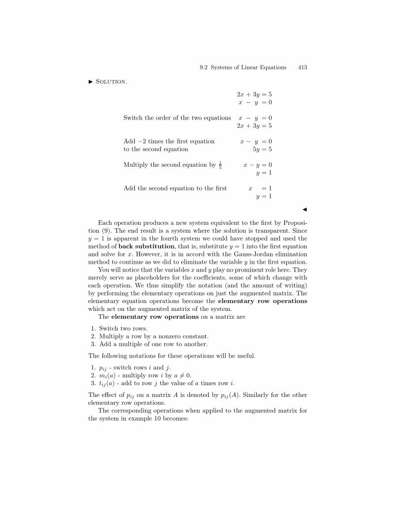
9.2 Systems of Linear Equations 413
I Solution.
2x + 3y = 5x − y = 0
Switch the order of the two equations x − y = 02x + 3y = 5
Add −2 times the first equationto the second equation
x − y = 05y = 5
Multiply the second equation by 15 x − y = 0
y = 1
Add the second equation to the first x = 1y = 1
J
Each operation produces a new system equivalent to the first by Proposi-tion (9). The end result is a system where the solution is transparent. Sincey = 1 is apparent in the fourth system we could have stopped and used themethod of back substitution, that is, substitute y = 1 into the first equationand solve for x. However, it is in accord with the Gauss-Jordan eliminationmethod to continue as we did to eliminate the variable y in the first equation.
You will notice that the variables x and y play no prominent role here. Theymerely serve as placeholders for the coefficients, some of which change witheach operation. We thus simplify the notation (and the amount of writing)by performing the elementary operations on just the augmented matrix. Theelementary equation operations become the elementary row operationswhich act on the augmented matrix of the system.
The elementary row operations on a matrix are
1. Switch two rows.2. Multiply a row by a nonzero constant.3. Add a multiple of one row to another.
The following notations for these operations will be useful.
1. pij - switch rows i and j.2. mi(a) - multiply row i by a 6= 0.3. tij(a) - add to row j the value of a times row i.
The effect of pij on a matrix A is denoted by pij(A). Similarly for the otherelementary row operations.
The corresponding operations when applied to the augmented matrix forthe system in example 10 becomes:
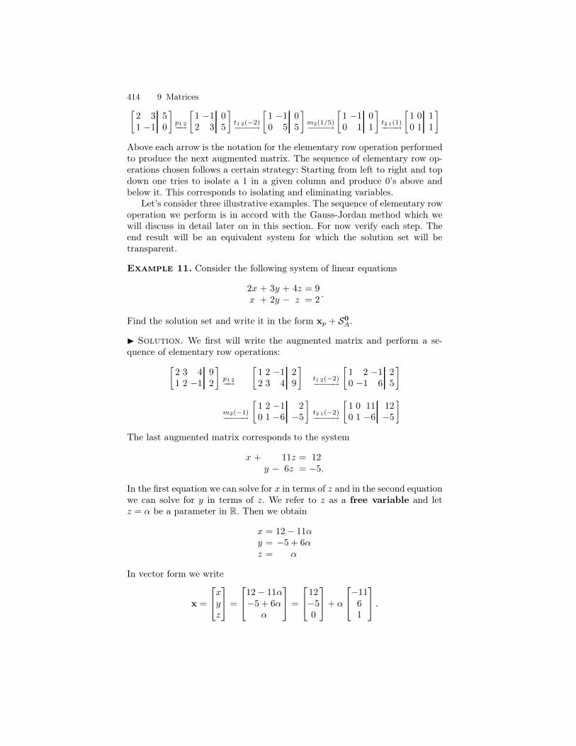
414 9 Matrices[
2 3 51 −1 0
]
p1 2−−→
[
1 −1 02 3 5
]
t1 2(−2)−−−−−→
[
1 −1 00 5 5
]
m2(1/5)−−−−−→
[
1 −1 00 1 1
]
t2 1(1)−−−−→
[
1 0 10 1 1
]
Above each arrow is the notation for the elementary row operation performedto produce the next augmented matrix. The sequence of elementary row op-erations chosen follows a certain strategy: Starting from left to right and topdown one tries to isolate a 1 in a given column and produce 0’s above andbelow it. This corresponds to isolating and eliminating variables.
Let’s consider three illustrative examples. The sequence of elementary rowoperation we perform is in accord with the Gauss-Jordan method which wewill discuss in detail later on in this section. For now verify each step. Theend result will be an equivalent system for which the solution set will betransparent.
Example 11. Consider the following system of linear equations
2x + 3y + 4z = 9x + 2y − z = 2
.
Find the solution set and write it in the form xp + S0A.
I Solution. We first will write the augmented matrix and perform a se-quence of elementary row operations:
[
2 3 4 91 2 −1 2
]
p1 2−−→
[
1 2 −1 22 3 4 9
]
t1 2(−2)−−−−−→
[
1 2 −1 20 −1 6 5
]
m2(−1)−−−−−→
[
1 2 −1 20 1 −6 −5
]
t2 1(−2)−−−−−→
[
1 0 11 120 1 −6 −5
]
The last augmented matrix corresponds to the system
x + 11z = 12y − 6z = −5.
In the first equation we can solve for x in terms of z and in the second equationwe can solve for y in terms of z. We refer to z as a free variable and letz = α be a parameter in R. Then we obtain
x = 12− 11αy = −5 + 6αz = α
In vector form we write
x =
xyz
=
12− 11α−5 + 6α
α
=
12−50
+ α
−1161
.
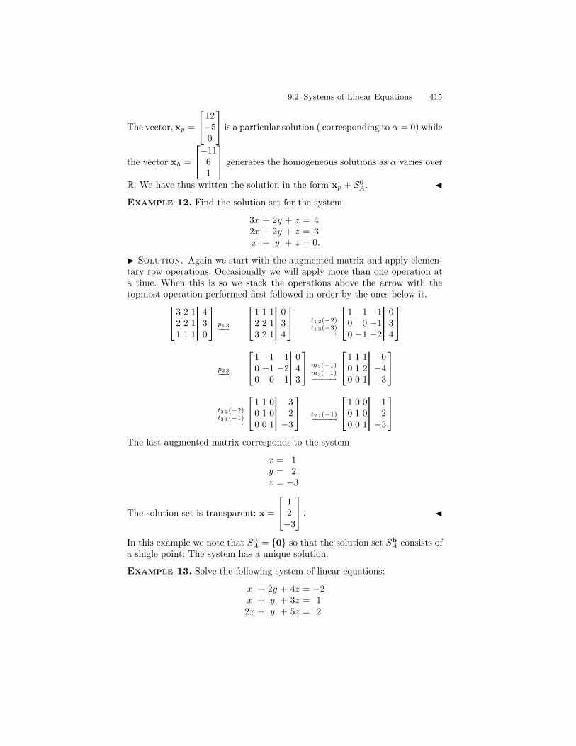
9.2 Systems of Linear Equations 415
The vector, xp =
12−50
is a particular solution ( corresponding to α = 0) while
the vector xh =
−1161
generates the homogeneous solutions as α varies over
R. We have thus written the solution in the form xp + S0A. J
Example 12. Find the solution set for the system
3x + 2y + z = 42x + 2y + z = 3x + y + z = 0.
I Solution. Again we start with the augmented matrix and apply elemen-tary row operations. Occasionally we will apply more than one operation ata time. When this is so we stack the operations above the arrow with thetopmost operation performed first followed in order by the ones below it.
3 2 1 42 2 1 31 1 1 0
p1 3−−→
1 1 1 02 2 1 33 2 1 4
t1 2(−2)t1 3(−3)−−−−−→
1 1 1 00 0 −1 30 −1 −2 4
p2 3−−→
1 1 1 00 −1 −2 40 0 −1 3
m2(−1)m3(−1)−−−−−→
1 1 1 00 1 2 −40 0 1 −3
t3 2(−2)t3 1(−1)−−−−−→
1 1 0 30 1 0 20 0 1 −3
t2 1(−1)−−−−−→
1 0 0 10 1 0 20 0 1 −3
The last augmented matrix corresponds to the system
x = 1y = 2z = −3.
The solution set is transparent: x =
12−3
. J
In this example we note that S0A = 0 so that the solution set Sb
A consists ofa single point: The system has a unique solution.
Example 13. Solve the following system of linear equations:
x + 2y + 4z = −2x + y + 3z = 12x + y + 5z = 2
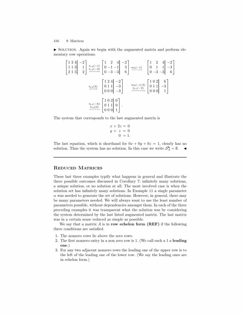
416 9 Matrices
I Solution. Again we begin with the augmented matrix and perform ele-mentary row operations.
1 2 4 −21 1 3 12 1 5 2
t1 2(−1)t1 3(−2)−−−−−→
1 2 4 −20 −1 −1 30 −3 −3 6
m2(−1)−−−−−→
1 2 4 −20 1 1 −30 −3 −3 6
t2 3(3)−−−−→
1 2 4 −20 1 1 −30 0 0 −3
m3(−1/3)t2 1(−2)
−−−−−−−→
1 0 2 60 1 1 −30 0 0 1
t3 1(−6)t3 2(3)−−−−−→
1 0 2 00 1 1 00 0 0 1
.
The system that corresponds to the last augmented matrix is
x + 2z = 0y + z = 0
0 = 1.
The last equation, which is shorthand for 0x + 0y + 0z = 1, clearly has nosolution. Thus the system has no solution. In this case we write Sb
A = ∅. J
Reduced Matrices
These last three examples typify what happens in general and illustrate thethree possible outcomes discussed in Corollary 7: infinitely many solutions,a unique solution, or no solution at all. The most involved case is when thesolution set has infinitely many solutions. In Example 11 a single parameterα was needed to generate the set of solutions. However, in general, there maybe many parameters needed. We will always want to use the least number ofparameters possible, without dependencies amongst them. In each of the threepreceding examples it was transparent what the solution was by consideringthe system determined by the last listed augmented matrix. The last matrixwas in a certain sense reduced as simple as possible.
We say that a matrix A is in row echelon form (REF) if the followingthree conditions are satisfied.
1. The nonzero rows lie above the zero rows.2. The first nonzero entry in a non zero row is 1. (We call such a 1 a leading
one.)3. For any two adjacent nonzero rows the leading one of the upper row is to
the left of the leading one of the lower row. (We say the leading ones arein echelon form.)
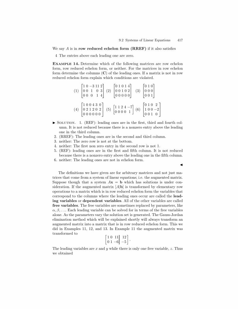
9.2 Systems of Linear Equations 417
We say A is in row reduced echelon form (RREF) if it also satisfies
4 The entries above each leading one are zero.
Example 14. Determine which of the following matrices are row echelonform, row reduced echelon form, or neither. For the matrices in row echelonform determine the columns (C) of the leading ones. If a matrix is not in rowreduced echelon form explain which conditions are violated.
(1)
1 0 −3 11 20 0 1 0 30 0 0 1 4
(2)
0 1 0 1 40 0 1 0 20 0 0 0 0
(3)
0 1 00 0 00 0 1
(4)
1 0 0 4 3 00 2 1 2 0 20 0 0 0 0 0
(5)
[
1 1 2 4 −70 0 0 0 1
]
(6)
0 1 0 21 0 0 −20 0 1 0
I Solution. 1. (REF): leading ones are in the first, third and fourth col-umn. It is not reduced because there is a nonzero entry above the leadingone in the third column.
2. (RREF): The leading ones are in the second and third column.3. neither: The zero row is not at the bottom.4. neither: The first non zero entry in the second row is not 1.5. (REF): leading ones are in the first and fifth column. It is not reduced
because there is a nonzero entry above the leading one in the fifth column.6. neither: The leading ones are not in echelon form.
J
The definitions we have given are for arbitrary matrices and not just ma-trices that come from a system of linear equations; i.e. the augmented matrix.Suppose though that a system Ax = b which has solutions is under con-sideration. If the augmented matrix [A|b] is transformed by elementary rowoperations to a matrix which is in row reduced echelon form the variables thatcorrespond to the columns where the leading ones occur are called the lead-ing variables or dependent variables. All of the other variables are calledfree variables. The free variables are sometimes replaced by parameters, likeα, β, . . .. Each leading variable can be solved for in terms of the free variablesalone. As the parameters vary the solution set is generated. The Gauss-Jordanelimination method which will be explained shortly will always transform anaugmented matrix into a matrix that is in row reduced echelon form. This wedid in Examples 11, 12, and 13. In Example 11 the augmented matrix wastransformed to
[
1 0 11 120 1 −6 −5
]
.
The leading variables are x and y while there is only one free variable, z. Thuswe obtained
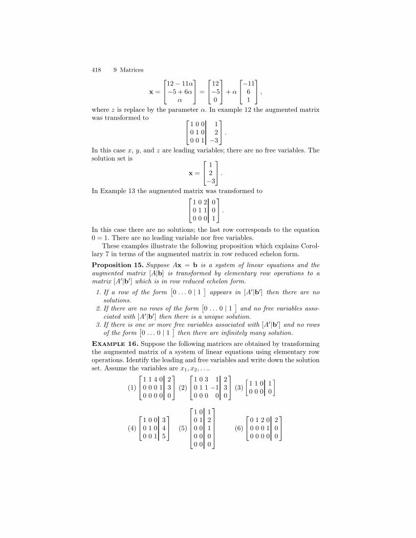
418 9 Matrices
x =
12− 11α−5 + 6α
α
=
12−50
+ α
−1161
,
where z is replace by the parameter α. In example 12 the augmented matrixwas transformed to
1 0 0 10 1 0 20 0 1 −3
.
In this case x, y, and z are leading variables; there are no free variables. Thesolution set is
x =
12−3
.
In Example 13 the augmented matrix was transformed to
1 0 2 00 1 1 00 0 0 1
.
In this case there are no solutions; the last row corresponds to the equation0 = 1. There are no leading variable nor free variables.
These examples illustrate the following proposition which explains Corol-lary 7 in terms of the augmented matrix in row reduced echelon form.
Proposition 15. Suppose Ax = b is a system of linear equations and theaugmented matrix [A|b] is transformed by elementary row operations to amatrix [A′|b′] which is in row reduced echelon form.
1. If a row of the form[
0 . . . 0 | 1]
appears in [A′|b′] then there are nosolutions.
2. If there are no rows of the form[
0 . . . 0 | 1]
and no free variables asso-ciated with [A′|b′] then there is a unique solution.
3. If there is one or more free variables associated with [A′|b′] and no rowsof the form
[
0 . . . 0 | 1]
then there are infinitely many solution.
Example 16. Suppose the following matrices are obtained by transformingthe augmented matrix of a system of linear equations using elementary rowoperations. Identify the leading and free variables and write down the solutionset. Assume the variables are x1, x2, . . ..
(1)
1 1 4 0 20 0 0 1 30 0 0 0 0
(2)
1 0 3 1 20 1 1 −1 30 0 0 0 0
(3)
[
1 1 0 10 0 0 0
]
(4)
1 0 0 30 1 0 40 0 1 5
(5)
1 0 10 1 20 0 10 0 00 0 0
(6)
0 1 2 0 20 0 0 1 00 0 0 0 0
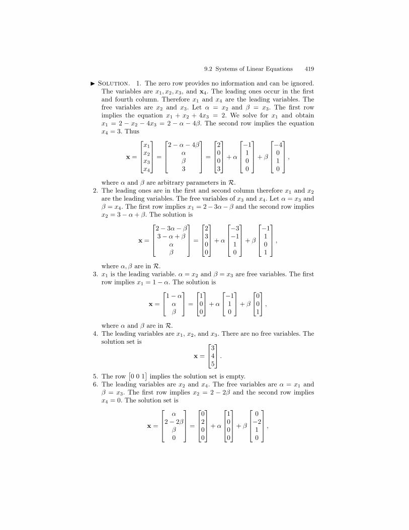
9.2 Systems of Linear Equations 419
I Solution. 1. The zero row provides no information and can be ignored.The variables are x1, x2, x3, and x4. The leading ones occur in the firstand fourth column. Therefore x1 and x4 are the leading variables. Thefree variables are x2 and x3. Let α = x2 and β = x3. The first rowimplies the equation x1 + x2 + 4x3 = 2. We solve for x1 and obtainx1 = 2 − x2 − 4x3 = 2 − α − 4β. The second row implies the equationx4 = 3. Thus
x =
x1
x2
x3
x4
=
2− α− 4βαβ3
=
2003
+ α
−1100
+ β
−4010
,
where α and β are arbitrary parameters in R.2. The leading ones are in the first and second column therefore x1 and x2
are the leading variables. The free variables of x3 and x4. Let α = x3 andβ = x4. The first row implies x1 = 2− 3α− β and the second row impliesx2 = 3− α+ β. The solution is
x =
2− 3α− β3− α+ β
αβ
=
2300
+ α
−3−110
+ β
−1101
,
where α, β are in R.3. x1 is the leading variable. α = x2 and β = x3 are free variables. The first
row implies x1 = 1− α. The solution is
x =
1− ααβ
=
100
+ α
−110
+ β
001
,
where α and β are in R.4. The leading variables are x1, x2, and x3. There are no free variables. The
solution set is
x =
345
.
5. The row[
0 0 1]
implies the solution set is empty.6. The leading variables are x2 and x4. The free variables are α = x1 andβ = x3. The first row implies x2 = 2 − 2β and the second row impliesx4 = 0. The solution set is
x =
α2− 2ββ0
=
0200
+ α
1000
+ β
0−210
,
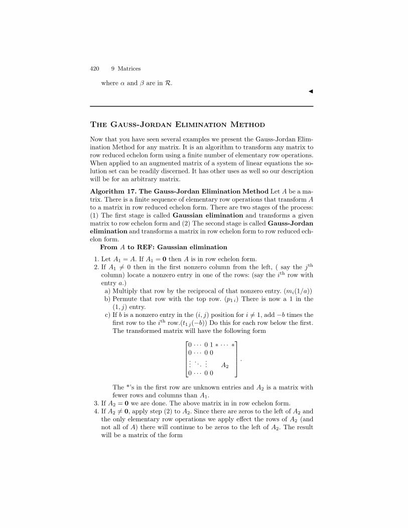
420 9 Matrices
where α and β are in R.J
The Gauss-Jordan Elimination Method
Now that you have seen several examples we present the Gauss-Jordan Elim-ination Method for any matrix. It is an algorithm to transform any matrix torow reduced echelon form using a finite number of elementary row operations.When applied to an augmented matrix of a system of linear equations the so-lution set can be readily discerned. It has other uses as well so our descriptionwill be for an arbitrary matrix.
Algorithm 17. The Gauss-Jordan Elimination Method Let A be a ma-trix. There is a finite sequence of elementary row operations that transform Ato a matrix in row reduced echelon form. There are two stages of the process:(1) The first stage is called Gaussian elimination and transforms a givenmatrix to row echelon form and (2) The second stage is called Gauss-Jordanelimination and transforms a matrix in row echelon form to row reduced ech-elon form.
From A to REF: Gaussian elimination
1. Let A1 = A. If A1 = 0 then A is in row echelon form.2. If A1 6= 0 then in the first nonzero column from the left, ( say the jth
column) locate a nonzero entry in one of the rows: (say the ith row withentry a.)a) Multiply that row by the reciprocal of that nonzero entry. (mi(1/a))b) Permute that row with the top row. (p1 i) There is now a 1 in the
(1, j) entry.c) If b is a nonzero entry in the (i, j) position for i 6= 1, add −b times the
first row to the ith row.(t1 j(−b)) Do this for each row below the first.The transformed matrix will have the following form
0 · · · 0 1 ∗ · · · ∗0 · · · 0 0...
. . .... A2
0 · · · 0 0
.
The *’s in the first row are unknown entries and A2 is a matrix withfewer rows and columns than A1.
3. If A2 = 0 we are done. The above matrix in in row echelon form.4. If A2 6= 0, apply step (2) to A2. Since there are zeros to the left of A2 and
the only elementary row operations we apply effect the rows of A2 (andnot all of A) there will continue to be zeros to the left of A2. The resultwill be a matrix of the form
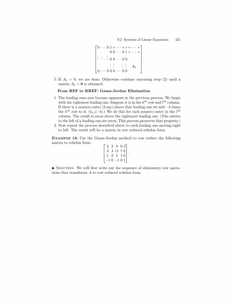
9.2 Systems of Linear Equations 421
0 · · · 0 1 ∗ · · · ∗ ∗ ∗ · · · ∗0 0 · · · 0 1 ∗ · · · ∗
.... . .
... 0 0 · · · 0 0...
......
... A3
0 · · · 0 0 0 · · · 0 0
.
5. If A3 = 0, we are done. Otherwise continue repeating step (2) until amatrix Ak = 0 is obtained.
From REF to RREF: Gauss-Jordan Elimination
1. The leading ones now become apparent in the previous process. We beginwith the rightmost leading one. Suppose it is in the kth row and lth column.If there is a nonzero entry (b say) above that leading one we add −b timesthe kth row to it. (tk j(−b).) We do this for each nonzero entry in the lth
column. The result is zeros above the rightmost leading one. (The entriesto the left of a leading one are zeros. This process preserves that property.)
2. Now repeat the process described above to each leading one moving rightto left. The result will be a matrix in row reduced echelon form.
Example 18. Use the Gauss-Jordan method to row reduce the followingmatrix to echelon form:
2 3 8 0 43 4 11 1 81 2 5 1 6−1 0 −1 0 1
.
I Solution. We will first write out the sequence of elementary row opera-tions that transforms A to row reduced echelon form.
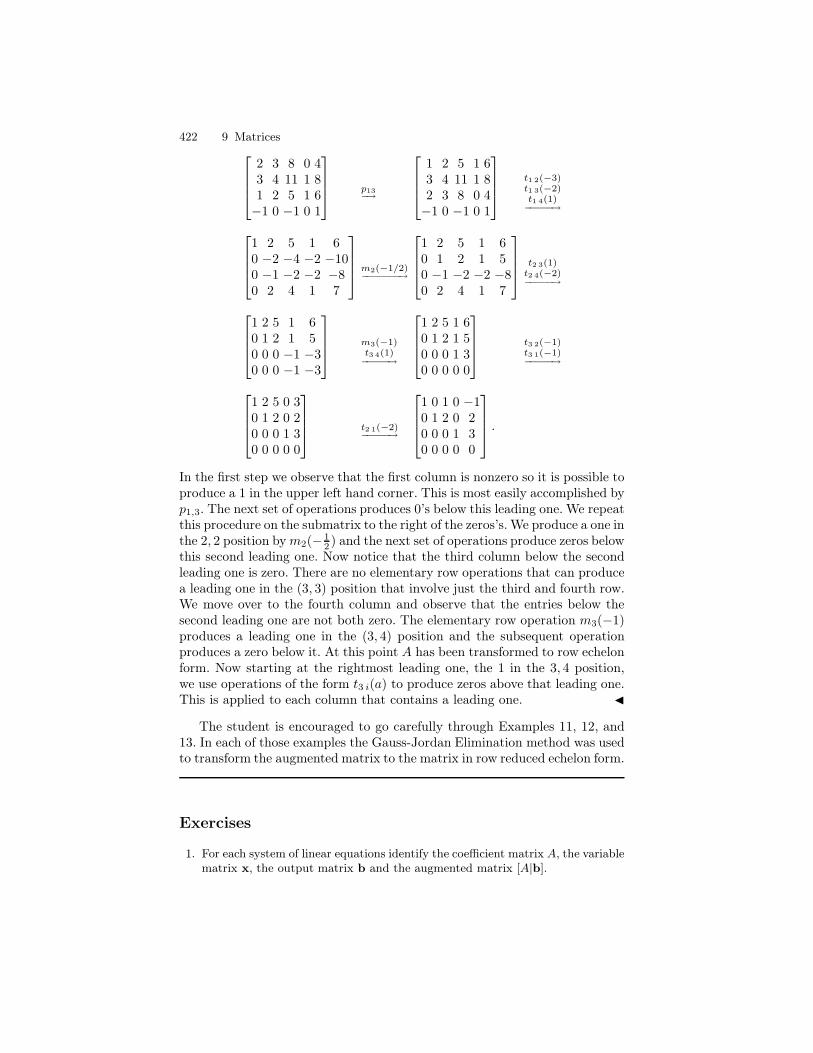
422 9 Matrices
2 3 8 0 43 4 11 1 81 2 5 1 6−1 0 −1 0 1
p13−→
1 2 5 1 63 4 11 1 82 3 8 0 4−1 0 −1 0 1
t1 2(−3)t1 3(−2)t1 4(1)−−−−−→
1 2 5 1 60 −2 −4 −2 −100 −1 −2 −2 −80 2 4 1 7
m2(−1/2)−−−−−−−→
1 2 5 1 60 1 2 1 50 −1 −2 −2 −80 2 4 1 7
t2 3(1)t2 4(−2)−−−−−→
1 2 5 1 60 1 2 1 50 0 0 −1 −30 0 0 −1 −3
m3(−1)t3 4(1)−−−−−→
1 2 5 1 60 1 2 1 50 0 0 1 30 0 0 0 0
t3 2(−1)t3 1(−1)−−−−−→
1 2 5 0 30 1 2 0 20 0 0 1 30 0 0 0 0
t2 1(−2)−−−−−→
1 0 1 0 −10 1 2 0 20 0 0 1 30 0 0 0 0
.
In the first step we observe that the first column is nonzero so it is possible toproduce a 1 in the upper left hand corner. This is most easily accomplished byp1,3. The next set of operations produces 0’s below this leading one. We repeatthis procedure on the submatrix to the right of the zeros’s. We produce a one inthe 2, 2 position bym2(− 1
2 ) and the next set of operations produce zeros belowthis second leading one. Now notice that the third column below the secondleading one is zero. There are no elementary row operations that can producea leading one in the (3, 3) position that involve just the third and fourth row.We move over to the fourth column and observe that the entries below thesecond leading one are not both zero. The elementary row operation m3(−1)produces a leading one in the (3, 4) position and the subsequent operationproduces a zero below it. At this point A has been transformed to row echelonform. Now starting at the rightmost leading one, the 1 in the 3, 4 position,we use operations of the form t3 i(a) to produce zeros above that leading one.This is applied to each column that contains a leading one. J
The student is encouraged to go carefully through Examples 11, 12, and13. In each of those examples the Gauss-Jordan Elimination method was usedto transform the augmented matrix to the matrix in row reduced echelon form.
Exercises
1. For each system of linear equations identify the coefficient matrix A, the variablematrix x, the output matrix b and the augmented matrix [A|b].
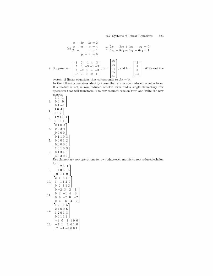
9.2 Systems of Linear Equations 423
(a)
x + 4y + 3z = 2x + y − z = 42x + z = 1
y − z = 6
(b)2x1 − 3x2 + 4x3 + x4 = 03x1 + 8x2 − 3x3 − 6x4 = 1
2. Suppose A =1 0 −1 4 3
5 3 −3 −1 −33 −2 8 4 −3−8 2 0 2 1
, x =x1
x2
x3
x4
x5
, and b = 2
13
−4 . Write out the
system of linear equations that corresponds to Ax = b.In the following matrices identify those that are in row reduced echelon form.If a matrix is not in row reduced echelon form find a single elementary rowoperation that will transform it to row reduced echelon form and write the newmatrix.
3. 1 0 10 0 00 1 −4
4. 1 0 40 1 2
5. 1 2 1 0 10 1 3 1 1
6. 0 1 0 30 0 2 60 0 0 0
7. 0 1 1 0 30 0 0 1 20 0 0 0 0
8. 1 0 1 0 30 1 3 4 13 0 3 0 9
Use elementary row operations to row reduce each matrix to row reduced echelonform.
9. 1 2 3 1−1 0 3 −50 1 1 0
10. 2 1 3 1 01 −1 1 2 00 2 1 1 2
11.0 −2 3 2 10 2 −1 4 00 6 −7 0 −20 4 −6 −4 −2
12.
1 2 1 1 52 4 0 0 61 2 0 1 30 0 1 1 2
13. −1 0 1 1 0 0
−3 1 3 0 1 07 −1 −4 0 0 1
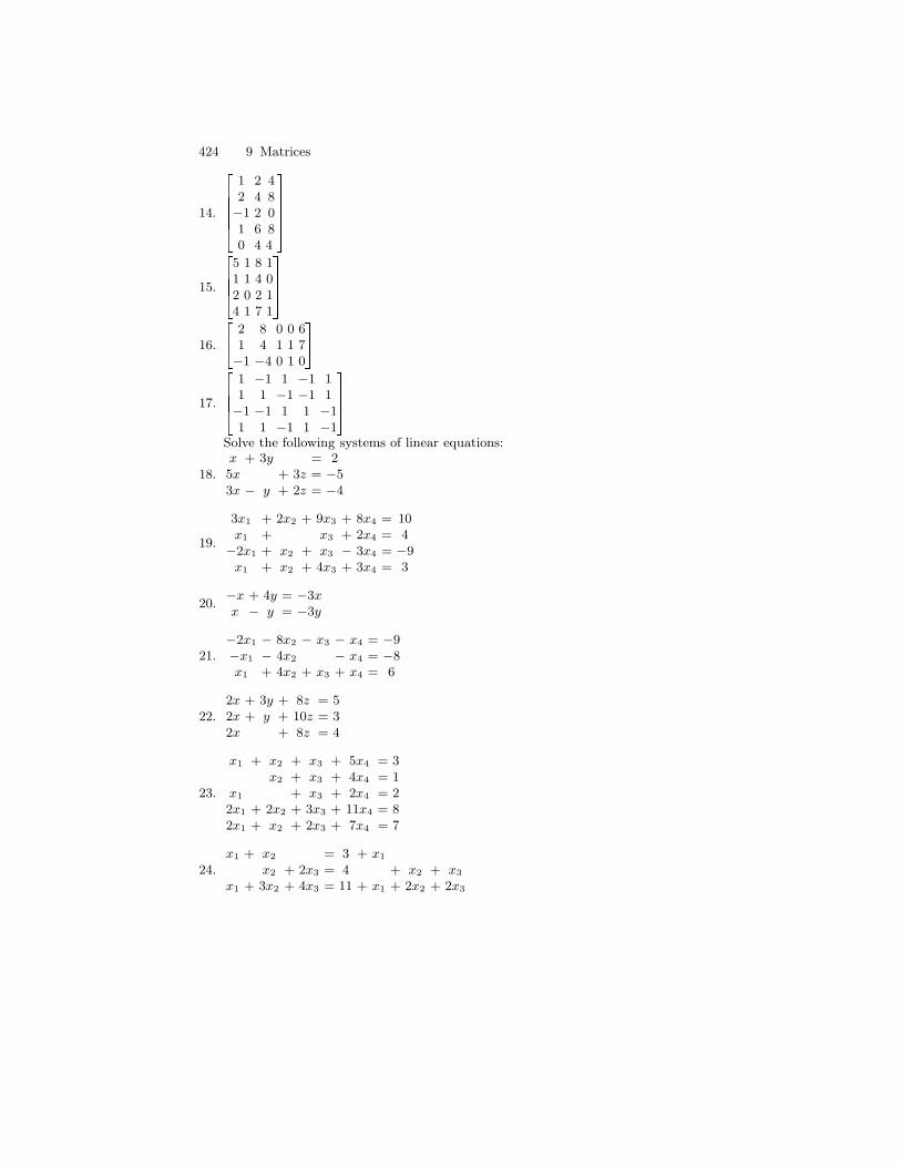
424 9 Matrices
14.
1 2 42 4 8−1 2 01 6 80 4 4
15.
5 1 8 11 1 4 02 0 2 14 1 7 1
16. 2 8 0 0 6
1 4 1 1 7−1 −4 0 1 0
17.1 −1 1 −1 1
1 1 −1 −1 1−1 −1 1 1 −11 1 −1 1 −1
Solve the following systems of linear equations:
18.x + 3y = 25x + 3z = −53x − y + 2z = −4
19.
3x1 + 2x2 + 9x3 + 8x4 = 10x1 + x3 + 2x4 = 4
−2x1 + x2 + x3 − 3x4 = −9x1 + x2 + 4x3 + 3x4 = 3
20.−x + 4y = −3xx − y = −3y
21.−2x1 − 8x2 − x3 − x4 = −9−x1 − 4x2 − x4 = −8x1 + 4x2 + x3 + x4 = 6
22.2x + 3y + 8z = 52x + y + 10z = 32x + 8z = 4
23.
x1 + x2 + x3 + 5x4 = 3x2 + x3 + 4x4 = 1
x1 + x3 + 2x4 = 22x1 + 2x2 + 3x3 + 11x4 = 82x1 + x2 + 2x3 + 7x4 = 7
24.x1 + x2 = 3 + x1
x2 + 2x3 = 4 + x2 + x3
x1 + 3x2 + 4x3 = 11 + x1 + 2x2 + 2x3
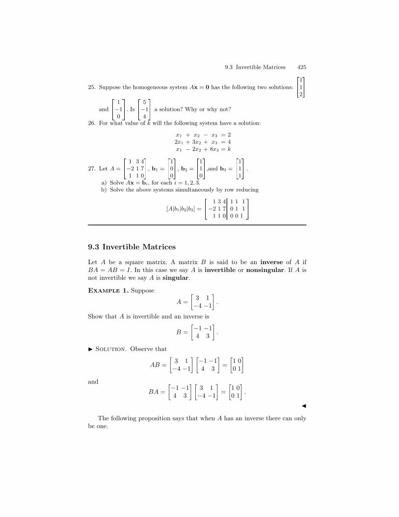
9.3 Invertible Matrices 425
25. Suppose the homogeneous system Ax = 0 has the following two solutions: 112
and 1−10 . Is 5
−14 a solution? Why or why not?
26. For what value of k will the following system have a solution:
x1 + x2 − x3 = 22x1 + 3x2 + x3 = 4x1 − 2x2 + 8x3 = k
27. Let A = 1 3 4−2 1 71 1 0, b1 = 10
0, b2 = 110,and b3 = 11
1 .
a) Solve Ax = bi, for each i = 1, 2, 3.b) Solve the above systems simultaneously by row reducing
[A|b1|b2|b3] = 1 3 4 1 1 1−2 1 7 0 1 1
1 1 0 0 0 1 9.3 Invertible Matrices
Let A be a square matrix. A matrix B is said to be an inverse of A ifBA = AB = I. In this case we say A is invertible or nonsingular. If A isnot invertible we say A is singular.
Example 1. Suppose
A =
[
3 1−4 −1
]
.
Show that A is invertible and an inverse is
B =
[
−1 −14 3
]
.
I Solution. Observe that
AB =
[
3 1−4 −1
] [
−1 −14 3
]
=
[
1 00 1
]
and
BA =
[
−1 −14 3
] [
3 1−4 −1
]
=
[
1 00 1
]
.
J
The following proposition says that when A has an inverse there can onlybe one.
426 9 Matrices
Proposition 2. Let A be an invertible matrix. Then the inverse is unique.
Proof. Suppose B and C are inverses of A. Then
B = BI = B(AC) = (BA)C = IC = C.
utBecause of uniqueness we can properly say the inverse of A when A is
invertible. In Example 1, the matrix B =
(
−1 −14 3
)
is the inverse of A; there
are no others. It is standard convention to denote the inverse of A by A−1.For many matrices it is possible to determine their inverse by inspection.
For example, the identity matrix In is invertible and its inverse is In: InIn =In. A diagonal matrix diag(a1, . . . , an) is invertible if each ai 6= 0, i = 1, . . . , n.The inverse then is simply diag( 1
a1, . . . , 1
an). However, if one of the ai is zero
then the matrix in not invertible. Even more is true. If A has a zero row, saythe ith row, then A is not invertible. To see this we get from Equation (2) inSection 9.1 that Rowi(AB) = Rowi(A)B = 0. Hence, there is no matrix B forwhich AB = I. Similarly, a matrix with a zero column cannot be invertible.
Proposition 3. Let A and B be invertible matrices. Then
1. A−1 is invertible and (A−1)−1 = A.2. AB is invertible and (AB)−1 = B−1A−1.
Proof. Suppose A and B are invertible. The symmetry of the equationA−1A = AA−1 = I says that A−1 is invertible and (A−1)−1 = A. Also(B−1A−1)(AB) = B−1(A−1A)B = B−1IB = B−1B = I and (AB)(B−1A−1) =A(B−1B)A−1 = AA−1 = I. This shows (AB)−1 = B−1A−1. ut
The following corollary easily follows:
Corollary 4. If A = A1 · · ·Ak is the product of invertible matrices then A isinvertible and A−1 = A−1
k · · ·A−11 .
Inversion Computations
Let ei be the column vector with 1 in the ith position and 0’s elsewhere. ByEquation (1) of Section 9.1 the equation AB = I implies that AColi(B) =Coli(I) = ei. This means that the solution to Ax = ei is the ith column ofthe inverse of A, when A is invertible. We can thus compute the inverse ofA one column at a time using the Gauss-Jordan elimination method on theaugmented matrix [A|ei]. Better yet, though, is to perform the Gauss-Jordanelimination method on the matrix [A|I]. If A is invertible it will reduce to amatrix of the form [I|B] and B will be A−1. If A is not invertible it will notbe possible to produce the identity in the first slot.
We illustrate this in the following two examples.
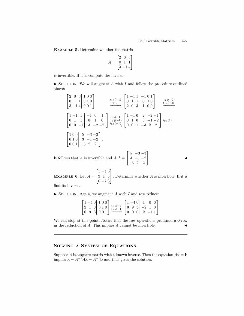
9.3 Invertible Matrices 427
Example 5. Determine whether the matrix
A =
2 0 30 1 13 −1 4
is invertible. If it is compute the inverse.
I Solution. We will augment A with I and follow the procedure outlinedabove:
2 0 3 1 0 00 1 1 0 1 03 −1 4 0 0 1
t1 3(−1)p1 3−−−−→
1 −1 1 −1 0 10 1 1 0 1 02 0 3 1 0 0
t1 3(−2)t2 3(−2)−−−−→
1 −1 1 −1 0 10 1 1 0 1 00 0 −1 3 −2 −2
m3(−1)t3 2(−1)t3 1(−1)−−−−→
1 −1 0 2 −2 −10 1 0 3 −1 −20 0 1 −3 2 2
t2 1(1)−−−→
1 0 0 5 −3 −30 1 0 3 −1 −20 0 1 −3 2 2
.
It follows that A is invertible and A−1 =
5 −3 −33 −1 −2−3 2 2
. J
Example 6. Let A =
1 −4 02 1 30 −7 3
. Determine whether A is invertible. If it is
find its inverse.
I Solution. Again, we augment A with I and row reduce:
1 −4 0 1 0 02 1 3 0 1 00 9 3 0 0 1
t1 2(−2)t2 3(−1)−−−−→
1 −4 0 1 0 00 9 3 −2 1 00 0 0 2 −1 1
We can stop at this point. Notice that the row operations produced a 0 rowin the reduction of A. This implies A cannot be invertible. J
Solving a System of Equations
Suppose A is a square matrix with a known inverse. Then the equation Ax = b
implies x = A−1Ax = A−1b and thus gives the solution.
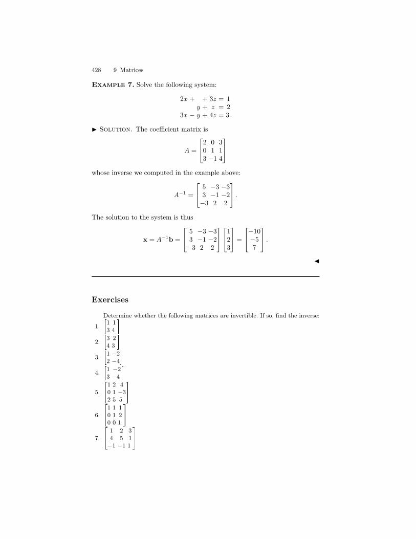
428 9 Matrices
Example 7. Solve the following system:
2x + + 3z = 1y + z = 2
3x − y + 4z = 3.
I Solution. The coefficient matrix is
A =
2 0 30 1 13 −1 4
whose inverse we computed in the example above:
A−1 =
5 −3 −33 −1 −2−3 2 2
.
The solution to the system is thus
x = A−1b =
5 −3 −33 −1 −2−3 2 2
123
=
−10−57
.
J
Exercises
Determine whether the following matrices are invertible. If so, find the inverse:
1. 1 13 4
2. 3 24 3
3. 1 −22 −4
4. 1 −23 −4
5. 1 2 40 1 −32 5 5
6. 1 1 10 1 20 0 1
7. 1 2 34 5 1−1 −1 1
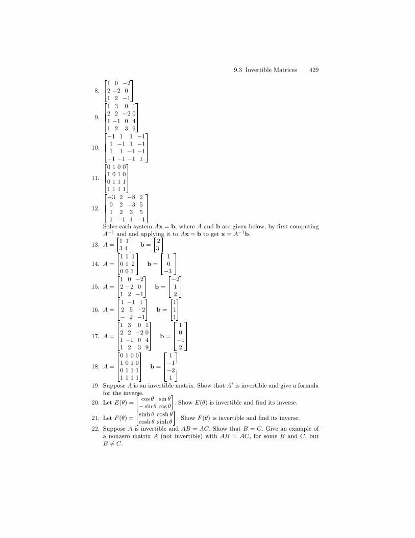
9.3 Invertible Matrices 429
8. 1 0 −22 −2 01 2 −1
9.1 3 0 12 2 −2 01 −1 0 41 2 3 9
10.
−1 1 1 −11 −1 1 −11 1 −1 −1−1 −1 −1 1
11.
0 1 0 01 0 1 00 1 1 11 1 1 1
12.
−3 2 −8 20 2 −3 51 2 3 51 −1 1 −1
Solve each system Ax = b, where A and b are given below, by first computingA−1 and and applying it to Ax = b to get x = A−1b.
13. A = 1 13 4 b = 23
14. A = 1 1 10 1 20 0 1 b = 1
0−3
15. A = 1 0 −22 −2 01 2 −1 b = −2
12
16. A = 1 −1 12 5 −2− 2 −1 b = 11
117. A =
1 3 0 12 2 −2 01 −1 0 41 2 3 9
b =1
0−12
18. A =
0 1 0 01 0 1 00 1 1 11 1 1 1
b =1−1−21
19. Suppose A is an invertible matrix. Show that At is invertible and give a formula
for the inverse.
20. Let E(θ) = cos θ sin θ− sin θ cos θ. Show E(θ) is invertible and find its inverse.
21. Let F (θ) = sinh θ cosh θcosh θ sinh θ . Show F (θ) is invertible and find its inverse.
22. Suppose A is invertible and AB = AC. Show that B = C. Give an example ofa nonzero matrix A (not invertible) with AB = AC, for some B and C, butB 6= C.
430 9 Matrices
9.4 Determinants
In this section we will discuss the definition of the determinant and someof its properties. For our purposes the determinant is a very useful numberthat we can associate to a square matrix. The determinant has an wide rangeof applications. It can be used to determine whether a matrix is invertible.Cramer’s rule gives the unique solution to a system of linear equations asthe quotient of determinants. In multidimensional calculus, the Jacobian isgiven by a determinant and expresses how area or volume changes under atransformation. Most students by now are familiar with the definition of the
determinant for a 2 × 2 matrix: Let A =
[
a bc d
]
. The determinant of A is
given bydet(A) = ad− bc.
It is the product of the diagonal entries minus the product of the off diagonal
entries. For example, det
[
1 35 −2
]
= 1 · (−2)− 5 · 3 = −17.
The definition of the determinant for an n × n matrix is decidedly morecomplicated. We will present an inductive definition. Let A be an n×n matrixand let A(i, j) be the matrix obtained from A by deleting the ith row and jth
column. Since A(i, j) is an (n− 1)× (n− 1) matrix we can inductively definethe (i, j) minor, Minori j(A), to be the determinant of A(i, j):
Minori j(A) = det(A(i, j)).
The following theorem, whose proof is extremely tedious and we omit, isthe basis for the definition of the determinant.
Theorem 1 (Laplace expansion formulas). Suppose A is an n× n ma-trix. Then the following numbers are all equal and we call this number thedeterminant of A:
detA =
n∑
j=1
(−1)i+jai,jMinori j(A) for each i
and
detA =
n∑
i=1
(−1)i+jai,jMinori j(A) for each j.
Any of these formulas can thus be taken as the definition of the determi-nant. In the first formula the index i is fixed and the sum is taken over all j.The entries ai,j thus fill out the ith row. We therefore call this formula theLaplace expansion of the determinant along the ith row or simply a
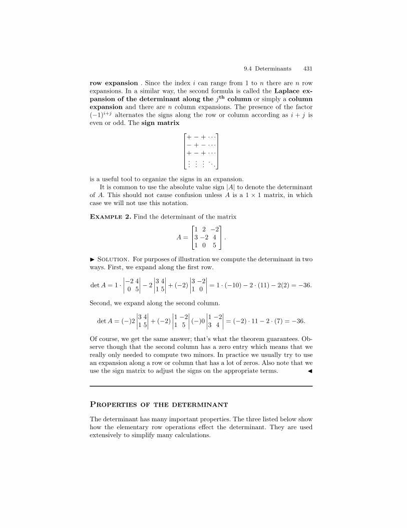
9.4 Determinants 431
row expansion . Since the index i can range from 1 to n there are n rowexpansions. In a similar way, the second formula is called the Laplace ex-pansion of the determinant along the jth column or simply a columnexpansion and there are n column expansions. The presence of the factor(−1)i+j alternates the signs along the row or column according as i + j iseven or odd. The sign matrix
+ − + · · ·− + − · · ·+ − + · · ·...
......
. . .
is a useful tool to organize the signs in an expansion.It is common to use the absolute value sign |A| to denote the determinant
of A. This should not cause confusion unless A is a 1 × 1 matrix, in whichcase we will not use this notation.
Example 2. Find the determinant of the matrix
A =
1 2 −23 −2 41 0 5
.
I Solution. For purposes of illustration we compute the determinant in twoways. First, we expand along the first row.
detA = 1 ·∣
∣
∣
∣
−2 40 5
∣
∣
∣
∣
− 2
∣
∣
∣
∣
3 41 5
∣
∣
∣
∣
+ (−2)
∣
∣
∣
∣
3 −21 0
∣
∣
∣
∣
= 1 · (−10)− 2 · (11)− 2(2) = −36.
Second, we expand along the second column.
detA = (−)2
∣
∣
∣
∣
3 41 5
∣
∣
∣
∣
+ (−2)
∣
∣
∣
∣
1 −21 5
∣
∣
∣
∣
(−)0
∣
∣
∣
∣
1 −23 4
∣
∣
∣
∣
= (−2) · 11− 2 · (7) = −36.
Of course, we get the same answer; that’s what the theorem guarantees. Ob-serve though that the second column has a zero entry which means that wereally only needed to compute two minors. In practice we usually try to usean expansion along a row or column that has a lot of zeros. Also note that weuse the sign matrix to adjust the signs on the appropriate terms. J
Properties of the determinant
The determinant has many important properties. The three listed below showhow the elementary row operations effect the determinant. They are usedextensively to simplify many calculations.
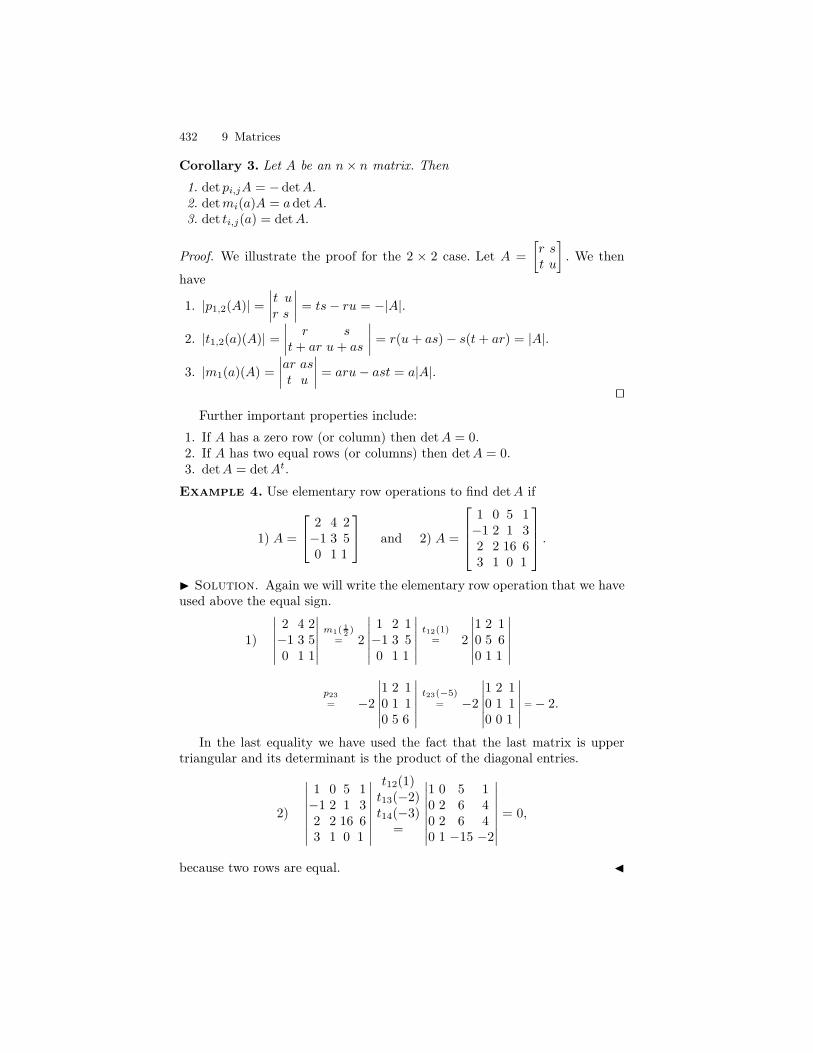
432 9 Matrices
Corollary 3. Let A be an n× n matrix. Then
1. det pi,jA = − detA.2. detmi(a)A = a detA.3. det ti,j(a) = detA.
Proof. We illustrate the proof for the 2 × 2 case. Let A =
[
r st u
]
. We then
have
1. |p1,2(A)| =∣
∣
∣
∣
t ur s
∣
∣
∣
∣
= ts− ru = −|A|.
2. |t1,2(a)(A)| =∣
∣
∣
∣
r st+ ar u+ as
∣
∣
∣
∣
= r(u + as)− s(t+ ar) = |A|.
3. |m1(a)(A) =
∣
∣
∣
∣
ar ast u
∣
∣
∣
∣
= aru− ast = a|A|.ut
Further important properties include:
1. If A has a zero row (or column) then detA = 0.2. If A has two equal rows (or columns) then detA = 0.3. detA = detAt.
Example 4. Use elementary row operations to find detA if
1) A =
2 4 2−1 3 50 1 1
and 2) A =
1 0 5 1−1 2 1 32 2 16 63 1 0 1
.
I Solution. Again we will write the elementary row operation that we haveused above the equal sign.
1)
∣
∣
∣
∣
∣
∣
2 4 2−1 3 50 1 1
∣
∣
∣
∣
∣
∣
m1(12 )
= 2
∣
∣
∣
∣
∣
∣
1 2 1−1 3 50 1 1
∣
∣
∣
∣
∣
∣
t12(1)= 2
∣
∣
∣
∣
∣
∣
1 2 10 5 60 1 1
∣
∣
∣
∣
∣
∣
p23
= −2
∣
∣
∣
∣
∣
∣
1 2 10 1 10 5 6
∣
∣
∣
∣
∣
∣
t23(−5)= −2
∣
∣
∣
∣
∣
∣
1 2 10 1 10 0 1
∣
∣
∣
∣
∣
∣
=− 2.
In the last equality we have used the fact that the last matrix is uppertriangular and its determinant is the product of the diagonal entries.
2)
∣
∣
∣
∣
∣
∣
∣
∣
1 0 5 1−1 2 1 32 2 16 63 1 0 1
∣
∣
∣
∣
∣
∣
∣
∣
t12(1)t13(−2)t14(−3)
=
∣
∣
∣
∣
∣
∣
∣
∣
1 0 5 10 2 6 40 2 6 40 1 −15 −2
∣
∣
∣
∣
∣
∣
∣
∣
= 0,
because two rows are equal. J
9.4 Determinants 433
In the following example we use elementary row operations to zero outentries in a column and then use a Laplace expansion formula.
Example 5. Find the determinant of
A =
1 4 2 −12 2 3 0−1 1 2 40 1 3 2
.
I Solution.
det(A) =
∣
∣
∣
∣
∣
∣
∣
∣
1 4 2 −12 2 3 0−1 1 2 40 1 3 2
∣
∣
∣
∣
∣
∣
∣
∣
t1,2(−2)t1,3(1)
=
∣
∣
∣
∣
∣
∣
∣
∣
1 4 2 −10 −6 −1 20 5 4 30 1 3 2
∣
∣
∣
∣
∣
∣
∣
∣
=
∣
∣
∣
∣
∣
∣
−6 −1 25 4 31 3 2
∣
∣
∣
∣
∣
∣
t3,1(6)t3,2(−5)
=
∣
∣
∣
∣
∣
∣
0 17 140 −11 −71 3 2
∣
∣
∣
∣
∣
∣
=
∣
∣
∣
∣
17 14−11 −7
∣
∣
∣
∣
= −119 + 154 = 35
J
The following theorem contains two very important properties of the de-terminant. We will omit the proof.
Theorem 6.1. A square matrix A is invertible if and only if detA 6= 0.2. If A and B are square matrices of the same size then
det(AB) = detAdetB.
The cofactor and adjoint matrices
Again, let A be a square matrix. We define the cofactor matrix, Cof(A), of Ato be the matrix whose (i, j)-entry is (−1)i+jMinori,j . We define the adjointmatrix, Adj(A), of A by the formula Adj(A) = (Cof(A))t. The important roleof the adjoint matrix is seen in the following theorem and its corollary.
Theorem 7. For A a square matrix we have
A Adj(A) = Adj(A) A = det(A)I.
434 9 Matrices
Proof. The (i, j) entry of A Adj(A) is
n∑
k=0
Ai k(Adj(A))k j =n∑
k=0
(−1)k+jAi kMinork j(A).
When i = j this is a Laplace expansion formula and is hence detA by Theorem1. When i 6= j this is the expansion of a determinant for a matrix with twoequal rows and hence is zero. ut
The following corollary immediately follows.
Corollary 8 (The adjoint inversion formula). If detA 6= 0 then
A−1 =1
detAAdj(A).
The inverse of a 2 × 2 matrix is a simple matter: Let A =
[
a bc d
]
. Then
Adj(A) =
[
d −b−c a
]
and if det(A) = ad− bd 6= 0 then
A−1 =1
ad− bc
[
d −b−c a
]
. (1)
For an example suppose A =
[
1 −3−2 1
]
. Then det(A) = 1 − (6) = −5 6= 0 so
A is invertible and A−1 = −15
[
1 32 1
]
=
[−15
−35
−25
−15
]
.
The general formula for the inverse of a 3 × 3 is substantially more com-plicated and difficult to remember. Consider though an example.
Example 9. Let
A =
1 2 01 4 1−1 0 3
.
Find its inverse if it is invertible.
I Solution. We expand along the first row to compute the determinant
and get det(A) = 1 det
[
4 10 3
]
− 2 det
[
1 1−1 3
]
= 1(12) − 2(4) = 4. Thus A
is invertible. The cofactor of A is Cof(A) =
12 −4 4−6 3 −22 −1 2
and Adj(A) =
Cof(A)t =
12 −6 2−4 3 −14 −2 2
. The inverse of A is thus
9.4 Determinants 435
A−1 =1
4
12 −6 2−4 3 −14 −2 2
=
3 −32
12
−1 34
−14
1 −12
12
.
J
In our next example we will consider a matrix with entries in R = R[s].Such matrices will arise naturally in Chapter 10.
Example 10. Let
A =
1 2 10 1 31 1 2
.
Find the inverse of the matrix
sI −A =
s− 1 −2 −10 s− 1 −3−1 −1 s− 2
.
I Solution. A straightforward computation gives det(sI−A) = (s−4)(s2+1). The matrix of minors for sI −A is
(s− 1)(s− 2)− 3 −3 s− 1−2(s− 2)− 1 (s− 1)(s− 2)− 1 −(s− 1)− 26 + (s− 1) −3(s− 1) (s− 1)2
.
After simplifying somewhat we obtain the cofactor matrix
s2 − 3s− 1 3 s− 12s− 3 s2 − 3s+ 1 s+ 1s+ 5 3s− 3 (s− 1)2
.
The adjoint matrix is
s2 − 3s− 1 2s− 3 s+ 53 s2 − 3s+ 1 3s− 3
s− 1 s+ 1 (s− 1)2
.
Finally, we obtain the inverse:
(sI −A)−1 =
s2−3s−1(s−4)(s2+1)
2s−3(s−4)(s2+1)
s+5(s−4)(s2+1)
3(s−4)(s2+1)
s2−3s+1(s−4)(s2+1)
3s−3(s−4)(s2+1)
s−1(s−4)(s2+1)
s+1(s−4)(s2+1)
(s−1)2
(s−4)(s2+1)
.
J
436 9 Matrices
Cramer’s Rule
We finally consider a well known theoretical tool used to solve a system Ax =b when A is invertible. Let A(i,b) denote the matrix obtained by replacingthe ith column of A with the column vector b. We then have the followingtheorem:
Theorem 11. Suppose detA 6= 0. Then the solution to Ax = b is givencoordinate wise by the formula:
xi =detA(i,b)
detA.
Proof. Since A is invertible we have
xi = (A−1b)i =
n∑
k=1
(A−1)i kbk
=1
detA
n∑
k=1
(−1)i+kMinork i(A)bk
=1
det(A)
n∑
k=1
(−1)i+kbkMinork i(A) =detA(i,b)
detA.
ut
The following example should convince you that Cramer’s Rule is mainlya theoretical tool and not a practical one for solving a system of linear equa-tions. The Gauss-Jordan elimination method is usually far more efficient thancomputing n+ 1 determinants for a system Ax = b, where A is n× n.
Example 12. Solve the following system of linear equations using Cramer’sRule.
x + y + z = 02x + 3y − z = 11x + z = −2
I Solution. We have
detA =
∣
∣
∣
∣
∣
∣
1 1 12 3 −11 0 1
∣
∣
∣
∣
∣
∣
= −3,
detA(1,b) =
∣
∣
∣
∣
∣
∣
0 1 111 3 −1−2 0 1
∣
∣
∣
∣
∣
∣
= −3,
9.4 Determinants 437
detA(2,b) =
∣
∣
∣
∣
∣
∣
1 0 12 11 −11 −2 1
∣
∣
∣
∣
∣
∣
= −6,
and detA(3,b) =
∣
∣
∣
∣
∣
∣
1 1 02 3 111 0 −2
∣
∣
∣
∣
∣
∣
= 9,
where b =
011−2
. Since detA 6= 0 Cramer’s Rule gives
x1 =detA(1,b)
detA=−3
−3= 1,
x2 =detA(2,b)
detA=−6
−3= 2,
and
x3 =detA(3,b)
detA=
9
−3= −3.
J
Exercises
Find the determinant of each matrix given below in three ways: a row expansion,a column expansion, and using row operations to reduce to a triangular matrix.
1. 1 42 9
2. 1 14 4
3. 3 42 6
4. 1 1 −11 4 02 3 1
5. 4 0 38 1 73 4 1
6. 3 98 1000 2 990 0 1
7.0 1 −2 4
2 3 9 21 4 8 3−2 3 −2 4
438 9 Matrices
8.−4 9 −4 1
2 3 0 −4−2 3 5 −6−3 2 0 1
9.
2 4 2 31 2 1 44 8 4 61 9 11 13
Find the inverse of (sI−A) and determine for which values of s det(sI−A) = 0.
10. 1 21 2
11. 3 11 3
12. 1 1−1 1
13. 1 0 10 1 00 3 1
14. 1 −3 3−3 1 33 −3 1
15. 0 4 0−1 0 01 4 −1
Use the adjoint formula for the inverse for the matrices given below.
16. 1 42 9
17. 1 14 4
18. 3 42 6
19. 1 1 −11 4 02 3 1
20. 4 0 38 1 73 4 1
21. 3 98 1000 2 990 0 1
22.0 1 −2 4
2 3 9 21 4 8 3−2 3 −2 4
23.
−4 9 −4 12 3 0 −4−2 3 5 −6−3 2 0 1
9.4 Determinants 439
24.2 4 2 31 2 1 44 8 4 61 9 11 13

10
Systems of Differential Equations
10.1 Systems of Differential Equations
10.1.1 Introduction
In the previous chapters we have discussed ordinary differential equations ina single unknown function. These are adequate to model real world systemsas they evolve in time, provided that only one state, i.e., one number y(t),is necessary to describe the system. For instance, we might be interested inthe way that the population of a species changes over time, the way thetemperature of an object changes over time, the way the concentration ofa pollutant in a lake changes over time, or the displacement over time of aweight attached to a spring. In each of these cases, the system we wish todescribe is adequately represented by a single number. In the examples listed,the number is the population p(t) at time t, the temperature T (t) at time t,the concentration c(t) of a pollutant at time t, or the displacement y(t) ofthe weight from equilibrium. However, a single ordinary differential equationis inadequate for describing the evolution over time of a system which needsmore than one number to describe its state at a given time t. For example,an ecological system consisting of two species will require two numbers p1(t)and p2(t) to describe the population of each species at time t, i.e., to describea system consisting of a population of rabbits and foxes, you need to givethe population of both rabbits and foxes at time t. Moreover, the descriptionof the way this system changes with time will involve the derivatives p′1(t),p′2(t), the functions p1(t), p2(t) themselves, and possibly the variable t. Thisis precisely what is intended by a system of ordinary differential equations.
A system of ordinary differential equations is a system of equationsrelating several unknown functions yi(t) of an independent variable t, someof the derivatives of the yi(t), and possibly t itself. As for a single differentialequation, the order of a system of differential equations is the highest orderderivative which appears in any equation.
442 10 Systems of Differential Equations
Example 1. The following two equations
y′1 = ay1 − by1y2y′2 = −cy1 + dy1y2
(1)
constitute a system of ordinary differential equations involving the unknownfunctions y1 and y2. Note that in this example the number of equations isequal to the number of unknown functions. This is the typical situation whichoccurs in practice.
Example 2. Suppose that a particle of mass m moves in a force fieldF = (F1, F2, F3) that depends on time t, the position of the particle x(t) =(x1(t), x2(t), x3(t)) and the velocity of the particle x′(t) = (x′1(t), x
′2(t), x
′3(t)).
Then Newton’s second law of motion states, in vector form, that F = ma,where a = x′′ is the acceleration. Writing out what this says in components,we get a system of second order differential equations
mx′′1 (t) = F1(t, x1(t), x2(t), x3(t), x′1(t), x
′2(t), x
′3(t))
mx′′2 (t) = F2(t, x1(t), x2(t), x3(t), x′1(t), x
′2(t), x
′3(t))
mx′′3 (t) = F3(t, x1(t), x2(t), x3(t), x′1(t), x
′2(t), x
′3(t)).
(2)
In this example, the state at time t is described by six numbers, namely thethree coordinates and the three velocities, and these are related by the threeequations described above. The resulting system of equations is a second ordersystem of differential equations since the equations include second order deriv-atives of some of the unknown functions. Notice that in this example we havesix states, namely the three coordinates of the position vector and the threecoordinates of the velocity vector, but only three equations. Nevertheless, itis easy to put this system in exactly the same theoretical framework as thefirst example by renaming the states as follows. Let y = (y1, y2, y3, y4, y5, y6)where y1 = x1, y2 = x2, y3 = x3, y4 = x′1, y5 = x′2, and y6 = x′3. Using thesenew function names, the system of equations (2) can be rewritten using onlyfirst derivatives:
y′1 = y4
y′2 = y5
y′3 = y6
y′4 =1
mF1(t, y1, y2, y3, y4, y5, y6)
y′5 =1
mF2(t, y1, y2, y3, y4, y5, y6)
y′6 =1
mF3(t, y1, y2, y3, y4, y5, y6).
(3)
Note that this can be expressed as a vector equation
y′ = f(t,y)
10.1 Systems of Differential Equations 443
where
f(t,y) = (y4, y5, y6,1
mF1(t,y),
1
mF2(t,y),
1
mF3(t,y)).
The trick used in Example 2 to reduce the second order system to a firstorder system in a larger number of variables works in general, so that it isonly really necessary to consider first order systems of differential equations.
As with a single first order ordinary differential equation, it is convenientto consider first order systems in a standard form for purposes of describingproperties and solution algorithms for these systems.
Definition 3. The standard form for a first order system of ordinary dif-ferential equations is a vector equation of the form
y′ = f(t,y) (4)
where f : U → Rn is a function from an open subset U of Rn+1 to Rn. If aninitial point t0 and an initial vector y0 are also specified, then one obtains aninitial value problem:
y′ = f(t,y), y(t0) = y0. (5)
A solution of Equation (4) is a differentiable vector function y : I → Rn
where I is an open interval in R and the function y satisfies Equation (4) forall t ∈ I. This means that
y′(t) = f(t,y(t)) (6)
for all t ∈ I. If also y(t0) = y0, then y(t) is a solution of the initial valueproblem (5).
Equation (1) is a system in standard form where n = 2. That is, thereare two unknown functions y1 and y2 which can be incorporated into a twodimensional vector y = (y1, y2), and if f(t,y) = (f1(t, y1, y2), f2(t, y1,2 )) =(ay1 − by1y2, −cy1 + dy1y2), then Equation (5) is a short way to write thesystem of equations
y′1 = ay1 − by1y2 = f1(t, y1, y2)y′2 = −cy1 + dy1y2 = f2(t, y1, y2).
(7)
Equation (3) of Example 2 is a first order system with n = 6. We shallprimarily concentrate on the study of systems where n = 2 or n = 3, butExample 2 shows that even very simple real world systems can lead to systemsof differential equations with a large number of unknown functions.
Example 4. Consider the following first order system of ordinary differen-tial equations:
y′1 = 3y1 − y2y′2 = 4y1 − 2y2.
(8)
444 10 Systems of Differential Equations
1. Verify that y(t) = (y1(t), y2(t)) = (e2t, e2t) is a solution of Equation (8).
I Solution. Since y1(t) = y2(t) = e2t,
y′1(t) = 2e2t = 3e2t − e2t = 3y1(t)− y2(t)and y′2(t) = 2e2t = 4e2t − 2e2t = 4y1(t)− 2y2(t),
which is precisely what it means for y(t) to satisfy (8). J
2. Verify that z(t) = (z1(t), z2(t)) = (e−t, 4e−t) is a solution of Equation(8).
I Solution. As above, we calculate
z′1(t) = −e−t = 3e−t − 4e−t = 3z1(t)− z2(t)and z′2(t) = −4e−t = 4e−t − 2 · 4e−t = 4z1(t)− 2z2(t),
which is precisely what it means for z(t) to satisfy (8). J
3. If c1 and c2 are any constants, verify that w(t) = c1y(t) + c2z(t) is alsoa solution of Equation (8).
I Solution. Note that w(t) = (w1(t), w2(t)), where w1(t) = c1y1(t) +c2z1(t) = c1e
2t + c2e−t and w2(t) = c1y2(t) + c2z2(t) = c1e
2t + c24e−t.
Then
w′1(t) = 2c1e
2t − c2e−t = 3w1(t)− w2(t)
and w′2(t) = 2c1e
−t − 4c2e−t = 4w1(t)− 2w2(t).
Again, this is precisely what it means for w(t) to be a solution of (8).We shall see in the next section that w(t) is, in fact, the general solutionof Equation (8). That is, any solution of this equation is obtained by aparticular choice of the constants c1 and c2. J
Example 5. Consider the following first order system of ordinary differen-tial equations:
y′1 = 3y1 − y2 + 2ty′2 = 4y1 − 2y2 + 2.
(9)
Notice that this is just Equation (8) with one additional term (not involvingthe unknown functions y1 and y2) added to each equation.
1. Verify that yp(t) = (yp1(t), yp2(t)) = (−2t + 1, −4t + 5) is a solution ofEquation (9).
I Solution. Since yp1(t) = −2t+ 1 and yp2(t) = −4t+ 5, direct calcu-lation gives y′p1(t) = −2, y′p2(t) = −4 and
3yp1(t)− yp2(t) + 2t = 3(−2t+ 1)− (−4t+ 5) + 2t = −2 = y′p1(t)
and 4y′p1(t)− 2y′p2(t) + 2 = 4(−2t+ 1)− 2(−4t+ 5) + 2 = −4 = y′p2(t).
Hence yp(t) is a solution of (9). J
10.1 Systems of Differential Equations 445
2. Verify that zp(t) = 2yp(t) = (zp1(t), zp2(t)) = (−4t+ 2, −8t+ 10) is nota solution to Equation (9).
I Solution. Since
3zp1(t)−zp2(t)+2t = 3(−4t+2)−(−8t+10)+2t= −2t−4 6= −4 = z′p1(t),
zp(t) fails to satisfy the first of the two equations of (9), and hence is nota solution of the system. J
3. We leave it as an exercise to verify that yg(t) = w(t)+yp(t) is a solution of(9), where w(t) is the general solution of Equation (8) from the previousexample.
We will now list some particular classes of first order systems of ordinarydifferential equations. As for the case of a single differential equation, it ismost convenient to identify these classes by describing properties of the righthand side of the equation when it is expressed in standard form.
Definition 6. The first order system in standard form
y′ = f(t,y)
is said to be
1. autonomous if f(t,y) is independent of t;2. linear if f(t,y) = A(t)y + q(t) where A(t) = [aij(t)] is an n × n matrix
of functions and q(t) = (q1(t), . . . , qn(t)) is a vector of functions of t;3. constant coefficient linear if f(t,y) = Ay + q(t) where A = [aij ] is ann×n constant matrix and q(t) = (q1(t), . . . , qn(t)) is a vector of functionsof t;
4. linear and homogeneous if f(t,y) = A(t)y. That is, a system of linearordinary differential equations is homogeneous provided the term q(t) is0.
In the case n = 2, a first order system is linear if it can be written in theform
y′1 = a(t)y1 + b(t)y2 + q1(t)
y′2 = c(t)y1 + d(t)y2 + q2(t);
this linear system is homogeneous if
y′1 = a(t)y1 + b(t)y2
y′2 = c(t)y1 + d(t)y2,
and it is a constant coefficient linear system if
y′1 = ay1 + by2 + q1(t)
y′2 = cy1 + dy2 + q2(t)
446 10 Systems of Differential Equations
In the first two cases the matrix of functions is A(t) =
[
a(t) b(t)c(t) d(t)
]
, while in the
third case, the constant matrix is A =
[
a bc d
]
. Notice that the concepts constant
coefficient and autonomous are not identical for linear systems of differentialequations. The linear system y′ = A(t)y+q(t) is constant coefficient providedall entries of A(t) are constant functions, while it is autonomous if all entriesof both A(t) and q(t) are constants.
Example 7. 1. The linear system (1) of Example 1 is autonomous, butnot linear.
2. The system
y′1 = y2
y′2 = −y1 −1
ty2
is linear and homogeneous, but not autonomous.3. The system
y′1 = −y2y′2 = y1
is linear, constant coefficient, and homogeneous (and hence autonomous).4. The system
y′1 = −y2 + 1
y′2 = y1
is linear and autonomous (and hence constant coefficient) but not homo-geneous.
5. The system
y′1 = −y2 + t
y′2 = y1
is constant coefficient, but not autonomous or homogeneous.Note that the term autonomous applies to both linear and nonlinear sys-
tems of ordinary differential equations, while the term constant coefficientapplies only to linear systems of differential equations, and as the examplesshow, even for linear systems, the terms constant coefficient and autonomousdo not refer to the same systems.
10.1.2 Examples of Linear Systems
In this section we will look at some situations which give rise to systems of or-dinary differential equations. Our goal will be to simply set up the differentialequations; techniques for solutions will come in later sections.
10.1 Systems of Differential Equations 447
Example 8. The first example is simply the observation that a single or-dinary differential equation of order n can be viewed as a first order systemof n equations in n unknown functions. We will do the case for n = 2; theextension to n > 2 is straightforward. Let
y′′ = f(t, y, y′), y(t0) = a, y′(t0) = b (10)
be a second order initial value problem. By means of the identification y1 = y,y2 = y′, Equation (10) can be identified with the system
y′1 = y2 y1(t0) = ay′2 = f(t, y1, y2) y2(t0) = b
(11)
For a numerical example, consider the second order initial value problem
(∗) y′′ − y = t, y(0) = 1, y′(0) = 2.
According to Equation (11), this is equivalent to the system
(∗∗) y′1 = y2 y1(0) = 1y′2 = y1 + t y2(0) = 2.
Equation (∗) can be solved by the techniques of Chapter 6 to give a solutiony(t) = 2et − e−t − t. The corresponding solution to the system (∗∗) is thevector function
y(t) = (y1(t), y2(t)) = (2et − e−t − t, 2et + e−t − 1),
where y1(t) = y(t) = 2et − e−t − t and y2(t) = y′(t) = 2et + e−t − 1.
Example 9 (Predator-Prey System). In Example ?? we intro-duced two differential equation models for the growth of population of a singlespecies. These were the Malthusian proportional growth model, given by thedifferential equation p′ = kp (where, as usual, p(t) denotes the population attime t), and the Verhulst model which is governed by the logistic differentialequation p′ = c(m − p)p, where c and m are constants. In this example wewill consider an ecological system consisting of two species, where one species,which we will call the prey, is the food source for another species which wewill call the predator. For example we could have coyotes (predator) and rab-bits (prey) or sharks (predators) and food fish (prey). Let p1(t) denote thepredator population at time t and let p2(t) denote the prey population at timet. Using some assumptions we may formulate potential equations satisfied bythe rates of change of p1 and p2. To talk more succinctly, we will assume thatthe predators are coyotes, and the prey are rabbits. Let us assume that if thereare no coyotes then the rabbit population will increase at a rate proportionalto the current population, that is p′2(t) = ap2(t) where a is a positive constant.Since the coyotes eat the rabbits, we may assume that the rate at which the
448 10 Systems of Differential Equations
rabbits are eaten is proportional to the number of contacts between coyotesand rabbits, which we may assume is proportional to p1(t)p2(t); this will, ofcourse, have a negative impact upon the rabbit population. Combining thegrowth rate (from reproduction) and the rate of decline (from being eaten bycoyotes), we arrive at p′2(t) = ap2(t)−bp1(t)p2(t) where b is a positive constantas a formula expressing the rate of change of the rabbit population. A similarreasoning will apply to the coyote population. If no rabbits are present, thenthe coyote population will die out, and we will assume that this happens at arate proportional to the current population. Thus p′1(t) = −cp1(t) where c isa positive constant is the first approximation. Moreover, the increase in thepopulation of coyotes is dependent upon interactions with their food supply,i.e., rabbits, so a simple assumption would be that the increase is propor-tional to the number of interactions between coyotes and rabbits, which wecan take to be proportional to p1(t)p2(t). Thus, combining the two sources ofchange in the coyote population gives p′1(t) = −cp1(t)+dp1(t)p2(t). Therefore,the predator and prey populations are governed by the first order system ofdifferential equations
p′1(t) = −cp1(t) + dp1(t)p2(t)
p′2(t) = ap2(t)− bp1(t)p2(t).(12)
If we let p(t) =
[
p1(t)p2(t)
]
then Equation (12) can be expressed as the vector
equationp′(t) = f(t,p(t)), (13)
where
f(t,u) =
[
−cu1 + du1u2
au2 − bu1u2
]
and u =
[
u1
u2
]
, which is a more succinct way to write the system (12) for many
purposes. We shall have more to say about this system in a later section.
Example 10 (Mixing problem). Example 6 considers the case of com-puting the amount of salt in a tank at time t if a salt mixture is flowing intothe tank at a known volume rate and concentration and the well-stirred mix-ture is flowing out at a known volume rate. What results is a first order lineardifferential equation for the amount y(t) of salt at time t (Equation (23)). Thecurrent example expands upon the earlier example by considering the case oftwo connected tanks. See Figure 10.1. Tank 1 contains 200 gallons of brinewhich 50 pounds of salt are initially dissolved ; Tank 2 initially contains 200gallons of pure water. Moreover, the mixtures are pumped between the twotanks, 6 gal/min from Tank 1 to Tank 2 and 2 gal/min going from Tank 2back to Tank 1. Assume that a brine mixture containing .5 lb/gal enters Tank1 at a rate of 4 gal/min, and the well-stirred mixture is removed from Tank2 at the same rate of 4 gal/min. Let y1(t) be the amount of salt in Tank 1 at
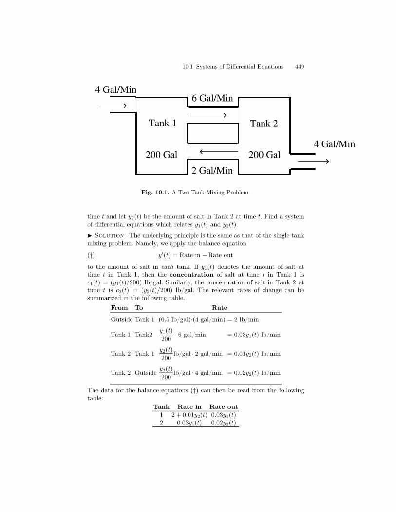
10.1 Systems of Differential Equations 449
Tank 1 Tank 2
200 Gal 200 Gal
6 Gal/Min4 Gal/Min
2 Gal/Min
4 Gal/Min
Fig. 10.1. A Two Tank Mixing Problem.
time t and let y2(t) be the amount of salt in Tank 2 at time t. Find a systemof differential equations which relates y1(t) and y2(t).
I Solution. The underlying principle is the same as that of the single tankmixing problem. Namely, we apply the balance equation
(†) y′(t) = Rate in− Rate out
to the amount of salt in each tank. If y1(t) denotes the amount of salt attime t in Tank 1, then the concentration of salt at time t in Tank 1 isc1(t) = (y1(t)/200) lb/gal. Similarly, the concentration of salt in Tank 2 attime t is c2(t) = (y2(t)/200) lb/gal. The relevant rates of change can besummarized in the following table.
From To Rate
Outside Tank 1 (0.5 lb/gal)·(4 gal/min) = 2 lb/min
Tank 1 Tank2y1(t)
200· 6 gal/min = 0.03y1(t) lb/min
Tank 2 Tank 1y2(t)
200lb/gal · 2 gal/min = 0.01y2(t) lb/min
Tank 2 Outsidey2(t)
200lb/gal · 4 gal/min = 0.02y2(t) lb/min
The data for the balance equations (†) can then be read from the followingtable:
Tank Rate in Rate out1 2 + 0.01y2(t) 0.03y1(t)2 0.03y1(t) 0.02y2(t)
450 10 Systems of Differential Equations
Putting these data in the balance equations then gives
y′1(t) = 2 + 0.01y2(t) − 0.03y1(t)y′2(t) = 0.03y1(t) − 0.02y2(t)
as the first order system of ordinary differential equations satisfied by thevector function whose two components are the amount of salt in tank 1 andin tank 2 at time t. This system is a nonhomogeneous, constant coefficient,linear system. We shall address some techniques for solving such equations inSection 10.4, after first considering some of the theoretical underpinnings ofthese equations in the next two sections. J
Exercises
For each of the following systems of differential equations, determine if it islinear (yes/no) and autonomous (yes/no). For each of those which is linear, fur-ther determine if the equation is homogeneous/nonhomogeneous and constantcoefficient (yes/no). Do not solve the equations.
1.y′1 = y2
y′2 = y1y2
2.y′1 = y1 + y2 + t2
y′2 = −y1 + y2 + 1
3.y′1 = (sin t)y1 − y2
y′2 = y1 + (cos t)y2
4.y′1 = t sin y1 − y2
y′2 = y1 + t cos y2
5.
y′1 = y1
y′2 = 2y1 + y4
y′3 = y4
y′4 = y2 + 2y3
6.y′1 =
1
2y1 − y2 + 5
y′2 = −y1 +
1
2y2 − 5
7. Verify that y(t) = y1(t)y2(t), where y1(t) = et − e3t and y2(t) = 2et − e3t is a
solution of the initial value problem
y′ = 5 −2
4 −1y; y(0) = 01 .
10.1 Systems of Differential Equations 451
Solution: First note that y1(0) = 0 and y2(0) = 1, so the initial condi-
tion is satisfied. Then y′(t) = y′1(t)
y′2(t) = et − 3e3t
2et − 3e3t while 5 −24 −1y(t) =
5(et − e3t) − 2(2et − e3t)4(et − e3t) − (2et − e3t) = et − 3e3t
2et − 3e3t. Thus y′(t) = 5 −24 −1y, as required.
8. Verify that y(t) = y1(t)y2(t), where y1(t) = 2e4t − e−2t and y2(t) = 2e4t + e−2t is
a solution of the initial value problem
y′ = 1 3
3 1y; y(0) = 13 .
9. Verify that y(t) = y1(t)y2(t), where y1(t) = et +2tet and y2(t) = 4tet is a solution
of the initial value problem
y′ = 3 −1
4 −1y; y(0) = 10 .
10. Verify that y(t) = y1(t)y2(t), where y1(t) = cos 2t− 2 sin 2t and y2(t) = − cos 2t is
a solution of the initial value problem
y′ = 1 5
−1 −1y; y(0) = 1−1 .
Rewrite each of the following initial value problems for an ordinary differen-tial equation as an initial value problem for a first order system of ordinarydifferential equations.
11. y′′ + 5y′ + 6y = e2t, y(0) = 1, y′(0) = −2.Solution: Let y1 = y and y2 = y′. Then y′
1 = y′ = y2 and y′2 = y′′ = −5y′ −
6y + e2t = −6y1 − 5y2 + e2t. Letting y = y1
y2, this can be expressed in vector
form (see Equation (6.1.7)) as
y′ = 0 1
−6 −5y + 0e2t ; y(0) = 1
−2 .
12. y′′ + k2y = 0, y(0) = −1, y′(0) = 0
13. y′′ − k2y = 0, y(0) = −1, y′(0) = 0
14. y′′ + k2y = A cos ωt, y(0) = 0, y′(0) = 0
15. ay′′ + by′ + cy = 0, y(0) = α, y′(0) = β
16. ay′′ + by′ + cy = A sin ωt, y(0) = α, y′(0) = β
17. t2y′′ + 2ty′ + y = 0, y(1) = −2, y′(1) = 3
452 10 Systems of Differential Equations
10.2 Linear Systems of Differential Equations
This section and the next will be devoted to the theoretical underpinningsof linear systems of ordinary differential equations which accrue from themain theorem of existence and uniqueness of solutions of such systems. Aswith Picard’s existence and uniqueness theorem (Theorem 2) for first orderordinary differential equations, and the similar theorem for linear second orderequations (Theorem ??), we will not prove this theorem, but rather show howit leads to immediately useful information to assist us in knowing when wehave found all solutions.
A first order system y′ = f (t, y) in standard form is linear providedf(t, y) = A(t)y + q(t) where A(t) = [aij(t)] is an n× n matrix of functions,while
q(t) =
q1(t)...
qn(t)
and y =
y1...yn
are n×1 matrices. Thus the standard description of a first order linear systemin matrix form is
y′ = A(t)y + q(t), (1)
while, if the matrix equation is written out in terms of the unknown functionsy1, y2, . . ., yn, then (1) becomes
y′1 = a11(t)y1 + a12(t)y2 + · · · + a1n(t)yn + q1(t)y′2 = a21(t)y1 + a22(t)y2 + · · · + a2n(t)yn + q2(t). . . . . . . . . . . . . . . . . . . . . . . . . . . . . . . . . . . . . . . . . . . . . . . . .y′n = an1(t)y1 + an2(t)y2 + · · · + ann(t)yn + qn(t).
(2)
For example, the matrix equation
y′ =
[
1 −te−t −1
]
y +
[
cos t0
]
and the system of equations
y′1 = y1 − ty2 + cos t
y′2 = e−ty1 − y2
have the same meaning.It is convenient to state most of our results on linear systems of ordinary
differential equations in the language of matrices and vectors. To this end thefollowing terminology will be useful. A property P of functions will be said tobe satisfied for a matrix A(t) = [aij(t)] of functions if it is satisfied for all ofthe functions aij(t) which make up the matrix. In particular:
1. A(t) is defined on an interval I of R if each aij(t) is defined on I.
10.2 Linear Systems of Differential Equations 453
2. A(t) is continuous on an interval I of R if each aij(t) is continuous onI. For instance, the matrix
A(t) =
1
t+ 2cos 2t
e−2t 1
(2t− 3)2
is continuous on each of the intervals I1 = (−∞,−2), I2 = (−2, 3/2) andI3 = (3/2,∞), but it is not continuous on the interval I4 = (0, 2).
3. A(t) is differentiable on an interval I of R if each aij(t) is differentiableon I. Moreover, A′(t) = [a′ij(t)]. That is, the matrix A(t) is differentiatedby differentiating each entry of the matrix. For instance, for the matrixA(t) in the previous item,
A′(t) =
−1
(t+ 2)2−2 sin2t
−2e−2t −4
(2t− 3)3
.
4. A(t) is integrable on an interval I of R if each aij(t) is integrable on I.Moreover, the integral ofA(t) on the interval [a, b] is computed by comput-
ing the integral of each entry of the matrix, i.e.,∫ b
aA(t) dt =
[
∫ b
aaij(t) dt
]
.
For the matrix A(t) of item 2 above, this gives
∫ 1
0
A(t) dt =
∫ 1
0
1
t+ 2dt
∫ 1
0cos 2t dt
∫ 1
0 e−2t dt
∫ 1
0
1
(2t− 3)2dt
=
[
ln 32
12 sin 2
12 (1− e−2) 1
3
]
,
while, if t ∈ I2 = (−2, 3/2), then
∫ t
0
A(u) du =
∫ t
0
1
u+ 2du
∫ t
0 cos 2u du
∫ t
0e−2u du
∫ 1
0
1
(2u− 3)2du
=
lnt+ 2
212 sin 2t
12 (1− e−2t)
−1
2(2t− 3)− 1
6
.
5. If each entry aij(t) ofA(t) is of exponential type (see the definition on page347), we can take the Laplace transform of A(t), by taking the Laplacetransform of each entry. That is L(A(t))(s) = [L(aij(t))(s)]. For example,
if A(t) =
[
te−2t cos 2te3t sin t (2t− e)2
]
, this gives
L(A(t))(s) =
[
L(
te−2t)
(s) L(cos 2t)(s)
L(e3t sin t)(s) L(
(2t− 3)2)
(s)
]
=
1
(s+ 2)22
s2 + 4
1
(s− 3)2 + 1
8e3t2
s3
.
454 10 Systems of Differential Equations
If A(t) and q(t) are continuous matrix functions on an interval I, then asolution to the linear differential equation
y′ = A(t)y + q(t)
on the subinterval J ⊆ I, is a continuous matrix function y(t) on J such that
y′(t) = A(t)y(t) + q(t)
for all t ∈ J . If moreover, y(t0) = y0, then y(t) is a solution of the initialvalue problem
y′ = A(t)y + q(t), y(t0) = y0. (3)
Example 1. Verify that y(t) =
[
e3t
3e3t
]
is a solution of the initial value
problem (3) on the interval (−∞, ∞) where
A(t) =
[
0 16 −1
]
, q(t) =
[
06e3t
]
, t0 = 0 and y0 =
[
13
]
.
I Solution. All of the functions in the matrices A(t), y(t), and q(t) are
differentiable on the entire real line (−∞, ∞) and y(t0) = y(0) =
[
13
]
= y0.
Moreover,
(∗) y′(t) =
[
3e3t
9e3t
]
and
(∗∗) A(t)y(t) + q(t) =
[
0 16 −1
] [
e3t
3e3t
]
+
[
06e3t
]
=
[
3e3t
9e3t
]
.
Since (∗) and (∗∗) agree, y(t) is a solution of the initial value problem. J
The Existence and Uniqueness Theorem
The following result is the fundamental foundational result of the currenttheory. It is the result which guarantees that if we can find a solution of alinear initial value problem by any means whatsoever, then we know that wehave found the only possible solution.
Theorem 2 (Existence and Uniqueness). 1 Suppose that the n×n matrixfunction A(t) and the n × 1 matrix function q(t) are both continuous on aninterval I in R. Let t0 ∈ I. Then for every choice of the vector y0, the initialvalue problem
y′ = A(t)y + q(t), y(t0) = y0
has a unique solution y(t) which is defined on the same interval I.
1A Proof of this result can be found in the text An Introduction to Ordinary
Differential Equations by Earl Coddington, Prentice-Hall, (1961), Page 256.
10.2 Linear Systems of Differential Equations 455
Remark 3. How is this theorem related to existence and uniqueness theoremswe have stated previously?
• If n = 1 then this theorem is just Corollary 9. In this case we have actuallyproved the result by exhibiting a formula for the unique solution. We arenot so lucky for general n. There is no formula like Equation (7) which isvalid for the solutions of linear initial value problems if n > 1.
• Theorem ?? is a corollary of Theorem 2. Indeed, if n = 2,
A(t) =
[
0 1−b(t) −a(t)
]
,
q(t) =
[
0f(t)
]
, y0 =
[
y0y1
]
, and y =
[
yy′
]
, then the second order linear
initial value problem
y′′ + a(t)y′ + b(t)y = f(t), y(t0) = y0, y′(t0) = y1
has the solution y(t) if and only if the first order linear system
y′ = A(t)y + q(t), y(t0) = y0
has the solution y(t) =
[
y(t)y′(t)
]
. You should convince yourself of the validity
of this statement.
Example 4. Let n = 2 and consider the initial value problem (3) where
A(t) =
−t 1
t+ 11
t2 − 2t2
, q(t) =
[
e−t
cos t
]
, t0 = 0, y0 =
[
12
]
.
Determine the largest interval I on which a solution to (3) is guaranteed byTheorem 2.
I Solution. All of the entries in all the matrices above are continuous on
the entire real line except that1
t+ 1is not continuous for t = −1 and
1
t2 − 2is not continuous for t = ±
√2. Thus the largest interval I containing 0 for
which all of the matrix entries are continuous is I = (−1,√
2). The theoremapplies on this interval, and on no larger interval containing 0. J
For first order differential equations, the Picard approximation algorithm(Algorithm 1) provides an algorithmic procedure for finding an approximatesolution to a first order initial value problem y′ = f(t, y), y′(t0) = y0. For firstorder systems, the Picard approximation algorithm also works. We will statethe algorithm only for linear first order systems and then apply it to constantcoefficient first order systems, where we will be able to see an immediateanalogy to the simple linear equation y′ = ay, y′(0) = c, which, as we knowfrom Chapter 2, has the solution y(t) = ceat.
456 10 Systems of Differential Equations
Algorithm 5 (Picard Approximation for Linear Systems). Performthe following sequence of steps to produce an approximate solution to theinitial value problem (3).
(i) A rough initial approximation to a solution is given by the constant func-tion
y0(t) := y0.
(ii) Insert this initial approximation into the right hand side of Equation (3)and obtain the first approximation
y1(t) := y0 +
∫ t
t0
(A(u)y0(u) + q(u)) du.
(iii)The next step is to generate the second approximation in the same way;i.e.,
y2(t) := y0 +
∫ t
t0
(A(u)y1(u) + q(u)) du.
(iv)At the n-th stage of the process we have
yn(t) := y0 +
∫ t
t0
(A(u)yn−1(u) + q(u)) du,
which is defined by substituting the previous approximation yn−1(t) intothe right hand side of Equation (3).
As in the case of first order equations, under the hypotheses of the Ex-istence and Uniqueness for linear systems, the sequence of vector functionsyn(t) produced by the Picard Approximation algorithm will converge on theinterval I to the unique solution of the initial value problem (3).
Example 6. We will consider the Picard Approximation algorithm in thespecial case where the coefficient matrix A(t) is constant, so that we can writeA(t) = A, the function q(t) = 0, and the initial point t0 = 0. In this case theinitial value problem (3) becomes
y′ = Ay, y(0) = y0, (4)
and we get the following sequence of Picard approximations yn(t) to thesolution y(t) of (4).
10.2 Linear Systems of Differential Equations 457
y0(t) = y0
y1(t) = y0 +
∫ t
0
Ay0 du
= y0 +Ay0t
y2(t) = y0 +
∫ t
0
Ay1(u) du
= y0 +
∫ t
0
A(y0 +Ay0u) du
= y0 +Ay0t+1
2A2y0t
2
y3(t) =
∫ t
0
A
(
y0 +Ay0u+1
2A2y0u
2
)
du
= y0 +Ay0t+1
2A2y0t
2 +1
6A3y0t
3
...
yn(t) = y0 +Ay0t+1
2A2y0t
2 + · · ·+ 1
n!Any0t
n.
Notice that we may factor a y0 out of each term on the right hand side ofyn(t). This gives the following expression for the function yn(t):
yn(t) =
(
In +At+1
2A2t2 +
1
3!A3t3 + · · ·+ 1
n!Antn
)
y0 (5)
where In denotes the identity matrix of size n. If you recall the Taylor seriesexpansion for the exponential function eat:
eat = 1 + at+1
2(at)2 +
1
3!(at)3 + · · ·+ 1
n!(at)n + · · ·
you should immediately see a similarity. If we replace the scalar a with then×n matrix A and the scalar 1 with the identity matrix In then we can defineeAt to be the sum of the resulting series. That is,
eAt = In +At+1
2(At)2 +
1
3!(At)3 + · · ·+ 1
n!(At)n + · · · . (6)
It is not difficult (but we will not do it) to show that the series we havewritten down for defining eAt in fact converges for any n × n matrix A, andthe resulting sum is an n× n matrix of functions of t. That is
eAt =
h11(t) h12(t) · · · h1n(t)h21(t) h22(t) · · · h2n(t)
......
. . ....
hn1(t) hn2(t) · · · hnn(t)
.
458 10 Systems of Differential Equations
It is not, however, obvious what the functions hij(t) are. Much of the remain-der of this chapter will be concerned with precisely that problem. For now, wesimply want to observe that the functions yn(t) (see Equation (5)) computedfrom the Picard approximation algorithm converge to eAty0, that is the ma-trix function eAt multiplied by the constant vector y0 from the initial valueproblem (4). Hence we have arrived at the following fact: The unique solutionto (4) is
y(t) = eAty0. (7)
Following are a few examples where we can compute the matrix exponentialeAt with only the definition.
Example 7. Compute eAt for each of the following constant matrices A.
1. A =
[
0 00 0
]
= 02. (In general 0k denotes the k × k matrix, all of whose
entries are 0.)
I Solution. In this case Antn =
[
0 00 0
]
for all n. Hence,
e02t = eAt = I2 +At+1
2A2t2 +
1
3!A3t3 + · · ·
= I2 + 02 + 02 + · · ·= I2.
Similarly, e0nt = In. This is the matrix analog of the fact e0 = 1. J
2. A =
[
2 00 3
]
.
I Solution. In this case the powers of the matrix A are easy to compute.In fact
A2 =
[
4 00 9
]
, A3 =
[
8 00 27
]
, · · · An =
[
2n 00 3n
]
,
so that
eAt = I +At+1
2A2t2 +
1
3!A3t3 + · · ·
=
[
1 00 1
]
+
[
2t 00 3t
]
+1
2
[
4t2 00 9t2
]
+
+1
3!
[
8t3 00 27t3
]
+ · · ·+ 1
n!
[
2ntn 00 3ntn
]
+ · · ·
=
[
1 + 2t+ 124t2 + · · ·+ 1
n!2ntn + · · · 0
0 1 + 3t+ 129t2 + · · ·+ 1
n!3ntn + · · ·
]
=
[
e2t 00 e3t
]
.
10.2 Linear Systems of Differential Equations 459
J
3. A =
[
a 00 b
]
.
I Solution. There is clearly nothing special about the numbers 2 and 3on the diagonal of the matrix in the last example. The same calculationshows that
eAt = e "#a 00 b$%t
=
[
eat 00 ebt
]
. (8)
J
4. A =
[
0 10 0
]
.
I Solution. In this case, check that A2 =
[
0 10 0
] [
0 10 0
]
=
[
0 00 0
]
= 02.
Then An = 02 for all n ≥ 2. Hence,
eAt = I +At+1
2A2t2 +
1
3!A3t3 + · · ·
= I +At
=
[
1 t0 1
]
.
Note that in this case, the individual entries of eAt do not look like expo-nential functions eat at all. J
5. A =
[
0 −11 0
]
.
I Solution. We leave it as an exercise to compute the powers of the
matrix A. You should find A2 =
[
−1 00 −1
]
, A3 =
[
0 1−1 0
]
, A4 =
[
1 00 1
]
= I2,
A5 = A, A6 = A2, etc. That is, the powers repeat with period 4. Then
eAt = I +At+1
2A2t2 +
1
3!A3t3 + · · ·
=
[
1 00 1
]
+
[
0 −tt 0
]
+1
2
[
−t2 00 −t2
]
+1
3!
[
0 t3
−t3 0
]
+1
4!
[
t4 00 t4
]
+ · · ·
=
1− 12 t
2 + 14! t
4 + · · · −t+ 13! t
3 − 15! t
5 + · · ·
t− 13! t
3 + 15! t
5 − · · · 1− 12 t
2 + 14! t
4 + · · ·
=
[
cos t − sin tsin t cos t
]
.
460 10 Systems of Differential Equations
In this example also the individual entries of eAt are not themselves ex-ponential functions. J
Example 8. Use Equation (7) and the calculation of eAt from the corre-sponding item in the previous example to solve the initial value problem
y′ = Ay, y(0) = y0 =
[
c1c2
]
for each of the following matrices A.
1. A =
[
0 00 0
]
= 02.
I Solution. By Equation (7), the solution y(t) is given by
y(t) = eAty0 = I2y0 = y0 =
[
c1c2
]
. (9)
That is, the solution of the vector differential equation y′ = 0, y(0) = y0
is the constant function y(t) = y0. In terms of the component functionsy1(t), y2(t), the system of equations we are considering is
y′1 = 0, y1(0) = c1
y′2 = 0, y2(0) = c2
and this clearly has the solution y1(t) = c1, y2(t) = c2, which agrees with(9). J
2. A =
[
2 00 3
]
.
I Solution. Since in this case, eAt =
[
e2t 00 e3t
]
, the solution of the initial
value problem is
y(t) = eAty0 =
[
e2t 00 e3t
] [
c1c2
]
=
[
c1e2t
c2e3t
]
.
Again, in terms of the component functions y1(t), y2(t), the system ofequations we are considering is
y′1 = 2y1, y1(0) = c1
y′2 = 3y2, y2(0) = c2.
Since the first equation does not involve y2 and the second equation doesnot involve y1, what we really have is two independent first order linearequations. The first equation clearly has the solution y1(t) = c1e
2t and thesecond clearly has the solution y2(t) = c2e
3t, which agrees with the vectordescription provided by Equation (7). (If the use of the word clearly is notclear, then you are advised to review Section 2.2.) J
10.2 Linear Systems of Differential Equations 461
3. A =
[
a 00 b
]
.
I Solution. Since in this case, eAt =
[
eat 00 ebt
]
, the solution of the initial
value problem is
y(t) = eAty0 =
[
eat 00 ebt
] [
c1c2
]
=
[
c1eat
c2ebt
]
.
J
4. A =
[
0 10 0
]
.
I Solution. In this case eAt =
[
1 t0 1
]
, so the solution of the initial value
problem is
y(t) = eAty0 =
[
1 t0 1
] [
c1c2
]
=
[
c1 + tc2c2
]
.
Again, for comparative purposes, we will write this equation as a systemof two equations in two unknowns:
y′1 = y2, y1(0) = c1
y′2 = 0, y2(0) = c2.
In this case also, it is easy to see directly what the solution of the system isand to see that it agrees with that computed by Equation (7). Indeed, thesecond equation says that y2(t) = c2, and then the first equation impliesthat y1(t) = c1 + tc2 by integration.
J
5. A =
[
0 −11 0
]
.
I Solution. The solution of the initial value problem is
y(t) = eAty0 =
[
cos t − sin tsin t cos t
] [
c1c2
]
=
[
c1 cos t− c2 sin tc1 sin t+ c2 cos t
]
.
J
Exercises
Compute the derivative of each of the following matrix functions.
1. A(t) = cos 2t sin 2t− sin 2t cos 2t
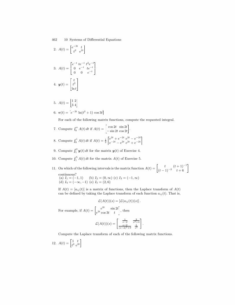
462 10 Systems of Differential Equations
2. A(t) = e−3t tt2 e2t
3. A(t) = e−t te−t t2e−t
0 e−t te−t
0 0 e−t 4. y(t) = t
t2
ln t5. A(t) = 1 2
3 46. v(t) = e−2t ln(t2 + 1) cos 3t!
For each of the following matrix functions, compute the requested integral.
7. Compute π
0A(t) dt if A(t) = cos 2t sin 2t
− sin 2t cos 2t.8. Compute
1
0A(t) dt if A(t) = 1
2 e2t + e−2t e2t − e−2t
e−2t − e2t e2t + e−2t9. Compute
2
1y(t) dt for the matrix y(t) of Exercise 4.
10. Compute 5
1A(t) dt for the matrix A(t) of Exercise 5.
11. On which of the following intervals is the matrix function A(t) = t (t + 1)−1
(t − 1)−2 t + 6 continuous?(a) I1 = (−1, 1) (b) I2 = (0,∞) (c) I3 = (−1,∞)(d) I4 = (−∞,−1) (e) I5 = (2, 6)
If A(t) = [aij(t)] is a matrix of functions, then the Laplace transform of A(t)can be defined by taking the Laplace transform of each function aij(t). That is,
L(A(t))(s) = [L(aij(t))(s)] .
For example, if A(t) = e2t sin 2te2t cos 3t t , then
L(A(t))(s) = & 1s−2
2s2+4
s−2(s−2)2+9
1s2 ' .
Compute the Laplace transform of each of the following matrix functions.
12. A(t) = 1 tt2 e2t
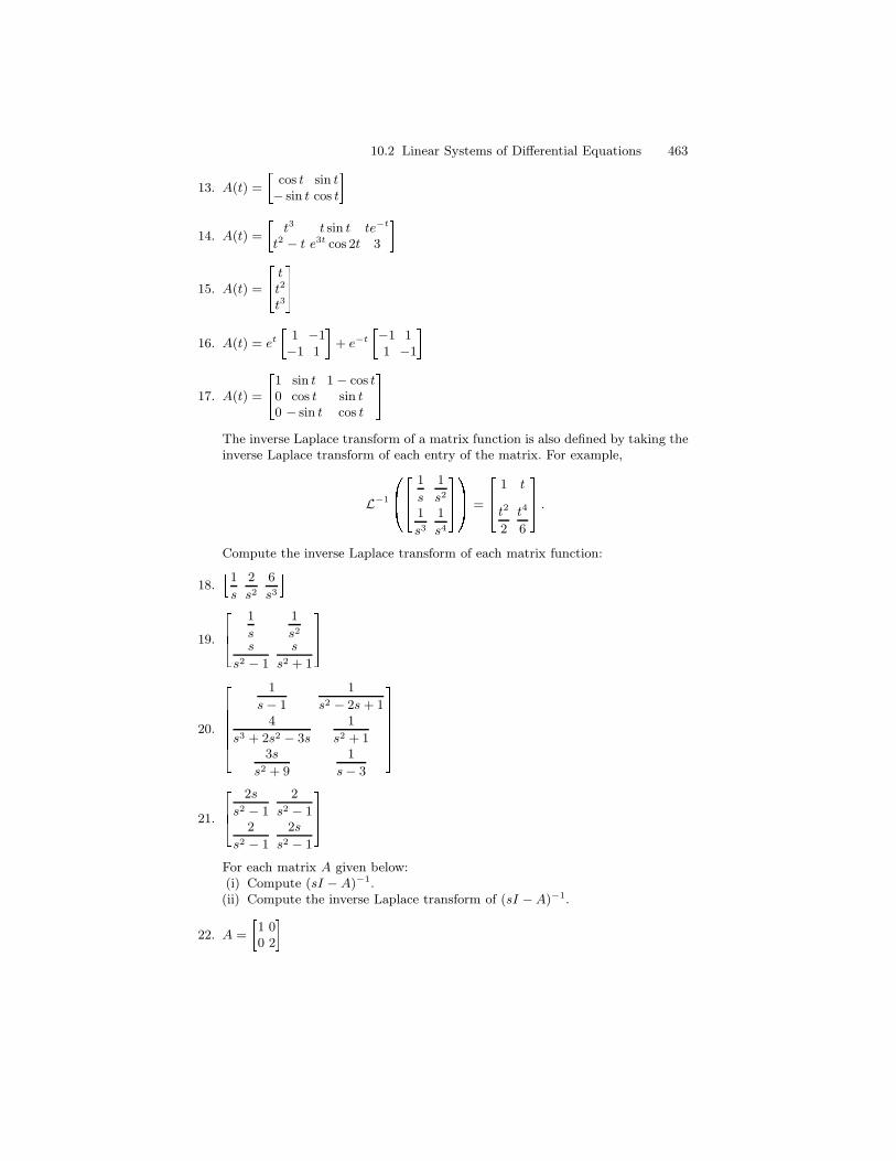
10.2 Linear Systems of Differential Equations 463
13. A(t) = cos t sin t− sin t cos t
14. A(t) = t3 t sin t te−t
t2 − t e3t cos 2t 3 15. A(t) = t
t2
t316. A(t) = et 1 −1
−1 1 + e−t −1 11 −1
17. A(t) = 1 sin t 1 − cos t0 cos t sin t0 − sin t cos t
The inverse Laplace transform of a matrix function is also defined by taking theinverse Laplace transform of each entry of the matrix. For example,
L−1 ()*1
s
1
s2
1
s3
1
s4+,- = 1 t
t2
2
t4
6 .
Compute the inverse Laplace transform of each matrix function:
18. .1s
2
s2
6
s3 /19. 1
s
1
s2
s
s2 − 1
s
s2 + 1
20.
1
s − 1
1
s2 − 2s + 14
s3 + 2s2 − 3s
1
s2 + 13s
s2 + 9
1
s − 3
21. 2s
s2 − 1
2
s2 − 12
s2 − 1
2s
s2 − 1
For each matrix A given below:(i) Compute (sI − A)−1.(ii) Compute the inverse Laplace transform of (sI − A)−1.
22. A = 1 00 2
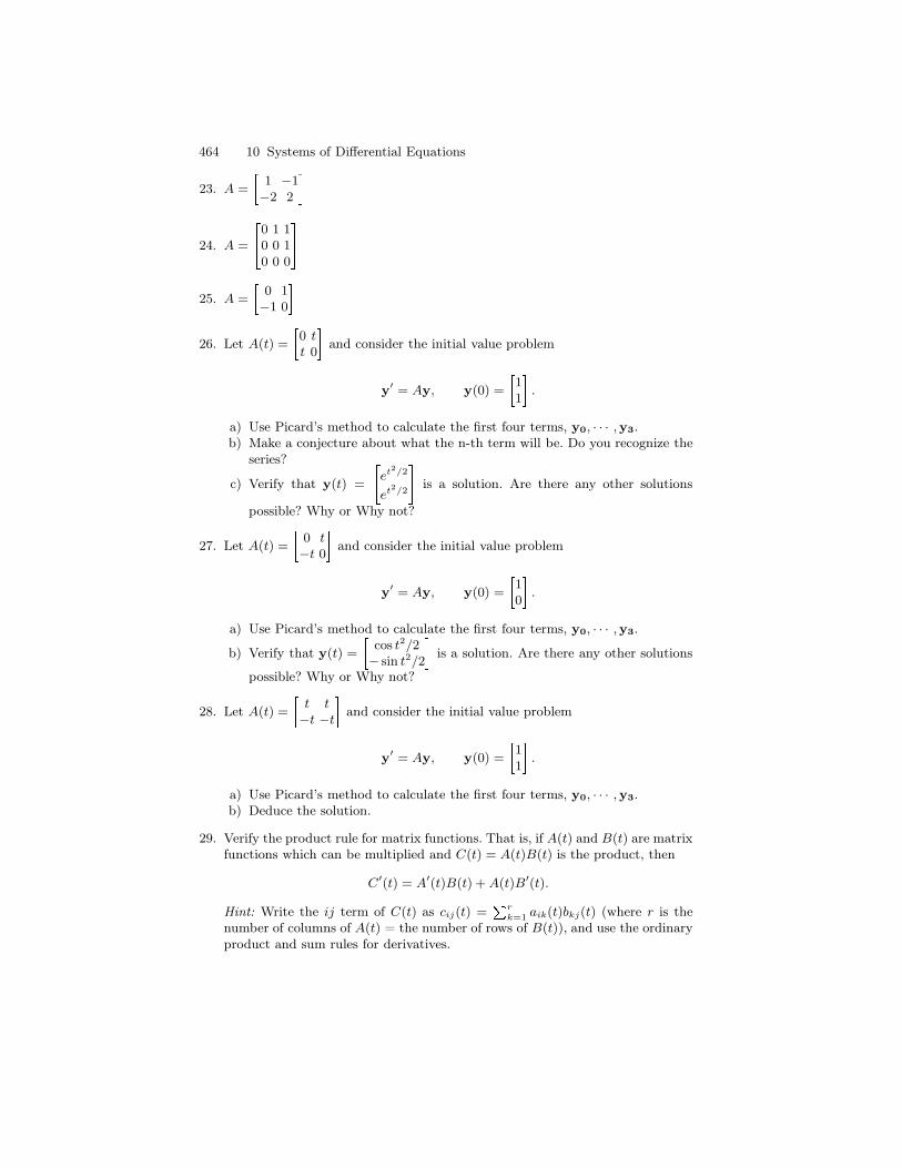
464 10 Systems of Differential Equations
23. A = 1 −1−2 2
24. A = 0 1 10 0 10 0 0
25. A = 0 1−1 0
26. Let A(t) = 0 tt 0 and consider the initial value problem
y′ = Ay, y(0) = 11 .
a) Use Picard’s method to calculate the first four terms, y0, · · · ,y3.b) Make a conjecture about what the n-th term will be. Do you recognize the
series?
c) Verify that y(t) = &et2/2
et2/2' is a solution. Are there any other solutions
possible? Why or Why not?
27. Let A(t) = 0 t−t 0 and consider the initial value problem
y′ = Ay, y(0) = 10 .
a) Use Picard’s method to calculate the first four terms, y0, · · · ,y3.
b) Verify that y(t) = cos t2/2− sin t2/2 is a solution. Are there any other solutions
possible? Why or Why not?
28. Let A(t) = t t−t −t and consider the initial value problem
y′ = Ay, y(0) = 11 .
a) Use Picard’s method to calculate the first four terms, y0, · · · ,y3.b) Deduce the solution.
29. Verify the product rule for matrix functions. That is, if A(t) and B(t) are matrixfunctions which can be multiplied and C(t) = A(t)B(t) is the product, then
C′(t) = A′(t)B(t) + A(t)B′(t).
Hint: Write the ij term of C(t) as cij(t) =r
k=1 aik(t)bkj(t) (where r is thenumber of columns of A(t) = the number of rows of B(t)), and use the ordinaryproduct and sum rules for derivatives.
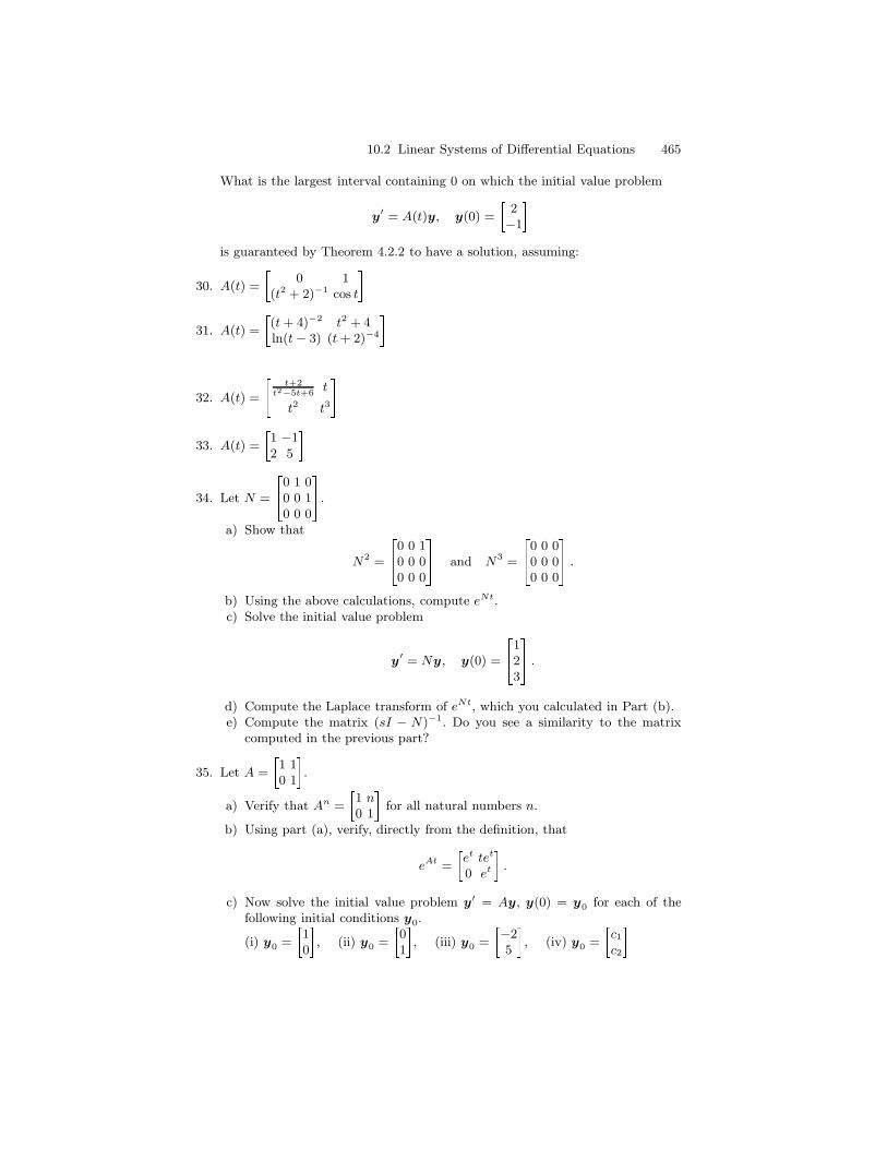
10.2 Linear Systems of Differential Equations 465
What is the largest interval containing 0 on which the initial value problem
y′ = A(t)y, y(0) = 2
−1is guaranteed by Theorem 4.2.2 to have a solution, assuming:
30. A(t) = 0 1(t2 + 2)−1 cos t
31. A(t) = (t + 4)−2 t2 + 4ln(t − 3) (t + 2)−4
32. A(t) = & t+2t2−5t+6
t
t2 t3'33. A(t) = 1 −1
2 5 34. Let N = 0 1 0
0 0 10 0 0.
a) Show that
N2 = 0 0 10 0 00 0 0 and N3 = 0 0 0
0 0 00 0 0 .
b) Using the above calculations, compute eNt.c) Solve the initial value problem
y′ = Ny, y(0) = 12
3 .
d) Compute the Laplace transform of eNt, which you calculated in Part (b).e) Compute the matrix (sI − N)−1. Do you see a similarity to the matrix
computed in the previous part?
35. Let A = 1 10 1.
a) Verify that An = 1 n0 1 for all natural numbers n.
b) Using part (a), verify, directly from the definition, that
eAt = et tet
0 et .
c) Now solve the initial value problem y′ = Ay, y(0) = y0 for each of thefollowing initial conditions y0.
(i) y0 = 10, (ii) y0 = 01, (iii) y0 = −25 , (iv) y0 = c1
c2
466 10 Systems of Differential Equations
d) Compute the Laplace transform of eAt.e) Compute (sI − A)−1 and compare to the matrix computed in Part (d).
36. One of the fundamental properties of the exponential function is the formulaea+b = eaeb. The goal of this exercise is to show, by means of a concrete ex-ample, that the analog of this fundamental formula is not true for the matrixexponential function (at least without some additional assumptions). From the
calculations of Example 4.2.7, you know that if A = 2 00 3 and B = 0 1
0 0, then
eAt = e2t 00 e3t and eBt = 1 t
0 1.a) Show that eAteBt = e2t te3t
0 e3t .b) Let y0 = 01 and let y(t) = eAteBty0. Compute y′(t) and (A + B)y(t).
Are these two functions the same?c) What do these calculations tell you about the possible equality of the matrix
functions eAteBt and e(A+B)t for these particular A and B?d) We will see later that the formula e(A+B)t = eAteBt is valid provided that
AB = BA. Check that AB 6= BA for the matrices of this exercise.
10.3 Linear Homogeneous Equations
This section will be concerned with using the fundamental existence anduniqueness theorem for linear systems (Theorem 2) to describe the solutionset for a linear homogeneous system of ordinary differential equations
y′ = A(t)y. (1)
The main result will be similar to the description given by Theorem ?? forlinear homogeneous second order equations.
Recall that if A(t) is a continuous n × n matrix function on an intervalI, then a solution to system (1) is an n × 1 matrix function y(t) such thaty′(t) = A(t)y(t) for all t ∈ I. Since this is equivalent to the statement
y′(t)−A(t)y(t) = 0 for all t ∈ I,
to be consistent with the language of solution sets used in Chapter 6, we willdenote the set of all solutions of (1) by S0
L, where L = D−A(t) is the (vector)
differential operator which acts on the vector function y(t) by the rule
L(y(t)) = (D −A(t))(y(t)) = y′(t)−A(t)y(t).
Thus
10.3 Linear Homogeneous Equations 467
S0L
= y(t) : L(y(t)) = 0 .Let y1(t) and y2(t) be two solutions of system (1), i.e., y1(t) and y2(t)
are in S0L
and let y(t) = c1y1(t) + c2y2(t) where c1 and c2 are scalars (eitherreal or complex). Then
y′(t) = (c1y1(t) + c2y2(t))′
= c1y′1(t) + c2y
′2(t)
= c1A(t)y1(t) + c2A(t)y2(t)
= A(t) (c1y1(t) + c2y2(t))
= A(t)y(t).
Thus every linear combination of two solutions of (1) is again a solution. whichin the language of linear algebra means that S0
Lis a vector space. We say
that a set of vectorsB = v1, . . . , vk
in a vector space V is a basis of V if the set B is linearly independent andif every vector v in V can be written as a linear combination
v = λ1v1 + · · ·+ λkvk.
The number k of vectors in a basis B of V is known as the dimension ofV . Thus R2 has dimension 2 since it has a basis e1 = (1, 0), e2 = (0, 1)consisting of 2 vectors, R3 has dimension 3 since it has a basis e1 = (1, 0, 0),e2 = (0, 1, 0), e3 = (0, 0, 1) consisting of 3 vectors, etc. The main theorem onsolutions of linear homogeneous systems can be expressed most convenientlyin the language of vector spaces.
Theorem 1. If the n×n matrix A(t) is continuous on an interval I, then thesolution set S0
Lof the homogeneous system
y′ = A(t)y (2)
is a vector space of dimension n. In other words,
1. There are n linearly independent solutions of (2) in S0L.
2. If ϕ1, ϕ2, . . ., ϕn ∈ S0L
are independent solutions of (2), and ϕ is anyfunction in S0
L, then ϕ can be written as
ϕ = c1ϕ1 + · · ·+ cnϕn
for some scalars c1, . . ., cn ∈ R.
Proof. To keep the notation as explicit as possible, we will only present theproof in the case n = 2. You should compare this proof with that of Theorem??. To start with, let
468 10 Systems of Differential Equations
e1 =
[
10
]
and e2 =
[
01
]
,
and let t0 ∈ I. By Theorem 2 there are vector functions ψ1(t) and ψ2(t)defined for all t ∈ I and which satisfy the initial conditions
ψi(t0) = ei for i = 1, 2. (3)
Suppose there is a dependence relation c1ψ1 + c2ψ2 = 0. This means that
c1ψ1(t) + c2ψ2(t) = 0
for all t ∈ I. Applying this equation to the particular point t0 gives
0 = c1ψ1(t0) + c2ψ2(t0) = c1e1 + c2e2 = c1
[
10
]
+ c2
[
01
]
=
[
c1c2
]
.
Thus c1 = 0 and c2 = 0 so that ψ1 and ψ2 are linearly independent. Thisproves (1).
Now suppose that ϕ ∈ S0L. Evaluating at t0 gives
ϕ(t0) =
[
rs
]
.
Now define ψ ∈ S0L
by ψ = rψ1 +sψ2. Note that ψ ∈ S0L
since S0L
is a vectorspace. Moreover,
ψ(t0) = rψ1(t0) + sψ2(t0) = re1 + se2 =
[
rs
]
= ϕ(t0).
This means that ϕ and ψ = rψ1 + sψ2 are two elements of S0L
which havethe same value at t0. By the uniqueness part of Theorem 2, they are equal.
Now suppose that ϕ1 and ϕ2 are any two linearly independent solutionsof (2) in S0
L. From the argument of the previous paragraph, there are scalars
a, b, c, d so that
ϕ1 = aψ1 + bψ2
ϕ2 = cψ1 + dψ2
which in matrix form can be written
[
ϕ1 ϕ2
]
=[
ψ1 ψ2
]
[
a cb d
]
.
We multiply both sides of this matrix equation on the right by the adjoint[
d −c−b a
]
to obtain
[
ϕ1 ϕ2
]
[
d −c−b a
]
=[
ψ1 ψ2
]
[
ad− bc 00 ad− bc
]
=[
ψ1 ψ2
]
(ad− bc).
10.3 Linear Homogeneous Equations 469
Suppose ad− bc = 0. Then
dϕ1 − bϕ2 = 0
and − cϕ1 + aϕ2 = 0.
But since ϕ1 and ϕ2 are independent this implies that a, b, c, and d are zerowhich in turn implies that ϕ1 and ϕ2 are both zero. But this cannot be. Weconclude that ad − bc 6= 0. We can now write ψ1 and ψ2 each as a linearcombination of ϕ1 and ϕ2. Specifically,
[
ψ1 ψ2
]
=1
ad− bc[
ϕ1 ϕ2
]
[
d −c−b a
]
.
Since ϕ is a linear combination of ψ1 and ψ2 it follows that ϕ is a linearcombination of ϕ1 and ϕ2. ut
The matrix
[
a cb d
]
that appears in the above proof is a useful theoreti-
cal criterion for determining if a pair of solutions ϕ1, ϕ2 in S0L
is linearlyindpependent and hence a basis in the case n = 2. The proof shows:
1.[
ϕ1(t0) ϕ2(t0)]
=
[
a cb d
]
2. If the solutions ϕ1(t), ϕ2(t) are a basis of S0L, then ad−bc = det
[
a cb d
]
6= 0,
and moreover, this is true for any t0 ∈ I.3. The converse of the above statement is also true (and easy). Namely, if
det[
ϕ1(t0) ϕ2(t0)]
6= 0
for some t0 ∈ I, then ϕ1, ϕ2 in S0L
is a basis of the solution space (alwaysassuming n = 2).
Now assume that ϕ1 and ϕ2 are any two solutions in S0L. Then we can
form a 2× 2 matrix of functions
Φ(t) =[
ϕ1(t) ϕ2(t)]
where each column is a solution to y′ = A(t)y. We will say that Φ(t) is afundamental matrix for y′ = A(t)y if the columns are linearly independent,and hence form a basis of S0
L. Then the above discussion is summarized in
the following result.
Theorem 2. If A(t) is a 2 × 2 matrix of continuous functions on I, and ifΦ(t) =
[
ϕ1(t) ϕ2(t)]
where each column is a solution to y′ = A(t)y, thenΦ(t) is a fundamental matrix for y′ = A(t)y if and only if detΦ(t) 6= 0 forat least one t ∈ I. If this is true for one t ∈ I, it is in fact true for all t ∈ I.
470 10 Systems of Differential Equations
Remark 3. The above theorem is also true, although we will not prove it,for n× n matrix systems y′ = A(t)y, where a solution matrix consists of ann× n matrix
Φ(t) =[
ϕ1(t) · · · ϕn(t)]
where each column ϕi(t) is a solution to y′ = A(t)y. Then Φ(t) is a funda-mental matrix, that is the columns are a basis for S0
Lif and only if detΦ(t) 6= 0
for at least one t ∈ I.
Note that if a matrix B is written in columns, say
B =[
b1 · · · bn]
,
then the matrix multiplication AB, if it is defined (which means the numberof columns of A is the number of rows of B), can be written as
AB = A[
b1 · · · bn]
=[
Ab1 · · · Abn]
.
In other words, multiply A by each column of B separately. For example, if
A =
[
1 −12 3
]
and B =
[
1 0 20 1 −1
]
,
then
AB =
[
1 −12 3
] [
1 0 20 1 −1
]
=
[[
1 −12 3
] [
10
] [
1 −12 3
] [
01
] [
1 −12 3
] [
2−1
]]
=
[
1 −1 32 3 1
]
.
Now suppose that Φ(t) =[
ϕ1(t) · · · ϕn(t)]
is a fundamental matrix ofsolutions for y′ = A(t)y. Then
Φ′(t) =[
ϕ′1(t) · · · ϕ′
n(t)]
=[
A(t)ϕ1(t) · · · A(t)ϕn(t)]
= A(t)[
ϕ1(t) · · · ϕn(t)]
= A(t)Φ(t).
Thus the n × n matrix Φ(t) satisfies the same differential equation, namelyy′ = A(t)y, as each of its columns. We summarize this discussion in thefollowing theorem.
Theorem 4. If A(t) is a continuous n×n matrix of functions on an intervalI, then an n × n matrix of functions Φ(t) is a fundamental matrix for thehomogeneous linear equation y′ = A(t)y if and only if
10.3 Linear Homogeneous Equations 471
Φ′(t) = A(t)Φ(t)and detΦ(t) 6= 0.
(4)
The second condition need only be checked for one value of t ∈ I.
Example 5. Show that
Φ(t) =
[
e2t e−t
2e2t −e−t
]
is a fundamental matrix for the system y′ =
[
0 12 1
]
y.
I Solution. First check that Φ(t) is a solution matrix, i.e., check that thefirst condition of Equation (4) is satisfied. To see this, we calculate
Φ′(t) =
[
e2t e−t
2e2t −e−t
]′=
[
2e2t −e−t
4e2t e−t
]
and[
0 12 1
]
Φ(t) =
[
0 12 1
] [
e2t e−t
2e2t −e−t
]
=
[
2e2t −e−t
4e2t e−t
]
.
Since these two matrices of functions are the same, Φ(t) is a solution matrix.To check that it is a fundamental matrix, pick t = 0 for example. Then
Φ(0) =
[
1 12 −1
]
and this matrix has determinant −3, so Φ(t) is a fundamental matrix. J
Example 6. Show that
Φ(t) =
[
te2t (t+ 1)e2t
e2t e2t
]
is a fundamental matrix for the system y′ =
[
2 10 2
]
y.
I Solution. Again we check that the two conditions of Equation (4) aresatisfied. First we calculate Φ′(t):
Φ′(t) =
[
te2t (t+ 1)e2t
e2t e2t
]′=
[
(2t+ 1)e2t (2t+ 3)e2t
2e2t 2e2t
]
.
Next we calculate A(t)Φ(t) where A(t) =
[
2 10 2
]
:
[
2 10 2
] [
te2t (t+ 1)e2t
e2t e2t
]
=
[
(2t+ 1)e2t (2t+ 3)e2t
2e2t 2e2t
]
.
472 10 Systems of Differential Equations
Since these two matrices of functions are the same, Φ(t) is a solution matrix.Next check the second condition of (4) at t = 0:
detΦ(0) = det
[
0 11 1
]
= −1 6= 0.
Hence Φ(t) is a fundamental matrix for y′ =
[
2 10 2
]
y. J
Example 7. Show that
Φ(t) =
[
t2 t3
2t 3t2
]
is a fundamental matrix for the system y′ = A(t)y where
A(t) =
[
0 1
− 6
t24
t
]
.
I Solution. Note that
Φ′(t) =
[
2t 3t2
2 6t
]
=
[
0 1
− 6
t24
t
]
[
t2 t3
2t 3t2
]
,
while
detΦ(1) =
[
1 12 3
]
= 1 6= 0.
Hence Φ(t) is a fundamental matrix. Note that Φ(0) =
[
0 00 0
]
which has deter-
minant 0. Why does this not prevent Φ(t) from being a fundamental matrix?J
In Exercise 29, Page 464 you were asked to verify the product rule fordifferentiating a product of matrix functions. The rule is
(B(t)C(t))′ = B′(t)C(t) +B(t)C′(t).
Since matrix multiplication is not commutative, it is necessary to be careful ofthe order. If one of the matrices is constant, then the product rule is simpler:
(B(t)C)′ = B′(t)C
since C′ = 0 for a constant matrix. We apply this observation in the followingway. Suppose that Φ1(t) is a fundamental matrix of a homogeneous systemy′ = A(t)y where A(t) is an n × n matrix of continuous functions on aninterval I. According to Theorem 4 this means that
Φ′1(t) = A(t)Φ1(t) and detΦ1(t) 6= 0.
10.3 Linear Homogeneous Equations 473
Now define a new n × n matrix of functions Φ2(t) := Φ1(t)C where C is ann× n constant matrix. Then
Φ′2(t) = (Φ1(t)C)′ = Φ′
1(t)C = A(t)Φ1(t)C = A(t)Φ2(t),
so that Φ2(t) is a solution matrix for the homogeneous system y′ = A(t)y.To determine if Φ2(t) is also a fundamental matrix, it is only necessary tocompute the determinant:
detΦ2(t) = det(Φ1(t)C) = detΦ1(t) detC.
Since detΦ1(t) 6= 0, it follows that detΦ2(t) 6= 0 if and only if detC 6= 0, i.e.,if and only if C is a nonsingular n× n matrix.
Example 8. In Example 5 it was shown that
Φ(t) =
[
e2t e−t
2e2t −e−t
]
is a fundamental matrix for the system y′ =
[
0 12 1
]
y. Let C = 13
[
1 12 −1
]
. Then
detC = −1/3 6= 0 so C is invertible, and hence
Ψ (t) = Φ(t)C =1
3
[
e2t e−t
2e2t −e−t
] [
1 12 −1
]
=1
3
[
e2t + 2e−t e2t − e−t
2e2t − 2e−t 2e2t + e−t
]
is also a fundamental matrix for y′ =
[
0 12 1
]
y. Note that Ψ (t) has the partic-
ularly nice feature that its value at t = 0 is
Ψ (0) =
[
1 00 1
]
= I2
the 2× 2 identity matrix. ut
Example 9. In Example 6 it was shown that
Φ(t) =
[
te2t (t+ 1)e2t
e2t e2t
]
is a fundamental matrix for the system y′ =
[
2 10 2
]
y. Let C =
[
−1 11 0
]
. Then
detC = −1 6= 0 so C is invertible, and hence
Ψ (t) = Φ(t)C =
[
te2t (t+ 1)e2t
e2t e2t
] [
−1 11 0
]
=
[
e2t te2t
0 e2t
]
is also a fundamental matrix for y′ =
[
2 10 2
]
y. As in the previous example
Ψ (0) = I2 is the identity matrix. ut
474 10 Systems of Differential Equations
If Φ(t) is a fundamental matrix for the linear system y′ = A(t)y on theinterval I and t0 ∈ I, then Φ(t0) is an invertible matrix by Theorem 4 so ifwe take C = (Φ(t0))
−1, then
Ψ (t) = Φ(t)C = Φ(t)(Φ(t0))−1
is a fundamental matrix which satisfies the extra condition
Ψ (t0) = Φ(t0)(Φ(t0))−1 = In.
Hence, we can always arrange for our fundamental matrices to be the identityat the initial point t0. Moreover, the uniqueness part of the existence anduniqueness theorem insures that there is only one solution matrix satisfyingthis extra condition. We record this observation in the following result.
Theorem 10. If A(t) is a continuous n×n matrix of functions on an intervalI and t0 ∈ I, then there is an n× n matrix of functions Ψ (t) such that
1. Ψ (t) is a fundamental matrix for the homogeneous linear equation y′ =A(t)y and
2. Ψ (t0) = In,3. Moreover, Ψ (t) is uniquely determined by these two properties.4. If y0 is a constant vector, then y(t) = Ψ (t)y0 is the unique solution of
the homogeneous initial value problem y′ = A(t)y, y(t0) = y0.
Proof. Only the last statement was not discussed in the preceding paragraphs.Suppose that Ψ (t) satisfies conditions (1) and (2) and let y(t) = Ψ (t)y0. Theny(t0) = Ψ (t0)y0 = Iny0 = y0. Moreover,
y′(t) = Ψ ′(t)y0 = A(t)Ψ (t)y0 = A(t)y(t),
so y(t) is a solution of the initial value problem, as required. ut
Example 11. Solve the initial value problem y′ =
[
0 12 1
]
y, y(0) =
[
3−6
]
.
I Solution. In Example 8 we found a fundamental matrix for y′ =
[
0 12 1
]
y
satisfying (1) and (2) of the above theorem, namely
Ψ (t) =1
3
[
e2t + 2e−t e2t − e−t
2e2t − 2e−t 2e2t + e−t
]
.
Hence the unique solution of the initial value problem is
y(t) = Ψ (t)
[
3−6
]
=1
3
[
e2t + 2e−t e2t − e−t
2e2t − 2e−t 2e2t + e−t
] [
3−6
]
=
[
−e2t + 4e−t
−2e2t − 4e−t
]
.
J
10.3 Linear Homogeneous Equations 475
Example 12. Solve the initial value problem y′ =
[
2 10 2
]
y, y(0) =
[
−23
]
.
I Solution. In Example 9 we found a fundamental matrix for y′ =
[
2 10 2
]
y
satisfying (1) and (2) of the above theorem, namely
Ψ (t) =
[
e2t te2t
0 e2t
]
.
Hence the solution of the initial value problem is
y(t) = Ψ (t)
[
−23
]
=
[
e2t te2t
0 e2t
] [
−23
]
=
[
(3t− 2)e2t
3e2t
]
.
J
We conclude this section by observing that for a constant matrix functionA(t) = A, at least in principle, it is easy to describe the fundamental matrixΨ (t) from Theorem 10. It is in fact the matrix function we have alreadyencountered in the last section, i.e., the matrix exponential eAt. Recall thateAt (for a constant matrix A) is defined by substituting A for a in the Taylorseries expansion of eat:
(∗) eAt = In +At+1
2A2t2 +
1
3!A3t3 + · · ·+ 1
n!Antn + · · ·
We have already observed (but not proved) that the series on the right handside of (∗) converges to a well defined matrix function for all matrices A. LetΨ (t) = eAt. If we set t = 0 in the series we obtain Ψ (0) = eA0 = In and ifwe differentiate the series terms by term (which can be shown to be a validoperation), we get
Ψ ′(t) =d
dteAt
= 0 +A+A2t+1
2A3t2 + · · ·+ 1
(n− 1)!Antn−1 + · · ·
= A
(
In +At+1
2A2t2 + · · ·+ 1
(n− 1)!An−1tn−1 + · · ·
)
= AeAt
= AΨ (t).
Thus we have shown that Ψ (t) = eAt satisfies the first two properties ofTheorem 10, and hence we have arrived at the important result:
Theorem 13. Suppose A is an n× n constant matrix.
1. A fundamental matrix for the linear homogeneous problem y′ = Ay isΨ (t) = eAt.
476 10 Systems of Differential Equations
2. If y0 is a constant vector, then the unique solution of the initial valueproblem y′ = Ay, y(0) = y0 is
y(t) = eAty0. (5)
3. If Φ(t) is any fundamental matrix for the problem y′ = Ay, then
eAt = Φ(t) (Φ(0))−1. (6)
Example 14. 1. From the calculations in Example 8 we conclude that if
A =
[
0 12 1
]
, then
eAt =1
3
[
e2t + 2e−t e2t − e−t
2e2t − 2e−t 2e2t + e−t
]
.
2. From the calculations in Example 9 we conclude that if A =
[
2 10 2
]
then
eAt =
[
e2t te2t
0 e2t
]
.
What we have seen in this section is that if we can solve y′ = Ay (whereA is a constant matrix), then we can find eAt by Equation (6), and conversely,if we can find eAt by some method, then we can find all solutions of y′ = Ayby means of Equation (5). Over the next few sections we will learn a coupleof different methods for calculating eAt.
Exercises
1. For each of the following pairs of matrix functions Φ(t) and A(t), determine ifΦ(t) is a fundamental matrix for the system y′ = A(t)y. It may be useful toreview Examples 4.3.5 – 4.3.7.
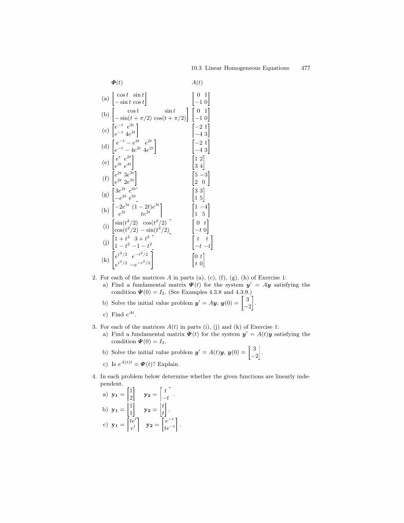
10.3 Linear Homogeneous Equations 477
Φ(t) A(t)
(a) cos t sin t− sin t cos t 0 1
−1 0(b) cos t sin t
− sin(t + π/2) cos(t + π/2) 0 1−1 0
(c) e−t e2t
e−t 4e2t −2 1−4 3
(d) e−t − e2t e2t
e−t − 4e2t 4e2t −2 1−4 3
(e) et e2t
e3t e4t 1 23 4
(f) e2t 3e3t
e2t 2e3t 5 −32 0
(g) 3e2t e6t
−e2t e6t 3 31 5
(h) −2e3t (1 − 2t)e3t
e3t te3t 1 −41 5
(i) sin(t2/2) cos(t2/2)cos(t2/2) − sin(t2/2) 0 t
−t 0(j) 1 + t2 3 + t2
1 − t2 −1 − t2 t t−t −t
(k) &et2/2 e−t2/2
et2/2 −e−t2/2' 0 tt 0
2. For each of the matrices A in parts (a), (c), (f), (g), (h) of Exercise 1:a) Find a fundamental matrix Ψ (t) for the system y′ = Ay satisfying the
condition Ψ (0) = I2. (See Examples 4.3.8 and 4.3.9.)
b) Solve the initial value problem y′ = Ay, y(0) = 3−2.
c) Find eAt.
3. For each of the matrices A(t) in parts (i), (j) and (k) of Exercise 1:a) Find a fundamental matrix Ψ (t) for the system y′ = A(t)y satisfying the
condition Ψ (0) = I2.
b) Solve the initial value problem y′ = A(t)y, y(0) = 3−2.
c) Is eA(t)t = Ψ (t)? Explain.
4. In each problem below determine whether the given functions are linearly inde-pendent.
a) y1 = 12 y2 = t−t .
b) y1 = 11 y2 = tt .
c) y1 = tet
et y2 = e−t
te−t .
478 10 Systems of Differential Equations
d) y1 = 1tt2 y2 = 01
t y3 = 001 .
10.4 Constant Coefficient Homogeneous Systems
In previous sections we studied some of the basic properties of the homoge-neous linear system of differential equations
y′ = A(t)y. (1)
In the case of a constant coefficient system, i.e., A(t) = A = a constant ma-trix, this analysis culminated in Theorem 13 which states that a fundamentalmatrix for y′ = Ay is the matrix exponential function eAt and the uniquesolution of the initial value problem y′ = Ay, y(0) = y0 is
y(t) = eAty0.
That is, the solution of the initial value problem is obtained by multiplyingthe fundamental matrix eAt by the initial value vector y0. The problem ofhow to compute eAt for a particular constant matrix A was not addressed,except for a few special cases where eAt could be computed directly from theseries definition of eAt. In this section we will show how to use the Laplacetransform to solve the constant coefficient homogeneous system y′ = Ay andin the process we will arrive at a Laplace transform formula for eAt.
As we have done previously, we will do our calculations in detail for the case
of a constant coefficient linear system where the coefficient matrix A =
[
a bc d
]
is a 2× 2 constant matrix so that Equation (1) becomes
y′1 = ay1 + by2
y′2 = cy1 + dy2.(2)
The calculations are easily extended to systems with more than 2 unknownfunctions. According to the existence and uniqueness theorem (Theorem 2)
there is a solution y(t) =
[
y1(t)y2(t)
]
for system (2), and we assume that the
functions y1(t) and y2(t) have Laplace transforms. From Chapter 3, we knowthat this is a relatively mild restriction on these functions, since, in particular,all functions of exponential growth have Laplace transforms. Our strategywill be to use the Laplace transform of the system (2) to determine what thesolution must be.
Let Y1(s) = L(y1) and Y2(s) = L(y2). Applying the Laplace transform toeach equation in system (2) and using the formulas from Table C.2 gives asystem of algebraic equations
10.4 Constant Coefficient Homogeneous Systems 479
sY1(s)− y1(0) = aY1(s) + bY2(s)
sY2(s)− y2(0) = cY1(s) + dY2(s).(3)
Letting Y =
[
Y1
Y2
]
, the system (3) can be written compactly in matrix form
assY (s)− y(0) = AY (s)
which is then easily rewritten as the matrix equation
(sI −A)Y (s) = y(0). (4)
If the matrix sI − A is invertible, then we may solve Equation (4) for Y (s),and then apply the inverse Laplace transform to the entries of Y (s) to findthe unknown functions y(t). But
sI −A =
[
s− a −b−c s− d
]
(5)
so p(s) = det(sI − A) = (s − a)(s − b) − bc = s2 − (a + d)s + (ad − bc) =s2 − Tr(A)s+ det(A). Hence p(s) is a nonzero polynomial function of degree2, so that the matrix sI − A is invertible as a matrix of rational functions,although one should note that for certain (the ≤ 2 roots of p(s)) values ofs the numerical matrix will not be invertible. For the purposes of Laplacetransforms, we are only interested in the inverse of sI − A as a matrix ofrational functions. Hence we may solve Equation (4) for Y (s) to get
Y (s) = (sI −A)−1y(0). (6)
Now
(sI −A)−1
=1
p(s)
[
s− d bc s− a
]
(7)
so let Z1(s) =1
p(s)
[
s− dc
]
and Z2(s) =1
p(s)
[
bs− a
]
be the first and second
columns of (sI −A)−1
:= Z(s), respectively. Since each entry of Z1(s) andZ2(s) is a rational function of s with denominator the quadratic polynomialp(s), the analysis of inverse Laplace transforms of rational functions of s withquadratic denominator from Section 6.4 applies to show that each entry of
z1(t) = L−1Z1(s) =
L−1
(
s− dp(s)
)
L−1
(
c
p(s)
)
and z2(t) = L−1Z2(s) =
L−1
(
b
p(s)
)
L−1
(
s− ap(s)
)
will be of the form
1. c1er1t + c2er2t if p(s) has distinct real roots r1 6= r2;
480 10 Systems of Differential Equations
2. c1ert + c2tert if p(s) has a double root r; or
3. c1eαt cosβt+ c2eαt sinβt if p(s) has complex roots α± iβ,
where c1 and c2 are appropriate constants. Equation (6) shows that
Y (s) = Z(s)y(0)
= y1(0)Z1(s) + y2(0)Z2(s), (8)
and by applying the inverse Laplace transform we conclude that the solutionto Equation (2) is
y(t) = y1(0)z1(t) + y2(0)z2(t). (9)
If we letz(t) =
[
z1(t) z2(t)]
= L−1(
(sI −A)−1)
, (10)
then Equation (9) for the solution y(t) of system (2) has a particularly niceand useful matrix formulation:
y(t) = z(t)y(0). (11)
Before analyzing Equation (11) further to extract theoretical conclusions,we will first see what the solutions look like in a few numerical examples.
Example 1. Find all solutions of the constant coefficient homogeneous lin-ear system:
y′1 = y2
y′2 = 4y1.(12)
I Solution. In this system the coefficient matrix is A =
[
0 14 0
]
. Thus sI −
A =
[
s −1−4 s
]
so that p(s) = det(sI −A) = s2 − 4 and
(sI −A)−1
=
s
s2 − 4
1
s2 − 4
4
s2 − 4
s
s2 − 4
. (13)
Since
1
s2 − 4=
1
4
(
1
s− 2− 1
s+ 2
)
ands
s2 − 4=
1
2
(
1
s− 2+
1
s+ 2
)
,
we conclude from our Laplace transform formulas (Table C.2) that the matrixz(t) of Equation (10) is
10.4 Constant Coefficient Homogeneous Systems 481
z(t) =
1
2
(
e2t + e−2t) 1
4
(
e2t − e−2t)
e2t − e−2t 1
2
(
e2t + e−2t)
. (14)
Hence, the solution of the system (12) is
y(t) =
1
2
(
e2t + e−2t) 1
4
(
e2t − e−2t)
e2t − e−2t 1
2
(
e2t + e−2t)
[
c1c2
]
=
1
2c1 +
1
4c2
c1 +1
2c2
e2t +
1
2c1 −
1
4c2
−c1 +1
2c2
e−2t,
(15)
where y(0) =
[
y1(0)y2(0)
]
=
[
c1c2
]
.
Let’s check that we have, indeed, found a solution to the system of differ-ential equations (2). From Equation (15) we see that
y1(t) =
(
1
2c1 +
1
4c2
)
e2t +
(
1
2c1 −
1
4c2
)
e−2t,
and
y2(t) =
(
c1 +1
2c2
)
e2t +
(
−c1 −1
2c2
)
e−2t.
Thus y′1(t) = y2(t) and y′2(t) = 4y1(t), which is what it means to be a solutionof system (12).
The solution to system (12) with initial conditions y1(0) = 1, y2(0) = 0 is
y1(t) =
1
2
1
e2t +
1
2
−1
e−2t
while the solution with initial conditions y1(0) = 0, y2(0) = 1 is
y2(t) =
1
4
1
2
e2t +
−1
4
1
2
e−2t.
The solution with initial conditions y1(0) = c1, y2(0) = c2 can then be written
y(t) = c1y1(t) + c2y2(t),
482 10 Systems of Differential Equations
that is, every solution y of system (12) is a linear combination of the two
particular solution y1 and y2. Note, in particular, that y3(t) =
[
12
]
e2t is a
solution (with c1 = 1, c2 = 2), while y4 =
[
1−2
]
e−2t is also a solution (with
c1 = 1, c2 = −2). The solutions y3(t) and y4(t) are notably simple solutionsin that each of these solutions is of the form
y(t) = veat (16)
where v ∈ R2 is a constant vector and a is a scalar. Note that
A
[
12
]
=
[
24
]
= 2
[
12
]
and A
[
1−2
]
=
[
−24
]
= −2
[
1−2
]
.
That is, the vectors v and scalars a such that y(t) = veat is a solution toy′ = Ay are related by the algebraic equation
Av = av. (17)
A vector-scalar pair (v, a) which satisfies Equation 17 is known as a eigenvector-eigenvalue pair for the matrix A. Finally, compare these two solutions y3(t)and y4(t) of the matrix differential equation y′ = Ay with the solution ofthe scalar differential equation y′ = ay, which we recall (see Section 2.2) isy(t) = veat where v = y(0) ∈ R is a scalar. In both cases one gets either ascalar or a vector multiplied by a pure exponential function eat. J
Example 2. Find all solutions of the linear homogeneous system
y′1 = y1 + y2
y′2 = −4y1 − 3y2.(18)
I Solution. For this system, the coefficient matrix is A =
[
1 1−4 −3
]
. We
will solve this equation by using Equation (11). Form the matrix
sI −A =
[
s− 1 −14 s+ 3
]
.
Then p(s) = det(sI −A) = (s− 1)(s+ 3) + 4 = (s+ 1)2, so that
(sI −A)−1 =1
(s+ 1)2
[
s+ 3 1−4 s− 1
]
=
1
s+ 1+
2
(s+ 1)21
(s+ 1)2
−4
(s+ 1)21
s+ 1− 2
(s+ 1)2
.
(19)
10.4 Constant Coefficient Homogeneous Systems 483
Thus the matrix z(t) from Equation (10) is, using the inverse Laplace formulasfrom Table C.2
z(t) = L−1(
(sI −A)−1)
=
[
e−t + 2te−t te−t
−4te−t e−t − 2te−t
]
.
The general solution to system (18) is therefore
y(t) = z(t)y(0) = c1
[
e−t + 2te−t
−4te−t
]
+ c2
[
te−1
e−t − 2te−t
]
. (20)
Taking c1 = 1 and c2 = −2 in this equation gives a solution
y1(t) =
[
e−t
−2e−t
]
=
[
1−2
]
e−t,
which is a solution of the form y(t) = veat where v =
[
1−2
]
is a constant
vector and a = −1 is a scalar. Note that (v, −1) is an eigenvector-eigenvaluepair for the matrix A (see Example 1). That is,
Av = A
[
1 1−1 −3
] [
1−2
]
=
[
−12
]
= (−1) ·[
1−2
]
.
J
Example 3. Find the solution of the linear homogeneous initial value prob-lem:
y′1 = y1 + 2y2
y′2 = −2y1 + y2, y1(0) = c1, y2(0) = c2. (21)
I Solution. For this system, the coefficient matrix is A =
[
1 2−2 1
]
. We will
solve this equation by using Equation (11), as was done for the previousexamples. Form the matrix
sI −A =
[
s− 1 −22 s− 1
]
.
Then p(s) = det(sI −A) = (s− 1)2) + 4, so that
(sI −A)−1 =1
(s− 1)2 + 4
[
s− 1 2−2 s− 1
]
=
s− 1
(s− 1)2 + 4
2
(s− 1)2 + 4
−2
(s− 1)2 + 4
s− 1
(s− 1)2 + 4
.
484 10 Systems of Differential Equations
Hence, using the inverse Laplace transform formulas from Table C.2, the ma-trix z(t) of Equation (10) is
z(t) = L−1(
(sI −A)−1)
=
[
et cos 2t et sin 2t−et sin 2t et cos 2t
]
,
and the solution of system (21) is
y(t) =
[
y1(t)y2(t)
]
=
[
c1et cos 2t+ c2e
t sin 2t−c1et sin 2t+ c2e
t cos 2t
]
.
J
Now we return briefly to the theoretical significance of Equation (11).According to the analysis leading to (11), the unique solution of the initialvalue problem
(∗) y′ = Ay, y(0) = y0,
where A is a 2× 2 constant matrix, is
y(t) = z(t)y(0) = z(t)y0,
wherez(t) = L−1
(
(sI −A)−1)
.
But according to Theorem 13, the unique solution of the initial value problem(*) is
y(t) = eAty0.
These two descriptions of y(t) give an equality of matrix functions
(∗∗) L−1(
(sI −A)−1)
y0 = z(t)y0 = eAty0
which holds for all choices of the constant vector y0. But if C is a 2×2 matrix
then Ce1 = C
[
10
]
is the first column of C and Ce2 = C
[
01
]
is the second
column of C (check this!). Thus, if B and C are two 2× 2 matrices such thatBei = Cei for i = 1, 2, then B = C (since column i of B = column i of C fori = 1, 2). Taking y0 = ei for i = 1, 2, and applying this observation to thematrices of (∗∗), we arrive at the following result:
Theorem 4. If A is a 2× 2 constant matrix, then
eAt = L−1(
(sI −A)−1)
. (22)
10.4 Constant Coefficient Homogeneous Systems 485
Example 5. From the calculations of L−1(
(sI −A)−1)
done in Examples
1, 2 and 3 this theorem gives the following values of eAt:
A eAt
[
0 14 0
]
1
2
(
e2t + e−2t) 1
4
(
e2t − e−2t)
e2t − e−2t 1
2
(
e2t + e−2t)
[
1 1−4 −3
] [
e−t + 2te−t te−t
−4te−t e−t − 2te−t
]
[
1 2−2 1
] [
et cos 2t et sin 2t−et sin 2t et cos 2t
]
While our derivation of the formula for eAt in Theorem 4 was done for 2×2matrices, the formula remains valid for arbitrary constant n× n matrices A,and moreover, once one can guess that there is a relationship between eAt and
L−1(
(sI −A)−1)
, it is a simple matter to verify it by computing the Laplace
transform of the matrix function eAt. This computation is, in fact, almost thesame as the computation of L(eat) in Example ??.
Theorem 6. If A is an n × n constant matrix (whose entries can be eitherreal numbers or complex numbers), then
eAt = L−1(
(sI −A)−1)
. (23)
Proof. Note that if B is an n× n invertible matrix (of constants), then
d
dt
(
B−1eBt)
= B−1 d
dteBt = B−1BeBt = eBt,
so that
(†)∫ t
1
eBτ dτ = B−1(eBt − I).
Note that this is just the matrix analog of the integration formula
∫ t
0
ebτ dτ = b−1(ebt − 1).
486 10 Systems of Differential Equations
Now just mimic the scalar calculation from Example ??, and note that formula(†) will be applied with B = A− sI, where, as usual, I will denote the n× nidentity matrix.
L(
eAt)
(s) =
∫ ∞
0
eAte−st dt
=
∫ ∞
0
eAte−stI dt
=
∫ ∞
0
e(A−sI)t dt
= limN→∞
∫ N
0
e(A−sI)t dt
= limN→∞
(A− sI)−1(
e(A−sI)N − I)
= (sI −A)−1.
The last equality is justified since limN→∞ e(A−sI)N = 0 if s is large enough.This fact, analogous to the fact that e(a−s)t converges to 0 as t→∞ provideds > a, will not be proved. ut
Example 7. Compute eAt for the matrix
A =
1 −3 3−3 1 33 −3 1
,
and using the calculation of eAt, solve the initial value problem y′ = Ay,
y(0) =
111
.
I Solution. According to Theorem 6, eAt = L−1(
(sI −A)−1)
, so we need
to begin by computing (sI −A)−1, which is most conveniently done (by hand)
by using the adjoint formula for a matrix inverse (see Corollary 8). Recallthat this formula says that if B is an n × n matrix with detB 6= 0, thenB−1 = (detB)−1[Cij ] where the term Cij is (−1)i+j times the determinantof the matrix obtained by deleting the jth row and ith column from B. Weapply this with B = sI −A. Start by calculating
p(s) = det(sI −A) = det
s− 1 3 −33 s− 1 −3−3 3 s− 1
= (s− 1)(s+ 2)(s− 4).
In particular, sI−A is invertible whenever p(s) 6= 0, i.e., whenever s 6= 1, −2,or 4. Then a tedious, but straightforward calculation, gives
10.4 Constant Coefficient Homogeneous Systems 487
(sI −A)−1 =1
p(s)
(s− 1)2 + 9 −3(s+ 2) 3(s− 4)−3(s− 4) (s− 1)2 − 9 3(s− 4)3(s+ 2) −3(s+ 2) (s− 1)2 − 9
=
(s− 1)2 + 9
p(s)
−3
(s− 1)(s+ 4)
3
(s− 1)(s+ 2)−3
(s− 1)(s+ 2)
1
s− 1
3
(s− 1)(s+ 2)3
(s− 1)(s− 4)
−3
(s− 1)(s− 4)
1
s− 1
=
− 1
s− 1+
1
s+ 2+
1
s− 4
1
s− 1− 1
s− 4
1
s+ 1− 1
s+ 2−1
s− 1+
1
s+ 2
1
s− 1
1
s+ 1− 1
s+ 2−1
s− 1+
1
s− 4
1
s− 1− 1
s− 4
1
s− 1
.
By applying the inverse Laplace transform to each function in the last matrixgives
eAt = L−1(
(sI −A)−1)
=
−et + e−2t + e4t et − e4t et − e−2t
−et + e−2t et et − e−2t
−et + e4t et − e4t et
.
Then the solution of the initial value problem is given by y(t) = eAt
111
=
111
et. J
Remark 8. Most of the examples of numerical systems which we have dis-cussed in this section are first order constant coefficient linear systems withtwo unknown functions, i.e. n = 2 in Definition 3. Nevertheless, the sameanalysis works for first order constant coefficient linear systems in any num-ber of unknown functions, i.e. arbitrary n. Specifically, Equations (6) and (11)apply to give the Laplace transform Y (s) and the solution function y(t) forthe constant coefficient homogeneous linear system
y′ = Ay
where A is an n× n constant matrix. The practical difficulty in carrying outthis program is in calculating (sI − A)−1. This can be done by programslike Mathematica, MatLab, or Maple if n is not too large. But even if thecalculations of specific entries in the matrix (sI − A)−1 are difficult, one canextract useful theoretical information concerning the nature of the solutionsof y′ = Ay + q(t) from the formulas like Equation (11) and from theoreticalalgebraic descriptions of the inverse matrix (sI −A)−1.
488 10 Systems of Differential Equations
Exercises
For each of the following matrices A, (a) find the matrix z(t) = L−1 (sI − A)−1from Equation (4.4.10) and (b) find the general solution of the homogeneous systemy′ = Ay. It will be useful to review the calculations in Examples 4.4.1 – 4.4.3.
1. −1 00 3 2. 0 2
−2 0 3. 2 10 2
4. −1 2−2 −1 5. 2 −1
3 −2 6. 3 −41 −1
7. 2 −51 −2 8. −1 −4
1 −1 9. 2 11 2
10. 5 2−8 −3 11. −1 0 3
0 2 00 0 1 12. 0 4 0
−1 0 01 4 −1
13. −2 2 10 −1 02 −2 −1 14. 0 1 1
1 1 −1−2 1 3 15. 3 1 −1
0 3 −10 0 3
10.5 Computing eAt
In this section we will present a variant of a technique due to Fulmer2 forcomputing the matrix exponential eAt. It is based on the knowledge of whattype of functions are included in the individual entries of eAt. This knowledgeis derived from our understanding of the Laplace transform table and thefundamental formula
eAt = L−1(
(sI −A)−1)
which was proved in Theorem 6.To get started, assume that A is an n × n constant matrix. The matrix
sI −A is known as the characteristic matrix of A and its determinant
p(s) := det(sI −A)
is known as the characteristic polynomial of A. The following are somebasic properties of sI−A and p(s) which are easily derived from the propertiesof determinants in Section 9.4.
1. The polynomial p(s) has degree n, when A is an n× n matrix.2. The characteristic matrix sI −A is invertible except when p(s) = 0.3. Since p(s) is a polynomial of degree n, it has at most n roots (exactly n if
multiplicity of roots and complex roots are considered). The roots of p(s)are called the eigenvalues of A.
2Edward P. Fulmer, Computation of the Matrix Exponential, American Mathe-
matical Monthly, 82 (1975) 156–159.
10.5 Computing eAt 489
4. The inverse of sI −A is given by the adjoint formula (Corollary 8)
(∗) (sI −A)−1
=1
p(s)[Cij(s)] =
[
Cij(s)
p(s)
]
where Cij(s) is (−1)i+j times the determinant of the matrix obtained fromsI−A by deleting the ith column and jth row. For example, if n = 2 thenwe get the formula
[
s− a −b−c s− d
]−1
=1
p(s)
[
s− d bc s− a
]
which we used in Section 10.4.5. The functions Cij(s) appearing in (∗) are polynomials of degree at mostn− 1. Therefore, the entries
pij(s) =Cij(s)
p(s)
of (sI−A)−1 are proper rational functions with denominator of degree n.6. Since
eAt = L−1(
(sI −A)−1)
=
[
L−1
(
Cij(s)
p(s)
)]
,
the form of the functions
hij(t) = L−1
(
Cij(s)
p(s)
)
,
which are the individual entries of the matrix exponential eAt, are com-pletely determined by the roots of p(s) and their multiplicities via theanalysis of inverse Laplace transforms of rational functions as describedin Section 3.3.
7. Suppose that r is an eigenvalue of A of multiplicity k. That is, r is a rootof the characteristic polynomial p(s) and (s − r)k divides p(s), but nohigher power of s− r divides p(s). We distinguish two cases:
Case 1: The eigenvalue r is real.In this case r will contribute a linear combination of the functions
(∗real) ert, tert, · · · , tk−1ert
to each hij .Case 2: The eigenvalue r = α+ iβ has nonzero imaginary part β 6= 0.
In this case r = α + iβ and its complex conjugate r = α − iβ willcontribute a linear combination of the functions
(∗Imag.)eαt cosβt, teαt cosβt, · · · , tk−1eαt cosβt
eαt sinβt, teαt sinβt, · · · , tk−1eαt sinβt
to each hij .
490 10 Systems of Differential Equations
8. The total number of functions listed in (∗real) and (∗Imag.) counting all
eigenvalues is n = deg p(s). If we let φ1, . . ., φn be these n functions, thenit follows from our analysis above, that each entry hij(t) can be writtenas a linear combination
(∗) hij(t) = mij1φ1(t) + · · ·+mijnφn(t)
of φ1, . . ., φn. We will define an n × n matrix Mk = [mijk] whose ijth
entry is the coefficient of φk(t) in the expansion of hij(t) in (∗). Then wehave a matrix equation expressing this linear combination relation:
(∗∗) eAt = [hij(t)] = M1φ1(t) + · · ·+Mnφ(t).
Example 1. As a specific example of the decomposion given by (∗∗), con-sider the matrix eAt from Example 7:
eAt =
−et + e−2t + e4t et − e4t et − e−2t
−et + e−2t et et − e−2t
−et + e4t et − e4t et
.
In this case (refer to Example 7 for details), p(s) = (s − 1)(s + 2)(s − 4) sothe eigenvalues are 1, −2 and 4 and the basic functions φi(t) are φ1(t) = et,φ2(t) = e−2t and φ3(t) = e4t. Then (∗∗) is the identity
eAt =
−1 1 1−1 1 1−1 1 1
et +
1 0 −11 0 −10 0 1
e−2t +
1 −1 00 0 01 −1 0
e4t,
where
M1 =
−1 1 1−1 1 1−1 1 1
, M2 =
1 0 −11 0 −10 0 1
and M3 =
1 −1 00 0 01 −1 0
.
With the notational preliminaries out of the way, we can give the variationon Fulmer’s algorithm for eAt.
Algorithm 2 (Fulmer’s method). The following procedure will computeeAt where A is a given n× n constant matrix.
1. Compute p(s) = det(sI −A).2. Find all roots and multiplicities of the roots of p(s).3. From the above observations we have
(‡) eAt = M1φ1(t) + · · ·+Mnφn(t),
where Mi i = 1, . . . , n are n×n matrices. We need to find these matrices.By taking derivatives we obtain a system of linear equations (with matrixcoefficients)
10.5 Computing eAt 491
eAt = M1φ1(t) + · · ·+Mnφn(t)
AeAt = M1φ′1(t) + · · ·+Mnφ
′n(t)
...
An−1eAt = M1φ(n−1)1 (t) + · · ·+Mnφ
(n−1)n (t).
Now we evaluate this system at t = 0 to obtain
I = M1φ1(0) + · · · + Mnφn(0)A = M1φ
′1(0) + · · · + Mnφ
′n(0)
. . . . . . . . . . . . . . . . . . . . . . . . . . . . . . . . . . . . . . . . . . . . . .
An−1 = M1φ(n−1)1 (0) + · · · + Mnφ
(n−1)n (0).
(1)
Let
W =
φ1(0) . . . φn(0)...
. . ....
φ(n−1)1 (0) . . . φ
(n−1)n (0)
Then W is a nonsingular n× n matrix; its determinant is just the Wron-skian evaluated at 0. So W has an inverse. The above system of equationscan now be written:
IA...
An−1
= W
M1
M2
...Mn
.
Therefore,
W−1
IA...
An−1
=
M1
M2
...Mn
.
Having solved for M1, . . . ,Mn we obtain eAt from (‡). ut
Remark 3. Note that this last equation implies that each matrix Mi is apolynomial in the matrix A since W−1 is a constant matrix. Specifically,Mi = pi(A) where
pi(s) = Rowi(W−1)
1s...
sn−1
.
Example 4. Solve y′ = Ay with initial condition y(0) =
[
12
]
, where A =[
2 −11 0
]
.
492 10 Systems of Differential Equations
I Solution. The characteristic polynomial is p(s) = (s − 1)2. Thus thereis only one eigenvalue r = 1 with multiplicity 2 so only case (∗real) occursand all of the entries hij(t) from eAt are linear combinations of et, tet. Thatis φ1(t) = et while φ2(t) = tet. Therefore, Equation (∗∗) is
eAt = Met +Ntet.
Differentiating we obtain
AeAt = Met +N(et + tet)
= (M +N)et +Ntet.
Now, evaluate each equation at t = 0 to obtain:
I = M
A = M +N.
Solving for M and N we get
M = I
N = A− I.
Thus,
eAt = Iet + (A− I)tet
=
[
1 00 1
]
et +
[
1 −11 −1
]
tet
=
[
et + tet −tet
tet et − tet
]
We now obtain
y(t) = eAty0 = eAt
[
12
]
=
[
et + tet −tet
tet et − tet
] [
12
]
=
[
et − tet
−tet + 2et
]
.
J
Example 5. Compute eAt where A =
1 − 12 0
1 1 −10 1
2 1
using Fulmer’s method.
10.5 Computing eAt 493
I Solution. The characteristic polynomial is p(s) = (s − 1)(s2 − 2s + 2).The eigenvalues of A are thus r = 1 and r = 1± i. From (∗real) and (∗Imag.)
each entry of eAt is a linear combination of
φ1(t) = et, φ2(t) = et sin t, and φ3(t) = et cos t.
ThereforeeAt = Met +Net sin t+ Pet cos t.
Differentiating twice and simplifying we get the system:
eAt = Met +Net sin t+ Pet cos t
AeAt = Met + (N − P )et sin t+ (N + P )et cos t
A2eAt = Met − 2Pet sin t+ 2Net cos t.
Now evaluating at t = 0 gives
I = M + P
A = M +N + P
A2 = M + 2N.
Solving gives
N = A− IM = A2 − 2A+ 2I
P = −A2 + 2A− I.
Since A2 =
12 −1 1
22 0 −212 1 1
2
, it follows that
N =
0 −12 0
1 0 −10 1
2 0
M =
12 0 1
20 0 012 0 1
2
and P =
12 0 −1
20 1 0−12 0 1
2
.
Hence,
eAt =
12 0 1
20 0 012 0 1
2
et +
0 −12 0
1 0 −10 1
2 0
et sin t+
12 0 −1
20 1 0−12 0 1
2
et cos t
=1
2
et + et cos t −et sin t et − et cos t2et sin t 2et cos t −2et sin t
et − et cos t et sin t et + et cos t
.
J
The technique of this section is convenient for giving an explicit formulafor the matrix exponential eAt when A is either a 2× 2 or 3× 3 matrix.

494 10 Systems of Differential Equations
eA for 2× 2 matrices.
Suppose that A is a 2 × 2 real matrix with characteristic polynomial p(s) =det(sI −A) = s2 + as+ b. We distinguish three cases.
1. p(s) = (s− r1)(s− r2) with r1 6= r2.Then the basic functions are φ1(t) = et1t and φ2(t) = er2t so that eAt =Mer1t +Ner2t. Equation (1) is then
I = M +N
A = r1M + r2N
which are easily solved to give
M =(A− r2I)r1 − r2
and N =(A− r1I)r2 − r1
.
Hence, if p(s) has distinct roots, then
eAt =(A− r2I)r1 − r2
er1t +(A− r1I)r2 − r1
er2t. (2)
2. p(s) = (s− r)2.In this case the basic functions are ert and tert so that
(∗) eAt = Mert +Ntert.
This time it is more convenient to work directly from (∗) rather than Equa-tion (1). Multiplying (∗) by e−rt and observing that eAte−rt = eAte−rtI =e(A−rI)t (because A commutes with rI), we get
M +Nt = e(A−rI)t
= I + (A− rI)t+1
2(A− rI)2t2 + · · · .
Comparing coefficients of t on both sides of the equation we conclude that
M = I, N = (A− rI) and (A− rI)n = 0 for all n ≥ 2.
Hence, if p(s) has a single root of multiplicity 2, then
eAt = (I + (A− rI)t) ert. (3)
10.5 Computing eAt 495
3. p(s) = (s−α)2 +β2 where β 6= 0, i.e., p(s) has a pair of complex conjugateroots α± β.In this case the basic functions are eαt cosβt and eαt sinβt so that
eAt = Meαt cosβt+Meαt sinβt.
Equation (1) is easily checked to be
I = M
A = αM + βN.
Solving for M and N then gives
eAt = Ieαt cosβt+(A− αI)
βeαt sinβt. (4)
eA for 3× 3 matrices.
Suppose that A is a 3 × 3 real matrix with characteristic polynomial p(s) =det(sI −A). As for 2× 2 matrices, we distinguish three cases.
1. p(s) = (s− r1)(s− r2)(s− r3) with r1. r2, and r3 distinct roots of p(s).This is similar to the first case done above. The basic functions are er1t,er2t, and er3t so that
eAt = Mer1t +Ner2t + Per3t
and the system of equations (1) is
I = M + N + PA = r1M+ r2N+ r3PA2 = r21M+ r22N+ r23P.
(5)
We will use a very convenient trick for solving this system of equations.Suppose that q(s) = s2 + as + b is any quadratic polynomial. Then insystem (5), multiply the first equation by b, the second equation by a,and then add the three resulting equations together. You will get
A2 + aA+ bI = q(A) = q(r1)M + q(r2)N + q(r3)P.
Suppose that we can choose q(s) so that q(r2) = 0 and q(r3) = 0. Since aquadratic can only have 2 roots, we will have q(r1) 6= 0 and hence
M =q(A)
q(r1).
496 10 Systems of Differential Equations
But it is easy to find the required q(s), namely, use q(s) = (s−r2)(s−r3).This polynomial certainly has roots r2 and r3. Thus, we find
M =(A− r2I)(A− r3I)(r1 − r2)(r1 − r3)
.
Similarly, we can find N by using q(s) = (s− r1)(s− r3) and P by usingq(s) = (s− r1)(s− r2). Hence, we find the following expression for eAt:
eAt =(A − r2I)(A− r3I)
(r1 − r2)(r1 − r3)er1t +
(A − r1I)(A − r3I)
(r2 − r1)(r2 − r3)er2t +
(A − r1I)(A − r2I)
(r3 − r1)(r3 − r2)er3t.
(6)
2. p(s) = (s− r)3, i.e, there is a single eigenvalue of multiplicity 3.In this case the basic functions are ert, tert, and t2ert so that
eAt = Mert +Ntert + Pt2ert.
As for the case of 2× 2 matrices, multiply by e−rt to get
M +Nt+ Pt2 = eAte−rt = e(A−rI)t
= I + (A− rI)t+1
2(A− rI)2t2 +
1
3!(A− rI)3t3 + · · · .
Comparing powers of t on both sides of the equation gives
M = I, N = (A− rI), P = (A−rI)2
2 and (A− rI)n = 0 if n ≥ 3.
Hence,
eAt =
(
I + (A− rI)t +1
2(A− rI)2t2
)
ert. (7)
3. p(s) = (s− r1)2(s− r2) where r1 6= r2. That is, A has one eigenvalue withmultiplicity 2 and another with multiplicity 1.The derivation is similar to that of the case p(s) = (s−r)3. We will simplyrecord the result:
eAt = I − (A − r1I)2
(r2 − r1)2 er1t + (A − r1I) − (A − r1I)2
r2 − r1 ter1t +(A − r1I)2
(r2 − r1)2er2t.
(8)
10.6 Nonhomogeneous Linear Systems 497
10.6 Nonhomogeneous Linear Systems
This section will be concerned with the nonhomogeneous linear equation
(∗) y′ = A(t)y + q(t),
where A(t) and q(t) are matrix functions defined on an interval J in R. Thestrategy will be analogous to that of Section 6.6 in that we will assume thatwe have a fundamental matrix Φ(t) =
[
ϕ1(t) · · · ϕn(t)]
of solutions of theassociated homogeneous system
(∗h) y′ = A(t)y
and we will then use this fundamental matrix Φ(t) to find a solution yp(t) of(∗) by the method of variation of parameters. Suppose that y1(t) and y2(t)are two solutions of the nonhomogeneous system (∗). Then
(y1−y2)′(t) = y′1(t)−y′2(t) = (A(t)y1(t)+q(t))−(A(t)y2(t)+q(t)) = A(t)(y1(t)−y2(t))
so that y1(t)−y2(t) is a solution of the associated homogeneous system (∗h).Since Φ(t) is a fundamental matrix of (∗h), this means that
y1(t)− y2(t) = Φ(t)c = c1ϕ1(t) + · · ·+ cnϕn(t)
for some constant matrix
c =
c1...cn
.
Thus it follows that if we can find one solution, which we will call yp(t), thenall other solutions are determined by the equation
y(t) = yp(t) +Φ(t)c = yp(t) + yh(t)
where yh(t) = Φ(t)c (c an arbitrary constant vector) is the solution of theassociated homogeneous equation (∗h). This is frequently expressed by themnemonic:
ygen(t) = yp(t) + yh(t), (1)
or in words: The general solution of a nonhomogeneous equation is the sum ofa particular solution and the general solution of the associated homogeneousequation. The strategy for finding a particular solution of (∗), assuming thatwe already know yh(t) = Φ(t)c, is to replace the constant vector c with anunknown vector function
498 10 Systems of Differential Equations
v(t) =
v1(t)...
vn(t)
.
That is, we will try to choose v(t) so that the vector function
(†) y(t) = Φ(t)v(t) = v1(t)ϕ1(t) + · · ·+ vn(t)ϕn(t)
is a solution of (∗). Differentiating y(t) gives y′(t) = Φ′(t)v(t) + Φ(t)v′(t),and substituting this expression for y′(t) into (∗) gives
Φ′(t)v(t) +Φ(t)v′(t) = y′(t) = A(t)y(t) + q(t) = A(t)Φ(t)v(t) + q(t).
But Φ′(t) = A(t)Φ(t) (since Φ(t) is a fundamental matrix for (∗h)) soΦ′(t)v(t) = A(t)Φ(t)v(t) cancels from both sides of the equation to give
Φ(t)v′(t) = q(t).
Since Φ(t) is a fundamental matrix Theorem 4 implies that Φ(t)−1 exists, andwe arrive at an equation
(‡) v′(t) = Φ(t)−1q(t)
for v′(t). Given an initial point t0 ∈ J , we can then integrate (‡) to get
v(t)− v(t0) =
∫ t
t0
Φ(u)−1q(u) du,
and multiplying by Φ(t) gives
y(t)−Φ(t)v(t0) = Φ(t)
∫ t
t0
Φ(u)−1q(u) du.
But if y(t0) = y0, then y0 = y(t0) = Φ(t0)v(t0), and hence v(t0) =Φ(t0)
−1y0. Substituting this expression in the above equation, we arrive atthe following result, which we formally record as a theorem.
Theorem 1. Suppose that A(t) and q(t) are continuous on an interval J andt0 ∈ J . If Φ(t) is a fundamental matrix for the homogeneous system y′ =A(t)y then the unique solution of the nonhomogeneous initial value problem
y′ = A(t)y + q(t), y(t0) = y0
is
y(t) = Φ(t) (Φ(t0))−1y0 +Φ(t)
∫ t
t0
Φ(u)−1q(u) du. (2)
10.6 Nonhomogeneous Linear Systems 499
Remark 2. The procedure described above is known as variation of para-meters for nonhomogeneous systems. It is completely analogous to thetechnique of variation of parameters previously studied for a single secondorder linear nonhomogeneous differential equation. See Section 6.6.
Remark 3. How does the solution of y′ = A(t)y+q(t) expressed by Equation(2) correlate to the general mnemonic expressed in Equation (1)? If we let theinitial condition y0 vary over all possible vectors in Rn, then yh(t) is thefirst part of the expression on the right of Equation (2). That is yh(t) =
Φ(t) (Φ(t0))−1y0. The second part of the expression on the right of Equation
(2) is the particular solution of y′ = A(t)y+q(t) corresponding to the specificinitial condition y(t0) = 0. Thus, in the language of (1)
yp = Φ(t)
∫ t
t0
Φ(u)−1q(u) du.
Finally, ygen(t) is just the function y(t), and the fact that it is the generalsolution is just the observation that the initial vector y0 is allowed to bearbitrary.
Example 4. Solve the initial value problem
y′ =
[
0 12 1
]
y +
[
0−et
]
, y(0) =
[
1−1
]
. (3)
I Solution. From Example 5 we have that
Φ(t) =
[
e2t e−t
2e2t −e−t
]
is a fundamental matrix for the homogeneous system y′ =
[
0 12 1
]
y, which is
the associated homogeneous system y′ = Ay for the nonhomogeneous system(3). Then detΦ(t) = −3et and
Φ(t)−1 =1
−3et
[
−e−t −e−t
−2e2t e2t
]
=1
3
[
e−2t e−2t
2et −et
]
.
Then
Φ(0)−1
[
1−1
]
=1
3
[
1 12 −1
] [
1−1
]
=
[
01
]
,
and hence
Φ(t)Φ(0)−1
[
1−1
]
=
[
e2t e−t
2e2t −e−t
] [
01
]
=
[
e−t
−e−t
]
.
which is the first part of y(t) in Equation (2). Now compute the second halfof Equation (2):
500 10 Systems of Differential Equations
Φ(t)
∫ t
t0
Φ(u)−1q(u) du =
[
e2t e−t
2e2t −e−t
]∫ t
0
1
3
[
e−2u e−2u
2eu −eu
] [
0−eu
]
du
=
[
e2t e−t
2e2t −e−t
]∫ t
0
1
3
[
−e−u
e2u
]
du
=
[
e2t e−t
2e2t −e−t
]
13 (e−t − 1)
16 (e2t − 1)
=
13 (et − e2t) + 1
6 (et − e−t)
23 (et − e2t)− 1
6 (et − e−t)
=
12e
t − 13e
2t − 16e
−t
12e
t − 23e
2t + 16e
−t
.
Putting together the two parts which make up y(t) in Equation (2) we get
y(t) =
[
e−t
−e−t
]
+
12e
t − 13e
2t − 16e
−t
12e
t − 23e
2t + 16e
−t
.
We will leave it as an exercise to check our work by substituting the aboveexpression for y(t) back into the system (3) to see that we have in fact foundthe solution. J
If the linear system y′ = Ay + q(t) is constant coefficient, then a funda-mental matrix for the associated homogeneous system is Φ(t) = eAt. Since(eAt)−1 = e−At, it follows that eAt(eAt0)−1 = eA(t−t0) and hence Theorem 1has the following form in this situation.
Theorem 5. Suppose that A is a constant matrix and q(t) is a continuousvector function on an interval J and t0 ∈ J . Then the unique solution of thenonhomogeneous initial value problem
y′ = Ay + q(t), y(t0) = y0
is
y(t) = eA(t−t0)y0 + eAt
∫ t
t0
e−Auq(u) du. (4)
You should compare the statement of this theorem with the solution ofthe first order linear initial value problem as expressed in Corollary 9.
Example 6. Solve the initial value problem
y′ =
[
−1 1−4 3
]
y +
[
et
2et
]
, y(0) =
[
10
]
.
10.6 Nonhomogeneous Linear Systems 501
I Solution. In this example, A =
[
−1 1−4 3
]
, q(t) =
[
et
2et
]
, t0 = 0, and y(0) =[
10
]
. Since the characteristic polynomial of A is p(s) = det(sI−A) = (s−1)2,
the fundamental matrix eAt can be computed from Equation (3):
eAt = (I + (A− I)t)et
=
[
1− 2t t−4t 1 + 2t
]
et.
Since e−At = eA·(−t), we can compute e−At by simply replacing t by −t in theformula for eAt:
e−At =
[
1 + 2t −t4t 1− 2t
]
e−t.
Then applying Equation (4) give
y(t) = eAty0 + eAt
∫ t
0
e−Auq(u) du
=
[
1− 2t t−4t 1 + 2t
]
et
[
10
]
+
[
1− 2t t−4t 1 + 2t
]
et
∫ t
0
[
1 + 2u −u4u 1− 2u
]
e−u
[
eu
2eu
]
du
=
[
(1− 2t)et
−4tet
]
+
[
1− 2t t−4t 1 + 2t
]
et
∫ t
0
[
12
]
du
=
[
(1− 2t)et
−4tet
]
+
[
1− 2t t−4t 1 + 2t
]
et
[
t2t
]
=
[
(1− 2t)et
−4tet
]
+
[
tet
2tet
]
.
J
If we take the initial point t0 = 0 in Theorem 5, then we can get a furtherrefinement of Equation (4) by observing that
eAt
∫ t
0
e−Auq(u) du =
∫ t
0
eA(t−u)q(u) du = eAt ∗ q(t)
where eAt ∗ q(t) means the matrix of functions obtained by a formal matrixmultiplication in which ordinary product of entries are replaced by the con-
volution product. For example, if B(t) =
[
h11(t) h12(t)h21(t) h22(t)
]
and q(t) =
[
q1(t)q2(t)
]
,
then by B(t) ∗ q(t) we mean the matrix
B(t)∗q(t) = (h11 ∗ q1)(t) + (h12 ∗ q2)(t)
(h21 ∗ q1)(t) + (h22 ∗ q2)(t) = t
0h11(t − u)q1(u) du +
t
0h12(t − u)q2(u) du t
0h21(t − u)q1(u) du +
t
0h22(t − u)q2(u) du .
With this observation we can give the following formulation of Theorem 5in terms of the convolution product.
502 10 Systems of Differential Equations
Theorem 7. Suppose that A is a constant matrix and q(t) is a continuousvector function on an interval J and 0 ∈ J . Then the unique solution of thenonhomogeneous initial value problem
y′ = Ay + q(t), y(t0) = y0
is
y(t) = eAty0 + eAt ∗ q(t). (5)
Remark 8. For low dimensional examples, the utility of this result is greatlyenhanced by the use of the explicit formulas (2) – (8) from the previous sectionand the table of convolution products (Table C.3).
Example 9. Solve the following constant coefficient non-homogeneous lin-ear system:
y′1 = y2 + e3t
y′2 = 4y1 + et.(6)
I Solution. In this system the coefficient matrix is A =
[
0 14 0
]
and q(t) =[
e3t
et
]
. The associated homogeneous equation y′ = Ay has already been stud-
ied in Example 1 where we found that a fundamental matrix is
z(t) =
1
2
(
e2t + e−2t) 1
4
(
e2t − e−2t)
e2t − e−2t 1
2
(
e2t + e−2t)
. (7)
Since, z(0) =
[
1 00 1
]
it follows that z(t) = eAt. If we write eAt in terms of its
columns, so that eAt =[
z1(t) z2(t)]
then we conclude that a solution of theinitial value problem
y′ = Ay + q(t), y(0) = 0
is given by
10.6 Nonhomogeneous Linear Systems 503
yp(t) = eAt ∗ q(t)= z1(t) ∗ q1(t) + z2(t) ∗ q2(t)= z1 ∗ e3t + z2 ∗ et
=
[
12
(
e2t + e−2t)
e2t − e−2t
]
∗ e3t +
[
14
(
e2t − e−2t)
12
(
e2t + e−2t)
]
∗ et
=
[
12
(
e3t − e2t + 15
(
e3t − e−2t))
e3t − e2t − 15
(
e3t − e−2t)
]
+
[
14
(
e2t − et − 13
(
et − e−2t))
12
(
e2t − et + 13
(
e3t − e−2t))
]
=
[
35e
3t − 12e
2t − 110e
−2t
45e
3t − e2t + 15e
−2t
]
+
[
14e
2t + 112e
−2t − 13e
t
12e
2t − 16e
−2t − 13e
t
]
=
[
35e
3t − 13e
t − 14e
2t − 160e
−2t
45e
3t − 13e
t − 12e
2t + 130e
−2t
]
.
The general solution to (6) is then obtained by taking yp(t) and adding
to it the general solution yh(t) = eAt
[
c1c2
]
of the associated homogeneous
equation. Hence,
ygen =
[
12 c1 + 1
4c2c1 + 1
2c2
]
e2t +
[
12c1 − 1
4c2−c1 + 1
2 c2
]
e−2t +
[
35e
3t − 13e
t − 14e
2t − 160e
−2t
45e
3t − 13e
t − 12e
2t + 130e
−2t
]
.
J
Exercises
In part (a) of each exercise in Section 4.4, you were asked to find eAt for the givenmatrix A. Using your answer to that exercise, solve the nonhomogeneous equation
y′ = Ay + q(t), y(0) = 0,
where A is the matrix in the corresponding exercise in Section 4.4 and q(t) is thefollowing matrix function. (Hint: Theorem 4.6.5 and Example 4.6.7 should proveparticularly useful to study for these exercises.)
1. q(t) = e−t
2et 2. q(t) = 0cos t 3. q(t) = t1
5. q(t) = et
e−t 7. q(t) = 0sin t 11. q(t) = et
e2t
e−t

A
Complex Numbers
A.1 Complex Numbers
The history of numbers starts in the stone age, about 30,000 years ago. Longbefore humans could read or write, a caveman who counted the deer he killedby a series of notches carved into a bone, introduced mankind to the naturalcounting numbers 1, 2, 3, 4, · · · . To be able to describe quantities and theirrelations among each other, the first human civilizations expanded the numbersystem first to rational numbers (integers and fractions) and then to realnumbers (rational numbers and irrational numbers like
√2 and π). Finally in
1545, to be able to tackle more advanced computational problems in his bookabout The Great Art (Ars Magna), Girolamo Cardano brought the complexnumbers (real numbers and “imaginary” numbers like
√−1) into existence.
Unfortunately, 450 years later and after changing the whole of mathematicsforever, complex numbers are still greeted by the general public with suspicionand confusion.
The problem is that most folks still think of numbers as entities that areused solely to describe quantities. This works reasonably well if one restrictsthe number universe to the real numbers, but fails miserably if one considerscomplex numbers: no one will ever catch
√−1 pounds of crawfish, not even a
mathematician.In mathematics, numbers are used to do computations, and it is a matter
of fact that nowadays almost all serious computations in mathematics requiresomewhere along the line the use of the largest possible number system givento mankind: the complex numbers. Although complex numbers are uselessto describe the weight of your catch of the day, they are indispensable if,for example, you want to make a sound mathematical prediction about thebehavior of any biological, chemical, or physical system in time.
Since the ancient Greeks, the algebraic concept of a real number is asso-ciated with the geometric concept of a point on a line (the number line), andthese two concepts are still used as synonyms. Similarly, complex numberscan be given a simple, concrete, geometric interpretation as points in a plane;
506 A Complex Numbers
i.e., any complex number z corresponds to a point in the plane (the numberplane) and can be represented in Cartesian coordinates as z = (x, y), wherex and y are real numbers.
We know from Calculus II that every point z = (x, y) in the plane can bedescribed also in polar coordinates as z = [α, r], where r = |z| =
√
x2 + y2
denotes the radius (length, modulus, norm, absolute value, distanceto the origin) of the point z, and where α = arg(z) is the angle (in radians)between the positive x-axis and the line joining 0 and z. Note that α can bedetermined by the equation tanα = y/x, when x 6= 0, and knowledge of whichquadrant the number z is in. Be aware that α is not unique; adding 2πk to αgives another angle (argument) for z.
We identify the real numbers with the x-axis in the plane; i.e., a realnumber x is identified with the point (x, 0) of the plane, and vice versa. Thus,the real numbers are a subset of the complex numbers. As pointed out above,in mathematics the defining property of numbers is not that they describequantities, but that we can do computations with them; i.e., we should beable to add and multiply them. The addition and multiplication of points inthe plane are defined in such a way that
(a) they coincide on the x-axis (real numbers) with the usual addition andmultiplication of real numbers, and
(b) all rules of algebra for real numbers (points on the x-axis) extend to com-plex numbers (points in the plane).
Addition: we add complex numbers coordinate-wise in Cartesian coordi-nates. That is, if z1 = (x1, y1) and z2 = (x2, y2), then
z1 + z2 = (x1, y1) + (x2, y2) := (x1 + x2, y1 + y2).
Multiplication: we multiply complex numbers in polar coordinates byadding their angles α and multiplying their radii r (in polar coordinates).That is, if z1 = [α1, r1] and z2 = [α2, r2], then
z1z2 := [α1 + α2, r1r2].
The definition of multiplication of points in the plane is an extension of thefamiliar rule for multiplication of signed real numbers: plus times plus is plus,minus times minus is plus, plus times minus is minus. To see this, we identifythe real numbers 2 and −3 with the complex numbers z1 = (2, 0) = [0, 2] andz2 = (−3, 0) = [π, 3]. Then
z1z2 = [0 + π, 2 · 3] = [π, 6] = (−6, 0) = −6
z22 = [π, 3][π, 3] = [π + π, 3 · 3] = [2π, 9] = (0, 9) = 9,
which is not at all surprising since we all know that 2·−3 = −6, and (−3)2 = 9.What this illustrates is part (a); namely, the arithmetic of real numbers is the
A.1 Complex Numbers 507
same whether considered in their own right, or considered as a subset of thecomplex numbers.
To demonstrate the multiplication of complex numbers (points in theplane) which are not real (not on the x-axis), consider z1 = (1, 1) = [π
4 ,√
2]
and z2 = (1,−1) = [−π4 ,√
2]. Then
z1z2 = [π
4− π
4,√
2 ·√
2] = [0, 2] = (2, 0) = 2.
If one defines multiplication of points in the plane as above, the pointi := (0, 1) = [π
2 , 1] has the property that
i2 = [π
2+π
2, 1 · 1] = [π, 1] = (−1, 0) = −1.
Thus, one defines √−1 := i = (0, 1).
Notice that√−1 is not on the x-axis and is therefore not a real number.
Employing i and identifying the point (1, 0) with the real number 1, one cannow write a complex number z = (x, y) in the standard algebraic formz = x+ iy; i.e.,
z = (x, y) = (x, 0) + (0, y) = x(1, 0) + (0, 1)y = x+ iy.
If z = (x, y) = x+ iy, then the real number x := Re z is called the real partand the real number y := Im z is called the imaginary part of z (which isone of the worst misnomers in the history of science since there is absolutelynothing imaginary about y).
The basic rules of algebra carry over to complex numbers if we simplyremember the identity i2 = −1. In particular, if z1 = x1+iy1 and z2 = x2+iy2,then
z1z2 = (x1 + iy1)(x2 + iy2) = x1x2 + iy1x2 + x1iy2 + iy1iy2
= (x1x2 − y1y2) + i(x1y2 + x2y1) = (x1x2 − y1y2, x1y2 + x2y1).
This algebraic rule is often easier to use than the geometric definition ofmultiplication given above. For example, if z1 = (1, 1) = 1 + i and z2 =(1,−1) = 1 − i, then the computation z1z2 = (1 + i)(1 − i) = 1 − i2 = 2 ismore familiar than the one given above using the polar coordinates of z1 andz2.
The formula for division of two complex numbers (points in the plane)is less obvious, and is most conveniently expressed in terms of the complexconjugate z := (x,−y) = x − iy of a complex number z = (x, y) = x + iy.Note that z + w = z + w, zw = z w, and
|z|2 = x2 + y2 = zz, Re z =z + z
2and Im z =
z − z2i
.
508 A Complex Numbers
Using complex conjugates, we divide complex numbers using the formula
z
w=z
w· ww
=zw
|w|2 .
As an example we divide the complex number z = (1, 1) = 1 + i byw = (3,−1) = 3− i. Then
z
w=
1 + i
3− i =(1 + i)(3 + i)
(3− i)(3 + i)=
2 + 4i
10=
1
5+
2
5i = (
1
5,2
5).
Let z = (x, y) be a complex number with polar coordinates z = [α, r].Then |z| = r =
√
x2 + y2, Re z = x = |z| cosα, Im z = y = |z| sinα, andtanα = y/x. Thus we obtain the following exponential form of the complexnumber z; i.e.,
z = [α, r] = (x, y) = |z|(cosα, sinα) = |z|(cosα+ i sinα) = |z|eiα,
where the last identity requires Euler’s formula relating the complex exponen-tial and trigonometric functions. The most natural means of understandingthe validity of Euler’s formula is via the power series expansions of ex, sinx,and cosx, which were studied in calculus. Recall that the exponential functionex has a power series expansion
ex =∞∑
n=0
xn
n!
which converges for all x ∈ R. This infinite series makes perfectly good senseif x is replaced by any complex number z, and moreover, it can be shownthat the resulting series converges for all z ∈ C. Thus, we define the complexexponential function by means of the convergent series
ez :=∞∑
n=0
zn
n!. (1)
It can be shown that this function ez satisfies the expected functional equation,that is
ez1+z2 = ez1ez2 .
Since e0 = 1, it follows that1
ez= e−z. Euler’s formula will be obtained by
taking z = it in Definition 1; i.e.,
eit =
∞∑
n=0
(it)n
n!= 1 + it− t2
2!− i t
3
3!+t4
4!+ i
t5
5!− · · ·
= (1− t2
2!+t4
4!− · · · ) + i(t− t3
3!+t5
5!− · · · ) = cos t+ i sin t = (cos t, sin t),
where one has to know that the two series following the last equality are theTaylor series expansions for cos t and sin t, respectively. Thus we have provedEuler’s formula, which we formally state as a theorem.

A.1 Complex Numbers 509
Theorem 1 (Euler’s Formula). For all t ∈ R we have
eit = cos t+ i sin t = (cos t, sin t) = [t, 1]. ut
Example 2. Write z = −1 + i in exponential form.
I Solution. Note that z = (−1, 1) so that x = −1, y = 1, r = |z| =√
(−1)2 + 12 =√
2, and tanα = y/x = −1. Thus, α = 3π4 or α = 7π
4 . But z isin the 2nd quadrant, so α = 3π
4 . Thus the polar coordinates of z are [ 3π4 ,√
2]
and the exponential form of z is√
2ei 3π4 . J
Example 3. Write z = 2eπi6 in Cartesian form.
I Solution.
z = 2(cosπ
6+ i sin
π
6) = 2
(√3
2+ i
1
2
)
=√
3 + i = (√
3, 1).
J
Using the exponential form of a complex number gives yet another de-scription of the multiplication of two complex numbers. Suppose that z1 andz2 are given in exponential form, that is, z1 = r1e
iα1 and z2 = r2eiα2 . Then
z1z2 = (r1eiα1)(r2e
iα2) = (r1r2)ei(α1+α2).
Of course, this is nothing more than a reiteration of the definition of mul-tiplication of complex numbers; i.e., if z1 = [α1, r1] and z2 = [α2, r2], thenz1z2 := [α1 + α2, r1r2].
Example 4. Find z =√i. That is, find all z such that z2 = i.
I Solution. Observe that i = (0, 1) = [π/2, 1] = eπ2 i. Hence, if z = ei π
4 thenz2 = (ei π
4 )2 = ei π2 = i so that
z = cosπ
4+ i sin
π
4=
√2
2+ i
√2
2=
√2
2(1 + i).
Also note that i = e(π2 +2π)i so that w = e(
π4 +π)i = e
π4 eπi = −eπ
4 = −z isanother square root of i. J
Example 5. Find all complex solutions to the equation z3 = 1.
I Solution. Note that 1 = e2πki for any integer k. Thus the cube roots of1 are obtained by dividing the possible arguments of 1 by 3 since raising acomplex number to the third power multiplies the argument by 3 (and alsocubes the modulus). Thus the possible cube roots of 1 are 1, ω = e
2π3 i =
− 12 +
√3
2 i and ω2 = e4π3 i = − 1
2 −√
32 . J
510 A Complex Numbers
We will conclude this section by summarizing some of the properties of thecomplex exponential function. The proofs are straight forward calculationsbased on Euler’s formula and are left to the reader.
Theorem 6. Let z = x+ iy. Then
1. ez = ex+iy = ex cos y + iex sin y. That is Re ez = ex cos y and Im ez =ex sin y.
2. |ez| = ex. That is, the modulus of ez is the exponential of the real part ofz.
3. cos y =eiy + e−iy
2
4. sin y =eiy − e−iy
2iut
Example 7. Compute the real and imaginary parts of the complex function
z(t) = (2 + 3i)ei 5t2 .
I Solution. Since z(t) = (2 + 3i)(cos 5t2 + i sin 5t
2 ) = (2 cos 5t2 − 3 sin 5t
2 ) +(3 cos 5t
2 + 2 sin 5t2 )i, it follows that Re z(t) = 2 cos 5t
2 − 3 sin 5t2 and Im z(t) =
3 cos 5t2 + 2 sin 5t
2 . J
Exercises
1. Let z = (1, 1) and w = (−1, 1). Find z · w, zw
, wz, z2,
√z and z11 using
(a) the polar coordinates,(b) the standard forms x + iy,(c) the exponential forms.
2. Find(a) (1+2i)(3+4i) (b) (1+2i)2 (c)
1
2 + 3i(d)
1
(2 − 3i)(2 + 4i)(e)
4 − 2i
2 + i.
3. Solve each of the following equations for z and check your result.
(a) (2 + 3i)z + 2 = i (b)z − 1
z − i=
2
3(c)
2 + i
z+ 1 = 2 + i (d)
ez = −1.
4. Find the modulus of each of the following complex numbers.
a) 4 + 3i (b) (2 + i)2 (c)13
5 + 12i(d)
1 + 2it − t2
1 + t2where t ∈ R.
5. Find all complex numbers z such that |z−1| = |z−2|. What does this equationmean geometrically?
6. Determine the region in the complex plane C described by the inequality
|z − 1| + |z − 3| < 4.
Give a geometric description of the region.
A.1 Complex Numbers 511
7. Compute: (a)√
2 + 2i (b)√
3 + 4i
8. Write each of the following complex numbers in exponential form.
a) 3 + 4i (b) 3 − 4i (c) (3 + 4i)2 (d)1
3 + 4i(e) −5 (f) 3i
9. Find the real and imaginary parts of each of the following functions.a) (2 + 3i)e(−1+i)t (b) ie2it+π (c) e(2+3i)te(−3−i)t
10. a) Find the value of the sum
1 + ez + e2z + · · · + e(n−1)z.
Hint: Compare the sum to a finite geometric series.b) Compute sin( 2π
n) + sin( 4π
n) + · · · + sin( (n−1)π
n)
11. Find all of the cube roots of 8i. That is, find all solutions to the equation z3 = 8i.
12. By multiplying out eiθeiφ and comparing it to ei(θ+φ), rederive the additionformulas for the cosine and sine functions.

B
Selected Answers
Chapter 1
Section 1.1
1. (a) 1 (b) 2 (c) 1 (d) 2 (e) 2 (f) 4 (g) 1 (h) 32. y1(t) and y3(t) are solutions. 3. y1(t) and y4(t) are solutions.4. y1(t), y2(t), and y3(t) are solutions. 5. y2(t) and y3(t) are solutions.12. y(t) = 1
2t2 + 3t + c 13. y(t) = 1
2e2t − t + c 14. y(t) = −e−t(t + 1) + c
15. y(t) = t + ln |t| + c 16. y(t) = t3
3+ t2
2+ c1t + c2 17. y(t) = − 2
3sin 3t + c1t + c2
18. y(t) = 2e3t − 4 19. y(t) = 3e−t + 3t − 3 20. y(t) = 1/(1 + et)21. y(t) = −18(t + 1)−1 22. y(t) = 1
2e2t − t + 7
223. y(t) = −e−t(t + 1)
24. y(t) = − 23
sin 3t + 4t + 125. 4yy′ + 3t = 0 26. 2yy′ = 3t2 + 2t27. y′ = 2y − 2t + 1 28. ty′ = 3y − t2
Section 1.2
1. From Example 1, the ball will hit the ground after T =
400/16 = 5 sec. Thespeed at this time is |y′(T )| = gT = 32 × 5 = 160 ft/sec.
2. According to Equation (4) the height at time t is y(t) = −(g/2)t2 + v0t + hand the maximum height is obtained when y′(t) = −gt + v0 = 0. That is, whent = v0/g. The ball will hit the ground when y(t) = 0, so solve the quadraticequation −(g/2)t2 + v0t + h = 0 to get t = (v0 +
v20 + 2gh)/g.
3. t1 ≈ .695 sec, t2 ≈ 4.407 sec.
4. From Equation (6) the gravitational constant is g = 2h/T 2 = 8 ft/sec2, so thesecond stone will have the height equation y(t) = −4t2 + 1000. When t = 5the height is y(5) = −4 × 25 + 1000 = 900 ft. It will hit the ground at timeT =
2h/g =
√250 ≈ 15.81 sec.
5. R′ = kR where k is a proportionality constant.
6. P ′ = kP where k is a proportionality constant.
514 B Selected Answers
7. P ′ = kP (M − P ) where k is a proportionality constant.
8. Recall that Newton’s Law of heating and cooling states: The change in the
temperature of an object is proportional to the difference between the temperature
of the object and the temperature of the surrounding medium. Thus, if T (t) isthe temperature of the beverage at time t and A is the temperature of thesurrounding medium then
T ′(t) = k(T − A),
for some proportionality constant k. In this case the surrounding medium isthe tub of ice, which has a temperature of A = 32 F, so that the differentialequation is T ′ = k(T − 32) with the initial value given by T (0) = 70 F. Theproportionality constant k cannot be determined from the given data.
9. In this case, the oven is the surrounding medium and has a constant temperatureof A = 350 F. Thus the differential equation, determined by Newton’s law ofcooling and heating, that describes the temperature of the turkey T (t) at timet is
T ′ = k(T − 350),
where k is a proportionality constant. The initial temperature of the turkey is40, so Equation (15) gives the solution of this differential equation as
T (t) = A + (T (0) − A)ekt = 350 + (40 − 350)ekt = 350 − 310ekt,
where the proportionality constant k is yet to be determined. To determine knote that we are given T (1) = 120. This implies 120 = T (1) = 350 − 310ek
and solving for k gives k = ln 2331
≈ −.298. To answer question (1), computeT (2) = 350 − 310e2k ≈ 179.35. To answer question (2), we want to find tso that T (t) = 250, i.e, solve 250 = T (t) = 350 − 310ekt. Solving this giveskt = ln 10
31so t ≈ 3.79 hours.
10. The initial temperature is T (0) = 180 and the ambient temperature is A = 70.Thus Equation (15) gives T (t) = A + (T (0) − A)ekt = 70 + 110ekt for thetemperature of the coffee at time t. The constant k is determined from thetemperature at a second time: T (3) = 140 = 70 + 110e3k so k ≈ −.1507. ThusT (t) = 70 + 110e−0.1507t . The temperature requested is T (5) = 121.8.
Section 1.3
Section 2.1
1. separable
2. not separable
3. separable
B Selected Answers 515
4. not separable
5. separable
6. not separable
7. separable
8. not separable
9. separable
12. y4 = 2t2 + c
13. 2y5 = 5(t+ 2)2 + c
14. y(t2 + c) = −2, y = 0
15. y =−3
t3 + c, y = 0
16. y = 1− c cos t, y = 1
17. y1−n =1− n1 +m
tm+1 + c, y = 0
18. y =4ce4t
1− ce4t, y = 4
19. y2 + 1 = ce2t
20. y = tan(t+ c)
21. t2 + y2 + 2 ln |t| = c
22. tan−1 t+ y − 2 ln |y + 1| = c, y = −1
23. y2 = et + c
24. y ln |c(1− t)| = 1
25. cet = y(t+ 2)2
26. y = 0
27. y = 0
28. y = x2ex
29. y = 4e−t2
30. y = sec−1(√
2t2)
516 B Selected Answers
31. y = 2√u2 + 1
Section 2.2
3. y(t) = te2t + 4e2t
4. y(t) = −1
4e−2t +
17
4e2t
5. y(t) =1
tet − e
t
6. y(t) =1
2t[e2t − e2]
7. y(t) = t+sin t cos t2 cos t + c sec t
8. y(t) = e−t2/2∫ t
0es2/2 ds+ e−t2/2
9. y(t) =t ln t
m+ 1− t
(m+ 1)2+ ct−m
10. y(t) = sin(t2)+c2t
11. y(t) = 1t+1 (−2 + ct)
12. y(t) = b/a+ ce−at
13. y(t) = 1
14. y(t) = t(t+ 1)2 + c(t+ 1)2
15. y(t) = −t− 1
2− 3
2t2
16. y(t) = te−at + ce−at
17. y(t) =1
a+ bebt + ce−at
18. y(t) =tn+1
n+ 1e−at + ce−at
19. y(t) = t+ccos t
20. y = 2 + ce−(ln t)2
21. y(t) = tnet + ctn
22. y(t) = (t− 1)e2t + (a+ 1)et
B Selected Answers 517
23. y(t) =t2
5− 9
5t−3
24. y(t) = 1t
[
1 +2(2a− 1)
t
]
25. y(t) = (10 − t) − 8(1 − t10 )4. Note that y(10) = 0, so the tank is empty
after 10 min.
26. (a) T = 45 min; (b) y(t) = 12 (10 + 2t) − 50(10 + 2t)−1 for 0 ≤ t ≤ 45
so y(45) = 50 − 12 = 49.5 lb. (c) limt→∞ y(t) = 50. Once the tank is
full, the inflow and outflow rates will be equal and the brine in the tankwill stabilize to the concentration of the incoming brine, i.e., .5 lb/gal.Since the tank holds 100 gal, the total amount present will approach.5× 100 = 50 lb.
27. If y(t) is the amount of salt present at time t (measured in pounds), theny(t) = 80e−.04t, and the concentration c(t) = .8e−.04t lb/gal.
28. a) Differential equation: P ′(t)+ (r/V )P (t) = rc. If P0 denotes the initialamount of pollutant in the lake, then P (t) = V c+ (P0 − V c)e−(r/V )t.The limiting concentration is c.
b) (i) t1/2 = (V/r) ln 2; (ii) t1/10 = (V/r) ln 10c) Lake Erie: t1/2 = 1.82 years, t1/10 = 6.05 years, Lake Ontario: t1/2 =
5.43 years, t1/10 = 18.06 years
29. a) 10 minutesb) 1600/3 grams
30. 1− e−1 grams/liter
Section 2.3
2. y1(t) = 1− t+t2
2
y2(t) = 1− t+ t2 − t3
6
y3(t) = 1− t+ t2 − t3
3+t4
4!
3. y1(t) =t2
2
y2(t) =t2
2+t5
20
y3(t) =t2
2+t5
20+
t8
160+
t11
44004. Unique solution5. Not guaranteed unique6. Unique solution
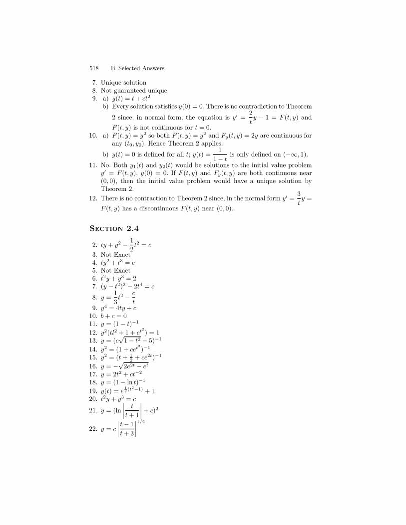
518 B Selected Answers
7. Unique solution8. Not guaranteed unique9. a) y(t) = t+ ct2
b) Every solution satisfies y(0) = 0. There is no contradiction to Theorem
2 since, in normal form, the equation is y′ =2
ty − 1 = F (t, y) and
F (t, y) is not continuous for t = 0.10. a) F (t, y) = y2 so both F (t, y) = y2 and Fy(t, y) = 2y are continuous for
any (t0, y0). Hence Theorem 2 applies.
b) y(t) = 0 is defined for all t; y(t) =1
1− t is only defined on (−∞, 1).
11. No. Both y1(t) and y2(t) would be solutions to the initial value problemy′ = F (t, y), y(0) = 0. If F (t, y) and Fy(t, y) are both continuous near(0, 0), then the initial value problem would have a unique solution byTheorem 2.
12. There is no contraction to Theorem 2 since, in the normal form y′ =3
ty =
F (t, y) has a discontinuous F (t, y) near (0, 0).
Section 2.4
2. ty + y2 − 1
2t2 = c
3. Not Exact4. ty2 + t3 = c5. Not Exact6. t2y + y3 = 27. (y − t2)2 − 2t4 = c
8. y =1
3t2 − c
t9. y4 = 4ty + c
10. b+ c = 011. y = (1− t)−1
12. y2(tl2 + 1 + et2) = 113. y = (c
√1− t2 − 5)−1
14. y2 = (1 + cet2)−1
15. y2 = (t+ 12 + ce2t)−1
16. y = −√
2e2t − et
17. y = 2t2 + ct−2
18. y = (1− ln t)−1
19. y(t) = e12 (t2−1) + 1
20. t2y + y3 = c
21. y = (ln
∣
∣
∣
∣
t
t+ 1
∣
∣
∣
∣
+ c)2
22. y = c
∣
∣
∣
∣
t− 1
t+ 3
∣
∣
∣
∣
1/4
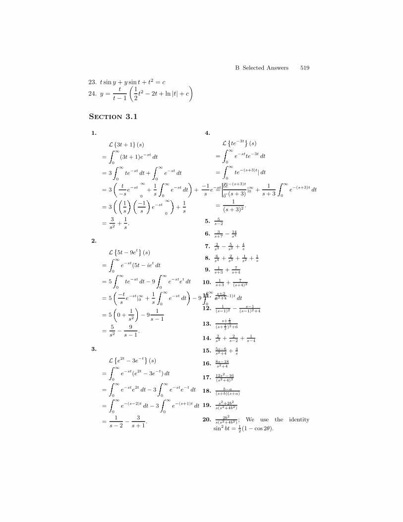
B Selected Answers 519
23. t sin y + y sin t+ t2 = c
24. y =t
t− 1
(
1
2t2 − 2t+ ln |t|+ c
)
Section 3.1
1.
L3t + 1 (s)
= ∞
0
(3t + 1)e−st dt
= 3 ∞
0
te−st dt + ∞
0
e−st dt
= 3 t
−se−st ∞0 +
1
s ∞
0
e−st dt+−1
se−st ∞0
= 3 1
s −1
s e−st ∞0 +1
s
=3
s2+
1
s.
2.
L 5t − 9et (s)
= ∞
0
e−st(5t − iet dt
= 5 ∞
0
te−st dt − 9 ∞
0
e−stet dt
= 5 −t
se−st|∞0 +
1
s ∞
0
e−st dt− 9 ∞
0
e−(s−1)t dt
= 5 0 +1
s2 − 91
s − 1
=5
s2− 9
s − 1.
3.
L e2t − 3e−t (s)
= ∞
0
e−st(e2t − 3e−t) dt
= ∞
0
e−ste2t dt − 3 ∞
0
e−ste−t dt
= ∞
0
e−(s−2)t dt − 3 ∞
0
e−(s+1)t dt
=1
s − 2− 3
s + 1.
4.
L te−3t (s)
= ∞
0
e−stte−3t dt
= ∞
0
te−(s+3)t| dt
=te−(s+3)t
−(s + 3)|∞0 +
1
s + 3 ∞
0
e−(s+3)t dt
=1
(s + 3)2.
5. 5s−2
6. 3s+7
− 14s4
7. 2s3 − 5
s2 + 4s
8. 6s4 + 2
s3 + 1s2 + 1
s
9. 1s+3
+ 7s+4
10. 1s+3
+ 7(s+4)2
11. s+2s2+4
12. 1(s−1)2
− s−1(s−1)2+4
13.s+ 1
3
(s+ 13)2+6
14. 2s3 + 2
s−2+ 1
s−4
15. 5s−6s2+4
+ 4s
16. 8s−18s2+4
17. 12s2−16(s2+4)3
18. b−a(s+b)(s+a)
19. s2+2b2
s(s2+4b2)
20. 2b2
s(s2+4b2); We use the identity
sin2 bt = 12(1 − cos 2θ).
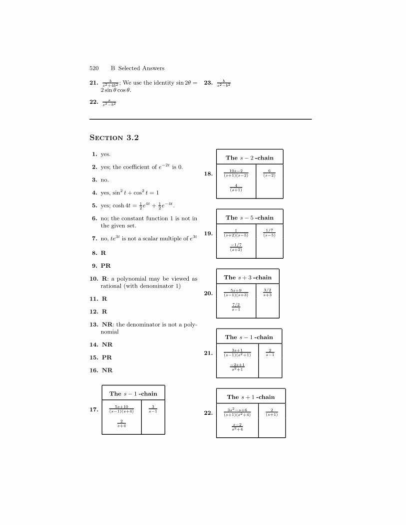
520 B Selected Answers
21. bs2+4b2
; We use the identity sin 2θ =2 sin θ cos θ.
22. ss2−b2
23. bs2−b2
Section 3.2
1. yes.
2. yes; the coefficient of e−2t is 0.
3. no.
4. yes, sin2 t + cos2 t = 1
5. yes; cosh 4t = 12e4t + 1
2e−4t.
6. no; the constant function 1 is not inthe given set.
7. no, te3t is not a scalar multiple of e3t
8. R
9. PR
10. R: a polynomial may be viewed asrational (with denominator 1)
11. R
12. R
13. NR: the denominator is not a poly-nomial
14. NR
15. PR
16. NR
17.
The s − 1 -chain
5s+10(s−1)(s+4)
3s−1
2s+4
18.
The s − 2 -chain
10s−2(s+1)(s−2)
6(s−2)
4(s+1)
19.
The s − 5 -chain
1(s+2)(s−5)
1/7(s−5)
−1/7(s+2)
20.
The s + 3 -chain
5s+9(s−1)(s+3)
3/2s+3
7/2s−1
21.
The s − 1 -chain
3s+1(s−1)(s2+1)
2s−1
−2s+1s2+1
22.
The s + 1 -chain
3s2−s+6(s+1)(s2+4)
2(s+1)
s−2s2+4
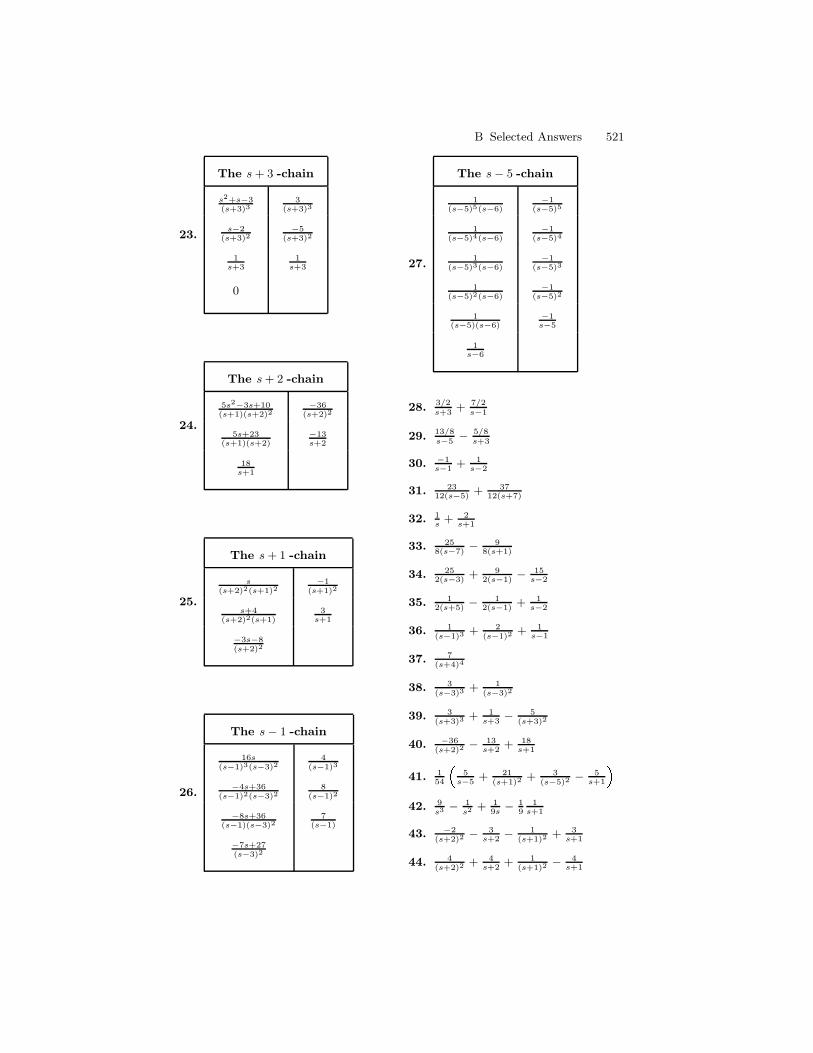
B Selected Answers 521
23.
The s + 3 -chain
s2+s−3(s+3)3
3(s+3)3
s−2(s+3)2
−5(s+3)2
1s+3
1s+3
0
24.
The s + 2 -chain
5s2−3s+10(s+1)(s+2)2
−36(s+2)2
5s+23(s+1)(s+2)
−13s+2
18s+1
25.
The s + 1 -chain
s(s+2)2(s+1)2
−1(s+1)2
s+4(s+2)2(s+1)
3s+1
−3s−8(s+2)2
26.
The s − 1 -chain
16s(s−1)3(s−3)2
4(s−1)3
−4s+36(s−1)2(s−3)2
8(s−1)2
−8s+36(s−1)(s−3)2
7(s−1)
−7s+27(s−3)2
27.
The s − 5 -chain
1(s−5)5(s−6)
−1(s−5)5
1(s−5)4(s−6)
−1(s−5)4
1(s−5)3(s−6)
−1(s−5)3
1(s−5)2(s−6)
−1(s−5)2
1(s−5)(s−6)
−1s−5
1s−6
28. 3/2s+3
+ 7/2s−1
29. 13/8s−5
− 5/8s+3
30. −1s−1
+ 1s−2
31. 2312(s−5)
+ 3712(s+7)
32. 1s
+ 2s+1
33. 258(s−7)
− 98(s+1)
34. 252(s−3)
+ 92(s−1)
− 15s−2
35. 12(s+5)
− 12(s−1)
+ 1s−2
36. 1(s−1)3
+ 2(s−1)2
+ 1s−1
37. 7(s+4)4
38. 3(s−3)3
+ 1(s−3)2
39. 3(s+3)3
+ 1s+3
− 5(s+3)2
40. −36(s+2)2
− 13s+2
+ 18s+1
41. 154
5
s−5+ 21
(s+1)2+ 3
(s−5)2− 5
s+142. 9
s3 − 1s2 + 1
9s− 1
91
s+1
43. −2(s+2)2
− 3s+2
− 1(s+1)2
+ 3s+1
44. 4(s+2)2
+ 4s+2
+ 1(s+1)2
− 4s+1
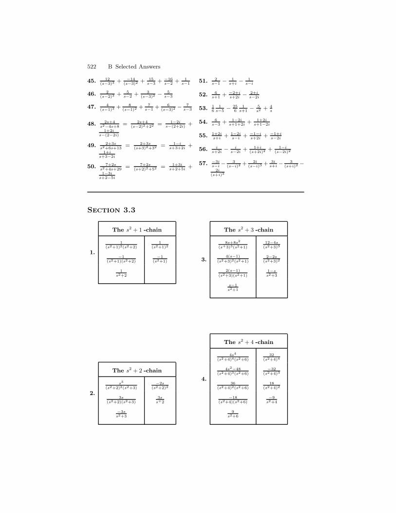
522 B Selected Answers
45. 12(s−3)3
+ −14(s−3)2
+ 15s−3
+ −16s−2
+ 1s−1
46. 2(s−2)3
+ 5s−2
+ 3(s−3)2
− 5s−3
47. 4(s−1)3
+ 8(s−1)2
+ 7s−1
+ 6(s−3)2
− 7s−3
48. 2s+4s2−4s+8
= 2s+4(s−2)2+22 = 1−2i
s−(2+2i)+
1+2is−(2−2i)
49. 2+3ss2+6s+13
= 2+3s(s+3)2+32 = 1−i
s+3+2i+
1+is+3−2i
50. 7+2ss2+4s+29
= 7+2s(s+2)2+52 = 1+3i
s+2+5i+
1−3is+2−5i
51. 2s−1
− 1s+i
− 1s−i
52. 6s+1
+ −2+is+2i
− 2+is−2i
53. 16
1s−5
− 256
1s+1
− 5s2 + 4
s
54. 6s−3
+ 1−2is+1+2i
+ 1+2is+1−2i
55. 1+2is+i
+ 1−2is−i
+ −1−is+2i
+ −1+is−2i
56. is+2i
− is−2i
+ 1+i(s+2i)2
+ 1−i(s−2i)2
57. −3is−i
− 3(s−i)2
+ 2i(s−i)3
+ 3is+i
− 3(s+i)2
−2i
(s+i)3
Section 3.3
1.
The s2 + 1 -chain
1(s2+1)2(s2+2)
1(s2+1)2
−1(s2+1)(s2+2)
−1(s2+1)
1s2+2
2.
The s2 + 2 -chain
s3
(s2+2)2(s2+3)−2s
(s2+2)2
3s(s2+2)(s2+3)
3ss+2
−3ss2+3
3.
The s2 + 3 -chain
8s+8s2
(s+3)3(s2+1)12−4s
(s2+3)3
4(s−1)
(s2+3)2(s2+1)2−2s
(s2+3)2
2(s−1)
(s2+3)(s2+1)1−ss2+3
s−1s2+1
4.
The s2 + 4 -chain
4s4
(s2+4)4(s2+6)32
(s2+4)4
4s2−48(s2+4)3(s2+6)
−32(s2+4)3
36(s2+4)2(s2+6)
18(s2+4)2
−18(s2+4)(s2+6)
−9s2+4
9s2+6
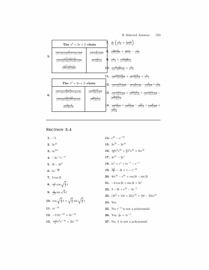
B Selected Answers 523
5.
The s2 + 2s + 2 -chain
1(s2+2s+2)2(s2+2s+3)2
1(s2+2s+2)2
−(s2+2s+4)
(s2+2s+2)(s2+2s+3)2−2
s2+2s+2
2s2+4s+7(s2+2s+3)2
6.
The s2 + 2s + 2 -chain
5s−5(s2+2s+2)2(s2+4s+5)
5s+5(s2+2s+2)2
−5s−15(s2+2s+2)(s2+4s+5)
3s−1s2+2s+2
−3s−5s2+4s+5
7. 110
3
s−3+ 1−3s
s2+18. 2s+2
(s2+1)2+ s−1
s2+1− 1
s+1
9. 2s−3
+ 6−2s(s−3)2+1
10. 9−3s((s−2)2+9)
+ 3s−1
11. −5s+15(s2−4s+8)2
+ −s+3s2−4s+8
+ 1s−1
12. −s(s2+6s+10)2
− ss2+6s+10
− 3(s+3)2
+ 1s+3
13. s+1(s2+4s+6)2
+ 2s+2s2+4s+6
+ s+1(s2+4s+5)2
−2s+2
s2+4s+5
14. −5(s2+5)3
+ 11(s2+5)2
− 17s2+5
+ 6(s2+6)2
+17
s2+6
Section 3.4
1. −5
2. 3e4t
3. 4e2it
4. −3e−te−it
5. 3t − 2t2
6. 2e−3t2
7. 3 cos 2t
8. −23
cos 023
t
9. 2√3
sin√
3 t
10. cos 023
t + 023
sin 023
t
11. te−3t
12. −11te−3t + 2e−3t
13. −112
t2e−3t + 2te−3t
14. e2t − e−4t
15. 3e3t − 2e2t
16. −16
t3e2t + 32t2e2t + 2te2t
17. 4e5t − 2et
18. tet + et + te−t − e−t
19. 9t2
2− 3t + 1 − e−3t
20. 4te2t − e2t + cos 2t − sin 2t
21. −2 cos 3t + sin 3t + 2et
22. 3 − 6t + e2t − 4e−t
23. (3t2 + 14t + 22)e3t + (8t − 22)e4t
24. Yes.
25. No; t−2 is not a polynomial.
26. Yes; tet = te−t.
27. No; 1t
is not a polynomial.
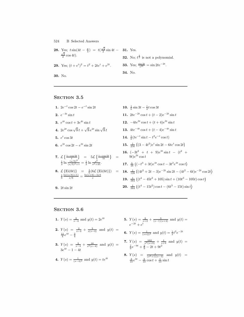
524 B Selected Answers
28. Yes; t sin(4t − π4) = t(
√2
2sin 4t −
√2
2cos 4t).
29. Yes; (t + et)2 = t2 + 2tet + e2t.
30. No.
31. Yes.
32. No; t12 is not a polynomial.
33. Yes; sin 2te2t = sin 2te−2t.
34. No.
Section 3.5
1. 2e−t cos 2t − e−t sin 2t
2. e−3t sin t
3. e4t cos t + 3e4t sin t
4. 2e2t cos√
8 t +√
8 e2t sin√
8 t
5. et cos 3t
6. e3t cos 2t − e3t sin 2t
7. L 1−cos 5tt
= 5L 1−cos 5t5t
=12
ln (s/5)2
(s/5)2+1= 1
2ln s2
s2+25.
8. LEi(6t) = 16(6LEi(6t)) =
16
ln((s/6)+1)s/6
= ln(s+6)−ln 6s
9. 2t sin 2t
10. 16
sin 3t − 12t cos 3t
11. 2te−2t cos t + (t − 2)e−2t sin t
12. −4te3t cos t + (t + 4)e3t sin t
13. 4te−4t cos t + (t − 4)e−4t sin t
14. 18(te−t sin t − t2e−t cos t)
15. 1256 (3 − 4t2)et sin 2t − 6tet cos 2t
16. (−3t2 + t + 9)e3t sin t − (t2 +9t)e3t cos t
17. 148 (−t3 + 3t)e4t cos t − 3t2e4t cos t
18. 1128 (4t2 + 2t − 3)e−2t sin 2t − (4t2 − 6t)e−2t cos 2t
19. 1384 (t4 − 45t2 + 105) sin t + (10t3 − 105t) cos t
20. 1384 (t4 − 15t2) cos t − (6t3 − 15t) sin t
Section 3.6
1. Y (s) = 2s−4
and y(t) = 2e4t
2. Y (s) = 2s−4
+ 3s(s−4)
and y(t) =114
e4t − 34
3. Y (s) = 2s−4
+ 16s2(s−4)
and y(t) =
3e4t − 1 − 4t
4. Y (s) = 1(s−4)2
and y(t) = te4t
5. Y (s) = 2s+2
+ 3(s−1)(s+2)
and y(t) =
e−2t + et
6. Y (s) = 1(s+2)3
and y(t) = 12t2e−2t
7. Y (s) = 162s3(s+9)
+ 1s+9
and y(t) =79e−9t + 2
9− 2t + 9t2
8. Y (s) = s(s2+1)(s−3)
and y(t) =310
e3t − 310
cos t + 110
sin t
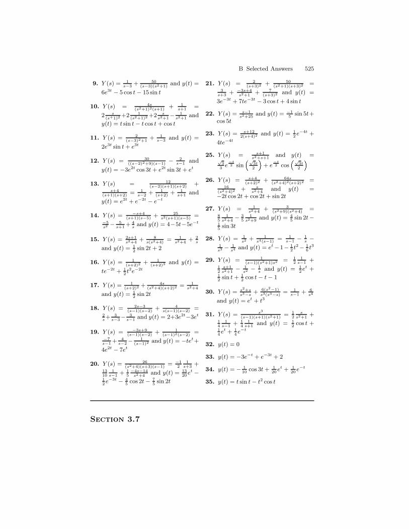
B Selected Answers 525
9. Y (s) = 1s−3
+ 50(s−3)(s2+1)
and y(t) =
6e3t − 5 cos t − 15 sin t
10. Y (s) = 4s(s2+1)2(s+1)
+ 1s+1
=
2 s(s+1)2
+2 1(s2+1)2
+2 ss2+1
− 1s2+1
and
y(t) = t sin t − t cos t + cos t
11. Y (s) = 2(s−3)2+1
+ 1s−3
and y(t) =
2e3t sin t + e3t
12. Y (s) = 30((s−2)2+9)(s−1)
− 2s−1
and
y(t) = −3e2t cos 3t + e2t sin 3t + et
13. Y (s) = 12(s−2)(s+1)(s+2)
+s+4
(s+1)(s+2)= 1
s−2+ 1
(s+2)+ 1
s+1and
y(t) = e2t + e−2t − e−t
14. Y (s) = −s+4(s+1)(s−5)
+ 25s2(s+1)(s−5)
=−5s2 − 5
s+1+ 4
sand y(t) = 4−5t−5e−t
15. Y (s) = 2s+1s2+4
+ 8s(s2+4)
= 1s2+4
+ 2s
and y(t) = 12
sin 2t + 2
16. Y (s) = 1(s+2)2
+ 1(s+2)3
and y(t) =
te−2t + 12t2e−2t
17. Y (s) = 1(s+2)2
+ 4s(s2+4)(s+2)2
= 1s2+4
and y(t) = 12
sin 2t
18. Y (s) = 2s−3(s−1)(s−2)
+ 4s(s−1)(s−2)
=2s+ 3
s−3− 3
s−1and y(t) = 2+3e2t−3et
19. Y (s) = −3s+9(s−1)(s−2)
+ 1(s−1)2(s−2)
=−7s−1
+ 4s−2
− 1(s−1)2
and y(t) = −tet+
4e2t − 7et
20. Y (s) = 26(s2+4)(s+3)(s−1)
= −12
1s+3
+1310
1s−1
+ 15
−4s−14s2+4
and y(t) = 1320
et −12e−3t − 4
5cos 2t − 7
5sin 2t
21. Y (s) = 2(s+3)2
+ 50(s2+1)(s+3)2
=3
s+3+ −3s+4
s2+1+ 7
(s+3)2and y(t) =
3e−3t + 7te−3t − 3 cos t + 4 sin t
22. Y (s) = s−1s2+25
and y(t) = −15
sin 5t+cos 5t
23. Y (s) = s+122(s+4)2
and y(t) = 12e−4t +
4te−4t
25. Y (s) = s+1s2+s+1
and y(t) =√
33
e−t2 sin
√3t2 + e
−t2 cos
√3t2
26. Y (s) = s+4(s+2)2
+ 64s(s2+4)2(s+2)2
=16
(s2+4)2+ s
s2+4and y(t) =
−2t cos 2t + cos 2t + sin 2t
27. Y (s) = 1s2+4
+ 3(s2+9)(s2+4)
=85
1s2+4
− 35
1s2+9
and y(t) = 45
sin 2t−15
sin 3t
28. Y (s) = 1s2 + 1
s4(s−1)= 1
s−1− 1
s−
1s3 − 1
s4 and y(t) = et −1− 12t2 − 1
6t3
29. Y (s) = 1(s−1)(s2+1)s2 = 1
21
s−1+
12
s+1s2+1
− 1s2 − 1
sand y(t) = 1
2et +
12
sin t + 12
cos t − t − 1
30. Y (s) = s2+ss3−s
+ 6(s2−1)
s3(s3−s)= 1
s−1+ 6
s4
and y(t) = et + t3
31. Y (s) = s3
(s−1)(s+1)(s2+1)= 1
2s
s2+1+
14
1s−1
+ 14
1s+1
and y(t) = 12
cos t +14et + 1
4e−t
32. y(t) = 0
33. y(t) = −3e−t + e−3t + 2
34. y(t) = − 110
cos 3t + 120
et + 120
e−t
35. y(t) = t sin t − t2 cos t
Section 3.7
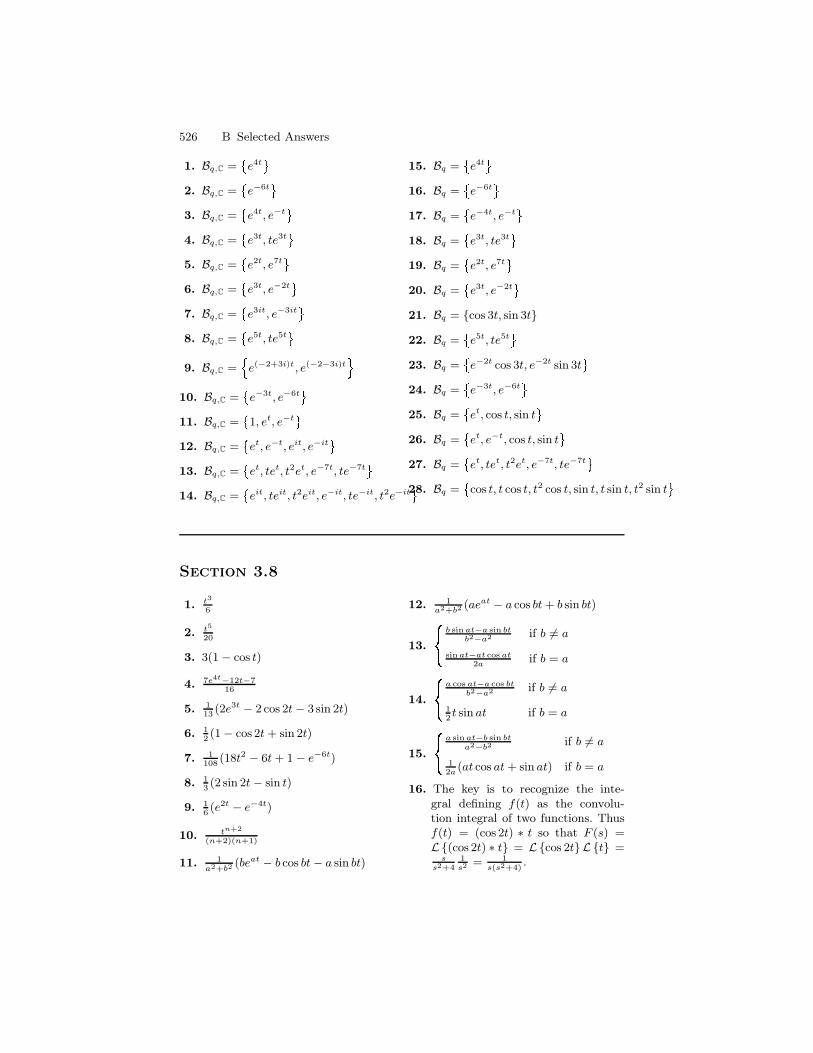
526 B Selected Answers
1. Bq,C = e4t 2. Bq,C = e−6t 3. Bq,C = e4t, e−t 4. Bq,C = e3t, te3t 5. Bq,C = e2t, e7t 6. Bq,C = e3t, e−2t 7. Bq,C = e3it, e−3it 8. Bq,C = e5t, te5t 9. Bq,C = 1e(−2+3i)t, e(−2−3i)t 2
10. Bq,C = e−3t, e−6t 11. Bq,C = 1, et, e−t12. Bq,C = et, e−t, eit, e−it13. Bq,C = et, tet, t2et, e−7t, te−7t14. Bq,C = eit, teit, t2eit, e−it, te−it, t2e−it
15. Bq = e4t 16. Bq = e−6t 17. Bq = e−4t, e−t18. Bq = e3t, te3t 19. Bq = e2t, e7t 20. Bq = e3t, e−2t 21. Bq = cos 3t, sin 3t
22. Bq = e5t, te5t 23. Bq = e−2t cos 3t, e−2t sin 3t24. Bq = e−3t, e−6t 25. Bq = et, cos t, sin t26. Bq = et, e−t, cos t, sin t27. Bq = et, tet, t2et, e−7t, te−7t 28. Bq = cos t, t cos t, t2 cos t, sin t, t sin t, t2 sin t
Section 3.8
1. t3
6
2. t5
20
3. 3(1 − cos t)
4. 7e4t−12t−716
5. 113
(2e3t − 2 cos 2t − 3 sin 2t)
6. 12(1 − cos 2t + sin 2t)
7. 1108
(18t2 − 6t + 1 − e−6t)
8. 13(2 sin 2t − sin t)
9. 16(e2t − e−4t)
10. tn+2
(n+2)(n+1)
11. 1a2+b2
(beat − b cos bt − a sin bt)
12. 1a2+b2
(aeat − a cos bt + b sin bt)
13. b sin at−a sin btb2−a2 if b 6= a
sin at−at cos at2a
if b = a
14. a cos at−a cos btb2−a2 if b 6= a
12t sin at if b = a
15. a sin at−b sin bta2−b2
if b 6= a
12a
(at cos at + sin at) if b = a
16. The key is to recognize the inte-gral defining f(t) as the convolu-tion integral of two functions. Thusf(t) = (cos 2t) ∗ t so that F (s) =L(cos 2t) ∗ t = Lcos 2tL t =
ss2+4
1s2 = 1
s(s2+4).
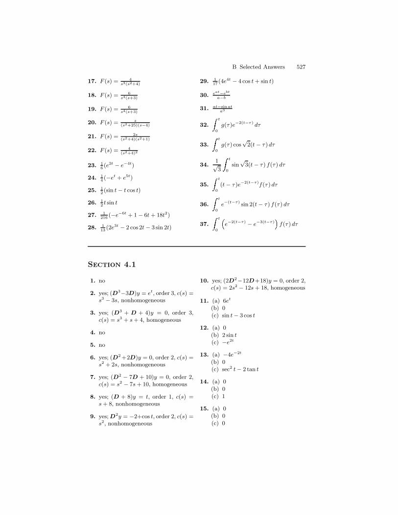
B Selected Answers 527
17. F (s) = 4s3(s2+4)
18. F (s) = 6s4(s+3)
19. F (s) = 6s4(s+3)
20. F (s) = s(s2+25)(s−4)
21. F (s) = 2s(s2+4)(s2+1)
22. F (s) = 4(s2+4)2
23. 16(e2t − e−4t)
24. 14(−et + e5t)
25. 12(sin t − t cos t)
26. 12t sin t
27. 1216
(−e−6t + 1 − 6t + 18t2)
28. 113
(2e3t − 2 cos 2t − 3 sin 2t)
29. 117
(4e4t − 4 cos t + sin t)
30. eat−ebt
a−b
31. at−sinata3
32. t
0
g(τ )e−2(t−τ) dτ
33. t
0
g(τ ) cos√
2(t − τ ) dτ
34.1√3
t
0
sin√
3(t − τ ) f(τ ) dτ
35. t
0
(t − τ )e−2(t−τ)f(τ ) dτ
36. t
0
e−(t−τ) sin 2(t − τ ) f(τ ) dτ
37. t
0
e−2(t−τ) − e−3(t−τ)f(τ ) dτ
Section 4.1
1. no
2. yes; (D3−3D)y = et, order 3, c(s) =s3 − 3s, nonhomogeneous
3. yes; (D3 + D + 4)y = 0, order 3,c(s) = s3 + s + 4, homogeneous
4. no
5. no
6. yes; (D2 +2D)y = 0, order 2, c(s) =s2 + 2s, nonhomogeneous
7. yes; (D2 − 7D + 10)y = 0, order 2,c(s) = s2 − 7s + 10, homogeneous
8. yes; (D + 8)y = t, order 1, c(s) =s + 8, nonhomogeneous
9. yes;D2y = −2+cos t, order 2, c(s) =s2, nonhomogeneous
10. yes; (2D2−12D+18)y = 0, order 2,c(s) = 2s2 − 12s + 18, homogeneous
11. (a) 6et
(b) 0
(c) sin t − 3 cos t
12. (a) 0
(b) 2 sin t(c) −e2t
13. (a) −4e−2t
(b) 0(c) sec2 t − 2 tan t
14. (a) 0
(b) 0
(c) 1
15. (a) 0(b) 0
(c) 0
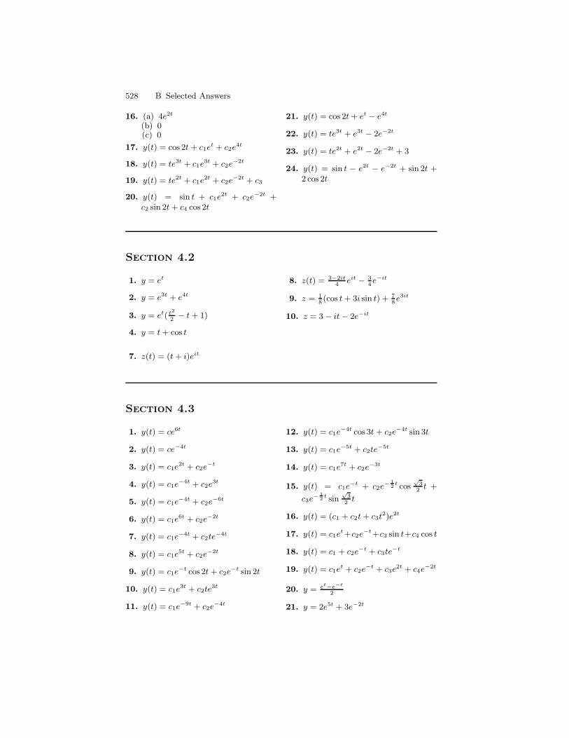
528 B Selected Answers
16. (a) 4e2t
(b) 0(c) 0
17. y(t) = cos 2t + c1et + c2e
4t
18. y(t) = te3t + c1e3t + c2e
−2t
19. y(t) = te2t + c1e2t + c2e
−2t + c3
20. y(t) = sin t + c1e2t + c2e
−2t +c2 sin 2t + c4 cos 2t
21. y(t) = cos 2t + et − e4t
22. y(t) = te3t + e3t − 2e−2t
23. y(t) = te2t + e2t − 2e−2t + 3
24. y(t) = sin t − e2t − e−2t + sin 2t +2 cos 2t
Section 4.2
1. y = et
2. y = e3t + e4t
3. y = et( t2
2− t + 1)
4. y = t + cos t
7. z(t) = (t + i)eit
8. z(t) = 3−2it4
eit − 34e−it
9. z = 18(cos t + 3i sin t) + 7
8e3it
10. z = 3 − it − 2e−it
Section 4.3
1. y(t) = ce6t
2. y(t) = ce−4t
3. y(t) = c1e2t + c2e
−t
4. y(t) = c1e−4t + c2e
3t
5. y(t) = c1e−4t + c2e
−6t
6. y(t) = c1e6t + c2e
−2t
7. y(t) = c1e−4t + c2te
−4t
8. y(t) = c1e5t + c2e
−2t
9. y(t) = c1e−t cos 2t + c2e
−t sin 2t
10. y(t) = c1e3t + c2te
3t
11. y(t) = c1e−9t + c2e
−4t
12. y(t) = c1e−4t cos 3t + c2e
−4t sin 3t
13. y(t) = c1e−5t + c2te
−5t
14. y(t) = c1e7t + c2e
−3t
15. y(t) = c1e−t + c2e
− 12
t cos√
32
t +
c3e− 1
2t sin
√3
2t
16. y(t) = (c1 + c2t + c3t2)e2t
17. y(t) = c1et+c2e
−t+c3 sin t+c4 cos t
18. y(t) = c1 + c2e−t + c3te
−t
19. y(t) = c1et + c2e
−t + c3e2t + c4e
−2t
20. y = et−e−t
2
21. y = 2e5t + 3e−2t
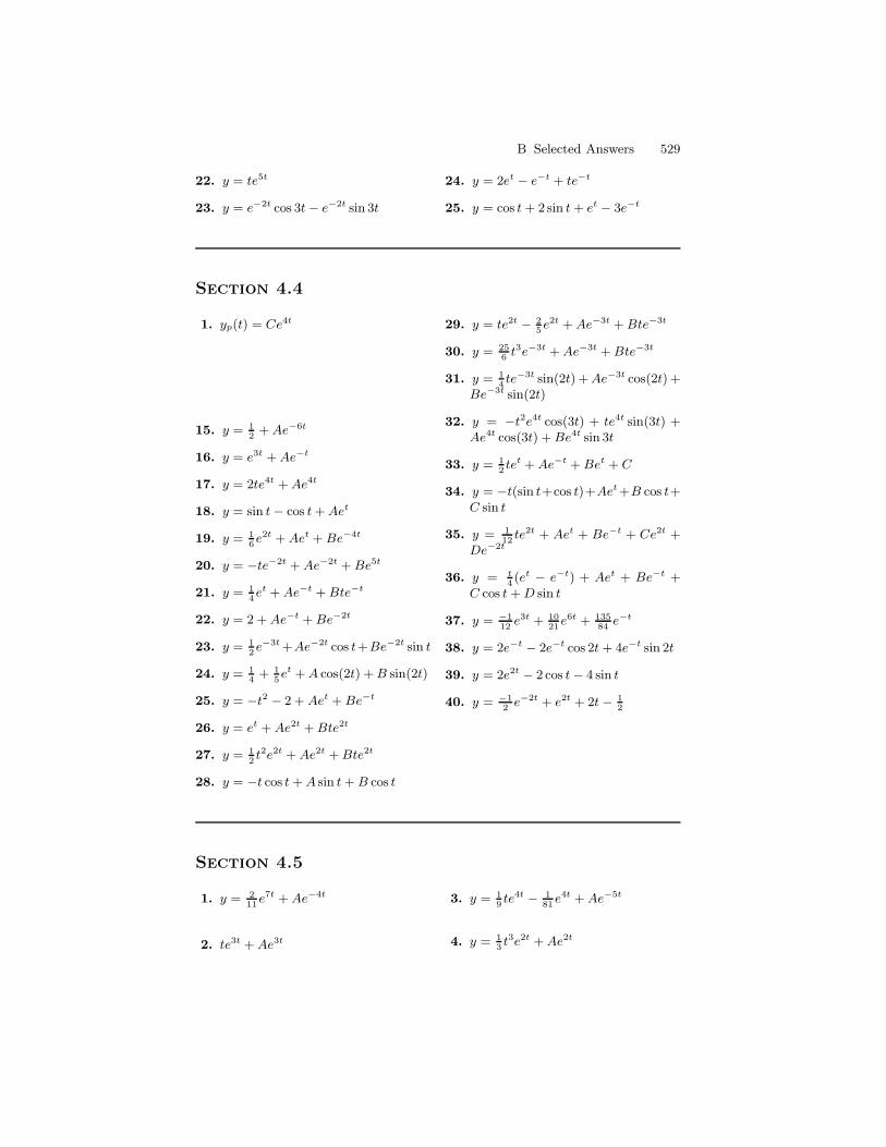
B Selected Answers 529
22. y = te5t
23. y = e−2t cos 3t − e−2t sin 3t
24. y = 2et − e−t + te−t
25. y = cos t + 2 sin t + et − 3e−t
Section 4.4
1. yp(t) = Ce4t
15. y = 12
+ Ae−6t
16. y = e3t + Ae−t
17. y = 2te4t + Ae4t
18. y = sin t − cos t + Aet
19. y = 16e2t + Aet + Be−4t
20. y = −te−2t + Ae−2t + Be5t
21. y = 14et + Ae−t + Bte−t
22. y = 2 + Ae−t + Be−2t
23. y = 12e−3t +Ae−2t cos t+Be−2t sin t
24. y = 14
+ 15et + A cos(2t) + B sin(2t)
25. y = −t2 − 2 + Aet + Be−t
26. y = et + Ae2t + Bte2t
27. y = 12t2e2t + Ae2t + Bte2t
28. y = −t cos t + A sin t + B cos t
29. y = te2t − 25e2t + Ae−3t + Bte−3t
30. y = 256
t3e−3t + Ae−3t + Bte−3t
31. y = 14te−3t sin(2t) + Ae−3t cos(2t) +
Be−3t sin(2t)
32. y = −t2e4t cos(3t) + te4t sin(3t) +Ae4t cos(3t) + Be4t sin 3t
33. y = 12tet + Ae−t + Bet + C
34. y = −t(sin t+cos t)+Aet +B cos t+C sin t
35. y = 112
te2t + Aet + Be−t + Ce2t +De−2t
36. y = t4(et − e−t) + Aet + Be−t +
C cos t + D sin t
37. y = −112
e3t + 1021
e6t + 13584
e−t
38. y = 2e−t − 2e−t cos 2t + 4e−t sin 2t
39. y = 2e2t − 2 cos t − 4 sin t
40. y = −12
e−2t + e2t + 2t − 12
Section 4.5
1. y = 211
e7t + Ae−4t
2. te3t + Ae3t
3. y = 19te4t − 1
81e4t + Ae−5t
4. y = 13t3e2t + Ae2t
530 B Selected Answers
5. y = 132
e−6t + Ae2t + Be−2t
6. y = −et + Ae−3t + Be5t
7. y = 15te−2t + Ae−2t + Be−3t
8. y = 2 + Ae−t + Be−2t
9. y = −te−4t + Ae2t + Be−4t
10. y = − 3130
cos t − 11130
sin t
11. y = −t2 + A + Be−3t + Ce3t
12. y = te2t − 25e2t + Ae−3t + Bte−3t
13. y = −te4t − 310
e4t + Ae−t + Be6t
14. y = −t2e4t cos(3t) + te4t sin(3t) +Ae4t cos(3t) + Be4t sin 3t
15. y = 16t3e2t + Ae2t + Bte2t
16. y = 12
sin t + Ae−t + Bte−t
17. y = 12tet sin t
18. 13t sin t + 1
9cos t + A + B cos(2t) +
C sin(2t)
19. y = 12tet + Ae−t + Bet + C
20. y = t4(et − e−t) + Aet + Be−t +
C cos t + D sin t
B Selected Answers 531
Section 6.1
1. no
2. yes, yes, homogeneous
3. yes, yes, nonhomogeneous
4. no
5. yes, yes, nonhomogeneous
6. yes, yes, nonhomogeneous
7. no
8. yes, yes, nonhomogeneous
9. yes, no, homogeneous
10. no
11. yes, no, homogeneous
12. yes, no, homogeneous
13. L(1) = 1′′ + 1 = 1L(t) = t′′ + t = tL(e−t) = (e−t)′′ + e−t = 2e−t
L(cos 2t) = (cos 2t)′′ + cos 2t =−4 cos 2t + cos 2t = −3 cos 2t.
14. L(1) = 1L(t) = tL(e−t) = (t + 1)e−t
L(cos 2t) = (−4t + 1) cos 2t
15. L(1) = −3L(t) = 1 − 3tL(e−t) = −2e−t
L(cos 2t) = −11 cos 2t − 2 sin 2t
16. L(1) = 5L(t) = 5t + 6L(e−t) = 0L(cos 2t) = cos 2t − 12 sin 2t
17. L(1) = −4L(t) = −4tL(e−t) = −3e−t
L(cos 2t) = −8 cos 2t
18. L(1) = −1L(t) = 0
L(e−t) = (t2 − t − 1)e−t
L(cos 2t) = (−4t2 − 1) cos 2t −2t sin 2t
19. L(ert) = a(ert)′′ + b(ert)′ + cert =ar2ert+brert+cert = (ar2+br+c)ert
20. C = −34
21. C1 = −34
and C2 = 12
22. no
23. yes, C = 1.
24. Parts (1) and (2) are done by com-puting y′′ + y where y(t) = t2 − 2,y(t) = cos t, or y(t) = sin t. Thenby Theorem 3, every function of theform y(t) = t2 − 2 + c1 cos t + c2 sin tis a solution to y′′ + y = t2, wherec1 and c2 are constants. If we want asolution to L(y) = t2 with y(0) = aand y′(0) = b, then we need to solvefor c1 and c2:
a = y(0) = −2 + c1
b = y′(0) = c2
These equations give c1 = a + 2,c2 = b. Particular choices of a and bgive the answers for Part (3).
(3)a. y = 12et + 2e2t − 3
2e3t
(3)b. y = 12et − 2e2t + 3
2e3t
(3)c. y = 12et − 7e2t + 11
2e3t
(3)d. y = 12et + (−1 + 3a − b)e2t +1
2− 2a + be3t
25.(3)a. y = 12et + 2e2t − 3
2e3t
(3)b. 12et − 2e2t + 3
2e3t
(3)c. 12et + 11
2e2t − 7e3t
(3)d. 12et + (3a− b− 1)e2t + (b− 2a +
12)e3t
26.(3)a. y = 16t5 + 10
3t2 − 5
2t3
(3)b. y = 16t5 − 2
3t2 + 1
2t3
(3)c. y = 16t5 − 17
3t2 + 9
2t3
532 B Selected Answers
(3)d. y = 16t5 + 1
3+ 3a − b t2 +− 1
2− 2a + b t3
27. Write the equation in the standardform:
y′′ +3
ty′ − 1
t2y = t2.
Then a1(t) =3
t, a2(t) = − 1
t2, and
f(t) = t2. These three functionsare all continuous on the intervals(0, ∞) and (−∞, 0). Thus, Theorem6 shows that if t0 ∈ (0, ∞) then theunique solution is also defined on theinterval (0, ∞), and if t0 ∈ (−∞, 0),then the unique solution is definedon (−∞, 0).
28. Maximal intervals are (−∞,−1),(−1, 1), (1, ∞)
29. (kπ, (k + 1)π) where k ∈ Z
30. (−∞, ∞)
31. (3, ∞)
32. (−∞, −2), (−2, 0), (0 2), (2, ∞)
33. The initial condition occurs at t = 0which is precisely where a2(t) = t2
has a zero. Theorem 6 does not ap-ply.
34. In this case y(t0) = 0 and y′(t0) = 0.The function y(t) = 0, t ∈ I is a so-lution to the initial value problem.By the uniqueness part of Theorem6 y = 0 is the only solution.
35. The assumptions say that y1(t0) =y2(t0) and y′
1(t0) = y′2(t0). Both y1
and y2 therefore satisfies the sameinitial conditions. By the uniquenesspart of Theorem 6 y1 = y2.
Section 6.2
1. dependent; 2t and 5t are multiples ofeach other.
2. independent
3. independent
4. dependent; e2t + 1 = e1e2t ande2t−3 = e−3e2t, they are multiplesof each other.
5. independent
6. dependent; ln t2 = 2 ln t and ln t5 =5 ln t, they are multiples of eachother.
7. dependent; sin 2t = 2 sin t cos t, theyare multiples of each other.
8. dependent; cosh t = 12(et + e−t) and
3et(1 + e−2t) = 3(et + e−t), they aremultiples of each other.
9. 1. Suppose at3 + b t3 = 0 on(−∞,∞). Then for t = 1 andt = −1 we get
a + b = 0
−a + b = 0.
These equations imply a = b =0. So y1 and y2 are linearly in-dependent.
2. Observe that y′1(t) = 3t2 and
y′2(t) = −3t2 if t < 0
3t2 if t ≥ 0.If
t < 0 then w(y1, y2)(t) =t3 −t3
3t2 −3t2 = 0. If t ≥ 0 then
w(y1, y2)(t) = t3 t3
3t2 3t2 = 0.
It follows that the Wronskian iszero for all t ∈ (−∞,∞).
3. The condition that the coeffi-cient function a2(t) be nonzero
B Selected Answers 533
in Theorem 4 and Proposition6 is essential. Here the coeffi-cient function, t2, of y′′ is zero att = 0, so Proposition 6 does notapply on (−∞,∞). The largestopen intervals on which t2 isnonzero are (−∞, 0) and (0,∞).On each of these intervals y1 andy2 are linearly dependent.
4. Consider the cases t < 0 andt ≥ 0. The verification is thenstraightforward.
5. Again the condition thatthe coefficient function a2(t)be nonzero is essential. TheUniqueness and Existence theo-rem does not apply.
Section 6.3
1. The indicial polynomial is q(s) =s2 + s − 2 = (s + 2)(s − 1). Thereare two distinct roots 1 and −2. Thefundamental set is t, t−2. The gen-eral solution is y(t) = c1t + c2t
−2.
2. The indicial polynomial is q(s) =2s2 − 7s + 3 = (2s − 1)(s − 3).There are two distinct roots 1
2and
3. The fundamental set is 1t12 , t32.
The general solution is y(t) = c1t12 +
c2t3.
3. The indicial polynomial is q(s) =9s2 − 6s + 1 = (3s − 1)2. There isone root, 1/3, with multiplicity 2.
The fundamental set is 1t13 , t
13 ln t2.
The general solution is y(t) = c1t13 +
c2t13 ln t.
4. The indicial polynomial is q(s) =s2 −2 = (s−
√2)(s+
√2). There are
two distinct roots√
2 and −√
2. Thefundamental set is 1t
√2, t−
√22. The
general solution is y(t) = c1t√
2 +
c2t−√
2.
5. The indicial polynomial is q(s) =4s2 −s+1 = (2s−1)2. The root is 1
2
with multiplicity 2. The fundamen-
tal set is 1t12 , t
12 ln t2. The general
solution is y(t) = c1t12 + c2t
12 ln t.
6. The indicial polynomial is q(s) =s2−4s−21 = (s−7)(s+3). The rootsare 7 and −3. The fundamental setis t7, t−3. The general solution isy(t) = c1t
7 + c2t−3.
8. The indicial polynomial is q(s) =s2 − s + 1 = s2 − s + 1/4 +3/4 = (s − 1/2)2 + (
√3/2)2.
There are two complex roots, 1+i√
32
and 1−i√
32
. The fundamental set
is 1t12 sin
√3
2t, t
12 cos
√3
2t2. The gen-
eral solution is y(t) = c1t12 sin
√3
2t +
c2t12 cos
√3
2t.
9. The indicial polynomial is q(s) =s2−4 = (s−2)(s+2). There are twodistinct roots, 2 and −2. The funda-mental set is t2, t−2. The generalsolution is y(t) = c1t
2 + c2t−2.
10. The indicial polynomial is q(s) =s2 +4. There are two complex roots,2i and −2i. The fundamental setis cos(2 ln t), sin(2 ln t). The gen-eral solution is y(t) = c1 cos(2 ln t)+c2 sin(2 ln t).
11. The indicial polynomial is q(s) =s2 − 4s + 13 = (s − 2)2 + 9.There are two complex roots, 2 +3i and 2 − 3i. The fundamen-tal set is t2 cos(3 ln t), t2 sin(3 ln t).
534 B Selected Answers
The general solution is y(t) =c1t
2 cos(3 ln t) + c2t2 sin(3 ln t).
12. y =1
3(t − t−2)
13. y = 2t1/2 − t1/2 ln t
14. y = −3 cos(2 ln t) + 2 sin(2 ln t)
15. No solution is possible.
Section 6.4
1. ln
s−as−b
2. ln
s2+b2
s2+a2 3. s ln
s2+a2
s2+b2 + 2b tan−1 bs −
2a tan−1 as
4. tan−1 as
5. y = at + bet
6. y = a(t + 1) + be−t
7. Y ′(s)+ 1s+1
Y (s) = 0 and Y (s) = Cs+1
and y(t) = Ce−t
8. Y ′(s) = −y0(s+2)2
, Y (s) = y0s+2
, and
y(t) = e−2t.
9. Y ′(s) + 4ss2+1
Y (s) = 3y0s2+1
. Solving
gives Y (s) = y0(s3+3s)+C
(s2+1)2and y(t) =
A(t cos t − sin t) + B(t sin t + cos t).
10. Y ′(s) + 2s2+s−2s(s−1)
= 2(y0s+y1)s(s−1)
Y (s) =
2s2−2s+12s2(s−1)
y0+ 2s−11s2(s−1)
y1 y(t) = (−t+
1 + et) + (t − 1 + et)y1 The generalsolution can be written A(t−1)+Bet
11. Y ′(s) = −y0(s+1)2
, Y (s) = y0s+1
, and
y(t) = y0e−t.
12. Y ′(s) + 6ss2+1
Y (s) = 0,
Y (s) = C(s2+1)3
, and y(t) =
C (3 − t2) sin t − 3t cos t13. Y ′(s)− s−2
s+1Y (s) = −sy0−y1
(s+1)2, Y (s) =
y0s2+3s+3(s+1)3
+ y1s+2
(s+1)3, and y(t) =
y0(e−t + te−t + t2
2e−t) + y1(te
−t +
t2
2e−t). The general solution can be
written y(t) = Ae−t + B(te−t +t2
2e−t).
14. Y ′(s) = y0(1s− 1
s−1) Then Y (s) =
y0 ln
ss−1+ C. Take C = 0. Hence
y(t) = y01−et
t.
15. Y ′(s) = −y0s2−1
and Y (s) =
y02
ln
s+1s−1 + C. Take C = 0 Then
y(t) = y02
et−e−t
t.
16. Y ′(s) = −y0(s2−5s+6)
and Y (s) =
y0 ln
s−2s−3 + C. Take C = 0. Then
y(t) = y0
e3t−e2t
t .
17. Y ′(s) = −y0s2+9
so Y (s) =−y03
(tan−1(s/3) + C). Sincelims→∞ Y (s) = 0 we have C = −π
2.
Hence Y (s) = y03
tan−1( 3s) and
y(t) = y03
sin 3tt
.
18. Y ′(s) = −y0s2+s
and hence y(s) =
y0 ln s+1s + C. But C = 0 and
y(t) = y01−e−t
t.
19. We use the formula
dn
dtn(f(t)g(t)) =
n k=0 n
m dk
dtkf(t)· dn−k
dtn−kg(t).
Observe that
dk
dtke−t = (−1)ke−t
and
dn−k
dtn−ktn = n(n − 1) · · · (k + 1)tk.
B Selected Answers 535
It now follows that
1
n!et dn
dtn(e−ttn)
=1
n!et
n k=0 n
k dk
dtke−t dn−k
dtn−ktn
= etn
k=0 n
k(−1)ke−t n(n − 1) · · · (k + 1)
n!tk
=
n k=0
(−1)k n
ktk
k!
= `n(t).
20. This follows in a similar manner tothe proof of Equation (2) given inTheorem 11.
21. F
22.
L`n(at) (s)
=n
k=0 n
k(−1)kakL tk
k! =
n k=0 n
k(−1)kak 1
sk+1
=1
sn+1
n k=0 n
k(−a)ksn−k
=(s − a)n
sn+1.
The last line follows from the bi-nomial theorem. Note: the dilationprinciple gives the same formula fora > 0.
23. Hint: Take the Laplace transform ofeach side. Use the previous exerciseand the binomial theorem.
24. We have that `n∗1(t) = t
0`n(x) dx.
By the convolution theorem
L`n ∗ 1 (s) =1
s
(s − 1)n
sn+1
= 1 − s − 1
s (s − 1)n
sn+1
=(s − 1)n
sn+1− (s − 1)n+1
sn+2
= L`n (s) − L`n+1 (s).
The result follows by inversion.
25. We compute the Laplace transformof both sides. We’ll do a piece at atime.
L(2n + 1)`n (s)
= (2n + 1)(s − 1)n
sn+1
=(s − 1)n−1
sn+2(2n + 1)(s(s − 1)).
L−t`n (s)
= (s − 1)n
sn+1 ′
=(s − 1)n−1
sn+2(n + 1 − s).
−nL`n−1 (s)
= −n(s − 1)n−1
sn
=(s − 1)n−1
sn+2(−ns2).
We have written each so that thecommon factor is (s−1)n−1
sn+2 . The co-efficients are
n + 1 − s + (2n + 1)(s(s − 1)) − ns2
= (n + 1)(s2 − 2s + 1)
= (n + 1)(s − 1)2
The right hand side is now
1
n + 1 (n + 1)(s − 1)2(s − 1)n−1
sn+2 =
(s − 1)n+1
sn+2
= L`n+1 (s).
Taking the inverse Laplace trans-form completes the verification.
536 B Selected Answers
26. We have that `n ∗ `m(t) = t
0`n(x)`m(t − x) dx. By the convo-
lution theorem
L`n ∗ `m (s)
=(s − 1)m
sm+1
(s − 1)n
sn+1
=(s − 1)m+n
sm+n+1 1 − s − 1
s =
(s − 1)m+n
sm+n+1− (s − 1)m+n+1
sm+n+2
= L`m+n(s) − L`m+n+1 (s).
The result follows by inversion.
27. First of all∞0
e−t`n(t) dt =L`n (1) = 0. Thus ∞
t
e−x`n(x) dt
= − t
0
e−x`n(x) dx
= −e−t ∞
0
et−x`n(x) dx
= −e−t(et ∗ `n(t)).
By the convolution theorem
L et ∗ `n(s)
=1
s − 1
(s − 1)n
sn+1
=(s − 1)n−1
sn+1
=(s − 1)n−1
sn 1 − s − 1
s =
(s − 1)n−1
sn− (s − 1)n
sn+1
= L−1 `n−1(t) − L−1 `n(t) .
It follows by inversion that et ∗ `n =`n−1 − `n and substituting this for-mula into the previous calculationgives the needed result.
28. F
Section 6.5
1. Let y2(t) = t2u(t). Then t4u′′ +t3u′ = 0, which gives u′ = t−1
and u(t) = ln t. Substituting givesy2(t) = t2 ln t. The general solutioncan be written y(t) = c1t
2 + c2t2 ln t.
2. y2(t) = −13t2
. The general solution canbe written y(t) = c1t + c2
1t2
.
3. Let y2(t) = (1−t2)u(t). Substitutiongives (1 − t2)2u′′ − 4t(1 − t2)u′ = 0
and hence u′′
u′ = −2 −2t1−t2
. From this
we get u′ = 1(1−t)2
. Integrating u′ by
partial fractions give u = −12
t1−t2
+
14
ln
1+t1−t and hence
y2(t) =−1
2t+
1
4(1− t2) ln 1 + t
1 − t .
4. y2(t) = −1 + t2
ln
1+t1−t . The gen-
eral solution can be written y(t) =
c1t + c2
−1 + t
2ln
1+t1−t .
5. Let y2(t) = t12 u(t). Then 4t
52 u′′ +
4t32 u′ = 0 leads to u′ = 1/t and
hence u(t) = ln t. Thus y2(t) =√t ln t. The general solution can be
written y(t) = c1
√t + c + 2
√t ln t.
6. y2(t) = 1. The general solution canbe written y(t) = c1t + c2.
7. y2(t) = tet. The general solution canbe written y(t) = c1t + c2te
t.
8. Let y2(t) = t2 cos t u(t). Thent4 cos t u′′ − 2t4 sin t u′ = 0 which
B Selected Answers 537
gives u′(t) = sec2 t and hence u(t) =tan t. Thus y2(t) = t2sin t. The gen-eral solution can be written y(t) =c1t
2cos t + c2t2sin t.
9. y2(t) = −12
cos t2. The general solu-tion can be written y(t) = c1 sin t2 +c2 cos t2.
10. y2(t) = te2t. The general solutioncan be written y(t) = c1e
2t + c2te2t.
11. y2(t) = −1 − t tan t. The gen-eral solution can be written y(t) =c1 tan t + c2(1 + t tan t).
12. y2(t) = t − 1. The general solutioncan be written y(t) = c1e
−t + c2(t−1).
13. y2(t) = − sec t. The general solu-tion can be written y(t) = c1 tan t +c2 sec t.
14. Let y2(t) = tu(t). Then (t3 + t)u′′ +
2u′ = 0 which gives u′ = t2+1t2
andu = t − 1
t. Thus y2(t) = t2 − 1.
The general solution can be writteny(t) = c1t + c2(t
2 − 1).
15. y2(t) = t sin t. The general solutioncan be written y(t) = c1t cos t +c2t sin t.
Section 6.6
1. sin t and cos t form a fundamental setfor the homogeneous solutions. Letyp(t) = u1 cos t + u2 sin t. Then thematrix equation cos t sin t− sin t cos t u′
1
u′2 = 0
sin t im-
plies u′1(t) = − sin2 t = 1
2(cos 2t − 1)
and u′2(t) = cos t sin t = 1
2(sin 2t).
Integration give u1(t) = 14(sin(2t) −
2t) = 12(sin t cos t − t) and u2(t) =
−14
cos 2t = −14
(2 cos 2t−1). This im-plies yp(t) = 1
4sin t − 1
2t cos t. Since
14
sin t is a homogeneous solution wecan write the general solution in theform y(t) = −1
2t cos t + c1 cos t +
c2 sin t. We observe that a particu-lar solution is the imaginary part ofa solution to y′′+y = eit. We use theincomplete partial fraction methodand get Y (s) = 1
(s−i)2(s+i). This
can be written Y (s) = 12i
1(s−i)2
+p(s)
(s−i)(s+i). From this we get yp(t) =
Im
12iL−1 1
(s−i)2 = Im −i
2teit =
−12
t cos t. The general solution isy(t) = −1
2t cos t + c1 cos t + c2 sin t.
See Example 3 in Section 4.5 for arelated problem.
2. A fundamental set for y′′ − 4y = 0is e2t, e−2t . Let yp(t) = u1(t)e
2t +u2(t)e
−2t. Then the matrix equatione2t e−2t
2e2t −2e−2t u′1
u′2 = 0
e2t im-
plies u′1(t) = 1
4and u′
2(t) = −e4t
4and
hence u1(t) = t4
and u2(t) = −e4t
16.
Now yp(t) = t4e2t − e2t
16. Since e2t
16
is a homogeneous solution we canwrite the general solution as y(t) =t4e2t + c1e
2t + c2e−2t. On the other
hand, the incomplete partial fractionmethod gives Y (s) = 1
(s−2)2(s+2=
14
(s−2)2+ p(s)
(s−2)(s+2). From this we see
that a particular solution is yp(t) =14te2t. The general solution is y(t) =
14te2t + c1e
2t + c2e−2t.
3. The functions et cos 2t and et sin 2tform a fundamental set. Let yp(t) =c1e
t cos 2t+c2et sin 2t. Then the ma-
trix equation
538 B Selected Answers
W (et cos 2t, et sin 2t) u′1
u′2 = 0
etimplies that u′
1(t) = −12
sin 2t andu′
2(t) = 12
cos 2t. Hence, u1(t) =14cos2t and u2(t) = 1
4sin 2t. From
this we get yp(t) = 14et cos2 2t +
14et sin2 2t = 1
4et. On the other
hand, the method of undeterminedcoefficients implies that a particularsolution is of the form yp(t) = Cet.Substitution gives 4Cet = et andhence C = 1
4. It follows that yp(t) =
14et. Furthermore, the general solu-
tion is y(t) = 14et + c1e
t cos 2t +c2e
t sin 2t.
4. A fundamental set is 1, e−3t . Thematrix equation1 e−3t
0 −3e−3t u′1
u′2 = 0
e−3t im-
plies u′1(t) = 1
3e−3t and u′
2(t) = −13
.
Thus u1(t) = −e−3t
9, u2(t) = −t
3,
and yp(t) = −e−3t
9− t
3e−3t. Ob-
serve though that −e−3t
9is a ho-
mogeneous solution and so the gen-eral solution can be written y(t) =− t
3e−3t + c1 + c2e
−3t. The incom-plete partial fraction method gives
Y (s) = 1(s+3)2s
=−13
(s+3)2+ p(s)
(s+3)s
which implies that −13
te−3t is a par-ticular solution. The general solutionis as above.
5. A fundamental set is et, e2t . Thematrix equationet e2t
et 2e2t u′1
u′2 = 0
e3t implies
u′1(t) = −e2t and u′
2(t) = et. Henceu1(t) = −1
2e2t, u2(t) = et, and
yp(t) = −12
e2tet + ete2t = 12e3t. The
general solution is y(t) = 12e3t +
c1et + c2e
2t. The method of undeter-mined coefficients implies that a par-ticular solution is of the form yp =Ce3t. Substitution gives 2Ce3t =3e3t and hence C = 1
2. The general
solution is as above.
6. sin t and cos t form a fundamental setfor the homogeneous solutions. Letyp(t) = u1 cos t + u2 sin t. Then thematrix equation cos t sin t− sin t cos t u′
1
u′2 = 0
tan t im-
plies that u′1(t) = cos t − sec t
and u′2(t) = sin t. From this we
get u1(t) = sin t − ln |sec t + tan t|and u2(t) = − cos t. Thereforeyp(t) = − cos t ln |sec t + tan t|. Thegeneral solution is thus y(t) =− cos t ln |sec t + tan t| + c1 cos t +c2 sin t.
7. A fundamental set is et, tet . Thematrix equationet tet
et et + tet u′1
u′2 = 0
et
t implies
u′1(t) = −1 and u′
2(t) = 1t. Hence,
u1(t) = −t, u2(t) = ln t, and yp(t) =−tet + t ln tet. Since −tet is a homo-geneous solution we can write thegeneral solution as y(t) = t ln tet +c1e
t + c2tet.
8. A fundamental set is cos t, sin t.The matrix equation cos t sin t− sin t cos t u′
1
u′2 = 0
sec t im-
plies u′1(t) = − tan t and u′
2(t) = 1.Hence u1(t) = ln(cos t), u2(t) = t,and yp(t) = cos t ln(cos t) + t sin t.The general solution is y(t) =cos t ln(cos t) + t sin t + c1 cos t +c2 sin t.
9. The associated homogeneous equa-tion is Cauchy-Euler with indicialequation s2 −3s+2 = (s−2)(s−1).It follows that t, t2 forms a funda-mental set. We put the given equa-tion is standard form to get y′′ −2ty′ + 2
t2y = t2. Thus f(t) = t2. The
matrix equationt t2
1 2t u′1
u′2 = 0
t2 implies
u′1(t) = −t2 and u′
2(t) = t. Hence
u1(t) = −t3
3, u2(t) = t2
2, and yp(t) =
B Selected Answers 539
−t3
3t + t2
2t2 = t4
6. It follows that the
general solution is y(t) = t4
6+ c1t +
c2t2.
10. In standard form we get y′′ −1ty′ = 3t − 1
t. The matrix equation1 t2
0 2t u′1
u′2 = 0
3t − 1t implies
u′1(t) = −3
2t2+ 1
2and u′
2(t) = 32− 1
2t2.
Hence u1(t) = −12
t3 + 12t, u2(t) =
32t+ 1
2t, and yp(t) = t3 + t. The gen-
eral solution is y(t) = t3+t+c1+c2t2.
11. The homogeneous equation isCauchy-Euler with indicial equations2 −2s+1 = (s−1)2. It follows thatt, t ln t is a fundamental set. Afterwriting in standard form we see theforcing function f(t) is 1
t. The ma-
trix equationt t ln t1 ln t + 1 u′
1
u′2 = 0
1t implies
u′1(t) = − ln t
tand u′
2(t) = 1t. Hence
u1(t) = − ln2 t2
, u2(t) = ln t, andyp(t) = −t
2ln2 t + t ln2 t = t
2ln2 t.
The general solution is y(t) =t2
ln2 t + c1t + c2t ln t.
12. A fundamental set is e2t, te2t .The matrix equatione2t te2t
2e2t e2t(1 + 2t) u′1
u′2 = 0
e2t
t2+1
implies u′1(t) = −t
t2+1and u′
2(t) =1
t2+1. Hence u1(t) = −1
2ln(t2 + 1),
u2(t) = tan−1 t, and yp(t) =−12
e2t ln(t2 + 1) + t tan−1 e2t.The general solution is y(t) =−12
e2t ln(t2+1)+t tan−1 e2t+c1e2t+
c2te2t.
13. The matrix equationtan t sec tsec2 t sec t tan t u′
1
u′2 = 0
t im-
plies u′1(t) = t and u′
2(t) = −t sin t.
Hence u1(t) = t2
2, u2(t) = t cos t −
sin t, and yp(t) = t2
2tan t + (t cos t−
sin t) sec t = t2
2tan t+ t− tan t. Since
tan t is a homogeneous solution wecan write the general solution asy(t) = t2
2tan t+ t+ c1 tan t+ c2 sec t.
14. When put in standard form one seesthat f(t) = te−t. The matrix equa-tiont − 1 e−t
1 −e−t u′1
u′2 = 0
te−t im-
plies u′1(t) = e−t and u′
2(t) = 1 − t.
Hence u1(t) = −e−t, u2(t) = t − t2
2,
and yp(t) = −(t − 1)e−t + (t −t2
2)e−t = −t2
2e−t + e−t. Since e−t
is a homogeneous solution we canwrite the general solution as y(t) =−t2
2e−t + c1(t − 1) + c2e
−t.
15. After put in standard form the forc-ing function f is 4t4. The matrixequation cos t2 sin t2
−2t sin t2 2t cos 2t u′1
u′2 =
04t4 implies u′
1(t) = −2t3 sin t2
and u′2(t) = 2t3 cos t2. Integration by
parts gives u1(t) = t2 cos t2 − sin t2
and u2(t) = t2 sin t2 + cos t2. Henceyp(t) = t2 cos t2 − cos t2 sin t2 +t2 sin t2 + cos t2 sin t2 = t2. The gen-eral solution is y(t) = t2 + c1 cos t2 +c2 sin t2.
16. A fundamental set is et, e−t. Thematrix equationet e−t
et −e−t u′1
u′2 = 0
11+e−t im-
plies u′1(t) = 1
21
1+et and u′2(t) =
−12
et
1+et . Hence u1(t) = 12(t − ln(1 +
et), u2(t) = −12
(et − ln(1 + et)), andyp(t) = 1
2(tet − 1 − (et − e−t) ln(1 +
et)). (Note: in the integrations ofu′
1 and u′2 use the substitution u =
et.) The general solution can nowbe written y(t) = 1
2(tet − 1 − (et −
e−t) ln(1 + et)) + c1et + c2e
−t.
540 B Selected Answers
Section 7
1. The ratio test gives (n+1)2
n2 → 1.R = 1.
2. The ratio test gives nn+1
→ 1. R = 1
3. The ratio test gives 2nn!2n+1(n+1)!
=1
2(n+1)→ 0. R = ∞.
4. The ratio test gives 3n+1
n+2n+13n =
3(n+1)n+2
→ 3. R = 13.
5. The ratio test gives (n+1)!n!
= n+1 →∞. R = 0.
6. Let u = t2 to get∞
n=0
(−1)nun
(2n+1)!The
ratio test gives (−1)n+1(2n+1)!(−1)n(2n+3)!
=1
(2n+2)(2n+3)→ 0. It follows that the
radius of convergence in u is ∞ andhence the radius of convergence in tis ∞.
7. t is a factor in this series which
we factor out to get t∞
n=0
(−1)nt2n
(2n)!.
Since t is a polynomial its presencewill not change the radius of con-vergence. Let u = t2 in the new
powers series to get∞
n=0
(−1)nun
(2n)!.
The ratio test gives (−1)n+1(2n)!(−1)n(2n+2)!
=1
(2n+1)(2n+2)→ 0. The radius of con-
vergence in u and hence t is ∞.
8. The ratio test gives (n+1)(n+1)n!nn(n+1)!
=n+1n
n → e. Thus R = 1e.
9. The expression in the denomina-tor can be written 1·3·5···(2n+1)
1=
1·2·3·4···(2n+1)2·4···2n
= (2n+1)!2n(1·2·3···n)
=(2n+1)!
2nn!and the given power se-
ries is∞
n=0
(n!)22ntn
(2n+1)!. The ratio
test gives ((n+1)!)22n+1(2n+1)!
(n!)22n(2n+3)!=
(n+1)22(2n+3)(2n+2)
→ 12. R = 2.
10. Use the geometric series to get1
1+t2= 1
1−(−t2)=
∞n=0
(−t2)n =
∞n=0
(−1)nt2n.
11. Use the geometric series to get1
t−a= −1
a1
1− ta
= −1a
∞n=0 t
a n=
−∞
n=0
tn
an+1 .
12. Replace t by at in the power se-
ries for et to get eat =∞
n=0
(at)n
n!=
∞n=0
antn
n!.
13. sin tt
= 1t
∞n=0
(−1)nt2n+1
(2n+1)!=
∞n=0
(−1)nt2n
(2n+1)!.
14. et−1t
= 1t ∞
n=0
tn
n!− 1 =
∞n=1
tn−1
n!=
∞n=0
tn
(n+1)!
15. Recall that tan−1 t =
11+t2
dt. Us-ing the result of Problem 1 we get
tan−1 t =∞
n=0
(−1)nt2n dt + C =
∞n=0
(−1)n t2n+1
2n+1+ C. Since tan−1 0 =
0 it follows that C = 0. Thus
tan−1 t =∞
n=0
(−1)n t2n+1
2n+1.
16. It is easy to verify that ln(1 + t2) =2t
1+t2dt. Using the result of Prob-
lem 10 it is easy to see that 2t1+t2
=
2∞
n=0
(−1)2t2n+1. Hence ln(1 + t2) =
B Selected Answers 541
2∞
n=0
(−1)n t2n+2
2n+2+ C. Evaluating at
t = 0 give C = 0. Thus ln(1 +
t2) = 2∞
n=0
(−1)n t2n+2
2n+2. An index
shift n → n − 1 gives ln(1 + t2) =
2∞
n=1
(−1)n−1 t2n
2n=
∞n=1
(−1)n−1 t2n
n.
18. Since tan t is odd we can write
tan t =∞
n=0
d2n+1t2n+1 and hence
sin t = cos t∞
n=0
d2n+1t2n+1. Writing
out a few terms gives t − t3
3!+ t5
5!−
· · · = (1− t2
2!+ t4
4!−· · · )(d1t+d3t
3 +d5t5 · · · ). Collecting like powers oft gives the following recursion rela-tions
d1 = 1
d3 −d1
2!=
−1
3!
d5 − d3
2!+
d1
4!=
1
5!
d7 − d5
2!+
d3
4!− d1
6!=
−1
7!.
Solving these equations gives
d1 = 1
d3 =1
3
d5 =2
15
d7 =17
315.
Thus tan t = 1+ 13t3 + 2
15t5 + 17
315t7 +
· · · .
19. Since sec t is even we can writeits power series in the form∞
n=0
d2nt2n. The equation sec t =
1cos t
=∞
n=0
d2nt2n implies 1 =
∞n=0
(−1)nt2n
(2n)!
∞n=0
d2nt2n = (1 − t2
2+
t4
4!− t6
6!+· · · )·(d0+d2t
2+d4t4+d6t
6+· · · ). Collecting like powers of t givesthe following recursion relations
d0 = 1
d2 − d2
2= 0
d4 − d2
2!+
d2
4!= 0
d6 − d4
2!+
d2
4!− d0
6!= 0.
Solving these equations gives
d0 = 1
d2 =1
2
d4 =5
4!
d6 =69
6!.
Thus sec t = 1 + 12t2 + 5
4!t4 + 61
6!t6 +
· · · .20. et sin t = (1 + t + t2
2!+ t3
3!+ t4
4!+
· · · )(t − t3
3!+ t5
5!− · · · ) = t + (1)t2 +
(−13!
+ 12!
)t3+(−13!
+ 13!
)t4+( 15!− 1
2!13!
+14!
)t5 · · · = t + t2 + 13t3 − 1
30t5.
21. et cos t = (1 + t + t2
2!+ t3
3!+ · · · )(1−
t2
2!+ t4
4!−· · · ) = 1+(1)t+( 1
2!− 1
2!)t2+
( 13!
− 12!
)t3 + ( 14!
− 12!
12!
+ 14!
)t4 · · · =1 + t − 1
3t3 − 1
6t4 + · · · .
24.
eteit = e(1+i)t =∞
n=0
(1 + i)ntn
n!.
Now let’s compute a few powers of(1 + i).
n = 0 (1 + i)0 = 1
n = 1 (1 + i)1 = 1 + i
n = 2 (1 + i)2 = 2i
n = 3 (1 + i)3 = −2 + 2i
n = 4 (1 + i)4 = −4
n = 3 (1 + i)5 = −4 − 4i
......
It now follows that
542 B Selected Answers
et cos t = Re e(1+i)t
=
∞ n=0
(Re(1 + i)n)tn
n!
= 1 + t + 0t2 − 2t3
3!− 4
t4
4!− 4
t5
5!+ · · ·
= 1 + t − t3
3− t4
6− t5
30+ · · ·
Similarly,
et sin t = Im e(1+i)t
=
∞ n=0
(Im(1 + i)n)tn
n!
= 0 + t + 2t2
2!+ 2
t3
3!+ 0
t4
4!− 4
t5
5!+ · · ·
= t + t2 +t3
3− t5
30+ · · ·
25. The binomial theorem: (a + b)n =nk=0 nkakbn−k.
26. The root test gives n0 1nn = 1
n→ 0.
R = ∞.
27. The ratio cn+1
cnis 1
2if n is even and
2 if n is odd. Thus limn→∞
cn+1
cn
does
not exist. The ratio test does not ap-ply. The root test gives that n
√cn is
1 if n is odd and n√
2 if n is even. As
n approaches ∞ both even and oddterms approach 1. It follows that theradius of convergence is 1.
28. y′(t) = e−1t 1
t2 and y′′(t) =
e−1t 1
t4− 2
t3. Here p1(x) = x2 and
p2(x) = x4 − 2x3.
29. Suppose f (n)(t) = e−1t pn( 1
t) where
pn is a polynomial. Then f (n+1)(t) =
e−1t 1
t2pn( 1
t) + p′
n( 1t) −1
t2e
−1t =
e−1t pn+1(
1t), where pn+1(x) =
x2(pn(x)− p′n(x)). By mathematical
induction it follows that f (n)(t) =
e−1t pn 1
t for all n = 1, 2, . . ..
30. f (n)(u) = pn(u)eu . Repeated ap-
plications of L’Hospitals rule giveslim
u→∞
pn(u)eu = 0.
31. Since f(t) = 0 for t ≤ 0 clearlylim
t→0−f (n)(t) = 0 The previous prob-
lems imply that the right hand limitsare also zero. Thus f (n)(0) exist andis 0.
32. Since all derivatives at t = 0 are zerothe Taylor series for f at t = 0 givesthe zero function and not f . Hencef is not analytic at 0.
Section 7.2
1. Let y(t) =∞
n=0
cntn. Then cn+2 =
cn
(n+2)(n+1). Consider even and odd
cases to get c2n = c0(2n)!
and c2n+1 =
c1(2n+1)!
. Thus y(t) = c0
∞n=0
t2n
(2n)!+
c1
∞n=0
t2n+1
(2n+1)!= c0 cosh t + c1 sinh t.
(see Example 7 of Section 7) We ob-serve that the characteristic polyno-mial is s2 − 1 = (s − 1)(s + 1) soet, e−t is a fundamental set. But
cosh t = et+e−t
2and sinh t = et−e−t
2;
the set cosh t, sinh t is also a fun-damental set.
2. Let y(t) =∞
n=0
cntn. Then cn+2 =
1n+2
(2cn+1− cn
n+1). We write out sev-
eral terms. After simplifying we get:
B Selected Answers 543
n = 0 c2 = 12!
(2c1 − c0)
n = 1 c3 = 13!
(3c1 − 2c0)
n = 2 c4 = 14!
(4c1 − 3c0)
n = 3 c5 = 15!
(5c1 − 4c0)...
...
A clear pattern emerges that can beverified by induction:
cn =1
n!(nc1 − (n − 1)c0).
It follows now that
∞ n=0
cntn =
c1
∞ n=0
1
n!ntn − c0
∞ n=0
1
n!(n − 1)tn.
The first series simplifies to
∞ n=0
1
n!ntn =
∞ n=1
1
(n − 1)!tn
=
∞ n=0
tn+1
n!
= t
∞ n=0
tn
n!= tet.
The second series simplifies to
∞ n=0
1
n!(n − 1)tn
=∞
n=0
n
n!tn −
∞ n=0
tn
n!
= tet − et.
It follows that
y(t) = c0(1 − t)et + c1tet.
3. Let y(t) =∞
n=0
cntn. Then cn+2(n +
2)(n + 1) + k2cn = 0 or cn+2 =
− k2cn
(n+2)(n+1). We consider first the
even case.
n = 0 c2 = − k2c0(2·1
n = 2 c4 = − k2c24·3 = k4c0
4!
n = 4 c6 = − k6c06!
......
From this it follows that c2n =(−1)n k2nc0
(2n)!. The odd case is similar.
We get c2n+1 = (−1)n k2n+1
(2n+1)!. The
power series expansion becomes
y(t) =
∞ n=0
cntn
= c0
∞ n=0
(−1)n k2nt2n
(2n)!
+ c1
∞ n=0
(−1)n k2n+1t2n+1
(2n + 1)!
= c0 cos kt + c1 sin kt.
4. Let y(t) =∞
n=0
cntn. Then cn+2(n +
2)(n + 1) − 3(n + 1)cn+1 + 2cn = 0or cn+2 = 1
(n+2)(n+1)(3(n+1)cn+1 −
2cn). We write out several terms andsimplify:
n = 0 c2 = 12!
(3c1 − 2c0)
n = 1 c3 = 13!
(7c1 − 6c0)
n = 2 c4 = 14!
(15c1 − 14c0)
n = 3 c5 = 15!
(31c1 − 30c0)
n = 4 c6 = 16!
(63c1 − 62c0)
......
After careful observation we get
cn =1
n!((2n − 1)c1 − (2n − 2)c0).
(Admittedly, not easy to notice.However, the remark below showswhy the presence of 2n is not unex-pected.). From this we get
y(t) = c1
∞ n=0
(2n − 1)tn
n!
−c0
∞ n=0
(2n − 2)tn
n!.
544 B Selected Answers
The first series can be written
∞ n=0
2ntn
n!−
∞ n=0
tn
n!= e2t − et.
Similarly, the second series is e2t −2et. The general solution is
y(t) = c0(2et − e2t) + c1(e2t − 2et).
The characteristic polynomial is s2−3s + 2 = (s − 1)(s − 2). It followsthat et, e2t is a fundamental setand so is 2et − e2t, e2t − 2et . Thepresence of e2t in the general solu-tion implies that 2ntn appears in apower series solution. Thus the pres-ence of 2n in the formula for cn isnecessary.
5. Let y(t) =∞
n=0
cntn. Then the recur-
rence relation is
(n+2)(n+1)cn+2−(n−2)(n+1)cn = 0
or
cn+2 =n − 2
n + 2cn.
Since there is a difference of two inthe indices we consider the even andodd case. We consider first the evencase.
n = 0 c2 = −c0
n = 2 c4 = 04c2 = 0
n = 4 c6 = 26c4 = 0
......
It follows that c2n = 0 for all n =2, 3, . . .. Thus
∞ n=0
c2nt2n = c0 + c2t2 + 0t4 + · · ·
= c0(1 − t2)
and hence y0(t) = 1 − t2. We nowconsider the odd case.
n = 1 c3 = −13
c1
n = 3 c5 = 15c3 = − 1
5·3 c1
n = 5 c7 = 37c5 = − 1
7·5 c1
n = 7 c9 = 59c5 = − 1
9·7 c1
......
From this we see that c2n+1 =−c1
(2n+1)(2n−1). Thus
∞ n=0
c2n+1t2n+1 = −c1
∞ n=0
t2n+1
(2n + 1)(2n − 1)
and hence y1(t) = −∞
n=0
t2n+1
(2n+1)(2n−1).
We can write y1 in closed form byobserving
y′1(t) = −
∞ n=0
t2n
(2n − 1)
y′1(t)
t= −
∞ n=0
t2n−1
2n − 1
y′1
t ′
= −∞
n=0
t2n−2
= − 1
t2
∞ n=0
t2n
= − 1
t21
1 − t2
Now integrate by parts, multiply byt, and integrate again. We get
y1(t) =t
2+
t2 − 1
2ln 1 − t
1 + t .
The general solution is
y(t) = c0(1 − t2) − c1 t
2+
t2 − 1
2ln 1 − t
1 + t .
(See also Exercise 3 in Section 6.5.)
6. Let y(t) =∞
n=0
cntn. Then the recur-
rence relation is cn+2 = n−1n+1
cn. Theindex step is two so we consider theeven an odd cases. In the even casewe get
B Selected Answers 545
n = 0 c2 = −c0
n = 2 c4 = 13c2 = − 1
3c0
n = 4 c6 = 35c4 = − 1
5c0
n = 4 c8 = 57c6 = − 1
7c0
......
In general, c2n = −12n−1
c0 and
∞ n=0
c2nt2n = −c0
∞ n=0
t2n
2n − 1.
Thus
y0(t) = −∞
n=0
t2n
2n − 1.
Now observe that
y0(t)
t= −
∞ n=0
t2n−1
2n − 1
y0(t)
t ′
=∞
n=0
t2n−2
=1
t21
1 − t2
y0(t)
t=
1
t+
1
2ln 1 − t
1 + ty0(t) = 1 +
t
2ln 1 − t
1 + t .
For the odd terms we get
n = 1 c3 = 02c1
n = 3 c5 = 24c3 = 0
n = 5 c7 = 0
......
Thus
∞ n=0
c2n+1t2n+1 = c1t + 0t3 + · · · = c1t
and hence y1(t) = t. The general so-lution is
y(t) = c0 1 +t
2ln 1 − t
1 + t + c1t.
7. Let y(t) =∞
n=0
cntn. Then the recur-
rence relation is
cn+2 =2
n + 2cn+1− n − 1
(n + 2)(n + 1)cn.
For the first several terms we get
n = 0 c2 = 0c1 + 12c0 = 1
2!c0
n = 1 c3 = 12c2 − 0 = 1
3!c0
n = 2 c4 = 24c3 − 1
4·3 c2 = 14!
c0
n = 3 c5 = 35c4 − 2
5·4 c3 = 35!
c0 − 25!
c0 = 15!
c0
......
In general,
cn =1
n!c0, n = 2, 3, . . . .
We now get
y(t) =∞
n=0
cntn
= c0 + c1t +∞
n=2
cntn
= (c1 − c0)t + c0 + c0t + c0
∞ n=2
tn
n!
= (c1 − c0)t + c0et
= c0(et − t) + c1t.
8. Let y(t) =∞
n=0
cntn. Then the recur-
rence relation is
cn+2 = − (n − 2)(n − 1)
(n + 2)(n + 1)cn.
We separate into even and odd cases.The even case gives
n = 0 c2 = − 22c0 = −c0
n = 2 c4 = 0
n = 4 c6 = 0
......
Generally,
c2n = 0 n = 2, 3, . . . .
Thus
546 B Selected Answers
∞ n=0
c2nt2n = c0 + c2t2 = c0(1 − t2).
For the odd indices
n = 1 c3 = 0
n = 3 c5 = 0
n = 5 c7 = 0
......
Generally,
c2n+1 = 0, n = 1, 2, . . . .
Thus
∞ n=0
c2n+1t2n+1 = c1t.
It follows that
y(t) = c0(1 − t2) + c1t.
9. Let y(t) =∞
n=0
cntn. Then the recur-
rence relation is
cn+2 = − (n − 2)(n − 3)
(n + 2)(n + 1)cn.
The even case gives:
n = 0 c2 = − 62c0 = −3c0
n = 2 c4 = 0
n = 4 c6 = 0
......
Hence
∞ n=0
c2nt2n = c0 + c2t2 = c0(1 − 3t2).
The odd case gives
n = 1 c3 = − 13c1
n = 3 c5 = 0
n = 5 c7 = 0
......
Hence
∞ n=0
c2n+1t2n+1 = c1t + c3t
3 = c1(t − t3
3).
The general solution is
y(t) = c0(1 − 3t2) + c1(t −t3
3).
10. Let y(t) =∞
n=0
cntn. Then the recur-
rence relation is
cn+2 =(n + 4)
(n + 2)cn.
The even case gives
n = 0 c2 = 42c0 = 2c0
n = 2 c4 = 64c2 = 3c0
n = 4 c6 = 86c4 = 4c0
......
More generally,
c2n = (n + 1)c0
and∞
n=0
c2nt2n = c0
∞ n=0
(n + 1)t2n.
Let y0(t) =∞
n=0
(n + 1)t2n and ob-
serve that
ty0(t) =∞
n=0
(n + 1)t2n+1
ty0(t) dt =1
2
∞ n=0
t2n+2
=t2
2
∞ n=0
t2n
=t2
2
1
1 − t2
ty0(t) =d
dt t2
2
1
1 − t2 =
t
(1 − t2)2
y0(t) =1
(1 − t2)2.
B Selected Answers 547
The odd case gives
n = 1 c3 = 53c1
n = 3 c5 = 75c3 = 7
3c1
n = 5 c7 = 97c5 = 9
3c1
......
More generally,
c2n+1 =2n + 3
3c1
and
∞ n=0
c2n+1t2n+1 = c1
∞ n=0
2n + 3
3t2n+1.
Let y1(t) =∞
n=0
2n+33
t2n+1 and ob-
serve that
3ty1(t) =
∞ n=0
(2n + 3)t2n+2
3ty1(t) dt =
∞ n=0
t2n+3
= t3∞
n=0
t2n
=t3
1 − t2
3ty1(t) =d
dt
t3
(1 − t2)
=t2(3 − t2)
(1 − t2)2
y1(t) =t(3 − t2)
3(1 − t2)2.
The general solution is
y(t) = c01
(1 − t2)2+ c1
t(3 − t2)
3(1 − t2)2.
12. Let n be an integer. Then einx =(eix)n. By Euler’s formula this is
(cos x + i sin x)n = cos nx + i sin nx.
13. By de Moivre’s formula cos nx is thereal part of (cos x+ i sin x)n. The bi-nomial theorem gives
(cos x + i sin x)n
=n
k=0 n
k cosn−k xik sink x
Only the even powers of i contributeto the real part. It follows that
cos nx
=
[n/2] j=0
cosn−2j x(i2j) sin2j x
=
[n/2] j=0
cosn−2j x(−1)j(1 − cos2 x)j ,
where we use the greatest integerfunction [x] to denote the greatestinteger less than or equal to x. Itfollows that cos nx is a polynomialin cos x.
14. By de Moivre’s formula sin nx is theimaginary part of (cos x + i sin x)n.The binomial theorem gives
(cos x + i sin x)n
=n
k=0 n
k cosn−k xik sink x
Only the odd powers of i contributeto the imaginary part. It follows that
sin nx
= Im
[n−1/2] j=0
cosn−(2j+1) x(i2j+1) sin2j+1 x
=
[n−1/2] j=0
cosn−2j−1 x(−1)j(1 − cos2 x)j sin x,
where we use the greatest integerfunction [x] to denote the greatestinteger less than or equal to x. It fol-lows that sin nx is a product of sin xand a polynomial in cos x.
548 B Selected Answers
15. We have
cos x cos(n + 1)x = cos xTn+1(cos x)
sin x sin(n + 1)x = sin2 xUn(cos x).
Subtracting gives
cos(n+2)x = cos xTn+1(cos x)−(1−cos2 x)Un(cos x)
and from this we get
Tn+2(t) = tTn+1(t) − (1 − t2)Un(t).
16. We have
sin((n+2)x) = sin((n+1)x+x) = sin((n+1)x) cos x+cos((n+1)x) sin x
and hence
(sin x)Un+1(cos x) = (sinx)Un(x) cos x+(sinx)Tn+1(cos x).
Now divide by sin x and let t = cos x.We get
Un+1(t) = tUn(t) + Tn+1(t).
17. By using the sum and difference for-mula it is easy to verify the followingtrigonometric identity:
2 cos a cos b = cos(a+ b)+cos(a− b).
Let a = x and b = nx. Then
2 cos x cos nx = cos((n+1)x)+cos((n−1)x)
(use the fact that cos is even) andhence
2(cos x)Tn(cos x) = Tn+1(cos x)+Tn−1(cos x).
Now let t = cos x.
19. By using the sum and difference for-mula it is easy to verify the followingtrigonometric identity:
2 sin a cos b = sin(a + b)− sin(b− a).
Let a = x and b = nx. Then
2 sin x cos nx = sin((n+1)x)−sin((n−1)x)
and hence
2(sin x)Tn(cos x) = (sin x)Un(cos x)−(sinx)Un−2(cos x).
Now divide by 2 sin x and let t =cos x.
20. By using the sum and difference for-mula it is easy to verify the followingtrigonometric identity:
2 sin a sin b = cos(b− a)− cos(a + b).
Let a = x and b = nx. Then
2 sin x sin nx = cos((n−1)x)−cos((n+1)x)
and hence
2Un−1(cos x) = Tn−1(cos x)−Tn+1(cos x).
Now let t = cos x, replace n by n+1,and divide by 2.
21. F
Section 7.3
1–2.
1. F
2.
3–6. Laguerre Polynomials:
B Selected Answers 549
3. Verify the second formula in Theorem 3:
(Ef | g) = (f |Eg) ,
for f and g in C.
4. Show that∫ ∞
0
e−t`n(at) dt = (1− a)n.
5. Show that∫ ∞
0
e−t`m(t)`n(at) dt =
(
n
m
)
am(1− a)n−m,
if m ≤ n and 0 if m > n.
6.
Section 7.4
Exercises
1–5. For each problem determine the singular points. Classify them as regularor irregular.
1. y′′ + t1−t2 y
′ + 11+ty = 0
Solution: The function t1−t2 is analytic except at t = 1 and t = −1. The
function 11+t is analytic except at t = −1. It follows that t = 1 and t = −1
are the only singular points. Observe that (t−1)(
t1−t2
)
= −t1+t is analytic
at 1 and (t − 1)2(
11+t
)
is analytic at t = 1. It follows that 1 is a regular
singular point. Also observe that (t + 1)(
t1−t2
)
= t1−t is analytic at −1
and (t+ 1)2(
11+t
)
= (1 + t) is analytic at t = −1. It follows that −1 is a
regular singular point. Thus 1 and −1 are regular points.
2. y′′ + 1−tt y′ + 1−cos t
t3 y = 0
Solution: The functions 1−tt and 1−cos t
t3 are analytic except at t = 0. Sot = 0 is the only singular point. Observe that (t − 0)
(
1−tt
)
= 1 − t isanalytic at 0 and (t− 0)2
(
1−cos tt3
)
= 1−cos tt is analytic at t = 0. It follows
that 0 is a regular singular point.
550 B Selected Answers
3. y′′ + 3t(1− t)y′ + 1−et
t y = 0
Solution: Both 3t(1−t) and 1−et
t are analytic. There are no singular pointsand hence no regular points.
4. y′′ + 1t y
′ + 1−tt3 y = 0
Solution: Clearly, t = 0 is the only singular point. Observe that t(
1t
)
= 1
is analytic while t2(
1t3
)
= 1t is not. Thus t = 0 is an irregular singular
point.
5. ty′′ + (1− t)y′ + 4ty = 0
Solution: We first write it in standard form: y′′+ 1−tt y′+4y = 0. While the
coefficient of y is analytic the coefficient of y′ is 1−tt is analytic except at
t = 0. It follows that t = 0 is a singular point. Observe that t(
1−tt
)
= 1−tis analytic and 4t2 is too. It follows that t = 0 is a regular point.
6–10. Each differential equation has a regular singular point at t = 0. De-termine the indicial polynomial and the exponents of singularity. How manyFrobenius solutions are guaranteed by Theorem 2.
6. 2ty′′ + y′ + ty = 0
Solution: In standard form the equation is 2t2y′′+ty′+t2y = 0. The indicialequation is p(s) = 2s(s − 1) + s = 2s2 − s = s(2s− 1) The exponents ofsingularity are 1 and 1
2 . Theorem 7.42 guarantees two Frobenius solutions.
7. t2y′′ + 2ty′ + t2y = 0
Solution: The indicial equation is p(s) = s(s− 1)+2s = s2 + s = s(s+1)The exponents of singularity are 0 and −1. Theorem 2 guarantees oneFrobenius solution but there could be two.
8. t2y′′ + tety′ + 4(1− 4t)y = 0
Solution: The indicial equation is p(s) = s(s − 1) + s + 4 = s2 + 4 Theexponents of singularity are ±2i. Theorem 2 guarantees that there are twocomplex Frobenius solutions.
9. ty′′ + (1− t)y′ + λy = 0
Solution: In standard form the equation is t2y′′ + t(1− t)y′ +λty = 0. Theindicial equation is p(s) = s(s−1)+ s = s2 The exponent of singularity is0 with multiplicity 2. Theorem 2 guarantees that there is one Frobeniussolution. The other has a logarithmic term.
B Selected Answers 551
10. t2y′′ + 3t(1 + 3t)y′ + (1 − t2)y = 0
Solution: The indicial equation is p(s) = s(s− 1)+ 3s+ 1 = s2 + 2s+ 1 =(s+1)2 The exponent of singularity is −1 with multiplicity 2. Theorem 2guarantees that there is exactly Frobenius solution. There is a logarithmicsolution as well.
11–14. Verify the following claims that were made in the text.
11. In Example 5 verify the claims that y1(t) = sin tt and y2(t) = cos t
t .
Solution: y1(t) =∞∑
n=0
(−1)nt2n
(2n+1)! = 1t
∞∑
n=0
(−1)nt2n
(2n)! = 1t sin t. y2 is done simi-
larly.
12. In Example 8 we claimed that the solution to the recursion relation
((i+ n)2 + 1)cn + ((i+ n− 1)(i+ n− 2) + 3)cn−1 + 3cn−2 + cn−3 = 0
was cn = in
n! . Use Mathematical Induction to verify this claim.
Solution: The entries in the table in Example 8 confirm cn = in
n! forn = 0, . . . 5. Assume the formula is true for all k ≤ n. Let’s consider therecursion relation with n replaced by n + 1 to get the following formulafor cn+1:
((i + n + 1)2 + 1)cn+1 = −((i + n)(i + n − 1) + 3)cn + 3cn−1 + cn−2
(n + 1)(2i + n + 1)cn+1 = −(n2 − n + 2in − i + 2)in
n!+
3in−1
(n − 1)!+
in−2
(n − 2)!
(n + 1)(2i + n + 1)cn+1 = − in−2
n! i2(n2 − n + 2in − i + 2) + 3in + n(n − 1)(n + 1)(2i + n + 1)cn+1 =
in
n!(i(n + 1 + 2i)).
On the second line we use the induction hypothesis. Now divide bothsides by (n+ 1 + 2i)(n+ 1) in the last line to get
cn+1 =in+1
(n+ 1)!.
We can now conclude by Mathematical Induction that cn = in
n! , for alln ≥ 0.
13. In Remark 3 we stated that in the logarithmic case could be obtained bya reduction of order argument. Consider the Cauchy-Euler equation
t2y′′ + 5ty′ + 4y = 0.
552 B Selected Answers
One solution is y1(t) = t−2. Use reduction of order to show that a secondindependent solution is y2(t) = t−2 ln t, in harmony with the statement inthe coincident case of the theorem.
Solution: Let y(t) = t−2v(t). Then y′(t) = −2t−3v(t) + t−2v′(t) andy′′(t) = 6t−4v(t)− 4t−3v′(t) + t−2v′′(t). From which we get
t2y′′ = 6t−2v(t)− 4t−1v′(t) + v′′(t)
5ty′ = −10t−2v(t) + 5t−1v′(t)
4y = 4t−2v(t).
Adding these terms and remembering that we are assuming the y is asolution we get
0 = t−1v′(t) + v′′(t).
From this we get v′′
v′= −1
t . Integrating we get ln v′(t) = − ln t and hencev′(t) = 1
t . Integrating again gives v(t) = ln t. It follows that y(t) = t−2 ln tis a second independent solution.
14. Verify the claim made in Example 6 that y1(t) = (t3 + 4t2)et
Solution:
y1(t) =
∞∑
n=0
n+ 4
n!tn+2
=
∞∑
n=0
n
n!tn+2 +
∞∑
n=0
4
n!tn+2
= t3∞∑
n=1
tn−1
(n− 1)!+ 4t2
∞∑
n=0
tn
n!
= t3et + 4t2et = (t3 + 4t2)et.
15–26. Use the Frobenius method to solve each of the following differentialequations. For those problems marked with a (*) one of the independent so-lutions can easily be written in closed form. For those problems marked witha (**) both independent solutions can easily be written in closed form.
15. ty′′ − 2y′ + ty = 0 (**) (real roots; differ by integer; two Frobenius solu-tions)
Solution: Indicial polynomial: p(s) = s(s − 3); exponents of singularitys = 0 and s = 3.
n = 0 c0(r)(r − 3) = 0n = 1 c1(r − 2)(r + 1) = 0n ≥ 1 cn(n+ r)(n+ r − 3) = −cn−1
B Selected Answers 553
r=3:n odd cn = 0
n = 2m c2m = 3c0(−1)m(2m+2)
(2m+3)!
y(t) = 3c0∑∞
m=0(−1)m(2m+2)t2m+3
(2m+3)! = 3c0(sin t− t cos t).
r=0: One is lead to the equation 0c3 = 0 and we can take c3 = 0. Thus
n odd cn = 0
n = 2m c2m = c0(−1)m+1(2m−1)
(2m)!
y(t) = c0∑∞
m=0(−1)m+1(2m−1)t2m
(2m)! = c0(t sin t+ cos t).
General Solution: y = c1(sin t− t cos t) + c2(t sin t+ cos t).
16. 2t2y′′− ty′ +(1+ t)y = 0 (**) (real roots, do not differ by an integer, twoFrobenius solutions)
Solution: Indicial polynomial: p(s) = (2s− 1)(s− 1); exponents of singu-larity s = 1/2 and s = 1.
n = 0 c0(2r − 1)(r − 1) = 0n ≥ 1 cn(2(n+ r)− 1)(n+ r − 1) = −cn−1
r = 1: cn = −cn−1
(2n+1)n and hence
cn =(−1)n2nc0(2n+ 1)!
, n ≥ 1.
From this we get
y(t) = c0
∞∑
n=0
(−1)n2ntn+1
(2n+ 1)!
= c0
√t√2
∞∑
n=0
(−1)n(√
2t)2n+1
(2n+ 1)!
=c0√2
√t sin√
2t.
r = 1/2: The recursion relation becomes cn(2n − 1)(n) = −cn−1. Thecoefficient of cn is never zero for n ≥ 1 hence cn = −cn−1
n(2n−1) and hence
cn =(−1)n2n
(2n)!.
We now get
554 B Selected Answers
y(t) =∞∑
n=0
(−1)n2ntn+1/2
(2n)!
=√t
∞∑
n=0
(−1)n(√
2t)2n
(2n)!
=√t cos
√2t.
General Solution: y = c1√t sin√
2t+ c2√t cos
√2t.
17. t2y′′ − t(1 + t)y′ + y = 0, (*) (real roots, coincident, logarithmic case)
Solution: Indicial polynomial: p(s) = (s − 1)2; exponents of singularitys = 1, multiplicity 2. There is one Frobenius solution.
r = 1 : Let y(t) =∑∞
n=0 cntn+1. Then
n ≥ 1 n2cn − ncn−1 = 0.
This is easy to solve. We get cn = 1n!c0 and hence
y(t) = c0
∞∑
n=0
1
n!tn+1 = c0te
t.
Logarithmic Solution: Let y1(t) = tet. The second independent solutionis necessarily of the form
y(t) = y1(t) ln t+
∞∑
n=0
cntn+1.
Substitution into the differential equation leads to
t2et +∞∑
n=1
(n2cn − ncn−1)tn+1 = 0.
We write out the power series for t2et and add corresponding coefficientsto get
n2cn − ncn−1 +1
(n− 1)!.
The following list is a straightforward verification:
n = 1 c1 = −1
n = 2 c2 = −12
(
1 + 12
)
n = 3 c3 = −13!
(
1 + 12 + 1
3
)
n = 4 c4 = −14!
(
1 + 12 + 1
3 + 14
)
.
B Selected Answers 555
Let sn = 1 + 12 + · · ·+ 1
n . Then an easy argument gives that
cn =−sn
n!.
We now have a second independent solution
y2(t) = tet ln t− t∞∑
n=1
sntn
n!.
General Solution:
y = c1tet + c2
(
tet ln t− t∞∑
n=1
sntn
n!
)
.
18. 2t2y′′− ty′ +(1− t)y = 0 (**) (real roots, do not differ by an integer, twoFrobenius solutions)
Solution: Indicial polynomial: p(s) = (2s− 1)(s− 1); exponents of singu-larity s = 1/2 and s = 1.
n = 0 c0(2r − 1)(r − 1) = 0n ≥ 1 cn(2(n+ r) − 1)(n+ r − 1) = cn−1
r = 1: cn = cn−1
(2n+1)n and hence
cn =2nc0
(2n+ 1)!, n ≥ 1.
From this we get
y(t) = c0
∞∑
n=0
2ntn+1
(2n+ 1)!
= c0
√t√2
∞∑
n=0
(√
2t)2n+1
(2n+ 1)!
=c0√2
√t sinh
√2t.
r = 1/2: The recursion relation becomes cn(2n − 1)(n) = cn−1. Thecoefficient of cn is never zero for n ≥ 1 hence cn = cn−1
n(2n−1) and hence
cn =2n
(2n)!.
We now get
556 B Selected Answers
y(t) =∞∑
n=0
2ntn+1/2
(2n)!
=√t
∞∑
n=0
(√
2t)2n
(2n)!
=√t cosh
√2t.
General Solution: y = c1√t sinh
√2t+ c2
√t cosh
√2t.
19. t2y′′ + t2y′ − 2y = 0 (**) (real roots; differ by integer; two Frobeniussolutions)
Solution: Indicial polynomial: p(s) = (s−2)(s+1); exponents of singularitys = 2 and s = −1.
n = 0 c0(r − 2)(r + 1) = 0n ≥ 1 cn(n+ r − 2)(n+ r + 1) = −cn−1(n+ r − 1)
s=2:
cn = 6c0(−1)n(n+ 1)
(n+ 3)!, n ≥ 1
y(t) = 6c0∑∞
n=0(−1)n(n+1)tn
(n+3)! = 6c0
(
(t+2)e−t
t + t−2t
)
.
s=-1: The recursion relation becomes cn(n − 3)(n) = cn−1(n − 2) = 0.Thus
n = 1 c1 = − c0
2n = 2 c2 = 0n = 3 0c3 = 0
We can take c3 = 0 and then cn = 0 for all n ≥ 2. We now have y(t) =c0t
−1(1 − t2 ) = c0
2
(
2−tt
)
.
General Solution: y = c12−t
t + c2(t+2)e−t
t .
20. t2y′′ + 2ty′ − a2t2y = 0 (**) (real roots, differ by integer, two FrobeniusSolutions)
Solution: Indicial polynomial: p(s) = s(s + 1); exponents of singularityr = 0 and r = −1.
n = 0 c0r(r + 1) = 0n = 1 c1(r + 1)(r + 2) = 0n ≥ 1 cn(n+ r)(n + r + 1) = a2cn−2
r = 0: In the case c1 = 0 and c2n+1 = 0 for all n ≥ 0. We also getc2n = a2c0
2n(2n+1) , n ≥ 1 which gives c2n = c0a2n
(2n+1)! . Thus
B Selected Answers 557
y(t) = c0
∞∑
n=0
(at)2n
(2n+ 1)!
=c0at
∞∑
n=0
(at)2n+1
(2n+ 1)!
=c0at
sinh at.
r = −1: The n = 1 case gives 0c1 = 0 so c1 may be arbitrary. Thereis no inconsistency. We choose c1 = 0. The recursion relation becomescn(n − 1)(n) = a2cn−2 and it is straightforward to see that c2n+1 = 0
while c2n = a2nc0
(2n)! . Thus
y(t) = c0
∞∑
n=0
a2nt2n−1
(2n)!
=c0t
∞∑
n=0
(at)2n
(2n)!
=c0t
coshat.
General Solution: y = c1cosh at
t + c2sinh at
t .
21. ty′′+(t−1)y′−2y = 0, (*) (real roots, differ by integer, logarithmic case)
Solution: Indicial polynomial: p(s) = s(s − 2); exponents of singularityr = 0 and r = 2.
n = 0 c0r(r − 2) = 0n ≥ 1 cn(n+ r)(n + r − 2) = −cn−1(n+ r − 3)
r=2: The recursion relation becomes cn = − n−1n(n+2)cn−1. For n = 1 we
see that c1 = 0 and hence cn = 0 for all n ≥ 1. It follows that y(t) = c0t2
is a solution.
r=0: The recursion relation becomes cn(n)(n − 2) = −cn−1(n − 3) = 0.Thus
n = 1 −c1 = − c0
−2
n = 2 0c2 = −2c0 ⇒⇐The n = 2 case implies an inconsistency in the recursion relation sincec0 6= 0. Since y1(t) = t2 is a Frobenius solution a second independentsolution can be written in the form
y(t) = t2 ln t+
∞∑
n=0
cntn.
558 B Selected Answers
Substitution leads to
t3 + 2t2 + (−c1 − 2c0)t+
∞∑
n=2
(cn(n)(n− 2) + cn−1(n− 3))tn = 0
and the following relations:
n = 1 −c1 − 2c0 = 0n = 2 2− c1 = 0n = 3 1 + 3c3 = 0n ≥ 4 n(n− 2)cn + (n− 3)cn−3 = 0.
We now have c0 = −1, c1 = 2, c3 = −1/3. c2 can be arbitrary so we choosec2 = 0, and cn = −(n−3)cn−1
n(n−2) , for n ≥ 4. A straightforward calculationgives
cn =2(−1)n
n!(n− 2).
A second independent solution is
y2(t) = t2 ln t+
(
−1 + 2t− t3
3+
∞∑
n=4
2(−1)ntn
n!(n− 2)
)
.
General Solution: y = c1t2 + c2y2(t).
22. ty′′ − 4y = 0 (real roots, differ by an integer, logarithmic case)
Solution: Write the differential equation in standard form: t2y′′−4ty = 0.Clearly, the indicial polynomial is p(s) = s(s−1); exponents of singularityare r = 0 and r = 1.
r=1: Let
y(t) =
∞∑
n=0
cntn+1, c0 6= 0.
Thenn ≥ 1 cn(n+ 1)(n) = 4cn−1
It follows that cn = 4nc0
(n+1)!n! , for all n ≥ 1 (notice that when n = 0 we get
c0). Hence y(t) = c0∑∞
n=04ntn+1
(n+1)!n! = c0
4
∑∞n=0
(4t)n+1
(n+1)!n! .
r = 0: When r = 0 the recursion relations become
cn(n)(n− 1) = 4cn−1, n ≥ 1
and hence when n = 1 we get 0c1 = 4c0, an inconsistency as c0 6= 0.There is no second Frobenius solution. However, there is a second linearly
B Selected Answers 559
independent solution of the form y(t) = y1(t) ln t +∑∞
n=0 cntn, where
y1(t) =∑∞
n=0(4t)n+1
(n+1)!n! . Substituting this equation into the differentialequation and simplifying leads to the recursion relation
n(n− 1)cn = 4cn−1 −(2n− 1)4n
(n+ 1)!n!, n ≥ 1.
When n = 1 we get 0 = 0c1 = 4c0 − 2 and this implies c0 = 12 . Then the
recursion relation for n = 1 becomes 0c1 = 0, no inconsistency; we willchoose c1 = 0. The above recursion relation is difficult to solve. We givethe first few terms:
c0 = 12 c1 = 0
c2 = −2 c3 = −4627
c4 = −251405
It now follows that
y2(t) = y1(t) ln t+
(
1
2− 2t2 − 46
27t3 − 251
405t4 + · · ·
)
.
23. t2(−t+ 1)y′′ + (t+ t2)y′ + (−2t+ 1)y = 0 (**) (complex)
Solution: Indicial polynomial: p(s) = (s2 + 1); exponents of singularityr = ±i. Let r = i (the case r = −i gives equivalent results). The recursionrelation that arises from y(t) =
∑∞n=0 cnt
n+i is cn((n+i)2+1)−cn−1((n−2 + i)2 + 1) = 0 and hence
cn =(n− 2)(n− 2 + 2i)
n(n+ 2i)cn−1.
A straightforward calculation gives the first few terms as follows:
n = 1 c1 = 1−2i1+2ic0
n = 2 c2 = 0
n = 3 c3 = 0
and hence cn = 0 for all n ≥ 2. Therefore y(t) = c0(ti +
(
1−2i1+2i)
)
t1+i.
Since t > 0 we can write ti = ei ln t = cos ln t+i sin ln t, by Euler’s formula.Separating the real and imaginary parts we get two independent solutions
y1(t) = −3 cos ln t− 4 sin ln t+ 5t cos ln t
y2(t) = −3 sin ln t+ 4 cos ln t+ 5t sin ln t.
560 B Selected Answers
24. t2y′′ + t(1 + t)y′ − 2y = 0, (**) (real roots, differ by an integer, twoFrobenius solutions)
Solution: Indicial polynomial: p(s) = (s−1)(s+1); exponents of singularityr = 1 and r = −1.
n = 0 c0(r − 1)(r + 1) = 0n ≥ 1 cn(n+ r − 1)(n+ r + 1) = −cn−1(n+ r − 1)
r = 1 : The recursion relation becomes cn(n(n+2)) = −ncn−1 and hence
cn =2(−1)nc0(n+ 2)!
.
We then get
y(t) =
∞∑
n=0
cntn+1
= 2c0
∞∑
n=0
(−1)ntn+1
(n+ 2)!
=2c0t
∞∑
n=0
(−t)n+2
(n+ 2)!
=2c0t
(e−t − (1− t))
= 2c0
(
e−t − (1 − t)t
)
.
r = −1: The recursion relation becomes cn(n − 2)(n) = −cn−1(n − 2).Thus
n = 1 c1 = −c0n = 2 0c2 = 0
Thus c2 can be arbitrary so we can take c2 = 0 and then cn = 0 for alln ≥ 2. We now have
y(t) =
∞∑
n=0
cntn−1 = c0(t
−1 − 1) = c01− tt
.
General Solution: y = c11−t
t + c2e−t
t .
25. t2y′′ + t(1 − 2t)y′ + (t2 − t+ 1)y = 0 (**) (complex)
Solution: Indicial polynomial: p(s) = (s2 + 1); exponents of singularityr = ±i. Let r = i (the case r = −i gives equivalent results). The recursionrelation that arises from y(t) =
∑∞n=0 cnt
n+i is
B Selected Answers 561
n = 1 c1 = c0n ≥ 2 cn((n+ i)2 + 1) + cn−1(−2n− 2i+ 1) + cn−2 = 0
A straightforward calculation gives the first few terms as follows:
n = 1 c1 = c0n = 2 c2 = 1
2!c0n = 3 c3 = 1
3!c0n = 4 c4 = 1
4!c0.
An easy induction argument gives
cn =1
n!c0.
We now get
y(t) =
∞∑
n=0
cntn+i
= c0
∞∑
n=0
tn+i
n!
= c0tiet.
Since t > 0 we can write ti = ei ln t = cos ln t+i sin ln t, by Euler’s formula.Now separating the real and imaginary parts we get two independentsolutions
y1(t) = et cos ln t and y2(t) = et sin ln t.
26. t2(1+ t)y′′− t(1+2t)y′+(1+2t)y = 0 (**) (real roots, equal, logarithmiccase)
Solution: Indicial polynomial: p(s) = (s − 1)2; exponents of singularitys = 1 with multiplicity 2.
r=1: Let
y(t) =
∞∑
n=0
cntn+1, c0 6= 0.
Thenn = 1 c1 = 0n ≥ 2 n2cn = −cn−1(n− 2)
It follows that cn = 0 for all n ≥ 1. Hence y(t) = c0t. Let y1(t) = t.
logarithmic case: Let y(t) = t ln t+∑∞
n=0 cntn+1.The recursion relations
becomes
562 B Selected Answers
n = 0 −c0 + c0 = 0n = 1 c1 = 1n ≥ 2 n2cn = −(n− 1)(n− 2)cn−1
The n = 0 case allows us to choose c0 arbitrarily. We choose c0 = 0. Forn ≥ 2 it is easily to see the cn = 0. Hence y(t) = t ln t+ t2.
general solution: y(t) = a1t+ a2(t ln t+ t2).
Section 7.5
Exercises
1–3.
1. Verify the statement made that the Frobenius solution to
ty′′ + 2(it − k)y′ − 2kiy = 0
with exponent of singularity r = 2k + 1 is not a polynomial.
2. Use the Frobenius method on the differential equation
t2y′′ + 2t(it − k)y′ − 2k(it − 1) = 0.
Verify that the indicial polynomial is q(s) = (s − 1)(s − 2k). Show that forthe exponent of singularity r = 1 there is a polynomial solution while for theexponent of singularity r = 2k there is not a polynomial solution. Verify theformula for bk(t) given in Proposition 8.
3. Verify the formula for the inverse Laplace transform ofs
(s2 + 1)k+1given in
Theorem 9.
4–11. This series of exercises leads to closed formulas for the inverseLaplace transform of
1
(s2 − 1)k+1and
s
(s2 − 1)k+1.
Define Ck(t) and Dk(t) by the formulas
1
2kk!LCk(t) (s) =
1
(s2 − 1)k+1
and1
2kk!LDk(t) (s) =
s
(s2 − 1)k+1.
4. Show the following:
1. Ck+2(t) = t2Ck(t) − (2k + 3)Ck+1(t)
B Selected Answers 563
2. Dk+2(t) = t2Dk(t) − (2k + 1)Dk+1(t)
3. tCk(t) = Dk+1(t).
5. Show the following: For k ≥ 1
1. C′k(t) = Dk(t)
2. D′k(t) = 2kCk−1(t) + Ck(t).
6. Show the following:
1. tC′′k (t) − 2kC′
k(t) − tCk(t) = 0
2. t2D′′k (t) − 2ktD′
k(t) = (2k − t2)Dk(t) = 0
7. Show that there are polynomials ck(t) and dk(t), each of degree at most k, suchthat
1. Ck(t) = ck(t)et − ck(−t)e−t
2. Dk(t) = dk(t)et + dk(−t)e−t
8. Show the following:
1. tc′′k(t) + (2t − 2k)c′k(t) − 2kck(t) = 0
2. td′′k(t) + 2t(t − k)d′
k(t) − 2k(t − 1)dk(t) = 0
9. Show the following:
1. ck(0) =(−1)k(2k)!
2k+1k!.
2. d′k(0) =
(−1)k−1(2(k − 1))!
2k(k − 1)!.
10. Show the following:
1. ck(t) =(−1)k
2k+1
k n=0
(2k − n)!
n!(k − n)!(−2t)n.
2. dk(t) =(−1)k
2k+1
k n=1
(2k − n − 1)!
(n − 1)!(k − n)!(−2t)n.
11. Show the following:
1. L−1 1
(s2 − 1)k+1 (t) =(−1)k
22k+1k!
k n=0
(2k − n)!
n!(n − k)! (−2t)net − (2t)ne−t.2. L−1 s
(s2 − 1)k+1 (t) =(−1)k
22k+1k!
k n=1
(2k − n − 1)!
(n − 1)!(n − k)! (−2t)net + (2t)ne−t.
564 B Selected Answers
Chapter 8
Section 8.1
1. (c)2. (g)3. (e)4. (a)5. (f)6. (d)7. (h)8. (b)9. −22
310. 9
411. 412. 1 + ln 213. 11
214. 015. 516. 44
317. a) A,B
b) A,B,Cc) Ad) none
18. a) A,Bb) A,Cc) A,B,C,Dd) A,B,C
19. y(t) =
t3 − 1
9 + e−3t
9 if 0 ≤ t < 113 − e−3(t−1)
9 + e−3t
9 if 1 ≤ t <∞
20. y(t) =
0 if 0 ≤ t < 1
−t+ et−1 if 1 ≤ t < 2
t− 2− 2et−2 + et−1 if 2 ≤ t < 3
et−3 − 2et−2 + et−1 if 3 ≤ t <∞
21. y =
sin2 − cos t
2 − 3e−(t−π)
2 if 0 ≤ t < π
−e−(t−π) if π ≤ t <∞
22. y(t) =
−t+ et − e−t if 0 ≤ t < 1
et − et−1 − e−t if 1 ≤ t <∞
23. y(t) =
e2t − 2te2t if 0 ≤ t < 2
1 + e2t − 5e2(t−2) − 2te2t + 2te2(t−2) if 2 ≤ t <∞
B Selected Answers 565
Section 8.2
9. (a) (t − 2)χ[2, ∞); (b) (t − 2)h(t − 2); (c) e−2s/s2.10. (a) tχ[2,∞); (b) th(t − 2); (c) e−2s 1
s2 + 2s.
11. (a) (t + 2)χ[2, ∞); (b) (t + 2)h(t − 2); (c) e−2s 1s2 + 4
s.
12. (a) (t − 4)2χ[4, ∞); (b) (t − 4)2h(t − 4); (c) e−4s 2s3 .
13. (a) t2χ[4, ∞); (b) t2h(t − 4); (c) e−4s 2s3 + 8
s2 + 16s.
14. (a) (t2 − 4)χ[4, ∞); (b) (t2 − 4)h(t − 4); (c) e−4s 2s3 + 8
s2 + 12s.
15. (a) (t − 4)2χ[2, ∞); (b) (t − 4)2h(t − 2); (c) e−2s 2s3 − 4
s2 + 4s.
16. (a) et−4χ[4,∞); (b) et−4h(t − 4); (c) e−4s 1s−1
.
17. (a) etχ[4, ∞); (b) eth(t − 4); (c) e−4(s−1) 1s−1
.18. (a) et−4χ[6,∞); (b) et−4h(t − 6); (c) e−6s+2 1
s−1.
19. (a) tetχ[4, ∞); (b) teth(t − 4); (c) e−4(s−1)
1(s−1)2
+ 4s−1.
20. (a) χ[0,4)(t) − χ[4,5)(t); (b) 1 − 2h4 + h5; (c) 1s− 2e−4s
s+ e−5s
s.
21. (a) tχ[0,1)(t) + (2 − t)χ[1,2)(t) + χ[2,∞)(t); (b) t − (2 − 2t)h1 + (t − 1)h2; (c)1s2 + 2e−s
s2 + e−2s 1s2 + 1
s.
22. (a) tχ[0,1)(t) + (2 − t)χ[1,∞)(t); (b) t + (2 − 2t)h1; (c) 1s2 + 2e−s
s2 .
23. (a)∞
n=0(t − n)χ[n,n+1)(t); (b) t − ∞n=1 hn; (c) 1
s2 − e−s
s(1−e−s).
24. (a)∞
n=0 χ[2n,2n+1)(t); (b)∞
n=0(−1)nhn; (c) 1s(1+e−s)
.
25. (a) t2χ[0,4)(t)+4χ[2,3)(t)+(7−t)χ[3,4)(t); (b) t2+(4−t2)h2+(3−t)h3+(7−t)h4;
(c) 2s3 − e−2s 2
s3 − 4s2 − e−3s
s2 − e−4s 1s2 − 4
s .26. (a)
∞n=0(2n + 1 − t)χ[2n,2n+2)(t); (b) −(t + 1) + 2
∞n=0 h2n; (c) − 1
s2 − 1s
+2
s(1−e−2s).
27. (a) χ[0,2)(t) + (3− t)χ[2,3)(t) + 2(t − 3)χ[3,4)(t) + 2χ[4,∞)(t); (b) 1 + (2− t)h2 +
(3t − 9)h3 − (2t − 8)h4; (c) 1s− e−2s
s2 + 3e−3s
s2 − 2e−4s
s2 .
Section 8.3
1. et−3h(t − 3) = 0 if 0 ≤ t < 3,
et−3 if t ≥ 3.
2. (t − 3)h(t − 3) = 0 if 0 ≤ t < 3,
t − 3 if t ≥ 3.
3. 12(t − 3)2et−3h(t − 3) = 0 if 0 ≤ t < 3,
12(t − 3)2et−3 if t ≥ 3.
4. h(t − π) sin(t − π) = 0 if 0 ≤ t < π,
sin(t − π) if t ≥ π= 0 if 0 ≤ t < π,
− cos t if t ≥ π.
5. h(t−3π) cos(t−3π) = 0 if 0 ≤ t < 3π,
cos(t − 3π) if t ≥ 3π= 0 if 0 ≤ t < 3π,
− cos t if t ≥ 3π.
6. 12e−(t−π) sin 2(t − π)h(t − π) = 0 if 0 ≤ t < π,
12e−(t−π) sin 2t if t ≥ π.
7. (t − 1)h(t − 1) + 12(t − 2)2et−2h(t − 2)
8. 12h(t − 2) sin 2(t − 2) = 0 if 0 ≤ t < 2,
12
sin 2(t − 2) if t ≥ 2.
566 B Selected Answers
9. 14h(t − 2)
e2(t−2) − e−2(t−2) = 0 if 0 ≤ t < 2,
14
e2(t−2) − e−2(t−2) if t ≥ 2.
10. h(t − 5)2e−2(t−5) − e−(t−5) = 0 if 0 ≤ t < 5,
2e−2(t−5) − e−(t−5) if t ≥ 5.
11. h(t − 2)e2(t−2) − et−2 + h(t − 3)
e2(t−3) − et−3
12. t − (t − 5)h(t − 5) = t if 0 ≤ t < 5,
5 if t ≥ 5.
13. 16t3 + 1
6(t − 3)3h(t − 3) = 1
6t3 if 0 ≤ t < 3,
16t3 + 1
6(t − 3)3 if t ≥ 3.
14. h(t−π)e−3(t−π) 2 cos 2(t − π) − 52
sin 2(t − π) = 0 if 0 ≤ t < π,
e−3(t−π) 2 cos 2t − 52
sin 2t if t ≥ π.
15. e−3t 2 cos 2t − 52
sin 2t− h(t − π)e−3(t−π) 2 cos 2(t − π) − 52
sin 2(t − π)Section 8.4
1. y = − 32h(t − 1)
1 − e−2(t−1)
2. y = e−2t − 1 + 2h(t − 1)1 − e−2(t−1)
3. y = h(t − 1)1 − e−2(t−1)− h(t − 3)
1 − e−2(t−3)
4. y = 14e−2t− 1
4+ 1
2t+h(t−1)
14e−2(t−1) − 1
4+ 1
2(t − 1)− 1
2h(t−1)
1 − e−2(t−1)
5. − 19h(t − 3) (−1 + cos 3(t − 3))
6. y = − 23et + 5
12e4t + 1
4+ 1
12h(t − 5)
−3 + 4et−5 − e4(t−5)
7. y = 13h(t−1)
1 − 3e−2(t−1) + 2e−3(t−1)+ 1
3h(t−3)
−1 + 3e−3(t−3) − 2e−3(t−3)
8. y = cos 3t + 124
h(t − 2π) (3 sin t − sin 3t)
9. y = te−t + h(t − 3)1 − (t − 2)e−(t−3)
10. y = te−t − 14h(t − 3) −et − 5e−t+6 + 2te−t+6
11. y = 120
e−5t − 14e−t + 1
5+ 1
20h(t − 2)
4 + e−5(t−2) − 5e−(t−2) + 1
20h(t −
4)4 + e−5(t−4) − 5e−(t−4) + 1
20h(t − 6)
4 + e−5(t−6) − 5e−(t−6)
Sections 8.5 and 8.6
1. y = h(t − 1)e−2(t−1)
2. y = (1 + h(t − 1))e−2(t−1)
3. y = h(t − 1)e−2(t−1) − h(t − 3)e−2(t−3)
4. y = 12
(1 + h(t − π)) sin 2t = 12
sin 2t if 0 ≤ t < π,
sin 2t if t ≥ π.
5. y = 12χ[π, 2π) sin 2t = 1
2sin 2t if π ≤ t < 2π,
0 otherwise.
6. y = cos 2t + 12χ[π, 2π) sin 2t
B Selected Answers 567
7. y = (t − 1)e−2(t−1)h(t − 1)
8. y = (t − 1)e−2t + e−2(t−1)h(t − 1)
9. y = 3h(t − 1)e−2(t−1) sin(t − 1)10. y = e−2t(sin t − cos t) + 3h(t − 1)e−2(t−1) sin(t − 1)
11. y = e−2t cos 4t + 12
sin 4t+ 14
sin 4th(t − π)e−2(t−π) − h(t − 2π)e−2(t−2π)
12. y = 118 e5t − e−t − 6te−t+ 1
6h(t − 3)
e5(t−3) − e−(t−3)
Chapter 9
Section 9.1
2. AB =
[
−3 1−3 5
]
, AC =
[
6 34 6
]
, BA =
1 −1 −15 −2 180 1 5
, CA =
2 0 8−2 3 73 −1 7
3. A(B + C) = AB +AC =
[
3 41 11
]
, (B + C)A =
3 −1 73 1 253 2 12
4. C =
−2 5−13 −87 0
5. AB =
6 4 −1 −80 2 −8 22 −1 9 −5
6. BC =
[
2 3 −8−2 0 24
]
7. CA =
8 04 −58 1410 11
8. BtAt =
6 0 24 2 −1−1 −8 9−8 2 −5
9. ABC =
8 9 −484 0 −48−2 3 40
.
10. AB = −4 and BA =
1 4 3 10 0 0 0−1 −4 −3 −1−2 −8 −6 −2
14.
[
1 01 −1
]
568 B Selected Answers
15.
0 0 −13 −5 −10 0 5
16. AB−BA =
[
ab 00 −ab
]
. It is not possible to have ab = 1 and −ab = 1 since
1 6= −1.
17. (a) Choose, for example, A =
[
0 10 0
]
and B =
[
0 01 0
]
.
(b) (A+B)2 = A2 + 2AB +B2 precisely when AB = BA.
18. A2 =
[
1 11 2
]
, A3 =
[
1 22 3
]
19. Bn =
[
1 n0 1
]
20. An =
[
an 00 bn
]
21. (a)
[
0 11 0
]
A =
[
v2v1
]
; the two rows of A are switched. (b)
[
1 c0 1
]
A =[
v1 + cv2v2
]
; to the first row is added c times the second row while the
second row is unchanged, (c) to the second row is added c times the firstrow while the first row is unchanged. (d) the first row is multiplied by awhile the second row is unchanged, (e) the second row is multiplied by awhile the first row is unchanged.
Section 9.2
1. (a) A =
1 4 31 1 −12 0 10 1 −1
, x =
xyz
, b =
2416
, and [A|b] =
1 4 3 21 1 −1 42 0 1 10 1 −1 6
.
(b) A =
[
2 −3 4 13 8 −3 −6
]
, x =
x1
x2
x3
x4
, b =
[
01
]
, and [A|b] =
[
2 −3 4 1 03 8 −3 −6 1
]
.
2.
x1 − x3 + 4x4 + 3x5 = 25x1 + 3x2 − 3x3 − x4 − 3x5 = 13x1 − 2x2 + 8x3 + 4x4 − 3x5 = 3−8x1 + 2x2 + 2x4 + x5 = −4
3. p2,3(A) =
1 0 10 1 40 0 0
4. RREF
5. t2,1(−2)(A) =
[
1 0 −5 −2 −10 1 3 1 1
]
B Selected Answers 569
6. m2(1/2)(A) =
0 1 0 30 0 1 30 0 0 0
7. RREF
8. t1,3(−3)(A) =
1 0 1 0 30 1 3 4 10 0 0 0 0
9.
1 0 0 20 1 0 10 0 1 −1
10.
1 0 0 −11 −80 1 0 −4 −20 0 1 9 6
11.
0 1 0 72
14
0 0 1 3 12
0 0 0 0 00 0 0 0 0
12.
1 2 0 0 30 0 1 0 20 0 0 1 00 0 0 0 0
13.
1 0 0 1 1 10 1 0 −1 3 10 0 1 2 1 1
14.
1 0 20 1 10 0 00 0 00 0 0
15.
1 0 1 00 1 3 00 0 0 10 0 0 0
16.
1 4 0 0 30 0 1 0 10 0 0 1 3
17.
1 0 0 0 00 ‘1 −1 0 00 0 0 1 −10 0 0 0 0
18.
xyz
=
−110
+ α
−315
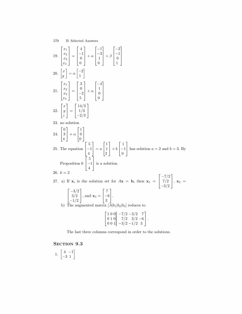
570 B Selected Answers
19.
x1
x2
x3
x4
=
4−100
+ α
−1−310
+ β
−2−101
20.
[
xy
]
= α
[
−21
]
21.
x1
x2
x3
x4
=
30−25
+ α
−4100
22.
xyz
=
14/31/3−2/3
23. no solution
24.
034
+ α
100
25. The equation
5−14
= a
112
+ b
1−10
has solution a = 2 and b = 3. By
Proposition 6
5−14
is a solution.
26. k = 2
27. a) If xi is the solution set for Ax = bi then x1 =
−7/27/2−3/2
, x2 =
−3/23/2−1/2
, and x3 =
7−63
.
b) The augmented matrix [A|b1|b2|b3] reduces to
1 0 0 −7/2 −3/2 70 1 0 7/2 3/2 −60 0 1 −3/2 −1/2 3
.
The last three columns correspond in order to the solutions.
Section 9.3
1.
[
4 −1−3 1
]
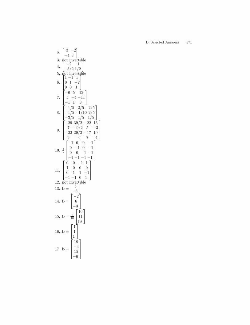
B Selected Answers 571
2.
[
3 −2−4 3
]
3. not invertible
4.
[
−2 1−3/2 1/2
]
5. not invertible
6.
1 −1 10 1 −20 0 1
7.
−6 5 135 −4 −11−1 1 3
8.
−1/5 2/5 2/5−1/5 −1/10 2/5−3/5 1/5 1/5
9.
−29 39/2 −22 137 −9/2 5 −3−22 29/2 −17 109 −6 7 −4
10. 12
−1 0 0 −10 −1 0 −10 0 −1 −1−1 −1 −1 −1
11.
0 0 −1 11 0 0 00 1 1 −1−1 −1 0 1
12. not invertible
13. b =
[
5−3
]
14. b =
−26−3
15. b = 110
161118
16. b =
111
17. b =
19−415−6
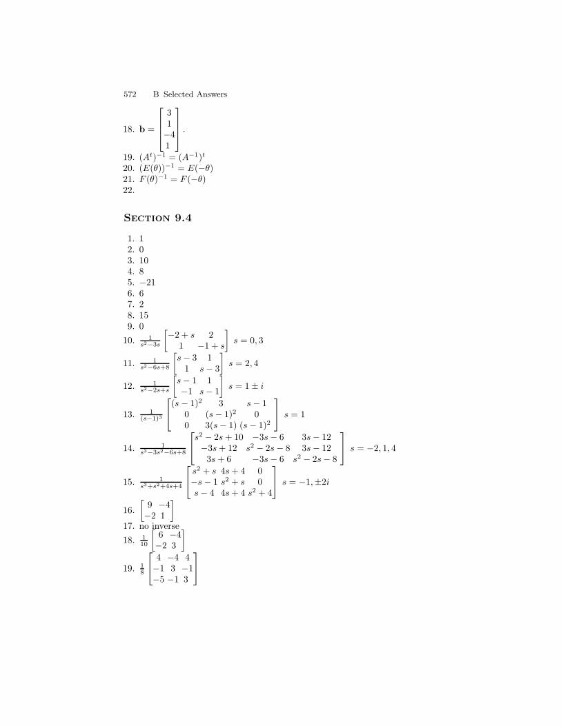
572 B Selected Answers
18. b =
31−41
.
19. (At)−1 = (A−1)t
20. (E(θ))−1 = E(−θ)21. F (θ)−1 = F (−θ)22.
Section 9.4
1. 12. 03. 104. 85. −216. 67. 28. 159. 0
10. 1s2−3s
[
−2 + s 21 −1 + s
]
s = 0, 3
11. 1s2−6s+8
[
s− 3 11 s− 3
]
s = 2, 4
12. 1s2−2s+s
[
s− 1 1−1 s− 1
]
s = 1± i
13. 1(s−1)3
(s− 1)2 3 s− 10 (s− 1)2 00 3(s− 1) (s− 1)2
s = 1
14. 1s3−3s2−6s+8
s2 − 2s+ 10 −3s− 6 3s− 12−3s+ 12 s2 − 2s− 8 3s− 123s+ 6 −3s− 6 s2 − 2s− 8
s = −2, 1, 4
15. 1s3+s2+4s+4
s2 + s 4s+ 4 0−s− 1 s2 + s 0s− 4 4s+ 4 s2 + 4
s = −1,±2i
16.
[
9 −4−2 1
]
17. no inverse
18. 110
[
6 −4−2 3
]
19. 18
4 −4 4−1 3 −1−5 −1 3
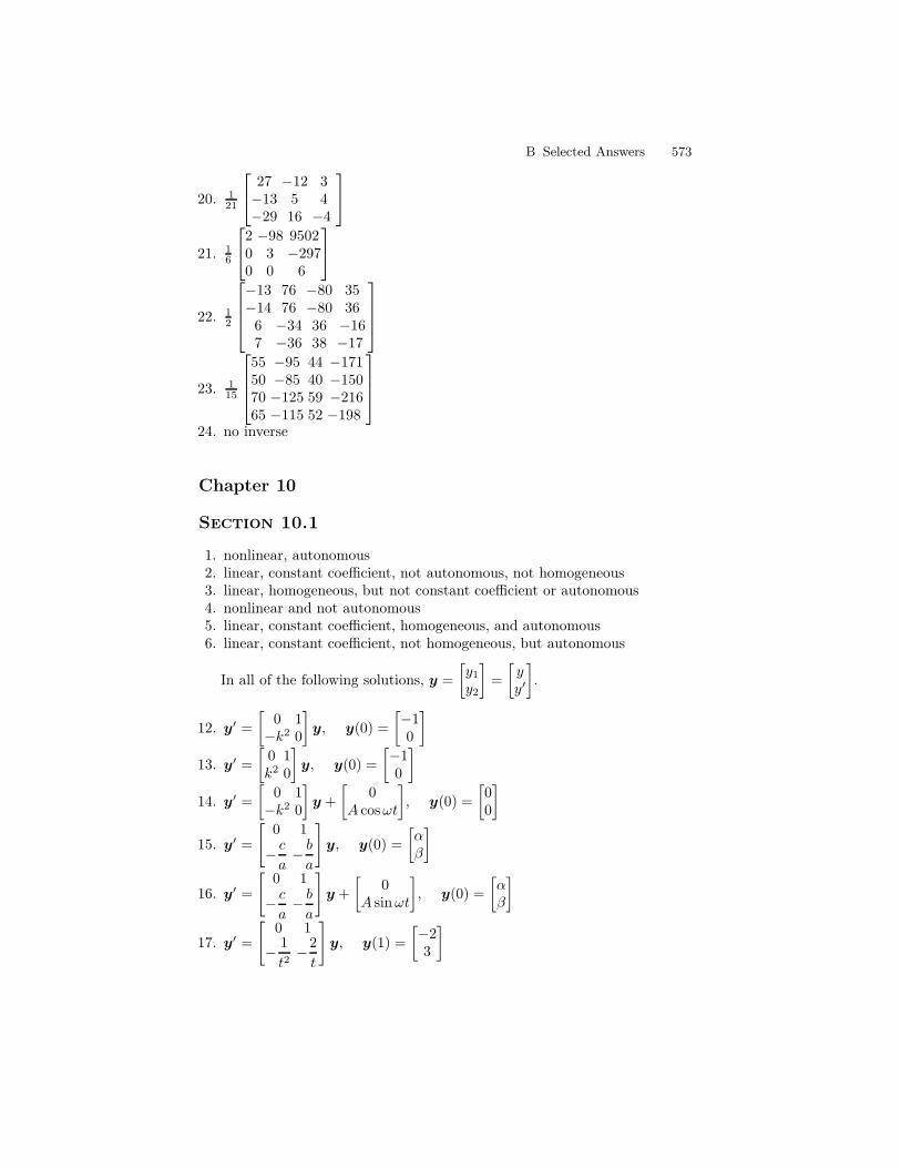
B Selected Answers 573
20. 121
27 −12 3−13 5 4−29 16 −4
21. 16
2 −98 95020 3 −2970 0 6
22. 12
−13 76 −80 35−14 76 −80 366 −34 36 −167 −36 38 −17
23. 115
55 −95 44 −17150 −85 40 −15070 −125 59 −21665 −115 52 −198
24. no inverse
Chapter 10
Section 10.1
1. nonlinear, autonomous2. linear, constant coefficient, not autonomous, not homogeneous3. linear, homogeneous, but not constant coefficient or autonomous4. nonlinear and not autonomous5. linear, constant coefficient, homogeneous, and autonomous6. linear, constant coefficient, not homogeneous, but autonomous
In all of the following solutions, y =
[
y1y2
]
=
[
yy′
]
.
12. y′ =
[
0 1−k2 0
]
y, y(0) =
[
−10
]
13. y′ =
[
0 1k2 0
]
y, y(0) =
[
−10
]
14. y′ =
[
0 1−k2 0
]
y +
[
0A cosωt
]
, y(0) =
[
00
]
15. y′ =
[
0 1
− ca− ba
]
y, y(0) =
[
αβ
]
16. y′ =
[
0 1
− ca− ba
]
y +
[
0A sinωt
]
, y(0) =
[
αβ
]
17. y′ =
[
0 1
− 1
t2−2
t
]
y, y(1) =
[
−23
]
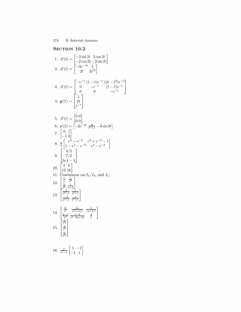
574 B Selected Answers
Section 10.2
1. A′(t) =
[
−2 sin 2t 2 cos 2t−2 cos 2t −2 sin 2t
]
2. A′(t) =
[
−3e−3t 12t 2e2t
]
3. A′(t) =
−e−t (1− t)e−t (2t− t2)e−t
0 −e−t (1 − t)e−t
0 0 −e−t
4. y′(t) =
12tt−1
5. A′(t) =
[
0 00 0
]
6. v′(t) =[
−2e−2t 2tt2+1 −3 sin3t
]
7.
[
0 1−1 0
]
8. 14
[
e2 − e−2 e2 + e−2 − 11− e2 − e−2 e2 − e−2
]
9.
3/27/3
ln 4− 1
10.
[
4 812 16
]
11. Continuous on I1, I4, and I5.
12.
[
1s
1s2
2s3
1s−2
]
13.
[
2s2+1
1s2+1
−1s2+1
ss2+1
]
14.
[
3!s4
2s(s2+1)2
1(s+1)2
2−ss3
s−3s2−6s+13
3s
]
15.
1s2
2s3
6s4
16. 2s2−1
[
1 −1−1 1
]
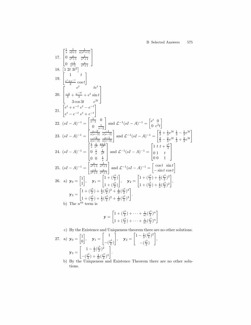
B Selected Answers 575
17.
1s
1s2+1
1s(s2+1)
0 ss2+1
1s2+1
0 −1s+1
ss2+1
18.[
1 2t 3t2]
19.
[
1 t
et+e−t
2 cos t
]
20.
et tet
−43 + e−3t
3 + et sin t
3 cos 3t e3t
21.
[
et + e−t et − e−t
et − e−t et + e−t
]
22. (sI −A)−1 =
[
1s−1 0
0 1s−2
]
and L−1(sI −A)−1 =
[
et 00 e2t
]
23. (sI −A)−1 =
[
s−2s(s−3)
−1s(s−3)
−2s(s−3)
s−1s(s−3)
]
and L−1(sI −A)−1 =
[
23 + 1
3e3t 1
3 − 13e
3t
23 − 2
3e3t 1
3 + 23e
3t
]
24. (sI −A)−1 =
1s
1s2
s+1s3
0 1s
1s2
0 0 1s
and L−1(sI −A)−1 =
1 t t+ t2
2
0 1 t0 0 1
25. (sI −A)−1 =
[
ss2+1
1s2+1
−1s2+1
ss2+1
]
and L−1(sI −A)−1 =
[
cos t sin t− sin t cos t
]
26. a) y0 =
[
11
]
, y1 =
[
1 + ( t2
2 )
1 + ( t2
2 )
]
, y2 =
[
1 + ( t2
2 ) + 12 ( t2
2 )2
1 + ( t2
2 ) + 12 ( t2
2 )2
]
,
y3 =
[
1 + ( t2
2 ) + 12 ( t2
2 )2 + 13! (
t2
2 )3
1 + ( t2
2 ) + 12 ( t2
2 )2 + 13! (
t2
2 )3
]
.
b) The nth term is
y =
[
1 + ( t2
2 ) + · · ·+ 1n! (
t2
2 )n
1 + ( t2
2 ) + · · ·+ 1n! (
t2
2 )n
]
c) By the Existence and Uniqueness theorem there are no other solutions.
27. a) y0 =
[
10
]
, y1 =
[
1
−( t2
2 )
]
, y2 =
[
1− 12 ( t2
2 )2
−( t2
2 )
]
,
y3 =
[
1− 12 ( t2
2 )2
−( t2
2 ) + 13! (
t2
2 )3
]
.
b) By the Uniqueness and Existence Theorem there are no other solu-tions.
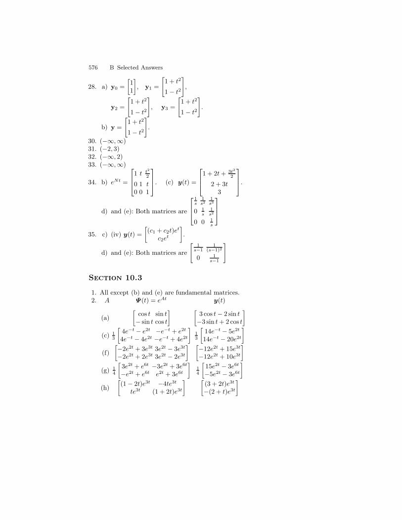
576 B Selected Answers
28. a) y0 =
[
11
]
, y1 =
[
1 + t2
1− t2
]
,
y2 =
[
1 + t2
1− t2
]
, y3 =
[
1 + t2
1− t2
]
.
b) y =
[
1 + t2
1− t2
]
.
30. (−∞,∞)31. (−2, 3)32. (−∞, 2)33. (−∞,∞)
34. b) eNt =
1 t t2
2
0 1 t0 0 1
. (c) y(t) =
1 + 2t+ 3t2
2
2 + 3t3
.
d) and (e): Both matrices are
1s
1s2
1s3
0 1s
1s2
0 0 1s
35. c) (iv) y(t) =
[
(c1 + c2t)et
c2et
]
.
d) and (e): Both matrices are
[
1s−1
1(s−1)2
0 1s−1
]
Section 10.3
1. All except (b) and (e) are fundamental matrices.2. A Ψ (t) = eAt y(t)
(a)
[
cos t sin t− sin t cos t
] [
3 cos t− 2 sin t−3 sin t+ 2 cos t
]
(c) 13
[
4e−t − e2t −e−t + e2t
4e−t − 4e2t −e−t + 4e2t
]
13
[
14e−t − 5e2t
14e−t − 20e2t
]
(f)
[
−2e2t + 3e3t 3e2t − 3e3t
−2e2t + 2e3t 3e2t − 2e3t
] [
−12e2t + 15e3t
−12e2t + 10e3t
]
(g) 14
[
3e2t + e6t −3e2t + 3e6t
−e2t + e6t e2t + 3e6t
]
14
[
15e2t − 3e6t
−5e2t − 3e6t
]
(h)
[
(1− 2t)e3t −4te3t
te3t (1 + 2t)e3t
] [
(3 + 2t)e3t
−(2 + t)e3t
]
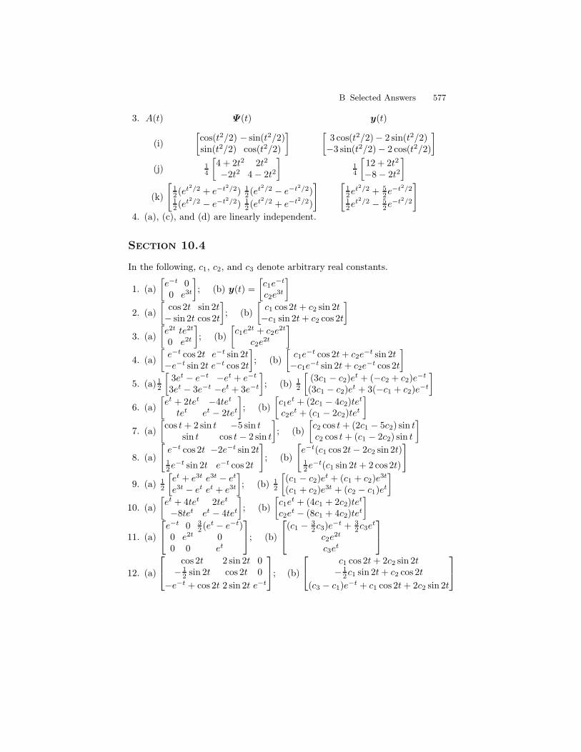
B Selected Answers 577
3. A(t) Ψ (t) y(t)
(i)
[
cos(t2/2) − sin(t2/2)sin(t2/2) cos(t2/2)
] [
3 cos(t2/2)− 2 sin(t2/2)−3 sin(t2/2)− 2 cos(t2/2)
]
(j) 14
[
4 + 2t2 2t2
−2t2 4− 2t2
]
14
[
12 + 2t2
−8− 2t2
]
(k)
[
12 (et2/2 + e−t2/2) 1
2 (et2/2 − e−t2/2)12 (et2/2 − e−t2/2) 1
2 (et2/2 + e−t2/2)
] [
12e
t2/2 + 52e
−t2/2
12e
t2/2 − 52e
−t2/2
]
4. (a), (c), and (d) are linearly independent.
Section 10.4
In the following, c1, c2, and c3 denote arbitrary real constants.
1. (a)
[
e−t 00 e3t
]
; (b) y(t) =
[
c1e−t
c2e3t
]
2. (a)
[
cos 2t sin 2t− sin 2t cos 2t
]
; (b)
[
c1 cos 2t+ c2 sin 2t−c1 sin 2t+ c2 cos 2t
]
3. (a)
[
e2t te2t
0 e2t
]
; (b)
[
c1e2t + c2e
2t
c2e2t
]
4. (a)
[
e−t cos 2t e−t sin 2t−e−t sin 2t e−t cos 2t
]
; (b)
[
c1e−t cos 2t+ c2e
−t sin 2t−c1e−t sin 2t+ c2e
−t cos 2t
]
5. (a)12
[
3et − e−t −et + e−t
3et − 3e−t −et + 3e−t
]
; (b) 12
[
(3c1 − c2)et + (−c2 + c2)e−t
(3c1 − c2)et + 3(−c1 + c2)e−t
]
6. (a)
[
et + 2tet −4tet
tet et − 2tet
]
; (b)
[
c1et + (2c1 − 4c2)te
t
c2et + (c1 − 2c2)te
t
]
7. (a)
[
cos t+ 2 sin t −5 sin tsin t cos t− 2 sin t
]
; (b)
[
c2 cos t+ (2c1 − 5c2) sin tc2 cos t+ (c1 − 2c2) sin t
]
8. (a)
[
e−t cos 2t −2e−t sin 2t
12e
−t sin 2t e−t cos 2t
]
; (b)
[
e−t(c1 cos 2t− 2c2 sin 2t)
12e
−t(c1 sin 2t+ 2 cos 2t)
]
9. (a) 12
[
et + e3t e3t − et
e3t − et et + e3t
]
; (b) 12
[
(c1 − c2)et + (c1 + c2)e3t
(c1 + c2)e3t + (c2 − c1)et
]
10. (a)
[
et + 4tet 2tet
−8tet et − 4tet
]
; (b)
[
c1et + (4c1 + 2c2)te
t
c2et − (8c1 + 4c2)te
t
]
11. (a)
e−t 0 32 (et − e−t)
0 e2t 00 0 et
; (b)
(c1 − 32c3)e
−t + 32c3e
t
c2e2t
c3et
12. (a)
cos 2t 2 sin 2t 0− 1
2 sin 2t cos 2t 0
−e−t + cos 2t 2 sin 2t e−t
; (b)
c1 cos 2t+ 2c2 sin 2t− 1
2c1 sin 2t+ c2 cos 2t
(c3 − c1)e−t + c1 cos 2t+ 2c2 sin 2t
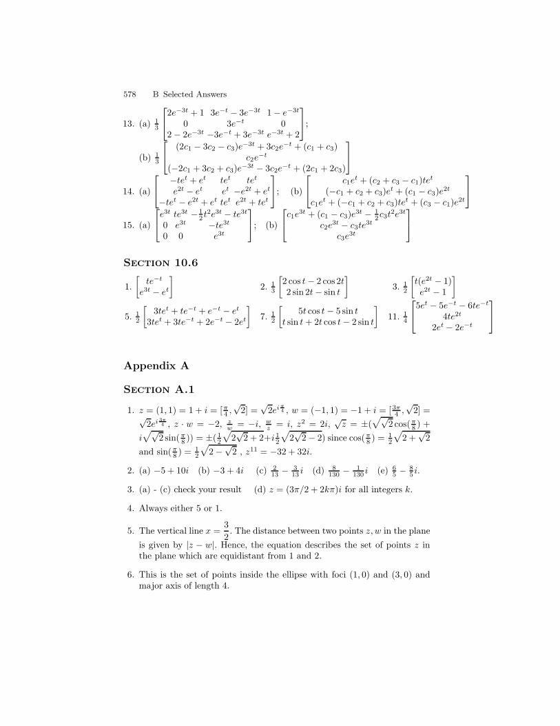
578 B Selected Answers
13. (a) 13
2e−3t + 1 3e−t − 3e−3t 1− e−3t
0 3e−t 02− 2e−3t −3e−t + 3e−3t e−3t + 2
;
(b) 13
(2c1 − 3c2 − c3)e−3t + 3c2e−t + (c1 + c3)
c2e−t
(−2c1 + 3c2 + c3)e−3t − 3c2e
−t + (2c1 + 2c3)
14. (a)
−tet + et tet tet
e2t − et et −e2t + et
−tet − e2t + et tet e2t + tet
; (b)
c1et + (c2 + c3 − c1)tet
(−c1 + c2 + c3)et + (c1 − c3)e2t
c1et + (−c1 + c2 + c3)te
t + (c3 − c1)e2t
15. (a)
e3t te3t − 12 t
2e3t − te3t
0 e3t −te3t
0 0 e3t
; (b)
c1e3t + (c1 − c3)e3t − 1
2c3t2e3t
c2e3t − c3te3t
c3e3t
Section 10.6
1.
[
te−t
e3t − et
]
2. 13
[
2 cos t− 2 cos 2t2 sin 2t− sin t
]
3. 12
[
t(e2t − 1)e2t − 1
]
5. 12
[
3tet + te−t + e−t − et
3tet + 3te−t + 2e−t − 2et
]
7. 12
[
5t cos t− 5 sin tt sin t+ 2t cos t− 2 sin t
]
11. 14
5et − 5e−t − 6te−t
4te2t
2et − 2e−t
Appendix A
Section A.1
1. z = (1, 1) = 1 + i = [π4 ,√
2] =√
2ei π4 , w = (−1, 1) = −1 + i = [3π
4 ,√
2] =√2ei 3π
4 , z · w = −2, zw = −i, w
z = i, z2 = 2i,√z = ±(
√√2 cos(π
8 ) +
i√√
2 sin(π8 )) = ±(1
2
√
2√
2 + 2+i 12
√
2√
2− 2) since cos(π8 ) = 1
2
√
2 +√
2
and sin(π8 ) = 1
2
√
2−√
2 , z11 = −32 + 32i.
2. (a) −5 + 10i (b) −3 + 4i (c) 213 − 3
13 i (d) 8130 − 1
130 i (e) 65 − 8
5 i.
3. (a) - (c) check your result (d) z = (3π/2 + 2kπ)i for all integers k.
4. Always either 5 or 1.
5. The vertical line x =3
2. The distance between two points z, w in the plane
is given by |z − w|. Hence, the equation describes the set of points z inthe plane which are equidistant from 1 and 2.
6. This is the set of points inside the ellipse with foci (1, 0) and (3, 0) andmajor axis of length 4.
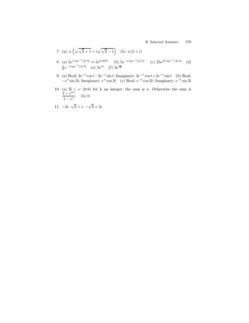
B Selected Answers 579
7. (a) ±(
√√2 + 1 + i
√√2− 1
)
(b) ±(2 + i)
8. (a) 5ei tan−1(4/3) ≈ 5e0.927i (b) 5e−i tan−1(4/3) (c) 25e2i tan−1(4/3) (d)15e
−i tan−1(4/3) (e) 5eiπ (f) 3eiπ2
9. (a) Real: 2e−t cos t−3e−t sin t; Imaginary: 3e−t cos t+2e−t sin t (b) Real:−eπ sin 2t; Imaginary: eπ cos 2t (c) Real: e−t cos 2t; Imaginary: e−t sin 2t
10. (a) If z = 2πki for k an integer, the sum is n. Otherwise the sum is1− enz
1− ez. (b) 0
11. −2i,√
3 + i, −√
3 + 2i

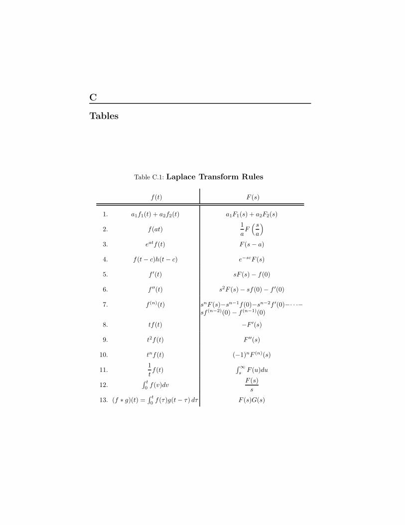
C
Tables
Table C.1: Laplace Transform Rules
f(t) F (s)
1. a1f1(t) + a2f2(t) a1F1(s) + a2F2(s)
2. f(at)1
aF( s
a
)
3. eatf(t) F (s− a)
4. f(t− c)h(t− c) e−scF (s)
5. f ′(t) sF (s)− f(0)
6. f ′′(t) s2F (s)− sf(0)− f ′(0)
7. f (n)(t) snF (s)−sn−1f(0)−sn−2f ′(0)−· · ·−sf (n−2)(0)− f (n−1)(0)
8. tf(t) −F ′(s)
9. t2f(t) F ′′(s)
10. tnf(t) (−1)nF (n)(s)
11.1
tf(t)
∫∞s F (u)du
12.∫ t
0 f(v)dvF (s)
s
13. (f ∗ g)(t) =∫ t
0f(τ)g(t− τ) dτ F (s)G(s)
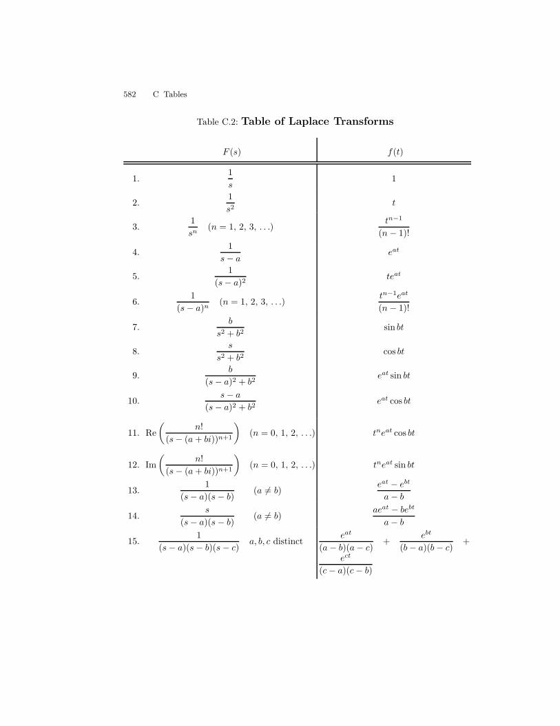
582 C Tables
Table C.2: Table of Laplace Transforms
F (s) f(t)
1.1
s1
2.1
s2t
3.1
sn(n = 1, 2, 3, . . .)
tn−1
(n− 1)!
4.1
s− a eat
5.1
(s− a)2 teat
6.1
(s− a)n(n = 1, 2, 3, . . .)
tn−1eat
(n− 1)!
7.b
s2 + b2sin bt
8.s
s2 + b2cos bt
9.b
(s− a)2 + b2eat sin bt
10.s− a
(s− a)2 + b2eat cos bt
11. Re
(
n!
(s− (a+ bi))n+1
)
(n = 0, 1, 2, . . .) tneat cos bt
12. Im
(
n!
(s− (a+ bi))n+1
)
(n = 0, 1, 2, . . .) tneat sin bt
13.1
(s− a)(s− b) (a 6= b)eat − ebt
a− b
14.s
(s− a)(s− b) (a 6= b)aeat − bebt
a− b
15.1
(s− a)(s− b)(s− c) a, b, c distincteat
(a− b)(a− c) +ebt
(b− a)(b − c) +
ect
(c− a)(c− b)
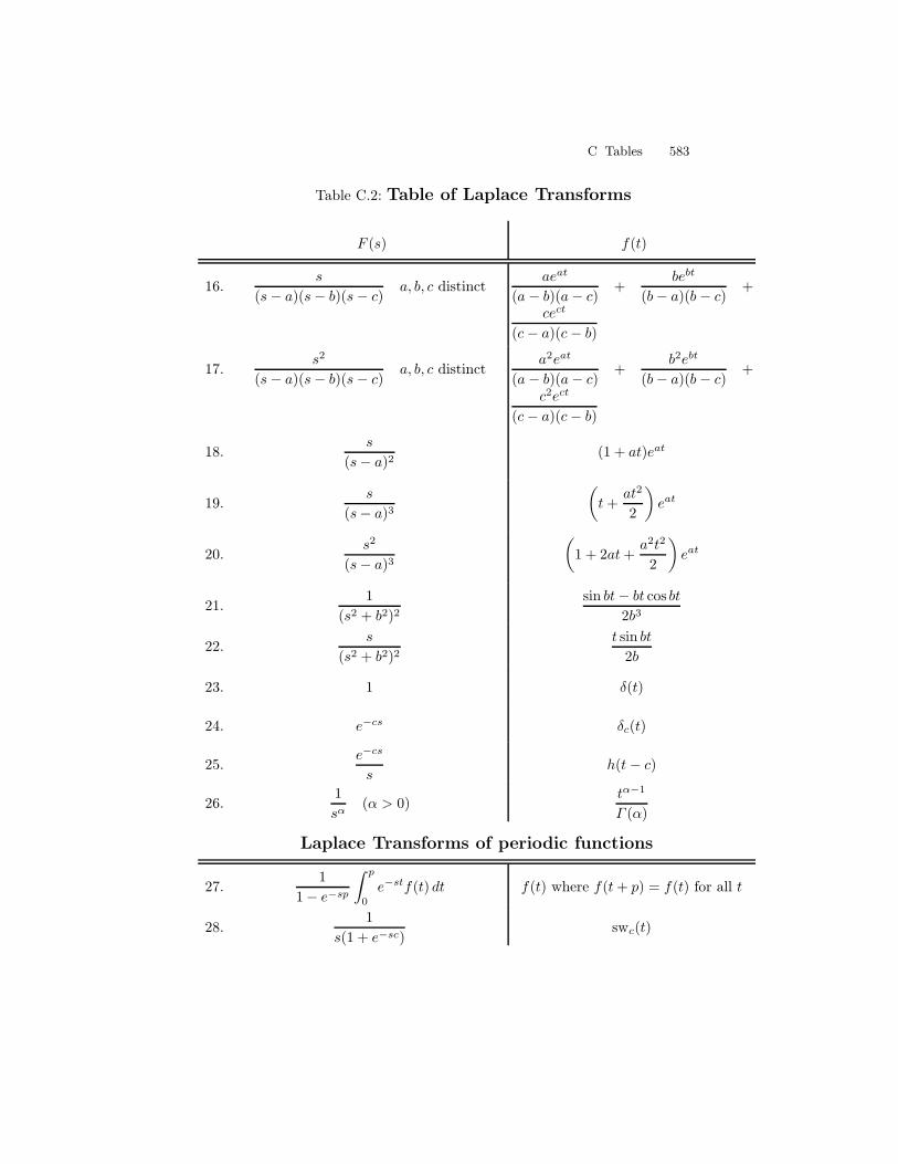
C Tables 583
Table C.2: Table of Laplace Transforms
F (s) f(t)
16.s
(s− a)(s− b)(s− c) a, b, c distinctaeat
(a− b)(a− c) +bebt
(b− a)(b − c) +
cect
(c− a)(c− b)
17.s2
(s− a)(s− b)(s− c) a, b, c distincta2eat
(a− b)(a− c) +b2ebt
(b− a)(b − c) +
c2ect
(c− a)(c− b)
18.s
(s− a)2 (1 + at)eat
19.s
(s− a)3(
t+at2
2
)
eat
20.s2
(s− a)3(
1 + 2at+a2t2
2
)
eat
21.1
(s2 + b2)2sin bt− bt cos bt
2b3
22.s
(s2 + b2)2t sin bt
2b
23. 1 δ(t)
24. e−cs δc(t)
25.e−cs
sh(t− c)
26.1
sα(α > 0)
tα−1
Γ (α)
Laplace Transforms of periodic functions
27.1
1− e−sp
∫ p
0
e−stf(t) dt f(t) where f(t+ p) = f(t) for all t
28.1
s(1 + e−sc)swc(t)
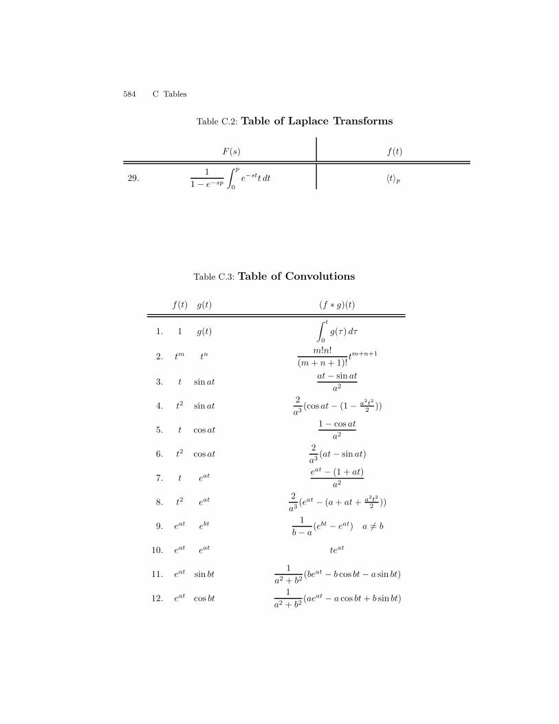
584 C Tables
Table C.2: Table of Laplace Transforms
F (s) f(t)
29.1
1− e−sp
∫ p
0
e−stt dt 〈t〉p
Table C.3: Table of Convolutions
f(t) g(t) (f ∗ g)(t)
1. 1 g(t)
∫ t
0
g(τ) dτ
2. tm tnm!n!
(m+ n+ 1)!tm+n+1
3. t sin atat− sin at
a2
4. t2 sin at2
a3(cos at− (1− a2t2
2 ))
5. t cos at1− cos at
a2
6. t2 cos at2
a3(at− sin at)
7. t eat eat − (1 + at)
a2
8. t2 eat 2
a3(eat − (a+ at+ a2t2
2 ))
9. eat ebt 1
b− a(ebt − eat) a 6= b
10. eat eat teat
11. eat sin bt1
a2 + b2(beat − b cos bt− a sin bt)
12. eat cos bt1
a2 + b2(aeat − a cos bt+ b sin bt)
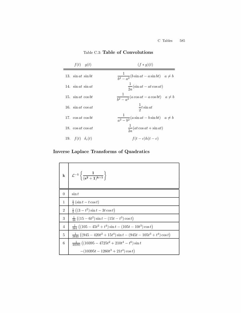
C Tables 585
Table C.3: Table of Convolutions
f(t) g(t) (f ∗ g)(t)
13. sin at sin bt1
b2 − a2(b sin at− a sin bt) a 6= b
14. sin at sin at1
2a(sin at− at cos at)
15. sin at cos bt1
b2 − a2(a cos at− a cos bt) a 6= b
16. sin at cos at1
2t sin at
17. cos at cos bt1
a2 − b2 (a sin at− b sin bt) a 6= b
18. cos at cos at1
2a(at cos at+ sin at)
19. f(t) δc(t) f(t− c)h(t− c)
Inverse Laplace Transforms of Quadratics
k L−1
1
(s2 + 1)k+1
0 sin t
1 12 (sin t− t cos t)
2 18
(
(3− t2) sin t− 3t cos t)
3 148
(
(15− 6t2) sin t− (15t− t3) cos t)
4 1384
(
(105− 45t2 + t4) sin t− (105t− 10t3) cos t)
5 13840
(
(945− 420t2 + 15t4) sin t− (945t− 105t3 + t4) cos t)
6 146080
(
(10395− 4725t2 + 210t4 − t6) sin t
−(10395t− 1260t3 + 21t4) cos t)
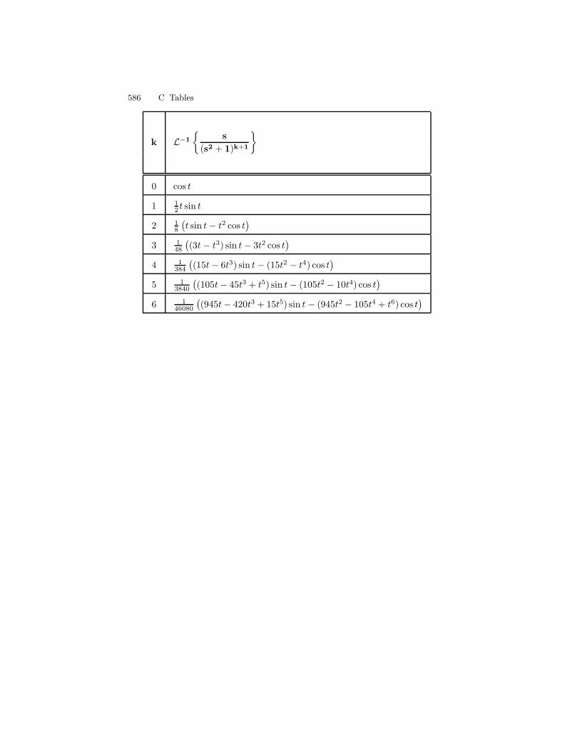
586 C Tables
k L−1
s
(s2 + 1)k+1
0 cos t
1 12 t sin t
2 18
(
t sin t− t2 cos t)
3 148
(
(3t− t3) sin t− 3t2 cos t)
4 1384
(
(15t− 6t3) sin t− (15t2 − t4) cos t)
5 13840
(
(105t− 45t3 + t5) sin t− (105t2 − 10t4) cos t)
6 146080
(
(945t− 420t3 + 15t5) sin t− (945t2 − 105t4 + t6) cos t)
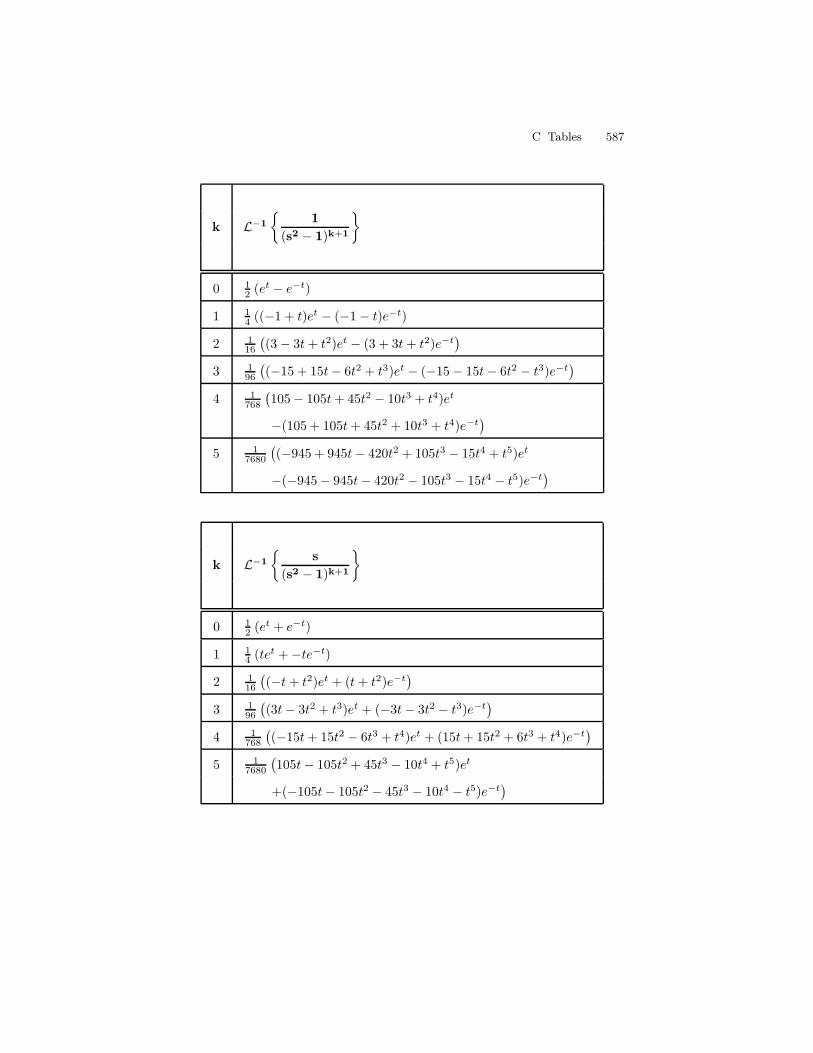
C Tables 587
k L−1
1
(s2 − 1)k+1
0 12 (et − e−t)
1 14 ((−1 + t)et − (−1− t)e−t)
2 116
(
(3 − 3t+ t2)et − (3 + 3t+ t2)e−t)
3 196
(
(−15 + 15t− 6t2 + t3)et − (−15− 15t− 6t2 − t3)e−t)
4 1768
(
105− 105t+ 45t2 − 10t3 + t4)et
−(105 + 105t+ 45t2 + 10t3 + t4)e−t)
5 17680
(
(−945 + 945t− 420t2 + 105t3 − 15t4 + t5)et
−(−945− 945t− 420t2 − 105t3 − 15t4 − t5)e−t)
k L−1
s
(s2 − 1)k+1
0 12 (et + e−t)
1 14 (tet +−te−t)
2 116
(
(−t+ t2)et + (t+ t2)e−t)
3 196
(
(3t− 3t2 + t3)et + (−3t− 3t2 − t3)e−t)
4 1768
(
(−15t+ 15t2 − 6t3 + t4)et + (15t+ 15t2 + 6t3 + t4)e−t)
5 17680
(
105t− 105t2 + 45t3 − 10t4 + t5)et
+(−105t− 105t2 − 45t3 − 10t4 − t5)e−t)

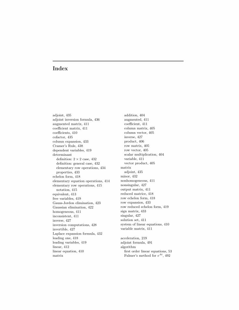
Index
adjoint, 435adjoint inversion formula, 436augmented matrix, 411coefficient matrix, 411coefficients, 410cofactor, 435column expansion, 433Cramer’s Rule, 438dependent variables, 419determinant
definition: 2 × 2 case, 432definition: general case, 432elementary row operations, 434properties, 433
echelon form, 418elementary equation operations, 414elementary row operations, 415
notation, 415equivalent, 413free variables, 419Gauss-Jordon elimination, 423Gaussian elimination, 422homogeneous, 411inconsistent, 411inverse, 427inversion computations, 428invertible, 427Laplace expansion formula, 432leading one, 418leading variables, 419linear, 412linear equation, 410matrix
addition, 404augmented, 411coefficient, 411column matrix, 405column vector, 405inverse, 427product, 406row matrix, 405row vector, 405scalar multiplication, 404variable, 411vector product, 405
matrixadjoint, 435
minor, 432nonhomogeneous, 411nonsingular, 427output matrix, 411reduced matrice, 418row echelon form, 418row expansion, 433row reduced echelon form, 419sign matrix, 433singular, 427solution set, 411system of linear equations, 410variable matrix, 411
acceleration, 219adjoint formula, 491algorithm
first order linear equations, 53Fulmer’s method for eAt, 492
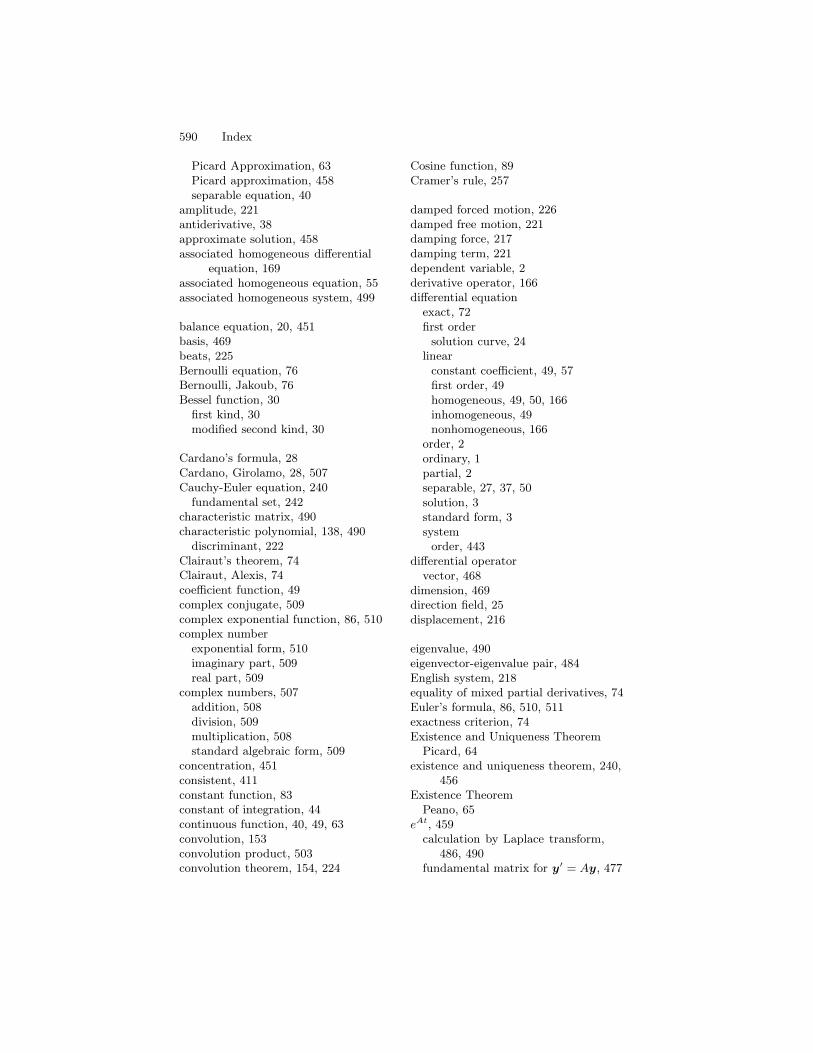
590 Index
Picard Approximation, 63Picard approximation, 458separable equation, 40
amplitude, 221antiderivative, 38approximate solution, 458associated homogeneous differential
equation, 169associated homogeneous equation, 55associated homogeneous system, 499
balance equation, 20, 451basis, 469beats, 225Bernoulli equation, 76Bernoulli, Jakoub, 76Bessel function, 30
first kind, 30modified second kind, 30
Cardano’s formula, 28Cardano, Girolamo, 28, 507Cauchy-Euler equation, 240
fundamental set, 242characteristic matrix, 490characteristic polynomial, 138, 490
discriminant, 222Clairaut’s theorem, 74Clairaut, Alexis, 74coefficient function, 49complex conjugate, 509complex exponential function, 86, 510complex number
exponential form, 510imaginary part, 509real part, 509
complex numbers, 507addition, 508division, 509multiplication, 508standard algebraic form, 509
concentration, 451consistent, 411constant function, 83constant of integration, 44continuous function, 40, 49, 63convolution, 153convolution product, 503convolution theorem, 154, 224
Cosine function, 89Cramer’s rule, 257
damped forced motion, 226damped free motion, 221damping force, 217damping term, 221dependent variable, 2derivative operator, 166differential equation
exact, 72first order
solution curve, 24linear
constant coefficient, 49, 57first order, 49homogeneous, 49, 50, 166inhomogeneous, 49nonhomogeneous, 166
order, 2ordinary, 1partial, 2separable, 27, 37, 50solution, 3standard form, 3system
order, 443differential operator
vector, 468dimension, 469direction field, 25displacement, 216
eigenvalue, 490eigenvector-eigenvalue pair, 484English system, 218equality of mixed partial derivatives, 74Euler’s formula, 86, 510, 511exactness criterion, 74Existence and Uniqueness Theorem
Picard, 64existence and uniqueness theorem, 240,
456Existence Theorem
Peano, 65eAt, 459
calculation by Laplace transform,486, 490
fundamental matrix for y′ = Ay, 477
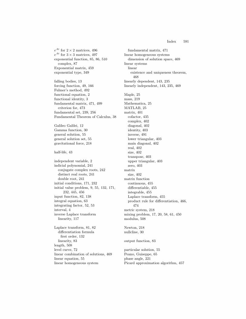
Index 591
eAt for 2 × 2 matrices, 496eAt for 3 × 3 matrices, 497exponential function, 85, 86, 510
complex, 87Exponential matrix, 459exponential type, 349
falling bodies, 13forcing function, 49, 166Fulmer’s method, 492functional equation, 2functional identity, 3fundamental matrix, 471, 499
criterion for, 473fundamental set, 239, 256Fundamental Theorem of Calculus, 38
Galileo Galilei, 12Gamma function, 30general solution, 55general solution set, 55gravitational force, 218
half-life, 43
independent variable, 2indicial polynomial, 241
conjugate complex roots, 242distinct real roots, 241double root, 241
initial conditions, 171, 232initial value problem, 9, 55, 132, 171,
232, 445, 456input function, 82, 138integral equation, 63integrating factor, 52, 53interval, 4inverse Laplace transform
linearity, 117
Laplace transform, 81, 82differentiation formula
first order, 132linearity, 83
length, 508level curve, 72linear combination of solutions, 469linear equation, 55linear homogeneous system
fundamental matrix, 471linear homogeneous systems
dimension of solution space, 469linear systems
linearexistence and uniqueness theorem,
468linearly dependent, 143, 235linearly independent, 143, 235, 469
Maple, 25mass, 219Mathematica, 25MATLAB, 25matrix, 401
cofactor, 435complex, 402diagonal, 402identity, 403inverse, 491lower triangular, 403main diagonal, 402real, 402size, 402transpose, 403upper triangular, 403zero, 403
matrixsize, 402
matrix functioncontinuous, 455differentiable, 455integrable, 455Laplace transform, 455product rule for differentiation, 466,
474metric system, 218mixing problem, 17, 20, 58, 61, 450modulus, 508
Newton, 218nullcline, 30
output function, 83
particular solution, 55Peano, Guiseppe, 65phase angle, 221Picard approximation algorithm, 457
592 Index
Picard, Émile, 63polar coordinates, 508power function, 84predator-prey system, 449proper rational function, 491
radioactive decay, 43radius, 508rate in − rate out, 20Rate in - Rate out, 451rate of change, 20, 43real numbers, 508restoring force, 216Ricatti equation, 30Riccati equation, 65
Sine function, 89slope field, 24slug, 218solution, 411
constant, 45steady state solution, 226successive approximations, 62system of constant coefficient linear
differential equationssolution by Laplace transform, 480
system of differential equationsfirst order
autonomous, 447constant coefficient linear, 447linear, 447, 454linear and homogeneous, 447
solution, 445standard form, 445
linear constant coefficientexponential solution, 460
linear homogeneous, 468linear nonhomogeneous, 499
associated homogeneous system,499
system of ordinary differentialequations, 443
Taylor series expansion, 459transform function, 83transient solution, 226
undamped forced motion, 223undamped free motion, 220uniqueness
geometric meaning, 69units of measurement, 218
variation of parameters, 256, 501vector space, 55, 469
basis, 469dimension, 469
Verhulst population equation, 44
Wronskian, 238Wronskian matrix, 237, 257
zero-input solution, 138zero-state solution, 138