NONLINEAR OBSERVER TECHNIQUESFOR OSCILLATORY FAILURE CASE DETECTION

D. E¦mov1 and A. Zolghadri2

1INRIA ¡ LNEParc Scienti¦que de la Haute Borne

40 Avenue Halley, B�at. A Park Plaza, Villeneuve d£Ascq 59650, France2University of Bordeaux, IMS-lab, Automatic Control Group

351 Cours de la Lib‚eration, Talence 33405, France

The problem of observer design for fault detection in a class of nonlin-ear systems subject to parametric and signal uncertainties is studied.The design procedure includes formalized optimization of observer freeparameters in terms of trade-o¨s for fault detection performance and ro-bustness to external disturbances or model uncertainties. The techniquemakes use of some monotonicity conditions imposed on the estimationerror dynamics. E©ciency of the proposed approach is demonstratedthrough the Oscillatory Failure Case (OFC) in aircraft control surfaceservoloops.

1 INTRODUCTION

Model-based Fault Detection and Isolation (FDI) in dynamical systems is anactive research area (for a recent survey, see [1,2]). An important focus has beenmade on the use of observer-based schemes. In the linear case, it has been shownthat any linear fault detection ¦lter can be transformed into an observer-basedform [3], providing a uni¦ed framework for analysis and implementation [4 8].From an estimation point of view, the problem of optimal noise ¦ltering forstochastic linear systems has many solutions [9, 10]. For nonlinear systems, ageneral framework does not exist, although numerical or suboptimal solutionsare available [11 13]. Typically, the observer design problem is solvable for acanonical representation of nonlinear systems [14,15].In this paper, an approach is developed for nonlinear fault detection observer

design, together with a procedure for parameter tuning. For the latter, the designis made under monotonicity assumption [16] for the estimation error dynamic.

Progress in Flight Dynamics, GNC, and Avionics 6 (2013) 375-392 DOI: 10.1051/eucass/201306375 © Owned by the authors, published by EDP Sciences, 2013

This is an Open Access article distributed under the terms of the Creative Commons Attribution License 2.0, which permits unrestricted use, distribution, and reproduction in any medium, provided the original work is properly cited.

Article available at http://www.eucass-proceedings.eu or http://dx.doi.org/10.1051/eucass/201306375

PROGRESS IN FLIGHT DYNAMICS, GNC, AND AVIONICS

In this case, using an appropriate linear parameter varying (LPV) transforma-tion [17 19], the design of minorant and majorant monotone linear systems ispossible, whose solutions create an envelope for the original system trajectories.Solving an optimization problem for the minorant and majorant systems (thesolution is straightforward due to their linearity), it is possible to obtain a sub-optimal solution for the original nonlinear system (a local optimality is ensuredwhen the system solutions converge to the minorant or majorant §ows). Thegoal is to maximize robustness with respect to disturbances and sensitivity withrespect to faults.In some cases, the faulty signal is known to belong to a speci¦c class of

signals (e. g., the harmonic functions of time with prede¦ned frequency range).For example, in the ODC detection considered in [20], the faults are assumed tobe harmonic. Such a priori available information simpli¦es searched solution,since speci¦ed techniques oriented on analysis of the harmonic input responsecan be used for design of observer gains.The following nonlinear system is considered:

‘x = Ax+GF(Hx,u+ f , θ) + Sv ; y = Cx+ d (1)

where x ∈ Rn, u ∈ R

m, and y ∈ Rp are the system state, input, and output;

v ∈ Rv and d ∈ R

p are the state and the output disturbances; f ∈ Rm is the

faulty signal (unknown portion of the input); θ ∈ Rq is the vector of unknown

parameters; the matrices A, G, H, S, and C are known and constant havingappropriate dimensions; and the function F : R

l+m+q → Rg is continuously

di¨erentiable. The matrices G and H are introduced to take into account moreaccurately the in§uence of nonlinearity on the system behavior. For simplicityof presentation, the signal f is considered to act on the control signal as additivedisturbance. Such a restriction is motivated by the numerical example studyfrom aeronautic ¦eld in section 6. However, the approach can be applied tomultiplicative faults also. Assume that all input signals u, f, v, and d are(Lebesgue) measurable and essentially bounded, i. e.,

‖ f ‖ ess supt≥0|f(t)| < +∞ .

The objective is to design an observer for (1) using the available noisy mea-surements y and the input u, and ensuring robustness with respect to the un-certain parameters θ and the signals v and d. Moreover, for fault detection, it isrequired to ¦nd the observer gains maximizing sensitivity of the output estima-tion error with respect to f and robustness with respect to v and d. Note thatif the fault detection problem is not of interest, then f can be considered as anadditional unknown input.Two solutions of this problem are presented below. One is more conventional

and it is based on LMIs veri¦cation (see section 4). It is shown that optimization

376

FAULT DETECTION AND CONTROL

in this framework is complicated. Another solution is the main contribution ofthe work, and it utilizes the monotone system routine for analysis and optimiza-tion (see section 5).The paper is organized as follows. Preliminaries are given in section 2. The

observer equations are introduced in section 3. Stability conditions based onLMIs are presented in section 4 (the optimization possibilities of this approachare also discussed). An alternative approach (monotone system theory) for theobserver stability analysis and the new optimization technique are given in sec-tion 5. In section 6, the overall approach is illustrated through its application toOFC detection in aircraft control surface servoloops.

2 PRELIMINARIES

This section introduces some basic notions about monotone systems and LPVrepresentation of nonlinearities.

2.1 Linear Parameter Varying Representation of NonlinearFunctions

For any two vectors p and p′ of the same dimension, let de¦ne

L(p,p′) = {λp+ (1 − λ)p′ , 0 ≤ λ ≤ 1}(the line connecting the points p and p′). Since the vector valued function Fin (1) is continuously di¨erentiable, then according to the Mean Value Theorem,for any h,h′ ∈ HX , u,u′ ∈ U ∪ F , θ,θ′ ∈ Ÿ, there exist ηhj ∈ L(h,h′), ηuj∈ L(u,u′), ηθj ∈ L(θ,θ′), j = 1, g such that

F(h,u,θ)− F(h′,u′,θ′) = –x(h− h′) + –u(u− u′) + –θ(θ − θ′) ;

–x,j =∂Fj(ξ,v,q)

∂ξ

∣∣∣∣∣ξ=ηx

j ,v=ηuj ,q=ηθ

j

; –u,j =∂Fj(ξ,v,q)

∂v

∣∣∣∣∣ξ=ηx

j ,v=ηuj ,q=ηθ

j

;

–θ,j =∂F(ξ,v,q)

∂q

∣∣∣∣∣ξ=ηx

j ,v=ηuj ,q=ηθ

j

, j = 1, g

where the symbols –x,j, –u,j , –θ,j denote the jth row of the correspondingmatrix.The application of this technique gives an exact equivalent LPV represen-

tation of a nonlinear function. It is not a linearization around a single point(or around a trajectory) since the above expression is an equality. The LPV

377

PROGRESS IN FLIGHT DYNAMICS, GNC, AND AVIONICS

approach allows to transform nonlinear models to the linear ones depending onunknown parameters –x, –u, and –θ. Therefore, the complexity of the nonlin-ear model (1) can be replaced with enlarged parametric uncertainty of a linearone. This tool will be applied in the next section to analyze the estimation errordynamics of the observer.

2.2 Monotone System Theory

The system‘x = f(t,x) , x ∈ X , t ≥ 0 ,

with the solution x(t,x0) for the initial condition x(0) = x0 is called monotone,if x0 ≤ ξ0 ⇒ x(t,x0) ≤ x(t, ξ0) for all t ≥ 0 [16] (for the vectors x0 and ξ0, theinequality x0 ≤ ξ0 is understood elementwise). The system is called cooperativeif ∂fi(t,x)/∂xj ≥ 0 for all 1 ≤ i �= j ≤ n, t ∈ R and x ∈ X [16]. Cooperativesystems form a subclass of monotone ones. A matrix A with dimension n × nis called Metzler if Ai,j ≥ 0 for all 1 ≤ i �= j ≤ n. Note that for the cooperativestable system (the matrix A is Metzler and Hurwitz),

‘s(t) = As(t) + r(t) , s ∈ Rn , r ∈ Rn , t ≤ 0 ,the properties s(0) ≥ 0, r(t) ≥ 0 for all t ≥ 0 imply s(t) ≥ 0 for t ≥ 0 and,conversely, s(0) ≤ 0, r(t) ≤ 0 for all t ≥ 0 ensures s(t) ≤ 0 for t ≥ 0. The systemis called competitive if ∂fi(t,x)/∂xj ≤ 0 for all 1 ≤ i �= j ≤ n, t ∈ R and x ∈ X ;in backward time, the competitive systems behave like the cooperative ones [16].

3 ROBUST OBSERVER EQUATIONS

This section is based on the following assumption.

Assumption 1. Let the compact sets X ⊂ Rn, U ⊂ R

m, F ⊂ Rm, V ⊂ R

v,D ⊂ R

p, and Ÿ ⊂ Rq be given such that for almost all t ≥ 0,

x(t) ∈ X ; u(t) ∈ U ; f(t) ∈ F ; v(t) ∈ V ; d(t) ∈ D ; θ ∈ Ÿ .

Such constraints are rather common in nonlinear observer design theory stat-ing that the system (1) has bounded inputs and the state with some known upperbounds.Consider the following Luenberger type observer for (1):

‘z = Z(z,y,u) = Az

+GF[Hz+ L2(y −Cz),u+ L3(y −Cz), θ∗ + L4(y −Cz)] + L1(y −Cz) (2)

378

FAULT DETECTION AND CONTROL

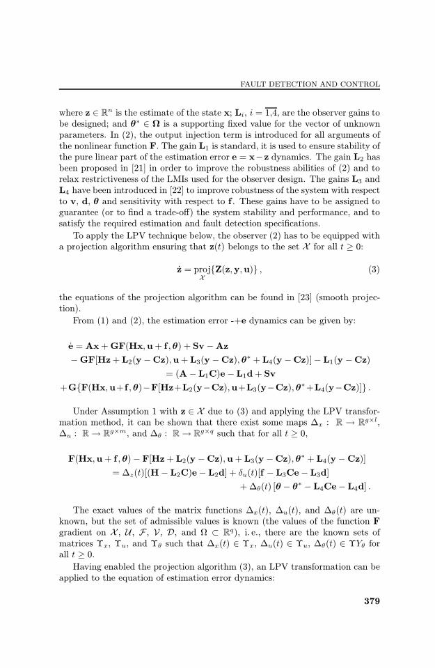
where z ∈ Rn is the estimate of the state x; Li, i = 1,4, are the observer gains to

be designed; and θ∗ ∈ Ÿ is a supporting ¦xed value for the vector of unknownparameters. In (2), the output injection term is introduced for all arguments ofthe nonlinear function F. The gain L1 is standard, it is used to ensure stability ofthe pure linear part of the estimation error e = x−z dynamics. The gain L2 hasbeen proposed in [21] in order to improve the robustness abilities of (2) and torelax restrictiveness of the LMIs used for the observer design. The gains L3 andL4 have been introduced in [22] to improve robustness of the system with respectto v, d, θ and sensitivity with respect to f . These gains have to be assigned toguarantee (or to ¦nd a trade-o¨) the system stability and performance, and tosatisfy the required estimation and fault detection speci¦cations.To apply the LPV technique below, the observer (2) has to be equipped with

a projection algorithm ensuring that z(t) belongs to the set X for all t ≥ 0:

‘z = projX{Z(z,y,u)} , (3)

the equations of the projection algorithm can be found in [23] (smooth projec-tion).From (1) and (2), the estimation error -+e dynamics can be given by:

‘e = Ax+GF(Hx,u+ f ,θ) + Sv −Az−GF[Hz+ L2(y −Cz),u+ L3(y −Cz),θ∗ + L4(y −Cz)]− L1(y −Cz)

= (A− L1C)e− L1d+ Sv+G{F(Hx,u+ f ,θ)−F[Hz+L2(y−Cz),u+L3(y−Cz),θ∗+L4(y−Cz)]} .

Under Assumption 1 with z ∈ X due to (3) and applying the LPV transfor-mation method, it can be shown that there exist some maps –x : R → R

g×l,–u : R→ R

g×m, and –θ : R→ Rg×q such that for all t ≥ 0,

F(Hx,u+ f ,θ)− F[Hz+ L2(y −Cz),u+ L3(y −Cz),θ∗ + L4(y −Cz)]= –z(t)[(H− L2C)e− L2d] + δu(t)[f − L3Ce− L3d]

+ –θ(t) [θ − θ∗ − L4Ce− L4d] .

The exact values of the matrix functions –x(t), –u(t), and –θ(t) are un-known, but the set of admissible values is known (the values of the function Fgradient on X , U , F , V , D, and Ÿ ⊂ R

q), i. e., there are the known sets ofmatrices œx, œu, and œθ such that –x(t) ∈ œx, –u(t) ∈ œu, –θ(t) ∈ œYθ forall t ≥ 0.Having enabled the projection algorithm (3), an LPV transformation can be

applied to the equation of estimation error dynamics:

379

PROGRESS IN FLIGHT DYNAMICS, GNC, AND AVIONICS

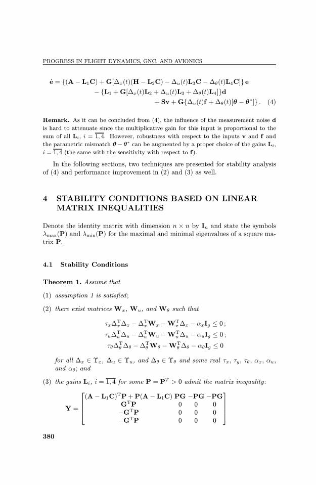
‘e = {(A− L1C) +G[–x(t)(H− L2C)−–u(t)L3C−–θ(t)L4C]} e− {L1 +G[–x(t)L2 +–u(t)L3 +–θ(t)L4]}d

+ Sv +G{–u(t)f +–θ(t)[θ − θ∗]} . (4)

Remark. As it can be concluded from (4), the in§uence of the measurement noise dis hard to attenuate since the multiplicative gain for this input is proportional to thesum of all Li, i = 1, 4. However, robustness with respect to the inputs v and f andthe parametric mismatch θ− θ∗ can be augmented by a proper choice of the gains Li,i = 1, 4 (the same with the sensitivity with respect to f).

In the following sections, two techniques are presented for stability analysisof (4) and performance improvement in (2) and (3) as well.

4 STABILITY CONDITIONS BASED ON LINEARMATRIX INEQUALITIES

Denote the identity matrix with dimension n × n by In and state the symbolsλmax(P) and λmin(P) for the maximal and minimal eigenvalues of a square ma-trix P.

4.1 Stability Conditions

Theorem 1. Assume that

(1) assumption 1 is satis¦ed ;

(2) there exist matrices Wx,Wu, and Wθ such that

τx–Tx–x −–TxWx −WTx–x − αxIg ≤ 0 ;

τu–Tu–u −–TuWu −WTu–u − αuIg ≤ 0 ;

τθ–Tθ–θ −–TθWθ −WTθ–θ − αθIg ≤ 0

for all –x ∈ œx, –u ∈ œu, and –θ ∈ œθ and some real τx, τy , τθ, αx, αu,and αθ; and

(3) the gains Li, i = 1, 4 for some P = PT > 0 admit the matrix inequality:

Y =

⎡

⎢⎢⎣

(A− L1C)TP+P(A − L1C) PG −PG −PGGTP 0 0 0−GTP 0 0 0−GTP 0 0 0

⎤

⎥⎥⎦

380

FAULT DETECTION AND CONTROL

≤

⎡

⎢⎢⎣

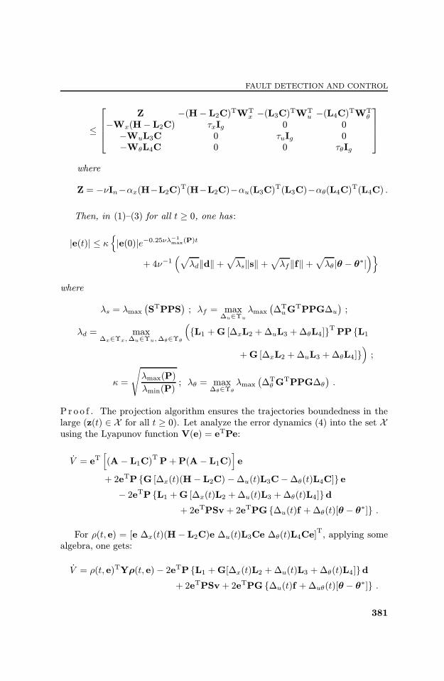
Z −(H− L2C)TWTx −(L3C)TWT

u −(L4C)TWTθ

−Wx(H− L2C) τxIg 0 0−WuL3C 0 τuIg 0−WθL4C 0 0 τθIg

⎤

⎥⎥⎦

where

Z = −νIn−αx(H−L2C)T(H−L2C)−αu(L3C)T(L3C)−αθ(L4C)T(L4C) .

Then, in (1) (3) for all t ≥ 0, one has :

|e(t)| ≤ κ{|e(0)|e−0.25νλ−1max(P)t

+ 4ν−1(√

λd‖d‖+√λs‖s‖+

√λf‖f‖+

√λθ|θ − θ∗|

)}

where

λs = λmax(STPPS

); λf = max

–u∈œu

λmax(–TuG

TPPG–u);

λd = max–x∈œx,–u∈œu,–θ∈œθ

({L1 +G [–xL2 +–uL3 +–θL4]}TPP {L1

+G [–xL2 +–uL3 +–θL4]});

κ =

√λmax(P)λmin(P)

; λθ = max–θ∈œθ

λmax(–TθG

TPPG–θ).

P r o o f . The projection algorithm ensures the trajectories boundedness in thelarge (z(t) ∈ X for all t ≥ 0). Let analyze the error dynamics (4) into the set Xusing the Lyapunov function V(e) = eTPe:

‘V = eT[(A− L1C)TP+P(A− L1C)

]e

+ 2eTP {G [–x(t)(H− L2C)−–u(t)L3C−–θ(t)L4C]} e− 2eTP {L1 +G [–x(t)L2 +–u(t)L3 +–θ(t)L4]}d

+ 2eTPSv + 2eTPG {–u(t)f +–θ(t)[θ − θ∗]} .

For ρ(t, e) = [e –x(t)(H− L2C)e –u(t)L3Ce –θ(t)L4Ce]T, applying somealgebra, one gets:

‘V = ρ(t, e)TYρ(t, e)− 2eTP {L1 +G[–x(t)L2 +–u(t)L3 +–θ(t)L4]}d+ 2eTPSv + 2eTPG {–u(t)f +–uθ(t)[θ − θ∗]} .

381

PROGRESS IN FLIGHT DYNAMICS, GNC, AND AVIONICS

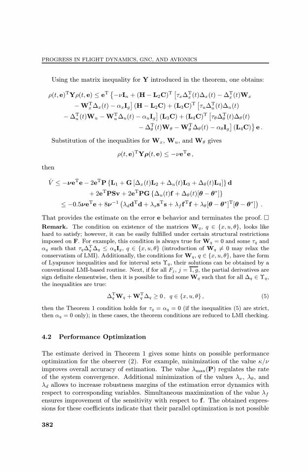
Using the matrix inequality for Y introduced in the theorem, one obtains:

ρ(t, e)TYρ(t, e) ≤ eT {−νIn + (H− L2C)T[τx–Tx (t)–x(t)−–Tx (t)Wx

−WTx–x(t)− αxIg

](H− L2C) + (L3C)T

[τu–Tu (t)–u(t)

−–Tu (t)Wu −WTu–u(t)− αuIg

](L3C) + (L4C)T

[τθ–Tθ (t)–θ(t)

−–Tθ (t)Wθ −WTθ –θ(t)− αθIg

](L4C)

}e .

Substitution of the inequalities forWx,Wu, andWθ gives

ρ(t, e)TYρ(t, e) ≤ −νeTe ,then

‘V ≤ −νeTe− 2eTP {L1 +G [–x(t)L2 +–u(t)L3 +–θ(t)L4]}d+ 2eTPSv + 2eTPG {–u(t)f +–θ(t)[θ − θ∗]}

≤ −0.5νeTe+ 8ν−1 (λddTd+ λssTs+ λf fTf + λθ[θ − θ∗]T[θ − θ∗]).

That provides the estimate on the error e behavior and terminates the proof. �Remark. The condition on existence of the matrices Wq, q ∈ {x, u, θ}, looks likehard to satisfy; however, it can be easily ful¦lled under certain structural restrictionsimposed on F. For example, this condition is always true forWq = 0 and some τq andαq such that τq–Tq –q ≤ αqIg , q ∈ {x, u, θ} (introduction of Wq �= 0 may relax theconservatism of LMI). Additionally, the conditions forWq, q ∈ {x, u, θ}, have the formof Lyapunov inequalities and for interval sets œq, their solutions can be obtained by aconventional LMI-based routine. Next, if for all Fj , j = 1, g, the partial derivatives aresign de¦nite elementwise, then it is possible to ¦nd someWq such that for all –q ∈ œq,the inequalities are true:

–TqWq +WTq –q ≥ 0 , q ∈ {x, u, θ} , (5)

then the Theorem 1 condition holds for τq = αq = 0 (if the inequalities (5) are strict,then αq = 0 only); in these cases, the theorem conditions are reduced to LMI checking.

4.2 Performance Optimization

The estimate derived in Theorem 1 gives some hints on possible performanceoptimization for the observer (2). For example, minimization of the value κ/νimproves overall accuracy of estimation. The value λmax(P) regulates the rateof the system convergence. Additional minimization of the values λν , λθ, andλd allows to increase robustness margins of the estimation error dynamics withrespect to corresponding variables. Simultaneous maximization of the value λfensures improvement of the sensitivity with respect to f . The obtained expres-sions for these coe©cients indicate that their parallel optimization is not possible

382

FAULT DETECTION AND CONTROL

and a trade-o¨ has to be found. Since such optimization is based on an upperestimate tuning, it does not provide an optimal solution (the conversation isabout a suboptimal one).The above discussion on the coe©cients λν , λθ, λf , and λd optimization

reveals that it is rather hard to optimize robustness of the system with respectto all variables v, θ, and d with simultaneous improvement of sensitivity withrespect to the faults f . Additionally, such an adjustment needs application ofthe nonlinear optimization routine. In the following section, the focus will beon particular cases (robustness with respect to v or sensitivity to harmonicsignals f).

5 MONOTONE SYSTEM APPROACH

Another approach for stability analysis and performance optimization is based onthe system (4) reduction to linear majorant and minorant systems using mono-tone system techniques, with posterior solution of the optimization problem forthese linear simpli¦ed systems. To apply the monotone systems theory, rewriteEq. (4):

‘e = “A(t)e+w(t) (6)

where

“A(t) = (A− L1C) +G[–x(t)(H− L2C)−–u(t)L3C−–θ(t)L4C] ;w(t) = −{L1 +G[–x(t)L2 +–u(t)L3 +–θ(t)L4]}d(t)

+ Sv(t) +G {–u(t)f(t) + –θ(t)[θ − θ∗]} .

Under Assumption 1, the signal w is bounded (‖w‖ < +∞)) as well as thematrix function of time “A.

Assumption 2. Let the matrix (A−L1C)+G[–x(H−L2C)−–uL3C−–θL4C]be Metzler for all –x ∈ œx, –u ∈ œu, and –θ ∈ œθ, all elements of C have thesame sign.

Assumption 2 means that the system (6) is monotone and the above men-tioned theory can be applied to their analysis and optimization. This assumptioncan be relaxed assuming existence of a linear transformation e = Xε, such thatin the new coordinates ε, the matrix X−1 “A(t)X be Metzler for all –x ∈ œx,–u ∈ œu, and –θ ∈ œθ. This relaxation is technical and skipped here forbrevity of presentation. The matrix C has positive elements in a conventionalcase C = [1 0 . . . 0]; thus, this condition is also a question of coordinate trans-formation.

383

PROGRESS IN FLIGHT DYNAMICS, GNC, AND AVIONICS

5.1 Stability Conditions

Theorem 2. Let Assumptions 1 and 2 hold. Let the gains Li, i = 1, 4 be chosento satisfy the elementwise constraint

(A− L1C) +G[–x(H− L2C)−–uL3C−–θL4C] ≤ Afor all –x ∈ œx, –u ∈ œu, and –θ ∈ œθ, where A = (A − L1C) +G[–x(H− L2C) − –uL3C − –θL4C] is Metzler and Hurwitz for some matrices –k,k ∈ {x, u, θ}.Then, in (1) and (2), the estimation error e stays bounded for all t ≥ 0.

P r o o f . Introduce the following auxiliary dynamical systems (they will be usedfor analysis purposes only):

‘er = Aer +wr(t) , r ∈ {m,M} , −∞ < wm(t) ≤ wM (t) < +∞ ,

wm(t) ≤ 0 ≤ wM (t) , (7)for all t ≥ 0, where er ∈ R

n, r ∈ {m,M}, and the initial conditions are em(0)≤ e(0) ≤ eM (0), em(0) ≤ 0 ≤ eM (0) (all vector inequalities are understoodelementwise). Since the matrix A is Hurwitz and ‖wr‖ < +∞, r ∈ {m,M},the variables er, r ∈ {m,M}, are bounded for all t ≥ 0. Moreover, eM (t) ≥ 0,em(t) ≤ 0 for all t ≥ 0 for Metzler matrix A and sign de¦nite initial conditionsand input signals wr, r ∈ {m,M}. De¦ne two relative errors εM = eM − e andεm = e− em, then

‘εM = AeM − “A(t)e+wM (t)−w(t)= “A(t)εM + [A− “A(t)]eM + [wM (t)−w(t)] ;

‘εm = “A(t)e−Aem +w(t) −wm(t)= “A(t)εm + [ “A(t)−A]em + [w(t) −wm(t)] .

By Assumption 2, the matrix “A(t) is Metzler for all t ≥ 0 and the signals[A− “A(t)]eM + [wM (t)−w(t)], [ “A(t)−A]em+ [w(t)−wm(t)] are elementwisepositive for all t ≥ 0; therefore, the variables εM (t) and εm(t) are also positivefor all t ≥ 0 since εM (0) ≥ 0 and εm(0) ≥ 0. Indeed, if there exists a coordinateεri (t), i ∈ {1, n}, r ∈ {m,M}, approaching zero for some t ≥ 0, then necessarily‘εri (t) ≥ 0 from the conditions above that prevents change of the sign. Thus,em(t) ≤ e(t) ≤ eM for all t ≥ 0 due to positivity of εM (t) and εm(t) thatimplies e boundedness. �It follows from Theorem 2 that under the monotonicity Assumption 2, the

matrix inequalities from Theorem 1 can be replaced with some simple additivelinear matrix constraints. The projection algorithm (3) becomes redundant inthis case.

384

FAULT DETECTION AND CONTROL

5.2 Performance Optimization

To formulate the optimization criteria, the following de¦nitions are needed. Letγ : R+ → R+ be the stability margin gain (that is, a nonlinear counterpart ofH∞ gain [24]) for the estimation error e with respect to the input v, i. e.,

limt→+∞ |e(t)| ≤ γ(‖v‖) .

For any f(t) = εα sin(ωt), ε = [1 . . . 1]T ∈ Rm and some α > 0, ω > 0, let

ν : R2+ → R+ be the output frequency response map for (1) and (2) (see [25] for

such function de¦nition for the class of convergent systems; for generic case, suchtype of maps can be introduced using the theory of Cauchy gains and asymptoticamplitudes [26]), i. e.,

limt→+∞ |Ce(t)| ≤ ν(α, ω) .

Corollary 1. Let conditions of Theorem 2 hold, then

γ(‖v‖) ≤ |A−1S‖v‖ , ν(α, ω) ≤ α max

r∈{m,M}|W r(iω)|

where Si,j = |SI,j |, i = 1, n, j = 1, ν; W r(s) = C(Ins − A)−1Gr, GM

= max{

sup–u∈œu

G–u, − inf–u∈œu

G–u

}

, Gm = −GM .P r o o f . Systems (7) determine the asymptotic behavior for (1) and (2) (theestimation accuracy bounds) and the limit quality of transients. These upperand lower bounds can be exact in the cases when “A(t)→ A and w(t)→ wr(t),r ∈ {m,M}. Systems (7) are linear, their robustness and sensitivity analysis issimple and numerically tractable. For a linear system (due to the superpositionprinciple), its response to di¨erent inputs can be analyzed independently.The input w depends on v in linear fashion with the constant gain S, then in

the signals wr, r ∈ {m,M}, this term can be taken into account as Srv(t) whereSmi,j = −|Si,j|, SMi,j = |Si,j |, νj = |νj |, i = 1, n, j = 1, ν. For linear systems ‘er= Aer+Srv(t), r ∈ {m,M}, one has lim

t→+∞ er(t) ≤ |A−1

Sr|‖v‖ ≤ |A−1Sr|‖v‖.

Therefore, γ(‖v‖) ≤ |A−1S|‖v‖, S = SM .

The harmonic input f in§uence on the signals wr, r ∈ {m,M}, can beevaluated using the term Grf(t), r ∈ {m,M}, where

GM = max{

sup–u∈œu

G–u, − inf–u∈œu

G–u

}

;

Gm = −GM ; fk(t) = α| sin(ωt)| , k = 1,m .

Then, the equations ‘er = Aer + Grf(t), r ∈ {m,M}, can be analyzed.According to Assumption 2, the matrix C has all elements with the same sign;

385

PROGRESS IN FLIGHT DYNAMICS, GNC, AND AVIONICS

thus, Cem(t) ≤ Ce(t) ≤ CeM (t) for all t ≥ 0 with positive elements of C, thereverse sign inequalities are satis¦ed for the negative elements of C. Therefore,in system (1), (2), the output Ce response on the harmonic fault input f can beestimated using the standard Bode magnitude plot:

ν(α, ω) ≤ α maxr∈{m,M}

|W r(iω)| , W r(s) = C(Ins−A)−1Gr , r ∈ {m,M} . �

This approach provides clear guidelines for performance optimization. In somecases, an analytical solution can be obtained for minimization/maximization of

|A−1Sr| and |W r(iω)|, r ∈ {m,M}. However, Assumption 2 could be rather

restrictive: ¦rst, it may fail in some applications; second, even being veri¦ed,the system with nonmonotone dynamics may have better performance.

6 NUMERICAL EXAMPLE

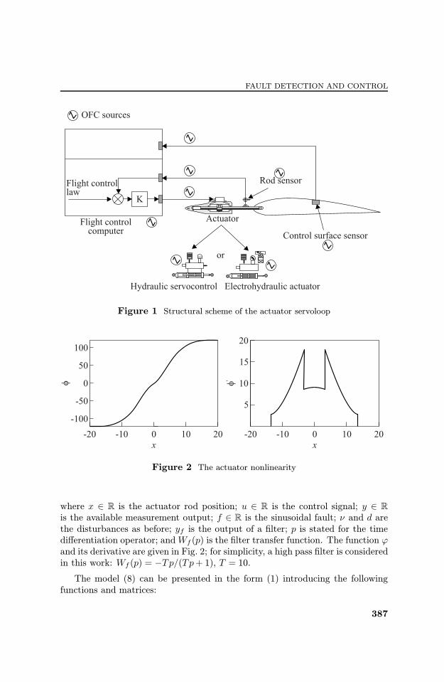
In this section, the ideas presented in this paper are illustrated through ana-lytical design of a harmonic oscillatory failure case detector in electronic §ightcontrol system [20]. These faults may result in an unwanted control surface os-cillation, generating unacceptably high loads or vibrations on the aircraft struc-ture. The capability to detect robustly and as fast as possible these failuresis very important because it has an impact on the structural design of theaircraft. In this paper, only failures located in the servocontrol loop of themoving surfaces is considered [20]. Habitually, such type of failure generatesspurious sinusoidal signals (mainly, due to electronic components) propagat-ing through the servocontrol loop, leading to control surface oscillation (seeFig. 1, where the structural scheme of servoloop is shown). The faulty com-ponents may be located inside the §ight control computer, the analogue in-puts/outputs, the position sensors, or the actuators. The §ight control com-puter may also generate unwanted oscillations of the command current sentto the actuator servovalve. The fault signals are considered to be sinusoidalwith amplitude and frequency uniformly distributed over the range 1 10 Hz(above 10 Hz, the failure has no signi¦cant e¨ects because of the low-pass na-ture of the actuator). The detection time is expressed in period numbers, thusdepending on the failure frequency, the time permissible for detection is vary-ing.The following actuator model is considered [20]:

‘x(t) = ϕ [yf(t)− x(t) + u(t) + f(t)] + ν(t) ;yf(t) =Wf (p) [x(t) − u(t)− f(t)] ;y(t) = x(t) + d(t)

⎫⎪⎪⎬

⎪⎪⎭

(8)

386

FAULT DETECTION AND CONTROL

Figure 1 Structural scheme of the actuator servoloop

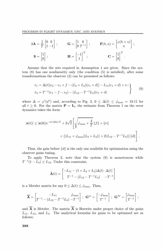
Figure 2 The actuator nonlinearity

where x ∈ R is the actuator rod position; u ∈ R is the control signal; y ∈ R

is the available measurement output; f ∈ R is the sinusoidal fault; ν and d arethe disturbances as before; yf is the output of a ¦lter; p is stated for the timedi¨erentiation operator; andWf (p) is the ¦lter transfer function. The function ϕand its derivative are given in Fig. 2; for simplicity, a high pass ¦lter is consideredin this work: Wf (p) = −Tp/(Tp+ 1), T = 10.The model (8) can be presented in the form (1) introducing the following

functions and matrices:

387

PROGRESS IN FLIGHT DYNAMICS, GNC, AND AVIONICS

3A =1T

[0 01 −1

]

; G =[1 00 T−1

]

; F(h, u) =[ϕ(h+ u)

u

]

;

S =[10

]

; H =[−11

]T

; C =[10

]T

.

Assume that the sets required in Assumption 1 are given. Since the sys-tem (8) has one nonlinearity only (the condition (5) is satis¦ed), after sometransformations the observer (2) can be presented as follows:

‘e1 = –(t)[e2 − e1 + f − (L2 + L3)(e1 + d)]− L11(e1 + d) + ν ;‘e2 = T−1(e1 − f − e2)− (L12 − T−1L3)(e1 + d)

}

(9)

where – = ϕ′(ηh) and, according to Fig. 2, 0 ≤ –(t) ≤ ‘ϕmax = 18.11 forall t ≥ 0. For the matrix P = I2, the estimate from Theorem 1 on the errordynamics takes the form:

|e(t)| ≤ |e(0)|e−0.125t/T + 2√2

[√

‘ϕmax +4T‖f‖+ ‖ν‖

+(|L11 + ‘ϕmax{L2 + L3}|+ 2(L12 − T−1L3)

) ‖d‖]

.

Thus, the gain before ‖d‖ is the only one available for optimization using theobserver gains tuning.To apply Theorem 2, note that the system (9) is monotonous while

T−1(1− L3) ≥ L12. Under this constraint,

“A(t) =

[−L11 − (1 + L2 + L3)–(t) –(t)T−1 − (L12 − T−1L3) −T−1

]

is a Metzler matrix for any 0 ≤ –(t) ≤ ‘ϕmax. Then,

A =[ −L11 ‘ϕmaxT−1 − (L12 − T−1L3) −T−1

]

; Gm =[− ‘ϕmaxT−1

]

; GM =[‘ϕmaxT−1

]

;

and A is Metzler. The matrix A is Hurwitz under proper choice of the gainsL11, L12, and L3. The analytical formulas for gains to be optimized are asfollows:

388

FAULT DETECTION AND CONTROL

|A−1S| = γ(M1,M2) =

√

1 +M22

|M1 − ‘ϕmaxM2| ;

|WM (iω)| = β(ω,M1,M2) = ‘ϕmax√4 + T 2ω2

D(ω,M1,M2);

|Wm(iω)| = ‘ϕmaxTωD(ω,M1,M2)

;

D(ω,M1,M2) =√ω2(1 +M1T )2 + (M1 − Tω2 − ‘ϕmaxM2)2

where M1 = L11 and M2 = 1− L12 + L3 are new tuning parameters. Note thatmax

r∈{m,M}|W r(iω)| = |WM (iω)| = β(ω,M1,M2) .

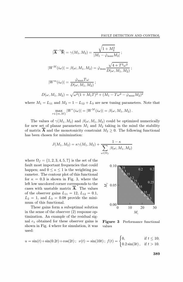
The values of γ(M1,M2) and β(ω,M1,M2) could be optimized numericallyfor new set of planar parameters M1 and M2 taking in the mind the stabilityof matrix A and the monotonicity constraint M2 ≥ 0. The following functionalhas been chosen for minimization:

J(M1,M2) = κγ(M1,M2) +1− κ

∑

ω∈Ÿf

β(ω,M1,M2)

where Ÿf = {1, 2, 3, 4, 5, 7} is the set of the

Figure 3 Performance functionalvalues

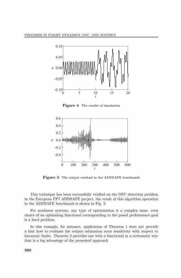
fault most important frequencies that couldhappen; and 0 ≤ κ ≤ 1 is the weighting pa-rameter. The contour plot of this functionalfor κ = 0.3 is shown in Fig. 3, where theleft low uncolored corner corresponds to thecases with unstable matrix A. The valuesof the observer gains L11 = 12, L12 = 0.1,L2 = 1, and L3 = 0.08 provide the mini-mum of this functional.These gains form a suboptimal solution

in the sense of the observer (2) response op-timization. An example of the residual sig-nal e1 obtained for these observer gains isshown in Fig. 4 where for simulation, it wasused:

u = sin(t)+sin(0.2t)+cos(2t) ; ν(t) = sin(10t) ; f(t) =

{0, if t ≤ 10;0.2 sin(3t) , if t > 10.

389

PROGRESS IN FLIGHT DYNAMICS, GNC, AND AVIONICS

Figure 4 The results of simulation

Figure 5 The output residual in the ADDSAFE benchmark

This technique has been successfully veri¦ed on the OFC detection problemin the European FP7 ADDSAFE project, the result of this algorithm operationin the ADDSAFE benchmark is shown in Fig. 5.

For nonlinear systems, any type of optimization is a complex issue, evenchoice of an optimizing functional corresponding to the posed performance goalis a hard problem.

In this example, for instance, application of Theorem 1 does not providea hint how to evaluate the output estimation error sensitivity with respect toharmonic faults. Theorem 2 provides one with a functional in a systematic waythat is a big advantage of the presented approach.

390

FAULT DETECTION AND CONTROL

7 CONCLUDING REMARKS

The problem of nonlinear observer design for fault detection with optimizedperformance is studied. It is assumed that the plant model contains unknownparameters and it is subjected by external disturbances and faults. Two ap-proaches for observer design are presented. The ¦rst one is based on solution ofLMIs, its novelty consists in introduction of additional observer gains in the con-ventional routine for LMI-based observer design. The additional observer gainsmay be used for performance optimization. The second method uses monotonic-ity assumption on the estimation error dynamics, it introduces a new tool todesign nonlinear observers. An advantage of the second approach is that it givesa simple technique to tune the observer gains in order to optimize the faultdetection performance and robustness. E©ciency of the proposed approach isdemonstrated through the oscillatory failure case in aircraft surface servoloops.

ACKNOWLEDGMENTS

The authors are grateful for the provision of an EU FP7 grant ADDSAFE (FP7-233815) which funded this work.

REFERENCES

1. Chen, J., and R. J. Patton. 1999. Robust model-based fault diagnosis for dynamicsystems. Kluwer Academic Publs.

2. Ding, S.X. 2008. Model-based fault diagnosis techniques. Design schemes, algo-rithms, and tools. Heidelberg, Berlin: Springer.

3. Borto¨, S.A., and A.F. Lynch. 1995. Synthesis of optimal nonlinear observers.34th Conference on Decision and Control Proceedings. 95 100.

4. Ding, S.X., T. Jeinsch, P.M. Frank, and E. L. Ding. 2000. A uni¦ed approach tothe optimization of fault detection systems. Int. J. Adaptive Control Signal Proc.14:725 45.

5. Wang, J., G. Yang, and J. Liu. 2007. An LMI approach to H index and mixedH /H1 fault detection observer design. Automatica 43:1656 65.

6. Casavola, A., D. Famularo, and G. Franze. 2008. Robust fault detection of uncertainlinear systems via quasi-LMIs. Automatica 44:289 95.

7. Li, X., and K. Zhou. 2009. A time domain approach to robust fault detection oflinear time-varying systems. Automatica 45:94 102.

8. Zhong, M., S.X. Ding, and E. L. Ding. 2010. Optimal fault detection for lineardiscrete time-varying systems. Automatica 46:1395 400.

391

PROGRESS IN FLIGHT DYNAMICS, GNC, AND AVIONICS

9. Leondes, C.T., and J. F. Yocum. 1975. Optimal observers for continuous time linearstochastic systems. Automatica 11(1):61 73.

10. Simon, D. 2006. Optimal state estimation: Kalman, H in¦nity, and nonlinear ap-proaches. Wiley-Interscience.

11. Poznyak, A., A. Nazin, and D. Murano. 2004. Observer matrix gain optimization forstochastic continuous time nonlinear systems. Systems Control Lett. 52(5):377 85.

12. Abbaszadeh, M., and H. J. Marquez. 2008. RobustH∞ observer design for sampled-data Lipschitz nonlinear systems with exact and Euler approximate models. Auto-matica 44(3):799 806.

13. Moisana, M., O. Bernard, and J.-L. Gouz‚e. 2009. Near optimal interval observersbundle for uncertain bioreactors. Automatica 45(1):291 95.

14. Nijmeijer, H., and T. I. Fossen. 1999. New directions in nonlinear observer design.London, U.K.: Springer-Verlag.

15. Besanƒcon, G., ed. 2007. Nonlinear observers and applications. Lecture notes incontrol and information science ser. Berlin: Springer Verlag. 363.

16. Smith, H. L. 1995. Monotone dynamical systems: An introduction to the theory ofcompetitive and cooperative systems. Surveys and monographs. Providence: AMS.41.

17. Lee, L.H. 1997. Identi¦cation and robust control of linear parameter-varying sys-tems. PhD Thesis. Berkeley, CA: University of California at Berkeley.

18. Bokor, J., and G. Balas. 2004, Detection ¦lter design for LPV systems ¡ ageometricapproach. Automatica 40:511 18.

19. Ra�Šssi, T., G. Videau, and A. Zolghadri. 2010. Interval observers design for consis-tency checks of nonlinear continuous-time systems. Automatica 46(3):518 27.

20. Goupil, P. 2010. Oscillatory failure case detection in the A380 electrical §ight con-trol system by analytical redundancy. Control Eng. Practice 18:1110 19.

21. Arcak, M., and P. Kokotovi‚c. 2001. Nonlinear observers: A circle criterion designand robustness analysis. Automatica 37:1923 30.

22. Alcorta-Garcia, E., A. Zolghadri, and P. Goupil. 2011. A nonlinear observer-basedstrategy for aircraft oscillatory failure detection: A380 case study. IEEE Trans.Aerospace Electronic Syst. 47(4):2792 806.

23. Pomet, J. B., and L. Praly. 1992. Adaptive nonlinear regulation: Estimation fromthe Lyapunov equation. IEEE Trans. Automatic Control AC-37:729 40.

24. Sontag, E.D. 2007. Input to state stability: Basic concepts and results. In: Non-linear and optimal control theory. Eds. P. Nistri and G. Stefani. Berlin: Springer-Verlag. 163 220.

25. Pavlov, A.V., N. van de Wouw, and H. Nijmeijer. 2007. Frequency response func-tions for nonlinear convergent systems. IEEE Trans. Automatic Control 52:1159 65.

26. Sontag, E. D. 2002. Asymptotic amplitudes and cauchy gains: A small-gain prin-ciple and an application to inhibitory biological feedback. Systems Control Lett.47:167 79.

392