A Risk Evaluation Approach for Pit Slope Design · Cases of rock slope with stable and failed...

1. INTRODUCTION The methodology described in this paper is the result of the work carried out by the authors during the past five years for various mining projects, confronted always with similar needs of providing management with appropriate information to base decisions on the pit slope configurations to be developed. The use of traditional methods of slope design does not always fulfill these requirements resulting either in uneconomical or high risk designs.

The two traditional methods of slope design, namely those based on the calculation of factor of safety and

probability of failure are examined and their main drawbacks are highlighted to introduce the risk analysis methodology for slope design presented in this paper.

The use of the methodology is then illustrated with the description of three study cases where it has been successfully applied. The projects correspond to the feasibility evaluation of the Cerrejon Coal Mine in Colombia, the slope steepening project at Chuquicamata mine in Chile and the slope design assessment for an unnamed (due to confidentiality requirements) open pit mine in Asia.

ARMA 08-231 A Risk Evaluation Approach for Pit Slope Design Steffen, O. K. H., Contreras, L. F., Terbrugge, P. J., Venter, J. SRK Consulting, Johannesburg, South Africa

Copyright 2008, ARMA, American Rock Mechanics Association This paper was prepared for presentation at San Francisco 2008, the 42nd US Rock Mechanics Symposium and 2nd U.S.-Canada Rock Mechanics Symposium, held in San Francisco, June 29-July 2, 2008. This paper was selected for presentation by an ARMA Technical Program Committee following review of information contained in an abstract submitted earlier by the author(s). Contents of the paper, as presented, have not been reviewed by ARMA and are subject to correction by the author(s). The material, as presented, does not necessarily reflect any position of ARMA, its officers, or members. Electronic reproduction, distribution, or storage of any part of this paper for commercial purposes without the written consent of ARMA is prohibited. Permission to reproduce in print is restricted to an abstract of not more than 300 words; illustrations may not be copied. The abstract must contain conspicuous acknowledgement of where and by whom the paper was presented.

ABSTRACT: The determination of the acceptable slope angle for open pits is a key aspect of the mineral business, as it implies seeking the optimum balance between the additional economic benefits gained from having steeper slopes, and the additional risks resulting from the consequent reduced stability of the pit slopes. The difficulty in determining the acceptable slope angle is related to geological uncertainties within the rock mass. These uncertainties are accounted for in the process of slope design and different methodologies have been used for this purpose. The traditional approach is that based on the calculation of the factor of safety (FOS), where the uncertainties are accounted for through the selection of a FOS for design larger than 1.0. A methodology more frequently used in recent years is that based on the calculation of the probability of failure (POF) of the slope, where input parameters to the deterministic model of the previous approach are represented by probability distributions to assess the probability of having a FOS less than a critical value representing the failure of the slope. Although in the POF approach uncertainties are partially accounted for, a major drawback that still persists in both the FOS and POF methodologies is the difficulty to define an adequate acceptability criterion. A methodology that aims to solve this problem is the risk analysis approach. In slope design, risk can be defined as the POF of the slope combined with the consequence or potential loss associated with the failure of the slope. The consequences can be two fold: personnel impact and economic impact. The proposed methodology of risk evaluation considers the use of non formal sources of information (engineering judgment, expert knowledge) together with hard data for the assessment of both components of the risk equation. Methods such as fault and event tree analysis are used for this purpose. The approach includes four main tasks: (1) Evaluation of the total probability of failure (POF) representative of the stability conditions of slopes. (2) Evaluation of the consequences of slope failure on safety of personnel. (3) Evaluation of the consequences of slope failure in terms of economic losses associated with impact on equipment and production. (4) Evaluation of options for risk mitigation for those cases where acceptable risk levels are exceeded. This paper describes the risk analysis methodology for slope design and presents some examples of actual projects where the methodology has been successfully applied.

2. FACTOR OF SAFETY, PROBABILITY OF FAILURE AND RISK ANALYSIS

2.1. Uncertainties in Slope Design The optimum design of a pit requires the determination of the most economic pit limit which normally results in steep slope angles as in this way the excavation of waste is minimized. In general, as the slope angle becomes steeper, the stripping ratio (waste to ore ratio) is reduced and the mining economics improves. However, these benefits are counteracted by an increased risk to the operation. Thus the determination of the acceptable slope angle is a key aspect of the mining business.

The difficulty in determining the acceptable slope angle stems from the existence of uncertainties associated with the stability of the slopes. Table 1 summarizes the main sources of uncertainty in pit slopes. These uncertainties are accounted for during the process of design of the slopes and different methodologies have been used for this purpose.

The uncertainty might be due to a random variability of the aspect under analysis or to lack of knowledge of that aspect. Field data collection and site investigations are used to reduce these uncertainties and to define the inherent natural variability. Table 1. Sources of Uncertainty in Pit Slopes

Slope Aspect Source of Uncertainty

Geometry Topography

Geology / Structures Groundwater surface

Properties Strength

Deformation Hydraulic conductivity

Loading In situ stresses

Blasting Earthquakes

Failure Prediction Model reliability

Steffen (1997) [1] has proposed a categorization of pit slope angles based on the confidence of slope design, which in turn depends on the degree of certainty which applies to the data available. The categories define proven, probable and possible slope angles according to a decreasing level of certainty in the design.

2.2. Factor of Safety Approach The oldest approach for slope design is that based on the calculation of the factor of safety (FOS). The FOS can be defined as the ratio between the resisting forces (strength) and the driving forces (loading) along a potential failure surface. If the FOS has a value of one, the slope is said to be in a limit equilibrium condition, whereas values larger than one correspond to stable slopes. The FOS approach is a deterministic technique

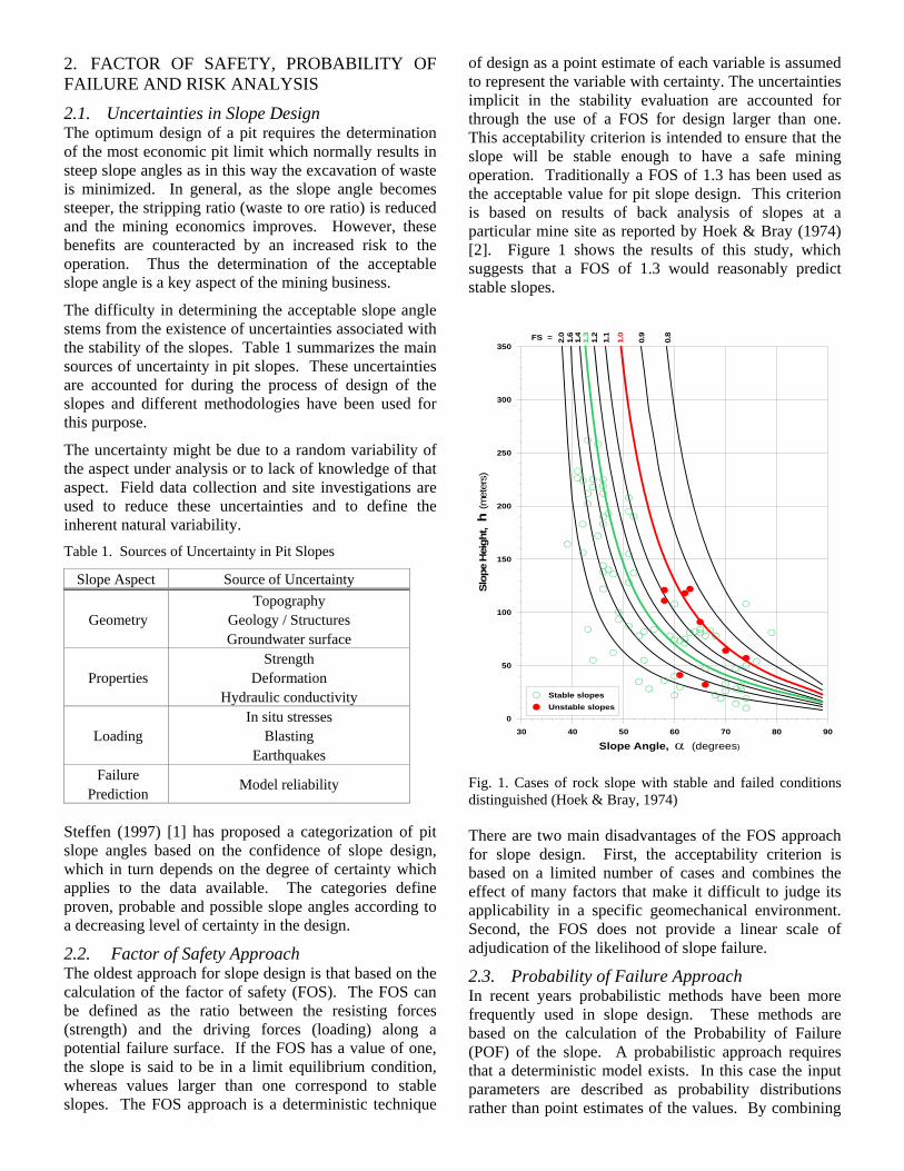
of design as a point estimate of each variable is assumed to represent the variable with certainty. The uncertainties implicit in the stability evaluation are accounted for through the use of a FOS for design larger than one. This acceptability criterion is intended to ensure that the slope will be stable enough to have a safe mining operation. Traditionally a FOS of 1.3 has been used as the acceptable value for pit slope design. This criterion is based on results of back analysis of slopes at a particular mine site as reported by Hoek & Bray (1974) [2]. Figure 1 shows the results of this study, which suggests that a FOS of 1.3 would reasonably predict stable slopes.

Fig. 1. Cases of rock slope with stable and failed conditions distinguished (Hoek & Bray, 1974)

There are two main disadvantages of the FOS approach for slope design. First, the acceptability criterion is based on a limited number of cases and combines the effect of many factors that make it difficult to judge its applicability in a specific geomechanical environment. Second, the FOS does not provide a linear scale of adjudication of the likelihood of slope failure.

2.3. Probability of Failure Approach In recent years probabilistic methods have been more frequently used in slope design. These methods are based on the calculation of the Probability of Failure (POF) of the slope. A probabilistic approach requires that a deterministic model exists. In this case the input parameters are described as probability distributions rather than point estimates of the values. By combining

30 40 50 60 70 80 90

Slope Angle, α (degrees)

0

50

100

150

200

250

300

350

Slop

e H

eigh

t, h

(m

eter

s)

2.0

1.0

0.9

0.8

1.1

1.2

1.3

1.4

1.6FS =

Stable slopesUnstable slopes

these distributions within the deterministic model used to calculate the FOS, the probability of failure of the slope can be estimated. A technique commonly used to combine the distributions is the Monte Carlo simulation. In this case each input parameter value is sampled randomly from its distribution and for each set of random input values a FOS is calculated. By repeating this process many times, a distribution of the FOS is obtained. The POF can be calculated as the ratio between the number of cases that failed (FOS<1) and the total number of simulations. The POF concept is illustrated on Figure 2.

Fig. 2 Definition of POF and Relationship with FOS according to uncertainty magnitude

The advantage of the POF over the FOS as a stability indicator is illustrated on Figure 2. By definition, there is a linear relationship between the POF value and the likelihood of failure, whereas the same is not true for the FOS. A larger FOS does not necessarily represent a safer slope, as the magnitude of the implicit uncertainties is not captured by the FOS value. A slope with a FOS of 3 is not twice as stable as one with a FOS of 1.5, whereas a slope with a POF of 5% is twice as stable as one with a POF of 10%.

Some drawbacks of the FOS methodology that persist in the POF approach are the difficulties to define an adequate acceptability criterion for design and the limitations to predict failure with the underlying deterministic model.

Acceptable criteria for POF have been defined by some researchers as indicated in Table 2 (extracted from Sjoberg (1999) [3]) and should be considered as a reference. As pointed out by Sjoberg, the actual criteria to be used in a specific mine cannot be determined from general guidelines like these, and should be subject to a more thorough analysis of the consequences of failure.

Table 2. Acceptable POF Criteria for Rock Slopes

Category and Consequence of

Failure Example POF (FOS<1)

%

Not Serious Non critical benches 10 Moderately

Serious Semi permanent slopes 1 – 2

Very Serious High/permanent slopes 0.3

Note: After Priest & Brown, 1983; Pine, 1992 2.4. Risk Analysis Approach The risk analysis approach tries to solve the main drawback of the previous methodologies with regard to the selection of the appropriate acceptability criteria. Risk can be defined as the probability of occurrence of an event combined with the consequence or potential loss associated with that event:

Risk = P(event) × Consequence of the event (1)

In the case of slopes, the P(event) is the POF of the slope and the consequences can be two fold: personnel impact and economic impact.

The POF calculated as part of the design process is normally based on a slope stability model calculation and accounts only for part of the uncertainties of the slope. Because the risk analysis sets the acceptability criteria on the consequences rather than on the likelihood of the event, a thorough evaluation of the POF of the slope is required, incorporating other sources of uncertainty not accounted for with the slope stability model. For this purpose and for the analysis of consequences of slope failure, non formal sources of information (engineering judgment, expert knowledge) are incorporated into the process with the aid of methods such as development of logic diagrams and event tree analysis. These techniques are described in detail by Harr (1996) [4], Vick (2002) [5] and Baecher and Christian (2003) [6].

In the following sections, a description of the specific approach followed for a mine study is presented.

3. APPROACH OF RISK ANALYSIS There are many methods available for developing a risk consequence process. However, they all contain some common steps, as described in the guidelines by the Australian Geomechanics Society (2000) [7]. These are:

(i) Identify the event generating hazards; (ii) Assess the likelihood or probability of occurrence

of these events; (iii) Assess the impact of the hazard; (iv) Combine the probability and impact to produce an

assessment of risk;

FOS = 1.0Limit equilibrium

FOS = 1.35Low uncertainty

FOS = 1.50High uncertainty

POF correspondsto relative area beneath

curve to the leftof FOS = 1.0 line

FOS < 1.0Unstable slope

FOS > 1.0Stable slope

1.00 FOSA FOSB

FOSA < FOSB however POFA = POFB

FREQ

UEN

CY

FOS

POFB

POFA

FOS = 1.0Limit equilibrium

FOS = 1.35Low uncertainty

FOS = 1.50High uncertainty

POF correspondsto relative area beneath

curve to the leftof FOS = 1.0 line

FOS < 1.0Unstable slope

FOS > 1.0Stable slope

1.00 FOSA FOSB

FOSA < FOSB however POFA = POFB

FREQ

UEN

CY

FOS

POFBPOFB

POFAPOFA

(v) Compare the calculated risk with benchmark criteria to produce an assessment of risk, and

(vi) Use the assessment of risk as an aid to decision making.

The work described in this paper refers mainly to steps (ii) to (v) of this methodology applied to the risk assessment of pit slopes.

The risks associated with a major slope failure can be categorized by the following consequences:

• Injury to personnel. • Damage to equipment. • Economic impact on production. • Force Majeure (a major economic impact). • Industrial action. • Public relations, such as stakeholder resistance,

environmental impact, etc.

Three of the six consequences are all economically related, although on different scales. These differentiated scales equate to the acceptable risk (or the risk criterion) that would apply to each case. Commercial risks quantified must be acceptable to the mine owners, and are related to the probability of failure

of the slopes evaluated through the risk assessment methodology. Safety risks are usually regarded as outside management discretion with most companies seeking compliance with industry norms or other indicators of societal tolerance.

The diagram presented in Figure 3 illustrates the methodology used for the risk consequence analysis of pit slopes. The scope defined for this paper includes only the first four consequences.

In particular the study consisted of the following tasks:

• Assessment of the total probability of failure (POF) representative of the stability conditions of the slopes.

• Assessment of the consequences of slope failure on safety of personnel and in terms of economic losses associated with impact on equipment and production.

• Assessment of mitigation options to reduce risk and comply with acceptability criteria.

In the following sections these tasks will be described in detail.

Fig. 3 Methodology for Risk Evaluation of Pit Slopes

PROBABILITIES OF SLOPE FAILURE CONSEQUENCES RISKS

SLOPE FAILUREUncertainties in:- Rock mass strength- Conditions of major structures- Geology- Water conditions

Effect of Model Bias

Effect of Seismic Events

Design POF

ΔPOFMOD

ΔPOFEQ

SLOPE FAILURE

Total POF

P (Fatality)

P (Economic Loss)

PERSONNEL

EQUIPMENT

PUBLIC REL.

HUMAN RES.

CONTRACTS

PRODUCTION

P (Force Majeure)

Stakeholder Resistance

Industrial Action

PROBABILITIES OF SLOPE FAILURE CONSEQUENCES RISKSPROBABILITIES OF SLOPE FAILURE CONSEQUENCES RISKS




Design POF

ΔPOFMOD

ΔPOFEQ

SLOPE FAILURE

Total POF

P (Fatality)

P (Economic Loss)

PERSONNEL

EQUIPMENT

PUBLIC REL.

HUMAN RES.

CONTRACTS

PRODUCTION

P (Force Majeure)


Industrial Action




Design POF

ΔPOFMOD

ΔPOFEQ

SLOPE FAILURE

Total POF




Design POF

ΔPOFMOD

ΔPOFEQ







Design POF

ΔPOFMOD

ΔPOFEQ

Design POF

ΔPOFMOD

ΔPOFEQ

SLOPE FAILURE

Total POF

SLOPE FAILURE

Total POF

P (Fatality)

P (Economic Loss)

PERSONNEL

EQUIPMENT

PUBLIC REL.

HUMAN RES.

CONTRACTS

PRODUCTION

P (Force Majeure)


Industrial Action

P (Fatality)P (Fatality)

P (Economic Loss)

P (Economic Loss)

PERSONNEL

EQUIPMENT

PUBLIC REL.

HUMAN RES.

CONTRACTS

PRODUCTION

P (Force Majeure)P (Force Majeure)

Stakeholder ResistanceStakeholder Resistance

Industrial Action

Industrial Action

4. PROBABILITY OF SLOPE FAILURE The objective of this task is the assessment of the likelihood of occurrence of slope failure events that might impact on personnel, equipment and production. This is done through the estimation of the probability of failure representative of the stability conditions of the slopes.

Possible slope failures are typically considered at three levels:

(i) Global, in which the entire pit wall might collapse jeopardizing the mine.

(ii) Inter-ramp, in which a partial wall failure might substantially affect the recovery of ore.

(iii) Bench, in which slope failure only affects the local operations in the vicinity of the failed bench.

In order to account for different failure modes at each of these scales, several different analysis techniques are used to calculate failure probabilities as described in specialized literature [4, 6]. However, two specific methodologies applied to the risk analysis of two of the projects described in this paper are described in the following sections, as they correspond to adaptations of general techniques to the geotechnical situations of those projects.

4.1. Source Response Diagram (SRD) Analysis It is customary to calculate the probability of failure of the slopes using a Monte Carlo technique built in to a stability analysis program to simulate the variability of uncertain factors, typically the strength parameters. This is referred to here as the design POF of the slope. However, a risk analysis involves the analysis of consequences and the probability of failure should consider all the possible uncertain factors that might lead to the failure of the slope, referred as the total POF of the slope. The total POF of slopes can be estimated through the use of Source Response Diagrams (SRD), which enable the incorporation of other sources of uncertainty not accounted for in the design of the slopes, like changes in geometry, variability of rock conditions due to geological or operational factors, changes in groundwater conditions and occurrence of seismic events. These factors represent abnormal deviations from the normal conditions assumed for the design of the slopes. Figure 4 shows a typical SRD, corresponding to the case of deviation in water conditions of a pit slope. In the diagram, the branches corresponding to other factors are indicated but not included. Chapman and Ward (2003) [8] provide an example of the source-response diagram discussed above, and describe associated leading edge project risk management processes used in a wide range of industries.

The assumed conditions representing the departure from normal conditions are evaluated with the slope stability model to calculate the effect of these situations on the POF of the slope. For this purpose, slope stability analyses are carried out with the same stability program used to evaluate the normal conditions case. Both favorable and unfavorable variations of the aspect under analysis are considered, and for each case, the possible responses during operation are evaluated in terms of their probability of occurrence. Therefore, the diagram enabled the consideration of both threats to and opportunities for the stability condition of the slope. In this way, the net contributions to the total POF resulting from the assumed variations for each aspect can be evaluated.

The SRD methodology is appropriate for those situations where there is not abundant hard data on those aspects having an influence on the stability of the slopes, although some knowledge exists on the effect of these aspects based on broad experience or on observed performance of the operation or on any other source of non formal information. It is clear that in these situations the uncertainty is large, but at least it can be incorporated into the analysis.

4.2. Monte Carlo Analysis with Response Surface Methodology

Ideally, the factor of safety distribution would be computed by the Monte Carlo method, which allows direct representation for the various uncertainties that are to be represented. In this technique, many simulations (“realizations”) are made using randomly chosen properties from the parent distributions for the various uncertainties (“assumptions”) represented in the analysis, with the results added to give a probability distribution of the computed factor of safety. Typically, several thousand realizations will be made to determine (“forecast”) the probability of performance modeled. Realistically, the Monte Carlo approach cannot be used directly with models based on numerical analyses, as each simulation in these codes takes a relatively long time. Instead, an approximate approach, often referred to as the response surface method, is available, which fits curves to numerical model results. These curves are then used in the Monte Carlo analysis. Using the response surface method, the distribution of the factor of safety for a slope can be estimated using a few runs per slope of the numerical model.

This methodology is described in detail by Morgan and Henrion (1990) [9], and a brief description follows.

If the response surface method includes say six uncertainties (denoted as x1- x6) contributing to the distribution of FOS, then this distribution could be viewed as being represented by a function

Fig. 4 Example of a SRD for deviation of water conditions of a pit slope

FOS = R(x1, x2 .. x6) (2)

In six-dimensional space, defined by variables x1- x6, R can be viewed as a surface. The response surface method assumes that the effects of each variable xi on FOS are independent of the other variables. Inaccuracies arise because this assumption is not true in general. However, these inaccuracies are minimized by calculating the best-estimate of FOS first using the best-estimates for each of the uncertainties x′1, x′2,..x′6:

FOSbe = R(x′1, x′2… x′6) (3)

where FOSbe is the best-estimate value and is referred to as the base case. Next, the change in FOS caused by change in each of the uncertainties is investigated in turn and while keeping the remaining five at their best-estimate values. An effect factor β is defined for each of the uncertainties where:

β(x1- x′1) = R(x1, x′2… x′6) / FOSbe (4)

and similarly for the other uncertainties by cyclic rotation of the indices. One point on either side of the best-estimate value (referred to as the “+” and “-”cases) is used to determine the β trends and is fitted with a 2nd order polynomial function, as illustrated on Figure 5.

Multiple Monte Carlo simulations, using the various representations of the uncertainties (typically triangular), then allow estimation of the distribution in the factor of safety using:

FOS = FOSbe . β(x1- x′1) . β(x2- x′2) . . β(x6- x′6) (5)

Some examples of the type of uncertain variables in slope stability problems that can be accounted for with this technique include:

• Characteristic GSI values. • Characteristic UCS values. • Orientation of major structures. • Shear strength of major structures. • Groundwater pressures. • Boundaries of geologic units.

The graphs in Figure 5 correspond to a situation where these six types of uncertainties have been evaluated with this technique. The curves represent the response of the FOS of the slope under analysis to variations of each of the uncertain variables. The shaded triangles represent the probability distributions used for the Monte Carlo analysis to define the distribution of FOS values for that slope.

WETTERSLOPE

POF = 12%

DRYERSLOPE

POF = 1%

SLOPE DESIGNIS ADJUSTED

AND / OR DRAINAGEIS INCREASED

FAILURETO ACHIEVE

DESIGN CONDITION


NOTHING ISDONE

NO STABILITYEFFECT

REDUCEDSTABILITY

ΔPOF = 0%

p = 5%

p = 50% p = 50% p = 5%

p = 50%

ΔPOF = +7% ΔPOF = -4%

p = 95%

ΔPOF = 0%

Net ΔPOF = + 1.56%

DEVIATIONIN WATER

CONDITIONS

NO STABILITYEFFECT

INCREASEDSTABILITY

TOTAL POF SLOPE

POF = 7.3%

Net ΔPOF = ( 0.50*0.50*7%) - (0.05*0.95*4%)

BASE CASE SLOPE

POF = 5%

DEVIATIONIN

GEOMETRY

DEVIATIONIN

GEOLOGY

DEVIATIONDUE TO

BLASTING

Net ΔPOF +0.2%

Net ΔPOF +0.3%

Net ΔPOF +0.2%

WETTERSLOPE

POF = 12%

DRYERSLOPE

POF = 1%


AND / OR DRAINAGEIS INCREASED

FAILURETO ACHIEVE

DESIGN CONDITION


NOTHING ISDONE

NO STABILITYEFFECT

NO STABILITYEFFECT

REDUCEDSTABILITYREDUCEDSTABILITY

ΔPOF = 0%

p = 5%

p = 50% p = 50% p = 5%

p = 50%

ΔPOF = +7% ΔPOF = -4%

p = 95%

ΔPOF = 0%

Net ΔPOF = + 1.56%

DEVIATIONIN WATER

CONDITIONS

NO STABILITYEFFECT

NO STABILITYEFFECT

INCREASEDSTABILITY

INCREASEDSTABILITY

TOTAL POF SLOPE

POF = 7.3%

Net ΔPOF = ( 0.50*0.50*7%) - (0.05*0.95*4%)

BASE CASE SLOPE

POF = 5%

DEVIATIONIN

GEOMETRY

DEVIATIONIN

GEOLOGY

DEVIATIONDUE TO

BLASTING

Net ΔPOF +0.2%

Net ΔPOF +0.3%

Net ΔPOF +0.2%

Fig. 5 Illustration of derived influence coefficients β for response surface

4.3. Model Uncertainty Model uncertainty arises through systematic biases in input parameter determinations and idealizations in the calculation vehicle, leading to the effect that failure occurs for some critical factor of safety that may not be unity. Bias in parameter determination is inevitable, and is handled by calibration to slope performance. Model idealizations arise for instance from representing a 3D situation with a 2D model, representing the rock mass strength with an elastic-plastic model and so forth. Some aspects of model idealization will tend to reduce FScrit (defined as the FOS corresponding to the failure condition of the slope) while other aspects might raise FScrit. The effect of the parameter bias and model uncertainty is to produce an uncertainty band that is centered on the underlying bias.

Traditionally model uncertainty has been accounted for in the choice of acceptable factors of safety. Acceptability criteria have been based on the approach of comparing slope angle with slope height from actual successful and failed slopes. This approach was used in the study of Hoek and Bray (1974) [2] that produced the results indicated in Figure 1, and more recently, in a

similar investigation by Sjoberg (2001) [3] with the introduction of a measurement of the rock strength.

The three main difficulties of this approach are: (1) it does not recognize bias in the characterization of data from one slope to another, (2) structures and scale related features that might affect each slope are not represented and (3) different failure modes are not recognized. However, all the studies confirm the existence of model uncertainty and suggest that there is a range for FScrit.

An alterative to looking at FScrit directly is to look at the actuarial failure rates versus nominal factor of safety. A risk evaluation study carried out by Golder Associates in 1997 for a highway widening in Hong Kong and described by Pine and Roberts (2005) [10], enabled the estimation of failure probability from the actual proportion of failures. Results of this study are shown on Figure 6 as the trend of FOS versus POF. The Hong Kong trend is probably biased as the engineers involved in the work noted that conservative strength estimates were used. Nevertheless, the trend line indicates 100% confidence in failure at a nominal FScrit = 0.8. Hoek and Bray’s data on Figure 1 can be converted to a similar

GSI - Influence on FS Base Case

0.800.85

0.90

0.95

1.00

1.05

1.10

1.151.20

0 0.2 0.4 0.6 0.8 1

Normalized GSI

βUCS - Influence on FS Base Case

0.80

0.85

0.900.95

1.00

1.05

1.101.15

1.20

0 0.2 0.4 0.6 0.8 1Normalized UCS

β

Dip Major Structures - Influence on FS Base Case

0.80

0.85

0.90

0.95

1.00

1.05

1.10

0 0.2 0.4 0.6 0.8 1Normalized Dip MS

β

Strength Major Structures - Influence on FS Base Case

0.80

0.850.90

0.95

1.001.05

1.10

1.151.20

0 0.2 0.4 0.6 0.8 1

Normalized Strength MS

β

Groundwater Pressure – Influence on FS Base Case

0.80

0.85

0.90

0.95

1.00

1.05

1.10

0 0.2 0.4 0.6 0.8 1

Normalized Groundwater Factor

β

Geological Boundary – Influence on FS Base Case

0.80

0.85

0.90

0.95

1.00

1.05

1.10

0 0.2 0.4 0.6 0.8 1Normalized Geological Factor

β

FOSi = FOSbase_case . β1i . β2i . β3i . β4i . β5i . β6i


0.800.85

0.90

0.95

1.00

1.05

1.10

1.151.20

0 0.2 0.4 0.6 0.8 1

Normalized GSI


0.80

0.85

0.900.95

1.00

1.05

1.101.15

1.20

0 0.2 0.4 0.6 0.8 1Normalized UCS

β


0.80

0.85

0.90

0.95

1.00

1.05

1.10


β


0.80

0.850.90

0.95

1.001.05

1.10

1.151.20

0 0.2 0.4 0.6 0.8 1


β


0.80

0.85

0.90

0.95

1.00

1.05

1.10

0 0.2 0.4 0.6 0.8 1


β


0.80

0.85

0.90

0.95

1.00

1.05

1.10


β


0.800.85

0.90

0.95

1.00

1.05

1.10

1.151.20

0 0.2 0.4 0.6 0.8 1

Normalized GSI


0.80

0.85

0.900.95

1.00

1.05

1.101.15

1.20

0 0.2 0.4 0.6 0.8 1Normalized UCS

β


0.80

0.85

0.90

0.95

1.00

1.05

1.10


β


0.800.85

0.90

0.95

1.00

1.05

1.10

1.151.20

0 0.2 0.4 0.6 0.8 1

Normalized GSI


0.80

0.85

0.900.95

1.00

1.05

1.101.15

1.20

0 0.2 0.4 0.6 0.8 1Normalized UCS

β


0.80

0.85

0.90

0.95

1.00

1.05

1.10


β


0.80

0.850.90

0.95

1.001.05

1.10

1.151.20

0 0.2 0.4 0.6 0.8 1


β


0.80

0.85

0.90

0.95

1.00

1.05

1.10

0 0.2 0.4 0.6 0.8 1


β


0.80

0.85

0.90

0.95

1.00

1.05

1.10


β

FOSi = FOSbase_case . β1i . β2i . β3i . β4i . β5i . β6iFOSi = FOSbase_case . β1i . β2i . β3i . β4i . β5i . β6i

form by counting the number of failures at a given nominal FOS versus the number of cases in the database and assuming that the data shown on the figure is a representative sample. The results of this conversion are also plotted on the graphs of Figure 6 and also indicate 100% confidence in failure at a nominal FScrit = 0.8.

Fig. 6 Computed FOS versus probability of slope failure from various studies

The definition of the FScrit distribution to represent model uncertainty has two aspects; one is the selection of the best estimate value, and the other is its assumed variability.

In terms of the best estimate value of FScrit, it is considered that the departures from 1.0, which is the value normally assumed to represent failure, would be better justified by the calibration of the stability model used in a particular situation, based on results from back analysis of failures. These values can then be adjusted on the basis of engineering judgment and benchmarking of results of the FOS versus POF relationships derived from other studies as described before. Figure 7 shows an example of the results of a benchmarking analysis performed for a pit slope where an FScrit of 1.05 was assumed.

In terms of the variability of FScrit it might be estimated from engineering judgment based on the degree of confidence gained on the ability of the stability model to predict failure conditions in a particular site environment. Intensive benchmarking against the actual performance of the slopes through back analysis of failed slopes greatly contributes to increase this confidence.

Fig. 7 Benchmarking of pit slope data for best estimate values of FScrit.

5. CONSEQUENCE ANALYSIS OF SLOPE FAILURE – SAFETY IMPACT The purpose of this task is the assessment of the consequences of slope failure on safety of personnel. This is done through the estimation of the probability of fatality caused by slope failures and the comparison of the results with acceptability criteria.

5.1. Event Tree Analysis for Safety Impact Event trees are used to estimate the probability of fatality and injury caused by the occurrence of slope failures. The event tree is a diagram that connects the starting event (failure of the slope) with the ultimate consequence under evaluation (fatality or injury) through a series of intermediate events based on a cause-effect relation. The events are quantified in terms of their likelihood of occurrence, thus enabling the assessment of the end outcomes in terms of their probabilities of occurrence, following the appropriate rules to operate the AND/OR operators.

Figure 8 shows the typical event tree developed for the evaluation of safety impact of pit slope failures. The components of the tree address the following questions:

• Does visual inspection detect movement? • Is there sufficient warning from visual alert? • Is the instrumentation system operational? • Is there sufficient warning from system alert? • Do monitoring people respond correctly? • Is the evacuation procedure successful? • Are there people exposed? • Is there at least one injury? • Is there at least one fatality?

Hong Kong slopes

(Golder 97)

Rock slopes

(Hoek 74)

0%

1%

10%

100%

0.7 0.9 1.1 1.3 1.5 1.7 1.9 2.1

FOS

POF Hong Kong

slopes (Golder 97)

Rock slopes

(Hoek 74)

0%

1%

10%

100%

0.7 0.9 1.1 1.3 1.5 1.7 1.9 2.1

FOS

POF 0%

1%

10%

100%

0.7 0.9 1.1 1.3 1.5 1.7 1.9 2.1

FOS

POF

East WallWest Wall

0%

1%

10%

100%

0.7 0.9 1.1 1.3 1.5 1.7 1.9 2.1

FOS

POF

East WallWest WallEast WallWest Wall

Fig. 8 Event tree diagram for evaluation of safety and equipment impact of slope failures

Probability values (P) are assigned to the answers to these questions and are a reflection of aspects like: type of failure, expected volume of the slide, typical velocity of the failure, rate of deformation, slope angle, typical proximity of equipment and personnel to the slope and similar type of considerations.

The probability of a particular consequence in the diagram of Figure 8 is calculated as the sum of the probabilities of the various possible sequences of events leading to that consequence. For instance, fatality can be the result of 10 possible sequences of events according to the diagram of Figure 8. The probability of each sequence is calculated as the product of the probabilities of the events in that sequence. For example one possible sequence of events consists of: slope failure occurs, movement was detected with visual inspection, but there was not sufficient warning from this inspection, the instrumentation system was operational, but there was not sufficient warning from this system, there were people exposed at the location of the failure and the result was a fatal event. The probabilities P assigned to the affirmative answers of the questions define those of the negative answers as they correspond to mutually exclusive events, so the sum of their probabilities should be 1 for each event.

Due to the subjective character of the probability values (P) assigned to the event components of the logic diagram, it is important to account for the uncertainty in these judgmental probabilities. This is done by using triangular distributions defined by

upper and lower values for each entry to represent the uncertainty of the input components. Figure 9 illustrates a possible assumption of uncertainty in judgment of the P values. It corresponds to a maximum variability of 20% which is reduced linearly as the P values get closer to the limits of the range of variation. A Monte Carlo analysis of the event tree defined in this way enable the definition of distributions for each consequence calculated, thus enabling the attainment of confidence levels to these results.

Fig. 9 Assumption of uncertainty in judgment of P values in event trees

Subjectivity associated with probability estimates is a way of capturing and integrating expert judgment,

0.9 NO 0.02 NO

0.2 0.1 YES 0.5 NO 0.98 YES 0.2 NO 0.1 YES

0.5 YES 0.8 YES 0.3 NO 0.3 YES 0.9 NO 0.5 YES

0.7 YES 0.1 NO 0.7 NO 0.5 NO

0.9 YES

FATALITY / EQUIPMENT

DEMOLISHED

SUCCESSFUL EVACUATION PROCEDURE?

NO INCIDENT / NO IMPACT

3 x 10-3

1.4 x 10-2

1.8 x 10-1

INJURY / EQUIPMENT DAMAGED

AT LEAST ONE INJURY? /

EQUIPMENT IMPACTED?

AT LEAST ONE FATALITY? / EQUIPMENT

DEMOLISHED?

SLOPE FAILURE

PEOPLE / EQUIPMENT EXPOSED?

MONITORING PEOPLE

RESPOND CORRECTLY?

SUFFICIENT WARNING OF

FAILURE? (visual

inspection)

SUFFICIENT WARNING OF

FAILURE? (monitoring

system)

VISUAL INSPECTION

DETECTS MOVEMENT?

INSTRUMENTATION SYSTEM

OPERATIONAL?

P

± ΔP

0.2 0.5 0.80 1

0.2

10.82x - 1

x0 0.22x

x0 0.22x

x 0.5X- 0.2

xX + 0.2

P

± ΔP

0.2 0.5 0.80 1

0.2

P

± ΔP

0.2 0.5 0.80 1

0.2

10.82x - 1

x0 0.22x

x0 0.22x

x 0.5X- 0.2

xX + 0.2

10.82x - 1

x0 0.22x

x0 0.22x

x 0.5X- 0.2

xX + 0.2

only some of which may be based on hard data, and it is what formal modeling of uncertainty and risk is about. Analysis which must be hard data based is inherently partial and weak. Subjectivity in risk analysis is discussed by Vick (2002) [5] and by Chapman and Ward (2002) [11].

5.2. Exposure Analysis of Personnel The probability of coincidence in time and space of mine personnel with an eventual slope failure can be estimated for the scenario in which people had not been evacuated. The approach uses information on equipment fleet and personnel working during the year to assess the percentage of time in a year that workers are exposed to slope failures. Table 3 presents an example of this analysis. Table 3 Exposure Analysis for Personnel

Description No. Hours

exposed / year

Total hours /

year

% exposure /

year Drill Operator 3 22,338 26,280 85 Blasting Crew 10 61,320 87,600 70 Shovel Operator 4 28,733 35,040 82 Dozer Operator 10 70,080 87,600 80 Truck Operator 28 183,960 245,280 75 Water car Operator 2 3,504 17,520 20 FELoader Operator 2 6,132 17,520 35 Maintenance 25 21,900 219,000 10 Supervisors 5 6,570 43,800 15 Surveyors 2 1,752 17,520 10 Geologists 3 2,102 26,280 8 Geotech engineers 3 1,314 26,280 5

The exposure results presented in Table 3 represent the time in a year spent by the different workers within the pit. However, these values need to be adjusted to account for the fact that the likelihood of impact from a failure event is also determined by the location of the worker relative to the slope (i.e. closer to the toe as opposed to far from a potential slide) and by the mobility of the equipment dictated by the mining operation routines (i.e. standing close to new mined faces as opposed to old existing slopes). These exposure factors are estimated based on the geometry of the slopes, volume of the potential slides, statistical data on the actual performance of equipment and mobility of personnel and equipment during the course of normal operations.

In a particular open pit mine situation, it might be the case that shovel operators are estimated to be within the reach zone of a potential slope failure for 60% of the operation cycle. Also, that they are within the pit areas prone to be affected by slope failures for 80% of the operational time. In this case for a calculated exposure of 82% as indicated in Table 3, the adjusted

exposure would be 82%×0.6×0.8 = 39%. Typically the maximum exposure calculated is carried forward to the event tree analysis.

5.3. Probability of fatality Results of the worker safety assessment are represented by the annual probability of fatality (APF) values derived from the event tree analysis using the annual personnel exposure data. The typical representation of results is indicated in Figure 10 where the APF have been plotted versus the year for two alternative mining plans. This analysis is carried out for the most representative sections of the slope. Because the APF results correspond to distributions, values with a particular confidence can be selected for evaluation. The results plotted in Fig. 8 correspond to 50% and 90% confidence levels that they will not be exceeded. The curves show a distinct increase in risk toward the end of the life of the open-pit mine and suggest the need for mitigation strategies.

The safety evaluations are carried out for the various scale of slope failure i.e. global, inter-ramp and bench scale, as each one of those imposes different types of threats to safety of personnel.

Fig. 10 Typical results of safety evaluation for global failure on the west wall.

5.4. Acceptability Criteria for Safety Impact In order to assess the meaning of the calculated probability of fatality values, they need to be compared with benchmark criteria. A typical graph used for this purpose is indicated in Figure 11 which presents acceptability criteria for fatality defined by different sources. This type of plot is normally called an F-N diagram. The areas in the graph related with tolerability of risk are derived from risk guidelines developed in the United Kingdom [12], and

0.00001

0.0001

0.001

0.01

0.1

Ann

ual P

roba

bilit

y Fa

talit

y

P50 Plan 1P90 Plan 1P50 Plan 2P90 Plan 2

0 2 4 6 8 10 12Year

0.00001

0.0001

0.001

0.01

0.1

Ann

ual P

roba

bilit

y Fa

talit

y



0 2 4 6 8 10 12Year

0 2 4 6 8 10 120 2 4 6 8 10 12Year

correspond to risk thresholds in terms of local acceptability of deaths from industrial and other accidents. It is plotted as the number of fatalities from accidents versus the annual probability of exceeding that number.

Fig. 11 Benchmark Criteria for Safety Impact of Slope failure

The “Local Tolerability Line” defines a region which is characterized by both high frequencies and severe consequences (the “Intolerable” region). The region between this line and the “Local Scrutiny Line” is a region of possibly unjustifiable risk. Between this latter line and the “Negligibility Line” is a region which is judged to be tolerable but for which all reasonably practicable steps should be taken to reduce the hazard further. This is the ALARP region (As Low As Reasonably Practicable). All combinations of frequency and number of fatalities which fall below the “Negligibility Line” are considered to be negligible.

The graph also contains fatality criteria developed by the dam engineering discipline, which is of interest as bench mark criteria, because it is based on a conservative approach to risk, since the consequences of dam failures are so devastating. Of particular interest is the single fatality at an annual probability of 10-4 identified as “The proposed BC Hydro individual risk”. This number represents the risk exposure to ‘natural death’ by the safest population group in North America aged between 10 to 14 years within a person’s life cycle. The interpretation is that 1 in 10 000 persons between the ages of 10 and 14

years will die every year from natural causes. This is also popularly accepted as the boundary between voluntary and involuntary risk. Accepting this as a criteria for slope design, implies, therefore, that a person subjected to the open pit working environment is not exposed to greater death risk resulting from a slope failure than he is of dying due to natural causes.

6. CONSEQUENCE ANALYSIS OF SLOPE FAILURE – ECONOMIC IMPACT The objective of this task is the assessment of the consequences of slope failure in terms of economic losses caused by impact on equipment and production. This is done through the estimation of the probability of occurrence of these losses and their associated costs.

6.1. Consequence Analysis for Equipment Impact

The consequence analysis for the assessment of impact of slope failures on equipment is very similar to that described for personnel safety impact. The event tree for this analysis contain similar questions to those used for the personnel safety analysis, and the same arguments given to support the inputs are applicable, but in this case, the new values refer to impact on equipment rather than on workers. In general the values for equipment reflect the lesser mobility and more difficult successful evacuation of equipment as compared with personnel.

Impact on equipment is the first of three economic criteria from slope failures. From an economic scale perspective it is the smallest of the three and an event which is commonly encountered in the open pit mining arena, i.e. a first order cost. Typically the economic implications could imply an additional cost in the range of US$10M to US$30M in any one year. Economic impact is firstly the cost of repair or replacement of equipment and secondly the loss of production that may result. The latter is often the more important consequence.

6.2. Event Tree Analysis for Economic Impact Figure 12 shows the typical event tree developed for the evaluation of economic impact of slope failures. The components of the tree addressed the following questions:

• Is ore production affected? • Can contracts be met? • Are costs prohibitive? • Can production be replaced by spot purchase? • Are there additional costs?

10,0001,000100101

10-1

10-2

10-3

10-4

10-5

10-6

10-7

Number of Fatalities, N

Ann

ual F

requ

ency

of N

or m

ore

fata

litie

s, F

1:10

1:100

1:1,000

1:10,000

1:100,000

1:5,000

1:1’000,000

1:10’000,000

INTOLERABLE

NEGLIGIBLE

ALARP REGION

UK Health & Safety Executive

Netherlands legislation

Negligibility Line

Local Tolerability LineLocal Scrutiny Line

Possibly Unjustifiable RiskHONG KONG upper risk guidelines

BC Hydro societal

BC Hydro individual

risk

10,0001,000100101

10-1

10-2

10-3

10-4

10-5

10-6

10-7


Ann

ual F

requ

ency

of N

or m

ore

fata

litie

s, F

1:10

1:100

1:1,000

1:10,000

1:100,000

1:5,000

1:1’000,000

1:10’000,00010,0001,00010010 10,0001,000100101

10-1

10-2

10-3

10-4

10-5

10-6

10-7

1

10-1

10-2

10-3

10-4

10-5

10-6

10-7


Ann

ual F

requ

ency

of N

or m

ore

fata

litie

s, F

1:10

1:100

1:1,000

1:10,000

1:100,000

1:5,000

1:1’000,000

1:10’000,000

1:10

1:100

1:1,000

1:10,000

1:100,000

1:5,000

1:1’000,000

1:10’000,000

INTOLERABLE

NEGLIGIBLE

ALARP REGION

UK Health & Safety Executive

Netherlands legislation

Negligibility Line

Local Tolerability LineLocal Scrutiny Line

Possibly Unjustifiable RiskHONG KONG upper risk guidelines

BC Hydro societal

BC Hydro individual

risk

Fig. 12 Event tree diagram for evaluation of economic impact of slope failures

The probability values assigned to the answers to this question are the reflection of aspects such us: type of failure, expected volume of the slide, typical velocity of the failure, location of slide in relation to access ramps, availability of alternative ore sources and similar type of considerations.

The analysis enables the evaluation of the probabilities associated with each of the three possible consequences in terms of economic impact, i.e. Force Majeure event, loss of profit or minor impact represented by normal operating conditions. The calculation uses the same rules and considerations described for the case of safety impact. The results are obtained in the form of distributions so that values can be defined for a desired level of confidence.

6.3. Probability of Loss of Profit The loss of profit is the second order of costs that could be incurred due to a slope failure, and would typically range from US$50M to US$200M. It is mainly associated with slope failure at inter-ramp and global scale.

A typical representation of results is presented in Figure 13 as trends with time for each of the mining plans evaluated. Results are reported in terms of annual probability of loss of profit for confidence levels of 50% (broken lines) and 90% (solid lines). There are no fixed criteria that can be assigned to this

consequence as it is dependent on the client’s appetite for risk balanced against the benefits accrued from the additional risks.

Fig. 13 Typical results of loss of profit impact caused by slope failure of two plans compared

6.4. Probability of Force Majeure Force Majeure is the third order of economic impact evaluated and represents the event of a slope failure of such magnitude that ore production is severely affected

0.2 YES

0.7 YES 0.8 NO

0.3 YES 0.3 NO 0.8 YES

0.2 0.7 NO 0.2 NO

0.1 YES

0.99 YES 0.9 NO

0.01 NO

2.6%

NORMAL OP. COND.

LOSS OF PROFIT

OVERALL SLOPE FAILURE

ORE PRODUCTION AFFECTED?

0.1%

17.3%

FORCE MAJEURE

IS COST PROHIBITIVE? (Production no

affected)

PRODUCTION REPLACED BY

SPOT?

IS COST PROHIBITIVE?

(Production affected)

FORCE MAJEURE

FORCE MAJEURECAN

CONTRACTS BE MET?

LOSS OF PROFIT

ADDITIONAL COSTS?

NORMAL OPERATING CONDITIONSLOSS OF

PROFIT

0%

10%

20%

30%

40%

50%

Ann

ual P

rob.

Los

s of

Pro

fit


0 2 4 6 8 10 12Year

0%

10%

20%

30%

40%

50%

Ann

ual P

rob.

Los

s of

Pro

fit



0 2 4 6 8 10 12Year

0 2 4 6 8 10 120 2 4 6 8 10 12Year

or could lead to the premature closure of the open pit operations.

The possible occurrence of a Force Majeure situation is normally computed for various years and integrates the results of probability of Force Majeure calculated for all the slopes and for the global and inter-ramp scale failures, as this is an event impacting the overall pit. Figure 14 presents a plot with typical results of exposure to a FM event from any slope failure for two mine plans evaluated. In this example the results clearly demonstrate the higher risk attached to Plan 2 from that of the Plan 1 case.

Fig. 14 Typical exposure to Force Majeure for two mine plans evaluated

6.5. Cost Risk Estimation The results of probabilities of FM can be combined with the cash flow values of the plans evaluated to produce graphs indicating the cost implications of the Force Majeure events. In the case of a Force Majeure event, the cost of failure equals the total loss of future NPV from the time of failure.

The curves in Figure 15 correspond to the cumulative discounted earnings and show the “actual indicated value” (thick lines), as declared in the project report, and the “including risk value” (thin lines), which in this example is defined as the 90% confidence value. The difference between these two lines for each plan corresponds to the “at risk value”, which is defined as follows:

At risk value = Actual value - 90% conf. value (6)

The actual values in this definition are based on the assumption that there is no risk of occurrence of the Force Majeure event. Technically, the curves for the situation with risk are developed from the probability of no failure occurring multiplied by the project NPV.

Fig. 15 Cost impact of Force Majeure events

Quantifying the economic value of risk according to the definition of risk used in this report is a common practice in financial institutions and the insurance industry amongst others. However, the framework of the results is slightly different. Whereas in the financial industry situation incomes are derived from the premiums or interest rates charged based on the value assessed after including the ‘cost of risk’, in the case of a mine the issue is the expected cash return from the recovery of the ore. This is conveniently expressed as the Net Present Value (NPV) with the effect of risk being reflected in the confidence that the forecast NPV will be achieved.

From a mining perspective, the lower NPV resulting from including the risk-cost calculated as shown above is not an achievable NPV within the particular mine plan in case of a Force Majeure event, but purely a perceived cost of the risk. Hence for a higher confidence (or lower uncertainty), the risk cost increases. This information therefore does not allow the decision process of trading additional benefit for increased risk. This would require alternative mine plans.

7. ANALYSIS OF MITIGATION MEASURES Risk mitigation options should be sought initially by reducing the consequences of slope failure. In this case, the inspection of the event tree diagrams used for impact assessment of slope failures enables the identification of slope management improvements to provide the maximum cost-benefit at the required acceptance criteria. An example of this would be the improvement of monitoring systems and evacuation procedures.

If the reduction of the consequences of slope failure is not sufficient to mitigate the risks to acceptable levels, options based on reducing the POF of the slope may be

0%

5%

10%

15%

20%

25%

30%

35%

Prob

abili

ty F

orce

Maj

eure


0 2 4 6 8 10 12Year

0%

5%

10%

15%

20%

25%

30%

35%

Prob

abili

ty F

orce

Maj

eure



0 2 4 6 8 10 12Year

0 2 4 6 8 10 120 2 4 6 8 10 12Year

NPV Plan 2

NPV Plan 1

0

500

1,000

1,500

2,000

2,500

3,000

3,500

4,000

Cum

mul

ativ

e D

isco

unte

d Ea

rnin

gs, $ Actual value Plan 1

Actual value Plan 290% conf. value Plan 190% conf. value Plan 2

0

1

2

Note: Illustrative scale of $

Year1 3 4 5 8 102 6 7 9 11

NPV Plan 2

NPV Plan 1

0

500

1,000

1,500

2,000

2,500

3,000

3,500

4,000

Cum

mul

ativ

e D

isco

unte

d Ea

rnin

gs, $ Actual value Plan 1

Actual value Plan 290% conf. value Plan 190% conf. value Plan 2

Actual value Plan 1Actual value Plan 290% conf. value Plan 190% conf. value Plan 2

0

1

2

Note: Illustrative scale of $

Year1 3 4 5 8 102 6 7 9 11

Year1 3 4 5 8 102 6 7 9 111 3 4 5 8 102 6 7 9 11

required. These options include unloading and/or dewatering of slopes.

7.1. Mitigation Options for Safety Impact In terms of worker safety and equipment impact, primary options are aimed at reducing the effects of slope failure, which is done through improvement of slope management procedures. An example of this is the implementation of enhanced monitoring systems (radar systems, seismic methods, extensometers, TDR systems, etc.) to provide early warning of failures. The effect of these measures can be evaluated by adjusting the appropriate values in the event trees.

7.2. Mitigation Options for Economic Impact Mitigation options to reduce the risk of economic impact include geotechnical options aimed at reducing the probability of failure of the slopes and mine planning options that target the reduction of failure impacts by looking for alternatives to maintain the planned ore feed. Examples of these measures are the implementation of flexible ramp access systems, the use of stock pile sources and so forth.

8. EXAMPLES OF APLICATION OF RISK METHODOLOGY The methodology described before has been applied in several mine projects at different stages of development. Three of those projects have been selected to illustrate the use of the methodology in real case situations.

8.1. The Cerrejon Coal Mine Risk Evaluation

• Background. The risk study carried out at the Cerrejon coal mine [13] was aimed to assess the impacts of pit slope failure in terms of safety of personnel and destruction of equipment with economic consequences. The results of the assessment were used to identify key aspects to consider in the pit slope design process to achieve a cost effective pit design complying with the owner’s safety guidelines.

The mine is located in the northern part of Colombia, over an area of approximately 50 km long by 15 km wide as indicated on Figure 16. The planned mine was to be developed over 14 different areas, with open pits excavated along the strike of target coal seams. The final pits would consist of box cuts defined by footwall, highwall and endwall slopes, with typical final heights of 240 m.

For the purpose of the study, the pit geometry was idealized as shown on Figure 17 and the mine was assumed to be represented by 7 of these pits.

• Probability of failure of slopes. The POF of typical footwall and highwall slopes was initially calculated with a slope stability program based on a limiting equilibrium analysis and using a Monte Carlo technique to account for the variability of the strength parameters. POF values of 5% for individual benches in the footwall slopes and 0.25% for the inter-ramps in the highwall slopes were defined. These values represented the normal conditions for design and were used as the base case to estimate the total POF of the slopes using the analysis of SRD described in section 4.1.

Fig. 16 Layout of Cerrejon coal mine

Fig. 17 Idealized geometry of pit slopes

The SRD analysis enabled the incorporation of other sources of uncertainty not included in the initial analysis such as changes in the slope geometry,

50 Km

15 Km

Coal bedding

1

2

3

4

5

6 7

8

9

10

11 12

13 14

Scale - Kilometers

Cerrejon Coal Mine Pit Areas

50 Km

15 Km

Coal bedding

1

2

3

4

5

6 7

8

9

10

11 12

13 14

50 Km

50 Km

15 Km15 Km

Coal beddingCoal bedding

1

2

3

4

5

6 7

8

9

10

11 12

13 14

Scale - Kilometers


Scale - Kilometers


Scale - KilometersScale - Kilometers


Advance per year174 m

FOOTWALL SLOPE

HIGHWALL SLOPE

PRODUCTION FACE

BACKFILLSLOPE

250 m

200 m

1330 m

1800 m

A

A

60 m steps60 m steps63º

35º

20º60 m steps

38 m ramps

30 m

Footwall Slope

16º

240 m

75 m

55 m

Highwall Slope

Section A-A


FOOTWALL SLOPE

HIGHWALL SLOPE

PRODUCTION FACE

BACKFILLSLOPE

250 m

200 m

1330 m

1800 m

A

A


FOOTWALL SLOPE

HIGHWALL SLOPE

PRODUCTION FACE

BACKFILLSLOPE

250 m

200 m

1330 m

1800 m


FOOTWALL SLOPE

HIGHWALL SLOPE

PRODUCTION FACE

BACKFILLSLOPE

250 m

200 m

1330 m

1800 m

A

A

A

A


35º

20º60 m steps

38 m ramps

30 m

Footwall Slope

16º

240 m

75 m

55 m

Highwall Slope

Section A-A60 m steps60 m steps63º

35º

20º60 m steps

38 m ramps

30 m

Footwall Slope

16º

240 m

75 m

55 m

Highwall Slope


35º

63º63º

35º35º

20º20º60 m steps

38 m ramps 38 m ramps

30 m30 m

Footwall Slope

16º16º

240 m240 m

75 m

55 m

Highwall Slope

Section A-A

variability of rock conditions due to geological or operational factors, changes in groundwater conditions and occurrence of seismic events. Total POF values of 7.3% and 0.5% were defined for footwall and highwall slopes, respectively. These results indicated that the uncertainties not accounted for in design added 2.3% and 0.25% to the design POF (normal conditions) of these slopes, respectively.

• Analysis of safety impact. Event trees similar to that presented on Figure 8 were used to estimate the probability of fatality and injury caused by the occurrence of slope failures. A core part of the analysis was the evaluation of personnel exposure to slope failures, which was based on a typical pit layout (Fig. 17) consistent with the planned annual production, and the equipment fleet and personnel required for its operation. Exposure factors were then estimated for fixed equipment and for trucks, using simple relationships derived from the geometry of the idealized pit and considering statistical data on the actual performance of equipment [13]. The results of this analysis suggested low exposures for the footwall slopes, with a critical value in the order of 1% for the operators of the electric shovels; and exposures between 10% and 13% for the highwall slopes corresponding to the waste truck drivers.

The probability of fatality values calculated separately for the footwall and highwall slopes through the event tree analysis were integrated using the concept of system reliability to define probability of fatality values at pit domain and mine domain level. This probability of fatality has an annual character as a result of the exposure analysis being performed on an annual basis.

The concept of system reliability for the assessment of impacts at mine domain is illustrated in equation (7). Here p mine is the probability of the impact at mine domain, p pit is the probability of the impact at pit domain and n is the number of pits.

p mine = 1 – (1 – p pit) n (7)

The comparison of the annual probability of fatality calculated for the mine with benchmark criteria based on guidelines developed in the UK (Fig. 11) indicated a level of risk categorized as ALARP (As Low as Reasonably Practicable), which was considered to be consistent with the level of information available for design and the stage of development of the project.

The results of the assessment of safety impact indicated that the probability of fatality due to slope failure would be driven by highwall slope stability. Also, the analysis of the event trees suggested that the implementation of strategies for management of slope failures such as the enhancement of monitoring

systems at highwall slopes and the improvement of evacuation procedures would cause an effective reduction of safety impact, thus enabling the mine to comply with planned targets.

• Analysis of economic impact. The risk of economic loss due slope failures was limited to the impact on equipment, as the flexibility of the operation given by the particular characteristics of the mine suggested a very low likelihood of major impacts on production caused by a slope failure. The evaluation was performed through event tree analysis in a similar fashion to that carried out for the safety impact. The analysis included the evaluation of equipment exposure to slope failures, which was based on the same considerations and assumptions made for the analysis of personnel exposure.

The event tree analysis was used to establish the probability of an economic loss associated with total or partial loss of equipment, using the failure of the slope as the initiating event. The analysis considered typical groups of equipment (equipment modules) exposed at footwall and highwall slopes, which were assumed to be impacted by failures to estimate the value of the loss. Events of similar cost at each slope type were then combined to estimate the probability of occurrence of that loss for the overall mine.

The costs of the impacts were calculated as the sum of: the cost of replacement of the equipment, the cost of lost production and the cost of cleaning the site. The results of the analysis indicated that impacts on shovels had a greater economic consequence and a smaller probability of occurrence, than impacts on trucks. The estimated cost of impacts on shovels was in the order of US$ 25 million, whereas cost of impacts on trucks was about US$ 4 million, corresponding to economic conditions of year 2005. In general the probabilities of these impacts were very low with estimated values of less that 1%.

• Conclusions. The study served to show the advantages of using this methodology in the mine design process, in particular for the identification of the main risk sources where the acquisition of geotechnical information should be focused to reduce uncertainty. Specific recommendations to reduce the risk of safety impact from slope failure were derived from the study. Economic losses caused by impact on equipment were also evaluated and critical factors causing this impact identified. In general the study indicated that highwall stability was a key factor to be considered in the design process in order to achieve a cost effective pit slope design.

8.2. The Chuquicamata Open Pit Risk Evaluation

• Background The possibility of increasing the pit slope angles of the Chuquicamata Mine as the pit approaches its planned closure motivated the execution of a quantitative risk evaluation [14] of two alternative mine plans representing the conventional mine design and a slope steepening criterion. The latter was understood to raise the NPV of the mine, but also, attracted an increase in possible adverse outcomes related to the increase in the likelihood of slope failures. The study was undertaken to provide information to assist the mine management in their decision by: defining risks in terms of safety and economics, quantifying risk level for the two slope configurations and comparing results against industry norms.

The mine is located in the northern part of Chile, in the Chuqui Porphyry complex and the orebody occurs east of the major north/south trending crustal fault known as the “west fault”. The open-pit slope performance is distinctly different in the west and east slopes as a result of the local geology. The west slope is in constant deformation and behaves as a rock mass under plastic deformation during failure, while in contrast, the east slope behaves in a brittle mode during failure. In addition, there are differences in structure and properties on a finer scale; therefore, the pit was divided into several zones and sub-zones for the stability analysis as shown on Figure 18.

Fig. 18 Plan view showing geotechnical units and geomechanical zones.

The two geometries corresponding to the two mining options subject of the study are indicated in the east-west cross-section shown on Figure 19. This section also shows the current slope configuration at the time of the study. The steeper slope configuration (PND

plan) corresponds to a double-bench arrangement and results in an increase of 2° to 5° in the inter-ramp angle and about 5% in the overall slope height, in relation to the base case option (REF plan).

Fig. 19 Comparison of current and proposed pit slopes

• Probability of failure of slopes Six principal uncertainties were considered for the evaluation of the probability of failure: (1) rock strength deviation (represented by UCS and GSI variability), (2) structural feature deviation (variability of dip and strength of major faults), (3) geological deviation (variability of boundaries of geological units), (4) groundwater pressure deviation, (5) seismic loading and (6) model reliability (variability of FScrit).

The process involved two steps: (1) calculation of the FOS distribution based on the uncertainties of the slope and (2) estimation of model bias as a distribution in FScrit. The combination of these two distributions provided a distribution in the probability of slope failure under normal conditions. Then the effect of earthquake loading was added to define the distribution of probability of failure that was carried forward into the assessment of consequences for each slope.

The calculation of the FOS distribution was based on a Monte Carlo analysis using the Response Surface methodology described in section 4.2. The FOS values required for this analysis were calculated with the programs UDEC and FLAC from ITASCA for the global and inter-ramp slopes, respectively. For inter-ramp and bench scale slopes structurally controlled failures modes were also analyzed with wedge stability models. The estimation of the FScrit distribution was done with the procedure described in section 4.3.

• Analysis of safety impact The event tree shown in Figure 8 was used to estimate the probability of fatality caused by slope failures. Input values to the diagram were defined for the various scenarios of analysis considered. Personnel exposure values were calculated based on records of performance of equipment and assumptions on personnel mobility within the pit.

N

NN

The main results of the safety impact analysis for the final pit configuration were plotted in FN diagrams of the type illustrated on Figure 11 for representative cases from the PND and REF plans. Results for both plans fell within the ALARP region, with a higher risk for the PND plan as expected. In general the analysis indicated that bench scale failures were the more relevant events in terms of safety impact and that effective mitigation of this consequence could be achieved with measures like improvement of systems for failure detection and warning.

• Analysis of economic impact The economic impact of failures was evaluated at three different scales: (1) impact on equipment, (2) impact on production with a loss of profit consequence and (3) a Force Majeure event corresponding to the biggest economic consequence.

The impact on equipment was based on a fault tree analysis similar to that performed for the safety impact. The results showed that equipment loss potential was the less critical of the slope failure consequences evaluated as the maximum calculated impact was well below the reference acceptability criterion of 10% used for all the slope scales analyzed.

The impact on production was evaluated with a fault tree analysis using the diagram shown in Figure 12. Probabilities of loss of profit and Force Majeure events were calculated for the global and inter-ramp scale failures, for different years of the pit life and for the two plans analyzed. The results were collected in graphs that showed the increase in the risk levels as the pit becomes deeper. Results were compared with reference acceptable values of 10% for loss of profit and 2% for Force Majeure, although, these criteria have a commercial character and they should be the prerogative of the mining executives.

The results of Force Majeure impact were also combined with the cash flow values of the two plans as described in section 6.5 to assess the cost of risk associated with this type of events.

• Conclusions. The risk evaluation process followed to compare the two alternative mine plans provided the mine management with a more thorough base of information on which to base decisions. The analysis enabled the identification of those slope scenarios (scale of failure, slope location, mine plan and year of mine life) having a major impact on the safety and economic consequences of slope failure, and enabled the formulation of more effective mitigation measures to reduce risks and optimize the mine plan.

8.3. Risk Evaluation for an Unnamed Open Pit Mine in Asia

• Background. A review of the geotechnical risk was carried out at a large open pit mine that was experiencing instability issues at the time. Both the operating stacks and inter-ramp slopes showed signs of instability. The design with risk process was applied to the mine design resulting in an upgrade in the slope monitoring and evacuation procedures, as well as a re-assessment of the design of the ramp access which was subsequently altered to provide greater flexibility in high risk areas.

• Safety of Personnel and Equipment. A situation existed where a shovel operation was being carried out at the base of a 60 m high slope that was considered to have a high risk of instability as illustrated in Figure 20. With personnel being exposed to failure at the base of the slope, the risks were quantified and it was found that with the existing slope monitoring and evacuation procedures in place, the risk of a fatality was found to be 3.1 × 10-3. This is above the accepted threshold, but with an enhanced monitoring system, including robotic equipment and a Ground ProbeTM radar system, together with an enhanced evacuation procedure, the risk of a fatality was reduced to 6 × 10-5, which is well below the threshold of 10-4.

Fig. 20 Potential slope failure considered for the risk analysis.

A similar exercise carried out for equipment damage or loss indicated a higher risk due to the fact that equipment cannot be moved out of the hazard area timeously. In this case consideration to damage or loss of equipment would need to be considered.

Extent ofFailure

Run Out

Extent of Failure

N

Extent ofFailure

Run Out

Extent of Failure

Extent ofFailure

Run Out

Extent of Failure

Extent ofFailure

Run Out

Extent of Failure

NNN

• Economic Consequences of Slope Failure. In carrying out the stability assessment in the south eastern sector of the pit where deterioration of the single access ramp slope had taken place, it was found that the mine would have a 15 % chance of being exposed to a US$ 3 million incident. While this amount may have been acceptable to the mine, re-establishment of access to the ore was a major consideration with the push back costs not included in the evaluation.

• Conclusion. In utilizing the system, risk to personnel and equipment, together with the economic consequences of failure could be quantified in terms of the probability of failure and loss of profits to the organization, both criteria of which are well understood by the mine management teams or executives responsible for operations. The methodology applied to this mine situation highlighted the importance that mine management takes proactive decisions on acceptable risk criteria which is independent of any technical input, so that mine designs can be developed by the technical staff to achieve the corporate objectives of acceptable risk versus reward.

9. CONCLUSIONS The risk analysis methodology presented has shown how the system can be applied to evaluate the consequences of failure in terms of personnel safety and economic impact. Also, the method has been useful in the definition of risk mitigation options pertaining to mine design procedures.

The system provides the opportunity to quantify the risks and mitigation measures for a design approach based on accepting slope failures, and as such, it can be an extremely powerful tool in the mine design process. It also provides the opportunity to rationalize the geotechnical information requirements, once the risk criteria have been defined by management.

The evaluation of risk in terms of NPV at risk is a useful approach in comparing the performance of alternative mine plans. However, for the purpose of committing to a particular mine plan, the estimated likelihoods of particular consequences of all slope failures need to be adjudicated and assessed against an acceptable risk to the mining operation. This ultimately requires judgment using all the knowledge available as well as having a full understanding of all uncertainties.

REFERENCES 1. Steffen, O.K.H. 1997. Planning of open pit mines on

a risk basis. Journal of SAIMM, March / April 1997.

2. Hoek, E. and J.W. Bray. 1974. Rock slope engineering. Institution of Mining and Metallurgy, London.

3. Sjoberg, J. 1999. Analysis of large scale rock slopes. Doctoral Thesis, Lulea University of Technology, Division of Rock Mechanics, Lulea, Sweden.

4. Harr, M.E. 1996. Reliability-based design in civil engineering. Dover Publications, Inc., Mineola, New York.

5. Vick, S.G. 2002. Degrees of belief: subjective probability and engineering judgment. ASCE, Reston, Va.

6. Baecher, G.B., and J.T. Christian. 2003. Reliability and statistics in geotechnical engineering. Wiley, Chichester, U.K.

7. Australian Geomechanics Society. 2000. Landslide risk management concepts and guidelines. AGS Sub-Committee on Landslide Risk Management, Sydney, Australia, March 2000.

8. Chapman, C. and S. Ward. 2003. Project Risk Management: Processes, Techniques and Insights. Second Edition, Wiley, 148-150.

9. Morgan, M.G. and M. Henrion. 1990. Uncertainty: a guide to dealing with uncertainty in quantitative risk and policy analysis. Cambridge University Press.

10. Pine, R.J. and W.J. Roberds. 2005. A risk-based approach for the design of rock slopes subject to multiple failure modes – illustrated by a case study in Hong Kong. International Journal of Rock Mechanics and Mining Sciences 42 (2005), Elsevier Ltd., pp. 261 – 275.

11. Chapman, C. and S. Ward. 2002. Managing Project Risk and Uncertainty: A Constructively Simple Approach to Decision Making. Wiley.

12. Health and Safety Executive. 2001. Reducing risks, protecting people – HSE’s decision-making process. HSE books. U.K.

13. Contreras, L.F., R. LeSueur and J. Maran. 2006. A Case Study of Risk Evaluation at Cerejon Mine. In Proceedings of the International Symposium on Stability of Rock Slopes in Open Pit Mining and Civil Engineering Situations, 3-6 April 2006, Cape Town, South Africa. SAIMM. Symposium Series S44, Johannesburg, South Africa.

14. Tapia, A., L.F. Contreras, O. Steffen. 2007. Risk Evaluation of Slope Failure at the Chuquicamata Mine. In Slope Stability 2007, Proceedings of the 2007 International Symposium on Rock Slope Stability in Open Pit Mining and Civil Engineering, 12-14 September 2007, Perth, Australia. Ed. Yves Potvin, Australian Centre for Geomechanics, Perth, Australia.

A Risk Evaluation Approach for Pit Slope Design · Cases of rock slope with stable and failed...

Documents

Transcript of A Risk Evaluation Approach for Pit Slope Design · Cases of rock slope with stable and failed...