

Languages
Pages
Legal


www.monash.edu.au
1prepared from lecture material © 2004 Goodrich & Tamassia
COMMONWEALTH OF AUSTRALIA
Copyright Regulations 1969
WARNING
This material has been reproduced and communicated to you by or on behalf of Monash University pursuant to Part VB of the
Copyright Act 1968 (the Act). The material in this communication may be subject to copyright under the Act.
Any further reproduction or communication of this material by you may be the subject of copyright protection under the Act.
Do not remove this notice.

www.monash.edu.au
FIT2004
Algorithms & Data Structures L9: Balanced Trees
Prepared by: Bernd Meyer from lecture materials © 2004 Goodrich & Tamassia February 2007
www.monash.edu.au
3prepared from lecture material © 2004 Goodrich & Tamassia
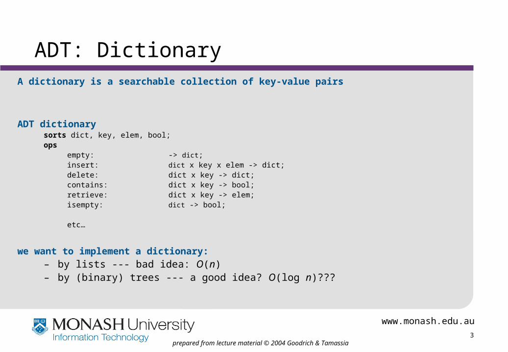
ADT: DictionaryA dictionary is a searchable collection of key-value pairs
ADT dictionarysorts dict, key, elem, bool;ops
empty: -> dict;insert: dict x key x elem -> dict;delete: dict x key -> dict;contains: dict x key -> bool;retrieve: dict x key -> elem;isempty: dict -> bool;
etc…
we want to implement a dictionary:– by lists --- bad idea: O(n)– by (binary) trees --- a good idea? O(log n)???
www.monash.edu.au
4prepared from lecture material © 2004 Goodrich & Tamassia
Search Tables
• A search table is a dictionary implemented by means of a sorted sequence– We store the items of the dictionary in an array-based sequence, sorted by key
• Performance:– find takes O(log n) time, using binary search– insert takes O(n) time since in the worst case we have to shift O(n) items to make room
for the new item– remove take O(n) time since in the worst case we have to shift O(n) items to compact
the items after the removal
• The lookup table is effective only for dictionaries of small size or for dictionaries on which searches are the most common operations, while insertions and removals are rarely performed (e.g., credit card authorizations)
www.monash.edu.au
5prepared from lecture material © 2004 Goodrich & Tamassia
Binary Search (Revision)
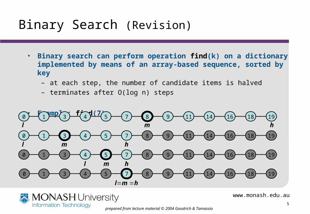
• Binary search can perform operation find(k) on a dictionary implemented by means of an array-based sequence, sorted by key– at each step, the number of candidate items is halved
– terminates after O(log n) steps
• Example: find(7)
1 3 4 5 7 8 9 11 14 16 18 19
1 3 4 5 7 8 9 11 14 16 18 19
1 3 4 5 7 8 9 11 14 16 18 19
1 3 4 5 7 8 9 11 14 16 18 19
0
0
0
0
ml h
ml h
ml h
lm h
www.monash.edu.au
6prepared from lecture material © 2004 Goodrich & Tamassia
Binary Search Trees
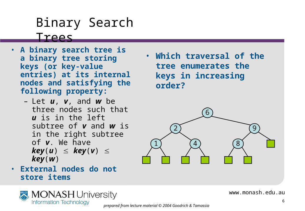
• A binary search tree is a binary tree storing keys (or key-value entries) at its internal nodes and satisfying the following property:– Let u, v, and w be three
nodes such that u is in the left subtree of v and w is in the right subtree of v. We have key(u) key(v) key(w)
• External nodes do not store items
• Which traversal of the tree enumerates the keys in increasing order?
6
92
41 8
www.monash.edu.au
8prepared from lecture material © 2004 Goodrich & Tamassia
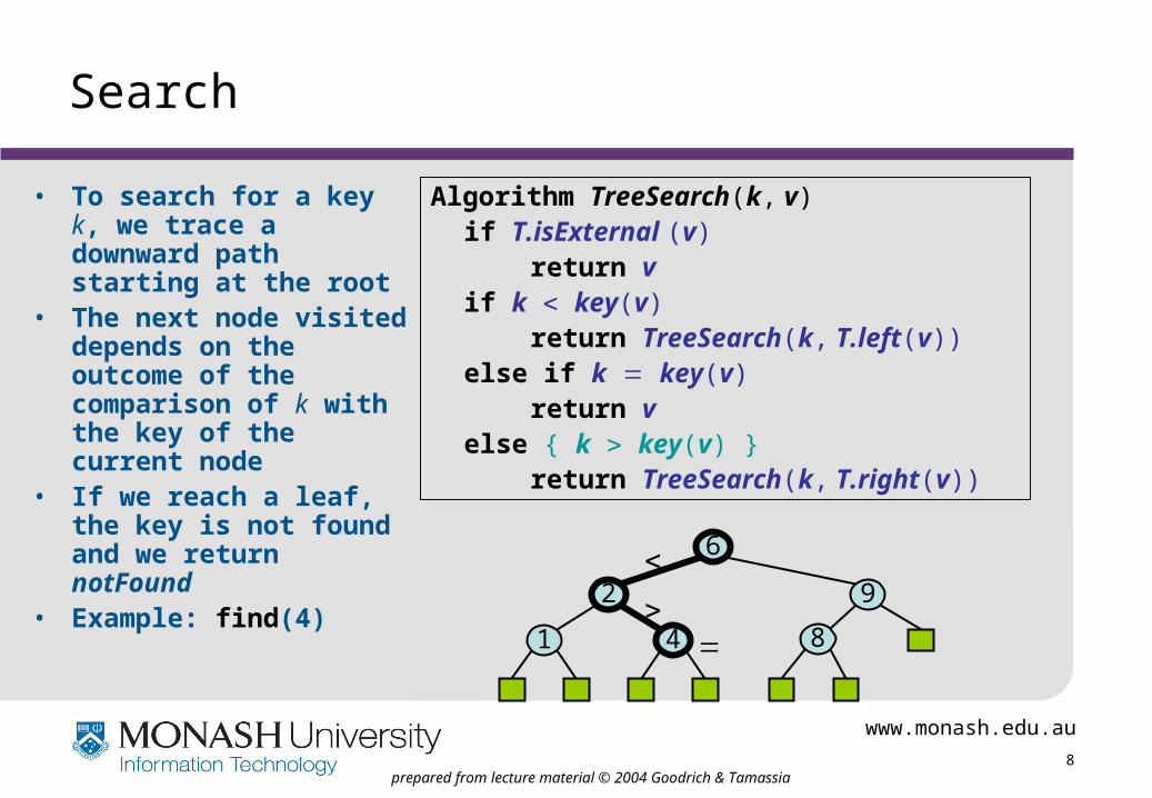
Search
• To search for a key k, we trace a downward path starting at the root
• The next node visited depends on the outcome of the comparison of k with the key of the current node
• If we reach a leaf, the key is not found and we return notFound
• Example: find(4)
Algorithm TreeSearch(k, v)if T.isExternal (v)
return vif k key(v)
return TreeSearch(k, T.left(v))else if k key(v)
return velse { k key(v) }
return TreeSearch(k, T.right(v))
6
92
41 8

www.monash.edu.au
9prepared from lecture material © 2004 Goodrich & Tamassia
Insertion
• To perform operation insert(k, o), we search for key k (using TreeSearch)
• Assume k is not already in the tree, and let let w be the leaf reached by the search
• We insert k at node w and expand w into an internal node
• Example: insert 5
6
92
41 8
6
92
41 8
5
w
w

www.monash.edu.au
10prepared from lecture material © 2004 Goodrich & Tamassia
Deletion
• To perform operation remove(k), we search for key k
• Assume key k is in the tree, and let let v be the node storing k
• If node v has a leaf child w, we remove v and w from the tree with operation removeExternal(w), which removes w and its parent
• Example: remove 4
6
92
41 8
5
vw
6
92
51 8
www.monash.edu.au
11prepared from lecture material © 2004 Goodrich & Tamassia
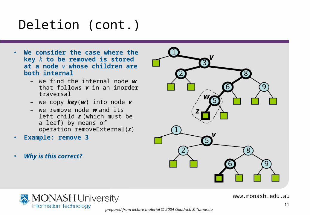
Deletion (cont.)
• We consider the case where the key k to be removed is stored at a node v whose children are both internal
– we find the internal node w that follows v in an inorder traversal
– we copy key(w) into node v– we remove node w and its left child z
(which must be a leaf) by means of operation removeExternal(z)
• Example: remove 3
• Why is this correct?
3
1
8
6 9
5
v
w
z
2
5
1
8
6 9
v
2
www.monash.edu.au
12prepared from lecture material © 2004 Goodrich & Tamassia
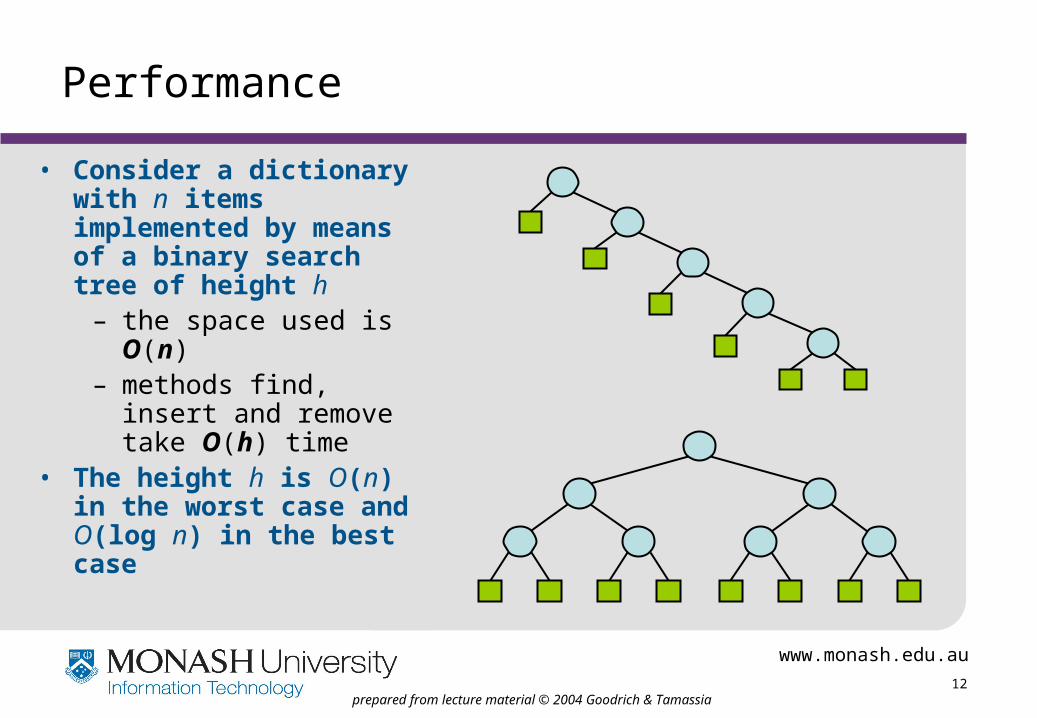
Performance
• Consider a dictionary with n items implemented by means of a binary search tree of height h
– the space used is O(n)– methods find, insert and
remove take O(h) time• The height h is O(n) in the
worst case and O(log n) in the best case
www.monash.edu.au
13prepared from lecture material © 2004 Goodrich & Tamassia
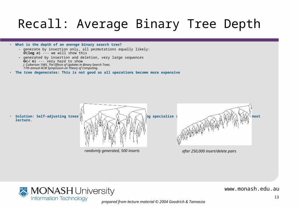
Recall: Average Binary Tree Depth
• What is the depth of an average binary search tree?– generate by insertion only, all permutations equally likely:
O(log n) --- we will show this– generated by insertion and deletion, very large sequences
( n) --- very hard to show J. Culberson 1985. The Effects of Updates in Binary Search Trees. 17th annual ACM Symposium on Theory of Computing.
• The tree degenerates: This is not good as all operations become more expensive
• Solution: Self-adjusting trees that maintain their balance using specialize (more expensive) update operations: next lecture.
randomly generated, 500 inserts after 250,000 insert/delete pairs

www.monash.edu.au
14prepared from lecture material © 2004 Goodrich & Tamassia
Dynamic Self-balancing Trees
• We cannot fully rebalance a binary tree after every operation. This is too costly.
• Thus, we cannot keep a binary tree perfectly balanced at all times.
• As an alternative we will try to relax the requirement in three different ways and hope that we still reach O(log n) access times. We will try to keep it
– almost balanced at all times (AVL Trees)– almost balanced most of the time (Splay Trees)– perfectly balanced at all times but allow it to be it non-binary (2-4-Tree, …)
www.monash.edu.au
15prepared from lecture material © 2004 Goodrich & Tamassia
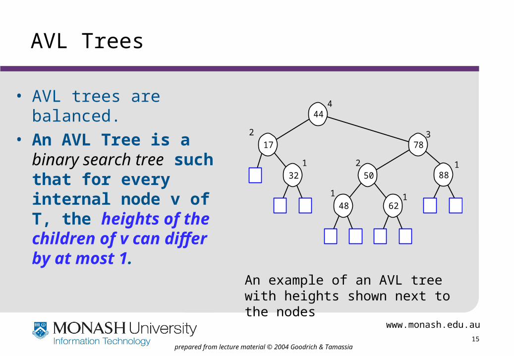
AVL Trees
• AVL trees are balanced.• An AVL Tree is a binary
search tree such that for every internal node v of T, the heights of the children of v can differ by at most 1.
88
44
17 78
32 50
48 62
2
4
1
1
2
3
1
1
An example of an AVL tree with heights shown next to the nodes
www.monash.edu.au
16prepared from lecture material © 2004 Goodrich & Tamassia
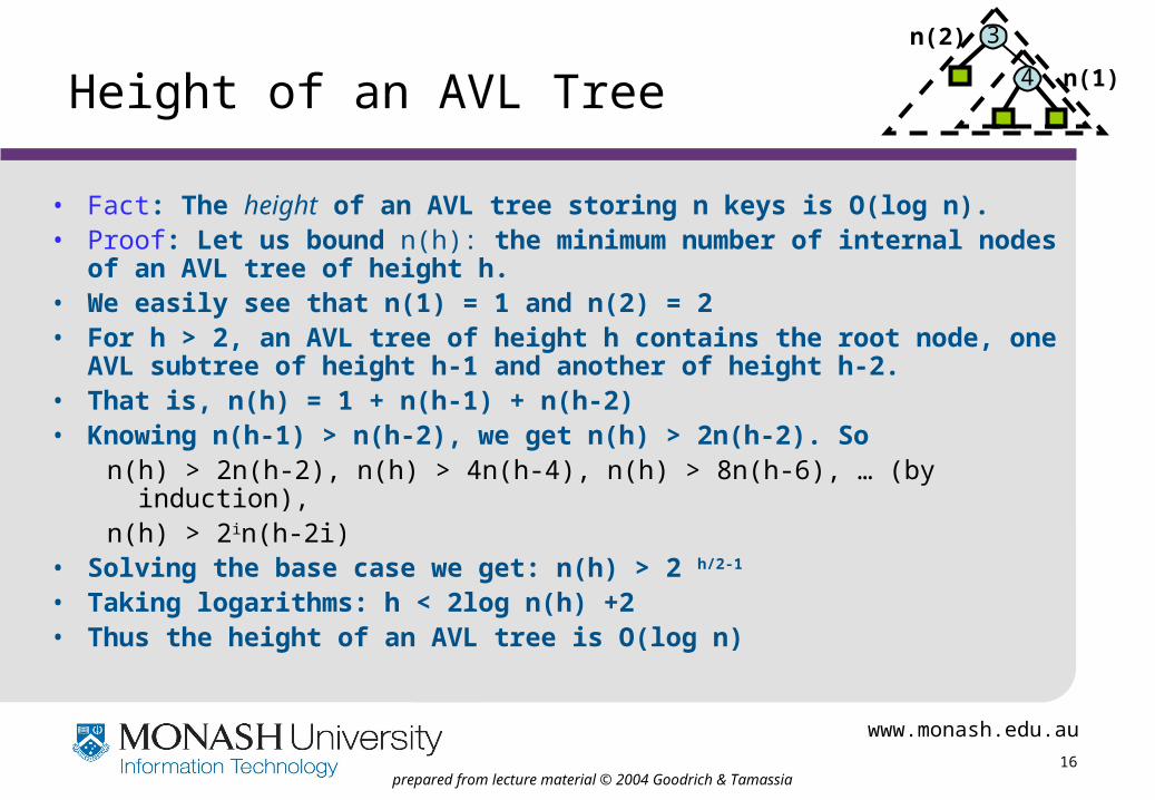
Height of an AVL Tree
• Fact: The height of an AVL tree storing n keys is O(log n).• Proof: Let us bound n(h): the minimum number of internal nodes of an
AVL tree of height h.• We easily see that n(1) = 1 and n(2) = 2• For h > 2, an AVL tree of height h contains the root node, one AVL
subtree of height h-1 and another of height h-2.• That is, n(h) = 1 + n(h-1) + n(h-2)• Knowing n(h-1) > n(h-2), we get n(h) > 2n(h-2). So
n(h) > 2n(h-2), n(h) > 4n(h-4), n(h) > 8n(h-6), … (by induction),n(h) > 2in(h-2i)
• Solving the base case we get: n(h) > 2 h/2-1
• Taking logarithms: h < 2log n(h) +2• Thus the height of an AVL tree is O(log n)
3
4 n(1)
n(2)
www.monash.edu.au
17prepared from lecture material © 2004 Goodrich & Tamassia
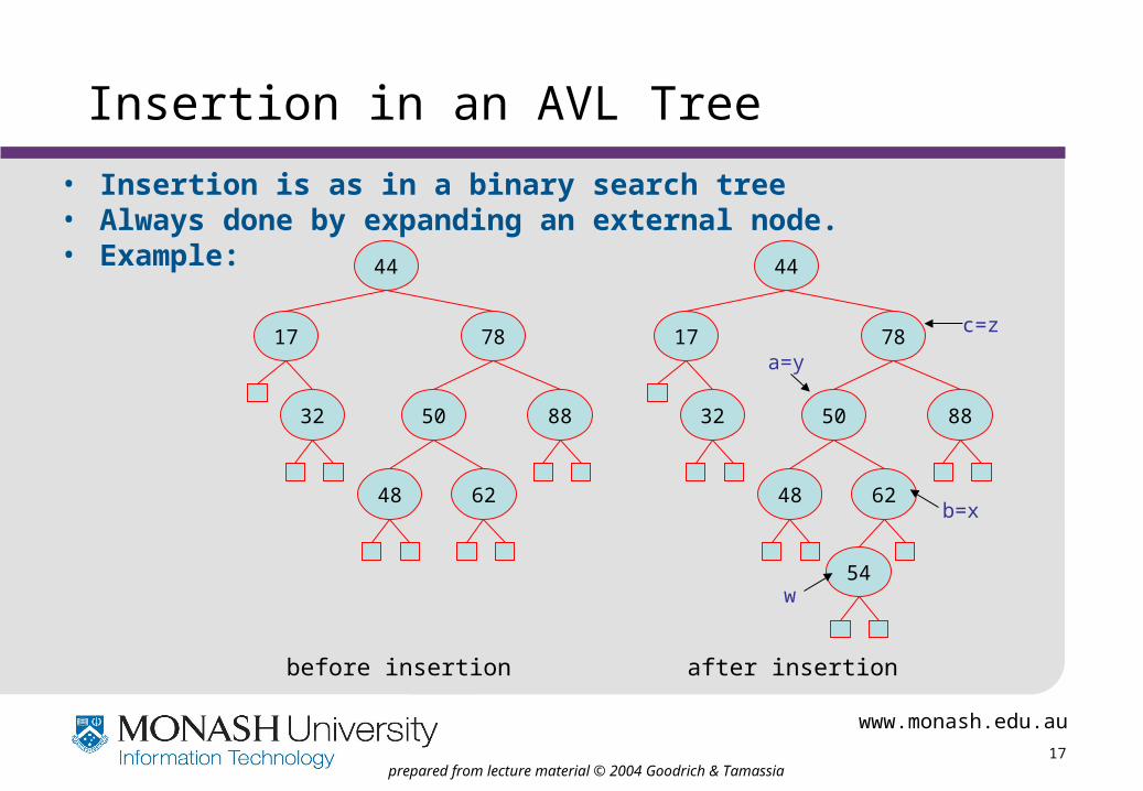
Insertion in an AVL Tree
• Insertion is as in a binary search tree• Always done by expanding an external node.• Example: 44
17 78
32 50 88
48 62
54w
b=x
a=y
c=z
44
17 78
32 50 88
48 62
before insertion after insertion
www.monash.edu.au
18prepared from lecture material © 2004 Goodrich & Tamassia
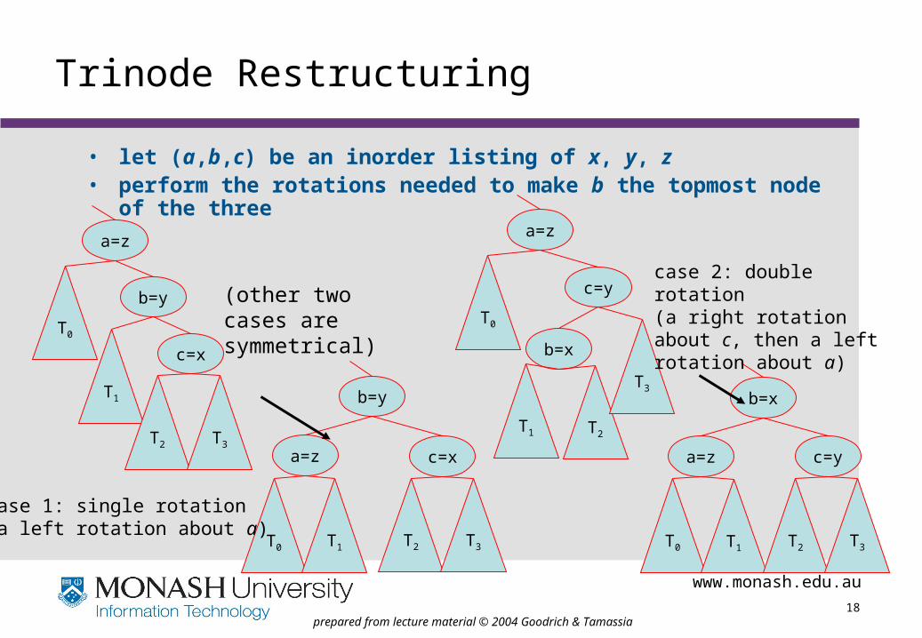
Trinode Restructuring
• let (a,b,c) be an inorder listing of x, y, z• perform the rotations needed to make b the topmost node of the three
b=y
a=z
c=x
T0
T1
T2 T3
b=y
a=z c=x
T0 T1 T2 T3
c=y
b=x
a=z
T0
T1 T2
T3b=x
c=ya=z
T0 T1 T2 T3
case 1: single rotation(a left rotation about a)
case 2: double rotation(a right rotation about c, then a left rotation about a)
(other two cases are symmetrical)
www.monash.edu.au
19prepared from lecture material © 2004 Goodrich & Tamassia
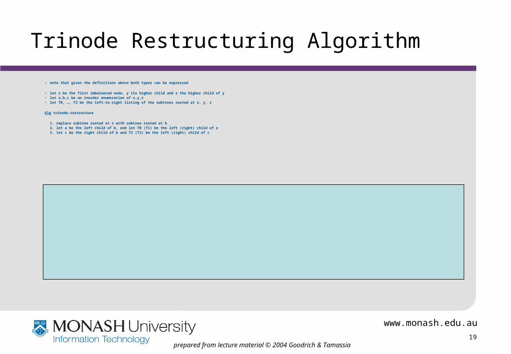
Trinode Restructuring Algorithm
• note that given the definitions above both types can be expressed
• let z be the first imbalanced node, y its higher child and x the higher child of y• let a,b,c be an inorder enumeration of x,y,z• let T0, …, T3 be the left-to-right listing of the subtrees rooted at x, y, z
Alg trinode-restructure
1. replace subtree rooted at z with subtree rooted at b2. let a be the left child of b, and let T0 (T1) be the left (right) child of a3. let c be the right child of b and T2 (T3) be the left (right) child of c
www.monash.edu.au
20prepared from lecture material © 2004 Goodrich & Tamassia
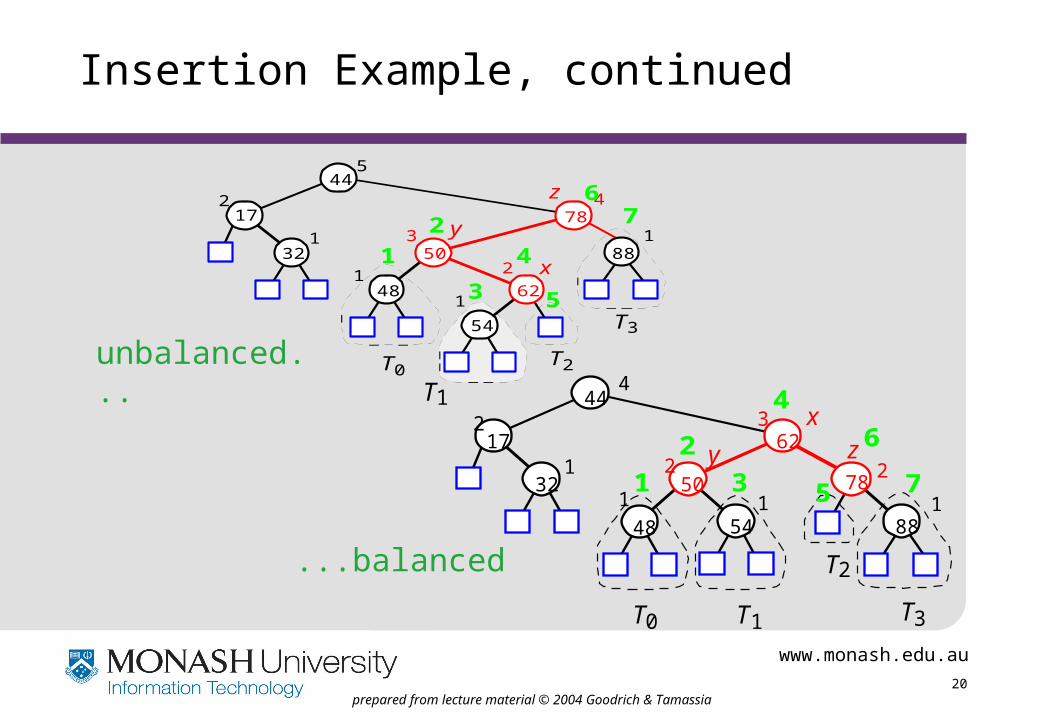
Insertion Example, continued
T0 T1 T3
unbalanced...
...balanced
88
44
17 78
32 50
48 62
2
5
1
1
3
4
2
1
54
1
T0T2
T3
x
y
z
2
3
4
5
67
1
88
44
17
7832 50
48
622
4
1
1
2 2
3
154
1
T2
x
y z1
2
3
4
5
6
7
T1

www.monash.edu.au
21prepared from lecture material © 2004 Goodrich & Tamassia
Restructuring (as Single Rotations)
• Single Rotations:
T0
T1
T2
T3
c = x
b = y
a = z
T0 T1 T2
T3
c = x
b = y
a = zsingle rotation
T3
T2
T1
T0
a = x
b = y
c = z
T0T1T2
T3
a = x
b = y
c = zsingle rotation
T0T1 T2 T3
www.monash.edu.au
22prepared from lecture material © 2004 Goodrich & Tamassia
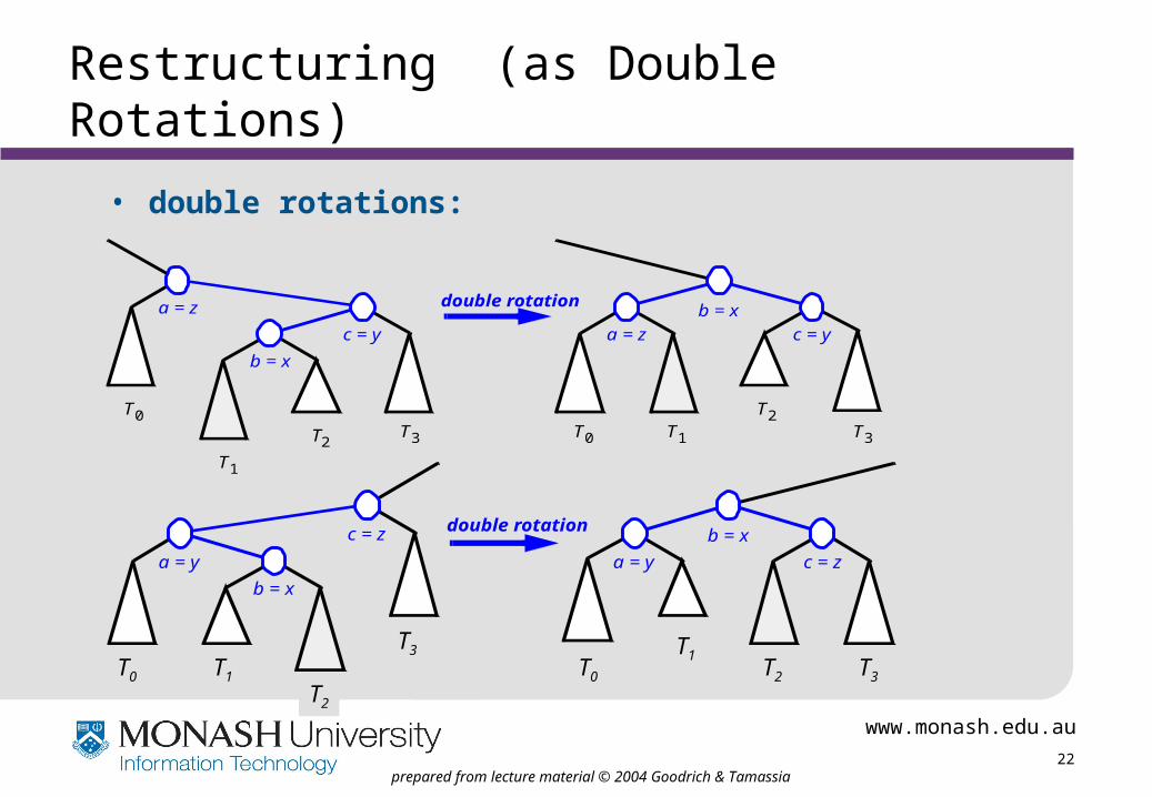
Restructuring (as Double Rotations)
• double rotations:
double rotationa = z
b = x
c = y
T0
T2
T1
T3 T0
T2T3T1
a = z
b = x
c = y
double rotationc = z
b = x
a = y
T0
T2
T1
T3 T0
T2T3 T1
c = z
b = x
a = y
T0
T1T2 T3T0 T1
T2
T3
www.monash.edu.au
23prepared from lecture material © 2004 Goodrich & Tamassia
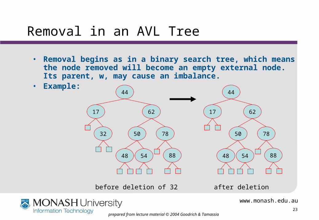
Removal in an AVL Tree
• Removal begins as in a binary search tree, which means the node removed will become an empty external node. Its parent, w, may cause an imbalance.
• Example: 44
17
7832 50
8848
62
54
44
17
7850
8848
62
54
before deletion of 32 after deletion
www.monash.edu.au
24prepared from lecture material © 2004 Goodrich & Tamassia
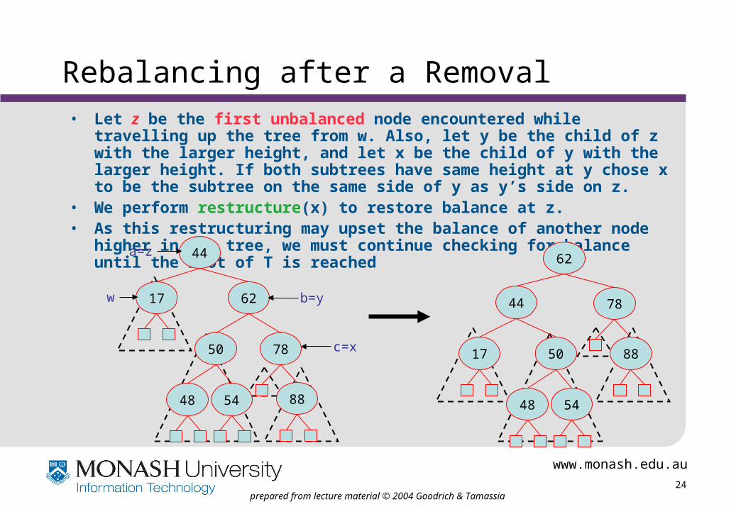
Rebalancing after a Removal• Let z be the first unbalanced node encountered while travelling up the tree
from w. Also, let y be the child of z with the larger height, and let x be the child of y with the larger height. If both subtrees have same height at y chose x to be the subtree on the same side of y as y’s side on z.
• We perform restructure(x) to restore balance at z.• As this restructuring may upset the balance of another node higher in the
tree, we must continue checking for balance until the root of T is reached44
17
7850
8848
62
54
w
c=x
b=y
a=z
44
17
78
50 88
48
62
54
www.monash.edu.au
25prepared from lecture material © 2004 Goodrich & Tamassia
Running Times for AVL Trees
• a single restructure is O(1)– using a linked-structure binary tree
• find is O(log n)– height of tree is O(log n), no restructures needed
• insert is O(log n)– initial find is O(log n)– Restructuring at the node, restoring heights
• remove is O(log n)– initial find is O(log n)– Restructuring up the tree, maintaining heights is O(log n)
www.monash.edu.au
26prepared from lecture material © 2004 Goodrich & Tamassia
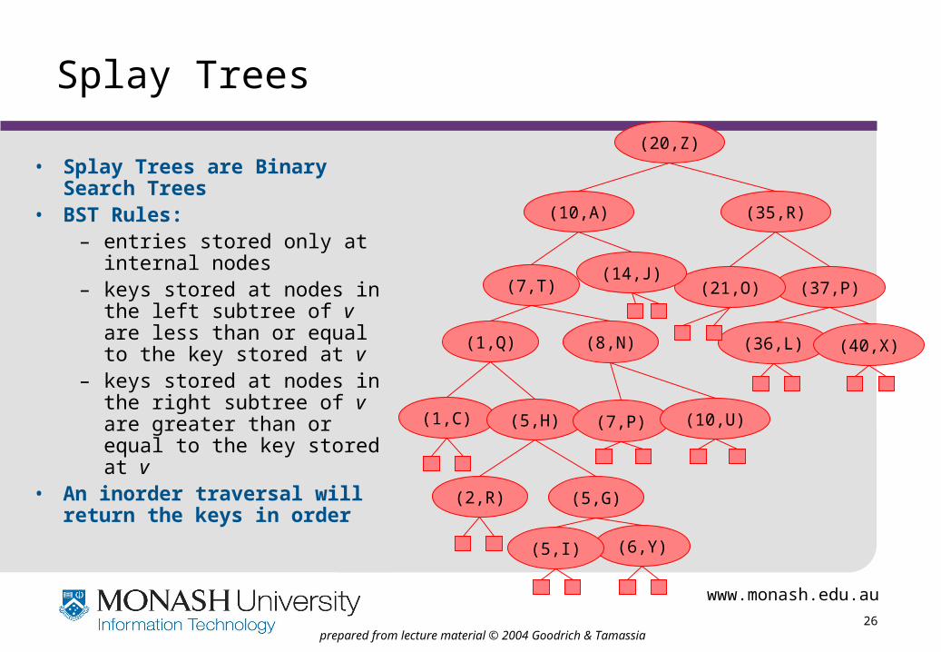
Splay Trees
• Splay Trees are Binary Search Trees
• BST Rules:– entries stored only at internal
nodes– keys stored at nodes in the
left subtree of v are less than or equal to the key stored at v
– keys stored at nodes in the right subtree of v are greater than or equal to the key stored at v
• An inorder traversal will return the keys in order
(20,Z)
(37,P)(21,O)(14,J)
(7,T)
(35,R)(10,A)
(1,C)
(1,Q)
(5,G)(2,R)
(5,H)
(6,Y)(5,I)
(8,N)
(7,P)
(36,L)
(10,U)
(40,X)

www.monash.edu.au
27prepared from lecture material © 2004 Goodrich & Tamassia
Searching in a Splay Tree
• Start same as BST• Search proceeds down
the tree to found item or an external node.
• Example: Search for time with key 11.
(20,Z)
(37,P)(21,O)(14,J)
(7,T)
(35,R)(10,A)
(1,C)
(1,Q)
(5,G)(2,R)
(5,H)
(6,Y)(5,I)
(8,N)
(7,P)
(36,L)
(10,U)
(40,X)
www.monash.edu.au
28prepared from lecture material © 2004 Goodrich & Tamassia
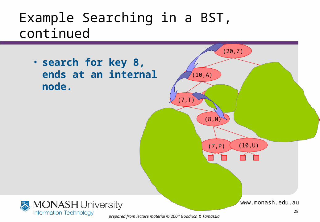
Example Searching in a BST, continued
• search for key 8, ends at an internal node.
(20,Z)
(37,P)(21,O)(14,J)
(7,T)
(35,R)(10,A)
(1,C)
(1,Q)
(5,G)(2,R)
(5,H)
(6,Y)(5,I)
(8,N)
(7,P)
(36,L)
(10,U)
(40,X)
www.monash.edu.au
29prepared from lecture material © 2004 Goodrich & Tamassia
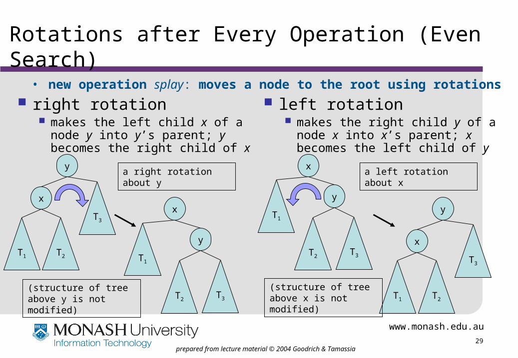
Rotations after Every Operation (Even Search)
• new operation splay: moves a node to the root using rotations right rotation
makes the left child x of a node y into y’s parent; y becomes the right child of x
left rotation makes the right child y of a node x into
x’s parent; x becomes the left child of y
y
x
T1 T2
T3
y
x
T1
T2T3
y
x
T1 T2
T3
y
x
T1
T2T3
(structure of tree above y is not modified)
(structure of tree above x is not modified)
a right rotation about y a left rotation about x

www.monash.edu.au
30prepared from lecture material © 2004 Goodrich & Tamassiaprepared from lecture material © 2004 Goodrich & Tamassia
Splaying: “x is a left-left grandchild” means x is a left child of its parent, which is itself a left child of its parent
p is x’s parent; g is p’s parent
is x the root?
stop
is x a child of the root?
right-rotate about the root
left-rotate about the root
is x the left child of the
root?
is x a left-left grandchild?
is x a left-right grandchild?
is x a right-right grandchild?
is x a right-left grandchild?
right-rotate about g, right-rotate about p
left-rotate about g, left-rotate about p
left-rotate about p, right-rotate about g
right-rotate about p, left-rotate about g
start with node x
no
yes
yes
yes
yes
yes
yes
no
no
yes zig-zig
zig-zag
zig-zag
zig-zig
zigzig
www.monash.edu.au
31prepared from lecture material © 2004 Goodrich & Tamassiaprepared from lecture material © 2004 Goodrich & Tamassia
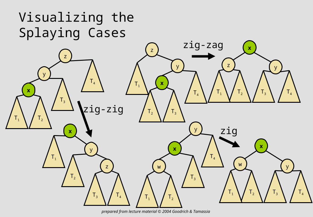
Visualizing the Splaying Cases
zig-zag
y
x
T2 T3
T4
z
T1
y
x
T2 T3 T4
z
T1
y
x
T1 T2
T3
z
T4
zig-zig
y
z
T4T3
T2
x
T1
zig
x
w
T1 T2
T3
y
T4
y
x
T2 T3 T4
w
T1
www.monash.edu.au
32prepared from lecture material © 2004 Goodrich & Tamassiaprepared from lecture material © 2004 Goodrich & Tamassia
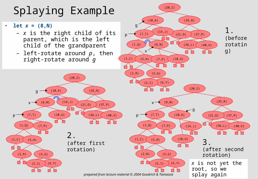
Splaying Example• let x = (8,N)
– x is the right child of its parent, which is the left child of the grandparent
– left-rotate around p, then right-rotate around g
(20,Z)
(37,P)(21,O)(14,J)
(7,T)
(35,R)(10,A)
(1,C)
(1,Q)
(5,G)(2,R)
(5,H)
(6,Y)(5,I)
(8,N)
(7,P)
(36,L)
(10,U)
(40,X)
x
g
p
(10,A)
(20,Z)
(37,P)(21,O)
(35,R)
(36,L) (40,X)(7,T)
(1,C)
(1,Q)
(5,G)(2,R)
(5,H)
(6,Y)(5,I)
(14,J)(8,N)
(7,P)
(10,U)
x
g
p (10,A)
(20,Z)
(37,P)(21,O)
(35,R)
(36,L) (40,X)
(7,T)
(1,C)
(1,Q)
(5,G)(2,R)
(5,H)
(6,Y)(5,I)
(14,J)
(8,N)
(7,P)
(10,U)
x
g
p
1.(before rotating)
2.(after first rotation) 3.
(after second rotation)
x is not yet the root, so we splay again
www.monash.edu.au
33prepared from lecture material © 2004 Goodrich & Tamassia
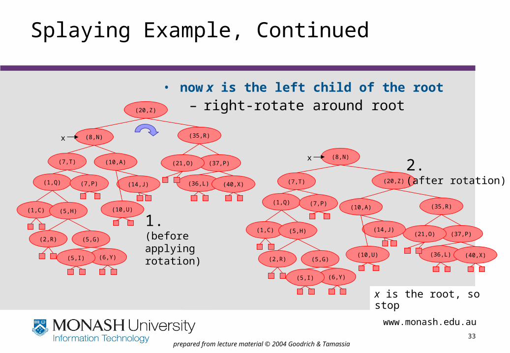
Splaying Example, Continued
• now x is the left child of the root
– right-rotate around root
(10,A)
(20,Z)
(37,P)(21,O)
(35,R)
(36,L) (40,X)
(7,T)
(1,C)
(1,Q)
(5,G)(2,R)
(5,H)
(6,Y)(5,I)
(14,J)
(8,N)
(7,P)
(10,U)
x
(10,A)
(20,Z)
(37,P)(21,O)
(35,R)
(36,L) (40,X)
(7,T)
(1,C)
(1,Q)
(5,G)(2,R)
(5,H)
(6,Y)(5,I)
(14,J)
(8,N)
(7,P)
(10,U)
x
1.(before applying rotation)
2.(after rotation)
x is the root, so stop
www.monash.edu.au
34prepared from lecture material © 2004 Goodrich & Tamassiaprepared from lecture material © 2004 Goodrich & Tamassia
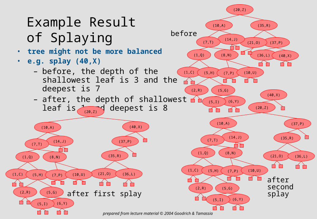
Example Result of Splaying
• tree might not be more balanced• e.g. splay (40,X)
– before, the depth of the shallowest leaf is 3 and the deepest is 7
– after, the depth of shallowest leaf is 1 and deepest is 8
(20,Z)
(37,P)(21,O)(14,J)
(7,T)
(35,R)(10,A)
(1,C)
(1,Q)
(5,G)(2,R)
(5,H)
(6,Y)(5,I)
(8,N)
(7,P)
(36,L)
(10,U)
(40,X)
(20,Z)
(37,P)
(21,O)
(14,J)(7,T)
(35,R)
(10,A)
(1,C)
(1,Q)
(5,G)(2,R)
(5,H)
(6,Y)(5,I)
(8,N)
(7,P) (36,L)(10,U)
(40,X)
(20,Z)
(37,P)
(21,O)
(14,J)(7,T)
(35,R)
(10,A)
(1,C)
(1,Q)
(5,G)(2,R)
(5,H)
(6,Y)(5,I)
(8,N)
(7,P)
(36,L)
(10,U)
(40,X)
before
after first splay
after second splay
www.monash.edu.au
35prepared from lecture material © 2004 Goodrich & Tamassia
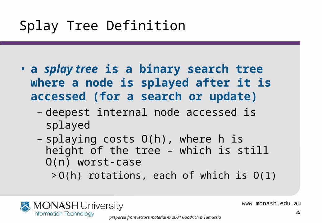
Splay Tree Definition
• a splay tree is a binary search tree where a node is splayed after it is accessed (for a search or update)– deepest internal node accessed is splayed– splaying costs O(h), where h is height of the tree
– which is still O(n) worst-case> O(h) rotations, each of which is O(1)
www.monash.edu.au
36prepared from lecture material © 2004 Goodrich & Tamassia
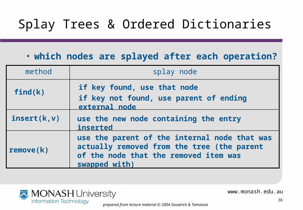
Splay Trees & Ordered Dictionaries
• which nodes are splayed after each operation?
use the parent of the internal node that was actually removed from the tree (the parent of the node that the removed item was swapped with)
remove(k)
use the new node containing the entry insertedinsert(k,v)
if key found, use that node
if key not found, use parent of ending external nodefind(k)
splay nodemethod

www.monash.edu.au
37prepared from lecture material © 2004 Goodrich & Tamassia
Amortized Analysis of Splay Trees
• “Amortized” means to balance the immediate cost of an operation with the future cost of further operations.
– total cost = immediate cost + future cost– (note: future costs could be negative!)
• Cost (run time) of each operation is proportional to the cost for splaying.
– splay at depth d is O(d), so is find, insert, delete > The immediate cost of an individual rotation are clear:
– Costs: zig = $1, zig-zig = $2, zig-zag = $2.
> splay at depth d performs at most d/2 zig-zig/zig-zag + 1 zig
• We only need to worry about splaying cost!

www.monash.edu.au
38prepared from lecture material © 2004 Goodrich & Tamassia
Amortized Analysis of Splay Trees
• To get a handle on the future cost we imagine that we maintain a virtual account at each node.
• We can pay into these accounts or withdraw from them.
• We will show that we can maintain a balance of $r(v) at each vertex v by paying a total of $O(log(n)) for each operation.
• Thus the amortized cost (run time) of each operation is O(log(n))
www.monash.edu.au
39prepared from lecture material © 2004 Goodrich & Tamassia
Invariant for the Analysis
• We define s(v) as the size of the subtree rooted in v (number of nodes) and
r(v)=log2(s(v)) “rank of v”
• Invariant: the balance at each vertex is $r(v).– wisely chosen so that
> the accounts are always positive > we don’t have to cheat by making an advance payment for an empty tree
ie that we do not start the amortization with accounts that have money in them
> we can show the amortized cost to be O(log n)
• The future cost of a rotation is the cost of maintaining this invariant.
www.monash.edu.au
40prepared from lecture material © 2004 Goodrich & Tamassia
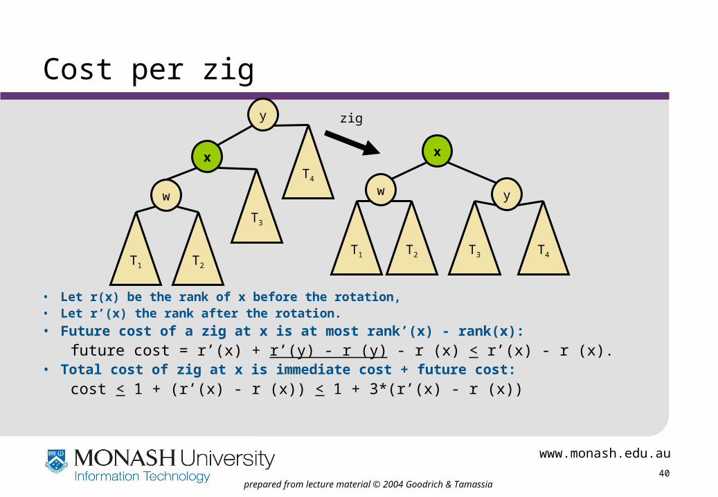
Cost per zig
• Let r(x) be the rank of x before the rotation,• Let r’(x) the rank after the rotation.
• Future cost of a zig at x is at most rank’(x) - rank(x):
future cost = r’(x) + r’(y) - r (y) - r (x) < r’(x) - r (x).• Total cost of zig at x is immediate cost + future cost:
cost < 1 + (r’(x) - r (x)) < 1 + 3*(r’(x) - r (x))
zig
x
w
T1 T2
T3
y
T4
y
x
T2 T3 T4
w
T1
www.monash.edu.au
41prepared from lecture material © 2004 Goodrich & Tamassia
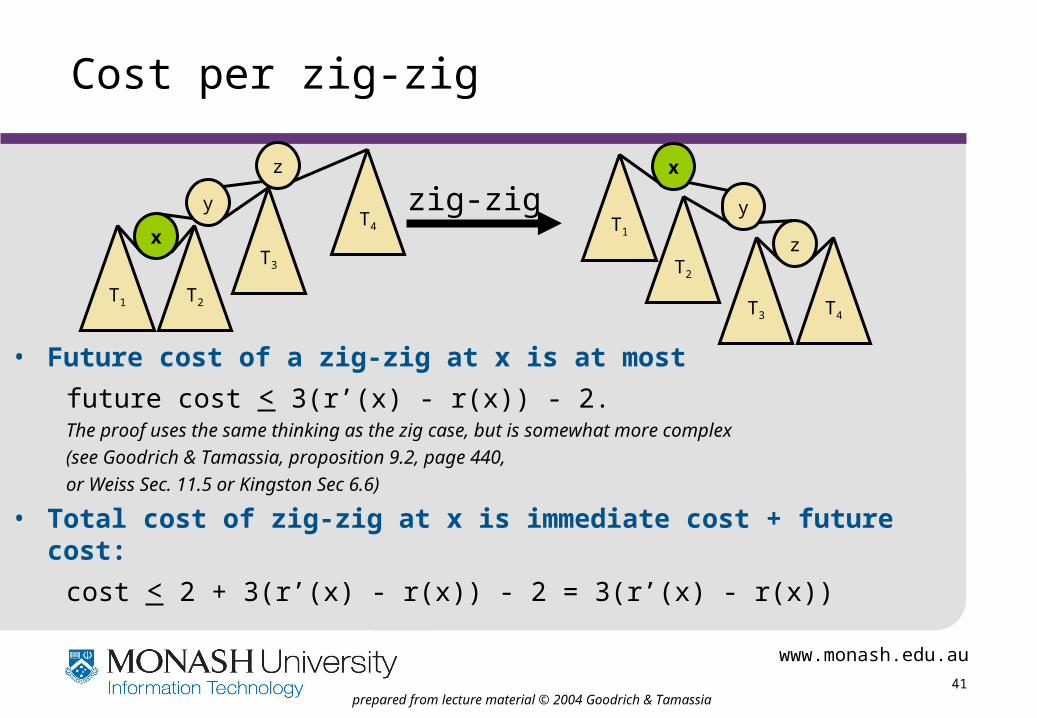
Cost per zig-zig
• Future cost of a zig-zig at x is at most
future cost < 3(r’(x) - r(x)) - 2.The proof uses the same thinking as the zig case, but is somewhat more complex
(see Goodrich & Tamassia, proposition 9.2, page 440,
or Weiss Sec. 11.5 or Kingston Sec 6.6)
• Total cost of zig-zig at x is immediate cost + future cost:
cost < 2 + 3(r’(x) - r(x)) - 2 = 3(r’(x) - r(x))
y
x
T1 T2
T3
z
T4
zig-zig y
z
T4T3
T2
x
T1

www.monash.edu.au
42prepared from lecture material © 2004 Goodrich & Tamassia
Cost per zig-zag
Same as cost for a zig-zig:• Future cost of a zig-zag or zig-zag at x is at most
future cost < 3(r’(x) - r(x)) - 2.• Total cost of zig-zig or zig-zag at x is immediate cost + future cost:
cost < 2 + 3(r’(x) - r(x)) - 2 = 3(r’(x) - r(x))
zig-zagy
x
T2 T3
T4
z
T1
y
x
T2 T3 T4
z
T1

www.monash.edu.au
43prepared from lecture material © 2004 Goodrich & Tamassia
Cost of Splaying (= cost of find)
• Splaying a node x means to rotate it all the way up to the root (m rotations)
• The last operation is a zig, all others are zig-zig or zig-zag.
• total splay cost is the sum of (m-1) zig-zig/zig-zag plus a final zig
• Let rm(x) be the rank of x just after rotation step m
cii=1
m
∑ = cii=1
m−1
∑ + cm
≤ 3(ri (x)−ri−1(x))[ ] +1+ 3(rm(x)−rm−1(x))i=1
m−1
∑= 3rm−1(x)−3r0 (x))[ ] +1+ 3rm(x)−3rm−1(x)= −3r0 (x)) +1+ 3rm(x)≤ 1+ 3rm(x)= 1+ 3logsm(x)= 1+ 3logn= O(logn)
www.monash.edu.au
44prepared from lecture material © 2004 Goodrich & Tamassia
Cost of Deletion
• The tree shrinks (by one node)
• the total variation of all r(t) is negative
• we don’t have to worry about any extra payment for maintaining the invariant

www.monash.edu.au
45prepared from lecture material © 2004 Goodrich & Tamassia
Cost of Insertion
• inserting node v increases the ranks of all of v’s ancestors
• let v=vo, v1 be its parent, and vi…vd all the ancestors on the way to the root.
• let n(vi) be the size of the subtree rooted at vi and r(vi) the corresponding rank (before insert)
• let n’(vi) and r’(vi) be the same values after the insert.
– n’(vi) = n(vi) +1
– n(vi) +1 ≤ n(vi+1)
• We have
• so the total variation is
www.monash.edu.au
46prepared from lecture material © 2004 Goodrich & Tamassia
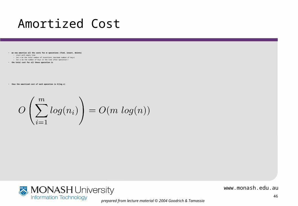
Amortized Cost
• we now amortize all the costs for m operations (find, insert, delete)– start with empty tree– let n be the total number of insertions (maximum number of keys)
– let ni be the number of keys in the tree after operation I
• the total cost for all these operation is
• thus the amortized cost of each operation is O(log n)
www.monash.edu.au
47prepared from lecture material © 2004 Goodrich & Tamassia
Performance of Splay Trees
• Thus, amortized cost of any splay operation is O(log n).
• Splay trees can adapt to perform searches on frequently-requested items much faster than O(log n) on average due to the “move-to-root” characteristics.
Top Related