


Languages
Pages
Legal


1
WIOD Socio‐Economic Accounts 2016
Sources and Methods
REITZE GOUMA
WEN CHEN
PIETER WOLTJER
MARCEL TIMMER
JANUARY 2018

2
1. Introduction
This document describes the sources and methods used for estimation of data on capital stocks and
employment variables for the 43 countries included in the WIOD 2016 database, called the Socio-Economic
Accounts (SEAs). The SEAs contain annual data (2000-2014) for 56 industries on:
Industry output, intermediate inputs, and value added
Price deflators for the above mentioned variables
Volume indices for the above mentioned variables
Capital stocks in current prices
Employment
Compensation of capital and labour
Note that this version of the WIOD Socio Economic Accounts no longer provides information on the
educational attainment of the labour force due to a lack of data, mostly for non-EU countries. Table 1 below
presents the full set of variables and their description, available in SEA 2016.
Table 1 Variables in the WIOD Socio-economic Accounts (SEA)
Output Millions of national currency
GO Gross output by industry at current basic prices
II Intermediate inputs at current purchasers' prices
VA Gross value added at current basic prices
Labour input Employment units
EMP Number of persons engaged (thousands)
EMPE Number of employees (thousands)
H_EMPE Total hours worked by employees (millions)
Compensation Millions of national currency
COMP Compensation of employees
LAB Total labour compensation
CAP Capital compensation
Capital input Millions of national currency
K Nominal capital stock
Indices 2010 = 100
GO_PI Price levels of gross output
II_PI Price levels of intermediate inputs
VA_PI Price levels of gross value added
GO_QI Gross output, volume indices
II_QI Intermediate inputs, volume indices
VA_QI Gross value added, volume indices
In this document the sources and methods for the construction are discussed for each group of variables,
excluding the output variables. Detailed information for the first group, the nominal values of Gross Output,
3
Intermediate Inputs and Value Added, is given in the documentation on the construction of the World Input
Output Tables (WIOTs) 20161.
Section 2 continues the discussion of the construction of the Labour Input and compensation variables. In
section 3 we turn to the construction methods of the capital stocks and in section 4 we discuss the sources
for the price indices from which the volume indices are derived. Section 5 presents the frequently used
mapping table between the ISIC Revision 3 industries from the SEA 2013 and the ISIC Revision 4 industries
from the SEA 2016.
2. Compensation and Labour Input
This section discusses the sources and methods for both the estimation of the labour and capital
compensation variables as well as labour input, since for many countries the calculation of total labour
compensation (LAB) is based on the employment data. First we start with a general discussion of the
sources and methods for European Countries, then we conclude with the country specific information for
the Non-EU countries.
Construction methods for EU28 countries and Norway
The source for the compensation and employment data is Eurostat. We take the variables from the ESA
2010 National Accounts for detailed industries (nama_10_a64 and nama_10_a64_e).2 We use the same
vintage as that used for the construction of the 2016 WIOD. To ensure that output and employment figures
are fully consistent, we use a stepwise approach to the construction of the compensation and employment
data. For example, to estimate total employment (EMP) we do not rely on the employment figures listed
in Eurostat directly, but instead estimate the ratio of VA to EMP from Eurostat and multiply by VA taken
from the 2016 WIOD. Note that this method will leave the levels of the variables listed in Eurostat
unaffected, unless in the construction of the (international) SUTs minor adjustments have been introduced
(see the WIOD 2016 documentation).
In this approach, the order in which the variables are estimated could matter. First, we estimate
total employment (EMP) based on the ratio of EMP to VA, as discussed above. Second, we multiply this
newly obtained value for EMP with the ratio of employees to total employment from Eurostat to obtain
the number of employees (EMPE) consistent with our output data. Third, we estimate the total hours
worked by employees (H_EMPE) based on the average annual hours of work for employees derived from
Eurostat. Lastly, we estimate the total compensation of employees (COMP) based on the ratio of COMP to
VA listed in Eurostat.
Extrapolation and disaggregation
If no (disaggregate) industry data is in available in Eurostat (nama_10_a64 and nama_10_a64_e) we rely
on the total economy figures from Eurostat instead (nama_10_lp_ulc and nama_10_gdp). We disaggregate
1 Sources and Methods for the WIOD 2016 SUT input files can be found in Timmer, M. P., Los, B., Stehrer, R. and de Vries, G. J. (2016), "An Anatomy of the Global Trade Slowdown based on the WIOD 2016 Release", GGDC research memorandum number 162, University of Groningen 2 Accessed: 15 January 2016

4
these figures, as well as the industry detail that is missing from the basic Eurostat tables to completely fill
the cells for all years and industries in the SEA.
In the disaggregation we estimate the missing values based on the parent’s value, i.e. the first
available industry, one level of aggregation above the current industry. For example, in the estimation of
total hours worked by employees (H_EMPE), we assume the average hours of work in the parent industry
is representative for the average hours of work in the industry for which data is missing. If data for a given
industry is unavailable for all years in the sample we directly rely on the level of the parent’s average hours
of work. If data is missing only for some years, we rely on the growth rate of the average hours of work for
the parent instead and link this to the level of the average hours of work that is available for this industry.
We then normalize to ensure that total hours of work for the industry and its siblings sum to the total hours
of work for the parent. We apply this procedure top-down, starting at the total economy level and working
our way down to fill the industries at the lowest level of aggregation in the SEA.
In our workflow, we first estimate the ratios discussed in the previous section for the industries
and years for which data is available in Eurostat. We then extrapolate these ratios over time, whenever
necessary, based on the total economy data from Eurostat. Lastly, we fill the missing values using the
disaggregation procedure discussed in the previous paragraph. The full matrix of ratios, say EMP/VA, can
then be used to calculate EMP for all years and industries by multiplying them with VA in the SEA.
Exceptions
In some (exceptional) cases we opted to discard the Eurostat data for specific industries if the resulting
ratios looked highly improbable. These exceptions are most likely the result of measurement issues, as it
concerns almost exclusively minor industries for smaller economies. For these observations we based the
ratios on the parent’s ratio instead (see previous section). In practice, we only applied this procedure for
the estimation of H_EMPE and only for four countries.
For Finland we discarded the average hours of work data listed in Eurostat for all years for the industry
codes A01, A02, and A03. For Cyprus and Malta, we discarded the average hours of work data for all the
lowest aggregates for all years.3 For Latvia we discarded all the average hours of work data below the total
economy level prior to 2008, to compensate for a clear break - most likely the result of a change in the SNA
- that occurs in the Latvian data between the years 2007 and 2008. In addition, we identified some outliers
in the Eurostat data which we dropped from the SEA and interpolated instead.4
3 i.e. industry codes A01, A02, A03, C16, C17, C18, C19, C22, C23, C24, C25, C29, C30, C31_C32, C33, E36, E37-E39, G45, G46, G47, H49, H50, H51, H52, H53, J58, J59_J60, K64, K65, K66, L68A, L68x, M69_M70, M71, M73, M74_M75, N77, N78, N79, N80-N82, Q86, Q87_Q88, R90-R92, R93, S94, S95, S96 4 We identified observations as outliers if the ratio has a z-score below -2.5 or above 2.5, but only if this was the case both across years (holding the industry constant) and industries (holding the year constant) for any given country. For the EMP/VA ratio we identified 0 outliers, for the EMPE/EMP ratio we identified 11 outliers (0.05% of the sample), for the H_EMPE/EMPE ratio we identified 66 outliers (0.27% of the sample, and for the COMP/VA ratio we identified 0 outliers.
5
Derivation of total Labour compensation (LAB)
As a general method for deriving values for total labour compensation (LAB) we assume that self-employed
persons in the industry receive the same average wages as employees. When explicit information on Mixed
Income (MIXINC) is available from Use tables, we calculate the share of MIXINC in VA, and add it to the
share of COMP in VA to derive an upper limit for LAB.5 This upper limit is then extended backwards and
forwards for years where MIXINC is not available, using the growth of LAB derived using the general
method. The final value for LAB is the minimum value of the upper limit and the general method.
5 MIXINC is available for Belgium, Czech Republic, Estonia, Hungary, Netherlands, Poland, Romania, and Slovenia from 2010 onwards.

6
Table 2 industry coverage employment variables for EU28 and Norway
EMP EMPE H_EMPE COMP
Country level years level years level years level years
AUT Austria a64 15 a64 15 a64 15 a64 15 BEL Belgium a64 14 a64 15 a21 15 a64 14 BGR Bulgaria a64 14 a64 15 a21 15 a64 14 CYP Cyprus a64 14 a64 15 a21 15 a64 14 CZE Czech Republic a64 15 a64 15 a64 15 a64 15 DEU Germany a64 14 a64 14 a21 14 a64 14 DNK Denmark a64 15 a64 15 a64 15 a64 15 ESP Spain a64 14 a64 14 a64 14 a64 14 EST Estonia a64 15 a64 15 a64 15 a64 15 FIN Finland a64 15 a64 15 a64 15 a64 15 FRA France a64 14 a64 14 a21 14 a64 14 GBR United Kingdom a64 15 a64 15 a21 15 a64 15 GRC Greece a64 15 a64 15 a64 15 a64 15 HRV Croatia a64 7 a64 7 a64 7 a64 14 HUN Hungary a64 15 a64 15 a64 5 a64 15 IRL Ireland a64 15 a64 15 a64 15 a64 15 ITA Italy a64 14 a64 14 a21 15 a64 14 LTU Lithuania a64 14 a64 14 a21 14 a64 14 LUX Luxembourg a38 15 a38 15 a38 15 a38 15 LVA Latvia a64 14 a64 14 a10 7 a64 14 MLT Malta a64 15 a64 15 a21 15 a64 15 NLD Netherlands a64 15 a64 15 a64 15 a64 15 NOR Norway a64 13 a64 13 a64 13 a64 14 POL Poland a64 10 a64 15 a64 15 a64 10 PRT Portugal a64 14 a64 14 a21 14 a64 14 ROU Romania a64 14 a64 14 a64 14 a64 14 SVK Slovakia a64 15 a64 15 a64 15 a64 15 SVN Slovenia a64 15 a64 15 a64 15 a64 15 SWE Sweden a64 14 a64 14 a64 14 a64 14
Notes: the ‘level’ column indicates the industry coverage used in the construction of the SEA; a64 represents full coverage. The ‘years’ column shows the number of years for which this industry detail is available; 15 represents full coverage.
Sources: Eurostat, tables nama_10_a64 and nama_10_a64_e, accessed: 15 January 2016

7
Construction methods for Non-EU countries
For Non-EU countries there is no standard source of information, therefore we discuss the sources for each
individual country. Whenever we use the ratio of two variables from the WIOD SEA 2013, we use the
mapping table given in section 5 to map ISIC Rev. 3 sectors to the ISIC Rev. 4 industries.
Australia
EMP, EMPE, H_EMPE are taken from OECD National Accounts (OECD NA), full industry detail is
available for these labour input variables.
Data on VA and COMP are also taken from OECD NA for 18 broad sectors. The COMP/VA ratios at
the broad sector level are applied to the detailed industries in their respective aggregates.
We apply the same method as for the European countries in order to determine total LAB.
Brazil
COMP is available from the official SUTs for the years 2010-2013 that are used for the estimation
of the time series SUTs in WIOD 2016, and is fully consistent with the VA data in the WIOTs.
Back-casts for COMP to 2000 and extrapolations to 2014 are calculated using the growth of COMP
from SUTs. We use the information provided in the annual supply and use tables that directly
underlies the national accounts, as published by Brazil’s statistical office (IBGE)6. We use the
detailed SUTs for the years 2010-2014 and extrapolate backwards to 2000 using the less detailed
SUTs for the years 2000-2009. The concordance is equal to that underlying the time series SUTs for
the 2016 WIOD release.
The same SUTs also provide information on EMP and VA for the whole period. The ratios have been
applied to the VA data from the WIOTs in order to obtain EMP.
The share of EMPE in EMP are estimated using PNAD microdata.
H_EMPE is calculated using the average hours worked from the SEA 2013 data.
IBGE also provides Mixed Income (MIXINC) in the annual SUTs. We use this information in the same
way as for the European countries in order to determine the values for total LAB.
Canada
Information on COMP, VA, EMP, EMPE, and H_EMPE is available from OECD national accounts
(OECD NA) for all ISIC Rev. 4 industries.
COMP and VA are available from 2007 onwards, the ratio of COMP/VA has been extrapolated
backwards to 2000 using the ratios from SEA2013.
From the OECD data we have calculated and applied EMP/VA to the VA from the WIOTs for 2007-
2014. Before 2007 we have extrapolated the data for EMP using the growth of the EMP levels from
OECD NA.
From the resulting data for EMP we have applied the ratio EMPE/EMP from OECD NA to calculate
EMPE values for each industry.
6 https://downloads.ibge.gov.br/downloads_estatisticas.htm

8
The employment variables are available for 2000-2013. The ratios of labour input versus VA that
are used have been assumed constant at the 2013 levels for 2014.
We have applied average hours worked from OECD NA for employees to estimate total hours
worked by employees for each industry.
STATCAN provides information on the wages of both employees and the self-employed for 62
NAICS industries which are mapped to 42 ISIC Rev. 4 industries. 7 For these industries we calculate
the ratio of LAB/COMP and apply this to the industry COMP values calculated above in order to
estimate total LAB for each in industry.
Switzerland
We use the data on Jobs and hours from Nathani et al. (2016).8 Jobs are taken as persons engaged.
We apply EMP/VA ratios of aggregate sectors using VA from the SUTs, to industries that were
missing from the Nathani et al. (2016) data in Utilities, Transportation, Information and
Communication, and Business services.
We used average hours worked derived from the Nathani et al. (2016) data, and multiplied this by
the calculated persons engaged.
We use the ratios of employees over total persons engaged from the German 2013 SEA to calculate
employees, and the same was done to estimate hours worked by employees.
Data is available from Eurostat Structural Business Statistics (SBS) on labour cost, turnover and
Value Added at Factor Cost, for detailed industries. The ratio of labour cost over value added at
factor cost is taken as the LAB share. These data are available for 2009-2014.
The data from SBS does not contain information for the following sectors: Agriculture (A),
Manufacture of coke and refined petroleum products (C19), Water Transport (H50), Air Transport
(H51), Warehousing and support activities for transportation (H52), Financial services (K), Public
Administration (O), Education (P), and Human health and social work activities (Q). For these
industries the LAB shares of Germany were used.
For the period 2000-2008 the LAB shares are extended backwards from the 2009 values using the
growth in the German shares.
For the Mining sector (B), we keep the shares constant at the 2009 level for the 2000-2008 period,
since the output for this industry remains very stable, which is not the case for the German
industry, making the pattern of the German LAB shares for this industry not representative for
Switzerland.
We calculate COMP backwards from total labour compensation by assuming the employees earn
the same hourly wage as the self-employed.
7 STATCAN table 0380024 8 The data for Switzerland has been constructed in close cooperation with from Rütter Soceco AG and we are grateful to Carsten Nathani for advice and help. The underlying data construction work is described in: Nathani, C., Hellmüller, P., Schwehr, T. (2016): Adaptation of Swiss data for the World Input-Output Database. Technical report. Rütter Soceco, Rüschlikon.

9
China
Data on productivity (VA/EMP) is taken from the China Statistical Yearbooks (CSY) for three broad
sectors. This information is used to estimate total employment for these three sectors in the SEA,
by multiplying it by aggregate sector VA from the WIOTs.
The employment figures are further broken down by industry using the China Industrial
Productivity (CIP) database, which provides information on output and labour for 29 industries,
which are mapped to the ISIC Rev. 4 industries in WIOD. From the CIP data we estimate productivity
levels. The CIP data is only available up to 2010, therefore the productivity levels are extrapolated
using the productivity growth of the CSY data by three broad sectors. The resulting time series of
productivity are multiplied by VA from the WIOTs, to obtain a first estimate of EMP for detailed
ISIC Rev. 4 industries.
The EMP levels for detailed industries are normalized to the EMP levels derived from the CSY data
by the three broad sectors.
For China no separate information is available on labour input by employees.
LAB shares in VA are derived from labour compensation provided in the input-output tables. Before the
first Economic Census in 2004, the income of self-employed and their employees are included in labour
compensation (NBS, 2003). While profits related to owners (informal entrepreneurs) should be part of
gross operating surplus, we consider the labour compensation in the input-output tables before 2004
closest to the definition of labour compensation in value added. After the economic census, two changes
in the income GDP accounting method introduce a break in the labour share time series by industry (Bai
and Qian, 2010). First, profits of state-owned and collective-owned farms are included in labour
compensation, introducing an upward break in the agricultural labour shares. Second, income of self-
employed owners is subsequently included in gross operating surplus.
We use the adjustment factors for these changes at the sector level in Bai and Qian (2010) for the 2007
and 2012 IOT (except for H53, O84, P85, and Q), to arrive at consistent time series that correspond most
closely to the definition of labour shares before the 2004 Economic Census. We estimate LAB shares in VA
based on the 2002, the 2007 and the 2012 IOT. Years in between are interpolated. 2000-2001 labour shares
are equal to 2002 and 2013-2014 labour shares are equal to 2012. The derived LAB shares are multiplied
by VA from the WIOTs, converted back to Yuan, to obtain LAB.
Indonesia
The ratios for COMP/VA, LAB/VA, EMP/VA, EMPE/EMP, and H_EMPE/EMPE are taken from the
SEA 2013 data and have been used together with VA from WIOD 2016 to estimate values for
COMP, LAB, EMP, EMPE, and H_EMPE.
The ratios are kept constant after 2009.
India
The ratios for EMP/VA, LAB/VA, COMP/VA, EMPE/EMP, are taken from India KLEMS.9 Data is
available for 27 sectors (ISIC Rev. 3), these are mapped to WIOD industries. The same mapping is
9 https://www.rbi.org.in/Scripts/PublicationReportDetails.aspx?UrlPage=&ID=85
10
used as for the external output series in the SUTs. The last available year is 2011. Shares after
2011 are set equal to their 2011 values.
Average hours worked by employees is taken from SEA 2013, and held constant after 2009.
Japan
We use Nominal Labour cost and Value Added from the JIP 2015 database to determine LAB.
Data is available up to 2012, the share of LAB in VA is assumed to be constant afterwards.
Data for EMP and H_EMP are also taken from JIP 2015.
EMP/EMPE ratios are taken from OECD STAN, EMP/VA ratios are updated for 2013 and 2014
using the trends in the STAN ratios. Data for some 33 ISIC Rev. 4 sectors are available from STAN,
so the ratios of aggregate sectors are applied to detailed industries when STAN data is missing.
Average hours worked by self-employed is assumed to be the same as for employees.
COMP is reverse calculated from LAB assuming the self-employed earn the same wages as
employees.
Korea
For Korea there are Use tables available for 2010-2014 for detailed (82) industries, as well as
accompanying information on hours worked for both Employees and total persons engaged. The
industries are mapped to the industries in the WIOTs.
LAB values are calculated in the standard way for 2010-2014, by assuming that the self-employed
receive the same hourly wages as employees.
In order to derive estimates for 2000-2009 there are two additional sources that were used: The
information from the previous WIOD 2013 release in the old SNA and industry classification and
information from OECD for 19 distinguished aggregate sectors. The OECD data is available for
2004-2013.
For all non-manufacturing sectors the shares are cast back using the growth in the OECD shares.
Aggregate industries from OECD are mapped to detailed WIOT industries.
For the manufacturing industries the shares in 2009 are assumed to match the 2010 shares. From
2009 back to 2000 the growth of the SEA 2013 LAB shares are used to cast back the series.
For the period 2000-2003 the approach for manufacturing industries is applied to all industries
For the labour input variables the detailed SUT data from the Bank of Korea for 2010-2014 is
taken as a baseline for employment ratios (EMP/VA, EMPE/EMP, H_EMP/EMP, H_EMPE/EMPE).
These ratios have been back-cast using data from the Korean Industrial Productivity (KIP)
database, which provides data for 2000-2012 for the SEA 2013 industries.
The resulting ratios have been multiplied by VA from the WIOD SUTs to obtain the levels of
employment.
COMP has been estimated by calculated backwards from LAB for each of the 56 ISIC Rev. 4 WIOD
industries.
The ratios of average hours worked (H_EMP/EMP, H_EMPE/EMPE) for the agricultural sector
from the detailed BOK SUTs were implausibly low. Therefore we reverse the procedure for the
ratios of the agricultural sector, taking the levels of the KIP data and extending it beyond 2012
using the trend of the BOK SUT ratios.

11
Mexico
From the data published by Mexico’s statistical office (INEGI) in its productivity report (Mexico KLEMS) we
use value added, compensation of employees, hours worked, and persons engaged by industry. 10
Levels of EMP and COMP are calculated through their ratios over VA, and multiplied by VA from the WIOD
2016. It should be noted that compensation as a share in value added is very low for several sectors, in
particular agriculture. A large part of informal labour income is included in gross operating surplus. Using
previous estimates of the share of employees in total employment (documented in the SEA 2013) we
estimate the labour income as:
𝐿𝐴𝐵𝑐𝑖𝑡 = ((𝐶𝑂𝑀𝑃𝑐𝑖𝑡 /𝐸𝑀𝑃𝐸𝑐𝑖𝑡) ∗ (𝐸𝑀𝑃𝑐𝑖𝑡 − 𝐸𝑀𝑃𝐸𝑐𝑖𝑡)) + 𝐶𝑂𝑀𝑃𝑐𝑖𝑡
Where LAB is labour income, COMP is compensation of employees, EMP is persons engaged, and EMPE is
employees. Subscript c refers to Mexico here, i to each of the 56 industries distinguished and t to year
(2000 to 2014). EMP/EMPE ratios from SEA 2013 are applied for the estimation of EMPE and H_EMPE.
Russia
VA, EMP, H_EMP, and LAB, are directly available from WorldKLEMS v2017, provided by National
Research University Higher School of Economics, for 35 ISIC Rev. 3 industries. We use the ratios
of these variables over VA, and multiply them with VA from the WIOD 2016. The ISIC Rev. 3
industries are mapped to the 56 ISIC Rev. 4 industries in the SEA according to the mapping table
in section 5.
We apply H_EMP/H_EMPE and EMP/EMPE ratios to calculate employment for employees, using
SEA13 data (available up to 2009).
COMP is inversely derived from LAB, by assuming the average hourly wage rate is the same for
employees and self-employed persons.
Turkey
The ratios for COMP/VA, LAB/VA, EMP/VA, EMPE/EMP, and H_EMPE/EMPE are taken from the
SEA 2013 data and have been used together with VA from WIOD 2016 to estimate values for
COMP, LAB, EMP, EMPE, and H_EMPE.
The ratios are kept constant after 2009.
Taiwan
The base line data for total persons engaged stems from the Taiwanese Statistical Yearbook (TSY)
for the year 2000-2014.
The Chinese Statistical Yearbook (CSY) provides the distribution of labour across 14 broad sectors
of the economy. This is used to distribute the total economy values from the TSY.
To further break down the labour statistics for detailed industries we use data from the
Taiwanese Payroll Statistics (TPS), which provides information on total employees, average
monthly hours worked and average monthly wages, for 113 industries. Each of these industries
has been mapped to the WIOD industries, as well as the 14 broad sectors distinguished by the
Chinese Statistical Yearbook. The payroll statistics do not cover Public Administration and Defense
10 See http://www3.inegi.org.mx/sistemas/tabuladosbasicos/tabniveles.aspx?c=33687

12
(O84), or the agricultural sector (A). Furthermore wholesale and retail trade (G) is not further
broken down. The same holds for the aggregate of the Scientific research and development
industry (M72) and the Other professional, scientific and technical activities; veterinary activities
(M74_M75). The data for A, G and M72+M74_M75 is further broken down using Value Added
shares.
For the available industries from the TPS, we take the total number of employees as given and
aggregate them to the 14 broad sectors from CSY. For Agriculture (A) and Education (P85) we
apply the ratio of employees to total persons engaged from SEA 2013 to estimate the number of
employees. For Public Administration and Defense (O84) we assume that all persons engaged are
employees.
From the calculated Persons Engaged (EMP) and Employees (EMPE) statistics we compute the
ratios for the 14 broad sectors. In cases these ratios exceed 100%, the value of EMP is taken for
EMPE.
We calculate the average hours worked by employees from the TPS data on average monthly
hours worked by multiplying the data by 12 and then by the respective industries’ number of
employees and aggregating. Average annual working hours for the agricultural sector are derived
from the Man Power Utilization survey. For Public Administration and Defense (O84) we assume
average working hours to be the same as the average for other services which includes the
following sectors:
o Real eatate (L)
o Business services (M-N)
o Human health and social work activities (Q)
o Other Other service activities (R_S)
o Activities of households as employers; undifferentiated goods- and services-producing
activities of households for own use (T)
In order to estimate the compensation of employees we take the share of COMP in VA from the
official SUTs in 2006 and 2011 and linearly interpolate the shares between these years. Before
2006 and after 2011 the COMP shares are held constant.
Labour compensation (LAB) are estimated in the standard way, by assuming the self-employed
persons receive the same average wages as employees.
Note:
The COMP data as a percentage of VA is taken from the SUTs. However, the employment levels are
taken from the TSY, while the industry distribution is taken from first the CSY by 14 broad sectors and
then from the TPS by detailed industries. This can create a mismatch in the distribution pattern of
employees and the compensation of employees, which can result in extreme values for the
estimation of LAB, especially when EMPE/EMP ratios are low, as is the case for the agricultural sector.
Average wages per employee can also be either over- or underestimated, due to this distribution
mismatch. We have chosen for this method since it provides a clear link between COMP and VA from
the Taiwanese National Accounts statistics and there is no harmonized source where values for
labour input, labour compensation and output are given.

13
United States
We take COMP data directly from the BEA USE tables which underlie the time series SUTs in the
WIOD 2016. We use the same mapping tables and as such, these values are fully consistent with
VA.
Information on persons engaged and employees and VA is collected from the BEA for detailed
NAICS industries, which are mapped to the ISIC Rev. 4 industries. We take the ratio of EMP/VA
and EMP/VA from the BEA data and multiply it by VA to estimate EMP for each industry. We
apply the BEA EMPE/EMP ratios to the estimated EMP values to obtain EMPE values for the ISIC
Rev. 4 industries.
Reported total persons engaged from the BEA includes FTE employees, rather than persons,
therefore total employment numbers have been recalculated.
Mixed income is available as 'Nonfarm Proprietors' Income by Industry' for 21 aggregate sectors,
which was used in the following way:
o The COMP/VA ratio is calculated as the lower limit and (MIXINC+COMP)/VA as the upper
limit for aggregate sectors.
o The ratio of the upper limit divided by the lower limit, defined as COMP/VA, is computed
for the same aggregate sectors.
o These ratios are applied to the lower limit (COMP/VA) for the detailed 56 ISIC Rev. 4
industries to compute the upper limit for the LAB as a percentage of VA.
o The final estimation of LAB for each industry is taken as the minimum value of the upper
limit times VA and LAB calculated through the standard method where the self-employed
are assumed to have equal average annual wages as employees (COMP/EMPE*EMP).
H_EMPE data is available from the BEA for 16 broad sectors. These have been divided by the BEA
data on number of employees, and these ratios have been applied to detailed industries and
multiplied by the calculated number of employees in each industry.
14
3. Capital Input - Construction of capital stock estimates
Depending on country-specific data availability, various methods are employed in constructing the capital
stock estimates for WIOD 2016 release. This appendix describes in detail the sources and methods used for
each of the 43 countries covered in WIOD 2016. The resulting annual capital stock estimates are classified
by 56 ISIC Rev.4 industries. The data are expressed in nominal local currency units over the period 2000-
2014. The capital stock series correspond to fixed assets as defined in the guidelines of System of National
Accounts 2008 (SNA08), with some exceptions (see table 3 for an overview).
Data Availability
Broadly speaking, among the 43 countries that we cover four different groups can be identified during the
data construction process in terms of their data availability:
1. Countries for which capital stock data is available in current or constant prices and by detailed ISIC
Rev.4 industry classification adhering to the SNA08 definitions.
2. Countries for which capital stock data is available either in current or constant prices, but in a
different industry classification than ISIC Rev.4 (e.g. ISIC Rev.3 or country-specific industry
classification). These data adhere either to SNA08 or SNA93 definitions.
3. Countries for which no information on capital stocks can be found but gross fixed capital formation
(GFCF) data are available at different levels of industry detail. The industry classification and SNA
definitions are country dependent in this case.
4. Countries for which no capital stock or GFCF data can be found at the industry level. The only
information can be obtained is their aggregate GFCF series at the total economy level from the UN
National Accounts database (UNNA), e.g. Indonesia and Turkey.
Estimation Methods
For the first two groups of countries we can use the data directly if industry detail is available for the 56
ISIC Rev.4 industries. When the capital stock data is available at a more aggregate industry level, we split
the aggregate sectors using either the value-added shares split method or the so-called hybrid split method,
see below for a more detailed explanations. For countries that do not have capital stocks data readily
available, an extra step of building up the stock estimates using perpetual inventory method (PIM) is
required. We do so by using the capital stocks data provided in the WIOD social economic accounts 2013
release (SEA 2013) as the starting point and we update the SEA 2013 capital stocks based on PIM from 2009
onward up to 2014. This is termed the SEA 2013 updated method which we turn to discuss in more detail
below. Note, that in the case of Switzerland and Croatia, for each industry and year, we estimated the
capital stock using nominal capital stock to value added ratios (K/VA) from an economically similar country,
i.e. Germany and Spain, respectively. Other deviations from the general methodology can be found in the
country specific notes.
Value-added shares split method
One of the major hurdles in deriving capital stock estimates for the WIOD 2016 release is that the nominal
capital stock or investment data we extract from external sources are frequently available at a more
aggregated industry level than the required 56 ISIC Rev.4 industries. As a prime solution to split the
15
aggregate estimates into more detailed industries we rely on industry valued added shares from the WIOD
2016 release.
For example, when capital stock data is available only for the aggregate agricultural sector as a whole, we
split it into three detailed ISIC Rev.4 agricultural industries (i.e. 𝐴01 𝐴02 and 𝐴03) that are consistent with
the WIOD 2016 release. We use the corresponding value-added shares in total agriculture (i.e. 𝑆ℎ𝑎𝑟𝑒𝑖,𝑡𝑉𝐴 =
𝑉𝐴𝑖,𝑡
𝑉𝐴𝑡) as weights and then multiply these weights by the aggregate nominal capital stock (K𝑖,𝑡 = 𝐾𝑡 ×
𝑆ℎ𝑎𝑟𝑒𝑖,𝑡𝑉𝐴). Based on this VA share split method, estimates for investments or capital stocks at the 56
detailed ISIC Rev.4 industries can be obtained.
However, a major drawback of this method is that it assumes the same capital intensity for all industries in
the aggregate sector that needs to be split. This can be quite problematic for the manufacturing sector
where the underlying industries can differ considerably in terms of their capital intensity. For this reason,
when only very aggregate data are available (especially in case of the manufacturing sector), we use an
additional step to include detailed industry level information on capital intensity from WIOD 2013 in the
hybrid split approach which we discuss below.
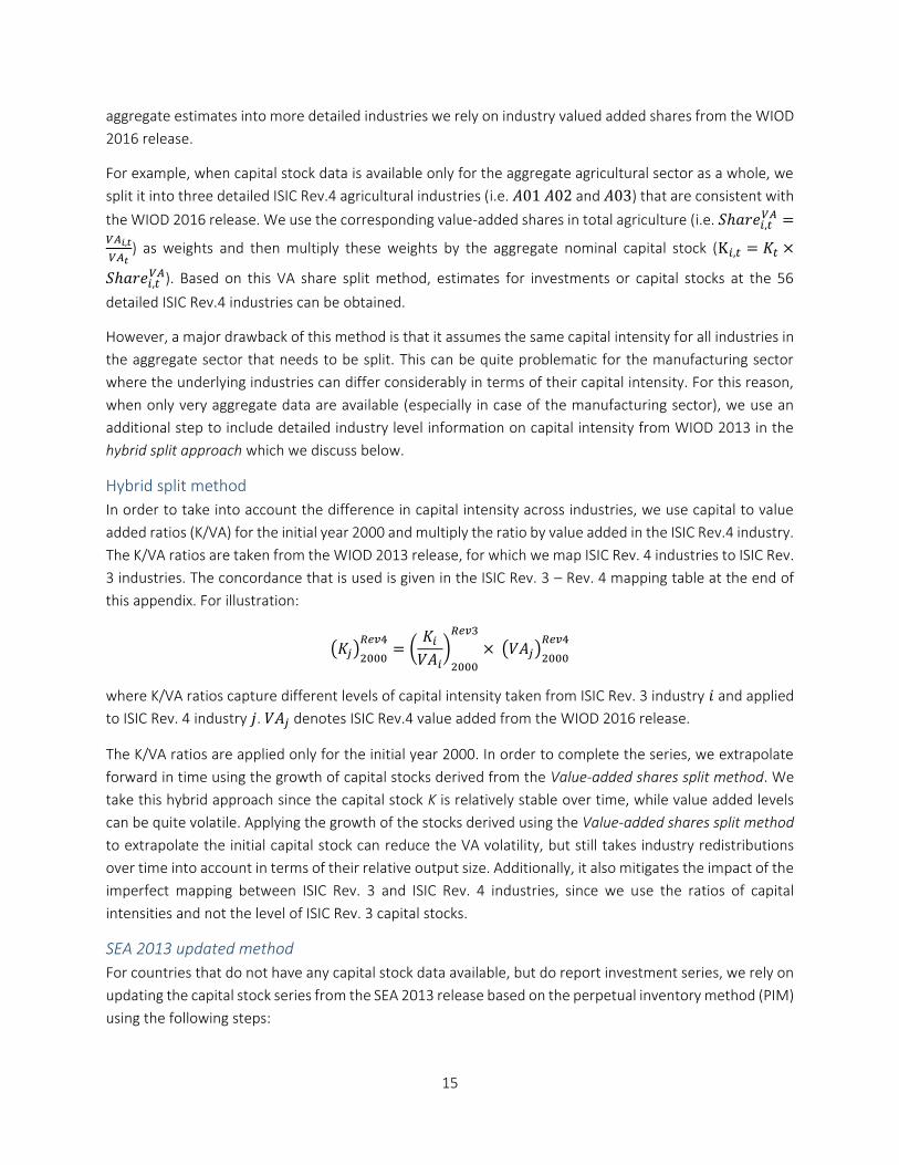
Hybrid split method
In order to take into account the difference in capital intensity across industries, we use capital to value
added ratios (K/VA) for the initial year 2000 and multiply the ratio by value added in the ISIC Rev.4 industry.
The K/VA ratios are taken from the WIOD 2013 release, for which we map ISIC Rev. 4 industries to ISIC Rev.
3 industries. The concordance that is used is given in the ISIC Rev. 3 – Rev. 4 mapping table at the end of
this appendix. For illustration:
(𝐾𝑗)2000
𝑅𝑒𝑣4= (
𝐾𝑖
𝑉𝐴𝑖)
2000
𝑅𝑒𝑣3
× (𝑉𝐴𝑗)2000
𝑅𝑒𝑣4
where K/VA ratios capture different levels of capital intensity taken from ISIC Rev. 3 industry 𝑖 and applied
to ISIC Rev. 4 industry 𝑗. 𝑉𝐴𝑗 denotes ISIC Rev.4 value added from the WIOD 2016 release.
The K/VA ratios are applied only for the initial year 2000. In order to complete the series, we extrapolate
forward in time using the growth of capital stocks derived from the Value-added shares split method. We
take this hybrid approach since the capital stock K is relatively stable over time, while value added levels
can be quite volatile. Applying the growth of the stocks derived using the Value-added shares split method
to extrapolate the initial capital stock can reduce the VA volatility, but still takes industry redistributions
over time into account in terms of their relative output size. Additionally, it also mitigates the impact of the
imperfect mapping between ISIC Rev. 3 and ISIC Rev. 4 industries, since we use the ratios of capital
intensities and not the level of ISIC Rev. 3 capital stocks.
SEA 2013 updated method
For countries that do not have any capital stock data available, but do report investment series, we rely on
updating the capital stock series from the SEA 2013 release based on the perpetual inventory method (PIM)
using the following steps:

16
1. We convert their SEA 2013 investment series from ISIC Rev.3 (35 industries) to ISIC Rev.4 (56
industries) for the period 2000-2008 using the Value-added shares split method.
2. We estimate the 2000-2008 capital stock series from the WIOD 2013 data using the Hybrid split
method.
3. From the external investment data, we calculate Investment to Value Added ratios (I/VA) at the
level at which the data is available.
4. For the investment data by 56 ISIC Rev. 4 industries calculated in the first step, we also calculate
the I/VA ratios in 2008 and update these with the growth of the ratios from step 3. We use an
industry mapping of the domestic industries to the ISIC Rev. 4 industries that is dependent on the
available information for the country. In some cases, only total economy investment and output
data are available.
5. The extended I/VA ratios for the 56 ISIC Rev. 4 industries are multiplied by VA series from the WIOD
2016 release to estimate the investment series for all industries.
6. We extend the capital stocks calculated in step 2 using the PIM method for 2009-2014.
Note, the rate of depreciation that we use in PIM is based on the year- and industry-specific geometric
depreciation rates for Spain (obtained from the EU KLEMS database December 2016 revision), which are
calculated using each assets’ nominal capital stock as weights. These rates take into account the differences
in the composition of capital assets both across industries and over time. Moreover, in order to apply the
PIM-method the data on investments and stocks needs to be denoted in constant base year prices. From
the WIOD 2013 data the investment price deflators are available. For countries that have no investment
price deflators available from the external source, we use a total economy capital stock deflator calculated
from the Penn World Table, which excludes the price movements for Residential Structures.

17
Table 3 Overview of Capital Stock construction methods
Country Approach SNA Main data sources
1 AUS Hybrid 2008 OECD NA 2 AUT Directly obtained 2008 EUROSTAT 3 BEL VA shares 2008 EUROSTAT 4 BGR SEA 2013 updated 1993 EUROSTAT, EUKLEMS 5 BRA SEA 2013 updated 1993 UNNA, WIOD SEA2013 6 CAN VA shares 2008 OECD NA 7 CHE K/VA ratio of DEU 2008 WIOD 2016 8 CHN SEA 2013 updated 1993 China statistical yearbook 9 CYP SEA 2013 updated 1993 EUROSTAT 10 CZE Directly obtained 2008 EUROSTAT 11 DEU Directly obtained 2008 OECD NA/STAN, EUROSTAT 12 DNK Directly obtained 2008 EUROSTAT 13 ESP VA shares 2008 EU KLEMS 14 EST Hybrid 2008 EUROSTAT 15 FIN Directly obtained 2008 EUROSTAT 16 FRA VA shares 2008 OECD NA, EUROSTAT 17 GBR Directly obtained 2008 EUROSTAT 18 GRC Directly obtained 2008 OECD NA, EUROSTAT 19 HRV K/VA ratio of ESP 2008 WIOD 2016 20 HUN Hybrid 2008 EUROSTAT 21 IDN SEA 2013 updated 1993 UNNA, WIOD SEA2013 22 IND VA shares 1993 World KLEMS 23 IRL Hybrid 2008 OECD NA 24 ITA VA shares 2008 EUROSTAT 25 JPN Directly obtained 1993 REITI JIP database 26 KOR VA shares 1993 World KLEMS 27 LTU Hybrid 2008 EUROSTAT 28 LUX VA shares 2008 EUROSTAT 29 LVA SEA 2013 updated 1993 EUROSTAT 30 MEX VA shares 1993 NISG 31 MLT SEA 2013 updated 1993 EUROSTAT 32 NLD VA shares 2008 EUROSTAT 33 NOR VA shares 2008 EUROSTAT 34 POL Hybrid 2008 EUROSTAT 35 PRT Hybrid 1993 EUROSTAT 36 ROU Hybrid 1993 EUROSTAT 37 RUS Hybrid 1993 World KLEMS 38 SVK Directly obtained 2008 EUROSTAT 39 SVN Hybrid 2008 EUROSTAT 40 SWE VA shares 2008 EUROSTAT 41 TUR SEA 2013 updated 1993 UNNA, WIOD SEA2013 42 TWN SEA 2013 updated 1993 National development council 43 USA Directly obtained 2008 BEA

18
Country-specific notes
1. AUS - Australia
We obtain SNA08 total capital stocks from OECD national accounts for 20 sectors.
We use capital stock to value added ratios (K/VA) from SEA 2013 for detailed manufacturing sectors
to estimate an initial capital stock for year 2000. For all other sectors, we apply VA shares directly
to the reported stock levels.
For the detailed manufacturing industries, we extrapolate the estimated initial stocks using the
growth of the stock series obtained by applying VA shares. We then renormalize the total
manufacturing level of stocks to those reported by OECD NA.
2. AUT - Austria
SNA08 / ISIC Rev. 4 capital stocks for 56 industries are directly taken from EUROSTAT.
3. BEL - Belgium
SNA08 / ISIC Rev. 4 capital stocks are available at the A38 level from EUROSTAT.
Stocks in current prices are split using VA shares.
4. BRA - Brazil
There are no capital stocks data available for Brazil, therefore, we update the SEA 2013 capital
stocks using the SEA 2013 updated method.
We use the investment and Value-Added series from UNNA at the total economy level as external
data.
5. BGR – Bulgaria
There are no capital stocks data available for Bulgaria, therefore, we update the SEA 2013 capital
stocks using the SEA 2013 updated method.
We take the investment series for 56 ISIC Rev. 4 industries from EUROSTAT
6. CAN - Canada
Nominal capital stock data are taken from OECD national accounts for 34 ISIC Rev.4 industries for
the period 2000-2014.
We use the Value-Added shares split method to split the 34 OECD industry stocks into 56 WIOD
industries.
Note that there is a discrepancy between the total economy-level stock and the summation of
stocks across 34 industries. The difference is attributed to the real estate industry as the reported
stock is too low. We assume that these numbers refer to productive stocks only. In addition, for
industry C21 it is assumed that the data in grouped within C20, and for industry E, data is grouped
within industry D.
7. CHE - Switzerland
No capital stocks or investment data are available for Switzerland.
We used the German K/VA ratios as a proxy for Swiss capital intensity for all sectors and multiplied
them by the VA for Switzerland.
19
8. CHN - China
There are no capital stocks data available for China, therefore, we update the SEA 2013 capital
stocks using the SEA 2013 updated method.
We take the investment series for 20 industries from the China Statistical Yearbook 2015.
9. CYP - Cyprus
There are no capital stocks data available for Cyprus, therefore, we update the SEA 2013 capital
stocks using the SEA 2013 updated method.
We take the investments for 11 ISIC Rev. 4 broad sectors from EUROSTAT, both in current and
constant prices.
10. CZE - Czech Republic
SNA08 / ISIC Rev. 4 capital stocks for 56 industries are directly taken from EUROSTAT.
11. DEU - Germany
SNA08 / ISIC Rev. 4 capital stocks for 56 industries are available from OECD STAN database for total
net assets.
12. DNK - Denmark
SNA08 / ISIC Rev. 4 capital stocks for 56 industries are directly taken from EUROSTAT.
13. ESP - Spain
Capital stocks are taken from EU KLEMS December 2016 revision. The data is in SNA 08 and ISIC
Rev. 4 for 34 industries.
We use VA shares from WIOD 2016 to split those 34 industries into 56 WIOD industries.
14. EST - Estonia
We obtain SNA08 total capital stocks from EUROSTAT for 20 sectors.
We use capital stock to value added ratios (K/VA) from SEA 2013 for detailed manufacturing sectors
to estimate an initial capital stock for year 2000. For all other sectors, we apply VA shares directly
to the reported stock levels.
For the detailed manufacturing industries, we extrapolate the estimated initial stocks using the
growth of the stock series obtained by applying VA shares. We then renormalize the total
manufacturing level of stocks to those reported by EUROSTAT.
Note, the constant price stocks are calculated by applying implicitly derived stock deflators at the
A20 level to the detailed industries.
15. FIN - Finland
SNA08 / ISIC Rev. 4 capital stocks for 56 industries are directly taken from EUROSTAT.
16. FRA - France
Capital stocks data are available at the A38 level from EUROSTAT. Stocks in current prices are split
using VA shares.

20
Data for 2014 is not available from EUROSTAT. Therefore, we have used data from OECD NA data
for 2014.
17. GBR - United Kingdom
SNA08 / ISIC Rev. 4 capital stocks for 56 industries are directly taken from EUROSTAT.
18. GRC - Greece
SNA08 / ISIC Rev. 4 capital stocks for 56 industries are directly taken from EUROSTAT.
No data available after 2010 from EUROSTAT, however OECD national accounts database does
provide provisional estimates. We used these to update the series.
19. HRV - Croatia
No capital stocks data are available for Croatia.
We used the Spanish K/VA ratios as proxy and multiplied them by the VA for Spain.
20. HUN - Hungary
We obtain SNA08 total capital stocks from EUROSTAT for 20 sectors.
We use capital stock to value added ratios (K/VA) from SEA 2013 for detailed manufacturing sectors
to estimate an initial capital stock for year 2000. For all other sectors, we apply VA shares directly
to the reported stock levels.
For the detailed manufacturing industries, we extrapolate the estimated initial stocks using the
growth of the stock series obtained by applying VA shares. We then renormalize the total
manufacturing level of stocks to those reported by EUROSTAT.
21. IDN - Indonesia
See Brazil. The exact same data source and method are used to estimate capital stocks for
Indonesia.
22. IND - India
We obtain real net capital stock data from the World KLEMS database (VA and K_GFCF_04) for the
period 1980-2011.
We extrapolate SEA 2013 VA series using the growth of WIOD 2016 VA data (mapped from ISIC
Rev.4 to ISIC Rev.3). Then, we derive the K_GFCF_04/VA ratio for 2011 and keep it constant to
extrapolate K_GFCF_04 for 2012, 2013 and 2014.
Apply K_GFCF_04/VA ratios in 2000 to retrieve initial capital stock and then extrapolate using the
growth of stocks obtained from the VA shares split approach.
Note, although data from World KLEMS is in ISIC Rev.3 it is somewhat more aggregated than the
EU EUKLEMS Rev.3 classification (27 vs. 35 industries). As a result, we used the SEA WIOD 2013
release by applying the shares to split those 27 industries into 35 industries. For 2010 and 2011,
the share from 2009 is applied.
23. IRL - Ireland
We obtain SNA08 total capital stocks from OECD national accounts for 20 sectors.
21
We use capital stock to value added ratios (K/VA) from SEA 2013 for detailed manufacturing sectors
to estimate an initial capital stock for year 2000. For all other sectors, we apply VA shares directly
to the reported stock levels.
For the detailed manufacturing industries, we extrapolate the estimated initial stocks using the
growth of the stock series obtained by applying VA shares. We then renormalize the total
manufacturing level of stocks to those reported by OECD NA.
24. ITA - Italy
Capital stocks data are available at the A38 level. Stocks in current prices are split using VA shares.
25. JPN - Japan
Real capital stocks data are available from REITI JIP database for 107 detailed industries over the
period 1970-2012.
Based on the concordance table, data are directly mapped to ISIC Rev.4 classification.
We extrapolate capital stocks for 2013 and 2014 by holding the K/VA ratio from 2012 constant.
To convert real capital stocks to nominal terms we use the capital stock deflators from the Penn
World Table capital detail file.
26. KOR - Korea
Data is taken from the World KLEMS database which contains nominal capital stocks and VA data
up to 2012 by 72 ISIC Rev.3 industries.
The detailed Rev.3 industries are directly mapped to ISIC Rev.4 classification.
Extrapolate VA using WIOD2016 for 2013 and 2014 (i.e. apply the growth of VA for these two
years). Then, apply the K/VA ratio from 2012 to 2013 and 2014 to back out capital stock for the last
two years.
Follow the hybrid approach where initial stocks are based on K/VA ratios which are then
extrapolated based on the growth of capital stocks calculated from VA shares split approach.
27. LTU - Lithuania
We obtain SNA08 total capital stocks from EUROSTAT for 20 sectors.
We use capital stock to value added ratios (K/VA) from SEA 2013 for detailed manufacturing sectors
to estimate an initial capital stock for year 2000. For all other sectors, we apply VA shares directly
to the reported stock levels.
For the detailed manufacturing industries, we extrapolate the estimated initial stocks using the
growth of the stock series obtained by applying VA shares. We then renormalize the total
manufacturing level of stocks to those reported by EUROSTAT.
28. LUX - Luxembourg
Capital stocks data are available for 56 industries from EUROSTAT.
There are inconsistencies for some groups of detailed industries, when comparing their aggregate
values to the reported aggregate values. In these cases, stocks in current prices are split using VA
shares.

22
For the Transport sector H we kept the VA shares constant from 2008 onwards in order to split the
capital stocks, due to volatile VA shares.
29. LVA - Latvia
There are no capital stocks data available for Latvia, therefore, we update the SEA 2013 capital
stocks using the SEA 2013 updated method.
We take the investment series for 20 broad ISIC Rev. 4 sectors from EUROSTAT, both in current
and constant prices.
30. MEX - Mexico
Capital stocks data are directly obtained from the National Institute of Statistics and Geography
(NISG) of Mexico. Data are expressed in 2008 constant prices across 68 industries and over the
period 1990-2015.
Based on the concordance table that has also been used for the SUTs, these 68 industries are
mapped into 44 ISIC Rev.4 industries. Then, we use the VA shares to split the industries and use
the capital stock deflator from the Penn World Tables to convert real capital stock to nominal
terms.
31. MLT - Malta
There are no capital stocks data available for Cyprus, therefore, we update the SEA 2013 capital
stocks using the SEA 2013 updated method.
We take the investments for 20 ISIC Rev. 4 broad sectors from EUROSTAT, both in current and
constant prices.
32. NLD - Netherlands
Capital stocks data are available at the A38 level. Stocks in current prices are split using VA shares.
33. NOR - Norway
Capital stocks data are available for 53 industries. Stocks in current prices are split using VA shares
Note, for Norway there is unallocated stocks data of about 30% of the total. It is likely that this is
the capital stock of Residential Structures that are excluded from the industry data in order to show
only productive capital stocks. This is corroborated by the fact that total reported capital stock of
the real estate sector is only 3% whereas it’s between 30% and 45% for other countries. Thus, we
attribute all unallocated stocks to the real estate sector.
34. POL - Poland
We obtain SNA08 total capital stocks rom EUROSTAT for 20 sectors.
We use capital stock to value added ratios (K/VA) from SEA 2013 for detailed manufacturing sectors
to estimate an initial capital stock for year 2000. For all other sectors, we apply VA shares directly
to the reported stock levels.
For the detailed manufacturing industries, we extrapolate the estimated initial stocks using the
growth of the stock series obtained by applying VA shares. We then renormalize the total
manufacturing level of stocks to those reported by EUROSTAT.

23
35. PRT - Portugal
There are no capital stocks data available for Portugal, therefore, we update the SEA 2013 capital
stocks using the SEA 2013 updated method.
We take the investments for 56 ISIC Rev. 4 broad sectors from EUROSTAT, both in current and
constant prices.
36. ROU - Romania
There are no capital stocks data available for Romania, therefore, we update the SEA 2013 capital
stocks using the SEA 2013 updated method.
We take the investments at the total economy level from EUROSTAT, both in current and constant
prices.
37. RUS - Russia
Data based on updated World KLEMS data in SNA93 and ISIC Rev. 3 classification.
We use K/VA ratios for initial stock estimates in 2000.
We split the capital stock data using VA shares and then use these time series to extrapolate from
the estimated initial capital stocks in 2000.
38. SVK - Slovakia
SNA08 / ISIC Rev. 4 capital stocks for 56 industries are directly taken from EUROSTAT.
No data available before 2004. To back-cast the series, the growth of the capital stock from the
SEA 2013 data is used.
39. SVN - Slovenia
SNA08 / ISIC Rev. 4 capital stocks for 20 industries are directly taken from EUROSTAT.
We use Hybrid split method for to estimate capital stocks for detailed manufacturing. We normalize
the data to ensure that the aggregate stock values for the total manufacturing sectors match the
total manufacturing capital stock data from EUROSTAT.
For all other sectors, we apply the Value-added shares split method.
40. SWE - Sweden
SNA08 / ISIC Rev. 4 capital stocks for 56 industries are directly taken from EUROSTAT.
Capital stock data for the chemicals and pharmaceuticals industries are split using Value-added
shares.
41. TUR - Turkey
See Brazil. The exact same data source and method are used to estimate capital stocks for Turkey.
42. TWN - Taiwan
There are no capital stocks data available for Taiwan, therefore, we update the SEA 2013 capital
stocks using the SEA 2013 updated method.
We take the investment series for 18 industries from the National Development Council.
We use the Spanish geometric depreciation rates that include Software, but exclude the other IPP
assets.

24
43. USA - United States
SNA08 capital stocks data are taken from the BEA for 63 detailed NAICS industries.
For consistency with the output data, we use the BEA data directly and applied the same NAICS-
ISIC Rev.4 concordance as we did for the SUTs. We also apply the same output shares for industries
that needed to be split. These shares are applied to the net capital stocks data in current and
previous years’ prices.
4. Price Indices
Price deflators for Gross Output (GO) and Value Added (VA) are taken from statistical sources for detailed
industries insofar available. The deflators for Intermediate Inputs (II) are derived implicitly from the nominal
values of II and the difference in GO and VA in Previous Years’ prices (PYP). In some cases GO deflators may
not be available, in which case the GO and II deflator will be the same as the VA deflator (single deflation).
When industry detail is missing for the deflators, the price index of the aggregate sector of which the
detailed industry is a part is taken. The table below states for each country the source of the price deflators,
the industry level at which this information is available and whether both the VA and GO deflators are
available. The availability of the number industries pertains to the industry classification used in the source.
For the OECD STAN and OECD National Accounts (OECD NA) databases and EUROSTAT this is the ISIC
Revision 4 classification.
When very little information on prices is available we have used a shortcut solution in order to estimate
price deflators based on the information in the SEA 2013. For this we have mapped the ISIC rev. 3 sectors
to ISIC Rev. 4 industries according the mapping table in section 5. We have extrapolated the price deflators
beyond 2009 for both VA and GO using GDP deflators from the UN National Accounts (UN NA) by 7 broad
sectors.

25
Table 4 Availability price deflators
Country Source Available industries
Deflators available
1 AUS OECD NA 21 VA 2 AUT OECD STAN 56 VA, GO 3 BEL OECD STAN 56 VA, GO 4 BGR EUROSTAT 56 VA 5 BRA SEA 13, updated with UN NA 35 VA, GO 6 CAN** STATCAN (CANSIM 383-0032), updated to 2014 with UN NA 51 VA, GO 7 CHE OECD STAN 42 VA, GO 8 CHN CIP, updated with UN NA after 2010 37 VA, GO 9 CYP EUROSTAT 56 VA 10 CZE OECD STAN 56 VA, GO 11 DEU OECD STAN 56 VA, GO 12 DNK OECD STAN 56 VA, GO 13 ESP OECD STAN 56 VA 14 EST* EUROSTAT 56 VA, GO 15 FIN OECD STAN 56 VA, GO 16 FRA OECD STAN 56 VA, GO 17 GBR EUROSTAT 56 VA 18 GRC OECD STAN 56 VA, GO 19 HRV EUROSTAT, prior to 2007 only VA deflators 53 VA, GO 20 HUN* EUROSTAT 56 VA, GO 21 IDN SEA 13, updated with UN NA 35 VA 22 IND India KLEMS, extrapolated after 2011 with UN NA 27 VA, GO 23 IRL EUROSTAT 21 VA 24 ITA OECD STAN 56 VA, GO 25 JPN JIP database, extended with UN NA after 2012 108 VA, GO 26 KOR KIP database, extended with UN NA after 2012 32 VA, GO 27 LTU EUROSTAT 56 VA 28 LUX OECD STAN 32 VA, GO 29 LVA OECD STAN 56 VA, GO 30 MEX OECD STAN, prior to 2003 only aggregate sector level data 29 VA, GO 31 MLT No information available, we used Greek deflators 32 NLD OECD STAN 56 VA, GO 33 NOR OECD STAN 56 VA, GO 34 POL EUROSTAT, deflators prior to 2003 back-cast using STAN 56 VA 35 PRT OECD STAN 56 VA, GO 36 ROU EUROSTAT 56 VA, GO 37 RUS Russia KLEMS 35 VA, GO 38 SVK OECD STAN 54 VA, GO 39 SVN OECD STAN 56 VA, GO 40 SWE OECD STAN 50 VA, GO 41 TUR SEA 13, updated with UN NA 35 VA, GO 42 TWN National Statistics Republic of China (Taiwan) 51 VA 43 USA BEA 42 VA, GO

26
*We received GO deflators directly from Monika Schwarzhappel of the The Vienna Institute for
International Economic Studies (WIIW)
**We use CANISM deflators from productivity accounts for 2000-2013 from CANSIM table 383-0032.
NAICS sectors are mapped to ISIC Rev. 4 sectors. The productivity accounts pertain to the market economy,
so for the government sector we used the GDP deflator from the UN NA for broad sector J-P (Other service
activities). For 2014 the deflators are updated using UN NA as well.
5. ISIC Rev. 3 – Rev. 4 mapping
Rev. 3 code
Rev.3 description Rev. 4 code
Rev. 4 description
AtB Agriculture, Hunting, Forestry and Fishing A01 Crop and animal production, hunting and related service activities
AtB Agriculture, Hunting, Forestry and Fishing A02 Forestry and logging
AtB Agriculture, Hunting, Forestry and Fishing A03 Fishing and aquaculture
C Mining and Quarrying B Mining and quarrying
15t16 Food , Beverages And Tobacco C10-C12 Manufacture of food products, beverages and tobacco products
17t19 Textiles and Textile, Leather, Leather And Footwear
C13-C15 Manufacture of textiles, wearing apparel and leather products
20 Wood and Of Wood and Cork C16 Manufacture of wood and of products of wood and cork, except furniture; manufacture of articles of straw and plaiting materials
21t22 Pulp, Paper, Paper , Printing And Publishing
C17 Manufacture of paper and paper products
21t22 Pulp, Paper, Paper , Printing And Publishing
C18 Printing and reproduction of recorded media
23 Coke, Refined Petroleum And Nuclear Fuel C19 Manufacture of coke and refined petroleum products
24 Chemicals and Chemical C20 Manufacture of chemicals and chemical products
24 Chemicals and Chemical C21 Manufacture of basic pharmaceutical products and pharmaceutical preparations
25 Rubber and Plastics C22 Manufacture of rubber and plastic products
26 Other Non-Metallic Mineral C23 Manufacture of other non-metallic mineral products
27t28 Basic Metals and Fabricated Metal C24 Manufacture of basic metals
27t28 Basic Metals and Fabricated Metal C25 Manufacture of fabricated metal products, except machinery and equipment
30t33 Electrical and Optical Equipment C26 Manufacture of computer, electronic and optical products
30t33 Electrical and Optical Equipment C27 Manufacture of electrical equipment
29 Machinery, nec. C28 Manufacture of machinery and equipment n.e.c.
34t35 Transport Equipment C29 Manufacture of motor vehicles, trailers and semi-trailers
34t35 Transport Equipment C30 Manufacture of other transport equipment
36t37 Manufacturing nec; Recycling C31_C32 Manufacture of furniture; other manufacturing
36t37 Manufacturing nec; Recycling C33 Repair and installation of machinery and equipment
E Electricity, Gas and Water Supply D35 Electricity, gas, steam and air conditioning supply
E Electricity, Gas and Water Supply E36 Water collection, treatment and supply

27
E Electricity, Gas and Water Supply E37-E39 Sewerage; waste collection, treatment and disposal activities; materials recovery; remediation activities and other waste management services
F Construction F Construction
50 Sale, Maintenance and Repair of Motor Vehicles and Motorcycles; Retail Sale of Fuel
G45 Wholesale and retail trade and repair of motor vehicles and motorcycles
51 Wholesale Trade and Commission Trade, Except of Motor Vehicles and Motorcycles
G46 Wholesale trade, except of motor vehicles and motorcycles
52 Retail Trade, Except of Motor Vehicles and Motorcycles; Repair of Household Goods
G47 Retail trade, except of motor vehicles and motorcycles
60 Other Inland Transport H49 Land transport and transport via pipelines
61 Other Water Transport H50 Water transport
62 Other Air Transport H51 Air transport
63 Other Supporting and Auxiliary Transport Activities; Activities Of Travel Agencies
H52 Warehousing and support activities for transportation
64 Post and Telecommunications H53 Postal and courier activities
H Hotels and Restaurants I Accommodation and food service activities
21t22 Pulp, Paper, Paper, Printing and Publishing J58 Publishing activities
21t22 Pulp, Paper, Paper , Printing And Publishing
J59_J60 Motion picture, video and television program production, sound recording and music publishing activities; programming and broadcasting activities
64 Post and Telecommunications J61 Telecommunications
71t74 Renting Of M&Eq And Other Business Activities
J62_J63 Computer programming, consultancy and related activities; information service activities
J Financial Intermediation K64 Financial service activities, except insurance and pension funding
J Financial Intermediation K65 Insurance, reinsurance and pension funding, except compulsory social security
J Financial Intermediation K66 Activities auxiliary to financial services and insurance activities
70 Real Estate Activities L68 Real estate activities
71t74 Renting Of M&Eq And Other Business Activities
M69_M70 Legal and accounting activities; activities of head offices; management consultancy activities
71t74 Renting Of M&Eq And Other Business Activities
M71 Architectural and engineering activities; technical testing and analysis
71t74 Renting Of M&Eq And Other Business Activities
M72 Scientific research and development
71t74 Renting Of M&Eq And Other Business Activities
M73 Advertising and market research
71t74 Renting Of M&Eq And Other Business Activities
M74_M75 Other professional, scientific and technical activities; veterinary activities
71t74 Renting Of M&Eq And Other Business Activities
N Administrative and support service activities
L Public Admin and Defense; Compulsory Social Security
O84 Public administration and defense; compulsory social security
M Education P85 Education
N Health and Social Work Q Human health and social work activities
O Other Community, Social and Personal Services
R_S Other service activities
P Private Households with Employed Persons
T Activities of households as employers; undifferentiated goods- and services-producing activities of households for own use
Q U Activities of extraterritorial organizations and bodies
Top Related