


Languages
Pages
Legal


Wiener Chaos Expansion for Fatigue
Damage Approximation of an FPSO
Mooring Chain
Master’s Thesis in the International Master’s Program Naval Architecture and Ocean
Engineering
RIOSHAR YARVEISY
Department of Shipping and Marine Technology
Division of Marine Design, Research Group Marine Structures
CHALMERS UNIVERSITY OF TECHNOLOGY
Göteborg, Sweden 2015
Master’s thesis X-15/326

MASTER’S THESIS IN THE INTERNATIONAL MASTER’S PROGRAMME IN
NAVAL ARCHITECTURE AND OCEAN ENGINEERING
Wiener Chaos Expansion for Fatigue Damage
Approximation of an FPSO Mooring Chain
Rioshar Yarveisy
Department of Shipping and Marine Technology
Division of Marine Design
Research Group Marine Structures
CHALMERS UNIVERSITY OF TECHNOLOGY
Göteborg, Sweden 2015

Wiener Chaos Expansion for Fatigue Damage Approximation of an FPSO Mooring
Chain
RIOSHAR YARVEISY
© RIOSHAR YARVEISY, 2015
Master’s Thesis X-15/326
Department of Shipping and Marine Technology
Division of Marine Design
Research Group Marine Structures
Chalmers University of Technology
SE-412 96 Göteborg
Sweden
Telephone: + 46 (0)31-772 1000
Cover:
View of the moored case-study FPSO
Department of Shipping and Marine Technology
Göteborg, Sweden 2015

I
Wiener Chaos Expansion for Fatigue Damage Approximation of an FPSO Mooring
Chain
Master’s Thesis in the International Master’s Program in Naval Architecture and Ocean
Engineering
RIOSHAR YARVEISY
Department of Shipping and Marine Technology
Division of Marine Design, Research Group Marine Structures
Chalmers University of Technology
ABSTRACT
The impact of fatigue damage on design of FPSO position mooring systems and
specifically slender structure load carrying equipment e.g. mooring chains, wire ropes,
synthetic fiber ropes and etc. has changed during the past few decades. The service
location of FPSO vessels has moved from shallow water to deep and ultra-deep waters.
In case of shallow water mooring systems (except for north Atlantic like environments)
strength based design will most likely meet the fatigue requirements. On the other hand
in case of deep-water station keeping operations fatigue is becoming the dominant
factor in design of mooring systems. This matter asks for development and introduction
of more reliable and accurate toolsets and approaches to provide effective, economical
and reliable solutions in the future.
The aim of this study is to first investigate the accuracy of different spectral fatigue
estimation methods in comparison with expected fatigue damage using rainflow
counting of stress cycles. Then two long term fatigue approximation methods, Wiener
chaos expansion and Gaussian approximation, are implemented. Wiener chaos
expansion is thought to be the solution to a variety of problems. On the other hand
utilizing the Gauss approximation formula for this application is considered to be
common practice. Here the aim is to compare the two mentioned long-term
approximative methods with short-term estimation of fatigue damage i.e. direct
rainflow counting and spectral models.
Another aspect of the present project is the employed commercial software package
DeepC. The software is a time domain coupled analysis toolbox used to extract the
force time series on mooring lines.
Key words: Wiener chaos expansion, Fatigue, Spectral fatigue, Fatigue approximation,
Dynamic time domain analysis, Coupled

CHALMERS, Shipping and Marine Technology, Master’s Thesis X-15/326 1
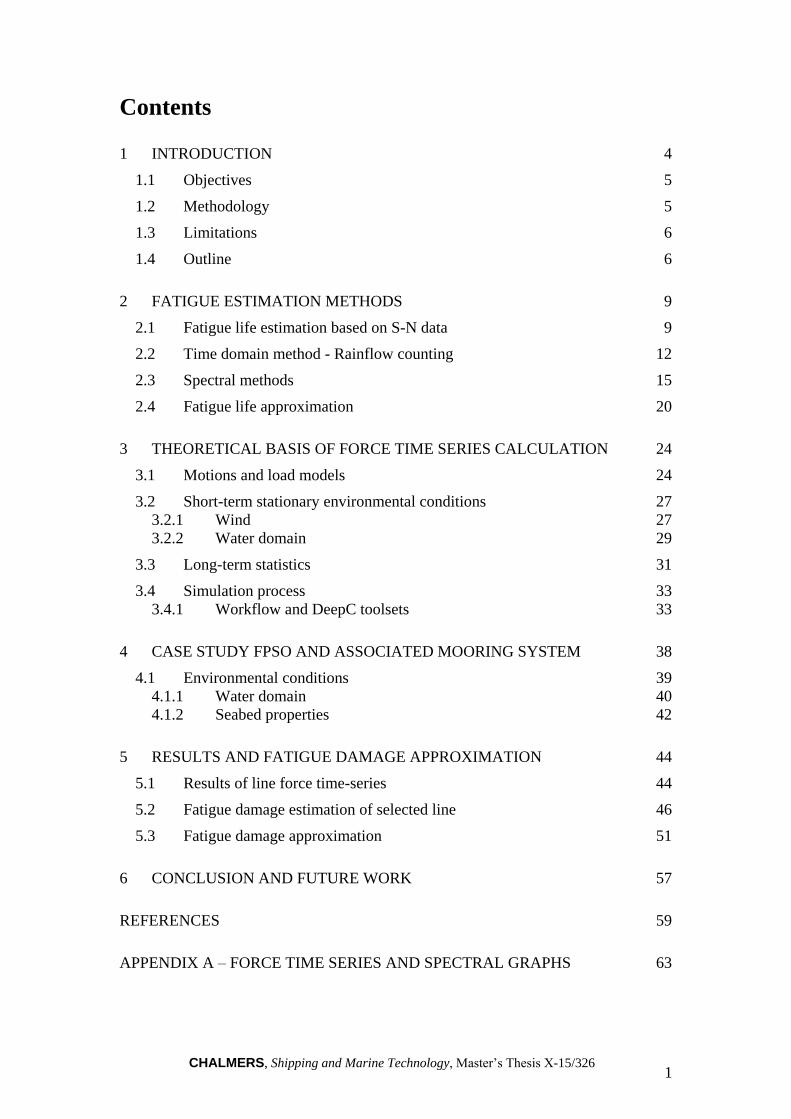
Contents
1 INTRODUCTION 4
1.1 Objectives 5
1.2 Methodology 5
1.3 Limitations 6
1.4 Outline 6
2 FATIGUE ESTIMATION METHODS 9
2.1 Fatigue life estimation based on S-N data 9
2.2 Time domain method - Rainflow counting 12
2.3 Spectral methods 15
2.4 Fatigue life approximation 20
3 THEORETICAL BASIS OF FORCE TIME SERIES CALCULATION 24
3.1 Motions and load models 24
3.2 Short-term stationary environmental conditions 27
3.2.1 Wind 27
3.2.2 Water domain 29
3.3 Long-term statistics 31
3.4 Simulation process 33
3.4.1 Workflow and DeepC toolsets 33
4 CASE STUDY FPSO AND ASSOCIATED MOORING SYSTEM 38
4.1 Environmental conditions 39
4.1.1 Water domain 40
4.1.2 Seabed properties 42
5 RESULTS AND FATIGUE DAMAGE APPROXIMATION 44
5.1 Results of line force time-series 44
5.2 Fatigue damage estimation of selected line 46
5.3 Fatigue damage approximation 51
6 CONCLUSION AND FUTURE WORK 57
REFERENCES 59
APPENDIX A – FORCE TIME SERIES AND SPECTRAL GRAPHS 63

CHALMERS, Shipping and Marine Technology, Master’s Thesis X-15/326 2
Preface
This thesis is part of the requirements for the master’s degree in Naval Architecture and
Ocean Engineering at Chalmers University of Technology, Göteborg, and has been
carried out at the Division of Marine Design, Department of Shipping and Marine
Technology, Chalmers University of Technology between January 2015 and June of
2015.
Above all I would like to thank my supervisor and examiner, Associate professor
Wengang Mao at Department of Shipping and Marine Technology, for not only he was
kind enough to propose a project in a framework of my preference, but showed much
more concern and spent more time than expected. Furthermore I should show gratitude
to Professor Igor Rychlik of the Department of Mathematical Sciences for his support
during this thesis project.
I may as well thank the Department for providing the resources needed to complete this
project and supporting me in any way possible.
Rioshar Yarveisy
May, 2015

CHALMERS, Shipping and Marine Technology, Master’s Thesis X-15/326 3
CHALMERS, Shipping and Marine Technology, Master’s Thesis X-15/326 4
1 Introduction
In a study by the National Institute of Standards and Technology, a division in U.S.
department of commerce, in 1983 with the subject of domestic economic effects of
fracture of materials, where the term “fracture” held a broader meaning than the
technical aspect, including deformation related problems as delamination in addition to
cracking. These estimates included not only the physical costs but the man power and
design efforts caused by these matters. The results showed 119 billion U.S. dollars in
1982, equal to 4% of the GNP (Gross National Product). Separate studies estimated a
total of 10% of GNP in case the damages from corrosion and wear have been included
in the results. A similar study of the fracture costs in Europe showed reported the same
4% of the GNP. This similarity can be utilized to conclude the same amounts apply to
all industrialized nations. The mentioned economic impact illustrates the importance of
accurate and reliable fatigue analysis methods (Milne, 1994).
According to Dowling (2013), “A deformation failure is a change in physical
dimensions or shape of a component that is sufficient for its function to be lost or
impaired”. This so called deformation failure can be caused by time dependent
elastic/plastic or time independent creep deformations, fracture due to static loading
including brittle, ductile, environmental and creep rupture might also be the cause. But
in the present work we are merely interested in fracture due to fatigue in cyclic loading.
All components in a mechanical system undergo repeated loading. These repeated loads
or cyclic loads cause varying stresses on the said components, these stresses may as
well be far below the material’s ultimate or yield strength. Although small, these cyclic
loads cause microscopic damage to material structure and during time may accumulate
with same loading patterns, develop into cracks or other forms of microscopic damage
and, if time is given, cause failure. This process of damage initiation to failure due to
cyclic loading is known as the fatigue process.
Although there where publications considering fatigue by late 1830s the matter did not
receive much attention until the famous Versailles train crash of 1842, where Rankine
recognized fatigue failure of axle as the incident cause (Rankine, 1842). Although the
theoretical groundwork for fatigue analysis was developed by 1950s many other cases
have pushed the research towards better understanding of fatigue and different modes
of failure throughout the coming and preceding years, as the Liberty ships of the WWII
where 30% of the 2700 vessels built from 1942 till the end of war suffered catastrophic
fracture such as SS Schenectady T2 tanker which broke in half with no warning. The
cause was later recognized as brittle fracture and no human fault was reported. This was
due to general technological unawareness of fracture mechanic principals (Wright,
2005). Another case worthy to mention is De Havilland DH 106 Comet, the first
production commercial jetliner, many of which suffered from problems, including two
plane crashes. The cause was later introduced as skin fatigue cracks at the corner of
windows due to stress concentration in sharp window corners (Atkinson, 1960). And
just to name a few more the Hawaiian airline Boeing incident, or the Eschede train
disaster.
Based on guidelines provided in position mooring offshore standards (DNV, 2013) a
fatigue limit state study is required for all long term moored units. Long term mooring
is defined as being positioned at the same location for more than five years. This process
includes a presentation of long term environment in terms of directions and different
sea state. The number of required sea states varies from 10 to 50 sea states although
fatigue damage might be sensitive to the number of sea states which calls for a

CHALMERS, Shipping and Marine Technology, Master’s Thesis X-15/326 5
sensitivity study of fatigue life regarding this issue. While necessary, this approach
imposes extra costs in terms of manpower on the manufacturer and end user of the
related product. The matter of capital investment and market competition asks for more
reliable and accurate structural analysis toolsets and applicable methods so that the costs
of production become the least possible.
The present thesis work puts the effort on studying and comparing different fatigue life
estimation approaches in addition to introducing fatigue life approximation
methodology based on Wiener Chaos expansion and Gauss approximation formula to
reduce the effort obtaining data regarding this matter.
1.1 Objectives
To calculate the fatigue life of given mooring equipment one normally refers to the
provided S-N curves including the mandatory safety factors by the regulatory body of
choice using either direct rainflow counting or spectral methods to acquire stress ranges.
The stresses are the product of time or frequency domain analysis of the system. To
reduce the effort put on simulations one might choose to implement fatigue life
approximation methods. The most common approach is utilizing the Gauss propagation
formula, another promising method can be the Wiener Chaos expansion (Sarkar, 2011).
Here the objective is to implement the two methods on fatigue results obtained from a
time domain dynamic simulation to evaluate and compare the two approaches and their
level of accuracy.
The aim of this thesis work can be summarized as follows:
An introduction to common fatigue assessment methods
Provide an insight to methods of fatigue approximation
Define the steps and methodology used in time domain dynamic analysis and
define the parameters involved
Provide an insight to the simulation process and motivate the choices made
Estimate the fatigue damage of loads using direct rainflow counting and
introduced spectral methods
Compare and evaluate the results from Wiener chaos expansion and Gauss
approximation against estimated fatigue damages
1.2 Methodology
Fatigue damage assessment in a station keeping operation is achieved through
calculation of loads on mooring components. These loads are results of hydrodynamic
loading of a vessel due to environmental conditions, hydrostatic loads, line mass related
inertia and weight forces and forced motions due to vessel position. By obtaining these
loads through frequency or more advanced time domain simulations one can assess the
fatigue damage through identifying load cycles by direct or spectral methods and
implementing the so called S-N curves. Another step forward can be evaluation of
methods to approximate the fatigue damage not limited to number of simulations and
based on parameters of choice.
In this assessment and based on the above requirements the first step is to acquire
detailed hydrodynamic and hydrostatic characteristics of the floating body, then by
providing environmental data and simulating the desired conditions one obtains vessel
motions and through transfer functions, loads at the mooring lines. Afterwards, by
implementing fatigue damage estimation approaches one can evaluate the fatigue

CHALMERS, Shipping and Marine Technology, Master’s Thesis X-15/326 6
damage intensity of the studied component, based on direct rainflow counting and or
spectral methods. Then the short term results will be used to approximate the long term
expected fatigue damage utilizing Wiener chaos expansion or Gaussian approximation
for stochastic estimation of the fatigue life. The methodology in terms of steps and
approaches implemented in this study is illustrated in Figure 1-1.
Figure 1-1 An overview of simulation, fatigue methodology and approximation methods and the
steps to achieve results
1.3 Limitations
For the present thesis work the hull, hydrodynamic and hydrostatic characteristics of
the vessel used in simulations is the model provided by the software package. The fact
the simulation parameters and conditions used to obtain the vessel characteristics are
unknown can considered to be a limiting factor. On the other hand as the site specific
metocean data is not available all the input parameters are presumptuous and limited to
provided statistical data and approaches recommended through class guidelines (DNV,
2014a). Although these conditions do not have much effect on the aim of this project
the input conditions might as well cause some inconsistencies between reality and the
simulated cases. In the following chapters the theoretical aspect of the statistical
approach will be defined in detail. But as a limitation and a peek into the future work
in order to utilize the Hermite polynomial expansion it is assumed that the damage rate
is a function of independent normal variables. For the sake of simplicity here a one
dimensional dependency of damage is studied and the standard normal variable here is
chosen to be representative of Hs, the specific wave height. Furthermore and as will be
referred to, based on DNV guidelines (DNV, 2014a) the specific wave heights best fit
to Weibull distribution. This transformation of data from normal to Weibull
distribution, where we obtain the environmental conditions, gives sea states with
specific wave heights and peak periods with accuracies, which the software might not
be able to count for.
1.4 Outline
Following the overview of methodology in Figure 1-1 the present work can be divided
into three parts, part one defining the environmental conditions and model to go through
the simulation process of software, then implementing fatigue assessment methods to
obtain fatigue damage of selected line component and finally fatigue damage
approximation using Wiener chaos expansion and Gaussian propagation to compare the
results with the estimated fatigue damage.
To do so we start with an introduction to fatigue estimation and approximation methods
in chapter 2, provide an insight to the simulation process and theoretical aspect of the

CHALMERS, Shipping and Marine Technology, Master’s Thesis X-15/326 7
software including implemented approaches to procure the environmental conditions as
input in chapter 3. Chapter four includes an insight to the theoretical structure of the
case study FPSO and the applied environmental conditions. After this and obtaining
results of line tensions we then move on to assessing the fatigue damage and
comparison of two implemented methods of direct rainflow counting and various
methods of spectral analysis in chapter five. In addition the two mentioned damage
approximation schemes are applied and the results are evaluated against the fatigue
assessment methods in the same chapter.

CHALMERS, Shipping and Marine Technology, Master’s Thesis X-15/326 8

CHALMERS, Shipping and Marine Technology, Master’s Thesis X-15/326 9
2 Fatigue estimation methods
By now there are three methods to evaluate and design against fatigue damage. The
stress based approach developed to its current form by mid-fifties, where the basis lies
on the nominal stresses across the cross section of the component. The result of this
approach is the nominal stress which the designed component can resist, by adjusting
the nominal stress of the standard specimen to the stress risers or notches of the
component. Another method providing more detailed local yielding analysis of the
component is the strain based approach. The last available method is the fracture
mechanics approach where the crack growth is studied through its initiation to failure
utilizing the laws of fracture mechanics (Dowling, 2013).
Considering two cyclic loading fatigue modes of high cycle and low cycle fatigue,
elastic and plastic deformations are dominant in the same respect. DNV-RP-C203
(DNV, 2011) describes low cycle and high cycle fatigue as: “By fatigue strength
assessment of offshore structure is normally understood capacity due to high cycle
fatigue loading. By high cycle loading is normally understood cycles more than 10 000.
For example stress response from wave action shows typically 5 million cycles a year.
A fatigue assessment of response that is associated with number of cycles less than 10
000 is denoted low cycle fatigue”. Low cycle fatigue is characterized by creation of
local regions with plastic behavior, and as strains are the more measurable parameter
they become the dominant factor in the analysis, on the other hand and in case of high
cycle fatigue due to elastic deformations measuring stresses becomes the main means
of analysis. As the scope of this master’s thesis focuses on high cycle fatigue the effort
is put on to provide a more detailed insight into the subject. In this chapter an overview
of the high-cycle (stress based) fatigue methodology on fatigue life calculation, using
S-N curves after implementing direct rainflow counting or spectral methods is
presented. Considering the aim of this thesis it seemed fit to mention definition and
explanation of the two fatigue approximation methods, Wiener chaos expansion and
Gauss propagation here as well.
2.1 Fatigue life estimation based on S-N data
In high cycle fatigue problem of offshore structures, one often employs S-N curve and
linear Palmgren-Miner law for the fatigue life prediction. The S-N curves are obtained
through multiple fatigue tests executed at different stress levels, where considerable
statistical scatter in the fatigue life will be observed (Dowling, 2013). The deviation of
fatigue life in spite of similarity in test specimen and loading conditions is due to
sample-to-sample material differences, microscopic defects, surface roughness as well
as human errors such as specimen alignment. The fatigue life versus stress amplitude is
illustrated in Figure 2-1.
Figure 2-1 Example of fatigue life to failure data scatter in rotating bending test (Dowling, 2013).

CHALMERS, Shipping and Marine Technology, Master’s Thesis X-15/326 10
If the data scatter relating fatigue life to stress amplitude is studied, usually the result
will be a skewed distribution. However logarithm of 𝑁𝑓 , fatigue life, represents a
standard normal variable as in Figure 2-2 (Dowling, 2013).
Figure 2-2 Distribution of fatigue life for 57 small specimens of 7075-T6 aluminium. Left the
skewed distribution right standard normal distribution of 𝐥𝐨𝐠(𝑵𝒇) (Dowling, 2013)
There also exists use of other statistical distributions such as the Weibull distribution.
The statistical analysis of 𝑁𝑓helps develop the average S-N curves and complementing
S-N curves for different possibilities of failure. The provided S-N curves in DNV-RP-
C203 (DNV, 2011) are representing life expectation versus stress range based on mean
value minus twice the standard deviation of the experimental data. This implies the
probability of failure non-occurrence of 97.7%.
In order to calculate the fatigue life of the specimen based on the S-N curve one utilizes
a logarithmic function as follows:
log(𝑁𝑡) = log(�̅�) − 𝑚𝑙𝑜𝑔(∆𝑆) (1)
Where:
𝑁𝑡 Being the number of cycles to failure
∆𝑆 The stress range
𝑚 Slope of the S-N curve
�̅� The intercept of the S-N curve
The S-N curves provided by DNV-OS-E301 (DNV, 2013), valid for stud and studless
chains, stranded and spiral wire ropes used to estimate fatigue life of the mooring chains
in the present thesis are shown in Figure 2-3. Where the curve slope and intercepts are
as stated in Table 2-1.
Table 2-1 Curve slope and intercept constants of the S-N curves in Figure 2-3
�̅� 𝒎
Stud chain 𝟏. 𝟐𝑬𝟏𝟏 𝟑. 𝟎
Studless chain 𝟔. 𝟎𝑬𝟏𝟎 𝟑. 𝟎
Stranded rope 𝟑. 𝟒𝑬𝟏𝟒 𝟒. 𝟎
Spiral rope 𝟏. 𝟕𝑬𝟏𝟕 𝟒. 𝟎

CHALMERS, Shipping and Marine Technology, Master’s Thesis X-15/326 11
Figure 2-3 Design S-N curve for mooring chains and wire ropes (DNV, 2013)
It should be noted that the S-N curves above are only applicable to tension-tension
cyclic loading. In the provided S-N curves by the DNV rules and regulations the effect
of steel grade is not accounted for and the only factor is the geometry of the mooring
lines.
In practical matters, cyclic loading of mechanical components is normally highly
irregular, i.e. variable amplitude load conditions. To estimate the fatigue life of
components undergoing such load histories the vastly used Palmgren–Miner rule is
introduced here. Consider irregular variable amplitude loading time history, as
presented in Figure 2-4 similar to this case in all stress time histories, certain counting
algorithm should be applied for getting a number of cycles from the loading history.
The corresponding damage for one cycle of such stress amplitude will be found from
the S-N curves. The Palmgren-Miner rule utilizes the available data to calculate the life
to failure as formulated in equation (2).
Figure 2-4 Left an irregular variable amplitude load time history and right, S-N curve used to
obtain the fatigue life in respect to stress amplitude of individual cycles (Dowling, 2013).
The Palmgren-Miner rule states that for a given stress-time history cycles, the induced
fatigue damage can be computed using a chosen S-N curve as follows:
CHALMERS, Shipping and Marine Technology, Master’s Thesis X-15/326 12
𝐷𝑡𝑜𝑡 = ∑
𝑁𝐽
𝑁𝐹𝑗
𝑘
𝑗=1
=1
�̅�∑ 𝑁𝐽
𝑘
𝑗=1
(∆𝜎)𝑚 (2)
Where:
𝑁𝐽 Number of cycles with same stress range
𝑁𝐹𝑗 Number of cycles to failure for a specific stress range
𝑘 Number of cycles with different stress ranges
�̅� Intercept of the S-N curve
𝑚 Slope of the S-N curve
∆𝑆 Stress range of amplitude based on the input data needed for S-N curve
𝐷𝑡𝑜𝑡 Total accumulated damage during the stress time history
In principle, fatigue failure occurs when the total damage Dtot is larger or equals to 1,
this means that 100% of the life is exhausted.
2.2 Time domain method - Rainflow counting
In order to obtain the fatigue life of a component, one may use the adjusted stress
amplitude of the component in respect to stress concentration factors of a notched
member from an S-N curve of the said material. Usually the extraction of data points
used in regression analysis of forming an S-N curve involves a scheme named constant
amplitude stressing. In constant amplitude testing the specimen goes through cycling
between constant maximum and minimum stress levels. The difference of maximum
and minimum stresses is the stress range and half this magnitude is called stress
amplitude. The random stress variations of real world practices are recorded and
presented in the same manner. To utilise the available S-N curves one should be able to
identify the stress range and mean of individual cycles. This can be managed by one of
the available rainflow counting methods or spectral approaches. When facing highly
irregular load histories with time the order in which how individual events should be
considered as a cycle or otherwise is not clear so that the Palmgren miner rule can be
employed.
The stress cycles are counted from the local maxima (peaks) and minima (troughs) of
the stress history by some cycle counting method.
The simplest counting method is the so-called min-Max (Max-min) counting method,
where the local maximum is paired with the preceding local minimum. The stress cycles
in this method only consider the effect of local stresses, but ignore the global effect
including large cycles. Therefore, this method is not capable of estimating the risk of
fatigue failure, since it gives non-conservative (too small) fatigue damages.
The most frequently used rainflow counting method is developed on the hysteretic
properties of material, where the cyclic stress-strain curves form hysteretic loops. The
local maxima are represented by tops of the loops, while local minima by bottoms of
the loops. The rainflow method is to identify the local minimum which should be paired
with a local maximum to form a hysteretic loop. It is believed to give the most
“accurate” fatigue life predictions (Dowling, 2013).
CHALMERS, Shipping and Marine Technology, Master’s Thesis X-15/326 13
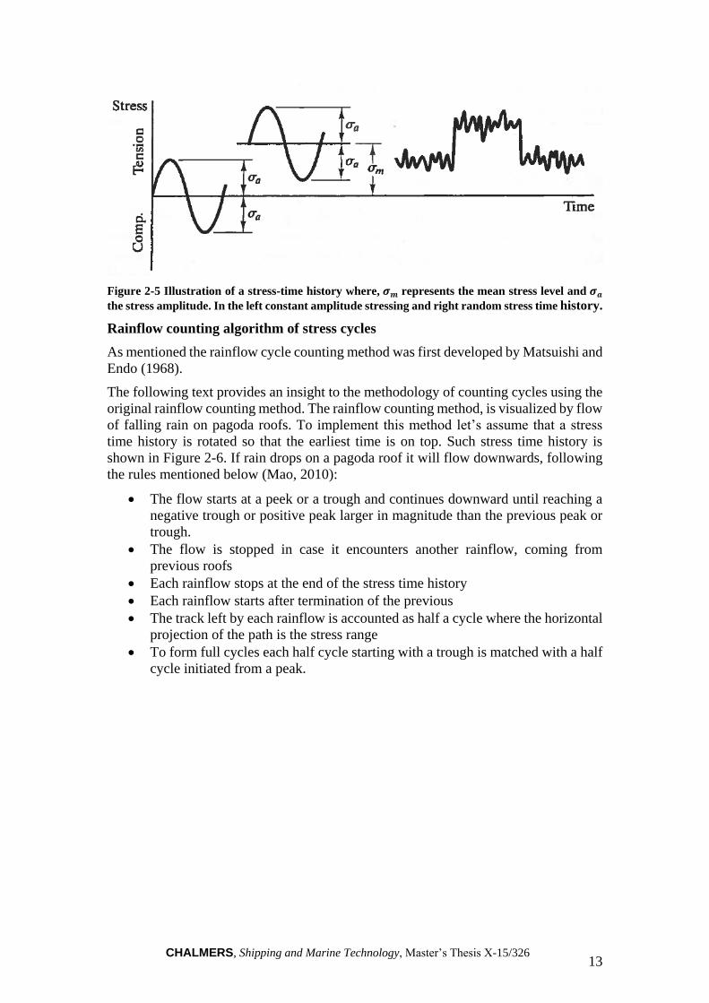
Figure 2-5 Illustration of a stress-time history where, 𝝈𝒎 represents the mean stress level and 𝝈𝒂
the stress amplitude. In the left constant amplitude stressing and right random stress time history.
Rainflow counting algorithm of stress cycles
As mentioned the rainflow cycle counting method was first developed by Matsuishi and
Endo (1968).
The following text provides an insight to the methodology of counting cycles using the
original rainflow counting method. The rainflow counting method, is visualized by flow
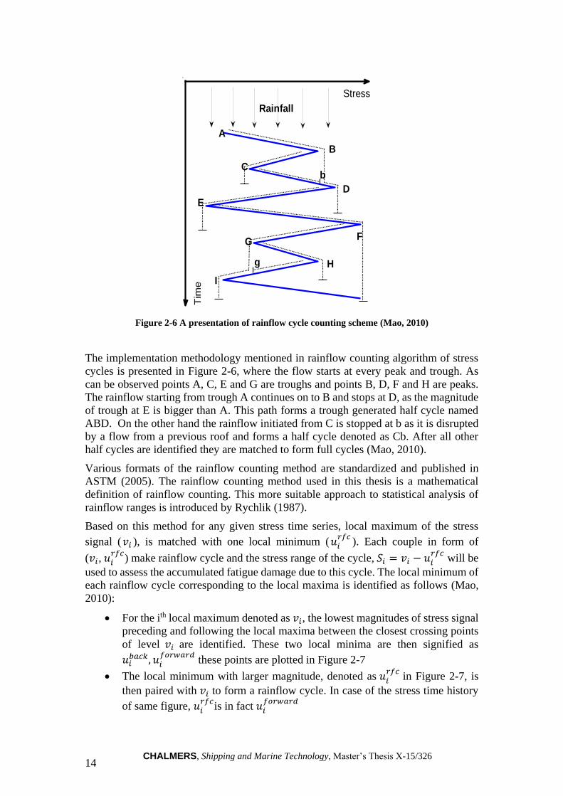
of falling rain on pagoda roofs. To implement this method let’s assume that a stress
time history is rotated so that the earliest time is on top. Such stress time history is
shown in Figure 2-6. If rain drops on a pagoda roof it will flow downwards, following
the rules mentioned below (Mao, 2010):
The flow starts at a peek or a trough and continues downward until reaching a
negative trough or positive peak larger in magnitude than the previous peak or
trough.
The flow is stopped in case it encounters another rainflow, coming from
previous roofs
Each rainflow stops at the end of the stress time history
Each rainflow starts after termination of the previous
The track left by each rainflow is accounted as half a cycle where the horizontal
projection of the path is the stress range
To form full cycles each half cycle starting with a trough is matched with a half
cycle initiated from a peak.
CHALMERS, Shipping and Marine Technology, Master’s Thesis X-15/326 14
Figure 2-6 A presentation of rainflow cycle counting scheme (Mao, 2010)
The implementation methodology mentioned in rainflow counting algorithm of stress
cycles is presented in Figure 2-6, where the flow starts at every peak and trough. As
can be observed points A, C, E and G are troughs and points B, D, F and H are peaks.
The rainflow starting from trough A continues on to B and stops at D, as the magnitude
of trough at E is bigger than A. This path forms a trough generated half cycle named
ABD. On the other hand the rainflow initiated from C is stopped at b as it is disrupted
by a flow from a previous roof and forms a half cycle denoted as Cb. After all other
half cycles are identified they are matched to form full cycles (Mao, 2010).
Various formats of the rainflow counting method are standardized and published in
ASTM (2005). The rainflow counting method used in this thesis is a mathematical
definition of rainflow counting. This more suitable approach to statistical analysis of
rainflow ranges is introduced by Rychlik (1987).
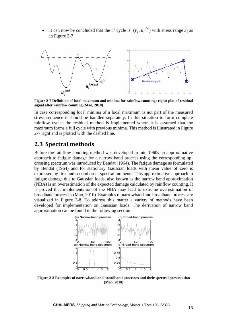
Based on this method for any given stress time series, local maximum of the stress
signal (𝑣𝑖 ), is matched with one local minimum (𝑢𝑖𝑟𝑓𝑐
). Each couple in form of
(𝑣𝑖, 𝑢𝑖𝑟𝑓𝑐
) make rainflow cycle and the stress range of the cycle, 𝑆𝑖 = 𝑣𝑖 − 𝑢𝑖𝑟𝑓𝑐
will be
used to assess the accumulated fatigue damage due to this cycle. The local minimum of
each rainflow cycle corresponding to the local maxima is identified as follows (Mao,
2010):
For the ith local maximum denoted as 𝑣𝑖, the lowest magnitudes of stress signal
preceding and following the local maxima between the closest crossing points
of level 𝑣𝑖 are identified. These two local minima are then signified as
𝑢𝑖𝑏𝑎𝑐𝑘, 𝑢𝑖
𝑓𝑜𝑟𝑤𝑎𝑟𝑑 these points are plotted in Figure 2-7
The local minimum with larger magnitude, denoted as 𝑢𝑖𝑟𝑓𝑐
in Figure 2-7, is
then paired with 𝑣𝑖 to form a rainflow cycle. In case of the stress time history
of same figure, 𝑢𝑖𝑟𝑓𝑐
is in fact 𝑢𝑖𝑓𝑜𝑟𝑤𝑎𝑟𝑑
-6 170
13
Stress
Tim
e
A
Cb
D
E
FG
Hg
I
B
Rainfall
CHALMERS, Shipping and Marine Technology, Master’s Thesis X-15/326 15
It can now be concluded that the ith cycle is (𝑣𝑖, 𝑢𝑖𝑟𝑓𝑐
) with stress range 𝑆𝑖 as
in Figure 2-7
Figure 2-7 Definition of local maximum and minima for rainflow counting; right: plot of residual
signal after rainflow counting (Mao, 2010)
In case corresponding local minima of a local maximum is not part of the measured
stress sequence it should be handled separately. In this situation to form complete
rainflow cycles the residual method is implemented where it is assumed that the
maximum forms a full cycle with previous minima. This method is illustrated in Figure
2-7 right and is plotted with the dashed line.
2.3 Spectral methods
Before the rainflow counting method was developed in mid 1960s an approximative
approach to fatigue damage for a narrow band process using the corresponding up-
crossing spectrum was introduced by Bendat (1964). The fatigue damage as formulated
by Bendat (1964) and for stationary Gaussian loads with mean value of zero is
expressed by first and second order spectral moments. This approximative approach to
fatigue damage due to Gaussian loads, also known as the narrow band approximation
(NBA) is an overestimation of the expected damage calculated by rainflow counting. It
is proved that implementation of the NBA may lead to extreme overestimation of
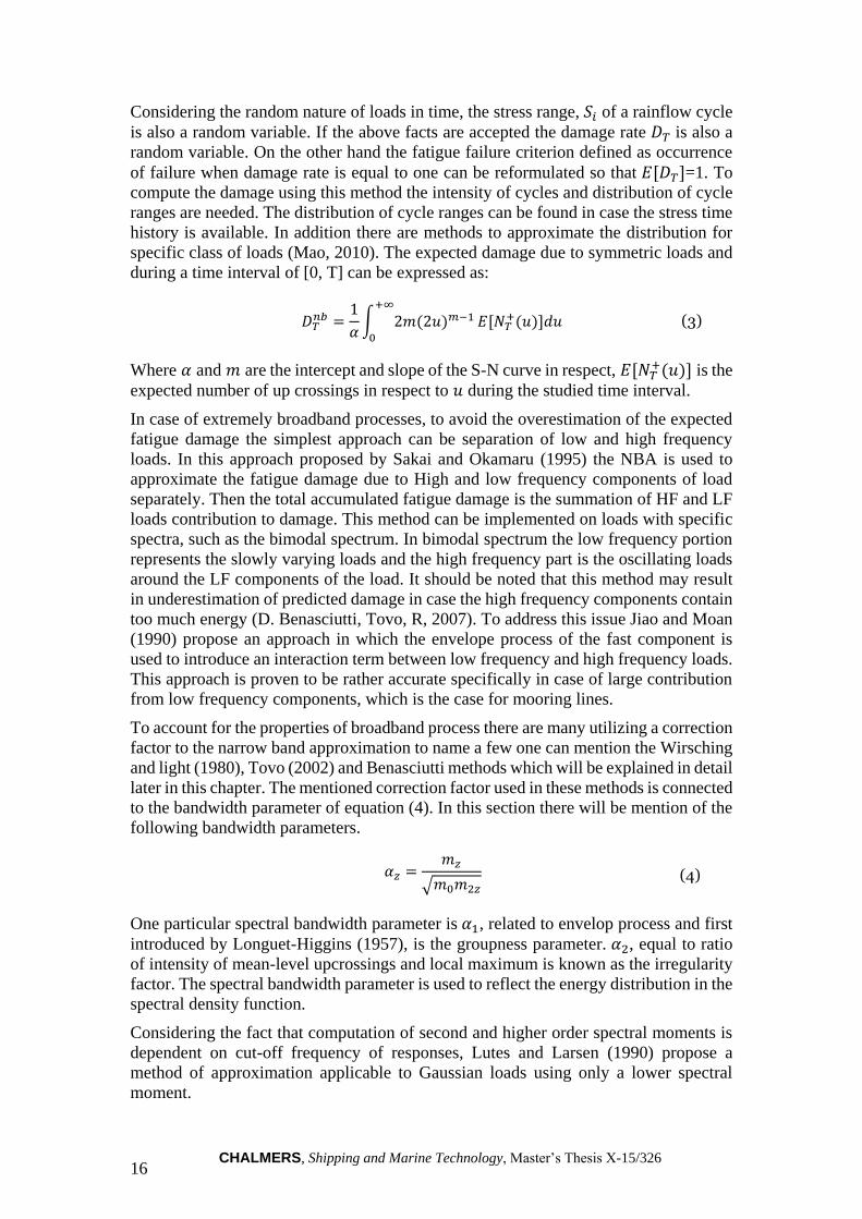
broadband processes (Mao, 2010). Examples of narrowband and broadband process are
visualized in Figure 2-8. To address this matter a variety of methods have been
developed for implementation on Gaussian loads. The derivation of narrow band
approximation can be found in the following section.
Figure 2-8 Examples of narrowband and broadband processes and their spectral presentation
(Mao, 2010)
0 2 4 6 8 10 12 14 16 18 20-5
0
5
10
15
Residual signal
CHALMERS, Shipping and Marine Technology, Master’s Thesis X-15/326 16
Considering the random nature of loads in time, the stress range, 𝑆𝑖 of a rainflow cycle
is also a random variable. If the above facts are accepted the damage rate 𝐷𝑇 is also a
random variable. On the other hand the fatigue failure criterion defined as occurrence
of failure when damage rate is equal to one can be reformulated so that 𝐸[𝐷𝑇]=1. To
compute the damage using this method the intensity of cycles and distribution of cycle
ranges are needed. The distribution of cycle ranges can be found in case the stress time
history is available. In addition there are methods to approximate the distribution for
specific class of loads (Mao, 2010). The expected damage due to symmetric loads and
during a time interval of [0, T] can be expressed as:
𝐷𝑇
𝑛𝑏 =1
𝛼∫ 2𝑚(2𝑢)𝑚−1
+∞
0
𝐸[𝑁𝑇+(𝑢)]𝑑𝑢 (3)
Where 𝛼 and 𝑚 are the intercept and slope of the S-N curve in respect, 𝐸[𝑁𝑇+(𝑢)] is the
expected number of up crossings in respect to 𝑢 during the studied time interval.
In case of extremely broadband processes, to avoid the overestimation of the expected
fatigue damage the simplest approach can be separation of low and high frequency
loads. In this approach proposed by Sakai and Okamaru (1995) the NBA is used to
approximate the fatigue damage due to High and low frequency components of load
separately. Then the total accumulated fatigue damage is the summation of HF and LF
loads contribution to damage. This method can be implemented on loads with specific
spectra, such as the bimodal spectrum. In bimodal spectrum the low frequency portion
represents the slowly varying loads and the high frequency part is the oscillating loads
around the LF components of the load. It should be noted that this method may result
in underestimation of predicted damage in case the high frequency components contain
too much energy (D. Benasciutti, Tovo, R, 2007). To address this issue Jiao and Moan
(1990) propose an approach in which the envelope process of the fast component is
used to introduce an interaction term between low frequency and high frequency loads.
This approach is proven to be rather accurate specifically in case of large contribution
from low frequency components, which is the case for mooring lines.
To account for the properties of broadband process there are many utilizing a correction
factor to the narrow band approximation to name a few one can mention the Wirsching
and light (1980), Tovo (2002) and Benasciutti methods which will be explained in detail
later in this chapter. The mentioned correction factor used in these methods is connected
to the bandwidth parameter of equation (4). In this section there will be mention of the
following bandwidth parameters.
𝛼𝑧 =𝑚𝑧
√𝑚0𝑚2𝑧
(4)
One particular spectral bandwidth parameter is 𝛼1, related to envelop process and first
introduced by Longuet-Higgins (1957), is the groupness parameter. 𝛼2, equal to ratio
of intensity of mean-level upcrossings and local maximum is known as the irregularity
factor. The spectral bandwidth parameter is used to reflect the energy distribution in the
spectral density function.
Considering the fact that computation of second and higher order spectral moments is
dependent on cut-off frequency of responses, Lutes and Larsen (1990) propose a
method of approximation applicable to Gaussian loads using only a lower spectral
moment.

CHALMERS, Shipping and Marine Technology, Master’s Thesis X-15/326 17
Considering the fact that Gaussian loads in real world applications are rare, the spectral
presentation of loads alone is not sufficient enough to define the cumulative distribution
function of the loads. To solve this problem if statistical characteristics of the load
history, skewness and kurtosis, are known the load history can be transferred to a
Gaussian distribution (Mao, 2010).
Implemented spectral approaches
In this study eight spectral approaches to fatigue damage intensity are implemented for
later comparison with the approximative WCE and Gaussian methods. Here the aim is
to provide a basic definition of these methods.
For a stationary process the power spectral density 𝑆(𝜆), is defined by the spectral
moments of the process.
𝑚𝑧 = ∫ 𝜆𝑧𝑆(𝜆)
∞
0
𝑑𝜆 (5)
Following the above equation 𝑚0 = 𝑉[𝑊(𝑡)] and 𝑚2 = 𝑉[𝑊′(𝑡)] where V is the
variance and W a continuous load process (Bengtsson, 2009). The spectral moments of
a degenerated case is formulated as 𝑚𝑧 = 𝜆𝑝𝑧 𝜎2 in case the spectrum contains only one
frequency (𝛾𝑝 = 2𝜋 𝑇𝑝⁄ ). In this specific case the load process is expressed as follows:
𝑊(𝑡) = 𝜎𝑅𝑐𝑜𝑠(2𝜋 𝑇𝑝 + 𝜙⁄ ) (6)
Where R is a standard distributed Rayleigh random variable (Rayleigh, 1880) and
independent of the phase 𝜙. Other than the aforementioned bandwidth parameter there
is also mention of the generalized average period in literature where:
𝑇𝑧 = 2𝜋(𝑚0 𝑚𝑧⁄ )1 𝑧⁄ (7)
In case 𝑧 = 2, 𝑇2 is defined as the mean period.
The spectral approaches implemented in the scope of this thesis work are fatigue
damage intensity approximation schemes. The explicit formula of fatigue damage
intensity for the case of constant amplitude loading, where the load process W is defined
in equation (6), can be computed as:
𝑑(𝑘) =
𝑚0𝑘 2⁄
𝑇𝑝23𝑘 2⁄ Γ(1 + 𝑘 2⁄ ) (8)
Where k is the slope of the applicable S-N curve.
We first start with the case of a cosine load process with Tp as its peak period. In this
condition, for any 𝑧 ≥ 0 the peak period and zero up crossing period are equal (𝑇𝑝 =
𝑇𝑧). Considering the formula of damage intensity in equation (8) and the equality of
peak period and zero up crossing period in case of a cosine load history the damage can
be formulated as in equation (9).
𝑑(𝑘) =
𝑚0𝑘 2⁄
𝑇𝑧23𝑘 2⁄ Γ(1 + 𝑘 2⁄ ) (9)
CHALMERS, Shipping and Marine Technology, Master’s Thesis X-15/326 18
Following the above equations the damage intensity for a non-degenerated spectrum
𝑆(𝜆) can be estimated by equation (10).
𝑑𝑧(𝑘) =
𝑚0𝑘 2⁄
𝑇𝑧23𝑘 2⁄ Γ(1 + 𝑘 2⁄ ) (10)
Considering the fact that 𝑑2(1) = 𝑑(1) from equations (9) and (10) and 𝑑2(𝑘) ≥ 𝑑(𝑘),
defining 𝑑2(𝑘) as the upper bound of damage rainflow damage (Rychlik, 1993) it can
be concluded that it is the sharpest bound of damage. Damage approximation using
𝑑𝑧(𝑘) method with 𝑧 < 2 is an approach to provide non-conservative assessment of
damage for low values of k and reduce the conservativeness of the method for cases
with large k values (Bengtsson, 2009).
As mentioned in the previous section due to dependence of the 2nd and higher order
spectral moments on the cut-off frequency Lutes and Larsen propose a simple
approximation method. Where z is a varying parameter dependant on k (𝑧 = 2 𝑘⁄ ). The
proposed single approximation is formulated as in equation (11).
𝑑𝐿𝐿(𝑘) =
𝑚0𝑘 2⁄
𝑇2 𝑘⁄23𝑘 2⁄ Γ(1 + 𝑘 2⁄ ) =
𝑚2 𝑘⁄𝑘 2⁄
2𝜋23𝑘 2⁄ Γ(1 + 𝑘 2⁄ ) (11)
From the above equation it can be concluded that for 𝑘 ≥ 2, 𝑑2
𝑘
(𝑘) ≤ 𝑑1(𝑘).
The spectral bandwidth parameters 𝛼𝑧 can reduce the conservativeness of damage
intensity calculated by the upper bound 𝑑2(𝑘) considering the fact that 𝛼𝑧 < 1. Many
approximation methods use this approach to provide more realistic results. One of
which is proposed by Tovo (2002). Where it is proposed to approximate damage using
equation (12).
𝑑𝐵𝑇(𝑘) = (𝑝 + (1 − 𝑝)𝛼2𝑘−1)𝑑2(𝑘) (12)
In literature it is proposed to use 𝑝 = min (𝛼1−𝛼2
1−𝛼1, 1) where using p=1 makes the
expected damage to be equal to the upper bound 𝑑2(𝑘). Benasciutti (2004) proposes an
improvement to the approximation implementing a new formulation for p as presented
in equation (13).
𝑝 = (𝛼
1− 𝛼2)
1.112𝑒2.11𝛼2(1 − 𝛼1 − 𝛼2 + 𝛼1𝛼2) + (𝛼1 − 𝛼2)
(𝛼2 − 1)2 (13)
Wirsching and Light (1980) propose a method where fatigue damage is approximate by
equation (14).
𝑑𝑊𝐿(𝑘) = (𝑎(𝑘) + (1 − 𝑎(𝑘)) (1 − √1 − 𝛼2
2)
𝑏(𝑘)
) 𝑑2(𝑘) (14)
Where parameters of the equation are:
𝑎(𝑘) = 0.926 − 0.033𝑘
𝑏(𝑘) = 1.587𝑘 − 2.323
CHALMERS, Shipping and Marine Technology, Master’s Thesis X-15/326 19
When implementing the narrow band approach there is a need for approximation of the
rainflow cycle range, h, and the damage intensity. The damage can be formulated as in
equation (15).
𝑑(𝑘) =
1
𝑇𝑚𝐸[ℎ𝑘|𝑘] (15)
Where the mean period 𝑇𝑚 can be calculated based on equation (16).
𝑇𝑚 = 2𝜋√
𝑚2
𝑚4 (16)
It is common assumption for the narrowband approximation to be defined with rainflow
range distribution of form 2√𝜆𝑅 distribution. In case the bandwidth parameter 𝛼2 is
converging to one R will be a Rayleigh distributed variable. From this one can calculate
the narrowband damage as (Bengtsson, 2009):
𝑑𝑛𝑏(𝑘) =
1
𝑇𝑚𝐸 [(2√𝑚0𝑅)
𝑘|𝑘] ≥ 𝑑4(𝑘) (17)
Considering the fact that in case of a constant k the damage intensity (𝑑𝑧(𝑘)) is an
increasing function of z and from Rychlik (1993) one can conclude that 𝑑4(𝑘) ≥𝑑2(𝑘) ≥ 𝑑(𝑘) which proves for this method to be even more conservative than the
expected damage approximated by 𝑑2(𝑘).
In a method proposed by Dirlik (1985) a less conservative approach in comparison with
narrowband approximation by using exponential and Rayleigh distributions is
introduced.
𝑑𝐷𝑖𝑟𝑙𝑖𝑘(𝑘) =𝑚0
𝑘2
𝑇𝑚(𝐷1𝑄𝑘Γ(1 + 𝑘) + (𝐷2|𝑅|𝑘 + 𝐷3) ∗ Γ(1 + 𝑘/2)2𝑘/2)
(18)
In equation (18) the terms 𝐷1, 𝐷2, 𝐷3, 𝑅 and 𝑄 are functions of 𝑚𝑖.
Zhao and Baker (1992) develop an approximation by fitting Weibull and Rayleigh
distributions to simulated rainflow ranges to find the relation of parameters and the
moments of the load process spectra.
𝑑𝑍𝐵(𝑘) = (1 − 𝑝)𝑑𝑛𝑏(𝑘) + 𝑝𝑚0
𝑘2
𝑇𝑚(8 − 7𝛼2)−𝑘/𝛽 ∗ 2𝑘Γ(1 + 𝑘/𝛽)
(19)
Where:
{𝛽 = 1.1 𝑓𝑜𝑟 𝛼2 > 0.9
𝛽 = 1.1 + 9(𝛼2−0.9) 𝑓𝑜𝑟 𝛼2 < 0.9
𝑝 =1−𝛼2
1−(8−7𝛼2)−
1𝛽Γ(1+1/𝛽)√2/𝜋
CHALMERS, Shipping and Marine Technology, Master’s Thesis X-15/326 20
2.4 Fatigue life approximation
To approximate the fatigue life of any specimen i.e. mooring chain independent of
simulation parameters e.g. specific wave height, two methods are introduced. The
Gaussian approximation formula and Wiener chaos expansion. Here the aim is to
describe the dependency of damage 𝑑(Θ) on parameters effecting the vector Θ. If Θ is
a function of standard normal variable 𝑍 = 𝑍1 … 𝑍𝑛 it can be said that Θ = Θ(𝑍) and
damage being a function of Θ we can say damage is a function of 𝑍. Although the
relation can be applied to any value of Θ = 𝜃 the Z is chosen to be a standard random
variable since the mean square error is minimal for a Gaussian Z. In the present case
for sake of simplicity we study 𝑍 as one dimensional.
Gaussian approximation
The Gaussian approach although rather accurate for small parameter variations and
requires less evaluation of the damage function is proven to be more sensitive in
comparison with Wiener chaos expansion. This can be problematic if the damage rate
is estimated based on the assumption of ergodicity of simulation result stresses. On the
other hand there exists uncertainties and hardship in numerical estimation of higher
order derivatives of the damage function. This might become an issue in case the local
curvature of the function is wrong and higher order Taylor terms are required. The
matter of higher order derivatives still applies in case higher accuracy is needed (Sarkar,
2011).
As said the most common approach to damage approximation for one dimensional 𝑍 is
the Gauss propagation formula:
𝑑(𝑍) ≈ 𝑑(0) +
𝜕𝑑
𝜕𝑍(0)𝑍 +
1
2
𝜕2𝑑
𝜕𝑍2(0)𝑍2 = 𝑑𝐺(𝑍) (20)
Where due to uncertainties of the second derivation the quadratic term is neglected.
Wiener chaos expansion
The other approach to approximate fatigue damage is the Wiener chaos method or the
method of Hermite polynomial chaos expansions. This method is utilized to solve a
wide variety of problems involving SPDEs (Stochastic Partial Differential Equations)
e.g. wave propagation and Navier-Stokes equations (Hou, 2006).
In the present thesis work the method is used to observe the dependency of fatigue
damage on specific wave height if two parameter Pierson-Moskowitz wave spectrum is
applied. In case the variance of the damage rate has a finite value (𝐸[𝑑(𝑍)2] < ∞),
then using the Hermite polynomial expansion is a valid approach. The formulation is
as follows:
𝑑(𝑍) = ∑ 𝑐𝑗𝐻𝑗(𝑍) ≈
∞
𝑗=0
∑ 𝑐𝑗𝐻𝑗(𝑍) =
𝑛
𝑗=0
𝑑𝑛(𝑍) (21)
Here 𝐻𝑗s are normalized Hermite polynomials:
𝐻0(𝑍) = 1, 𝐻1(𝑍) = 𝑍, 𝐻2(𝑍) = (𝑍2 − 1)/√2, 𝐻3(𝑍) = (𝑍3 − 3𝑍)/√6 ,
𝐻4(𝑍) = (𝑍4 − 6𝑍2 + 3)/√24
Where higher order polynomials can be calculated by:
CHALMERS, Shipping and Marine Technology, Master’s Thesis X-15/326 21
√𝑛 + 1𝐻𝑛−1(𝑍) = 𝑍𝐻𝑛(𝑍) − √𝑛𝐻𝑛−1(𝑥) (22)
And 𝑐𝑗 is:
𝑐𝑗 =
1
√2𝜋∫ 𝑑(𝑍)𝐻𝑗(𝑍)𝑒−𝑧2 2⁄ ≈
1
√2𝜋∑ ℎ𝑖𝑑(𝑧𝑖)𝐻𝑗(𝑧𝑖)𝑒−𝑧𝑖
2 2⁄
𝑛
𝑖=1
∞
−∞
(23)
In the above equation the terms (ℎ𝑖, 𝑧𝑖) are some quadrature scheme. Acting based on
the assumption that fatigue damage is a function of independent standard normal
variables, the specific wave height as the parameter of study and all other varying
environmental conditions should be chosen based on the selected normal variables. To
solve the integral and obtain value of cj for the random variables the Legendre-Gauss
quadrature integral approximation method with accuracy of n=20 is implemented. The
Legendre-Gauss Quadrature integral approximation for a single variable is defined as:
∫ 𝑓(𝑥)𝑑𝑥 = ∑ 𝑊𝑖𝑓(𝑥𝑖) = ∑ 𝑊𝑖𝑓(𝑥𝑖)
𝑛
𝑖=1
∞
𝑖=1
𝑏
𝑎
(24)
∫ 𝑓(𝑥)𝑑𝑥 =
𝑏 − 𝑎
2
𝑏
𝑎
∫ 𝑓(𝑏 − 𝑎
2𝑥𝑖 +
𝑏 + 𝑎
2)𝑑𝑥
1
−1
≃𝑏 − 𝑎
2∑ 𝑊𝑖𝑓 (
𝑏 − 𝑎
2𝑥𝑖 +
𝑏 + 𝑎
2)
𝑛
𝑖=1
(25)
While this function is only valid for integrals of interval [-1 1] this actually can be
considered as a universal function if the integration limits are converted into Legendre-
Gauss by the procedure as in equation (25). In the above Gaussian quadrature scheme
Wi and xi are the weight and abscissae. For an accuracy of n=20 the weight and abscissae
can be found in Table 2-2 (Kamemans, 2011). The values of the abscissae mentioned in
Table 2-2 are the standard normal variables of the Gaussian quadrature scheme if the
integral has a Legendre-Gauss interval in other words [-1 1]. Otherwise the abscissae
should be changed so that the integral bounds become a Legendre-Gauss interval, this
transformation is shown in equation (25).

CHALMERS, Shipping and Marine Technology, Master’s Thesis X-15/326 22
Table 2-2 The weight and Abscissae of Gaussian quadrature n= 20
Weight Wi Abscissae xi
0.1527533871307258 ±0.0765265211334973
0.1491729864726037 ±0.2277858511416451
0.1420961093183820 ±0.3737060887154195
0.1316886384491766 ±0.5108670019508271
0.1181945319615184 ±0.6360536807265150
0.1019301198172404 ±0.7463319064601508
0.0832767415767048 ±0.8391169718222188
0.0626720483341091 ±0.9122344282513259
0.0406014298003869 ±0.9639719272779138
0.0176140071391521 ±0.9931285991850949

CHALMERS, Shipping and Marine Technology, Master’s Thesis X-15/326 23
CHALMERS, Shipping and Marine Technology, Master’s Thesis X-15/326 24
3 Theoretical basis of force time series calculation
To obtain the force time-series to calculate the fatigue life of the mooring lines
(specifically the mooring chain in present case) a time domain coupled dynamic
simulation of the vessel is required. To do so specific data regarding the environmental
conditions, hydrodynamic response of the vessel and mechanical characteristics of the
mooring components are of necessity. In the following sections the aforementioned
cases will be explained in detail. But first an insight to the structure and theoretical basis
of the simulation process is provided in section 3.1
3.1 Motions and load models
The tension acting on mooring lines other than pretension in lines is due to
hydrodynamic excitation forces and resulting body motions at the point of connection
between the mooring equipment and the floating body. To obtain these forces acting on
lines one needs to first capture the motions of the floating body. This can be done with
transfer functions from wave surface elevation and other external acting parameters
resulting in acting forces. Then sets of transfer functions will be implemented to
calculate the motions based on the forces. Here the effort is put on to provide an insight
to the frame work of a time domain coupled analysis.
Here we begin with hydrodynamic simulation of vessel motions and afterwards move
on to calculations regarding FE analysis of the lines. As the scope of this study only
includes mooring lines, aspects concerned with other slender structures such as risers
are not included.
The equations of sinusoidal motion for a floating body may be written as (SIMO,
2012a):
𝑴�̈� + 𝑪�̇� + 𝑫𝟏�̇� + 𝑫𝟐𝒇(�̇�) + 𝑲(𝒙)𝒙 = 𝒒(𝑡, 𝒙, �̇�) (26)
The individual terms mentioned in equation (26) can be defined as:
𝑴 = 𝒎 + 𝐴(𝜔)
𝐴(𝜔) = 𝐴∞ + 𝑎(𝜔)
𝐴∞ = 𝐴(𝜔 = ∞)
𝑪(𝜔) = 𝐶∞ + 𝑐(𝜔)
𝐶∞ = 𝐶(𝜔 = ∞) ≡ 0
Where:
M frequency dependent mass matrix
m body mass matrix
A frequency dependent added mass
C frequency dependent potential damping matrix
D1 linear damping matrix
D2 quadratic damping matrix

CHALMERS, Shipping and Marine Technology, Master’s Thesis X-15/326 25
f vector function
K hydrostatic stiffness matrix
x position vector
q excitation force vector
The hydrodynamic reaction forces of a body can be described by added-mass
coefficients and damping coefficients denoted as A and C respectively. Damping forces
divided into linear and quadratic damping forces are accounted for as the 𝑫𝟏�̇� ,
𝑫𝟐𝒇(�̇�) terms in the equation (26) where f is a vector function. The hydrostatic stiffness
of the vessel is expressed as K.
The excitation forces described in the right hand of the equation can be divided into
five categories:
𝒒(𝑡, 𝒙, �̇�) = 𝑞𝑤𝑎(1)
+ 𝑞𝑤𝑎(2)
+ 𝑞𝑤𝑖 + 𝑞𝑐𝑢 + 𝑞𝑒𝑥𝑡 (27)
1st order wave excitation forces
2nd order wave excitation forces
Wind induced drag forces
Current induced drag forces
Any other present external forces including wave drift damping, specified forces
e.g. compensation for submerged weight of the mooring equipment, forces due
to station keeping and coupled elements.
The wave forces as mentioned above can be divided into two categories, first order
forces oscillating with wave frequency and the rapid or slowly varying wave drift
forces. Another important class of forces is in general referred to as station keeping
forces and coupled elements. In the hydrodynamic simulation of the system, a
frequency domain mooring analysis extended to time domain, including quasi static and
a simplified dynamic approach is utilized to implement a catenary mooring line model
aiming to account for the drag loading of lines. To do so it is assumed that the lines
form catenaries, and for calculating the line configurations catenary equations are
solved by a so called shooting method. The shooting method works on the basis of
iteration on boundary conditions at one end until the boundary conditions of the other
end are satisfied (Lie, 1990).
To solve equation (26) there are two methods that can be implemented. One is to solve
the equation by convolution integrals and the other is an alternative to solving the whole
differential equation by separating the motions.
In the second method the motions are separated into high frequency and low frequency
motions due to excitation forces of the same nature. The excitation forces are divided
into high frequency 𝑞𝐻𝐹 and low frequency 𝑞𝐿𝐹 and are defined as:
𝑞(𝑡, 𝑥, �̇�) = 𝑞𝐻𝐹 + 𝑞𝐿𝐹 (28)
Where:
𝑞𝐻𝐹 = 𝑞𝑤𝑎(1)
𝑞𝐿𝐹 = 𝑞𝑤𝑎(2)
+ 𝑞𝑤𝑖 + 𝑞𝑐𝑢
CHALMERS, Shipping and Marine Technology, Master’s Thesis X-15/326 26
In this method as it is assumed for high frequency motions to be linear responses to
wave excitation forces the respective terms are solved in the frequency domain and the
low frequency motions are calculated in time domain. By doing so the position vector
x can be expressed as:
𝑥 = 𝑥𝐿𝐹 + 𝑥𝐻𝐹 (29)
On the other hand to obtain the forces acting on lines one needs to model the parameters
contributing to system loads. These parameters can be defined as:
Weight and inertia forces due to line mass
Hydrostatic forces
Hydrodynamic forces, due to wave, current and motions
Forced motion of lines, due to vessel motions
Having the equations of motions based on the discussed formula one can calculate the
position of any specific point i.e. at fairlead in this case and any given time step
implementing the transfer functions. It is proven that motion transfer functions provide
an efficient description of motions. The motion transfer functions are calculated for a
specified point on a vessel for 6 degrees of freedom i.e. surge, sway, heave, pitch, roll
and yaw. The fairlead being the point of contact between the lines and the vessel dictates
the motions of lines.
The main aim of simulating data as is presented in here is to obtain accurate results
considering slender structure and floating body interactions. The available options for
simulating moored offshore structures are either a quasi-static or a coupled dynamic
approach. Studies show that including the damping and inertia effects of the slender
structures i.e. mooring lines and risers provides more realistic and accurate results
(Astrup, 2004). Limitations of scaling laws involving small models in addition to
incapability of available basin laboratories in providing desirable physical
characteristics in case of deep-water floating systems is a source of concern in regards
to reliability of physical test results. On the other hand the other physical modeling
approach of testing in a deep water pit brings in the issue and doubts about accuracy of
modelled currents, where it plays an important role considering the loading conditions
of slender structures. This is where the importance of a reliable numerical analysis tool
is realized. The analysis of classic spars is a testament to the effect of coupled analysis.
Before, the common practice was utilizing a de-coupled analysis where the results
showed a maximum heel angle of 9-19 degrees for the structure. As opposed to the
obtained 5-7 degrees resulted from a coupled analysis where influence of slender
structures, inertia and damping are accounted for (Astrup, 2004).
In short the main aim of a coupled analysis is to determine the: “Influence on floater
mean position and dynamic response due to slender structure restoring, damping and
inertia forces” (Astrup, 2004).
The contribution of slender structures to overall dynamic response may be caused by
many sources, e.g. restoring forces, inertia forces and damping forces.
The advantages of a coupled analysis considering an FPSO include:
Realistic low frequency damping levels
Consistent slender structure responses
Consistent turret response in case of weather waning turret moored FPSO
Consistent line tensions
CHALMERS, Shipping and Marine Technology, Master’s Thesis X-15/326 27
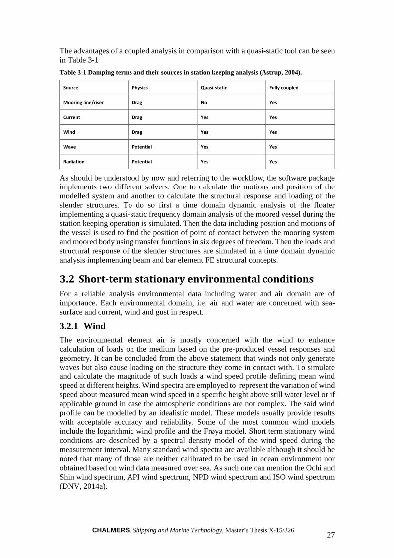
The advantages of a coupled analysis in comparison with a quasi-static tool can be seen
in Table 3-1
Table 3-1 Damping terms and their sources in station keeping analysis (Astrup, 2004).
Source Physics Quasi-static Fully coupled
Mooring line/riser Drag No Yes
Current Drag Yes Yes
Wind Drag Yes Yes
Wave Potential Yes Yes
Radiation Potential Yes Yes
As should be understood by now and referring to the workflow, the software package
implements two different solvers: One to calculate the motions and position of the
modelled system and another to calculate the structural response and loading of the
slender structures. To do so first a time domain dynamic analysis of the floater
implementing a quasi-static frequency domain analysis of the moored vessel during the
station keeping operation is simulated. Then the data including position and motions of
the vessel is used to find the position of point of contact between the mooring system
and moored body using transfer functions in six degrees of freedom. Then the loads and
structural response of the slender structures are simulated in a time domain dynamic
analysis implementing beam and bar element FE structural concepts.
3.2 Short-term stationary environmental conditions
For a reliable analysis environmental data including water and air domain are of
importance. Each environmental domain, i.e. air and water are concerned with sea-
surface and current, wind and gust in respect.
3.2.1 Wind
The environmental element air is mostly concerned with the wind to enhance
calculation of loads on the medium based on the pre-produced vessel responses and
geometry. It can be concluded from the above statement that winds not only generate
waves but also cause loading on the structure they come in contact with. To simulate
and calculate the magnitude of such loads a wind speed profile defining mean wind
speed at different heights. Wind spectra are employed to represent the variation of wind
speed about measured mean wind speed in a specific height above still water level or if
applicable ground in case the atmospheric conditions are not complex. The said wind
profile can be modelled by an idealistic model. These models usually provide results
with acceptable accuracy and reliability. Some of the most common wind models
include the logarithmic wind profile and the Frøya model. Short term stationary wind
conditions are described by a spectral density model of the wind speed during the
measurement interval. Many standard wind spectra are available although it should be
noted that many of those are neither calibrated to be used in ocean environment nor
obtained based on wind data measured over sea. As such one can mention the Ochi and
Shin wind spectrum, API wind spectrum, NPD wind spectrum and ISO wind spectrum
(DNV, 2014a).

CHALMERS, Shipping and Marine Technology, Master’s Thesis X-15/326 28
It should be noted that no matter which profile is used the reliability holds for stable
weather conditions where no severe direction or mean speed changes are recorded. The
only wind profile supported by the SIMO package is the power law wind profile.
The power law wind profile states that (SIMO, 2012a):
𝑈(𝑧) = 𝑈(𝐻)(𝑧
𝐻)𝛼 (30)
Where
𝑧 Height above still water level
𝐻 Reference height
𝑈(𝐻) Mean wind speed at reference height
Before introducing the applied wind spectrum one has to understand the rationalization
of employing a spectral density function to model winds and the reason behind it.
The wind includes two components: a steady component stable over short measurement
intervals known as mean wind speed and a fluctuating portion or in other words the
natural variability around the mean speed. This component also known as turbulence is
defined as fluctuation around the mean wind speed measured at standard height of 10
meters in 10 minute intervals and in statistical terms introduced as the standard
deviation of the wind speed. The interval duration of 10 minutes can differ from
sampling method to sampling method (SIMO, 2012a).
The 10 minute wind speed and its standard deviation refer to the longitudinal direction
(main or constant wind direction) during the measured interval of 10 minutes. It is of
value to note that there is lateral and vertical turbulence perpendicular to wind direction
with mean wind speed of zero which will not be accounted for due to modelling
incapability of the software. While this modelling limitation carries negligible effects
it has root in mathematical modelling of the wind gust. In order to simulate the available
standard wind spectra in time domain a state space model driven by white noise is
implemented, in which a given wind spectrum is first non-dimensionalized by a rational
transfer function. The second step would be the iterative estimation of model
parameters through least square fitting of rational functions to the original model which
helps derive the transfer functions and finally the state space model.
In the present case considering the location and specific characteristics of the API
recommended ISO wind spectrum defined in ISO 19901-1 is used. The ISO spectrum
in fact is the same as the NPD (Norwegian Petroleum Directorate) limited to a
frequency range of 0.00167<f<0.5 (Hz) (SIMO, 2012a).
Although API suggests the use of gust factors profile and spectra recommended by
Norwegian Petroleum Directorate, due to the software limitations here only the
spectrum itself is used.
The dimensional NPD wind energy spectrum at height Z is given as (DNV, 2014a):
𝑆(𝑓) =320 (
𝑣10̅̅ ̅̅10
)2
(𝑧
10)
0.45
(1 + 𝑓0.468)3.561 (31)
Where
CHALMERS, Shipping and Marine Technology, Master’s Thesis X-15/326 29
𝑓 =172𝑓 (
𝑧10
)2 3⁄
(�̅�
10)
3 4⁄ (32)
𝑧 Height over mean water level
�̅� Mean wind speed
v10 Wind speed at 10 meters above mean water level
3.2.2 Water domain
The environmental element water entails wave environment and current effects through
the whole depth of the simulated domain. Considering the fact that current is simulated
as a function varying by depth there is not much to be concerned about other than the
magnitude of velocities with respect to depth. On the other hand the process of
simulating waves based on any chosen wave spectrum in time series may as well be the
most important factor in mooring involved cases especially when fatigue damage is of
interest. The sensitivity of the case heightens in case of simulating extreme conditions,
which are the goal in design process of mooring systems.
Current
The currents move in the horizontal direction but vary with depth. There are various
different types of current. The most common types of current include, wind generated
currents, tidal currents, circulational currents, loop and eddy currents, soliton currents
and longshore currents. As could be comprehended from the name wind generated
currents are caused by wind induced energy, tidal currents are regular occurrences
caused by astronomical motion of the planet. These types of currents are weak in deep
waters but strengthened along coastal areas. The circulational currents or oceanic
currents are large scale currents of the oceanic circulation. The variation of velocity
over depth is highly dependent on site specific ocean data such as climate, vertical
density distribution and flow of water.
In most cases it is sufficient to consider the current as a steady flow field where the
velocity changes are only effected by depth. For an accurate model of currents the
current magnitude should be a summation of all present current types, i.e. wind
generated, tidal and circulational currents.
The design current profile in case of no available site specific measurements can be
assumed to comply with an idealistic models as follows.
The tidal current velocity vector can be modelled as a simple power law where (DNV,
2014a):
𝑉𝑐,𝑡𝑖𝑑𝑒(𝑧) = 𝑉𝑐,𝑡𝑖𝑑𝑒(0) (
𝑑 + 𝑧
𝑑)
𝛼
𝑓𝑜𝑟 𝑧 ≤ 0 (33)
The variation of wind generated currents can be modeled as linear model only effected
by depth. It is common practice to assume wind generated currents fade away lower
than a specific depth d0. The said depth can be considered to be 50 meters from still
water level (DNV, 2014a). The velocity profile is formulated as in equation (34):
𝑉𝑐,𝑤𝑖𝑛𝑑(𝑧) = 𝑉𝑐,𝑤𝑖𝑛𝑑(0) (
𝑑0 + 𝑧
𝑑0) 𝑓𝑜𝑟 − 𝑑0 ≤ 𝑧 ≤ 0 (34)
CHALMERS, Shipping and Marine Technology, Master’s Thesis X-15/326 30
In case of insufficient statistical data, and a location over deep water along an open
coast line the wind generated current velocity at still water level shall be obtained as
follows:
𝑉𝑐,𝑤𝑖𝑛𝑑(0) = 𝑘 ∗ (𝑈1 ℎ𝑜𝑢𝑟,10 𝑚) (35)
The constant 𝑘 in equation (35) can be considered to have a value of 0.015 to 0.030. In
this case 𝑘 is considered to be equal to 0.030 and the total magnitude of current Vc(z)
would become:
𝑉𝑐(𝑧) = 𝑉𝑐,𝑤𝑖𝑛𝑑(𝑧) + 𝑉𝑐,𝑡𝑖𝑑𝑒(𝑧) (36)
𝑧 Vertical distance from still water level, positive upwards
𝑉𝑐,𝑤𝑖𝑛𝑑(0) Wind generated current velocity at still water level
𝑉𝑐,𝑡𝑖𝑑𝑒(0) Tidal current velocity at still water level
𝑑 Absolute value of water depth
𝑑0 Reference depth for wind generated current, can be taken as 50 m
𝛼 Power law exponent most common to take value of 1.7
Waves
Waves act as the source of excitation forces for floating structures at wave frequency
and nonlinear wave forces, e.g. low frequency drift force and second order forces. On
the other hand they apply a nonlinear force on the structure by causing variable wetted
surface of the structure. Considering this fact a reliable wave model with acceptable
accuracy is necessary.
Considering the random and irregular nature of ocean waves in all aspects a sea state is
best modelled by a random wave model. This random and irregular shape has root in
the fact that ocean waves are composed of waves with a mathematically infinite band
of frequencies and various directions. The interaction and interference of waves cause
difficulties in the mathematical modelling of the ocean surface. Various simplified
wave theories and wave spectra are available e.g. Airy waves, second and fifth order
Stokes waves and irregular waves represented by wave spectra such as the JONSWAP,
Pierson Moskowitz, TMA and etc.
Most energy on ocean surface is due to wind blown over a vast area or in other words
wind waves. A wind sea is a wind induced wave system. The so called fully developed
sea is the condition where the waves have matured to a point where for the current mean
wind speed cannot grow any larger and their height and length have reached their
maxima.
In case of structures with significant dynamic response the suggested approach is a time
domain simulation of ocean surface by stochastic means. This process is applicable by
use of a sea state from a wave spectrum with the assumption that it is a stationary
random process.
Short term irregular sea states are described by a wave spectrum or in other words a
power spectral density function. The energy density E is the sum of kinetic and potential
harmonic wave energy over a frequency band per unit area. To translate the wave
spectrum into wave time series a common practice and the method used in the utilized
software package is implementing a FFT formulation based on the algorithm proposed
by Cooley and Tukey (1965).

CHALMERS, Shipping and Marine Technology, Master’s Thesis X-15/326 31
The wave spectrum used in the simulation is the Pierson-Moskowitz wave spectrum.
The Pierson-Moskowitz is based on measurements in North Atlantic and is one of the
simplest descriptions of energy distribution.
The Pierson-Moskowitz spectrum is defined as (SIMO, 2012a):
𝑆𝜉
+(𝜔) =𝛼
𝜔5𝑒𝑥𝑝 (
−𝑏
𝜔4) (37)
Where the constants 𝛼 and 𝑏 for the two-parameter spectrum can be defined as:
𝑏 = (
2𝜋
𝑇𝑧)
4
𝜋 = 496.1⁄ /𝑇𝑧4
𝛼 = 𝑏𝐻𝑠2 4⁄ = 124𝐻𝑠
2 𝑇𝑧4⁄
(38)
And
𝐻𝑠 Specific wave height
𝑇𝑧 Zero up-crossing wave period
3.3 Long-term statistics
As mentioned before for an FLS study of a station keeping operation the environmental
data implemented in the simulation should be site specific. While such data was not at
hand, the statistical approach to the issue, based on regulatory recommendations (DNV,
2014a), is used.
Waves
As was mentioned in section 2.4 the random variable Z is chosen to be Gaussian. To be
able to use Legendre-Gauss integral scheme the zi are chosen to be the abscissae of the
accuracy n=20. Considering that the interval of the integral calculating cj term of the
Wiener chaos expansion is infinite here the intervals are chosen to be [-4 4]. By using
equation (25) the integral interval is transformed to Legendre-Gauss bounds. The
weight and abscissae of the chosen Gaussian quadrature should be multiplied
by 𝑏 − 𝑎 2⁄ , in this case 4. By doing so the abscissae of the quadrature become the
normal random variable zi and the weights – hi. In this study it is chosen to study the
dependence of fatigue damage on Hs, the specific wave height of the Pierson-
Moskowitz wave spectrum. Hence the zi becomes the standard normal random variable
representing specific wave height.
On the other hand based on environmental condition recommendations (DNV, 2014a)
and based on the following CMA joint model it is suggested that the significant wave
height is to be modelled by a 3-parameter Weibull distribution with density function of:
𝑓𝐻𝑠
(ℎ) =𝛽𝐻𝑠
𝛼𝐻𝑠
(ℎ − 𝛾𝐻𝑠
𝛼𝐻𝑠
)
𝛽𝐻𝑠−1
𝑒𝑥𝑝 {(ℎ − 𝛾𝐻𝑠
𝛼𝐻𝑠
)
𝛽𝐻𝑠
} (39)
Where 𝛼𝐻𝑠 and 𝛽𝐻𝑠
are the scale and shape parameters of the Weibull distribution and
using the data provided by the recommended practice regarding environmental
conditions (DNV, 2014a) the parameter γ is assumed to be zero.
CHALMERS, Shipping and Marine Technology, Master’s Thesis X-15/326 32
Following the fact that the random variable is supposed to be Gaussian and the specific
wave height belonging to a Weibull distribution here the cdf of each standard normal
random variable is used to get the respective specific wave height utilizing a Weibull
inverse scheme with suggested shape and scale parameters.
Considering the fact that the wave environment is simulated by a two-parameter
Pierson-Moskowitz spectrum the other required parameter is Tp the peak period. To
calculate the peak period we first calculate the zero up-crossing wave period. The Tz is
assumed to follow a lognormal distribution conditional on specific wave height (DNV,
2014a).
𝑓𝑇𝑧|𝐻𝑠
(𝑡|ℎ) =1
𝜎𝑡√2𝜋𝑒𝑥𝑝 {
(𝑙𝑛𝑡 − 𝜇)2
2𝜎2} (40)
Where:
𝜇 = 𝐸[𝑙𝑛𝑇𝑧] = 𝑎0 + 𝑎1ℎ𝑎2
𝜎 = 𝑠𝑡𝑑[𝑙𝑛𝑇𝑧] = 𝑏0 + 𝑏1ℎℎ𝑏2
In the above equations the constants 𝑎𝑖 , 𝑏𝑖 with i=0, 1, 2 are estimated from field
measurements.
After obtaining values of Tz for individual sea states the peak periods are calculated
assuming that 𝑇𝑝 = 1.408𝑇𝑧 (Brodtkorb, 2000).
Wind
Based on the studies of Johannessen (Johannessen, 2002) on the wind measurements
from the Northern North Sea, the mean wind speed fits best to a Weibull distribution.
A Weibull distribution has the form of the following equation:
𝐹(𝑊) = 1 − exp [− (
𝑊
𝛽)
𝛼
] (41)
Where 𝛼 and 𝛽 are the shape and scale parameters of the distribution.
On the other hand there are approaches based on joint distribution of specific wave
height and wind mean velocity (Li, 2015). Based on DNV regulations on environmental
conditions the said joint distribution can be defined as a two parameter Weibull
distribution as well (DNV, 2014a).
𝑓𝑈|𝐻𝑠
(𝑢|ℎ) = 𝑘𝑢𝑘−1
𝑈𝑐𝑘 𝑒𝑥𝑝[−(
𝑢
𝑈𝐶)𝑘] (42)
Here scale parameter 𝑈𝐶 and shape parameter k are calculated from field data. The
formulation is as follows:
𝑘 = 𝑐1 + 𝑐2ℎ𝑠𝑐3 & 𝑈𝑐 = 𝑐4 + 𝑐5ℎ𝑠
𝑐6 (43)
The parameters of the above equations are obtained by nonlinear curve fitting of field
measurements (Li, 2015). Although the second approach will definitely provide more
realistic results as the parameters for the joint wind specific wave height are not
available the same method used to obtain specific wave heights from the standard
CHALMERS, Shipping and Marine Technology, Master’s Thesis X-15/326 33
normal random variables is applied for procuring the wind speed in agreement with the
sea state.
3.4 Simulation process
The contents of this section include the workflow of the software package and the
interaction of different toolboxes; implemented parameters of the analysis will be
presented based on the theoretical background discussed in chapter three. In the end the
effective tension obtained from the analysis of a chosen line will be presented. These
results will be used to estimate the fatigue using spectral methods and direct rainflow
counting of stress cycles. Damage of the line and will be implemented in the long-term
fatigue damage approximation by both WCE and Gaussian approximation.
3.4.1 Workflow and DeepC toolsets
The interactive software DeepC (deep water coupled vessel motion analysis), used for
floating body configurations attached to seabed utilizes the programs SIMO and
RIFLEX developed by MARINTEK. The two programs utilize the time domain
coupled analysis (DNV, 2014b). The DeepC package uses input files from
HydroD/Wadam to facilitate time domain analysis based on the hydrodynamic data
obtained from the named programs. The software also accepts a FE physical model of
the vessel or any floating bodies which is merely for visualization purposes (DNV,
2014b). DeepC in addition to a built in cable solver provides a range of post processing
capabilities including but not limited to 2D statistical and result plots and 3D contour
plots of static and fatigue analysis results (DNV, 2014b).
DeepC being an integrated part of the DNV software package SESAM needs input files
from other integrated programs. Prior to modelling in DeepC one needs the geometry
of large volume floaters and hydrostatic and dynamic data including frequency domain
added mass and potential damping and excitation forces of first and second order (DNV,
2014b).
As mentioned DeepC is a time domain coupled analysis program. On the other hand
the input data from Wadam and the simulation process in SIMO is frequency domain.
To provide results in time domain the package uses FFT method to transfer data from
frequency domain to time domain. This process requires cautious in the modelling
process in previous steps so that the frequency domain characteristics properly cover
all frequency intervals with notable energy content.
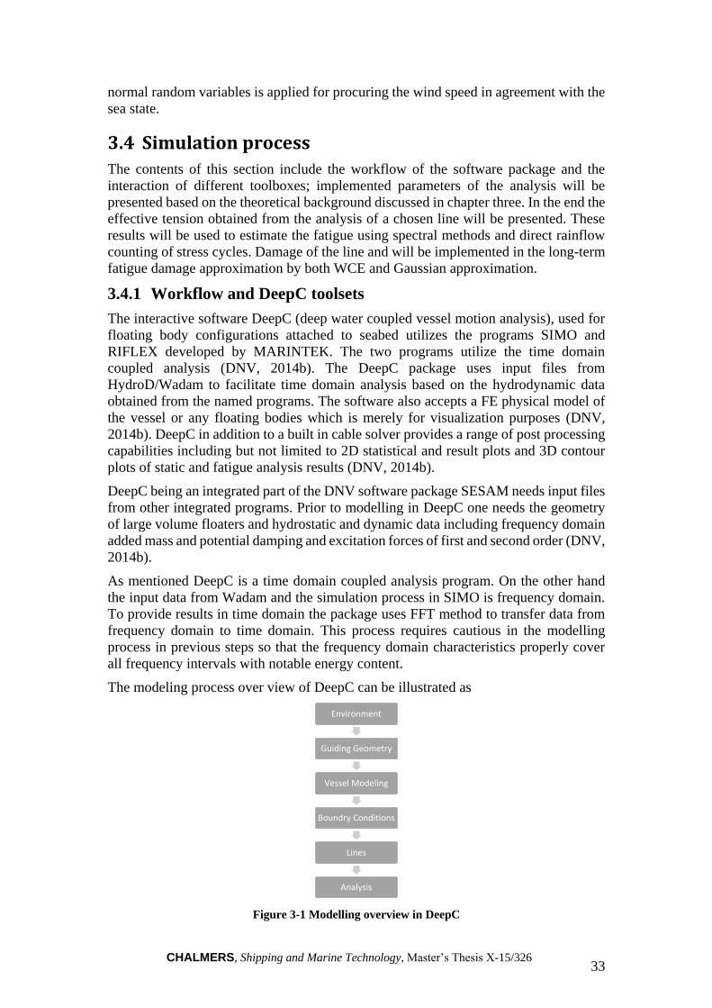
The modeling process over view of DeepC can be illustrated as
Figure 3-1 Modelling overview in DeepC
Environment
Guiding Geometry
Vessel Modeling
Boundry Conditions
Lines
Analysis

CHALMERS, Shipping and Marine Technology, Master’s Thesis X-15/326 34
The whole modelling loop in the software package SESAM towards undertaking of a
coupled analysis can be visualised in the following order.
Figure 3-2 Modelling loop
The modelling process in DeepC includes utilizing the two programs SIMO and
RIFLEX.
Both integrated programs, SIMO and RIFLEX are designed so that they can be used
separately and do have capabilities that are not included in the current interface of
DeepC, such as DP modelling and way point tracking capabilities included in SIMO.
In the scope of the present thesis work the two programs are utilized only through the
DeepC interface as the GUI capabilities suffice for the study. Noting the mentioned fact
it is important to have a realization of the simulation process of both software to explain
the workflow of DeepC.
SIMO developed by MARINTEK for DNV Software is the DeepC module for flexible
modelling of station keeping and connecting mechanisms. The software is capable of
simulating complex multi-body systems (DNV.GL, 2015a). The program itself consists
of five modules: INPMOD, STAMOD, DYNMOD, OUTMOD, and PLOMOD. The
named modules are used for reading system description, running static analysis and
defining initial condition, generating time series and dynamic analysis of the system,
post processing of the simulation output data and time series and finally plotting of the
results in respect to the above order. The work flow and related file formats of SIMO
can be illustrated as:
Figure 3-3 SIMO program system and file communication (SIMO, 2012b)
Create FEM panel model of large structures
Run HydroD to calculate added mass, potential
damping, excitation
forces, etc. using potential
theory
DeepC simulation
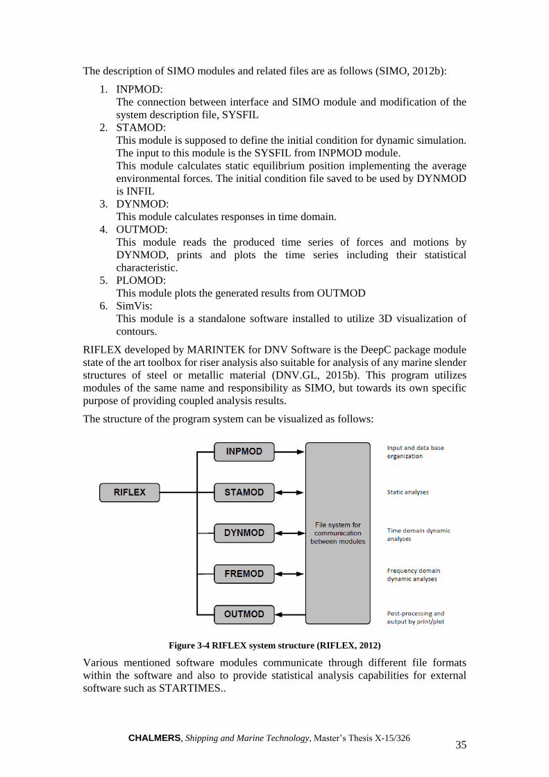
CHALMERS, Shipping and Marine Technology, Master’s Thesis X-15/326 35
The description of SIMO modules and related files are as follows (SIMO, 2012b):
1. INPMOD:
The connection between interface and SIMO module and modification of the
system description file, SYSFIL
2. STAMOD:
This module is supposed to define the initial condition for dynamic simulation.
The input to this module is the SYSFIL from INPMOD module.
This module calculates static equilibrium position implementing the average
environmental forces. The initial condition file saved to be used by DYNMOD
is INFIL
3. DYNMOD:
This module calculates responses in time domain.
4. OUTMOD:
This module reads the produced time series of forces and motions by
DYNMOD, prints and plots the time series including their statistical
characteristic.
5. PLOMOD:
This module plots the generated results from OUTMOD
6. SimVis:
This module is a standalone software installed to utilize 3D visualization of
contours.
RIFLEX developed by MARINTEK for DNV Software is the DeepC package module
state of the art toolbox for riser analysis also suitable for analysis of any marine slender
structures of steel or metallic material (DNV.GL, 2015b). This program utilizes
modules of the same name and responsibility as SIMO, but towards its own specific
purpose of providing coupled analysis results.
The structure of the program system can be visualized as follows:
Figure 3-4 RIFLEX system structure (RIFLEX, 2012)
Various mentioned software modules communicate through different file formats
within the software and also to provide statistical analysis capabilities for external
software such as STARTIMES..

CHALMERS, Shipping and Marine Technology, Master’s Thesis X-15/326 36
Now that the responsibility and work process of the modules are defined the workflow
of the DeepC interface can be discussed. Simply put the non-linear analysis is
performed in two steps:
1. Static equilibrium analysis: starting from the stress free coordinates calculated
by the built-in cable solver the software will end up with the line end points
calculating the forces in a pre-specified number of load steps.
2. Dynamic analysis: starting from the static equilibrium position calculated in
STAMOD the related modules perform a time domain analysis of the system
based on the specified environmental conditions and headings.
For a better understanding of the above process one can refer to Figure 3-5.
Figure 3-5 DeepC workflow

CHALMERS, Shipping and Marine Technology, Master’s Thesis X-15/326 37

CHALMERS, Shipping and Marine Technology, Master’s Thesis X-15/326 38
4 Case study FPSO and associated mooring system
The geometry and hydrodynamic data used in the present work is the provided example
model by the software. The vessel is an FPSO with the following properties:
Table 4-1 Model properties of FPSO
Length over all (LOA) 224 (m)
Draught 16 (m)
Breadth 41 (m)
Figure 4-1 Perspective view of case study FPSO
The vessel is floating over 900 meters of water, internal turret moored to seabed
utilizing a semi-taut 12 line mooring arrangement. The lines are divided into groups of
three, 15 degrees apart and 90 degrees between each group. In this set up to have a more
realistic condition considering that fact that risers cause high frequency excitation
forces in deep-water production units 4 risers are modelled in addition to the mooring
system. The mooring system design of having the lines in groups provides redundancy,
but causes some concern regarding fatigue life of individual lines. Since the tension-
tension acting on lines are very similar in each group the fatigue life of components are
also close which asks for extra cautious regarding inspection schedule. The lines are
composed of a fairlead and seabed stud chain and a spiral strand wire rope. The steel is
chosen as grade NV R4. It should be noted that the material does not have any effect
on the estimated fatigue damage as the applied method implements the guidelines based
on S-N curves. This oversight is of course in contradiction with reality. The steel grade
is only chosen to fulfill safety margins of the guidelines.
As mentioned the FPSO uses a single point mooring system utilizing an internal turret.
In an internal turret moored FPSO the turret structure is installed permanently or
detachable inside the tanker’s hull and is connected to seabed in a CALM (Catenary
Anchor Leg Mooring) arrangement. This set up allows the vessel to weathervane in
reaction to varying environmental conditions and directions (Rajesh, 2006). The free
rotating character of the moored vessel is modelled as ball joint at the connection point
of the vessel to the mooring lines.
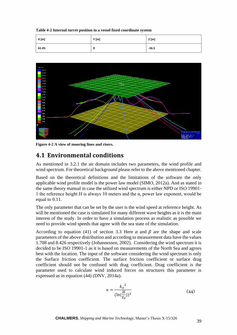
CHALMERS, Shipping and Marine Technology, Master’s Thesis X-15/326 39
Table 4-2 Internal turret position in a vessel fixed coordinate system
X [m] Y [m] Z [m]
61.45 0 -16.5
Figure 4-2 A view of mooring lines and risers.
4.1 Environmental conditions
As mentioned in 3.2.1 the air domain includes two parameters, the wind profile and
wind spectrum. For theoretical background please refer to the above mentioned chapter.
Based on the theoretical definitions and the limitations of the software the only
applicable wind profile model is the power law model (SIMO, 2012a). And as stated in
the same theory manual in case the utilized wind spectrum is either NPD or ISO 19901-
1 the reference height H is always 10 meters and the α, power law exponent, would be
equal to 0.11.
The only parameter that can be set by the user is the wind speed at reference height. As
will be mentioned the case is simulated for many different wave heights as it is the main
interest of the study. In order to have a simulation process as realistic as possible we
need to provide wind speeds that agree with the sea state of the simulation.
According to equation (41) of section 3.3 Here 𝛼 and 𝛽 are the shape and scale
parameters of the above distribution and according to measurement data have the values
1.708 and 8.426 respectively (Johannessen, 2002). Considering the wind spectrum it is
decided to be ISO 19901-1 as it is based on measurements of the North Sea and agrees
best with the location. The input of the software considering the wind spectrum is only
the Surface friction coefficient. The surface friction coefficient or surface drag
coefficient should not be confused with drag coefficient. Drag coefficient is the
parameter used to calculate wind induced forces on structures this parameter is
expressed as in equation (44) (DNV, 2014a).
𝜅 =
𝑘𝑎2
(ln (𝐻𝑧0
))2 (44)

CHALMERS, Shipping and Marine Technology, Master’s Thesis X-15/326 40
Where:
𝜅 The surface friction coefficient
𝑘𝑎 The von Karman’s constant equal to 0.4
H The reference height here equal to 10 meters
𝑧0 The terrain roughness parameter for open seas takes value of 0.0001 to 0.01
Considering the above mentioned formulation the input for the wind spectrum is
calculated to be 𝜅 = 0.0033
If the applied wind spectrum is API, NPD and or ISO 19901-1 the H should be set to
10 meters and for α height coefficient, which normally takes a value of 0.1 to 0.14,
should be set to constant of 0.11.
For a detailed presentation of the applied environmental conditions regarding wind
speed please refer to Table 4-4.
4.1.1 Water domain
In order to simulate the water surface and connected environmental parameters there
are two matters that should be taken care of. For the theoretical background needed for
all subjects included in this section please refer to 3.2.2.
As mentioned in 3.3 the specific wave height follows a three-parameter Weibull
distribution with scale and shape parameters depending on site specific data. As the
case study here is chosen to be located in North Sea the scale and shape parameters
taken from DNV recommended practice on environmental conditions (DNV, 2014a)
are 𝛼𝐻𝑠= 2.19 and 𝛽𝐻𝑠
= 1.26, while 𝛾 = 0. To calculate the zero-crossing period,
Tz, dependent on specific wave height the standard deviation and mean of the lognormal
distribution are needed (DNV, 2014a). To obtain the two parameters, 𝜎 and 𝜇, equation
(40) of section 3.3 is used. The constants as recommended are presented in Table 4-3.
Table 4-3 Constants used to calculate mean and standard deviation of the joint zero up-crossing
period and wave height lognormal distribution (DNV, 2014a)
𝒂𝟎 𝒂𝟏 𝒂𝟐 𝒃𝟎 𝒃𝟏 𝒃𝟐
0.7 0.935 0.222 0.07 0.1386 -0.0208
The current data applied as a parameter in the simulation is based on the relations and
theoretical background mentioned in 3.2.2. As can be observed from the related
formulation to capacitate the calculation of current in different depths there is a need of
current velocity in water surface. The said magnitude is chosen based on the guidelines
of environmental conditions in DNV (DNV, 2014a) and is equal to 1.5𝑚 𝑠⁄ .
The environmental data for each of the 20 sea states simulated as part of the study and
obtained based on the procedures included in 3.3 and this section earlier are presented
in Table 4-4.
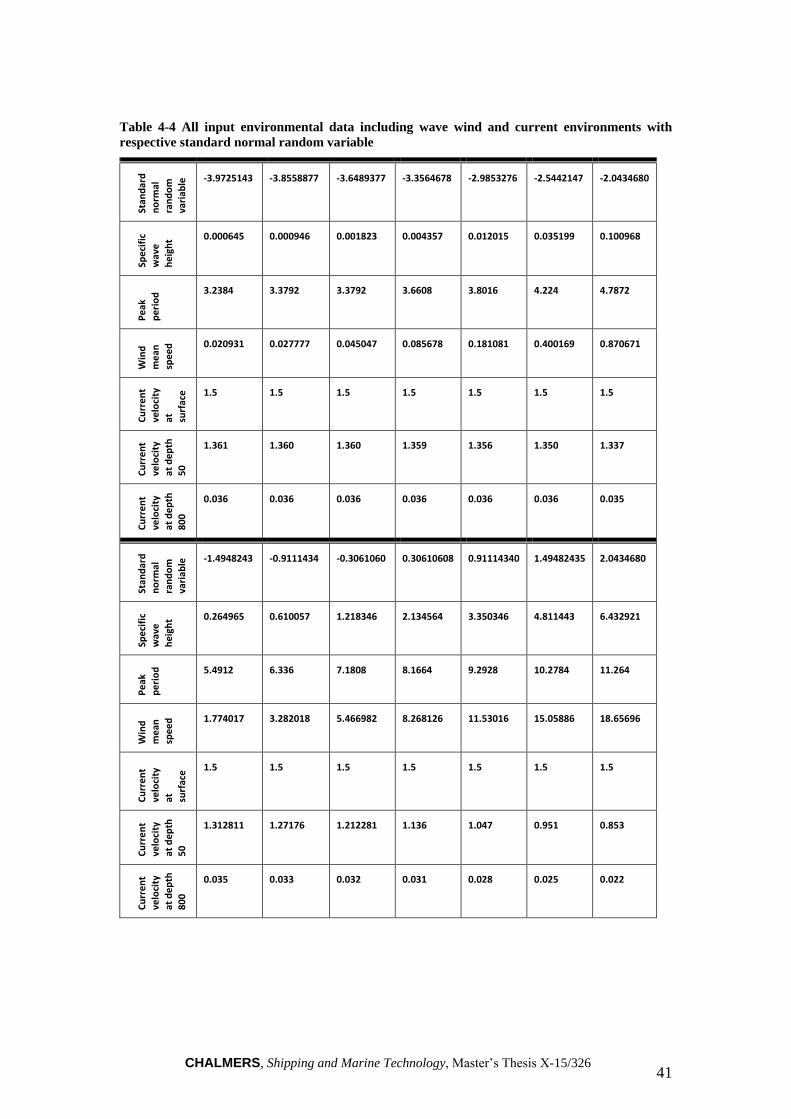
CHALMERS, Shipping and Marine Technology, Master’s Thesis X-15/326 41
Table 4-4 All input environmental data including wave wind and current environments with
respective standard normal random variable St
and
ard
no
rmal
ran
do
m
vari
able
-3.9725143 -3.8558877 -3.6489377 -3.3564678 -2.9853276 -2.5442147 -2.0434680
Spe
cifi
c
wav
e
he
igh
t 0.000645 0.000946 0.001823 0.004357 0.012015 0.035199 0.100968
Pe
ak
pe
rio
d 3.2384 3.3792 3.3792 3.6608 3.8016 4.224 4.7872
Win
d
me
an
spe
ed
0.020931 0.027777 0.045047 0.085678 0.181081 0.400169 0.870671
Cu
rre
nt
velo
city
at
surf
ace
1.5 1.5 1.5 1.5 1.5 1.5 1.5
Cu
rre
nt
velo
city
at d
ep
th
50
1.361 1.360 1.360 1.359 1.356 1.350 1.337
Cu
rre
nt
velo
city
at d
ep
th
80
0
0.036 0.036 0.036 0.036 0.036 0.036 0.035
Stan
dar
d
no
rmal
ran
do
m
vari
able
-1.4948243 -0.9111434 -0.3061060 0.30610608 0.91114340 1.49482435 2.0434680
Spe
cifi
c
wav
e
he
igh
t 0.264965 0.610057 1.218346 2.134564 3.350346 4.811443 6.432921
Pe
ak
pe
rio
d
5.4912 6.336 7.1808 8.1664 9.2928 10.2784 11.264
Win
d
me
an
spe
ed
1.774017 3.282018 5.466982 8.268126 11.53016 15.05886 18.65696
Cu
rre
nt
velo
city
at
surf
ace
1.5 1.5 1.5 1.5 1.5 1.5 1.5
Cu
rre
nt
velo
city
at d
ep
th
50
1.312811 1.27176 1.212281 1.136 1.047 0.951 0.853
Cu
rre
nt
velo
city
at d
ep
th
80
0
0.035 0.033 0.032 0.031 0.028 0.025 0.022
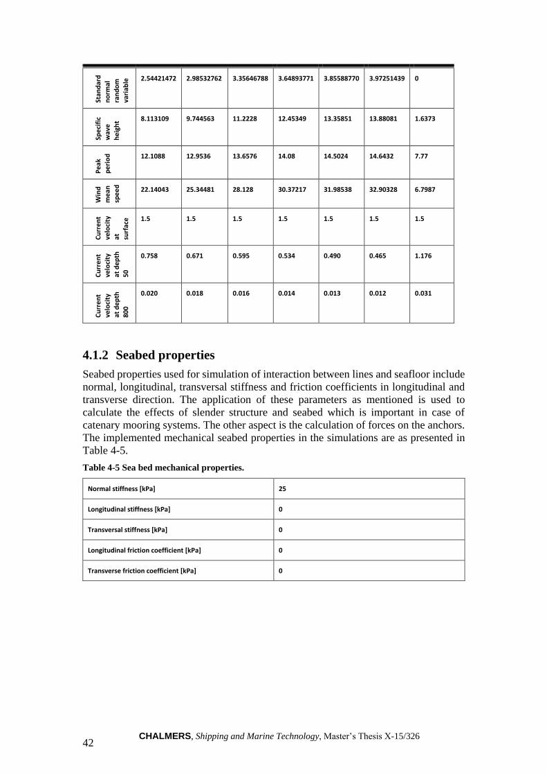
CHALMERS, Shipping and Marine Technology, Master’s Thesis X-15/326 42
Stan
dar
d
no
rmal
ran
do
m
vari
able
2.54421472 2.98532762 3.35646788 3.64893771 3.85588770 3.97251439 0
Spe
cifi
c
wav
e
he
igh
t 8.113109 9.744563 11.2228 12.45349 13.35851 13.88081 1.6373
Pe
ak
pe
rio
d
12.1088 12.9536 13.6576 14.08 14.5024 14.6432 7.77
Win
d
me
an
spe
ed
22.14043 25.34481 28.128 30.37217 31.98538 32.90328 6.7987
Cu
rre
nt
velo
city
at
surf
ace
1.5 1.5 1.5 1.5 1.5 1.5 1.5
Cu
rre
nt
velo
city
at d
ep
th
50
0.758 0.671 0.595 0.534 0.490 0.465 1.176
Cu
rre
nt
velo
city
at d
ep
th
80
0
0.020 0.018 0.016 0.014 0.013 0.012 0.031
4.1.2 Seabed properties
Seabed properties used for simulation of interaction between lines and seafloor include
normal, longitudinal, transversal stiffness and friction coefficients in longitudinal and
transverse direction. The application of these parameters as mentioned is used to
calculate the effects of slender structure and seabed which is important in case of
catenary mooring systems. The other aspect is the calculation of forces on the anchors.
The implemented mechanical seabed properties in the simulations are as presented in
Table 4-5.
Table 4-5 Sea bed mechanical properties.
Normal stiffness [kPa] 25
Longitudinal stiffness [kPa] 0
Transversal stiffness [kPa] 0
Longitudinal friction coefficient [kPa] 0
Transverse friction coefficient [kPa] 0

CHALMERS, Shipping and Marine Technology, Master’s Thesis X-15/326 43

CHALMERS, Shipping and Marine Technology, Master’s Thesis X-15/326 44
5 Results and fatigue damage approximation
In this chapter, the results of the time domain simulation of the system are presented.
Following the previous sections the fatigue damage of the fairlead mooring chain is
estimated using the discussed direct rainflow counting and spectral methods to provide
means of comparison between the two. Further on the fatigue damage calculated by
rainflow counting is used to calculate the parameters of the Wiener chaos expansion
and Gaussian approximation method to evaluate the two methods.
5.1 Results of line force time-series
DeepC provides various options considering the storage of results. The options vary
from saving envelope curves vessel position time series to nodal response of individual
lines. In here to study fatigue damage on lines, one chain serves the same purpose as
having all results. Hence the choice of a single fairlead chain of one randomly selected
line. The provided and used results to obtain the fatigue damage of the chain, known as
effective tension is reported element wise. The element size of the fairlead chain is 50
meters. It should be noted that although out of plane bending has notable effect on the
damage rate of mooring chains the software does not have the capability of calculating
for this factor and is only concerned with longitudinal tension forces on lines. As will
be discussed in detail there are two approaches to rainflow counting of the stress ranges:
one based on the force spectrum and the other direct rainflow counting of the force time
series. Here we choose the direct approach. To visualize and provide a good sense of
the force time series, it will be plotted in a graph beside its force spectrum. The force
time series visualized in figures Figure 5-1 to Figure 5-6 and Appendix A in the first 7
cases show an initial irregularity in loading. This might be due to a condition of unstable
equilibrium as the starting point of the dynamic simulation of the system. Although the
system phases this instability out the accumulated damage of lines for this simulation
conditions is merely due to this initial loads which in the worst case lasts for more than
3000 seconds. After stable equilibrium is reached the stress ranges get reduced to zero
in all the said simulation conditions. The results of three simulation conditions are
presented in Figure 5-1 to Figure 5-6, the calmest sea condition to the most extreme sea
condition. The rest of the force time series can be found in Appendix A – Force time
series and spectral graphs. As is obvious from the figures at the start there is high
fluctuation of forces and the force spectral presentation also shows one peak at the start.
This trend continues up till simulation condition 10 with specific wave height of 1.2
(m) and get resolved on its own from then on. The effect of this slowly varying response
can be seen in the spectral plots where the energy is concentrated in low frequencies.
Figure 5-1 Tension-tension force time series sea-condition three
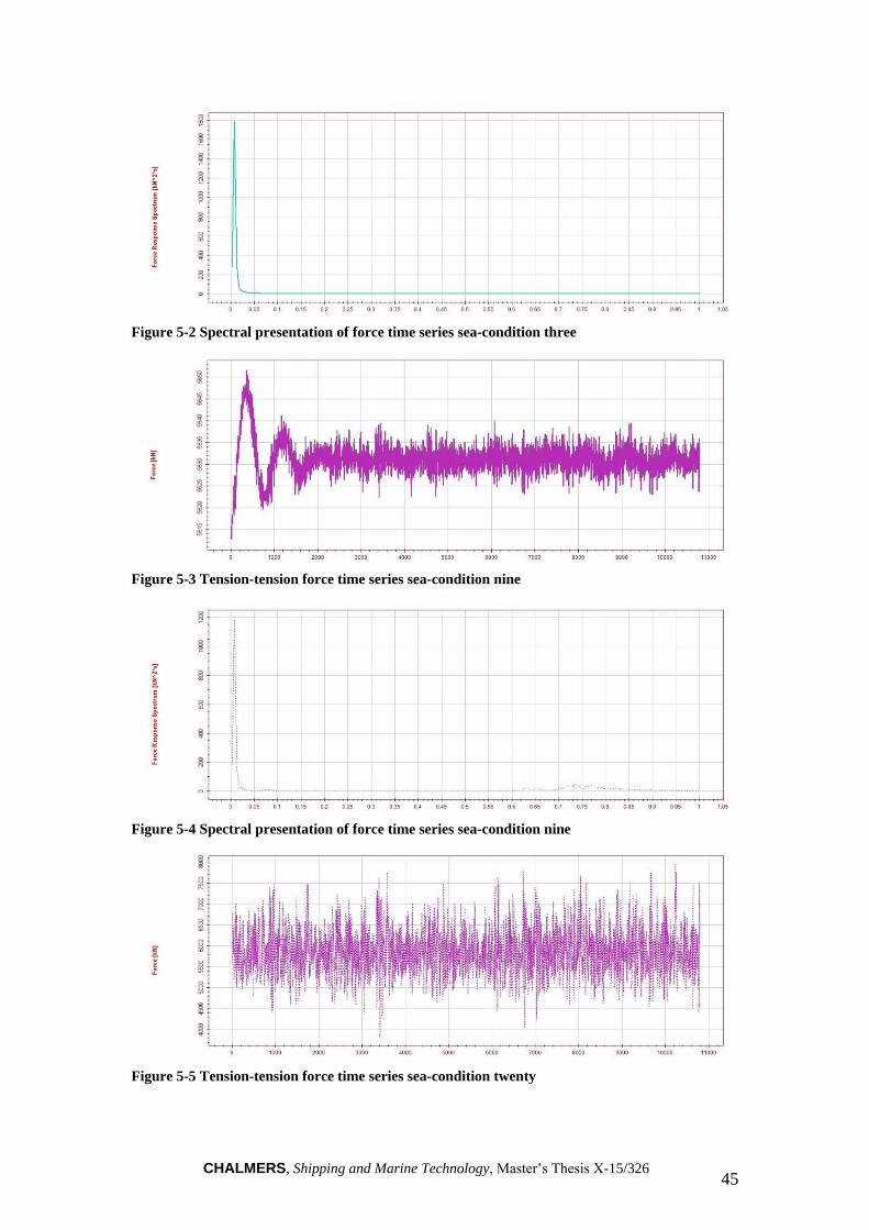
CHALMERS, Shipping and Marine Technology, Master’s Thesis X-15/326 45
Figure 5-2 Spectral presentation of force time series sea-condition three
Figure 5-3 Tension-tension force time series sea-condition nine
Figure 5-4 Spectral presentation of force time series sea-condition nine
Figure 5-5 Tension-tension force time series sea-condition twenty
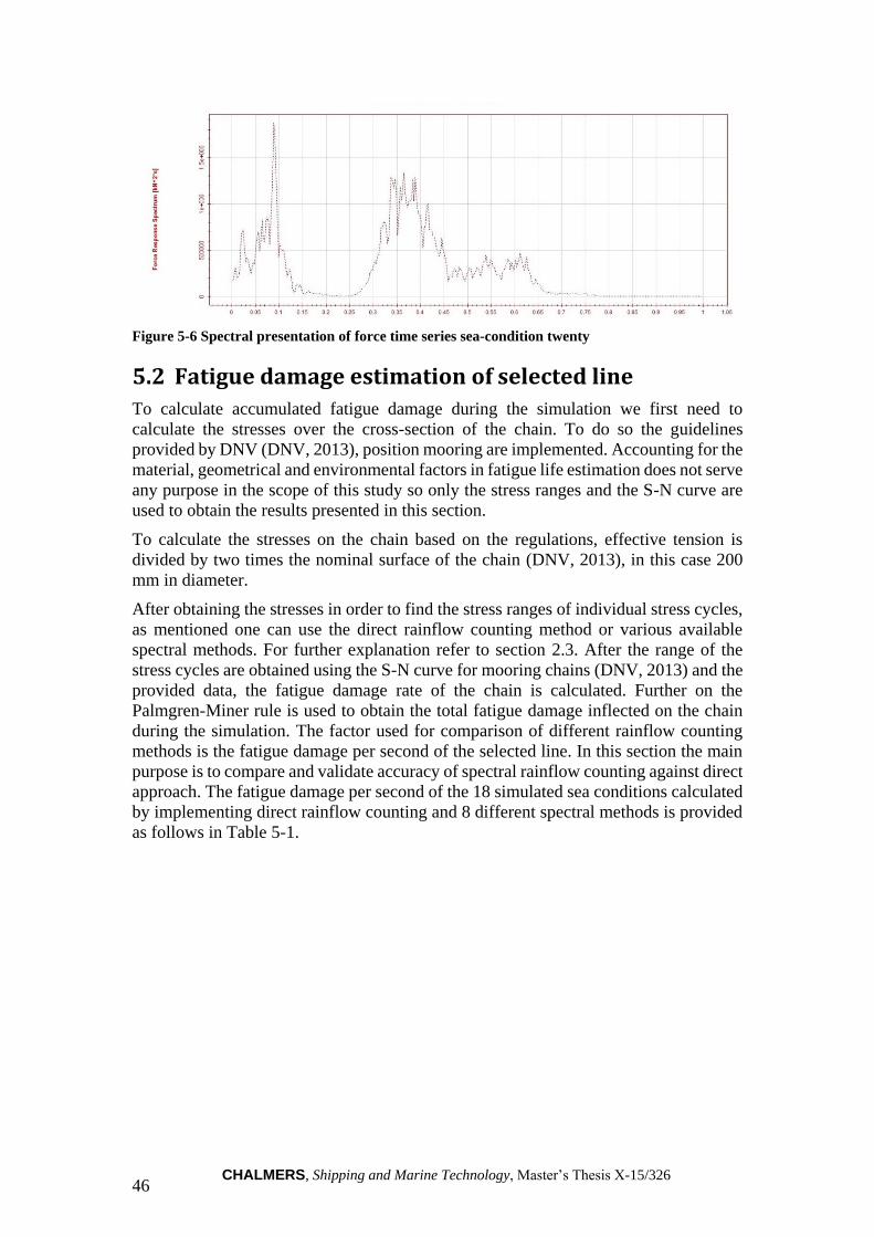
CHALMERS, Shipping and Marine Technology, Master’s Thesis X-15/326 46
Figure 5-6 Spectral presentation of force time series sea-condition twenty
5.2 Fatigue damage estimation of selected line
To calculate accumulated fatigue damage during the simulation we first need to
calculate the stresses over the cross-section of the chain. To do so the guidelines
provided by DNV (DNV, 2013), position mooring are implemented. Accounting for the
material, geometrical and environmental factors in fatigue life estimation does not serve
any purpose in the scope of this study so only the stress ranges and the S-N curve are
used to obtain the results presented in this section.
To calculate the stresses on the chain based on the regulations, effective tension is
divided by two times the nominal surface of the chain (DNV, 2013), in this case 200
mm in diameter.
After obtaining the stresses in order to find the stress ranges of individual stress cycles,
as mentioned one can use the direct rainflow counting method or various available
spectral methods. For further explanation refer to section 2.3. After the range of the
stress cycles are obtained using the S-N curve for mooring chains (DNV, 2013) and the
provided data, the fatigue damage rate of the chain is calculated. Further on the
Palmgren-Miner rule is used to obtain the total fatigue damage inflected on the chain
during the simulation. The factor used for comparison of different rainflow counting
methods is the fatigue damage per second of the selected line. In this section the main
purpose is to compare and validate accuracy of spectral rainflow counting against direct
approach. The fatigue damage per second of the 18 simulated sea conditions calculated
by implementing direct rainflow counting and 8 different spectral methods is provided
as follows in Table 5-1.
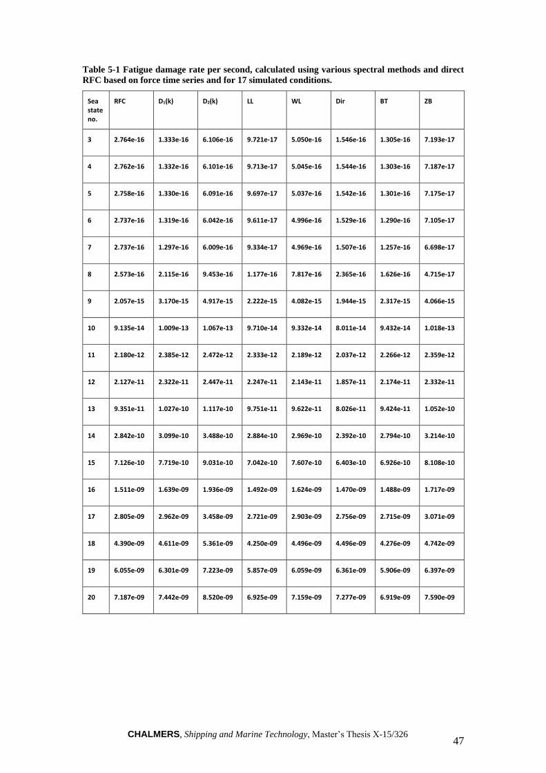
CHALMERS, Shipping and Marine Technology, Master’s Thesis X-15/326 47
Table 5-1 Fatigue damage rate per second, calculated using various spectral methods and direct
RFC based on force time series and for 17 simulated conditions.
Sea state no.
RFC D1(k) D2(k) LL WL Dir BT ZB
3 2.764e-16 1.333e-16 6.106e-16 9.721e-17 5.050e-16 1.546e-16 1.305e-16 7.193e-17
4 2.762e-16 1.332e-16 6.101e-16 9.713e-17 5.045e-16 1.544e-16 1.303e-16 7.187e-17
5 2.758e-16 1.330e-16 6.091e-16 9.697e-17 5.037e-16 1.542e-16 1.301e-16 7.175e-17
6 2.737e-16 1.319e-16 6.042e-16 9.611e-17 4.996e-16 1.529e-16 1.290e-16 7.105e-17
7 2.737e-16 1.297e-16 6.009e-16 9.334e-17 4.969e-16 1.507e-16 1.257e-16 6.698e-17
8 2.573e-16 2.115e-16 9.453e-16 1.177e-16 7.817e-16 2.365e-16 1.626e-16 4.715e-17
9 2.057e-15 3.170e-15 4.917e-15 2.222e-15 4.082e-15 1.944e-15 2.317e-15 4.066e-15
10 9.135e-14 1.009e-13 1.067e-13 9.710e-14 9.332e-14 8.011e-14 9.432e-14 1.018e-13
11 2.180e-12 2.385e-12 2.472e-12 2.333e-12 2.189e-12 2.037e-12 2.266e-12 2.359e-12
12 2.127e-11 2.322e-11 2.447e-11 2.247e-11 2.143e-11 1.857e-11 2.174e-11 2.332e-11
13 9.351e-11 1.027e-10 1.117e-10 9.751e-11 9.622e-11 8.026e-11 9.424e-11 1.052e-10
14 2.842e-10 3.099e-10 3.488e-10 2.884e-10 2.969e-10 2.392e-10 2.794e-10 3.214e-10
15 7.126e-10 7.719e-10 9.031e-10 7.042e-10 7.607e-10 6.403e-10 6.926e-10 8.108e-10
16 1.511e-09 1.639e-09 1.936e-09 1.492e-09 1.624e-09 1.470e-09 1.488e-09 1.717e-09
17 2.805e-09 2.962e-09 3.458e-09 2.721e-09 2.903e-09 2.756e-09 2.715e-09 3.071e-09
18 4.390e-09 4.611e-09 5.361e-09 4.250e-09 4.496e-09 4.496e-09 4.276e-09 4.742e-09
19 6.055e-09 6.301e-09 7.223e-09 5.857e-09 6.059e-09 6.361e-09 5.906e-09 6.397e-09
20 7.187e-09 7.442e-09 8.520e-09 6.925e-09 7.159e-09 7.277e-09 6.919e-09 7.590e-09
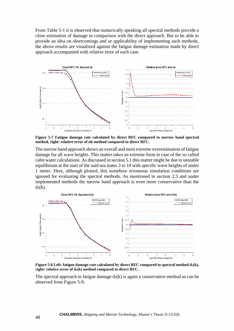
CHALMERS, Shipping and Marine Technology, Master’s Thesis X-15/326 48
From Table 5-1 it is observed that numerically speaking all spectral methods provide a
close estimation of damage in comparison with the direct approach. But to be able to
provide an idea on shortcomings and or applicability of implementing such methods,
the above results are visualized against the fatigue damage estimation made by direct
approach accompanied with relative error of each case.
Figure 5-7 Fatigue damage rate calculated by direct RFC compared to narrow band spectral
method, right: relative error of nb method compared to direct RFC.
The narrow band approach shows an overall and most extreme overestimation of fatigue
damage for all wave heights. This matter takes an extreme form in case of the so called
calm water calculations. As discussed in section 5.1 this matter might be due to unstable
equilibrium at the start of the said sea states 3 to 10 with specific wave heights of under
1 meter. Here, although plotted, this somehow erroneous simulation conditions are
ignored for evaluating the spectral methods. As mentioned in section 2.3 and under
implemented methods the narrow band approach is even more conservative than the
d2(k).
Figure 5-8 Left: fatigue damage rate calculated by direct RFC compared to spectral method d1(k),
right: relative error of d1(k) method compared to direct RFC.
The spectral approach to fatigue damage d2(k) is again a conservative method as can be
observed from Figure 5-9.

CHALMERS, Shipping and Marine Technology, Master’s Thesis X-15/326 49
Figure 5-9 Left: fatigue damage rate calculated by direct RFC compared to spectral method d2(k),
right: relative error of d2(k) method compared to direct RFC.
Figure 5-10 Left: fatigue damage rate calculated by direct RFC and spectral method introduced
by Wirsching and Light, right: relative error of WL method compared to direct RFC.
The WL approximation method implementing 𝛼2, the irregularity factor, created to
reduce the conservativeness of the d2(k) approach is a method introduced by Wirsching
and Light (P. H. Wirsching, Light, M.C., 1980) and shows a closer approximation of
damage in comparison to the previous methods with a much smaller relative error as in
Figure 5-10 right.
Figure 5-11 Left: fatigue damage rate calculated by direct RFC and spectral method introduced
by Lutes and Larsen, right: relative error of LL method compared to direct RFC.

CHALMERS, Shipping and Marine Technology, Master’s Thesis X-15/326 50
The simple approximation proposed by Lutes and Larsen (Lutes, 1990) plotted in
Figure 5-11 shows slight underestimation of fatigue damage in case of sea states with
extreme wave heights.
Figure 5-12 Left: fatigue damage rate calculated by direct RFC and spectral method introduced
by Dirlik, right: relative error of WL method compared to direct RFC.
The Dirlik method as visualized in Figure 5-12 is an approach to compensate for the
high conservativeness of the narrow band approximation of fatigue damage (Dirlik,
1985). And in the present case it tends to highly underestimate the fatigue life in most
common sea states.
Figure 5-13 Left: fatigue damage rate calculated by direct RFC and spectral method introduced
by Zhao and Baker, right: relative error of ZB method compared to direct RFC.
In a similar approach to reduce the conservativeness of the narrow band approximation
Zhao and Baker proposed a method here denoted as ZB in Figure 5-13.
The BT spectral method proposed by Tovo and improved by Benascuitti is another
approximation method implementing spectral bandwidth parameter 𝛼𝑧 to compensate
for d2(k) method’s conservativeness and shows a very close fit to what is calculated
using direct rainflow counting the relative error compared to direct RFC as reference
for this case can be seen in Figure 5-14 right.

CHALMERS, Shipping and Marine Technology, Master’s Thesis X-15/326 51
Figure 5-14 Left: fatigue damage rate calculated by direct RFC and spectral method introduced
by Tovo, right: relative error of BT method compared to direct RFC.
5.3 Fatigue damage approximation
Following the theoretical background on implemented methods of fatigue damage
approximation in section 2.4 after obtaining the tension time series of lines here the
mentioned methods are utilized to approximate the fatigue damage. First we will have
the results calculated based on Wiener chaos expansion followed by the approximation
based on Gaussian propagation.
Fatigue damage approximation based on Wiener chaos expansion
In this section first we intend to provide fatigue damage approximations implementing
Wiener chaos expansion of various orders. Then the fatigue damage rate approximated
by method of polynomial chaos expansion will be compared with estimated damage by
direct rainflow counting and various fatigue damage approximations based on spectral
moments of force time series. In the following figures (Figure 5-15 to Figure 5-19) the
markers are the fatigue damage estimated by direct rainflow counting and the curve is
the fitted Wiener chaos expansion with parameters calculated using the same fatigue
damage rates. The curve is drawn for 14 of the simulation conditions with specific wave
height varying from 0.1 (m) to 13.88 (m). While implementing Hermite polynomials of
up to 4th order does not provide desirable results in regards to fitting simulated sea states
Hermite polynomials of higher order all show rather good fit to estimated damage rates.
As can be observed from the presented results the approximated damage sows a good
fit to estimated results except for the extreme sea conditions with wave heights. This
can be explained by the possibly erroneous estimated fatigue damage for extremely
small specific wave heights. The inconsistency of damage propagation trend in respect
to specific wave height in those cases will affect the parameters of the WCE and cause
the curve not to show a good fit for the most extreme wave heights.
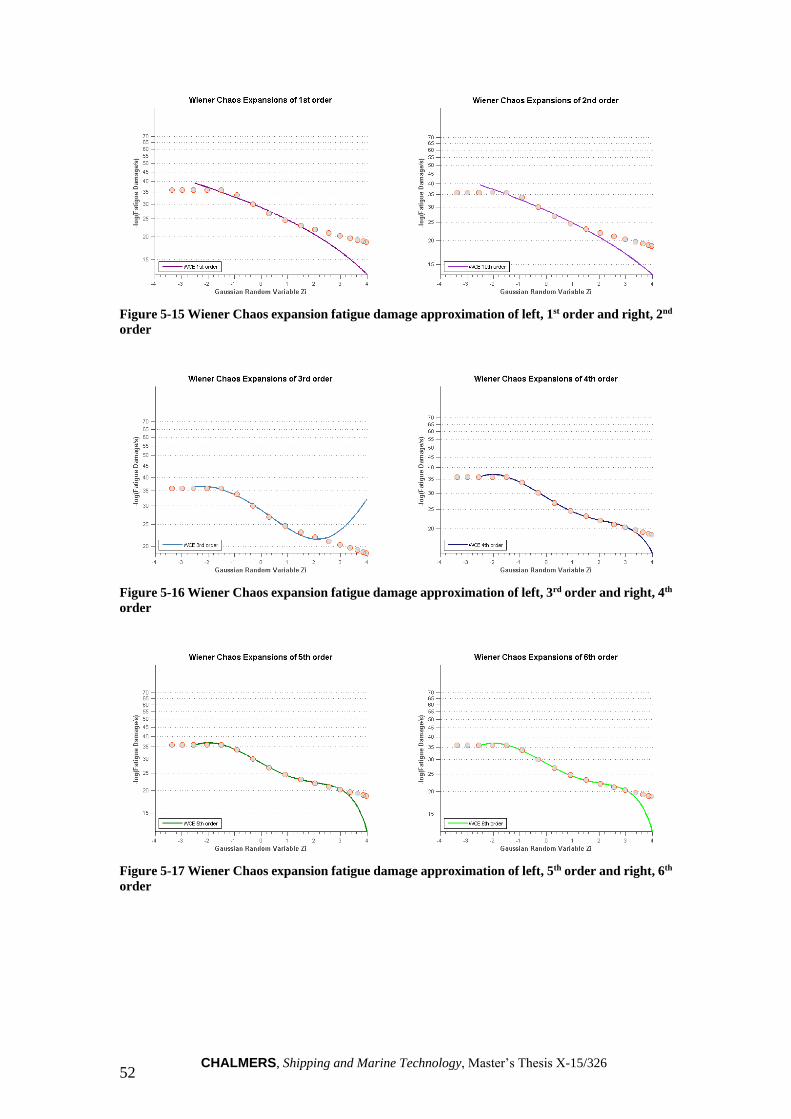
CHALMERS, Shipping and Marine Technology, Master’s Thesis X-15/326 52
Figure 5-15 Wiener Chaos expansion fatigue damage approximation of left, 1st order and right, 2nd
order
Figure 5-16 Wiener Chaos expansion fatigue damage approximation of left, 3rd order and right, 4th
order
Figure 5-17 Wiener Chaos expansion fatigue damage approximation of left, 5th order and right, 6th
order

CHALMERS, Shipping and Marine Technology, Master’s Thesis X-15/326 53
Figure 5-18 Wiener Chaos expansion fatigue damage approximation of left, 7th order and right, 8th
order
As can be observed from Figure 5-17 to Figure 5-19 the approximated fatigue damage
shows a good fit to the estimation results except for the tail where it shows an
overestimation in all cases but Wiener chaos expansion of 9th order. This is the result
of the calm sea conditions implemented in the process of obtaining Wiener chaos
expansion parameters with irregularities due to unstable dynamic equilibrium.
Figure 5-19 Wiener Chaos expansion fatigue damage approximation of left, 9th order and right,
10th order
In FiguresFigure 5-20 to Figure 5-23 result of the Hermite polynomial chaos expansion
for approximating fatigue damage is compared to spectral methods of fatigue
approximation and estimation. Fatigue damage rate calculated by direct rainflow
counting of the stress time series is used as reference to evaluate the different methods.
Here Wiener chaos expansion of 9th order is chosen to represent the approximation
method.
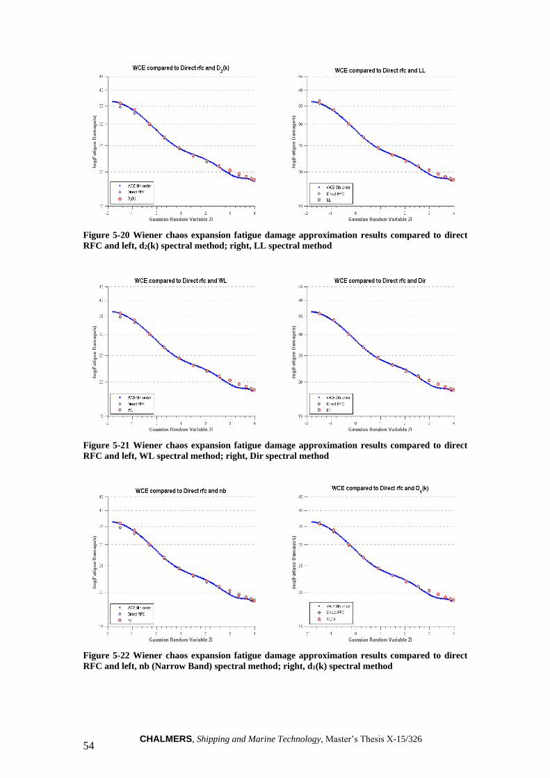
CHALMERS, Shipping and Marine Technology, Master’s Thesis X-15/326 54
Figure 5-20 Wiener chaos expansion fatigue damage approximation results compared to direct
RFC and left, d2(k) spectral method; right, LL spectral method
Figure 5-21 Wiener chaos expansion fatigue damage approximation results compared to direct
RFC and left, WL spectral method; right, Dir spectral method
Figure 5-22 Wiener chaos expansion fatigue damage approximation results compared to direct
RFC and left, nb (Narrow Band) spectral method; right, d1(k) spectral method
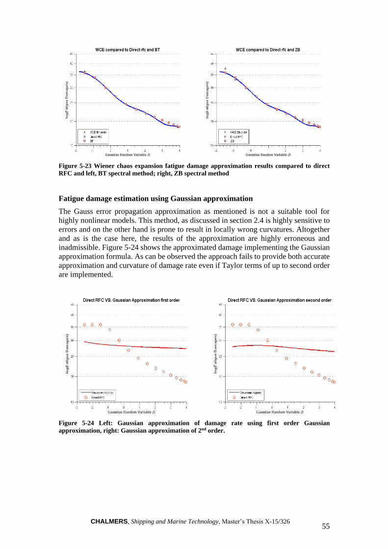
CHALMERS, Shipping and Marine Technology, Master’s Thesis X-15/326 55
Figure 5-23 Wiener chaos expansion fatigue damage approximation results compared to direct
RFC and left, BT spectral method; right, ZB spectral method
Fatigue damage estimation using Gaussian approximation
The Gauss error propagation approximation as mentioned is not a suitable tool for
highly nonlinear models. This method, as discussed in section 2.4 is highly sensitive to
errors and on the other hand is prone to result in locally wrong curvatures. Altogether
and as is the case here, the results of the approximation are highly erroneous and
inadmissible. Figure 5-24 shows the approximated damage implementing the Gaussian
approximation formula. As can be observed the approach fails to provide both accurate
approximation and curvature of damage rate even if Taylor terms of up to second order
are implemented.
Figure 5-24 Left: Gaussian approximation of damage rate using first order Gaussian
approximation, right: Gaussian approximation of 2nd order.

CHALMERS, Shipping and Marine Technology, Master’s Thesis X-15/326 56

CHALMERS, Shipping and Marine Technology, Master’s Thesis X-15/326 57
6 Conclusion and future work
Here the aim is to provide the conclusions made after the results were developed and to
suggest future steps which were limited by time during this thesis work.
As mentioned in this project to obtain the simulation results in various sea conditions
the DeepC software package was used. Unfortunately due to modelling shortcomings
and or maybe limited knowledge of application the final results of the so called calm
sea conditions seem to be erroneous. As the goal of this thesis work is to evaluate fatigue
approximation methods this erroneous force time series have an undeniable impact on
the approximated and estimated fatigue damages. In case of spectral approaches this
matter does not affect the end result as much as these sea states can simply be neglected.
But in case of the Wiener chaos expansion the fitted curve to approximated damages
shows overestimation of fatigue damage in the extreme sea states which can be the
effect of erroneous results in the calm sea conditions. Here the magnitude of errors
when implementing Gaussian approximation formula is so high that it was dismissed
as a valid method to be used in the scope of this thesis. This might have not been the
case if parameter variations were not as high as it is in the present case.
Furthermore the spectral estimation and approximation methods show very promising
results although some give highly overvalued and or underestimated results considering
fatigue damage, but in any case most provide acceptable results specifically in case of
most common sea conditions.
Based on the results the Wiener chaos expansion proves to be rather accurate in
approximating fatigue damage especially since even in erroneous sea conditions it
provides an overestimation of the damage. Altogether implementing Wiener chaos
expansion seems to be a promising method for fatigue damage approximation and a
method worth further investigations. Based on the regulations the fatigue life
estimations in a station keeping operation should be evaluated for various sea conditions
including detailed simulations based on specific wave heights, peak periods, and
environmental directions. Although other various curve fitting methods are available
the point that makes Wiener chaos expansion worthy of further study is the fact that
including more than one parameter in the method does not imply drastic complications
in regards to number of simulations. This makes The WCE an interesting approach in
comparison to other methods.
Future work
Here and in this study for sake of simplicity the standard normal variable is assumed to
be one dimensional i.e. representing the specific wave height in a Pierson-Moskowitz
wave energy spectrum. This is while the fatigue damage studies in the scope of
industrial operations is dependent on many variables to be exact the wave peak period,
other environmental conditions and headings or directions of the environment.
Approximating fatigue damage using a two parameter or more WCE would be of high
value and an interesting step forward. Another approach to the last issue could be
truncation of the approximation method which is worth looking into. Here to calculate
the parameters of the expansion a Gaussian quadrature scheme with accuracy n=20 is
implemented. This dictates 20 different simulations; it would be of value to investigate
the effect of lower accuracies on approximated fatigue damage so that if possible, the
number of simulation conditions are reduced.

CHALMERS, Shipping and Marine Technology, Master’s Thesis X-15/326 58
CHALMERS, Shipping and Marine Technology, Master’s Thesis X-15/326 59
References
ASTM. (2005). Standard Practices for Cycle Counting in Fatigue Analysis ASTM
International E1049-85.
Astrup, O. C. (2004). DeepC A White Paper. In DNV Software (Ed.): DNVS.
Atkinson, R. J., Winkworth, W. J. G., Norris, M. (1960). Behavior of Skin Fatigue
Cracks at the Corners of Windows in a Comet 1.
Benasciutti, D. (2004). Fatigue analysis of random loadings. PhD. Thesis. Ferrara.
Benasciutti, D., Tovo, R. (2007). Comparison of Spectral Methods for Fatigue Damage
Assessment in Bimodal Random Process. Paper presented at the Proceesdings
of the 9th International Conference on Structural Safety and Reliability, Rome,
Italy
Bendat, J. S. (1964). Probability functions for random reponses: Predictions of peaks,
fatigue damage and catastrophic failures. Technical report. NASA.
Bengtsson, A., Rychlik, I. (2009). Uncertainty in fatigue life prediction of structures
subject to Gaussian loads. Journal of Probabilistic Engineering Mechanics, Vol.
24, 224-235.
Brodtkorb, P. A., Johanneson, P., Lindgren, G., Rychlik, I. (2000). WAFO: A
MATLAB toolbox for analysis of random waves and loads. ISOPE 2000, Vol.
3, 343-350.
Cooley, J. W., Tukey, John W. (1965). An algorithm for the machine calculation of
complex Fourier series. Math. Comp.(19), 297-301.
Dirlik, T. (1985). Application of computer in fatigue analysis. PhD. Thesis. University
of Warwick, UK.
DNV-RP-C203 - Fatigue Design of Offshore Steel Structures (2011).
DNV-OS-E301 - Position Mooring (2013).
DNV-RP-C205 - Environmental Conditions and Environmental Loads (2014a).
DNV. (2014b). SESAM User Manual DeepC Deep water floater motion analysis.
Norway: Det Norske Veritas.
DNV.GL. (2015a). Complex multibody calculations - Simo. Retrieved 5.6, 2015, from
https://www.dnvgl.com/services/complex-multibody-calculations-simo-2311
DNV.GL. (2015b). Riser analysis - Riflex. Retrieved 5/7, 2015, from
https://www.dnvgl.com/services/riser-analysis-riflex-2312
Dowling, N. E. (2013). Mechanical Behavior of Materials, Engineering Methods for
Deformation, Fracture, and Fatigue (fourth ed.): Peaeson Education Limited.
Hou, T. Y., Luo, Wuan, Rozovskii, Boris, Zhou, Hao-Min (2006). Wiener Chaos
expansions and numerical solutions of randomly forced equations of fluid
mechanics. Journal of Computational Physics.
Jiao, G., Moan, T. (1990). Probabilistic analysis of fatigue due to Gaussian load
processes. Probabilistic Engineering Mechanics, Vol. 5 (2), 76-83.

CHALMERS, Shipping and Marine Technology, Master’s Thesis X-15/326 60
Johannessen, K., Meling, Trond Stokka, Haver, Sverre. (2002). Joint Distribution for
Wind and Waves in Northern North Sea. International Journal of Offshore and
Polar Engineering, Vol. 12(1).
Kamermans, M. P. (2011). Gaussian Quadrature Weights and Abscissae. Retrieved
5/17, 2015, from http://pomax.github.io/bezierinfo/legendre-gauss.html
Li, L., Gao, Zhen, Moan,Torgeir. (2015). Joint Distribution of Environmental
Condition at Five Europian Offshore sites for Design of Combined Wind and
Wave Energy Devices. Jornal of Offshore Mechanics and Arctic Engineering,
Vol. 137.
Lie, H. (1990). MIMOSA-2 User's Documentation MARINTEK Report No. MtT51 F
90-0358. Teondhaim, Norway.
Longuet-Higgins, M. S. (1957). The statistical analysis of a random, moving surface.
Philosophical Transactions of the Royal Society, Series A.
Lutes, L. D., Larsen, C.E. (1990). Improved spectral method for variable amplitude
fatigue prediction. Journal of Structural Engineering, Vol. 116(4), 1149-1164.
Mao, W. (2010). Fatigue Assessment and Extreme Response Prediction of Ship
Structures. Chalmers University of Technology and University of Gothenburg
Gothenburg, Sweden.
Matsuishi, M., Endo, T. . (1968). Fatigue of Metals Subjected to Varying Stress Paper
presented at the Kyushu Branch of Japan Society of Mechanics Engineering,
Fukuoka, Japan.
Milne, I. (1994). The Importance of Management of Structural Integrity. Engineering
Failure Analysis, Vol.1(n.o. 3), 171-181.
Rajesh, T., Natarajan,Kannah R. (2006). EFFECT OF TURRET LOCATION ON
DYNAMIC BEHAVIOUR OF AN INTERNAL TURRET MOORED FPSO
SYSTEM. Journal of Naval architecture and Marine Engineering.
Rankine, W. J. M. (1842). On the causes of the unexpected breakage of the journals of
railway axles, and on the means of preventing such accidents by observing the
law of continuity in their construction. Institution of Civil Engineers, Minutes
of Proceedings, 105-108.
Rayleigh, L. (1880). On resultant of a large number of vibrations of the same pitch and
arbitrary phase. Philosophical Magazine.
RIFLEX. (2012). RIFLEX - User Manual Version 4.0 rev. 0.
Rychlik, I. (1987). A new definition of the rain-flow cycle counting method
International Journal of Fatigue, Vol. 9(No. 2), 119-121.
Rychlik, I. (1993). "narrow-band" approximation for expected fatigue damage.
Probabilistic Engineering Mechanics, Vol. 8, 1-4.
Sakai, S., Okamaru, H. . (1995). On the Distribution of Rainflow Range for Gaussian
Random Processes with Bimodal PSD. JSME International Journal. Series A.
mechanics and material engineering, Vol. 38-A(4), 440-445.
Sarkar, S., Gupta, Sayan, Rychlik, Igor. (2011). Wiener chaos expansions for estimating
rain-flow fatigue damage in randomly vibrating structures with uncertain
parameters. Probabilistic Engineering Mechanics, Vol.26(2011), 387-398.

CHALMERS, Shipping and Marine Technology, Master’s Thesis X-15/326 61
SIMO. (2012a). SIMO - Theory Manual Version 4.0 rev. 1. In MARINTEK (Ed.).
Trondheim, Norway: MARINTEK.
SIMO. (2012b). SIMO - User's Manual Version 4.0 rev. 1. In MARINTEK (Ed.).
Trondheim, Norway: MARINTEK.
Tovo, R. (2002). Cycle distribution and fatigue damage under broad-band random
loading. . International Journal of Fatigue, Vol. 24, 1137-1147.
Wirsching, P. H., Light, M.C. (1980). Fatigue under wide band random stresses.
Journal of rhe Structural Division, Vol. 106(7), 593-607.
Wright, D. (2005, 04.27.2015). Fracture - some maritime examples. from
http://school.mech.uwa.edu.au/~dwright/DANotes/fracture/maritime/maritime.
html
Zhao, W. B., M. . (1992). On the probability density function of rainflow stress range
for stationary Gaussian processes. International Journal of Fatigue.

CHALMERS, Shipping and Marine Technology, Master’s Thesis X-15/326 62
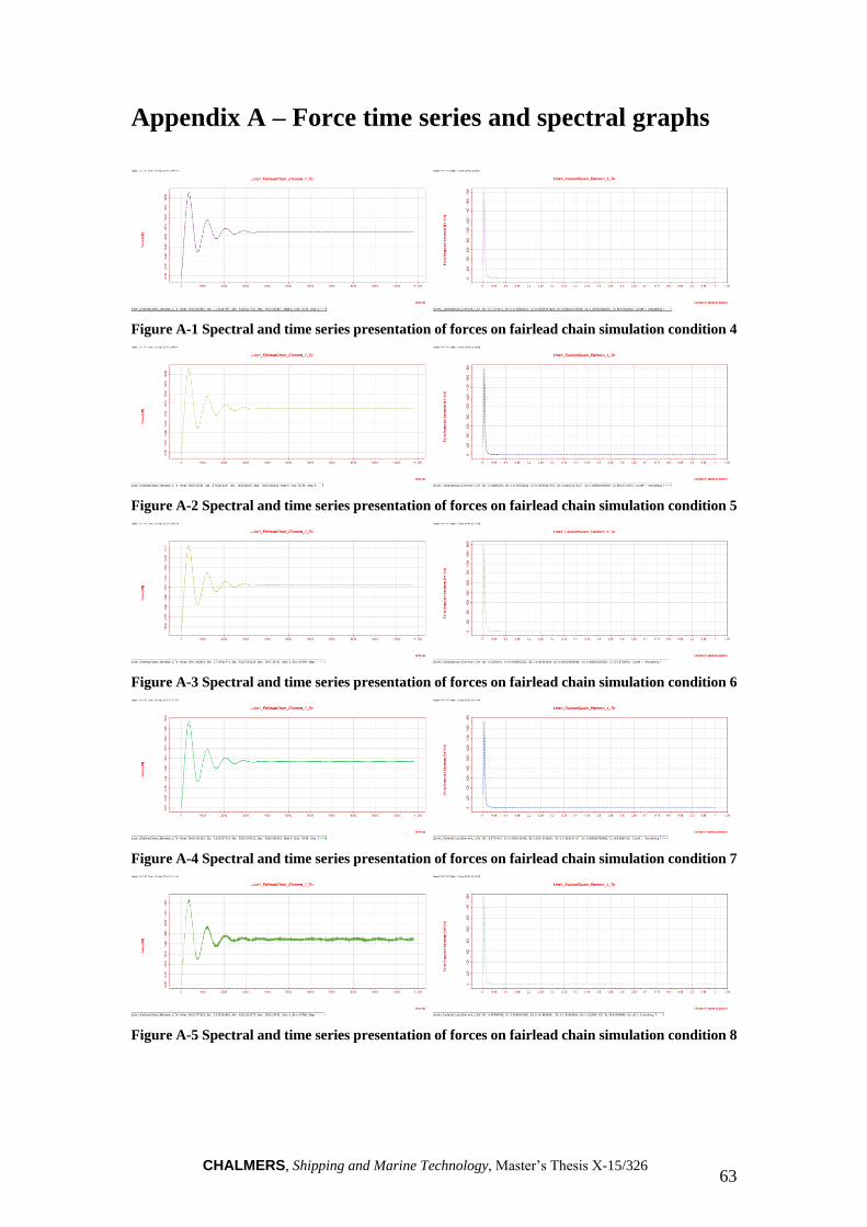
CHALMERS, Shipping and Marine Technology, Master’s Thesis X-15/326 63
Appendix A – Force time series and spectral graphs
Figure A-1 Spectral and time series presentation of forces on fairlead chain simulation condition 4
Figure A-2 Spectral and time series presentation of forces on fairlead chain simulation condition 5
Figure A-3 Spectral and time series presentation of forces on fairlead chain simulation condition 6
Figure A-4 Spectral and time series presentation of forces on fairlead chain simulation condition 7
Figure A-5 Spectral and time series presentation of forces on fairlead chain simulation condition 8

CHALMERS, Shipping and Marine Technology, Master’s Thesis X-15/326 64
Figure A-6 Spectral and time series presentation of forces on fairlead chain simulation condition
10
Figure A-7 Spectral and time series presentation of forces on fairlead chain simulation condition
11
Figure A-8 Spectral and time series presentation of forces on fairlead chain simulation condition
12
Figure A-9 Spectral and time series presentation of forces on fairlead chain simulation condition
13
Figure A-10 Spectral and time series presentation of forces on fairlead chain simulation condition
14

CHALMERS, Shipping and Marine Technology, Master’s Thesis X-15/326 65
Figure A-11 Spectral and time series presentation of forces on fairlead chain simulation condition
15
Figure A-12 Spectral and time series presentation of forces on fairlead chain simulation condition
16
Figure A-13 Spectral and time series presentation of forces on fairlead chain simulation condition
17
Figure A-14 Spectral and time series presentation of forces on fairlead chain simulation condition
18
Figure A-15 Spectral and time series presentation of forces on fairlead chain simulation condition
19

CHALMERS, Shipping and Marine Technology, Master’s Thesis X-15/326 66
Top Related