


Languages
Pages
Legal


What Will It Do For My EPS?
A Straightforward But Powerful Motive for Mergers
Gerald T. Garvey
Todd T. Milbourn
Kangzhen Xie
Date: December 20, 2013
Abstract: There is widespread evidence that bidders are more highly valued than their targets, and that both parties tend to be in temporarily high-valued industries. We find that valuation differences are also uniquely important for predicting who will be acquired and when. A firm is more likely to be a target when others in the industry could acquire them in a stock-swap merger that appears accretive to the buyer even after paying a substantial premium. The resulting measure is related to the dispersion of valuation multiples within an industry, but is grounded in a specific model of managerial behavior and is empirically much stronger than dispersion. Indeed, it is a stronger target predictor than any measure in the existing literature, including recent industry-level merger activity. Our results for bidders are less impressive. We find that a firm is more likely to be a bidder when it has more accretive targets, but unlike target prediction our effects are subsumed by existing size and valuation measures in the literature. (JEL G34, G14, G31)
________________________________
Garvey is from BlackRock, e-mail: [email protected]. Milbourn (contact author) is from the Olin Business School, Washington University in St. Louis, tel: 314-935-6392, e-mail: [email protected]. Xie is from the Sam M. Walton College of Business, the University of Arkansas, e-mail: [email protected]. We would like to thank Joshua Pierce for a very useful discussion at the 2010 FMA annual meeting. We would also like to thank Henrik Cronqvist, Jarrad Harford, Eric Hughson, Bob Marks, Harold Mulherin and Neal Stoughton for helpful comments, as well as seminar participants at the University of Texas at Dallas.

What Will It Do For My EPS?
A Straightforward But Powerful Motive for Mergers
Abstract: There is widespread evidence that bidders are more highly valued than their targets, and that both parties tend to be in temporarily high-valued industries. We find that valuation differences are also uniquely important for predicting who will be acquired and when. A firm is more likely to be a target when others in the industry could acquire them in a stock-swap merger that appears accretive to the buyer even after paying a substantial premium. The resulting measure is similar to the dispersion of valuation multiples within an industry, but is grounded in a specific model of managerial behavior and is empirically much stronger than dispersion. Indeed, it is a stronger target predictor than any measure in the existing literature, including recent industry-level merger activity. Our results for bidders are less impressive. We find that a firm is more likely to be a bidder when it has more accretive targets, but unlike target prediction our effects are subsumed by existing size and valuation measures in the literature. (JEL G34, G14, G31)

1. Introduction
It has recently been argued that acquisitions are driven by stock market valuations rather
than the synergies or managerial objectives stressed in the earlier literature (Shleifer and Vishny,
2003; Rhodes-kropf and Viswanathan, 2004; Jensen, 2005). For example, an economic shock
that differentially affects firm valuations in an industry could motivate acquisitions of some
“cheaper” firms by the more highly-valued firms. This view is buttressed by evidence that bidders
are more highly valued than their targets (Dong et al, 2006), and that both parties tend to be in
temporarily high-valued industries (Rhodes-Kropf et al, 2005).
We harness the valuation approach in a more ambitious attempt to match up and predict
bidders and targets. We append a basic “EPS bootstrap game” as described in the classic text of
Brealey et al (2007), to the seminal model of Shleifer and Vishny (2003). The outcome is an
algorithm that deems any two firms in the same two-digit SIC industry as viable candidates to
merge if by using stock at the method of payment, the putative buyer (simply the party with the
higher multiple) can increase its earnings per share (EPS) after paying the hypothetical target a
substantial premium. We also consider candidate pairs as viable if under the same conditions, the
deal would increase either the acquirer’s book or intrinsic value per share. The resulting measures
broadly resemble the dispersion of valuation multiples within an industry as used in Harford (2005),
but are grounded in a specific model of managerial behavior and empirically are much stronger
than dispersion.
While we use an exhaustive set of controls in our empirical analysis, our key findings can
be seen in a univariate comparison of variable averages for firms that then fall into one of three
categories in the subsequent year: bidder; target, and finally, the vast majority of firms that are
1

neither a bidder nor a target. For comparability across disparate scales, Figure 1 expresses all
values as z-scores; raw values are all presented in the empirical section.1
The first trio of bars conveys our main result. The number of viable bidders is far higher
for firms that are actually acquired in the next year than for firms that are either bidders or are not
involved in any M&A activity as either a buyer or a seller. The next trio, for viable targets, is
equally supportive of our model; subsequent bidders have a far greater number of accretive targets
than either of the other two categories. As bidders and targets are in both cases distinct from the
vast majority of firms that are not involved in any M&A activity in a given year, we can also
predict overall merger activity. As we show below, this also applies at the industry and market-
wide levels. We also confirm that deals predicted by our model (where the bidder has many
accretive targets and the targets many accretive bidders) tend to use stock rather than cash as the
means of payment.
Our target results are robust to controlling for other well-known variables, but our bidder
results are not. The remaining bars in Figure 1 clearly convey the reason. Size and valuation
metrics also strongly distinguish bidders from the other two categories; bidders are both larger and
more highly valued whether one uses simple book or earnings ratios or the two short-run
components of Rhodes-Kropf et al (2005)’s valuation measures. However, these measures are not
successful in distinguishing targets from the vast preponderance of firms that are neither bidders
nor targets.2 The only two measures that succeed in this dimension are the residual “long-run”
component of valuation from Rhodes-Kropf et al’s decomposition, and to a lesser extent the “wave”
1 Given our sample size, absolute z-scores above 0.3 are significantly different from zero at the 1% level. 2 This provides at least a partial explanation for why the market reaction to merger announcements is so
much larger for targets than for bidders. It is much harder to predict targets than to predict bidders so the announcement should be more of a surprise for the former (See Prabhala 1997)
2

variable capturing recent merger activity in the industry. These variables are useful but
substantially less powerful than the number of accretive buyers in identifying potential targets. In
a nutshell, it is substantially easier to distinguish likely bidders than it is to distinguish likely targets,
and our accretion metric is the strongest measure in this more difficult game. “Wave” is the single
best predictor of whether a firm will be involved in a merger as bidder or target. This is quite
logical since by construction it only flags potential hotbeds of merger activity without
distinguishing bidders and targets. Second, laying the three components of Rhodes-Kropf et al
(2005) alongside each reminds us of the key role played by their value decomposition. Long-run
V/B works in distinguishing bidders and targets because it’s the residual from two other fitted
components.
On the measurement side, we consistently find much stronger results using analyst forecast
than historical information. Specifically, we find that measuring accretion with expected future
earnings per share or a proxy for intrinsic value combining book and forecast earnings (residual
income or “RIM”) performs far better than historical earnings or simple book. Moreover, we find
strong evidence that bidders prefer targets that are attractive on both forward earnings and RIM.
This is consistent with value-maximization in that it emphasizes future rather than historical
outcomes, and combining multiple metrics makes sense given the error involved in any such
forecast. In contrast to the older literature on agency and hubris, the recent literature on valuation
differences and mergers portrays management as attempting to maximize their own shareholders’
long-term wealth in a market with substantial pricing errors. Our model is more positive than
normative along these lines; we simply posit that managers seek to increase per-share
fundamentals without strong evidence on whether or not this is in the interest of their shareholders.
3

The remainder of the paper is organized as follows. Section 2 gives a brief literature review
and develops a simple model of mergers based on the framework of Shleifer and Vishny (2003).
We then describe our approach for determining the number of viable buyers and viable targets for
each firm and the corresponding predictions. Section 3 describes our data sample and methodology.
Section 4 presents the empirical results, including the results obtained when the acquisition
premium is varied. Section 5 concludes. Appendix A contains details related to the SDC dataset,
and Appendix B contains a summary of our variable definitions.
2. Hypothesis Development
2.1 Related Literature
There is a rich literature in both theoretical and empirical camps with respect to whether
firm misvaluation drives merger activity. Closest to our work is Shleifer and Vishny (2003)
model’s where acquirers take advantage of market misvaluation by using overvalued stock as
currency to buy relatively less overvalued targets. The target benefits in the short term by getting
a premium in the deal. The acquirer benefits in the long term by getting a larger share of the
combined firm than they can get if both firms are evaluated at their long-run values.
Fuller and Jensen (2002) maintain that some CEOs engage in an earnings game by catering
to analysts with high guidance on earnings. Jensen (2005) further predicts that overvalued equity
may lead to bad acquisitions, which reduces the core values of the firms and results in poor long-
term operating performance. This approach is also consistent with our approach; in terms of the
Shleifer and Vishny (hereafter SV) model, it would be akin to managers mistakenly or carelessly
believing that the market will use the acquirer's multiple for the combined entity.
4

Rhodes-Kropf and Viswanathan (2004) (hereafter RKV) also offer a model based on
market misvaluation, but targets are not myopic as in Shleifer and Vishny (2003). Instead, the
stock values of both targets and acquirers can deviate from their long-run fundamental values.
RKV separate this stock misvaluation into a market-wide (or sector) component and a firm
component. The target CEOs cannot determine how much of this misvaluation is due to firm-
specific reasons rather than market or sector misvaluation. For two firms in the economy (or in the
same section), the market-wide (or sector) component in misvaluation is common to both the
acquiring and the target firms. The target CEO correctly adjusts downward the stock offer received
from the acquirer, but he still accepts the offer because he overestimates the merger synergies
owing to the common misvaluation of the market or sector.
Dong, Hirshleifer, Richardson and Teoh (2006) test both misvaluation and Q theories of
mergers. They use price-to-book to proxy for a firm’s growth opportunities in Q theory and also
as a proxy for misvaluation. They also use price-to-value based on Lee et al (1999) as another
proxy for misvaluation. They find both that measures are important and further find that the
evidence for the Q hypothesis is stronger in the pre-1990s period than in the 1990-2000 period,
while the evidence for misvaluation is stronger in the 1990-2000 period. The key difference from
our paper is that their tests focus on deals that actually take place, while we include nearly all firms
for which there is publicly-available data and focus on the arguably tougher issue of predicting a
priori which firms ultimately become acquirers or targets.
Rhodes-Kropf et al. (2005) test the RKV and Shleifer and Vishny (2003) models using an
empirical valuation model that includes book values, net income and leverage to decompose the
market value mispricing into three components. The three components of this decomposition are
a firm-specific error, a sector mispricing error and a long-run mispricing error. They find that both
5
targets and acquirers have a higher market-to-book (M/B) relative to non-merger firms, and high
M/B targets are bought by even higher M/B acquirers. The firm-specific error is higher for
acquirers than targets in the overall merger sample and for the stock-financed sample. However,
they also find that low long-run, value-to-book firms acquire high long-run, value-to-book targets.
This is puzzling given existing theory, especially Q theory which argues that firms with high
growth opportunities should buy firms with low growth opportunities. They argue that the
contradicting results of high M/B buying low M/B and long-run value-to-book buying high long-
run value-to-book call for some form of market inefficiency and informational asymmetry. The
empirical work of Rhodes-Kropf et al (2005) explains a significant amount of overall merger
activity, medium of exhange, and bidder identification, and we blend their measures into all of our
empirical tests.3
2.2 A Simple Model and resulting Hypotheses
We develop a simple model of mergers following Shleifer and Vishny (2003) (hereafter
SV) and then derive two new, empirically-testable predictions. As in SV, consider a representative
3 There are other papers focusing on tests of whether the acquisitions benefit or hurt the shareholders of the acquiring firms. Ang and Cheng (2006) use a similar P/B and P/V approach and have findings analogous to those in Dong et al (2006). Further, they show that the shareholders of acquirers in stock mergers are as well off as, if not better off than, the shareholders of similarly overvalued non-acquiring firms. Moeller et al (2005) find that negative bidder returns from 1998 to 2001 are driven by a few deals in which the bidders with extremely high values suffer huge losses after merger. They find that such firms have high q's and high market-to-book ratios. Thus, this provides support for Fuller and Jensen’s (2002) claim that managers of high valuation firms make poor acquisitions. However, the negative returns can also be due to the market's adjustment of the true stand-alone values of such firms. Song (2007) uses the trading of insiders as an indication of the overvaluation of their firms. She finds a strong relation between the insider selling prior to the merger announcement and long-run post-acquisition performance in the “hot market” period of 1997-2000. Bouwman et al (2009) find that acquisitions in high valuation periods generate a significantly lower long-term abnormal return for the buyers and suffer a significantly lower long-run operating performance. However, they show that market timing is not likely an explanation for the underperformance of acquirers in high valuation market. Fu et al (2009) investigate whether acquirer shareholders benefit from acquisitions driven by equity overvaluation. They sort acquisitions by relative overvaluation before the announcement. Their findings support Jensen's (2005) hypothesis that equity overvaluation generates substantial agency costs for shareholders. Bi and Gregory (2009) use UK data and find more support for the market misvaluation hypothesis than the Q theory, however they cannot comprehensively reject the Q theory explanation.
6
merger pair, denoted firm 0 and firm 1. Firm 0 (firm 1) has K0 (K1) units of capital and the stock
price is a multiple Q0 (Q1) of the capital. Assume without loss of generality that
Q1 > Q0,
so firm 1 is the prospective acquirer and firm 0 the prospective target. The key parameter in SV is
s, the synergy that the market attaches to the combined entity. Specifically, the market value of the
combined entity is
1 0 1 0] [ ][ (1 )K K sQ s Q+ × + − .
SV refer to this as the short-term market value, so that s can contain pricing errors. In the
baseline case where there are no synergies and the market is efficient, 1
1 0
KK
sK
=+
. The target firm
shareholders and management are assumed able to cash out immediately after the deal closes, so
they are not concerned with longer-term value. Hence, what matters for the viability of the
combination is the bidding firm’s view of s.
The second component of SV’s model is the longer-term return to the two entities. The key
component of this analysis for our purposes (predicting the incidence of mergers) is the fact that
the bidder must pay a non-zero premium given by a percent of target value. Finally, assume without
loss of generality that both firms have a single share outstanding and that the acquirer issues an
additional m shares to the target. We now have two conditions for a merger pair to be viable. First,
the bidder must provide enough shares, m, to cover the required premium of Π:
1 0 1 0 0 0m
1 m(sQ (1 s)Q )(K K ) Q K (1 ).
++ − + = +∏ (1)
Second, the bidder must not expect to lose market value from the bid:
7

1 0 1 0 1 11
1 m(sQ (1 s)Q )(K K ) Q K .
++ − + ≥ (2)
Conditions (1) and (2) are satisfied so long as:
0 0
1 0 1
1
0
Q Ks( K K ) K
QQ− ∏
>+ −
. (3)
The problem with taking this to the data is that we cannot observe the bidder’s beliefs about s.
Two extreme cases are instructive. In an efficient market and management that doesn’t believe in
synergy (i.e., the case where 1
1 0
Ks )K K
=+
, then the two conditions above can never be satisfied
for any Π > 0. This simply says that the bidder cannot offer a premium if there is no gain to the
merger, efficiency-based or otherwise. At the other extreme, if s = 1 (the bidder at least believes
the market will apply her higher multiple to the target’s assets), then all that is required is for the
bidder’s multiple to exceed that of the target by the premium. This is a straightforward, if extreme,
bootstrapping result. It’s useful for expositional purposes, but taking it to the real-world data
requires us to consider (at least) three issues.
First, for most reasonable premia, the range of multiples in broadly-defined industries
implies that many firms have multiple viable buyers; this implies an unconditional likelihood of a
takeover at least an order of magnitude greater than what we observe in the data. A simple way to
accommodate this fact is to posit that most potential bidders, say a fraction X of the population, do
not believe in the bootstrap game (that is, they believe in an s value closer to 1
1 0
KK K+
than to one).
Since only one viable bidder is required for the firm to be taken over, if we denote the number of
firms that satisfy conditions (1) and (2) by n, a potential target is taken over with probability
8

n1 X− . While we do not actually know X, this observation suggests we should apply a concave
transformation to the number of viable bidders when we come to our empirical tests.4
Secondly, relative size does not matter, because when s = 1 even a small bidder can apply
her multiple to a big target. This may seem counterintuitive, but Harford (1999) surprisingly finds
that targets are not, on average, small firms and we confirm this basic result in our data. To further
investigate the idea, in robustness tests we add the requirement that the bidder’s assets be greater
than those of the target 1 0(K K )> and our results hold up.
Finally, we have thus far adopted the Shleifer-Vishny modeling assumption that
differences in multiples are primarily due to mispricing, rather than appropriate valuation of
differential risks or cashflow expectations (at least, we have done so in the s = 1 case). Much of
the subsequent empirical literature (Dong et al 2004, Rhodes-Kropf et al 2005) attempts to specify
valuation models in order to isolate mispricing. Our approach hinges more on bidder behavior and
beliefs than any specific pricing model. For the target, the deal is acceptable simply if it offers a
sufficient premium. For the buyer, so long as the deal can increase its per share value (either EPS,
Book Value, or Intrinsic Value), the deal is viable. We then argue that the likelihood of a merger
is related to the number of viable buyers or targets. For a firm to sell itself, the possibility for it to
find a buyer that is able to pay it a desired premium increases with the number of viable buyers.
The more viable buyers, the larger the chance that at least one buyer is able to pay target’s desired
premium. In sum, we have:
4 This is particularly the case if we were to endogenize the required premium; it is likely to increase in the number of viable bidders and accentuate the diminishing-returns effect.
9

Hypothesis 1 (H1):
The likelihood of a firm being a target is positively related to the number of viable buyers.
Since we argue that merger activities are driven by relative misvaluation, which is captured by our
estimates of viable buyers and targets based on stock financed deals, we have the following
additional prediction.
Hypothesis 2 (H2):
The likelihood of the use of stock as method of payment is positively related to the number
of viable buyers and viable targets.
A priori, we have less confidence in H2 than H1. From the work of Boone and Mulherin (2007)
on the process of selling a target, it is quite likely that the presence of viable stock-financed buyers
may put a firm “in play”, but the eventual successful buyer may use a significant amount of cash.
This is particularly likely if there are many potential bidders.
3. Sample and Empirical Methodology
We begin by detailing our data and sample selection, then define our variables of interest
and delineate our controls. We close the section by summarizing descriptive statistics, including
some univariate results on our first empirical prediction that the likelihood of a firm being a target
is positively related to the number of viable buyers.
3.1 Data
We begin with all firms in the Compustat universe, but also require merger data which are
drawn from SDC Platinum dataset. We download all deals with domestic targets from the SDC
database from 1981 to 2012. The search includes all transactions that take the form of “Merger,
10

“Acquisition of Majority Interest”, “Acquisition” or “Acquisition of Assets”. We only consider
deals in which the acquiror is acquiring an interest of 50% or over in a target. We do not include
other types of deals because we are only interested in cases where the buyers achieve a controlling
interest and can integrate (or consolidate) the targets’ financials into their own and for details of
our sample composition. See Appendix A for the definitions from SDC and the details or our
sample construction.
To calculate forecasted EPS-based and intrinsic value-based numbers of viable buyers and
targets, we also use I/B/E/S earnings annual forecast data. We use the one year (fiscal) average
EPS forecast in I/B/E/S as the forecasted EPS for the firms in the year. In order to use the residual
income model to calculate a firm’s intrinsic value, we also use I/B/E/S year two and year three
(when available) EPS forecasts, along with the long-term growth rate forecast.
3.2 Empirical Specification and Key variable
We estimate the following Probit regression model for merger likelihood:
𝑦𝑦𝑖𝑖,𝑡𝑡 = 𝑓𝑓(𝛼𝛼 + 𝛽𝛽1𝑉𝑉𝑖𝑖,𝑡𝑡−1 + 𝛽𝛽2𝑋𝑋𝑖𝑖,𝑡𝑡−1 + 𝛽𝛽3𝑍𝑍𝑡𝑡 + 𝛽𝛽4𝑊𝑊𝑡𝑡−1 + 𝜇𝜇𝑡𝑡 + 𝜈𝜈𝑗𝑗) (4)
where the subscript i refers to firm i, the subscript t refers to time in years, the subscript j refers to
industry, µt refers to time fixed effects and νj refers to industry fixed effects. The dependent
variable y is an indicator variable for a merger. In the regression of target likelihood, y will be
equal to 1 if firm i is a target in year t and 0 otherwise. The corresponding V is the number of viable
buyers for firm i at year t-1. X’s are the control variables including firm i's size, market to book
ratio, leverage and price to earnings ratio. Z is the level and standard deviation of the related key
variable within the industry at year t. W is the number of takeover that took place in firm i's industry
j. In the regression of the likelihood of using stock as the method of payment, y is defined as an
11

indicator variable that takes the value of 1 if the deal uses only stock as the method of payment
and 0 otherwise.
3.3 Test Variables
To compute the number of viable buyers for each firm, we assume that any potential buyer
will pay for the target with its own equity. For a given firm in each year, we compute the number
of firms that are able to make an equity-financed deal that is earnings per share accretive and pays
a 20% acquisition premium to the target. For example, we identify firm B as a viable buyer for
firm A if firm B uses its stock to pay a 20% premium for firm A’s equity (in market value terms)
and the resulting earnings per share of firm B increases after absorbing firm A. We denote the
number of viable buyers based on EPS as Accretive Bidders. Figure 2 shows that the median
number of EPS Accretive Bidders per firm moves closely with the total number of public firms
being taken over each year. It also show a weaker relationship using the level of the market or the
dispersion of valuation multiples. In Panel A of Table 1, we run a simple multivariate test without
any controls to highlight the same message as Figure 2. Namely, that our measure of the number
of viable targets available goes a long way to explain the level of takeover activity year by year.
Below we show that this result holds up in more refined tests.
We run an analogous exercise using book values, and denote a deal as book value accretive
if firm B's book value per share increases after acquiring firm A via an equity-financed deal paying
a 20% premium. We denote the number of such viable buyers for each potential target firm as
Book Bidders, and the number of viable targets for each potential buyer as Book Targets.5 The
20% premium hurdle is clearly somewhat arbitrary and we conduct sensitivity analysis as well.
5 We exclude firms with negative book values of equity since it's difficult to interpret their economic meaning. We'll apply the same condition below when using the screen that identifies only deals that increase intrinsic value.
12

To gauge accretion in EPS or intrinsic value, we turn to the I/B/E/S data set for earnings
forecasts. We use the forecasted earnings from I/B/E/S and the mean of analysts’ EPS forecast to
proxy for the expected earnings in each firm. I/B/E/S typically provides annual earnings forecasts
out two years into the future. For the EPS-based viability measure, we only use the next year’s
forecast. But for the intrinsic value-based viability measure, we rely on the first two years' forecast
and the estimated rate of long-term growth. I/B/E/S updates analysts’ forecasts every month. Since
we are doing the estimation on a yearly basis, we use only one month’s forecast. We choose the
month when the forecasted date becomes the one year forecast for the first time. This usually
happens when a firm announces its annual report and the analysts start to shift their forecast to the
following year. Thus, it should capture the new information available in the beginning of this fiscal
year. We exclude negative earnings and hence have 156,759 firm-year observations for our
computation.
We follow mostly the method described in Dong et al (2006) to estimate a firm’s intrinsic
value from the residual income model (RIM). We exclude firms with negative book values per
share and firms when the dividend payout ratio is greater than 1. Since our sample includes all
non-merger firms and is much bigger than Dong et al (2006)’s paper, we adopt the additional
criteria of Frankel and Lee (1998) who examine the predictive power of the residual income model
for stock returns in a large sample. They argue that some firms have extremely high ROEs due to
low book equity value, and that firms with low stock prices have unstable B/P ratios and poor
market liquidity. Following their criteria, we further exclude firms with stock prices less than $1
per share in the year and further exclude firms if any of current ROE or future ROEs of one year,
two years and three years out are greater than 1. We exclude firms with negative intrinsic values.
This leaves us with a sizeable sample of 125,437 firm-years to compute the number of viable
13

buyers (targets) based on intrinsic value. However, this leaves us with a slightly smaller sample in
computing viable intrinsic value buyers and targets than we had when identifying the analogous
measures using EPS and book values. Ultimately, we denote the number of viable buyers for each
firm as RIM Bidders, and the number of viable targets for each firm as RIM Targets.
3.4 Control variables
To isolate and affirm our paper’s intended contribution, we use an exhaustive range of
controls from the existing merger prediction literature. Past studies (Hasbrouck, 1985; Palepu,
1986; Mikkelson and Partch, 1989) show that the likelihood of being a target is negatively related
to the size of the firm. We use various size measures as robustness checks, but settle on log of
assets for the results reported here. Harford (1999) shows that the stock price to earnings ratio is
positively related to the likelihood of being a target, so we also control for it. Since Cremers et al
(2008) find that leverage has a positive and significant effect on being a takeover target, we also
include leverage measured as the book value of debt divided by total assets as a control. Finally,
as our paper is most closely related to misvaluation paper by Rhodes-Kropf et al (2005), we adopt
their measures as our main control variables. Following their method, we fist decompose the
market-to-book ratio into three components, including firm-specific errors, industry time series
errors, and long run value-to-book errors. We then verify that our decomposition method obtains
similar results as those reported in the Table 9 of their paper.6 Lastly, we use the same set of firm
6 Past research has also used a host of alternative valuation metrics. Hasbrouck (1985) argues that low Market/book values can proxy for management incompetence and low cost resources for acquirers. Cremers et al (2009) finds that a firm's q is negatively related to the probability of being a target. They also find that ROA (return on assets) is negatively related to the likelihood of being a target, so we control for the ratio of net income before extraordinary items and discontinued operations to total assets. One could also include liquidity as a control variable as in Hasbrouck (1985) because it is easier for a bidder to secure a toehold in a more liquid target. In unreported tests, we add the above variables as controls, and their inclusion of these variables doesn't change any of our primary results. However, since the Rhodes-Kropf et al (2005)'s valuation decomposition measures overlap most of these valuation metrics, in the paper we don’t include them.
14

financial variables in the regressions related to the likelihood of being an acquirer as we expect
such variables should have opposite effects. We winsorize the ratios at the 1% level.
Next, we sort the data by two-digit SIC code and calendar year. Following the merger wave
literature, we compute Num_Takeover as the total number of takeovers in the industry in the year.
We also include year and industry fixed effects and cluster the standard errors at the industry level.
It is generally agreed that mergers happen more frequently in booming markets as highlighted in
Figure 2. We want to be sure that our results are not caused simply by shocks to the entire economy
or just some industries, and we also wish to be sure that we are not picking up any year effect. An
economic shock will cause overall stock price movements in the entire economy or the industry,
but we are more interested in how the relative misvaluation differences caused by the shock relate
to observed merger activities.
To make sure that our results are not driven by any industry change, we also include as
controls the industry dispersion (standard deviation and interdecile range) of all the valuation
metrics we consider (price-to-earnings, price-to-book and price-to-intrinsic-value). Buttressing
this claim, Figure 2 illustrates the positive relation between the number of deals and the market-
to-book (i.e. price-to-book) dispersion each year. Unlike dispersion statistics, the number of viable
buyers is related to the sheer number of firms in the industry. Hence, we include the number of
firms in the industry as an additional control.
3.5 Summary Statistics
We first present the summary statistics of our key variables in Panel B of Table 1, noting
that these were the data underlying Figure 1. Here, focusing on lagged values of each, Acquirer
Sample includes all firms that were an acquirer in a particular year, Target Sample includes all
15
firms that were a target in a particular year, and Non-Merger Sample includes the set of firms not
involving in a merger activity. From Panel B, we can see that the average number of viable bidders
(measured either as lagged values of Accretive Bidders, Book Bidders, or RIM Bidders) in the
target sample is significantly larger than that in the other two non-target samples. For instance,
firms in the target sample have a median of nearly 83 potential buyers (Lagged Accretive Bidders),
whereas those in the Non-Merger sample have just 50. Similarly, we find that the number of viable
targets in the acquirer sample is significantly larger than that in the other two non-acquirer samples.
Hence, our estimates of the number of viable buyers and viable targets have the potential to explain
the likelihood of a firm actually being a target or an acquirer. The mean differences are all
significant at the 1% level.7 Observe that the means and medians of viable buyers (and viable
targets) are quite different. We find that the distribution of viable buyers (and viable targets) is
highly right-skewed. Hence, following Aggarwal and Samwick (1999), we use the empirical
cumulative density function (CDF) to normalize the independent variables and run our regressions
with these transformed variables.8
Using the observed probability of a takeover for the whole sample (3.87%), and the median
number of EPS buyers for the whole sample (52), we can calculate the probability (i.e., the fraction
of the bidder population) X of not believing in the bootstrap game based on the formula $1 - X52 =
3.87%. If we apply this number with the median number of EPS buyers (83) for the target sample,
7 Due to the increased restrictions in sample selection, the number of observations in the target sample using the intrinsic value based measure (RIM Bidders and RIM Targets) are approximately one fourth lower than those in either the EPS or Book based measures.
8 In unreported results, we also use the natural log of the number of viable buyers and viable targets and obtain similar regression results as with our CDF transformed variables.
16

we obtain a probability for a firm being a target that increases to 6.11%, which is very close to the
marginal effect we find for the EPS buyer viable in the regression of Table 2.9
In Panel C of Table 1, we report the lagged means and medians of our control variables.
Differences between the target sample and the non-merger sample among the control variables are
not obvious except in the more dramatic differences between the number of takeovers by industry
(i.e., the merger wave variable) and in the number of firms in the industry. The mean differences
between the acquirer sample and non-merger sample are mostly significant, and almost always at
the 1% level. Most of the differences are in accordance with the literature. For example, the size
and the price to earnings ratio for the acquirer sample are larger than those of the non-acquirer
samples. Also, the price to earnings ratio in the acquirer sample is much larger than that found in
the non-acquirer samples. Hence, these variables are arguably relevant controls for our tests.
Echoing what we show in the Figure 1, such differences have already provided much information
to a priori identifying a likely acquirer (a lá Rhodes-Kropf et al (2005)), and hence the viable target
variable does not stand out in predicting the acquirer.
The correlations between our test variables are contained in Panel D. The viable buyers
variables are correlated among themselves at ranges between 60-80%, suggesting that our
measures of viability are picking up different facets of managerial behavior. The viable target
variables we construct are also correlated amongst themselves, albeit at lower levels. The
correlations between our measures of viable buyers and targets are very low, and otherwise, few
surprises are revealed here among our remaining controls.
9 Observe that are estimated coefficient for the marginal effect of the number Accretive Bidders ranges from 5.37% to 5.8% in columns 1-3 of Table 2.
17
An important observation from Panel D of Table 1 is the high correlations between the
number of takeovers by industry and each of our measures of the number of viable bidders and
targets. One reason is that while our model is focused on individual firms as targets, we use
industry to restrict our search for potential buyers. Results are not overly sensitive to our choice of
industry definition, and we also see an appealing ability to predict mergers at the industry as well
as firm level. Panel E delineates the correlations among the merger rate and median number of
each of our measures of viable bidders per firm, by industry. In the first table, we display the
median correlations across industry. The Spearman correlations are between 0.21 and 0.23 and the
Pearson correlations are between 0.28 and 0.35. Since using the industry median may not capture
the dynamics of merger activities, in the second table of Panel E, we calculate the correlation for
the median number of viable buyers and the merger rate for each industry, each year. The
Spearman correlations are quite high at around 0.36, and the Pearson correlation drops a bit to
about 0.14. Apparently, our methodology does a good job identifying industries that are likely to
be overall hotbeds of activity. By construction, the “merger” wave approach cannot do that as it
does not make a prediction until after actual mergers have been observed.
Moving to the time-series of mergers in some of the most active industries, we see that our
measures and the merger wave variables tell a similar story, with ours being more of a leading
indicator. Two industries in our sample – Depository Institutions and Business Services – have the
highest number of total deals. Figures 3 and 4 show how the number of viable bidders is related to
the incidence of subsequent deals. We notice that the number of firms in the industry for both
industries does vary a lot over years. Taken together with the collection of facts that the number
of viable bidders and targets and the number of firms in the industry in the merger samples is larger
18

than that in the non-merger sample and that the two numbers are highly correlated, we should also
include the number of firms in the industry as a control variable in our tests.
4 Main Empirical Results
With the data in hand, we can take up our primary tests to confirm that the patterns we
identify in Figure 1 and Panel A of Table 1 obtain a richer empirical setting.
4.1 Predicting Takeover Targets Based on the Number of Viable Buyers
We now turn to our test of H1 that predicts that the likelihood of being a takeover target is
increasing in the number of viable bidding firms. In the purest test of the EPS bootstrap game,
Table 2 begins the analysis with our proxy for the number of viable buyers based on whether a
deal is EPS accretive to the buyer, with the results contained in columns 1-3. The dependent
variable is a dummy which equals 1 if the firm is a takeover target and 0 otherwise. We use the
CDF transformation of independent variables in the regressions so all coefficients are directly
comparable. We run a baseline regression in column 1 that controls for the standard deviation of
the potential target’s industry P/E ratio, replacing it with interdecile range between the PE of the
firm at the 90th percentile and that of the 10th percentile in the second column, and in the third
column we rely on the three Rhodes-Kropf et al (2005) valuation measures. In strong support of
our primary hypothesis, observe that the estimated coefficients for our viable buyer measure
(Accretive Bidders) in all three regressions are positive and significant at the 1% level.10
While these results are supportive, an examination of the marginal effects of the probit
regressions truly help to underscore the univariate findings. For a firm with average attributes
10 We see that the estimated coefficients for the controls on industry valuation dispersion in columns 1 and 2 are slightly negative and not significant.
19
across the board, including the number of viable buyers, the unconditional probability of being a
target is 3.4%. In column 3, we see that the coefficient for the variable Accretive Bidders in this
marginal regression is 0.058. Hence, if the number of viable buyers goes up from the median (i.e.,
the median of the CDF transformed variable) level to the maximum, the probability of being a
target increases to 3.4% + (0.5 × 5.8%) = 6.3%, an increase of 85%. The magnitude of the
coefficient on the variable Accretive Bidders is substantially larger than any of the control variables.
The number of takeovers in a firm’s industry in the previous year marginally increases the firm’s
likelihood of being a target and is generally an important variable. A firm’s leverage is negatively
related to the likelihood of being a target, but are not significant. The number of firms in the
industry of the firm seems to decrease the probability of being target, while the price to earnings
ratio slightly increases it. The firm-specific error based on Rhodes-Kropf et al (2005)
decomposition method increases the likelihood of being a target, that is, when a firm’s is
overvalued due to pricing error of its own characteristics, it is also more likely to be taken over.
Also, when a firm has higher long run value to book deviation, it is less likely to be a takeover
target. These latter valuation controls behave essentially as they did in the authors’ original work,
as would be naturally expected.
The effect of firm size on the likelihood of being a takeover target requires some further
explanation. Most of the earlier literature agrees that small firms are more likely to be taken over.
However, Harford (1999) uses the log value of the target’s assets as proxy for size and finds that
the coefficient is not significant in the prediction of merger targets. Our results are consistent with
Harford’s, but to further investigate the issue of size and ensure it has no effect on our main results
of interest, we also split the sample according to firm size. In unreported results, we find that the
coefficient for size is negative in the sub-sample of firms above the median size and positive in
20

the sub-sample of firms below the median size, with both significant at the 1% level. This finding
points to a nonlinear relationship between size and the likelihood of being a target. Since the effect
of size on merger activity is not the primary issue in our paper, we simply add the square of the
target firm’s size in the regression to control for this nonlinear relationship. Under this
specification, the sign of size becomes insignificant across all columns in Table 2.
With our EPS bootstrap results strongly in hand, next we present our tests on whether the
likelihood of being a target is related to the number of viable buyers based on book value and
intrinsic value, and report the results in columns 4 and 5 in Table 2. From column 4, we find that
the variable Book Bidders is positively associated with the probability of being a takeover target,
and is significant at the 1% level. However, the magnitude of the coefficient is only 0.016, roughly
a third of that of Accretive Bidders. In column 5, we then test whether our measure of viable buyers
based on intrinsic value (RIM Bidders) is related to the likelihood of being a target. We find that
our viable buyer variable, RIM Bidders, is positively related to the likelihood of being a target with
a coefficient of 0.034 and is significant at the 1% level. Hence, if the number of RIM Bidders
goes up from the median level to the maximum, the probability of being a target increases by 1.7%
in absolute terms, which is a fairly significant increase of 50% from the predicted probability of
3.4% at the mean. Hence, we believe that our estimated coefficients have significant economic
meaning.
Due to the increased restrictions on the sample selection owing to data availability, the
number of observations in the analysis based on the intrinsic value-based variable is lower than
the EPS and Book based variables, so some caution is warranted in contrasting these with the
earlier results contained in previous columns. That said, while some observations are lost, we
believe that by using a valuation model, we are better able to distinguish between a market-driven
21
story (where rational managers take advantage of an irrational market) and an agency story (where
managers make mistakes or empire build, and ultimately destroy shareholder value). A valuation
model helps us reduce errors in pricing the targets by combining both book value and earnings into
a single metric in a theoretically coherently way. If the “rational managers-irrational markets”
story is true, then after removing errors in our measure of viable buyers (and targets), we should
observe an increase in our estimated coefficients. If we see the opposite, then it’s most likely driven
by managerial errors (or agency problems) and not market mis-valuation.
In column 6, we estimate the model using all three of our measures. The impact of Accretive
Bidders drops slightly, but still with a coefficient of 0.042, whereas the estimated coefficient on
Book Bidders is only 0.09 (significant at 10% level) and that of RIM Bidders is only 0.10
(significant at 5% level). Hence, the number of EPS-based viable buyers in a potential target firm’s
industry appears to have the most important effect on the likelihood of being a target. However,
since the EPS based viable bidders and RIM value-based viable bidders are highly correlated, the
effect arguably may still be driven by a value-increasing motivation on the part of acquiring
managers.
Overall, the evidence presented in Table 2 provides strong support for Hypothesis 1 that
when a firm has more viable buyers, it is more likely to be acquired. Importantly, our measures
stand up to not only the inclusion of standard controls, but also those of Rhodes-Kropf et al (2005)
and Harford (2005).
4.2 Predicting Acquirers Based on the Number of Viable Targets
We now turn our model to the empirical task of predicting likely bidders. In Table 3, we
report the results of our regression using Accretive Targets. Here, we estimate a coefficient of
22

0.032, significant at the 1% level in columns 1 and 2, suggesting that the likelihood of being a
buyer is positively affected by the number of available viable targets. However, once we add other
control variables meant to capture the misvaluation effects, including the price to earnings ratio
(i.e. P/FE), it becomes slightly negative and no longer significant, while the P/FE ratio has
reasonably strong predicting power. Clearly, firms with high price earnings ratios are more likely
to be an acquirer, and this effect subsumes our measure’s predictive effect.11 Lastly, in column 5
we add the three value measures of Rhodes-Kropf et al (2005), revealing where their measures
really shine, namely in this specific task of predicting likely acquirers. Here we see that the firm-
specific error and the industry time series error both have positive coefficients of around 0.01, with
significance levels of 5%. This is much in accordance with the findings in Rhode-Kropf et al
(2005) which show that firms whose valuation multiples are temporarily elevated above the normal
and firms in industries with temporarily high valuations are more likely to be acquirers. Also, the
long run value to book error has a quite high coefficient of 0.026, with a significance level at 1%.
This actually supports the traditional q theory. The merger wave variable, as proxied by the number
of takeovers in the industry, has a positive estimated coefficient. Clearly, one is much more
successful in predicting a potential acquirer than to identify a potential target with the misvaluation
variables from the existing literature.12
4.3 Predicting Merger Activity at Firm and Industry Levels
In Table 4, we provide the results of our model’s ability to predict overall merger activity.
We set a dummy variable equal to one if the firm is either a takeover target or a buyer, and zero
otherwise. Observe that the estimated coefficients of both the number of Accretive Bidders and
11 In column 4, we also control again for interdecile dispersion of price to earnings and find a similar result. 12 The results of Book Targets and RIM Targets are quite similar, hence we don’t report the results of
regressions here.
23

Accretive Targets variables are both positive and significant at the 1% level. Turning to the
valuation measures of Rhodes-Kropf et al (2005), we see that our estimated coefficients are similar
to theirs, but not identical. This likely because as we have a longer sample period and use a finer
industry partition than they do. Thus, similar to the findings in their Table 9, our measures of the
number of viable bidders and targets have incremental power to predict merger intensities at the
firm level.
Next, we investigate whether our measures of viable bidders and targets also predict merger
waves at the industry level, akin to the results found in Table 10 of Rhodes-Kropf et al (2005).
We define the level of the industry merger wave as the number of merger announcements in each
industry every year. Our model’s key predictive variable is the average number of Accretive
Bidders in each industry every year (i.e., Ind Average Accretive Bidders). We also include several
control variables, such as the number of firms in the industry each year and the Rhodes-Kropf et
al (2005) measures. We use the lag values in all regressions, and control for both year and industry
fixed effects. Estimates from our panel regressions are reported in Table 5.
In column 1, we find that our key variable of interest, namely Ind Average Accretive
Bidders, has strong predictive power. In column 2, we confirm that part of the effect is due to the
sheer number of firms in the industry. As an illustrative example, Figure 3 reveals the fact that a
large number of mutual banks went public in the early 1990s, driving more merger activity. In
columns 3 to 6, we include sequentially the Industry Average Market to Book Ratio, the Total
Number of Mergers in the previous year, the Total Number of Mergers in the entire industry, and
then both of these latter counts as control variables. Consistently across all specifications, the
estimated coefficient on the number of Accretive Bidders is always positive and significant at 1%
level. In columns 7 to 10, we include the Rhodes-Kropf et al (2005) measures of Industry Average
24

Time Series Error and Industry Average Long-run Value to Book Ratio as controls (see their Table
10 for detail of their variables), and again our primary variable still has strong and significant
ability to predict industry-level merger intensity alongside theirs.
4.4 Predicting the Medium of Exchange
We now turn our attention to a test of our second hypothesis, namely that the numbers of
viable buyers and targets are related to the use of stock as the medium of exchange in the
acquisition. We run probit regressions that include year and industry fixed effects, and cluster
standard errors at the industry level. In addition to the control variables used in previous
regressions, we also use the deal characteristics (i.e., whether the deal is a tender offer or not) as
control variables in the regressions as the existing literature generally finds it relevant. The
dependent variable is an indicator variable, Stock Only, that takes the value of 1 if the deal only
uses stock as method of payment and 0 otherwise. We pair the target’s number of viable buyers
and the acquirer’s number of viable targets in each regression. Again, we use the CDF
transformation of the independent variables in the regression analysis.
We first estimate probit regressions with the number of viable buyers and targets based on
whether the deal is earnings accretive and report the results of the marginal effects in Table 6a.
Following Dong et al (2006), we include the target firms’ corresponding acquirer’s attributes in
the tests. Hence, we distinguish the numbers of viable bidders and targets between the bidder and
the target. In column 1, we use the standard deviation of the industry price to forecast earnings
ratio as proxy for dispersion and in column 2, we use the interdecile range of industry price to
forecast earnings. We find that the use of stock is positively related to the variables Target
Accretive Bidders (the number of accretive bidders for the target firms) and Target Accretive
Targets (the number of accretive targets for the target firms). The signs of the control variables
25

mostly agree with the literature. The finding of a positive association between the use of stock and
the number of accretive targets for the target firms indicates that when the target’s valuation is
elevated, it is also more likely to receive and accept stock as a method of payment. This is in
accordance with the misvaluation theory of Shleifer and Vishny (2003) and Rhodes-Kropf and
Viswanathan (2004).13
In column 3, we add the Rhodes-Kropf et al (2005) mispring measures. All three are
positively related to the use of stock as a medium of exchange, while the firm-specific error is not
significant. In column 4, we include the acquirer’s attributes in the tests. The target firm’s own
numbers Accretive Bidders and Accretive Targets variables now have stronger effect while the
acquirer’s own numbers of Accretive Bidders and Accretive Targets variables are not significant.
In column 5, we investigate the relation between the use of stock- and book-based viable
buyers and targets. We find that the use of stock is positively related to the number of viable
targets (Target Book Targets) and that the coefficients are significant at the 1% level. The industry
time series errors and long-run value-to-book errors have positive effects in industries with strong
earnings, and are significant at 1% level. The acquirer controls show an interesting result. When
the number of the acquirer’s viable bidders is higher, the less likely it is for the acquirer to finance
the deal with 100% stock. However, when the number of the acquirer’s viable targets is higher,
it’s more likely for the acquirer to pay the deal with only its stock. Both effects are significant. In
column 6, we investigate whether our measures of viable buyers and targets based on intrinsic
value (RIM Bidders and RIM Targets) are related to the use of stock in the acquisition. We find
13 Tender offer and leverage (not reported to save space) both predict a lower likelihood of using stock as a medium of exchange.
26

that the use of stock is positively related to the viable targets, however, the coefficients are not
significant.
To highlight the economic significance of our findings, we use the result from the third
regression as shown in column 3 in Table 6a. For a firm with average attributes across the board,
including the number of viable buyers and targets, the (unconditional) probability of using stock
as the only method of payment is 31.2%. If the number of viable targets for an acquirer goes up
from the median level to the maximum, the probability of deals using stock as the only method of
payment increases by 20%, which is a fairly substantial increase, although not as strong as our
primary findings on the likelihood of being acquired.
In Table 6b, we report the results of predicting the method of payment at the industry level.
We use the number of 100% stock-financed merger announcements in each industry, every year,
as our dependent variable. Our key test variable is the Industry Average (number of) Accretive
Bidders. Similarly to Table 6a, the Industry Average Accretive Bidders variable has a strong,
positive effect in predicting the use of stock in merger deals and the effect is consistent in all
regressions.
Overall, the results provide some reasonable evidence supporting our second hypothesis,
namely that when there are a greater number of viable targets, acquiring firms tend to use stock as
a method of payment to swap its equity for hard assets.
4.5 Predicting Horizontal Mergers
Since our measures of number of bidders and number of targets are all within industry, it
is reasonable to argue that they may also better predict within-industry mergers. We identify
horizontal mergers and non-horizontal ones among all mergers in our sample. We set a variable
27

(horizontal) equal to 1 if the target and the acquirer have the same two-digit SIC code, and 0
otherwise. The results of probit regression are in the Table 7. If the measure of number of bidders
and targets are more related to within the industry valuation dispersion, it should predict higher
likelihood of within industry mergers. From column 1 to 3, we can see that all three measures of
viable bidders are positively related to the horizontal mergers and the coefficients are all significant
when we only control for year effects. However, once we include industry fixed effect, the
estimated coefficients on our primary measures become insignificant, but do remain positive.
Hence, horizontal mergers are likely to be driven by industry characteristics, such as deregulation,
technological change and other related industry shocks.
4.6 Sensitivity to the Acquisition Premium
Turning to the assumed acquisition premium, our specification of a 20% acquisition
premium is roughly in line with what we observe in practice, but is still arbitrary. We now run a
sensitivity analysis with different specifications of the premium. We use premia of 10%, 50%, 100%
and 200% in our hypothetical deals.14 We then calculate the corresponding number of viable
buyers and targets and repeat the above regressions with the same set of control variables as the
column 3 in Table 2. We summarize the coefficients and the p-values in Table 8. The size and
significance level of the coefficients drop with higher premium, but increase slightly with 10%
premium. One reason the results aren’t highly sensitive to the premium assumption is that the
distribution of valuation multiples within industries tends to be quite skewed and bimodal; for
example, the raw count of viable bidders is only cut in half when we increase the premium from a
rather low 10% to unrealistic levels above 50%. Thus, our results remain robust to changes in the
14 We don’t consider negative premia, first because they are counterfactual, but also because the count of viable bidders quickly approaches the number of firms in the industry and we have already included this as a control variable.
28

acquisition premium, although the number of viable bidders and targets naturally decline as the
premium is increased (see Panel A of Table 8).
5 Conclusion
In this paper, we adapt recent theories relating acquisitions to market misvaluation to the
old problem of target prediction. We take the core of the theories that suggest that the acquirers
want to swap their stocks for cheap assets. We compute three measures of the number of viable
buyers for a target firm based on whether the deal is accretive to the acquirers based on earnings,
book values, or intrinsic value. We find that the likelihood of being a target is positively related to
the number of viable buyers for the firm, and that the likelihood of observing stock as a method of
payment is positively related to the number of viable buyers for each target and the number of
stock targets for each acquirer. Overall, our findings provide a direct link between the likelihood
of a merger and market mispricing. Our results indicate that even though managers appear to be
trying to increase their earnings or book value, they may be trying to increase their firms’ intrinsic
values as well. In future work, one could extend our approach along vertical industry lines as
suggested in Harford (1999) to allow for mergers across industries.
29

References Aggarwal, R. K. and A. A. Samwick (1999). The other side of the trade-off: The impact of risk on
executive compensation. Journal of Political Economy, 107(1), 65-105. Ahern, K. R. and J. Harford (2010). The Importance of Industry Links in Merger Waves. SSRN
eLibrary. Ang, J. S. and Y. Cheng (2006). Direct evidence on the market-driven acquisition theory. Journal
of Financial Research, 29(2), 199-216. Bi, X. G. and A. Gregory (2009). Stock Market Driven Acquisitions versus the Q Theory of
Takeovers - The UK Evidence. SSRN eLibrary. Biddle, G. C., R. M. Bowen, and J. S. Wallace (1999). Evidence on EVA. Journal of Applied
Corporate Finance, 12(2), 69-79. Boone, A. L. and J. H. Mulherin (2007). How are firms sold? Journal of Finance, 62(2), 847-875. Bouwman, C. H. S., K. Fuller, and A. S. Nain (2009). Market valuation and acquisition quality:
Empirical evidence. Review of Financial Studies, 22(2), 633-679. Core, J. and W. Guay (1999). The use of equity grants to manage optimal equity incentive levels.
Journal of Accounting and Economics, 28(2), 151-184. Cremers, K. J. M., V. B. Nair, and K. John (2009). Takeovers and the cross-section of returns.
Review of Financial Studies, 22(4), 1409-1445. Dechow, P. M., A. P. Hutton, and R. G. Sloan (1999). An empirical assessment of the residual
income valuation model1. Journal of Accounting and Economics, 26(1-3), 1-34. Dong, M., D. Hirshleifer, S. Richardson, and S. H. Teoh (2006). Does investor misvaluation drive
the takeover market? Journal of Finance, 61(2), 725-762. Frankel, R. and C. M. C. Lee (1998). Accounting valuation, market expectation, and cross-
sectional stock returns. Journal of Accounting and Economics, 25(3), 283-319. Fu, F., L. Lin, and M. S. Officer (2009). Acquisitions driven by stock overvaluation. Journal of
Financial Economics, forthcoming. Fuller, J. and M. C. Jensen (2002). Just say no to wall street: Putting a stop to the earnings game.
Journal of Applied Corporate Finance, 14(4), 41-46. Harford, J. (1999). Corporate cash reserves and acquisitions. Journal of Finance, 54(6), 1969-
1997.
30

Harford, J. (2005). What drives mergers waves? Journal of Financial Economics, 77(3), 529-560. Hasbrouck, J. (1985). The characteristics of takeover targets and other measures. Journal of
Banking & Finance, 9(3), 351-362. Jensen, M. C. (2005). Agency costs of overvalued equity. Financial Management, 34(1), 5-19. Lee, C. M. C., J. Myers, and B. Swaminathan (1999). What is the intrinsic value of the dow?
Journal of Finance, 54(5), 1693-1741. Mikkelson, W. H. and M. M. Partch (1989). Managers’ voting rights and corporate control.
Journal of Financial Economics, 25(2), 263-290. Moeller, S. B., F. P. Schlingemann, and R. M. Stulz (2005). Wealth destruction on a massive scale?
a study of acquiring-firm returns in the recent merger wave. Journal of Finance, 60(2), 757-782.
Palepu, K. G. (1986). Predicting takeover targets: A methodological and empirical analysis.
Journal of Accounting and Economics, 8(1), 3-35. Prabhala, N.R. (1997). Conditional Methods in Event Studies and an Equilibrium Justification for
Standard Event-Study Procedures, Review of Financial Studies, 10 (1) 1-38. Rhodes-Kropf, M., D. T. Robinson, and S. Viswanathan (2005). Valuation waves and merger
activity: The empirical evidence. Journal of Financial Economics, 77(3), 561-603. Rhodes-Kropf, M. and S. Viswanathan (2004). Market valuation and merger waves. Journal of
Finance, 59(6), 2685-2718. Richardson, S. A. (2006). Over-investment of free cash Flow. Review of Accounting Studies, 11
(2),159-189. Richardson, S. A., R. G. Sloan, M. T. Soliman, and A. I. Tuna (2005). Accrual Reliability, Earnings
Persistence and Stock Prices. Journal of Accounting and Economics, 39 (3),437-485. Shleifer, A. and R. W. Vishny (2003). Stock market driven acquisitions. Journal of Financial
Economics, 70(3), 295-311. Song, W. (2007). Does Overvaluation Lead to Bad Mergers? SSRN eLibrary.
31

Appendix A: SDC Data Details
We drop records without announcement date and the duplicate records when all of the target’s cusip, acquirer’s cusip, date announced, and status are the same, leaving us with an initial sample of 212,618 records of announcements. We also drop deals for which the target’s cusip or target’s parent’s cusip equals to either of the acquirer’s cusip or acquirer’s parent’s cusip. We further drop the record if the same target and acquirer pair was recorded more than once in the same year or was recorded in the prior year. This gives us a raw sample of 199,496 records. We then require both targets and acquires status to be public and are left with 10,701 records. We then combine this SDC data with a file called “stocknames” from WRDS in order to attach eight digit cusip to the targets. Then, we merge with ‘stocknames’ file again to get eight digit cusip for the acquirors. All targets and acquirors have an eight digit cusip, permno and permco. We further drop the record if the same target was reported more than once in the same year and was reported the prior year. After applying these filters, we have a sample of 7,367 records and each target has only one record in the same calendar year. To merge with CRSP Compustat, we obtain the calendar year from CRSP Compustat (the date is the day on the end of the fiscal year up to which the company reports it annual statement). Then, we merge SDC with CRSP Compustat by matching cusip and calendar year. This step matches 3,427 target firms into CRSP Compustat and we create a dummy variable, takeover, which takes the value of 1 for the target in the calendar year. The above combination process misses many target firms because some don’t provide annual reports in the year in which they were acquired. For those firms, we artificially created records (with only identification information) in the CRSP Compustat and then merge the data again. The second step adds 3,408 takeover records into the CRSP Compustat dataset, leaving us with the total of 6,835 takeover target firm-year records. For the acquirer sample, it is relatively easy because usually the acquirers’ financial data are available in the merger year. We also restrict this sample to 1981 to 2012, resulting in 7,404 acquirer firm-years. The number is a little larger than that of targets alone because more financial data are available for the acquirers and some targets received multiple bids. Form of the Transaction: 10 codes describing the specific form of the transaction: M (MERGER): A combination of business takes place or 100% of the stock of a public or private company is acquired. A (ACQUISITION): deal in which 100% of a company is spun off or split off is classified as an acquisition by shareholders. AM (ACQ OF MAJORITY INTEREST): the acquiror must have held less than 50% and be seeking to acquire 50% or more, but less than 100% of the target company’s stock. AP (ACQ OF PARTIAL INTEREST): deals in which the acquiror holds less than 50% and is seeking to acquire less than 50%, or the acquiror holds over 50% and is seeking less than 100% of the target company’s stock.
32

AR (ACQ OF REMAINING INTEREST): deals in which the acquiror holds over 50% and is seeking to acquire 100% of the target company’s stock. AA (ACQ OF ASSETS): deals in which the assets of a company, subsidiary, division, or branch are acquired. This code is used in all transactions when a company is being acquired and the consideration sought is not given. AC: (ACQ OF CERTAIN ASSETS): deals in which sources state that “certain assets” of a company, subsidiary, or division are acquired. R (RECAPITALIZATION): deals in which a company undergoes a shareholders' Leveraged recapitalization in which the company issues a special one-time dividend (in the form of cash, debt securities, preferred stock, or assets) allowing shareholders to retain an equity interest in the company. B (BUYBACK): deals in which the company buys back its equity securities or securities convertible into equity, either on the open market, through privately negotiated transactions, or through a tender offer. Board authorized repurchases are included. EO (EXCHANGE OFFER): deals in which a company offers to exchange new securities for its equity securities outstanding or its securities convertible into equity. Transaction Type Code: Code number for the type of transaction (e.g. 1=DI): 1 = Disclosed Value: indicates all deals that have a disclosed dollar value and the acquiror is acquiring an interest of 50% or over in a target, raising its interest from below 50% to above 50%, or acquiring the remaining interest it does not already own. 2 = Undisclosed Value: indicates all deals that do not have a disclosed dollar value and the acquiror is acquiring an interest of 50% or over in a target, raising its interest from below 50% to above 50%, or acquiring the remaining interest it does not already own. 3 = Leveraged Buyouts: indicates that the transaction is a leveraged buyout. An “LBO” occurs when an investor group, investor, or firm offers to acquire a company, taking on an extraordinary amount of debt, with plans to repay it with funds generated from the company or with revenue earned by selling off the newly acquired company's assets. TF considers a deal an LBO if the investor group includes management or the transaction is identified as such in the financial press and 100% of the company is acquired. 4 = Tender Offers: indicates a tender offer is launched for the target. A tender offer is a formal offer of determined duration to acquire a public company's shares made to equity holders. The offer is often conditioned upon certain requirements such as a minimum number of shares being tendered.
33
5 = Spinoffs: indicates a “spinoff,” which is the tax free distribution of shares by a company of a unit, subsidiary, division, or another company's stock, or any portion thereof, to its shareholders. TF tracks spinoffs of any percentage. 6 = Recapitalizations: indicates a deal is a recapitalization, or deal is part of a recapitalization plan, in which the company issues a special one-time dividend in the form of cash, debt securities, preferred stock, or assets, while allowing shareholders to retain an equity interest in the company. 7 = Self-Tenders: indicates all deals in which a company announces a self-tender offer, recapitalization, or exchange offer. In a self-tender offer a company offers to buy back its equity securities or securities convertible into equity through a tender offer. A company essentially launches a tender offer on itself to buy back shares. 8 = Exchange Offers: indicates a deal where a public company offers to exchange new securities for its outstanding securities. Only those offers seeking to exchange consideration for equity, or securities convertible into equity, are covered in the M&A database. See EXCHANGE OFFER DATABASE for transactions involving debt. 9 = Repurchases: indicates all deals in which a company buys back its shares in the open market or in privately negotiated transactions or a company’s board authorizes the repurchase of a portion of its shares. 10 = SP: indicates all deals in which a company is acquiring a minority stake (i.e. up to 49.99% or from 50.1% to 99.9%) in the target company. 11 =Acquisitions of Remaining Interest: indicates all deals in which a company is acquiring the remaining minority stake (i.e. from at least 50.1% ownership to 100% ownership), which it did not already own, in a target company. The acquiring company must have already owned at least 50.1% of the target company and would own 100% of the target company at completion. 12 = Privatizations: indicates a government or government controlled entity sells shares or assets to a non-government entity. Privatizations include both direct and indirect sales of up to a 100% stake to an identifiable buyer and floatations of stock on a stock exchange. The former is considered an M&A transaction and will be included in the quarterly rankings; the latter will not.
34
Appendix B: Empirical Variable Definitions
The variables used in the empirical analysis are defined as follows: • Size is the natural logarithm of the book value of total assets. • Leverage is the ratio of sum of long term and short term debt (Compustat items: dltt
and dlc) to total assets. • P/FE is the ratio of stock price to the forecasted earnings per share. • Num_Takeover is the number of takeovers in the target’s two digit SIC industry. • Ind Num Firms is the total number of firms in a two digit SIC industry each year. • Tender Offer is a dummy variable equal to 1 if the deal form is tender offer and 0
otherwise. • Firm Specific Errors2 is the deviations of valuation implied by sector valuation
multiples calculated in the year due to firm-specific pricing error, please see Rhodes-Kropf et al (2005) for more details.
• Time Series Errors2 is the industry’s deviations of valuation implied by its long-run multiples calculated in the year, please see Rhodes-Kropf et al (2005) for more details.
• Long Run VtoB2 is the difference between valuations implied by long-run multiples and current book values, please see Rhodes-Kropf et al (2005) for more details.
• Ind P/FE SD is the standard deviation of the industry’s P/FE ratio each year. • Ind P/FE Interdecile is the difference between the industry’s 90th percentile P/FE ratio
and the industry’s 10th percentile P/FE ratio each year, similarly we define Ind P/B Interdecile and Ind P/V Interdecile.
• Accretive Bidders is the number of EPS based viable buyers for a firm. • Accretive Targets is the number of EPS based viable targets for a firm. • Book Bidders is the number of book value based viable buyers for a firm. • Book Targets is the number of book value based viable targets for a firm. • RIM Bidders is the number of intrinsic value (calculated by residual income model)
based viable buyers for a firm. • RIM Targets is the number of intrinsic value (calculated by residual income model)
based viable targets for a firm.
35

Table 1 Panel A: Median Accretive Bidders and Number of Takeovers
This panel reports the results of OLS regressions of the number of takeovers on Median Num Accretive Bidders, S&P 500 Index,
Market to Book Dispersion (Interdecile). We use either the current year’s value or last year’s value. Median Num Accretive
Bidders is the median number of Accretive Bidders across all firms in the year. We report standard errors in parentheses.
***,** and * represents 1%, 5% and 10% significant level. Panel B contains summary statistics of our key variables, separated
into three categories in the subsequent year: Acquirers, Targets or Non-Mergers. Lag Accretive Bidders is defined as the lagged
value of the number of FEPS (mean analysts’ estimated earnings) based viable bidders for a firm, Lag Book Bidders is the
number of book value based viable bidders for a firm, and Lag RIM Bidders is the lagged value of the number of intrinsic value
(calculated by residual income model) based viable bidders for a firm. Analogous definitions are given for Lag EPS Targets,Lag
FEPS Targets, Lag Book Targets, and Lag RIM Targets. See Appendix B for all other variable definitions. Panel C summarizes
our control variables according to the same subcategories. Panel D and E contain relevant correlations.
(1) (2) (3)
Median Num Accretive Bidders Current Year 7.680∗∗∗
(6.45)
Median Num Accretive Bidders Last Year 9.052∗∗∗ 9.924∗∗∗
(7.12) (7.46)
S&P 500 Index -0.0249 -0.0685∗∗
(-1.03) (-2.75)
Market to Book Dispersion (Interdecile) 40.01∗∗∗ 39.96∗∗∗
(2.98) (3.19)
S&P 500 Index Last Year -0.0775∗∗∗
(-2.96)
Market to Book Dispersion (Interdecile) Last Year 26.89∗
(1.97)
Observations 32 32 31R2 0.792 0.816 0.789
36

Panel B: Summary Statistics for Key Variables
Acquirer Sample Target Sample Non-Merger Sample
N Mean Median N Mean Median N Mean Median
Lag Accretive Bidders 5654 108.28 68 5351 129.55 83 127188 92.31 50Lag Book Bidders 5585 104.97 62 5244 138.92 80 124257 105.4 55Lag RIM Bidders 5032 104.07 59 4576 123.52 72 103786 80.49 41Lag Accretive Targets 5654 141.64 87 5351 105.26 58 127188 93.78 48Lag Book Targets 5585 167.7 100 5244 125.41 66 124257 104.69 51Lag RIM Targets 5032 123.57 71 4576 91.63 44 103786 80.45 39
Panel C: Summary Statistics for Control Variables
Acquirer Sample Target Sample Non-Merger Sample
N mean Median N mean Median N mean Median
Lag Size (log asset) 5654 7.3 7.41 5351 5.67 5.59 127188 5.51 5.44Lag Leverage 5654 0.21 0.18 5351 0.22 0.18 127188 0.23 0.19Lag P/FE 5654 42.72 18.95 5351 27.57 14.43 127188 36.6 15.96Lag Ind Num Takeover 5654 19.87 11 5351 19.07 10 127188 11.76 5Lag Firm Specific Errors 5654 0.07 0.01 5351 -0.01 -0.02 127188 0.01 -0.03Lag Time Series Errors 5654 0.11 0.02 5351 0.03 -0.01 127188 0.03 -0.02Lag Long Run VtoB 5654 0.32 0.3 5351 0.33 0.33 127188 0.38 0.37Lag Ind Num Firms 5654 392.91 351 5351 369.3 317 127188 293.65 224
37

PanelD
:CorrelationsAmongKeyVariablesand
Controls
Acc
reti
veB
idde
rsA
ccre
tive
Tar
gets
Boo
kB
idde
rB
ook
Tar
gets
RIM
Bid
ders
RIM
Tar
gets
P/F
EIn
terd
ecile
P/B
Inte
rdec
ileP
/VIn
terd
ecile
Acc
reti
veB
idde
rs1
Acc
reti
veT
arge
ts0.
0519
1B
ook
Bid
der
0.62
660.
3862
1B
ook
Tar
gets
0.31
580.
6415
-0.0
015
1R
IMB
idde
rs0.
8859
0.15
440.
589
0.36
221
RIM
Tar
gets
0.14
030.
873
0.36
540.
5857
0.06
811
P/F
EIn
tede
cile
-0.0
555
0.03
310.
0809
0.03
11-0
.078
8-0
.081
21
M/B
Inte
deci
le-0
.051
90.
061
0.13
270.
0439
-0.0
792
-0.0
817
0.61
821
P/V
Inte
deci
le-0
.062
50.
0377
0.08
180.
0319
-0.0
867
-0.0
904
0.72
20.
6124
1Si
ze0.
0185
0.01
6-0
.074
10.
057
0.03
230.
0643
-0.2
708
-0.2
915
-0.2
958
Lev
erag
e-0
.125
6-0
.226
2-0
.151
4-0
.199
5-0
.154
6-0
.199
4-0
.070
8-0
.067
1-0
.054
5P
/FE
-0.2
577
0.30
61-0
.042
60.
1166
-0.2
199
0.24
610.
194
0.14
30.
1765
Ind
Num
take
over
0.63
810.
6326
0.59
180.
5937
0.66
230.
6457
-0.1
412
-0.1
206
-0.1
285
Ind
Num
Fir
ms
0.67
670.
695
0.67
310.
6538
0.66
60.
6456
-0.0
007
0.04
090.
017
Fir
mSp
ecifi
cE
rror
s-0
.182
60.
1724
-0.3
143
0.33
34-0
.133
60.
1329
0.00
950.
0035
0.01
03T
ime
Seri
esE
rror
s-0
.147
20.
1976
-0.2
545
0.35
14-0
.098
70.
1519
0.07
30.
0706
0.06
24L
ong
Run
Vto
B-0
.006
90.
0598
0.00
680.
1633
-0.0
254
-0.0
326
0.42
310.
560.
4077
Size
Lev
erag
eP
/FE
Ind
Num
take
over
Ind
Num
Fir
ms
Fir
mSp
ecifi
cE
rror
2T
ime
Seri
esE
rror
2L
ong
Run
Vto
B2
Size
1L
ever
age
0.17
661
P/F
E-0
.076
7-0
.069
11
Ind
Num
take
over
0.08
73-0
.198
2-0
.002
31
Ind
Num
Fir
ms
0.04
29-0
.214
50.
0252
0.84
251
Fir
mSp
ecifi
cE
rror
s0.
0098
-0.0
873
0.27
37-0
.001
6-0
.001
51
Tim
eSe
ries
Err
ors
0.03
47-0
.104
50.
2805
0.04
320.
0502
0.89
911
Lon
gR
unV
toB
-0.3
618
-0.3
101
0.08
01-0
.075
40.
0377
0.01
27-0
.025
71
38

Panel E: Correlations Between Industry Merger Rates and the Number ofViable Bidders
Correlations Between Merger Rate and Median Viable Bidders by Industry
Spearman PearsonMerger Rate Merger Rate
Median Accretive Bidders 0.2105 0.3103Median Book Buyer 0.2132 0.2899Median Value Buyer 0.2309 0.3443
Correlations Between Merger Rate and Median Viable Bidders by Industry Year
Spearman PearsonMerger Rate Merger Rate
Median Accretive Bidders 0.3639 0.1363Median Book Buyer 0.3658 0.1303Median Value Buyer 0.3714 0.1505
39
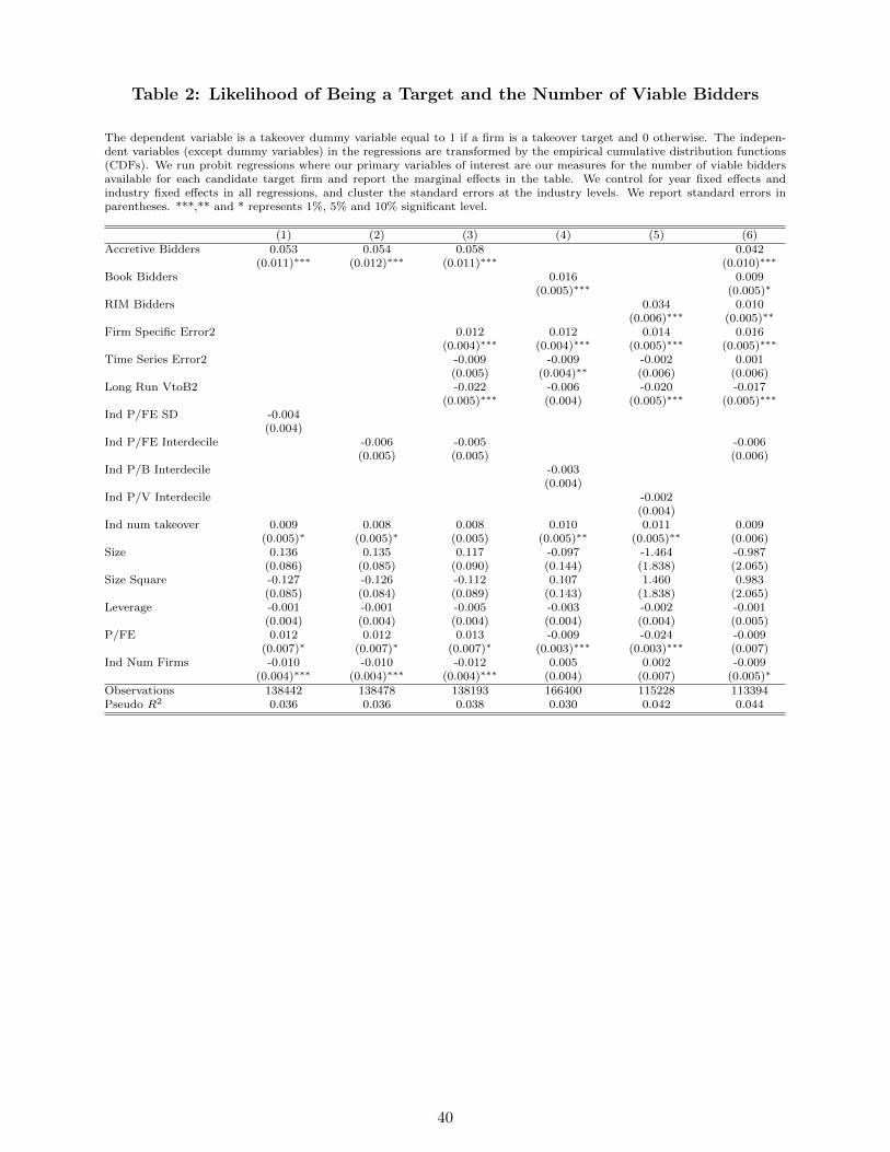
Table 2: Likelihood of Being a Target and the Number of Viable Bidders
The dependent variable is a takeover dummy variable equal to 1 if a firm is a takeover target and 0 otherwise. The indepen-dent variables (except dummy variables) in the regressions are transformed by the empirical cumulative distribution functions(CDFs). We run probit regressions where our primary variables of interest are our measures for the number of viable biddersavailable for each candidate target firm and report the marginal effects in the table. We control for year fixed effects andindustry fixed effects in all regressions, and cluster the standard errors at the industry levels. We report standard errors inparentheses. ***,** and * represents 1%, 5% and 10% significant level.
(1) (2) (3) (4) (5) (6)Accretive Bidders 0.053 0.054 0.058 0.042
(0.011)∗∗∗ (0.012)∗∗∗ (0.011)∗∗∗ (0.010)∗∗∗
Book Bidders 0.016 0.009(0.005)∗∗∗ (0.005)∗
RIM Bidders 0.034 0.010(0.006)∗∗∗ (0.005)∗∗
Firm Specific Error2 0.012 0.012 0.014 0.016(0.004)∗∗∗ (0.004)∗∗∗ (0.005)∗∗∗ (0.005)∗∗∗
Time Series Error2 -0.009 -0.009 -0.002 0.001(0.005) (0.004)∗∗ (0.006) (0.006)
Long Run VtoB2 -0.022 -0.006 -0.020 -0.017(0.005)∗∗∗ (0.004) (0.005)∗∗∗ (0.005)∗∗∗
Ind P/FE SD -0.004(0.004)
Ind P/FE Interdecile -0.006 -0.005 -0.006(0.005) (0.005) (0.006)
Ind P/B Interdecile -0.003(0.004)
Ind P/V Interdecile -0.002(0.004)
Ind num takeover 0.009 0.008 0.008 0.010 0.011 0.009(0.005)∗ (0.005)∗ (0.005) (0.005)∗∗ (0.005)∗∗ (0.006)
Size 0.136 0.135 0.117 -0.097 -1.464 -0.987(0.086) (0.085) (0.090) (0.144) (1.838) (2.065)
Size Square -0.127 -0.126 -0.112 0.107 1.460 0.983(0.085) (0.084) (0.089) (0.143) (1.838) (2.065)
Leverage -0.001 -0.001 -0.005 -0.003 -0.002 -0.001(0.004) (0.004) (0.004) (0.004) (0.004) (0.005)
P/FE 0.012 0.012 0.013 -0.009 -0.024 -0.009(0.007)∗ (0.007)∗ (0.007)∗ (0.003)∗∗∗ (0.003)∗∗∗ (0.007)
Ind Num Firms -0.010 -0.010 -0.012 0.005 0.002 -0.009(0.004)∗∗∗ (0.004)∗∗∗ (0.004)∗∗∗ (0.004) (0.007) (0.005)∗
Observations 138442 138478 138193 166400 115228 113394Pseudo R2 0.036 0.036 0.038 0.030 0.042 0.044
40
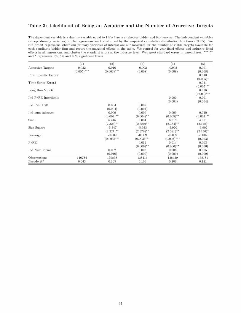
Table 3: Likelihood of Being an Acquirer and the Number of Accretive Targets
The dependent variable is a dummy variable equal to 1 if a firm is a takeover bidder and 0 otherwise. The independent variables(except dummy variables) in the regressions are transformed by the empirical cumulative distribution functions (CDFs). Werun probit regressions where our primary variables of interest are our measures for the number of viable targets available foreach candidate bidder firm and report the marginal effects in the table. We control for year fixed effects and industry fixedeffects in all regressions, and cluster the standard errors at the industry level. We report standard errors in parentheses. ***,**and * represents 1%, 5% and 10% significant levels.
(1) (2) (3) (4) (5)Accretive Targets 0.032 0.010 -0.002 -0.003 0.001
(0.005)∗∗∗ (0.003)∗∗∗ (0.008) (0.008) (0.008)Firm Specific Error2 0.010
(0.005)∗
Time Series Error2 0.011(0.005)∗∗
Long Run VtoB2 0.026(0.003)∗∗∗
Ind P/FE Interdecile 0.000 0.001(0.004) (0.004)
Ind P/FE SD 0.004 0.002(0.004) (0.004)
Ind num takeover 0.009 0.009 0.009 0.010(0.004)∗∗ (0.004)∗∗ (0.005)∗∗ (0.004)∗∗
Size 5.445 6.031 6.018 4.001(2.323)∗∗ (2.380)∗∗ (2.384)∗∗ (2.148)∗
Size Square -5.347 -5.933 -5.920 -3.902(2.321)∗∗ (2.378)∗∗ (2.381)∗∗ (2.146)∗
Leverage -0.009 -0.009 -0.009 -0.002(0.003)∗∗∗ (0.003)∗∗∗ (0.003)∗∗∗ (0.003)
P/FE 0.014 0.014 0.003(0.006)∗∗ (0.006)∗∗ (0.006)
Ind Num Firms 0.002 0.006 0.006 0.005(0.010) (0.009) (0.009) (0.009)
Observations 140784 139838 138416 138439 138181Pseudo R2 0.043 0.105 0.106 0.106 0.111
41
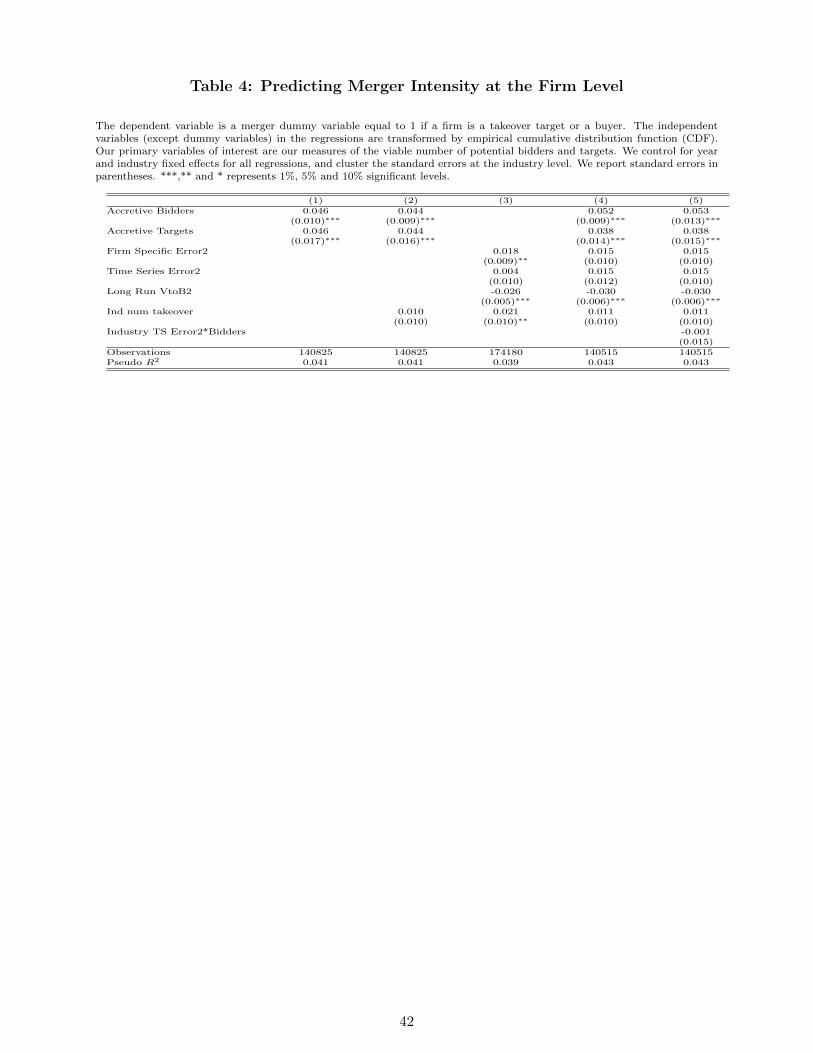
Table 4: Predicting Merger Intensity at the Firm Level
The dependent variable is a merger dummy variable equal to 1 if a firm is a takeover target or a buyer. The independentvariables (except dummy variables) in the regressions are transformed by empirical cumulative distribution function (CDF).Our primary variables of interest are our measures of the viable number of potential bidders and targets. We control for yearand industry fixed effects for all regressions, and cluster the standard errors at the industry level. We report standard errors inparentheses. ***,** and * represents 1%, 5% and 10% significant levels.
(1) (2) (3) (4) (5)Accretive Bidders 0.046 0.044 0.052 0.053
(0.010)∗∗∗ (0.009)∗∗∗ (0.009)∗∗∗ (0.013)∗∗∗
Accretive Targets 0.046 0.044 0.038 0.038(0.017)∗∗∗ (0.016)∗∗∗ (0.014)∗∗∗ (0.015)∗∗∗
Firm Specific Error2 0.018 0.015 0.015(0.009)∗∗ (0.010) (0.010)
Time Series Error2 0.004 0.015 0.015(0.010) (0.012) (0.010)
Long Run VtoB2 -0.026 -0.030 -0.030(0.005)∗∗∗ (0.006)∗∗∗ (0.006)∗∗∗
Ind num takeover 0.010 0.021 0.011 0.011(0.010) (0.010)∗∗ (0.010) (0.010)
Industry TS Error2*Bidders -0.001(0.015)
Observations 140825 140825 174180 140515 140515Pseudo R2 0.041 0.041 0.039 0.043 0.043
42

Table
5:PredictingM
erg
erIn
tensity
atth
eIn
dustry
Level
Th
ed
epen
den
tvari
ab
leis
the
cou
nt
of
mer
ger
an
nou
nce
men
tsin
ind
ust
ryj,
yea
rt.
Th
ein
dep
end
ent
vari
ab
les
incl
ud
eth
eaver
age
nu
mb
erof
bid
der
sin
ind
ust
ryj,
the
tota
lnu
mb
erof
firm
sin
ind
ust
ryj,
the
log
valu
eof
ind
ust
ryaver
age
mark
etto
book
rati
o,
the
ind
ust
ryaver
age
tim
ese
ries
erro
r,th
ein
du
stry
aver
age
of
lon
gru
nvalu
eto
book
rati
o.
All
valu
esare
lagged
.W
eals
oin
clu
de
the
tota
lnu
mb
erof
mer
ger
sat
yea
rt-
1an
dth
eto
tal
nu
mb
erof
mer
ger
sin
ind
ust
ryj.
We
contr
ol
for
yea
rfi
xed
effec
tsin
all
regre
ssio
ns
exce
pt
inco
lum
n4,
6,
8an
d10,
inw
hic
hw
eu
seT
ota
lM
erger
sat
Yea
rt.
We
contr
ol
for
ind
ust
ryfi
xed
effec
tsex
cep
tin
colu
mn
5,
6,
9an
d10,
inw
hic
hw
ein
stea
du
seth
eT
ota
lM
erger
sin
Ind
ust
ryj.
We
rep
ort
stan
dard
erro
rsin
pare
nth
eses
.***,*
*an
d*
rep
rese
nts
1%
,5%
an
d10%
sign
ifica
nt
level
s.
(1)
(2)
(3)
(4)
(5)
(6)
(7)
(8)
(9)
(10)
Ind
Aver
age
Acc
reti
ve
Bid
der
s0.1
93∗∗
∗0.1
57∗∗
∗0.1
56∗∗
∗0.1
60∗∗
∗0.0
548∗∗
∗0.0
564∗∗
∗0.1
56∗∗
∗0.1
60∗∗
∗0.0
552∗∗
∗0.0
567∗∗
∗
(39.8
6)
(18.5
2)
(18.1
9)
(18.8
2)
(8.1
7)
(8.4
2)
(18.1
7)
(18.7
9)
(8.2
1)
(8.4
5)
Ind
Nu
mF
irm
s0.0
114∗∗
∗0.0
114∗∗
∗0.0
103∗∗
∗0.0
0153
0.0
0117
0.0
114∗∗
∗0.0
103∗∗
∗0.0
0150
0.0
0115
(5.0
7)
(5.0
0)
(4.5
3)
(0.9
4)
(0.7
2)
(5.0
0)
(4.5
5)
(0.9
3)
(0.7
1)
Ind
Aver
age
M/B
1.5
64∗∗
∗1.5
25∗∗
∗-1
.492∗∗
∗-0
.899∗∗
(3.0
4)
(3.5
9)
(-3.4
7)
(-2.2
9)
Ind
Aver
age
Tim
eS
erie
sE
rror
1.5
66∗∗
∗1.5
15∗∗
∗-1
.398∗∗
∗-0
.817∗∗
(3.0
3)
(3.5
4)
(-3.1
6)
(-2.0
2)
Ind
Aver
age
lon
g-r
un
Vto
B1.5
85∗∗
∗1.5
67∗∗
∗-1
.556∗∗
∗-0
.960∗∗
(3.0
1)
(3.5
8)
(-3.5
9)
(-2.4
1)
Tota
lM
erger
sY
ear
t-1
0.0
0163∗∗
∗0.0
0493∗∗
∗0.0
0163∗∗
∗0.0
0490∗∗
∗
(4.4
5)
(11.1
4)
(4.4
6)
(11.0
1)
Tota
lM
erger
sIn
dj
0.0
121∗∗
∗0.0
120∗∗
∗0.0
121∗∗
∗0.0
120∗∗
∗
(26.5
9)
(26.4
3)
(26.5
4)
(26.3
8)
Ob
serv
ati
on
s2136
1981
1923
1923
1923
1923
1922
1922
1922
1922
R2
0.8
70
0.8
66
0.8
66
0.8
62
0.7
77
0.7
71
0.8
66
0.8
62
0.7
78
0.7
71
43

Table
6a:PredictingM
eth
od
ofPaymentatth
eFirm
Level
Th
ed
epen
den
tvari
ab
leis
ad
um
my
vari
ab
leeq
ual
to1
ifth
ed
eal
on
lyu
ses
stock
as
met
hod
of
paym
ent
an
d0
oth
erw
ise.
Th
ein
dep
end
ent
vari
ab
les
(exce
pt
du
mm
yvari
ab
les)
inth
ere
gre
ssio
ns
are
tran
sform
edby
the
emp
iric
al
cum
ula
tive
dis
trib
uti
on
fun
ctio
n(C
DF
).T
he
contr
ol
vari
ab
les
incl
ud
eth
est
an
dard
dev
iati
on
of
the
targ
et’s
ind
ust
ryP
/F
E(i
nco
lum
n1),
the
targ
et’s
ind
ust
ryP
/F
Ein
terd
ecile
ran
ge
(colu
mn
2,
3,
an
d4),
the
targ
et’s
ind
ust
ryP
/B
inte
rdec
ile
ran
ge
(colu
mn
5),
targ
et’s
ind
ust
ryP
/V
inte
rdec
ile
ran
ge
(colu
mn
6).
Inad
dit
ion
,in
all
colu
mn
sw
eco
ntr
ol
for
the
nu
mb
erof
dea
lsin
targ
et’s
ind
ust
ry,
the
targ
et’s
size
an
dsi
zesq
uare
d,
the
targ
et’s
lever
age,
the
targ
et’s
P/F
E,
the
nu
mb
erof
firm
sin
targ
et’s
ind
ust
ryan
da
du
mm
yvari
ab
lew
hic
heq
uals
to1
ifth
ed
eal
iste
nd
eroff
eran
d0
oth
erw
ise.
Fro
mco
lum
n4,
we
als
oin
clu
de
the
acq
uir
er’s
info
rmati
on
incl
ud
ing
acq
uir
er’s
size
,le
ver
age,
P/F
E,
acq
uir
er’s
ind
ust
ryP
/F
Ein
terd
ecile,
acq
uir
er’s
ind
ust
ryP
/B
inte
rdec
ile,
an
dacq
uir
er’s
ind
ust
ryP
/V
inte
rdec
ile.
To
save
space
,w
ed
on
ot
rep
ort
the
coeffi
cien
tsof
thes
eco
ntr
ol
vari
ab
les.
We
run
pro
bit
regre
ssio
ns
an
dre
port
the
marg
inal
effec
tsin
the
tab
le.
We
contr
ol
for
yea
rfi
xed
effec
tsan
din
du
stry
fixed
effec
tsin
all
regre
ssio
ns
an
dcl
ust
erth
est
an
dard
erro
rsat
the
ind
ust
ryle
vel
.W
ere
port
stan
dard
erro
rsin
pare
nth
eses
.***,*
*an
d*
rep
rese
nts
1%
,5%
an
d10%
sign
ifica
nt
level
s.
(1)
(2)
(3)
(4)
(5)
(6)
Targ
et
Accre
tive
Bid
ders
0.1
74
0.1
60
0.1
09
0.2
51
(0.1
02)∗
(0.1
03)
(0.1
07)
(0.0
99)∗
∗∗
Targ
et
Accre
tive
Targ
ets
0.1
08
0.1
24
0.1
55
0.1
98
(0.0
85)
(0.0
82)
(0.0
75)∗
∗(0
.060)∗
∗∗
Targ
et
Book
Bid
ders
0.0
39
(0.0
72)
Targ
et
Book
Targ
ets
0.1
76
(0.0
42)∗
∗∗
Targ
et
RIM
Bid
ders
0.1
16
(0.0
77)
Targ
et
RIM
Targ
ets
0.0
67
(0.0
53)
Acqu
irer
Accre
tive
Bid
ders
0.0
04
(0.0
56)
Acqu
irer
Accre
tive
Targ
ets
-0.0
01
(0.0
56)
Acqu
irer
Book
Bid
ders
-0.1
23
(0.0
52)∗
∗
Acqu
irer
Book
Targ
ets
0.1
54
(0.0
56)∗
∗∗
Acqu
irer
RIM
Bid
ders
0.0
68
(0.0
53)
Acqu
irer
RIM
Targ
ets
0.0
32
(0.0
61)
Targ
et
Fir
mS
pecifi
cE
rror2
0.0
02
-0.0
16
-0.1
00
-0.0
26
(0.0
60)
(0.0
93)
(0.0
64)
(0.1
05)
Targ
et
Tim
eS
eri
es
Err
or2
0.1
72
0.2
07
0.2
21
0.1
78
(0.0
61)∗
∗∗
(0.1
04)∗
∗(0
.082)∗
∗∗
(0.1
10)
Targ
et
Lon
gR
un
Vto
B2
0.1
14
0.1
54
0.0
82
0.1
74
(0.0
50)∗
∗(0
.063)∗
∗(0
.058)
(0.0
54)∗
∗∗
Acqu
irer
Fir
mS
pecifi
cE
rror2
0.2
04
0.1
69
0.1
62
(0.0
59)∗
∗∗
(0.0
57)∗
∗∗
(0.0
56)∗
∗∗
Acqu
irer
Tim
eS
eri
es
Err
or2
-0.0
27
-0.1
43
0.0
30
(0.0
70)
(0.0
71)∗
∗(0
.061)
Acqu
irer
Lon
gR
un
Vto
B2
0.0
69
-0.0
93
0.0
88
(0.0
45)
(0.0
46)∗
∗(0
.058)
Ob
serv
ati
on
s5339
5339
5336
3295
4353
2735
Pse
ud
oR
20.2
08
0.2
10
0.2
18
0.2
35
0.2
32
0.2
54
44

Table
6b:PredictingM
eth
od
ofPaymentatth
eIn
dustry
Level
Th
ed
epen
den
tvari
ab
leis
the
cou
nt
of
100%
stock
-fin
an
ced
mer
ger
an
nou
nce
men
tsin
ind
ust
ryj,
yea
rt.
Th
ein
dep
end
ent
vari
ab
les
incl
ud
eth
eaver
age
nu
mb
erof
bid
der
sin
ind
ust
ryj,
the
tota
lnu
mb
erof
firm
sin
ind
ust
ryj,
the
log
valu
eof
ind
ust
ryaver
age
mark
etto
book
rati
o,
the
ind
ust
ryaver
age
tim
ese
ries
erro
r,th
ein
du
stry
aver
age
of
lon
gru
nvalu
eto
book
rati
o.
All
valu
esare
lagged
.W
eals
oin
clu
de
the
tota
lnu
mb
erof
mer
ger
sat
yea
rt-
1an
dth
eto
tal
nu
mb
erof
mer
ger
sin
ind
ust
ryj.
We
contr
ol
for
yea
rfi
xed
effec
tsin
all
regre
ssio
ns
exce
pt
inco
lum
n4,
6,
8an
d10,
inw
hic
hw
eu
seT
ota
lM
erger
sat
Yea
rt.
We
contr
ol
for
ind
ust
ryfi
xed
effec
tsex
cep
tin
colu
mn
5,
6,
9an
d10,
inw
hic
hw
ein
stea
du
seth
eT
ota
lM
erger
sin
Ind
ust
ryj.
We
rep
ort
stan
dard
erro
rsin
pare
nth
eses
.***,*
*an
d*
rep
rese
nts
1%
,5%
an
d10%
sign
ifica
nt
level
s.
(1)
(2)
(3)
(4)
(5)
(6)
(7)
(8)
(9)
(10)
Ind
Aver
age
Acc
reti
ve
Bid
der
s0.2
35∗∗
∗0.2
38∗∗
∗0.2
37∗∗
∗0.2
41∗∗
∗0.0
687∗∗
∗0.0
711∗∗
∗0.2
37∗∗
∗0.2
41∗∗
∗0.0
692∗∗
∗0.0
716∗∗
∗
(33.4
3)
(19.2
1)
(18.8
9)
(19.3
5)
(7.3
4)
(7.6
1)
(18.8
8)
(19.3
3)
(7.3
9)
(7.6
5)
Ind
Nu
mF
irm
s-0
.00211
-0.0
0217
-0.0
0287
-0.0
0302
-0.0
0334
-0.0
0218
-0.0
0287
-0.0
0306
-0.0
0338
(-0.6
5)
(-0.6
5)
(-0.8
7)
(-1.3
4)
(-1.4
8)
(-0.6
6)
(-0.8
7)
(-1.3
5)
(-1.4
9)
Ind
Aver
age
M/B
1.9
08∗∗
1.3
86∗∗
-1.7
61∗∗
∗-1
.318∗∗
(2.5
4)
(2.2
4)
(-2.9
4)
(-2.4
1)
Ind
Aver
age
Tim
eS
erie
sE
rror
1.9
30∗∗
1.3
94∗∗
-1.6
14∗∗
∗-1
.192∗∗
(2.5
6)
(2.2
4)
(-2.6
1)
(-2.1
2)
Ind
Aver
age
lon
g-r
un
Vto
B1.8
92∗∗
1.3
96∗∗
-1.8
45∗∗
∗-1
.399∗∗
(2.4
6)
(2.1
9)
(-3.0
5)
(-2.5
2)
Tota
lM
erger
sY
ear
t-1
0.0
0125∗∗
0.0
0548∗∗
∗0.0
0124∗∗
0.0
0543∗∗
∗
(2.3
4)
(8.8
8)
(2.3
3)
(8.7
5)
Tota
lM
erger
sIn
dj
0.0
0799∗∗
∗0.0
0783∗∗
∗0.0
0797∗∗
∗0.0
0781∗∗
∗
(12.6
0)
(12.3
5)
(12.5
6)
(12.3
1)
Ob
serv
ati
on
s2136
1981
1923
1923
1923
1923
1922
1922
1922
1922
R2
0.7
04
0.6
88
0.6
89
0.6
81
0.5
29
0.5
17
0.6
89
0.6
81
0.5
30
0.5
17
45

Table
7:Likelihood
ofHorizo
ntalM
erg
ers
and
theNumberofViable
Bidders
and
Targ
ets
Th
ed
epen
den
tvari
ab
leis
hori
zonta
ld
um
my
vari
ab
leeq
ual
to1
ifth
ed
eal
hap
pen
edb
etw
een
two
firm
sw
ith
inth
esa
me
two
dig
itS
ICin
du
stry
an
d0
oth
erw
ise.
Th
ein
dep
end
ent
vari
ab
les
(exce
pt
du
mm
yvari
ab
les)
inth
ere
gre
ssio
ns
are
tran
sform
edby
emp
iric
al
cum
ula
tive
dis
trib
uti
on
fun
ctio
n(C
DF
).W
eru
np
rob
itre
gre
ssio
ns
wh
ere
ou
rp
rim
ary
mea
sure
sare
the
nu
mb
erof
via
ble
bid
der
san
dta
rget
savailab
leto
each
firm
,an
dre
port
the
marg
inal
effec
tsin
the
tab
le.
We
contr
ol
for
yea
rfi
xed
effec
tin
all
regre
ssio
ns
an
din
du
stry
fixed
effec
tsfr
om
colu
mn
s4
to6,
an
dcl
ust
erth
est
an
dard
erro
rsat
the
ind
ust
ryle
vel
.W
ere
port
stan
dard
erro
rsin
pare
nth
eses
.***,*
*an
d*
rep
rese
nts
1%
,5%
an
d10%
sign
ifica
nt
level
s.
(1)
(2)
(3)
(4)
(5)
(6)
Targ
etA
ccre
tive
Bid
der
s0.2
64
0.0
28
(0.1
07)∗
∗(0
.048)
Targ
etA
ccre
tive
Targ
ets
0.1
68
0.0
24
(0.0
52)∗
∗∗(0
.072)
Targ
etB
ook
Bid
der
s0.2
37
0.1
15
(0.0
76)∗
∗∗(0
.072)
Targ
etB
ook
Targ
ets
0.1
68
0.0
48
(0.0
68)∗
∗(0
.065)
Targ
etR
IMB
idd
ers
0.2
72
0.0
82
(0.0
97)∗
∗∗(0
.055)
Targ
etR
IMT
arg
ets
0.2
07
0.0
44
(0.0
57)∗
∗∗(0
.067)
Ob
serv
ati
on
s5431
6346
4695
5398
6306
4666
Pse
ud
oR
20.0
59
0.0
53
0.0
67
0.1
64
0.1
57
0.1
70
46
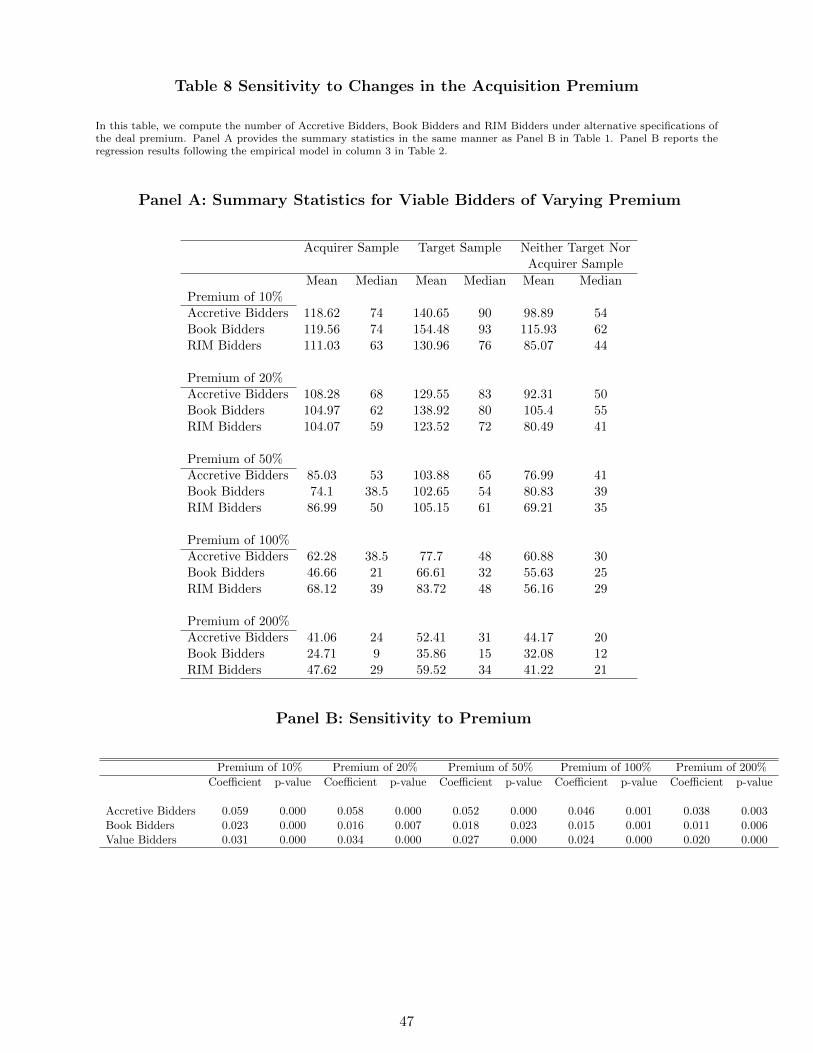
Table 8 Sensitivity to Changes in the Acquisition Premium
In this table, we compute the number of Accretive Bidders, Book Bidders and RIM Bidders under alternative specifications ofthe deal premium. Panel A provides the summary statistics in the same manner as Panel B in Table 1. Panel B reports theregression results following the empirical model in column 3 in Table 2.
Panel A: Summary Statistics for Viable Bidders of Varying Premium
Acquirer Sample Target Sample Neither Target NorAcquirer Sample
Mean Median Mean Median Mean MedianPremium of 10%Accretive Bidders 118.62 74 140.65 90 98.89 54Book Bidders 119.56 74 154.48 93 115.93 62RIM Bidders 111.03 63 130.96 76 85.07 44
Premium of 20%Accretive Bidders 108.28 68 129.55 83 92.31 50Book Bidders 104.97 62 138.92 80 105.4 55RIM Bidders 104.07 59 123.52 72 80.49 41
Premium of 50%Accretive Bidders 85.03 53 103.88 65 76.99 41Book Bidders 74.1 38.5 102.65 54 80.83 39RIM Bidders 86.99 50 105.15 61 69.21 35
Premium of 100%Accretive Bidders 62.28 38.5 77.7 48 60.88 30Book Bidders 46.66 21 66.61 32 55.63 25RIM Bidders 68.12 39 83.72 48 56.16 29
Premium of 200%Accretive Bidders 41.06 24 52.41 31 44.17 20Book Bidders 24.71 9 35.86 15 32.08 12RIM Bidders 47.62 29 59.52 34 41.22 21
Panel B: Sensitivity to Premium
Premium of 10% Premium of 20% Premium of 50% Premium of 100% Premium of 200%
Coefficient p-value Coefficient p-value Coefficient p-value Coefficient p-value Coefficient p-value
Accretive Bidders 0.059 0.000 0.058 0.000 0.052 0.000 0.046 0.001 0.038 0.003Book Bidders 0.023 0.000 0.016 0.007 0.018 0.023 0.015 0.001 0.011 0.006Value Bidders 0.031 0.000 0.034 0.000 0.027 0.000 0.024 0.000 0.020 0.000
47
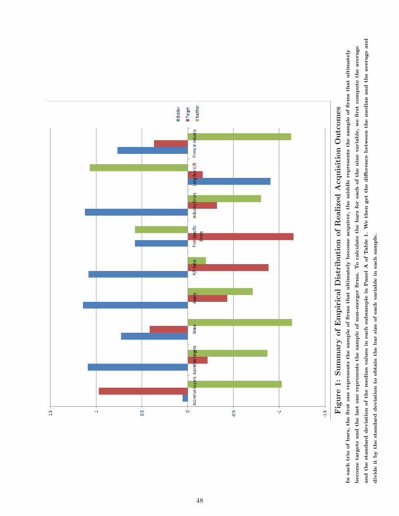
Figure
1:Summary
ofEmpiricalDistribution
ofRealize
dAcq
uisition
Outcomes
Ineach
trio
of
bars,
the
first
on
erep
rese
nts
the
sam
ple
of
firm
sth
at
ult
imate
lyb
ecom
eacqu
irer,
the
mid
dle
rep
rese
nts
the
sam
ple
of
firm
sth
at
ult
imate
ly
becom
eta
rgets
an
dth
ela
ston
erep
rese
nts
the
sam
ple
of
non
-merger
firm
s.T
ocalc
ula
teth
eb
ars
for
each
of
the
nin
evaria
ble
,w
efi
rst
com
pu
teth
eaverage
an
dth
est
an
dard
devia
tion
of
the
med
ian
valu
es
ineach
sub
sam
ple
inP
an
el
Aof
Tab
le1.
We
then
get
the
diff
eren
ce
betw
een
the
med
ian
an
dth
eaverage
an
d
div
ide
itby
the
stan
dard
devia
tion
toob
tain
the
bar
size
of
each
varia
ble
ineach
sam
ple
.
48

Cal
year
1981
1982
1983
1984
1985
1986
1987
1988
1989
1990
1991
1992
1993
1994
1995
1996
1997
1998
1999
2000
2001
2002
2003
2004
2005
2006
2007
2008
2009
2010
2011
2012
Tot
alN
um
ber
Dea
ls93
8894
135
151
191
197
229
202
133
125
110
189
287
346
356
448
494
472
403
296
164
177
185
167
200
216
177
137
148
103
119
Med
ian
Acc
reti
veB
idd
ers
3436
3638
4141
42.5
4545
4545
4647
5962
6468
6868
6563
6158
5656
5653
4949
4442
43S
&P
Ind
ex12
314
116
516
721
124
224
727
835
333
041
743
646
645
961
674
197
012
2914
6913
2011
4888
011
1212
1212
4814
1814
6890
311
1512
5812
5814
26M
/BD
isp
ersi
on4.
083.
414.
883.
874.
344.
924.
834.
194.
944.
355.
645.
355.
374.
395.
385.
655.
575.
928.
556.
495.
173.
964.
995.
144.
925.
185.
663.
704.
334.
714.
574.
89
Figure
2:KeyVariablesAcross
Tim
eT
he
sam
ple
isth
esa
mp
lein
the
regress
ion
of
colu
mn
3in
Tab
le2,
coverin
gp
erio
dfr
om
1981
to2012.
Th
enu
mb
er
of
deals
of
pu
bli
cfi
rm
s(t
ota
lnu
mb
er)
is
the
tota
lnu
mb
er
of
deals
an
nou
nced
.T
he
level
of
S&
P500
(sp
ind
x)
isth
enu
mb
er
at
the
en
dof
cale
nd
ar
year.
We
calc
ula
teth
em
ed
ian
level
of
dis
persi
on
(inte
rd
ecil
e)
of
Market
toB
ook
rati
o(m
tbd
isp
ersi
on
)an
dth
em
ed
ian
of
lag
valu
es
of
the
num
ber
of
Accreti
ve
Bid
ders
(med
ian
accreti
ve
bid
ders)
each
year.
We
scale
each
plo
taccord
ing
toth
eactu
al
ran
ge
of
corresp
on
din
gse
rie
s.T
he
data
tab
leis
provid
ed
belo
wth
egrap
h.
49

Figure 3: Actual Takeovers among Depository InstitutionsThe sample is the sample in the regression of column 3 in Table 2, covering period from 1981 to 2012. The
total ind takeover is the total number of deals announced in the depository industry (SIC code 60) in each
year. We calculate the total number of firms (total num firms), the median of lag values of the number of
Accretive Bidders (median feps bidders), Book Bidders (median book bidders) and RIM based value Bidders
(median value bidders) for each year.
50

Figure 4: Actual Takeovers among Business Services FirmsThe sample is the sample in the regression of column 3 in Table 2, covering period from 1981 to 2012. The
total ind takeover is the total number of deals announced in the business service industry (SIC code 73) in
each year. We calculate the total number of firms (total num firms), the median of lag values of the number
of Accretive Bidders (median feps bidders), Book Bidders (median book bidders) and RIM based value
Bidders (median value bidders) for each year.
51
Top Related