


Languages
Pages
Legal


Vol. 6, No. 3, 2010 ISSN 1556-6706
SCIENTIA MAGNA
An international journal
Edited by
Department of Mathematics Northwest University
Xi’an, Shaanxi, P.R.China

i
Scientia Magna is published annually in 400-500 pages per volume and 1,000 copies. It is also available in microfilm format and can be ordered (online too) from:
Books on Demand ProQuest Information & Learning 300 North Zeeb Road P.O. Box 1346 Ann Arbor, Michigan 48106-1346, USA Tel.: 1-800-521-0600 (Customer Service) URL: http://wwwlib.umi.com/bod/ Scientia Magna is a referred journal: reviewed, indexed, cited by the following journals: "Zentralblatt Für Mathematik" (Germany), "Referativnyi Zhurnal" and "Matematika" (Academia Nauk, Russia), "Mathematical Reviews" (USA), "Computing Review" (USA), Institute for Scientific Information (PA, USA), "Library of Congress Subject Headings" (USA).
Printed in the United States of America Price: US$ 69.95

ii
Information for Authors
Papers in electronic form are accepted. They can be e-mailed in Microsoft Word XP (or lower), WordPerfect 7.0 (or lower), LaTeX and PDF 6.0 or lower.
The submitted manuscripts may be in the format of remarks, conjectures, solved/unsolved or open new proposed problems, notes, articles, miscellaneous, etc. They must be original work and camera ready [typewritten/computerized, format: 8.5 x 11 inches (21,6 x 28 cm)]. They are not returned, hence we advise the authors to keep a copy.
The title of the paper should be writing with capital letters. The author's name has to apply in the middle of the line, near the title. References should be mentioned in the text by a number in square brackets and should be listed alphabetically. Current address followed by e-mail address should apply at the end of the paper, after the references.
The paper should have at the beginning an abstract, followed by the keywords. All manuscripts are subject to anonymous review by three independent
reviewers. Every letter will be answered. Each author will receive a free copy of the journal.

iii
Contributing to Scientia Magna Authors of papers in science (mathematics, physics, philosophy, psychology,
sociology, linguistics) should submit manuscripts, by email, to the Editor-in-Chief:
Prof. Wenpeng Zhang Department of Mathematics Northwest University Xi’an, Shaanxi, P.R.China E-mail: [email protected]
Or anyone of the members of Editorial Board: Dr. W. B. Vasantha Kandasamy, Department of Mathematics, Indian Institute of Technology, IIT Madras, Chennai - 600 036, Tamil Nadu, India. Dr. Larissa Borissova and Dmitri Rabounski, Sirenevi boulevard 69-1-65, Moscow 105484, Russia. Dr. Zhaoxia Wu, School of Applied Mathematics, Xinjiang University of Finance and Economics, Urmq, P.R.China. E-mail: [email protected] Prof. Yuan Yi, Research Center for Basic Science, Xi’an Jiaotong University, Xi’an, Shaanxi, P.R.China. E-mail: [email protected] Dr. Zhefeng Xu, Department of Mathematic s, Northwest University, Xi’an, Shaanxi, P.R.China. E-mail: [email protected]; [email protected] Prof. József Sándor, Babes-Bolyai University of Cluj, Romania. E-mail: [email protected]; [email protected] Dr. Xia Yuan, Department of Mathematics, Northwest University, Xi’an, Shaanxi, P.R.China. E-mail: [email protected]

Contents
R. Vasuki and A. Nagarajan : Further results on mean graphs 1
S. Gao and Q. Zheng : A short interval result for the exponential
divisor function 15
C. Shi : On the mean value of some new sequences 20
Q. Zheng and S. Gao : A short interval result for the exponential
Mobius function 25
W. Liu and Z. Chang : Approach of wavelet estimation in a
semi-parametric regression model with ρ-mixing errors 29
A. Nawzad, etc. : Generalize derivations on semiprime rings 34
A. Nagarajan, etc. : Near meanness on product graphs 40
H. Liu : Super-self-conformal sets 50
M. K. Karacan and Y. Tuncer : Tubular W-surfaces
in 3-space 55
E. Turhan and T. Korpinar : Integral Formula in Special
Three-Dimansional Kenmotsu Manifold K with η− Parallel Ricci Tensor 63
L. Dai, etc. : Iterative method for the solution of linear matrix
equation AXBT + CY DT = F 71
P. S. K. Reddy, etc. : Smarandachely antipodal signed digraphs 84
P. S. K. Reddy, etc. : Smarandachely t-path step signed graphs 89
W. Huang and J. Zhao : On a note of the Smarandache power function 93
R. Sridevi, etc. : Almost super Fibonacci graceful labeling 99
iv
Scientia MagnaVol. 6 (2010), No. 3, 1-14
Further results on mean graphs
R. Vasuki† and A. Nagarajan‡
† Department of Mathematics, Dr. Sivanthi Aditanar College of Engineering,Tiruchendur 628215, Tamil Nadu, India
‡ Department of Mathematics, V. O. Chidambaram College, Thoothukudi 628008,Tamil Nadu, India
E-mail: [email protected] [email protected]
Abstract Let G(V, E) be a graph with p vertices and q edges. For every assignment
f : V (G) → 0, 1, 2, 3, . . . , q, an induced edge labeling f∗ : E(G) → 1, 2, 3 . . . , q is de-
fined by
f∗(uv) =
f(u)+f(v)2
, if f(u) and f(v) are of the same parity,
f(u)+f(v)+12
, otherwise.
for every edge uv ∈ E(G). If f∗(E) = 1, 2, . . . , q, then we say that f is a mean labeling of
G. If a graph G admits a mean labeling, then G is called a mean graph. In this paper we
study the meanness of the splitting graph of the path Pn and C2n(n ≥ 2), meanness of some
duplicate graphs, meanness of Armed crown, meanness of Bi-armed crown and mean labeling
of cyclic snakes.
Keywords Mean labeling, splitting graphs, duplicate graphs, armed crown, cyclic snake.
§1. Introduction
Throughout this paper, by a graph we mean a finite, undirected, simple graph. Let G(V, E)be a graph with p vertices and q edges. For notations and terminology we follow [1].
Path on n vertices is denoted by Pn and cycle on n vertices is denoted by Cn. K1,m iscalled a star and it is denoted by Sm. The graph K2 × K2 × K2 is called the cube and it isdenoted by Q3. The Union of two graphs G1 and G2 is the graph G1UG2 with V (G1UG2) =V (G1)UV (G2) and E(G1UG2) = E(G1)UE(G2). The union of m disjoint copies of a graph G
is denoted by mG. The H−graph of a path Pn is the graph obtained from two copies of Pn
with vertices v1, v2, . . . , vn and u1, u2, . . . , un by joining the vertices vn+12
and un+12
by an edgeif n is odd and the vertices vn
2 +1 and un2
if n is even.
A vertex labeling of G is an assignment f : V (G) → 0, 1, 2, . . . , q. For a vertex labelingf , the induced edge labeling f? is defined by
f∗(uv) = f(u)+f(v)2 for any edge uv in G, that is,
2 R. Vasuki and A. Nagarajan No. 3
f∗(uv) =
f(u)+f(v)2 , if f(u) and f(v) are of same parity,
f(u)+f(v)+12 , otherwise.
A vertex labeling f is called a mean labeling of G if its induced edge labeling f∗ : E →1, 2, . . . , q is a bijection, that is, f∗(E) = 1, 2, . . . , q. If a graph G has a mean labeling,then we say that G is a mean graph.
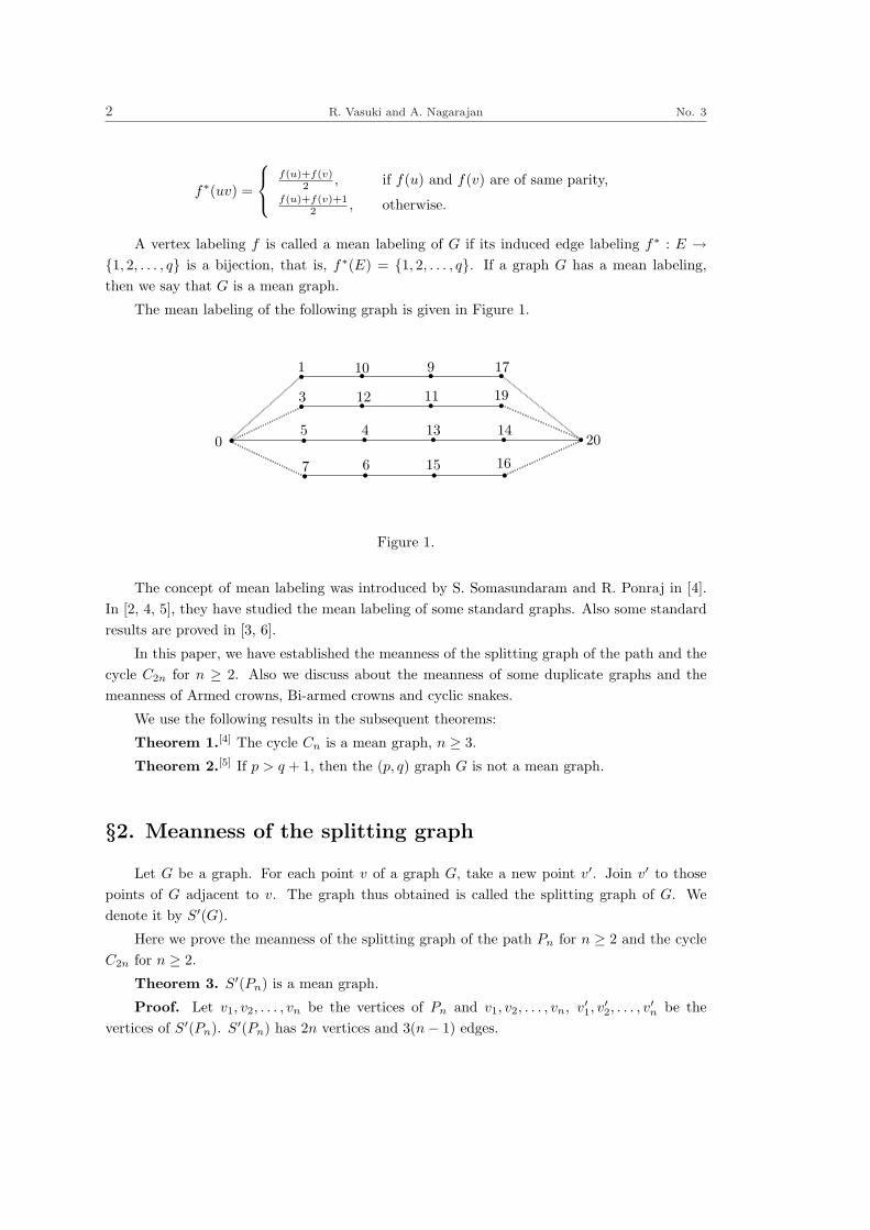
The mean labeling of the following graph is given in Figure 1.
r rr r
r rr r
r rr r
r rr r
rr0
1 10 9 17
3 12 11 19
5 4 13 14
7 6 15 16
20
Figure 1.
The concept of mean labeling was introduced by S. Somasundaram and R. Ponraj in [4].In [2, 4, 5], they have studied the mean labeling of some standard graphs. Also some standardresults are proved in [3, 6].
In this paper, we have established the meanness of the splitting graph of the path and thecycle C2n for n ≥ 2. Also we discuss about the meanness of some duplicate graphs and themeanness of Armed crowns, Bi-armed crowns and cyclic snakes.
We use the following results in the subsequent theorems:
Theorem 1.[4] The cycle Cn is a mean graph, n ≥ 3.
Theorem 2.[5] If p > q + 1, then the (p, q) graph G is not a mean graph.
§2. Meanness of the splitting graph
Let G be a graph. For each point v of a graph G, take a new point v′. Join v′ to thosepoints of G adjacent to v. The graph thus obtained is called the splitting graph of G. Wedenote it by S′(G).
Here we prove the meanness of the splitting graph of the path Pn for n ≥ 2 and the cycleC2n for n ≥ 2.
Theorem 3. S′(Pn) is a mean graph.
Proof. Let v1, v2, . . . , vn be the vertices of Pn and v1, v2, . . . , vn, v′1, v′2, . . . , v
′n be the
vertices of S′(Pn). S′(Pn) has 2n vertices and 3(n− 1) edges.

Vol. 6 Further results on mean graphs 3
We define f : V ((S′(Pn)) → 0, 1, 2, . . . , q by
f(v2i+1) = 2i, 0 ≤ i ≤⌊
n− 12
⌋,
f(v2i) = 2n− 1 + 2(i− 1), 1 ≤ i ≤⌊n
2
⌋,
f(v′2i+1) = 2n− 2 + 2i, 0 ≤ i ≤⌊
n− 12
⌋,
f(v′2i) = 2i− 1, 1 ≤ i ≤⌊n
2
⌋.
It can be verified that the label of the edges of S′(Pn) are 1, 2, . . . , q and hence S′(Pn) isa mean graph.
For example, the mean labelings of S′(P11) and S′(P14) are shown in Figure 2.
s ss s s s s s s s s
s ss s s s s s s s s
0 21 2 23 4 25 6 27 8 29 10
20 1 22 3 24 5 26 7 28 9 30
S′(P11)
s ss s s s s s s s s
s ss s s s s s s s s0 27 2 29 4 31 6 33 8 35 10
26 28 3 30 5 32 7 34 9 361
s ss
s ss11 38 13
37 12 39
S′(P14)Figure 2.
Theorem 4. S′(C2n) is a mean graph.Proof. Let v1, v2, . . . , v2n be the vertices of the cycle C2n and v1, v2, . . . , v2n, v′1, v
′2, . . . , v
′2n
be the vertices of S′(C2n).Note that S′(C2n) has 4n vertices and 6n edges.Now we define f : V (S′(C2n)) → 0, 1, 2, . . . , q as follows:
f(v2i+1) =
4i, 0 ≤ i ≤ ⌊n2
⌋,
5 + 4((n− 1)− i),⌊
n2
⌋+ 1 ≤ i ≤ n− 1.
f(v2i) =
4n + 2 + 4i− 4, 1 ≤ i ≤ ⌈n2
⌉,
4n + 3 + 4(n− i),⌈
n2
⌉+ 1 ≤ i ≤ n.
f(v′2i+1) =
4n + 4i, 0 ≤ i ≤ ⌊n2
⌋,
4n + 5 + 4((n− 1)− i),⌊
n2
⌋+ 1 ≤ i ≤ n− 1.

4 R. Vasuki and A. Nagarajan No. 3
f(v′2i) =
2 + 4i− 4, 1 ≤ i ≤ ⌈n2
⌉,
3 + 4(n− i),⌈
n2
⌉+ 1 ≤ i ≤ n.
It can be verified that the labels of the edges of S′(C2n) are 1, 2, 3, . . . , q.
Hence S′(C2n) is a mean graph.
For example, the mean labeling of S′(C14) is shown in Figure 3.
t
t
t
t
t
t
tt
t
t
t
t
tt
t
t
t
t
t
t
tt
t
t
t
t
t
t28
2
32
6
36
10
4014
41
11
37
7
33
3
0
30
4
34
8
38
1242
13
39
9
35
531
S′(C14)
Figure 3.
The mean labelings of the splitting graph of K1,1, K1,2 and K1,3 are shown in the followingFigure 4.
aaaaaaaa
s s
s s s
ss
s
ss s
sss s
ss
s
0
2 1
3 6 2
1
05
4 0
1
3 57 8
92
S′(K1,1) S′(K1,2) S′(K1,3)
Figure 4.
Vol. 6 Further results on mean graphs 5
§3. Meanness of Duplicate Graphs
Let G be a graph with V (G) as vertex set. Let V ′ be the set of vertices with |V ′| = |V |.For each point a ∈ V , we can associate a unique point a′ ∈ V ′. The duplicate graph of G
denoted by D(G) has vertex set V ∪ V ′. If a and b are adjacent in G then a′b and ab′ areadjacent in D(G).
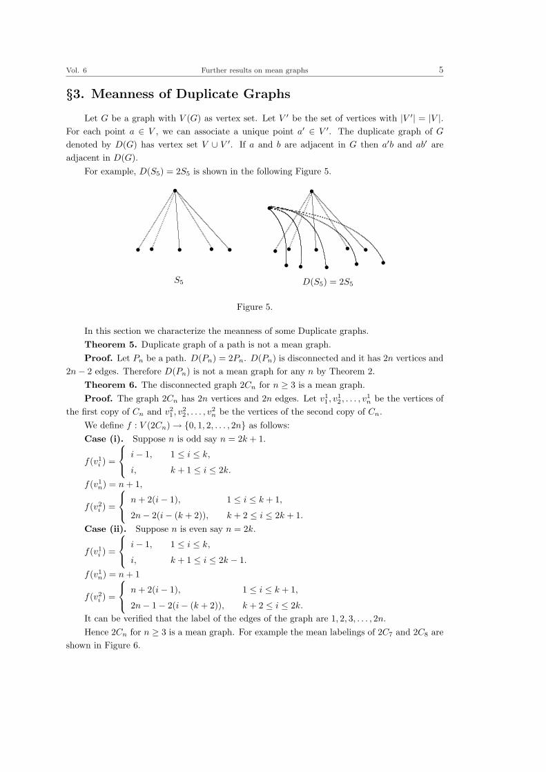
For example, D(S5) = 2S5 is shown in the following Figure 5.
s
s s s s s
S5
ss
s s s s ss s s s s
D(S5) = 2S5
Figure 5.
In this section we characterize the meanness of some Duplicate graphs.Theorem 5. Duplicate graph of a path is not a mean graph.Proof. Let Pn be a path. D(Pn) = 2Pn. D(Pn) is disconnected and it has 2n vertices and
2n− 2 edges. Therefore D(Pn) is not a mean graph for any n by Theorem 2.Theorem 6. The disconnected graph 2Cn for n ≥ 3 is a mean graph.Proof. The graph 2Cn has 2n vertices and 2n edges. Let v1
1 , v12 , . . . , v1
n be the vertices ofthe first copy of Cn and v2
1 , v22 , . . . , v2
n be the vertices of the second copy of Cn.We define f : V (2Cn) → 0, 1, 2, . . . , 2n as follows:Case (i). Suppose n is odd say n = 2k + 1.
f(v1i ) =
i− 1, 1 ≤ i ≤ k,
i, k + 1 ≤ i ≤ 2k.
f(v1n) = n + 1,
f(v2i ) =
n + 2(i− 1), 1 ≤ i ≤ k + 1,
2n− 2(i− (k + 2)), k + 2 ≤ i ≤ 2k + 1.Case (ii). Suppose n is even say n = 2k.
f(v1i ) =
i− 1, 1 ≤ i ≤ k,
i, k + 1 ≤ i ≤ 2k − 1.
f(v1n) = n + 1
f(v2i ) =
n + 2(i− 1), 1 ≤ i ≤ k + 1,
2n− 1− 2(i− (k + 2)), k + 2 ≤ i ≤ 2k.It can be verified that the label of the edges of the graph are 1, 2, 3, . . . , 2n.Hence 2Cn for n ≥ 3 is a mean graph. For example the mean labelings of 2C7 and 2C8 are
shown in Figure 6.

6 R. Vasuki and A. Nagarajan No. 3
s
sss
s s
s
0
1
2
4
5
6
8
s
sss
s s
s
7
9
11
13
14
12
10
s
ss
s
s
0
1
2
3
5
s
ss
s
s
8
10
12
14
16
s
ss
s
ss
6
7
9
15
13
11
2C7 2C8
Figure 6.
Corollary 1. Duplicate graph of the cycle Cn is a mean graph.
Proof. D(Cn) = C2n when n is odd. But C2n is a mean graph by Theorem 1 andD(Cn) = 2Cn when n is even. 2Cn is a mean graph by Theorem 6. Therefore D(Cn) is a meangraph.
Theorem 7. mQ3 is a mean graph.
Proof. For 1 ≤ j ≤ m, let vj1, v
j2, . . . , v
j8 be the vertices in the jth copy of Q3. The graph
mQ3 has 8m vertices and 12m edges. We define f : V (mQ3) → 0, 1, 2, . . . , 12m as follows.
When m = 1, label the vertices of Q3 as follows:
ss
s s
s
ss
s
0 4
12 11
8 10
2 3
For m > 1, label the vertices of mQ3 as follows:
f(vj1) = 12(j − 1), 1 ≤ j ≤ m
f(vji ) = 12(j − 1) + i, 2 ≤ i ≤ 4, 1 ≤ j ≤ m
f(vj5) = 12(j − 1) + 8, 1 ≤ j ≤ m
f(vj6) = 12(j − 1) + 9, 1 ≤ j ≤ m− 1
f(vj7) = 12(j − 1) + 11, 1 ≤ j ≤ m− 1
f(vj8) = 12j + 1, 1 ≤ j ≤ m− 1
f(vm6 ) = 12m − 2, f(vm
7 ) = 12m − 1 and f(vm8 ) = 12m. It can be easily verified that the
label of the edges of the graph are 1, 2, 3, . . . , 12m.
Then mQ3 is a mean graph. For example, the mean labeling of 3Q3 is shown in Figure 7.

Vol. 6 Further results on mean graphs 7
ss
s s
s
ss
s
0 4
13 11
8 9
2 3
ss
s s
s
ss
s
12 16
25 23
20 21
14 15
ss
s s
s
ss
s
24 28
36 35
32 34
26 27
Figure 7.
Corollary 2. Duplicate Graph of Q3 is a mean graph.Proof. D(Q3) = 2Q3 which is a mean graph by Theorem 7.Theorem 8. Let Q be the quadrilateral with one chord. Duplicate graph of Q is a mean
graph.Proof. The following is a mean labeling of D(Q).
ss
s s
s
ss
s
2 10
0 8
4 6
3 9
Figure 8.
Theorem 9. Duplicate graph of a H−graph is not a mean graph.Proof. Let G be a H−graph on 2n vertices. D(G) = 2G. D(G) is disconnected and it
has 4n vertices and 4n− 2 edges. Therefore D(G) is not a mean graph by Theorem 2.By Theorem 2 we have the following result.Theorem 10. For any tree T, D(T ) = 2T which is not a mean graph.
§4. Meanness of special classes of graphs
Armed crowns are cycles attached with paths of equal lengths at each vertex of the cycle.We denote an armed crown by Cn Ä Pm where Pm is a path of length m− 1.
Theorem 11. Cn Ä Pm is a mean graph for n ≥ 3 and m ≥ 2.Proof. Let u1, u2, . . . , un be the vertices of the cycle Cn. Let v1
j , v2j , . . . vm
j be the verticesof Pm attached with ui by identifying vm
j with uj for 1 ≤ j ≤ n.The graph Cn Ä Pm has mn edges and mn vertices.Case (i) n ≡ 0(mod 4)Let n = 4k for some k. we define f : V (Cn Ä Pm) → 0, 1, 2, . . . , q = mn as follows.For 1 ≤ i ≤ m,

8 R. Vasuki and A. Nagarajan No. 3
f(vij) =
i− 1 + (j − 1)m, if j is odd, 1 ≤ j ≤ 2k,
m− i + (j − 1)m, if j is even, 1 ≤ j ≤ 2k,
i + (j − 1)m, if j is odd, 2k + 1 ≤ j ≤ 4k − 1,
m + 1− i + (j − 1)m, if j is even, 2k + 1 ≤ j ≤ 4k − 1.
f(vi4k) = (4k − 1)m + 2i− 1, 1 ≤ i ≤ ⌈
m2
⌉.
f(vm+1−i4k ) = (4k − 1)m + 2i, 1 ≤ i ≤ ⌊
m2
⌋.
It can be verified that the label of the edges of Cn Ä Pm are 1, 2, 3, . . . , mn. Then f is amean labeling of Cn Ä Pm.
Case(ii) n ≡ 1(mod 4)Let n = 4k + 1 for some k. we define f : V (Cn Ä Pm) → 0, 1, 2, . . . , q = mn as follows.For 1 ≤ i ≤ m,
f(vij) =
m− i + (j − 1)m, if j is odd, 1 ≤ j ≤ 2k,
i− 1 + (j − 1)m, if j is even, 1 ≤ j ≤ 2k,
m + 1− i + (j − 1)m, if j is odd, 2k + 1 ≤ j ≤ 4k + 1,
i + (j − 1)m, if j is even, 2k + 1 ≤ j ≤ 4k + 1.
It is easy to check that the edge labels of Cn Ä Pm are 1, 2, 3, . . . , q and hence Cn Ä Pm isa mean graph.
Case(iii) n ≡ 2(mod 4)Let n = 4k + 2 for some k. we define f : V (Cn Ä Pm) → 0, 1, 2, . . . , q = mn as follows.For 1 ≤ i ≤ m,
f(vij) =
i− 1 + (j − 1)m, if j is odd, 1 ≤ j ≤ 2k + 1,
m− i + (j − 1)m, if j is even, 1 ≤ j ≤ 2k + 1,
i + (j − 1)m, if j is odd, 2k + 2 ≤ j ≤ 4k + 1,
m + 1− i + (j − 1)m, if j is even, 2k + 2 ≤ j ≤ 4k + 1.
f(vi4k+2) = (4k + 1)m + 2i− 1, 1 ≤ i ≤ ⌈
m2
⌉.
f(vm+1−i4k+2 ) = (4k + 1)m + 2i, 1 ≤ i ≤ ⌊
m2
⌋.
It can be checked that the label of the edges of the given graph are 1, 2, 3, . . . , mn. Hencef is a mean labeling.
Case(iv) n ≡ 3(mod 4).Let n = 4k−1, k = 1, 2, 3 . . . , we define f : V (Cn ÄPm) → 0, 1, 2, . . . , q = mn as follows.For 1 ≤ i ≤ m,
f(vij) =
m− i + (j − 1)m, if j is odd, 1 ≤ j ≤ 2k − 1,
i− 1 + (j − 1)m, if j is even, 1 ≤ j ≤ 2k − 1,
m + 1− i + (j − 1)m, if j is odd, 2k ≤ j ≤ 4k − 1,
i + (j − 1)m, if j is even, 2k ≤ j ≤ 4k − 1.

Vol. 6 Further results on mean graphs 9
It can be verified that the labels of the edges of Cn Ä Pm are 1, 2, 3, . . . , q = mn. Then f
is clearly a mean labeling.
Hence Cn Ä Pm is a mean graph for n ≥ 3 and m ≥ 1.
For example the mean labelings of C12 Ä P5 and C11 Ä P6 are shown in Figure 9(a) and9(b).
s
s
s
s
s
s
s
s
s
s
s
s
s
s
s
s
s
s
s
s
s
s
s
s
s
s
s
s
s
s
s
s
s
s
s
s
s
s
s
s
s
s
s
s
s
s
s
s
s
s
s
s
s
s
s
s
s
s
s
s
0
1
2
3
45
6
7
8
9 10
11
12
13
14 15
16
17
18
19 20
21
22
23
2425
26
27
28
29
31
32
33
34
3536
37
38
39
4041
42
43
44
4546
47
48
49
5051
52
53
54
55
56
58
60
59
57
C12 Ä P5
Figure 9(a).

10 R. Vasuki and A. Nagarajan No. 3
s
s
s
s
s
s
s
s
s
s
s
s
s
s
s
s
s
s
s
s
s
s
s
s
s
4
3
2
1
011
10
9
8
7 16
15
14
13
12 23
22
21
20
19 28
27
26
25
24
s s s s s
s
s
s
s
s
s
s
s
s
s
s
s
s
s
s
s
s
s
s
s
s
s
s
s
s
62
63
64
65
6655
56
57
58
59 50
51
52
53
54 43
44
45
46
47 38
39
40
41
42
s s s s ss ss s s s
6160 49 48 37
36 35 34 33 32 31
5 6 17 18 29
C11 Ä P6
Figure 9(b).
In the case of m = 1, Cn Ä Pm = Cn which is a mean graph by Theorem 1.
Bi-armed crown Cn Ä 2Pm is a graph obtained from a cycle Cn by identifying the pendentvertices of two vertex disjoint paths of same length m− 1 at each vertex of the cycle.
Theorem 12. The bi-armed crown Cn Ä 2Pm is a mean graph for all n ≥ 3 and m ≥ 2.
Proof. Let Cn be a cycle with vertices u1, u2, . . . , un. Let v1j1, v
2j1, v
3j1, . . . , v
mj1 and v1
j2, v2j2,
v3j2, . . . , v
mj2 be the vertices of two vertex disjoint paths of length m − 1 in which the vertices
vmj1
and vmj2
are identified with uj for 1 ≤ j ≤ n.
Case(i) n is odd. Let n = 2k +1 for some k. We define f : V (Cn Ä2Pm) → 0, 1, 2, . . . , q

Vol. 6 Further results on mean graphs 11
by
f(vij1) = (i− 1) + (2m− 1)(j − 1), 1 ≤ j ≤ k, 1 ≤ i ≤ m.
f(vi(k+1)1) = (i− 1) + (2m− 1)k, 1 ≤ i ≤ m− 1.
f(vm(k+1)1) = m + (2m− 1)k.
f(vij1) = i + (2m− 1)(j − 1), k + 2 ≤ j ≤ 2k + 1, 1 ≤ i ≤ m.
f(vm+1−ij2 ) =
i + m− 2 + (2m− 1)(j − 1), 1 ≤ j ≤ k, 1 ≤ i ≤ m,
i + m− 1 + (2m− 1)(j − 1), k + 1 ≤ j ≤ 2k + 1, 1 ≤ i ≤ m.
It can be verified that the label of the edges of Cn Ä 2Pm are 1, 2, 3 . . . , q. Then f is amean labeling.
Case(ii) n is even. Let n = 2k for some k. We define f : V (Cn Ä 2Pm) → 0, 1, 2, . . . , qas follows.
f(vij1) =
i− 1 + (2m− 1)(j − 1), 1 ≤ j ≤ k, 1 ≤ i ≤ m,
i + (2m− 1)(j − 1), k + 1 ≤ j ≤ 2k − 1, 1 ≤ i ≤ m.
f(vi(2k)1) = i + (2m− 1)(2k − 1), 1 ≤ i ≤ m− 1.
f(vm(2k)1) = i + 1 + (2m− 1)(2k − 1).
f(vm+1−ij2 ) =
i + m− 2 + (2m− 1)(j − 1), 1 ≤ j ≤ k, 1 ≤ i ≤ m,
i + m− 1 + (2m− 1)(j − 1), k + 1 ≤ j ≤ 2k − 1, 1 ≤ i ≤ m.
f(vi(2k)2) = 2(i− 1) + m + (2m− 1)(2k − 1), 1 ≤ i ≤ dm/2e.
f(vm+1−i(2k)2 ) = 2i− 1 + m + (2m− 1)(2k − 1), 1 ≤ i ≤ bm/2c.
It is easy to check that the edge labels of Cn Ä 2Pm are 1, 2, 3, . . . , q. Then f is clearly amean labeling.
Hence Cn Ä 2Pm is a mean graph for n ≥ 3 and m ≥ 2.
For example the mean labelings of C7 Ä 2P4 and C6 Ä 2P5 are shown in Figure 10.

12 R. Vasuki and A. Nagarajan No. 3
ss s
s
s
s
s
s
s
s
s
s
s s
s
s
s
s
s
s
s
s ss
s
s
s
s
s
s
s
s
s
ss
s
s
s
s
s
s
s
s
s
s
ss
ss
3
2
1
0 6
5
4
7
8
9
10
11
12
13 14
15
16
17
18
19
20
25
2322
21
2827
26
32
31
30
2935
34
33
36
37
38
39
40
41
4243
44
45
46
47
48
49
C7 Ä 2P4
ss s
s s s s s s
s
ss
s
ss
ss
s
ss
s
ss
s ss
s ss
ssssss
s
ss
s
ss
ss
s
ss
s
ssss
s
0
1
2
3
4
5
6
7
8 9
10
11
12
13
14
15
16
17 18
19
20
21
22
s23
24
25
26
32
28
29
30
3133
34
35
3637
38
39
40
41
42
43
44
4546
47
48
49
51
50
52
54
s53
C6 Ä 2P5
Figure 10.
The cyclic snake mCn is the graph obtained from m copies of Cn by identifying the vertexvk+2j
in the jth copy at a vertex v1j+1 in the (j + 1)th copy when n = 2k + 1 and identifying
Vol. 6 Further results on mean graphs 13
the vertex vk+1jin the jth copy at a vertex v1j+1 in the (j + 1)th copy when n = 2k.
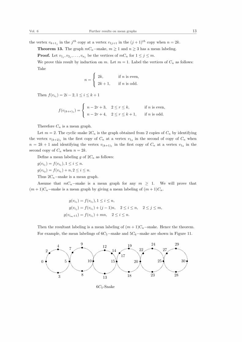
Theorem 13. The graph mCn−snake, m ≥ 1 and n ≥ 3 has a mean labeling.
Proof. Let v1j, v2j
, . . . , vnjbe the vertices of mCn for 1 ≤ j ≤ m.
We prove this result by induction on m. Let m = 1. Label the vertices of Cn as follows:
Take
n =
2k, if n is even,
2k + 1, if n is odd.
Then f(vi1) = 2i− 2, 1 ≤ i ≤ k + 1
f(v(k+r)1) =
n− 2r + 3, 2 ≤ r ≤ k, if n is even,
n− 2r + 4, 2 ≤ r ≤ k + 1, if n is odd.
Therefore Cn is a mean graph.
Let m = 2. The cyclic snake 2Cn is the graph obtained from 2 copies of Cn by identifyingthe vertex v(k+2)1 in the first copy of Cn at a vertex v12 in the second of copy of Cn whenn = 2k + 1 and identifying the vertex v(k+1)1 in the first copy of Cn at a vertex v12 in thesecond copy of Cn when n = 2k.
Define a mean labeling g of 2Cn as follows:
g(vi1) = f(vi1), 1 ≤ i ≤ n.
g(vi2) = f(vi1) + n, 2 ≤ i ≤ n.
Thus 2Cn−snake is a mean graph.
Assume that mCn−snake is a mean graph for any m ≥ 1. We will prove that(m + 1)Cn−snake is a mean graph by giving a mean labeling of (m + 1)Cn.
g(vi1) = f(vi1), 1 ≤ i ≤ n,
g(vij) = f(vi1) + (j − 1)n, 2 ≤ i ≤ n, 2 ≤ j ≤ m,
g(vim+1) = f(vi1) + mn, 2 ≤ i ≤ n.
Then the resultant labeling is a mean labeling of (m + 1)Cn−snake. Hence the theorem.
For example, the mean labelings of 6C5−snake and 5C6−snake are shown in Figure 11.
s
s
s
s
s
s
s
s
s
s
s s s s s ssss
6C5-Snake
0
3
5
47
9
10
8
12
15
13
s1417
19
20
18
2224
25
23
s
s
ss27
29
30
28
s2

14 R. Vasuki and A. Nagarajan No. 3
s
s
s
s
s
s
s
s
s
s
s ss
s s s sss
s
s
5C6-Snake
0 6
4
53
s
s
s
s s
2
10
12
119
8 1416
18
17
15
2022
24
2321
2628
30
2927
Figure 11.
References
[1] R. Balakrishnan and N. Renganathan, A Text Book on Graph Theory, Springer Verlag,2000.
[2] R. Ponraj and S. Somasundaram, Further results on mean graphs, Proceedings of Sacoef-erence, 2005, 443-448.
[3] Selvam Avadayappan and R. Vasuki, Some results on mean graphs, Ultra Scientist ofPhysical Sciences, 21(2009), No. 1, 273-284.
[4] S. Somasundaram and R. Ponraj, Mean labelings of graphs, National Academy Scienceletter, 26(2003), 210-213.
[5] S. Somasundaram and R. Ponraj, On Mean graphs of order ≤ 5, Journal of Decisionand Mathematical Sciecnes, 9(2004), No. 1-3, 48-58.
[6] A. Nagarajan and R. Vasuki, Meanness of the graphs Pa,b and P ba , International Journal
of Applied Mathematics, 22(2009), No. 4, 663-675.
Scientia MagnaVol. 6 (2010), No. 3, 15-19
A short interval result for the exponentialdivisor function
Shuqian Gao† and Qian Zheng‡
School of Mathematical Sciences, Shandong Normal University,Jinan 250014, China
E-mail: [email protected] [email protected]
Abstract An integer d =∏s
i=1 pbii is called the exponential divisor of n =
∏si=1 pai
i > 1 if
bi|ai for every i ∈ 1, 2, · · · , s. Let τ (e)(n) denote the number of exponential divisors of n,
where τ (e)(1) = 1 by convention. The aim of this paper is to establish a short interval result
for −r-th power of the function τ (e) for any fixed integer r ≥ 1.
Keywords The exponential divisor function, arithmetic function, short interval.
§1. Introduction
Let n > 1 be an integer of canonical from n =∏s
i=1 paii . An integer d =
∏si=1 pbi
i is calledthe exponential divisor of n if bi|ai for every i ∈ 1, 2, · · · , s, notation: d|en. By convention1|e1.
Let τ (e)(n) denote the number of exponential divisors of n. The function τ (e) is calledthe exponential divisor function. The properties of the function τ (e) is investigated by severalauthors (see for example [1], [2], [3]).
Let r ≥ 1 be a fixed integer and define Qr(x) :=∑
n≤x(τ (e)(n))−r. Recently ChenghuaZheng [5] proved that the asymptotic formula
Qr(x) = Arx + x12 log2−r−2(
N∑
j=0
dj(r)log−j x + O(log−N−1 x)) (1)
holds for any fixed integer N ≥ 1, where d0(r), d1(r), · · · , dN (r) are computable constants, and
Ar :=∏p
(1 +∞∑
a=2
(τ(a))−r − (τ(a− 1))−r
pa). (2)
The aim of this short note is to study the short interval case and prove the following.Theorem. If x
15+2ε ≤ y ≤ x, then
∑
x<n≤x+y
(τ (e)(n))−r = Ary + (yx−ε2 + x
15+ 3ε
2 ), (3)
where Ar is given by (2).

16 Shuqian Gao and Qian Zheng No. 3
Throughout this paper, ε always denotes a fixed but sufficiently small positive constant.Suppose that 1 ≤ a ≤ b are fixed integers, the divisor function d(a, b; k) is defined by
d(a, b; k) =∑
k=na1nb
2
1.
The estimate d(a, b; k) ¿ kε2 will be used freely. For any fixed z ∈ C, ζz(s)(<s > 1) is definedby exp(z log ζ(s)) such that log 1 = 0.
§2. Proof of the theorem
Lemma 1. Suppose s is a complex number (<s > 1), then
F (s) :=∞∑
n=1
(τ (e)(n))−r
ns= ζ(s)ζ2−r−1(2s)ζ−cr (4s)M(s),
where cr = 2−r−1 + 2−2r−1− 3−r > 0 and the Dirichlet series M(s) :=∑∞
n=1g(n)ns is absolutely
convergent for <s > 1/5.Proof. Here τ (e)(n) is multiplicative and by Euler product formula we have for σ > 1
that,
∞∑n=1
(τ (e)(n)
ns) =
∏p
(1 +(τ (e)(p))−r
ps+
(τ (e)(p2))−r
p2s+
(τ (e)(p3))−r
p3s+ · · · ) (1)
=∏p
(1 +1ps
+2−r
p2s+
2−r
p3s+
3−r
p4s· · · )
=∏p
(1− 1ps
)−1∏p
(1− 1ps
)(1 +1ps
+2−r
p2s+
2−r
p3s· · · )
= ζ(s)ζ2−r−1(2s)∏p
(1− 1ps
)2−r−1(1 +
2−r − 1p2s
+3−r − 2−r
p4s+ · · · )
= ζ(s)ζ2−r−1(2s)ζ−cr (4s)M(s).
So we get cr = 2−r−1+2−2r−1−3−r and M(s) :=∑∞
n=1g(n)ns . By the properties of Dirichlet
series, the later one is absolutely convergent for Res > 1/5.Lemma 2. Let k ≥ 2 be a fixed integer, 1 < y ≤ x be large real numbers and
B(x, y; k, ε) :=∑
x < nmk ≤ x + y
m > xε
1.
Then we haveB(x, y; k, ε) ¿ yx−ε + x
12k+1 log x.
Proof. This is just a result of k-free number [4].Let a(n), b(n), c(n) be arithmetic functions defined by the following Dirichlet series (for
<s > 1),

Vol. 6 A short interval result for the exponential divisor function 17
∞∑n=1
a(n)ns
= ζ(s)M(s), (2)
∞∑n=1
b(n)ns
= ζ2−r−1(s), (3)
∞∑n=1
c(n)ns
= ζ−cr (s). (4)
Lemma 3. Let a(n) be an arithmetic function defined by (2), then we have
∑
n≤x
a(n) = A1x + O(x15+ε), (5)
where A1 = Ress=1ζ(s)M(s).
Proof. Using Lemma 1, it is easy to see that
∑
n≤x
|g(n)| ¿ x15+ε.
Therefore from the definition of g(n) and (2), it follows that
∑
n≤x
a(n) =∑
mn≤x
g(n) =∑
n≤x
g(n)∑
m≤ xn
1
=∑
n≤x
g(n)(x
n+ O(1)) = A1x + O(x
15+ε),
and A1 = Ress=1ζ(s)M(s).
Now we prove our Theorem. From Lemma 3 and the definition of a(n), b(n), c(n), we get
(τ (e)(n))−r =∑
n=n1n22n4
3
a(n1)b(n2)c(n3),
and
a(n) ¿ nε2 , b(n) ¿ nε2 , c(n) ¿ nε2 . (6)
So we have
Qr(x + y)−Qr(x) =∑
x<n1n22n4
3≤x+y
a(n1)b(n2)c(n3)
=∑1
+O(∑2
+∑3
), (7)

18 Shuqian Gao and Qian Zheng No. 3
where∑1
=∑
n2 ≤ xε
n3 ≤ xε
b(n2)c(n3)∑
x
n22n4
3<n1≤ x+y
n22n4
3
a(n1),
∑2
=∑
x < n1n22n4
3 ≤ x + y
n2 > xε
|a(n1)b(n2)c(n3)|,
∑3
=∑
x < n1n22n4
3 ≤ x + y
n3 > xε
|a(n1)b(n2)c(n3)|.
(8)
By Lemma 3 we get
∑1
=∑
n2 ≤ xε
n3 ≤ xε
b(n2)c(n3)(A1y
n22n
43
+ O((x
n22n
43
)15+ε))
= Ary + O(yx−ε2 + x
15+ 3
2 ε), (9)
where Ar = Ress=1F (s). For Σ2 we have by Lemma 2 and (6) that∑2
¿∑
x < n1n22n4
3 ≤ x + y
n2 > xε
(n1n2n3)ε2
¿ xε2∑
x < n1n22n4
3 ≤ x + y
n2 > xε
1
= xε2∑
x < n1n22 ≤ x + y
n2 > xε
d(1, 4;n1)
¿ x2ε2B(x, y; 2, ε)
¿ x2ε2(yx−ε + x15+ε)
¿ yx2ε2−ε + x15+ 3
2 ε log x
¿ yx−ε2 + x
15+ 3
2 ε, (10)
if ε < 1/4.
Similarly we have ∑3
¿ yx−ε2 + x
15+ 3
2 ε. (11)
Now our theorem follows from (7)-(11).
References
[1] J. Wu, Probleme de diviseeurs et entiers exponentiellement sans factor carre. J. Theor.Nombres Bordeaux, 7(1995), 133-141.
Vol. 6 A short interval result for the exponential divisor function 19
[2] M. V. Subbaro, On some arithmetic convolutions, In The Theory of Arithmetic Func-tions, Lecture Notes in Mathematic, pringer, 251(1972), 247-271.
[3] E. Kratzel, Lattice points, Kluwer, Dordrecht-Boston-London, 1988.[4] M. Filaseta, O. Trifonov, The distribution of square full numbers in short intervals,
Acta Arith., 67(1994), 323-333.[5] Chenghua Zheng and Lixia Li, A negative order result for the exponential divisor
function, Scientia Magna, 5(2009), 85-90.

Scientia MagnaVol. 6 (2010), No. 3, 20-24
On the mean value of some new sequences 1
Chan Shi
Department of Mathematics, Northwest University, Xi’an, Shaanxi, P.R.China
Abstract The main purpose of this paper is to studied the mean value properties of some
new sequences, and give several mean value formulae and their applications.
Keywords New sequences, mean value, asymptotic formula, applications.
§1. Introduction
For any monotonous increasing arithmetical function g(n), we define two sequences h(n)and f(n) as follows: h(n) is defined as the smallest positive integer k such that g(k) greaterthan or equal to n. That is, h(n) = mink : g(k) ≥ n. f(n) is defined as the largest positiveinteger k such that g(k) less than or equal to n. That is, f(n) = maxk : g(k) ≤ n. Furthermore, we let
Sn = (h(1) + h(2) + · · ·+ h(n))/n;
In = (f(1) + f(2) + · · ·+ f(n))/n;
Kn = n√
h(1) + h(2) + · · ·+ h(n);
Ln = n√
f(1) + f(2) + · · ·+ f(n).
In references [1], Dr. Kenichiro Kashihara asked us to studied the properties of In, Sn, Kn
and Ln. In references [3] and [4], Gou Su and Wang Yiren studied this problem, and obtainedsome interesting results. In this paper, we will use the elementary and analytic methods tostudy some similar problems, and prove a general result. As some applications of our theorem,we also give two interesting asymptotic formulae. That is, we shall prove the following:
Theorem. For any positive integer k, let g(k) > 0 be an increasing function, we have
Sn − In =1n
(∫ M
M−1
g(t) dt +∫ M
M−1
(t− [t]) g′(t) dt + O(M)
),
Sn
In=
1n
(Mx− ∫ M−1
0g(t) dt− ∫ M−1
0(t− [t]) g′(t) dt + O (M)
Mx− ∫ M
1g(t) dt− ∫ M
1(t− [t]) g′(t) dt + O (M)
),
and
Kn
Ln=
(Mx− ∫ M−1
0g(t) dt− ∫ M−1
0(t− [t]) g′(t) dt + O (M)
Mx− ∫ M
1g(t) dt− ∫ M
1(t− [t]) g′(t) dt + O (M)
) 1n
.
1This paper is supported by the N. S. F. of P.R.China.

Vol. 6 On the mean value of some new sequences 21
As some applications of our theorem, we shall give two interesting examples. First wetaking g(k) = km, that is h(n) = mink : km ≥ n and f(n) = maxk : km ≤ n. Then wehave
Corollary 1. Let g(k) = km, then for any positive integer n, we have the asymptoticformulae
Sn − In = 1 + O(n−
1m
),
Sn
In= 1 + O
(n−
1m
),
and
Kn
Ln= 1 + O
(1n
), lim
n→∞Sn
In= 1, lim
n→∞Kn
Ln= 1.
Next, we taking g(k) = ek, that is h(n) = mink : ek ≥ n and f(n) = maxk : ek ≤ n,then we have:
Corollary 2. Let g(k) = ek, then for any positive integer n, we have the asymptoticformulae
Sn
In= 1 + O
(1
lnn
),
Kn
Ln= 1 + O
(1n
),
limn→∞
Sn
In= 1, lim
n→∞Kn
Ln= 1.
§2. Proof of the theorem
In this section, we shall use the Euler summation formula and elementary method tocomplete the proof of our theorem. For any real number x > 2, it is clear that there exists oneand only one positive integer M such that g(M) < x < g(M + 1). So we have
∑
n≤x
h(n) =M∑
k=1
∑
g(k−1)≤n<g(k)
h(n) +∑
g(M)<n≤x
h(n)
=∑
g(0)≤n<g(1)
h(n) +∑
g(1)≤n<g(2)
h(n) + · · ·+∑
g(M)≤n<x
h(n)
=M∑
k=1
k(g(k)− g(k − 1)) + M (x− g(M)) + O (M)
= Mg(M)−M−1∑
k=0
g(k) + M (x− g(M)) + O (M)
= Mx−∫ M−1
0
g(t) dt−∫ M−1
0
(t− [t]) g′(t) dt + O (M) , (1)

22 Chan Shi No. 3
and
∑
n≤x
f(n) =M∑
k=1
∑
g(k)<n≤g(k+1)
f(n)−∑
x<n≤g(M+1)
f(n)
=∑
g(1)<n≤g(2)
f(n) +∑
g(2)<n≤g(3)
f(n) + · · ·+∑
g(M)<n≤g(M+1)
f(n)
−M (g (M + 1)− x)
=M∑
k=1
k(g(k + 1)− g(k))−M (g (M + 1)− x)
= (M + 1)g(M + 1)−M+1∑
k=2
g(k)−M (g (M + 1)− x)
= Mx−∫ M
1
g(t) dt−∫ M
1
(t− [t]) g′(t) dt + O (M) . (2)
In order to prove our theorem, we taking x = n in (1) and (2), by using the elementary methodwe can get
Sn − In =1n
(h(1) + h(2) + · · ·+ h(n))− 1n
(f(1) + f(2) + · · ·+ f(n))
=1n
(∫ M
M−1
g(t) dt +∫ M
M−1
(t− [t]) g′(t) dt + O(M)
). (3)
Then we have
Sn
In=
Mx− ∫ M−1
0g(t) dt− ∫ M−1
0(t− [t]) g′(t) dt + O (M)
Mx− ∫ M
1g(t) dt− ∫ M
1(t− [t]) g′(t) dt + O (M)
,
and
Kn
Ln=
(Mx− ∫ M−1
0g(t) dt− ∫ M−1
0(t− [t]) g′(t) dt + O (M)
Mx− ∫ M
1g(t) dt− ∫ M
1(t− [t]) g′(t) dt + O (M)
) 1n
.
This completes the proof of our theorem.Now we prove Corollary 1. Taking g(k) = km in our theorem, for any real number x > 2,
it is clear that there exists one and only one positive integer M satisfying Mm < x < (M +1)m.That is, M = x
1m + O(1). So from our theorem we have
∑
n≤x
h(n) =M∑
k=1
∑
(k−1)m≤n<km
h(n) +∑
Mm<n≤x
h(n)
= Mx−∫ M−1
0
tm dt−∫ M−1
0
(t− [t]) (tm)′ dt + O (M)
= Mx− 1m + 1
(M − 1)m+1 + O (Mm) .
Since M = x1m + O(1), so we have the asymptotic formula
∑
n≤x
h(n) =m
m + 1x
m+1m + O(x).

Vol. 6 On the mean value of some new sequences 23
Similarly, we have∑
n≤x
f(n) = Mx−∫ M
1
g(t) dt−∫ M
1
(t− [t]) g′(t) dt + O (M)
= Mx− 1m + 1
(M − 1)m+1 + O (Mm)
=m
m + 1x
m+1m + O(x).
On the other hand, we also have
Sn − In =1n
(∫ M
M−1
g(t) dt +∫ M
M−1
(t− [t]) g′(t) dt + O(M)
)
=1n
Mm + O
(M
n
)= 1 + O
(n−
1m
).
Sn
In=
Mx− ∫ M−1
0tm dt− ∫ M−1
0(t− [t]) (tm)′ dt + O (M)
Mx− ∫ M
1tm dt− ∫ M
1(t− [t]) (tm)′ dt + O (M)
=m
m+1nm+1
m + O(n)m
m+1nm+1
m + O(n)= 1 + O
(n−
1m
).
Kn
Ln=
(m
m+1nm+1
m + O(n)m
m+1nm+1
m + O(n)
) 1n
= 1 + O
(1n
).
limn→∞
Sn
In= 1, lim
n→∞Kn
Ln= 1.
Now we prove Corollary 2. Taking g(k) = ek in our theorem. For any real number x > 2,it is clear that there exists one and only one positive integer M satisfying eM < x < eM+1,that is M = ln x + O(1). Then
∑
n≤x
h(n) = Mx−∫ M−1
0
et dt−∫ M−1
0
(t− [t]) (et)′ dt + O (lnx) ,
and∑
n≤x
f(n) = Mx−∫ M
1
et dt−∫ M
1
(t− [t]) (et)′ dt + O (lnx) .
Therefore,
Sn
In=
Mx− ∫ M−1
0et dt− ∫ M−1
0(t− [t]) (et)′ dt + O (lnx)
Mx− ∫ M
1et dt− ∫ M
1(t− [t]) (et)′ dt + O (lnx)
= 1 + O
(1
lnn
),
Kn
Ln=
(1 + O
(1
lnn
)) 1n
= 1 + O
(1n
),
and
limn→∞
Sn
In= 1, lim
n→∞Kn
Ln= 1.
This completes the proof of our corollaries.

24 Chan Shi No. 3
References
[1] Kenichiro Kashihara, Comments and topics on Smarandache notions and problems,Erhus University Press, USA, 1996.
[2] F. Smarandache, Only Problems, Not Solutions, Chicago, Xiquan Publishing House,1993.
[3] Wang Yiren, On the mean value of SSMP (n) and SIMP (n), Scientia Magna, 5(2009),No. 3, 1-5.
[4] Gou Su, On the mean values of SSSP (n) and SISP (n), Pure and Applied Mathematics,25(2009), No. 3, 431-434.
[5] Du Fengying, On a conjecture of the Smarandache function S(n), 23(2007), No. 2,205-208.
[6] Zhang Wenpeng, The elementary number theory (in Chinese), Shaanxi Normal Univer-sity Press, Xi’an, 2007.

Scientia MagnaVol. 6 (2010), No. 3, 25-28
A short interval result for the exponentialMobius function
Qian Zheng† and Shuqian Gao‡
School of Mathematical Sciences, Shandong Normal University,Jinan 250014, China
E-mail: [email protected] [email protected]
Abstract The integer d =∏s
i=1 pbii is called an exponential divisor of n =
∏si=1 pai
i > 1 if
bi|ai for every i ∈ 1, 2, · · · , s. The exponential convolution of aithmetic functions is defined
by
(f⊙
g)(n) =∑
b1c1=a1
· · ·∑
brcr=ar
= f(pb11 · · · pbr
r )g(pc11 · · · pcr
r ),
where n =∏s
i=1 paii . The inverse of the constant function with respect to
⊙is called the
exponential analogue of the Mobius function, which is denoted by µ(e). The aim of this paper
is to establish a short interval result for the function µ(e).
Keywords The exponential divisor function, generalized divisor function, short interval.
§1. Introduction
Let n > 1 be an integer of canonical from n =∏s
i=1 paii . The integer n =
∏si=1 pbi
i is calledan exponential divisor of n if bi|ai for every i ∈ 1, 2, · · · , s, notation: d|en. By convention1|e1.
Let µ(e)(n) = µ(a1) · · ·µ(ar) here n =∏s
i=1 paii . Observe that |µ(e)| = 0 or |µ(e)| = 1,
according as n is e-squarefree or not. The properties of the function µ(e) is investigated bymany authors. An asymptotic fomula for A(x) :=
∑n≤x µ(e)(n) was established by M. V.
Subarao [2] and improved by J. Wu [1]. Recently Laszlo Toth [3] proved that
A(x) = m(µe)x + O(x12 exp(−c(log x)∆), (1)
where
m(µe) :=∏p
(1 +p∑
a=2
(µ(a)− µ(a− 1))pa
), (2)
and 0 < ∆ < 9/25 and c > 0 are fixed constants.The aim of this paper is to study the short interval case and prove the followingTheorem. If x
15+ 3
2 ε ≤ y ≤ x, then∑
x<n≤x+y
µ(e)(n) = m(µe)y + O(yx−12 ε + x
15+ 3
2 ε),
where m(µe) is given by (2).

26 Qian Zheng and Shuqian Gao No. 3
Notation. Throughout this paper, ε denotes a sufficiently small positive constant. µ(n)denotes the Mobius function. For fixed integers 1 ≤ a ≤ b, the divisor function d(a, b;n) isdefined by
d(a, b;n) :=∑
n=na1nb
2
1.
§2. Proof of the theorem
Lemma 1. Suppose <s > 1, then we have
F (s) :=∞∑
n=1
µ(e)(n)ns
=ζ(s)
ζ2(2s)ζ(5s)G(s), (1)
where the Dirichlet series G(s) :=∞∑
n=1
g(n)ns
is absolutely convergent for Res > 1/5.
Proof. Since µ(e)(n) is multiplicative, by Euler product formula we get for σ > 1 that
∞∑n=1
µ(e)(n)ns
=∏p
(1 +µ(1)ps
+µ(2)p2s
+µ(3)p3s
+ · · · )
=∏p
(1− 1ps
)−1∏p
(1− 1ps
)(1 +1ps− 1
p2s− 1
p3s+ · · · )
= ζ(s)∏p
(1− 2p2s
+1
p4s− 1
p5s+ · · · )
= ζ(s)∏p
(1− 2p2s
+1
p4s− 1
p5s+ · · · )
=ζ(s)
ζ2(2s)ζ(5s)
∏p
(1 +2
p6s − ps− 4
p7s − p2s+
5p8s − p3s
+ · · · )
=ζ(s)
ζ2(2s)ζ(5s)G(s),
where
G(s) =∏p
(1 +2
p6s − ps− 4
p7s − p2s+
5p8s − p3s
+ · · · ).
It is easily seen that G(s) can be written as a Dirichlet series, which is absolutely convergentfor <s > 1/5.
Lemma 2. Let k ≥ 2 be a fixed integer, 1 < y ≤ x be large real numbers and
B(x, y; k, ε) : =∑
x < nmk ≤ x + y
m > xε
1.
Then we have
B(x, y; k, ε) ¿ yx−ε + x1
2k+1 log x.
Proof. See [4].

Vol. 6 A short interval result for the exponential Mobius function 27
Let a(n), b(n) be arithmetic functions defined by the following Dirichlet series (for <s > 1),
∞∑n=1
a(n)ns
= ζ(s)G(s), (2)
∞∑n=1
b(n)ns
=1
ζ2(s). (3)
Lemma 3. Let a(n) be the arithmetic function defined by (2), then we have
∑
n≤x
a(n) = A1x + O(x15+ε), (4)
where A1 = Ress=1ζ(s)G(s).
Proof. According to Lemma 1, it is easy to see that
∑
n≤x
|g(n)| ¿ x15+ε.
Therefore from the definition of a(n) and g(n), it follows that
∑
n≤x
a(n) =∑
mn≤x
g(n) =∑
n≤x
g(n)∑
m≤ xn
1
=∑
n≤x
g(n)[x
n] = Ax + O(x
15+ε).
Now we prove our Theorem. From (1), the definitions of a(n) and b(n) we get that
µ(e)(n) =∑
n=n1n22n5
3
a(n1)b(n2)µ(n3),
thus
A(x + y)−A(x) =∑
x<n1n22n5
3≤x+y
a(n1)b(n2)µ(n3) (5)
=∑1
+O(∑2
+∑3
),
where
∑1
=∑
n2 ≤ xε
n3 ≤ xε
b(n2)µ(n3)∑
x
n22n5
3<n1≤ x+y
n22n5
3
a(n1),
∑2
=∑
x < n1n22n5
3 ≤ x + y
n2 > xε
|a(n1)b(n2)|,
∑3
=∑
x < n1n22n5
3 ≤ x + y
n3 > xε
|a(n1)b(n2)|.

28 Qian Zheng and Shuqian Gao No. 3
By Lemma 3 we get easily that
∑1
=∑
n2≤xε,n3≤xε
b(n2)µ(n3)(
A1y
n22n
53
+ O((x
n22n
53
)15+ε))
)(6)
= A1y∑
n2≤xε
b(n2)n−22
∑
n3≤xε
µ(n3)n−53 + O(x
15+ 3
2 ε))
= Ay + O(yx−ε + x15+ 3
2 ε),
where A = Ress=1F (s) = m(µe).It is easily seen that the estimates
a(n) ¿ nε2 ,
andb(n) =
∑
n=n21n2
2
µ(n1)µ(n2) ¿ d(1, 1;n) ¿ nε2 ,
hold, which combining the estimate d(1, 5;n) ¿ nε2 and Lemma 2 gives∑2
¿∑
x<n1n22n5
3≤x+y
(n1n22)
ε2 (7)
¿ xε2∑
x<n1n22n5
3≤x+y
1
¿ x2ε2∑
x<n1n22≤x+y
d(1, 5;n1)
¿ x2ε2(yx−ε + x15+ε)
¿ yx−ε2 + x
15+ 3
2 ε.
Similay we have ∑3
¿ yx−ε2 + x
15+ 3
2 ε. (8)
Now our theorem follows from (5)-(8).
References
[1] J. Wu, Probleme de diviseeurs et entiers exponentiellement sans factor carre. J. Theor.Numbers Bordeaux, 7(1995), 133-141.
[2] M. V. Subbaro, On some arithmetic convolutions, in The Theory of Arithmetic Func-tions, Lecture Notes in Mathematic, Springer, 251(1972), 247-271.
[3] Laszlo Toth, On certain arithmetic fuctions involving exponential divisos,∏
AnalsUniv. Sci. udapst, Sect. Comp., 27(2007), 155-166.
[4] Wenguang Zhai, Square-free integers as sums of two squares, Number Theory: Taditionand modernization, Springer, New York, 2006, 219-227.

Scientia MagnaVol. 6 (2010), No. 3, 29-33
Approach of wavelet estimation in a
semi-parametric regression model withρ-mixing errors1
Wei Liu† and Zhenhai Chang‡
School of Mathematics and Statistics, Tianshui Normal University,Tianshui, Gansu 741000, P.R.China
E-mail: [email protected]
Abstract Consider the wavelet estimator of a semi-parametric regression model with fixed
design points when errors are a stationary ρ-mixing sequence. The wavelet estimators of
unknown parameter and non-parameter are derived by the wavelet method. Under proper
conditions, weak convergence rates of the estimators are obtained.
Keywords Semi-parametric regression model, wavelet estimator, ρ-mixing, convergence
rate.
§1. Introduction
Consider a semi-parametric regression model
yi = xiβ + g(ti) + ei, i = 1, 2, · · · , n. (1)
where xi ∈ R1, ti ∈ [0, 1], (xi, ti), 1 ≤ i ≤ n is a deterministic design sequence, β is anunknown regression parameter, g(·) is an unknown Borel function, the unobserved processei, 1 ≤ i ≤ n is a stationary ρ-mixing sequence and satisfies Eei = 0, i = 1, 2, · · · , n.
In recent years, the parametric or non-parametric estimators in the semi-parametric ornon-parametric regression model have been widely studied in the literature when errors area stationary mixing sequence (example [1]-[4]). But up to now, the discussion of the waveletestimators in the semi-parametric regression model, whose errors are a stationary ρ-mixingsequence, has been scarcely seen.
Wavelets techniques, due to their ability to adapt to local features of curves, have recentlyreceived much attention from mathematicians, engineers and statisticians. Many authors haveapplied wavelet procedures to estimate nonparametric and semi-parametric models ([5]-[7]).
In this article, we establish weak convergence rates of the wavelet estimators in the semi-parametric regression model with ρ-mixing errors, which enrich existing estimation theories andmethods for semi-parametric regression models.
Writing wavelet scaling function φ(·) ∈ Sq (q-order Schwartz space), multiscale analysis of

30 Wei Liu and Zhenhai Chang No. 3
concomitant with L2(R) is Vm. And reproducing wavelet kernel of Vm is
Em(t, s) = 2mE0(2mt, 2ms) = 2m∑
k∈Z
ϕ(2mt− k)ϕ(2ms− k).
When β is known, we define the estimator of g(·),
g0(t, β) =n∑
i=1
(yi − xiβ)∫
Ai
Em(t, s)ds.
where Ai = [si−1, si] is a partition of interval [0, 1] with ti ∈ Ai, 1 ≤ i ≤ n. Then, we solve the
minimum problem minβ∈R
n∑i=1
(yi − xiβ − g0(t, β))2. Let its resolution be βn, we have
βn = S−2n
n∑
i=1
xiyi. (2)
where xi = xi −n∑
j=1
xj
∫Aj
Em(ti, s)ds, yi = yi −n∑
j=1
yj
∫Aj
Em(ti, s)ds, S2n =
n∑i=1
x2i .
Finally, we can define the estimator of g(·),
g(t) , g0(t, βn) =n∑
i=1
(yi − xiβn)∫
Ai
Em(t, s)ds. (3)
§2. Assumption and lemmas
We assume that C and Ci, i ≥ 1 express absolute constant, and they can express differentvalues in different places.
2.1. Basic assumption
(A1) g(·) ∈ Hυ(υ > 1/2) satisfies γ-order Lipschitz condition.(A2) φ has compact support set and is a q-regular function.(A3)
∣∣∣φ(ξ)− 1∣∣∣ = φ(ξ), ξ → 0, where φ is Fourier transformation of φ.
(A4) max1≤i≤n
(si − si−1) = O(n−1), max1≤i≤n
|xi| = O(2m).
(A5) C1 ≤ S2n/n ≤ C2, where n is large enough.
(A6) |n∑
i=1
xi
∫Ai
Em(t, s)ds| = λ, t ∈ [0, 1], where λ is a constant that depends only on t.
2.2. Lemmas
Lemma 1.[8] Let φ(·) ∈ Sq. Under basic assumptions of (A1)-(A3), if for each integerk ≥ 1, ∃ck > 0, such that
(i) |E0(t, s)| ≤ ck
1 + |t− s|k, |Em(t, s)| ≤ 2mck
1 + 2m |t− s|k;
(ii) supt,m
∫ 1
0|Em(t, s)|ds ≤ C.
Lemma 2.[3] Under basic assumption (A1)-(A4), we have

Vol. 6Approach of wavelet estimation in a semi-parametric
regression model with ρ-mixing errors 31
(i)∣∣∣∫
AiEm(t, s)ds
∣∣∣ = O( 2m
n );
(ii)n∑i
(∫
AiEm(t, s)ds)2 = O( 2m
n ).
Lemma 3.[3] Under basic assumption (A1)-(A5), we have
supt
∣∣∣∣∣n∑
i=1
g(ti)∫
Ai
Em(t, s)ds− g(t)
∣∣∣∣∣ = O(n−γ) + O(τm), n →∞.
where
τm =
(2m)−α+1/2, (1/2 < α < 3/2),√
m/2m, (α = 3/2),
1/2m, (α > 3/2).
Lemma 4.[9] (Bernstein inequality) Let xi, i ∈ N be a ρ-mixing sequence and E|xi| =
0. ani, 1 ≤ i ≤ n is a constant number sequence. xi ≤ di, a.s.. sn =n∑
i=1
anixi, then for
∀ε > 0, such that
P (|sn| > ε) ≤ C1 exp−tε + 2C2t
2∆ + 2(l + 1) + 2 ln(ρ(k))
.
where constant C1 do not depend on n, and C2 = 2(1+2δ)(1+8∞∑
i=1
ρ(i)), ∆ =∞∑
i=1
a2nid
2i , t > 0.
l and k satisfy the following inequality
2lk ≤ n ≤ 2(l + 1)k, tk · max1≤i≤n
|anidi| ≤ δ ≤ 12.
§3. Main results and proofs
Theorem 1. Under basic assumption (A1)-(A6), if∞∑
i=1
ρ(i) < ∞, Λn = max(n−γ , τm),
and if ∃ d = d(n) ∈ N, such that dΛn →∞,n
d2Λn→ 0 and
2md3
nΛn→ 0,
then, we haveβn − β = Op(Λn), (4)
g(t)− g(t) = Op(Λn). (5)
Proof. It is obvious that
βn − β = S−2n (
n∑i=1
xiei +n∑
i=1
xigi)
= S−2n [
n∑i=1
xiei −n∑
i=1
xi
n∑j=1
ej
∫Aj
Em(ti, s)ds +n∑
i=1
xigi]
∆= B1n + B2n + B3n,
(6)
where ei = ei −n∑
j=1
ej
∫Aj
Em(ti, s)ds, gi = gi −n∑
j=1
gj
∫Aj
Em(ti, s)ds.
Since |B1n| =∣∣∣∣
n∑i=1
S−2n xiei
∣∣∣∣∆=
∣∣∣∣n∑
i=1
biei
∣∣∣∣ .
32 Wei Liu and Zhenhai Chang No. 3
Hence
P (|B1n| > ηΛn) = P (∣∣∣∣
n∑i=1
biei
∣∣∣∣ > ηΛn)
≤ P (∣∣∣∣
n∑i=1
bieiI(|ei| ≤ d)∣∣∣∣ > ηΛn) + P (
∣∣∣∣n∑
i=1
bieiI(|ei| > d)∣∣∣∣ > ηΛn)
∆= P (Jn1) + P (Jn2),
(7)
where d = d(n) ∈ N.
By assumption (A4) and (A5), we have
|bi| =∣∣∣S−2
n xi
∣∣∣ = O
(2m
n
),
n∑
i=1
b2i =
n∑
i=1
(S−2n xi)2b2
i ≤ maxi
S−2n xi ·
n∑
i=1
S−2n xi = O
(2m
n
).
If further d = t = k in Lemma 4, then the conditions of Lemma 4 suffice.By applying Markov’s inequality and the conditions of Theorem 1, we have
P (Jn2) ≤E(
∣∣∣∣n∑
i=1
bieiI(|ei| > d)∣∣∣∣)
ηΛn≤
Ee2i ·
n∑i=1
bi
dηΛn=
Ee2i ·
n∑i=1
(n−1xi) · (ns−2n )
dηΛn≤ C
dΛn→ 0. (8)
By Lemma 4, we have
P (Jn1) ≤ C1 exp−tΛnη + C2t
2∆ + 2(l + 1) + 2 ln(ρ(k))
≤ C1 exp−dΛnη + C2d
2∆ + 2(l + 1)
.
Since
∆ =n∑
i=1
b2i d
2 =2md2
n,
Sod2∆dΛn
=2md3
nΛn→ 0,
l + 1dΛn
≤ n/2k + 1dΛn
=n + 2d
2d2Λn=
n
2d2Λn+
1dΛn
→ 0.
Therefore(l + 1) + d2∆
dΛn→ 0.
Hence
P (Jn1) ≤ C1 · exp−d
2Λnη
→ 0 (d →∞). (9)
Thus, we have shownB1n → op(Λn). (10)
Write bj =n∑
i=1
S−2n xi
∫Aj
Em(ti, s)ds.
Then |B2n| = |n∑
j=1
bjej |.Note that
|bj | ≤n∑
i=1
S−2n xi ·max
i
∫
Aj
Em(ti, s)ds = nS−2n · n−1
n∑
i=1
xi ·maxi
∫
Aj
Em(ti, s)ds = O(2m
n),
n∑
j=1
b2j =
n∑
j=1
(n∑
i=1
S−2n xi
∫
Aj
Em(ti, s)ds)2 ≤n∑
i=1
(S−2n xi)2 ·max
i
n∑
j=1
∫
Aj
Em(ti, s)ds ≤ C · 22m
n2.
Vol. 6Approach of wavelet estimation in a semi-parametric
regression model with ρ-mixing errors 33
Similarly to the proof of B1n, we obtain
B2n → op(Λn). (11)
Consider now B3n. By assumption (A6) and Lemma 3, we have
|B3n| ≤ S−2n
n∑
i=1
|xi| · max1≤i≤n
|gi| = O(n−γ) + O(τm). (12)
Thus, by (6), (10), (11) and (12), the proof of (4) is completed.It is easy to see the following decompositions:
supt|g(t)− g(t)| ≤ sup
t|g0(t, β)− g(t)|+ sup
t
∣∣∣∣n∑
i=1
xi(β − βn)∫
AiEm(t, s)ds
∣∣∣∣≤ sup
t
∣∣∣∣n∑
i=1
g(ti)∫
AiEm(t, s)ds− g(t)
∣∣∣∣ + supt
∣∣∣∣n∑
i=1
ei
∫Ai
Em(t, s)ds
∣∣∣∣+
∣∣∣β − βn
∣∣∣ · supt
∣∣∣∣n∑
i=1
xi
∫Ai
Em(t, s)ds
∣∣∣∣∆= T1 + T2 + T3.
(13)
By Lemma 2, it is clear thatT1 = O(n−γ) + O(τm). (14)
Analogous to the proof of (4), and note that (13), (14) and (A6), it is clear that
g(t)− g(t) = Op(Λn).
References
[1] Wang S. R., Leng N. X., Strong consistency of wavelet estimation in the semi-parametricregression model, Journal of Hefei University of Technology, 32(2009), No. 1, 136-138.
[2] Li Y. M., Yin C. M. and Wei C. D., On the Asymptotic Normality for ϕ-mixingDependent Errors of Wavelet Regression Function Estimator, Acta Mathematicae ApplicataeSinica, 31(2008), No. 6, 1046-1055.
[3] Sun Y., Chai G. X., Non-parametric Estimation of a Fixed Designed Regression Func-tion, Acta Mathematica Scientia, 24A(2004), No. 5, 597-606.
[4] Xue L. G., Uniform Convergence Rates of the Wavelet Estimator of Regression FunctionUnder Mixing Error, Acta Mathematica Scientia, 22A(2002), No. 4, 528-535.
[5] Antoniadis A., Gregoire G., Mckeague I. W., Wavelet methods for curve estimation,Amer. Statist. Assoc, 89(1994), No. 5, 1340-1352.
[6] Qian W. M., Cai G. X., The strong convergence rate of Wavelet estimator in Partiallylinear models, Chinese Sci A, 29(1999), No. 4, 233-240.
[7] Li Y. M., Yang S. C., Zhou Y., Consistency and uniformly asymptotic normality ofwavelet estimator in regression model with assoeiated samples, Statist. Probab. Lett, 78(2008),No. 17, 2947-2956.
[8] Walter G. G., Wavelets and Other Orthogonal Systems with Applications, Florida, CRCPress, Inc, 1994.
[9] Chai Genxiang, Liu Jinyuan, Wavelet Estimation of Regression Function Based onMixing Sequence Under Fixed Design, Journal of Mathematical Research And Exposition,21(2001), No. 4, 555-560.

Scientia MagnaVol. 6 (2010), No. 3, 34-39
Generalize derivations on semiprime rings
Arkan. Nawzad†, Hiba Abdulla‡ and A. H. Majeed]
† Department of Mathematics, College of Science, Sulaimani University,Sulaimani-IRAQ
‡ ] Department of Mathematics, College of Science, Baghdad University,Baghdad-IRAQ
E-mail: hiba [email protected] [email protected]
Abstract The purpose of this paper is to study the concept of generalize derivations in the
sense of Nakajima on semi prime rings, we proved that a generalize Jordan derivation (f, ∂)
on a ring R is a generalize derivation if R is a commutative or a non commutative 2-torsion
free semi prime with ∂ is symmetric hochschilds 2-cocycles of R. Also we give a necessary
and sufficient condition for generalize derivations (f, ∂1), (g, ∂2) on a semi prime ring to be
orthogonal.
Keywords Prime ring, semi prime ring, generalize derivation, derivation, orthogonal deriva-
tion.
§1. Introduction
Throughout R will represent an associative ring with Z(R). R is said to be 2-torsion freeif 2x = 0, x ∈ R implies x = 0. As usual the commutator xy− yx will be denoted by [x, y]. Weshall use the basic commutator identites [xy, z] = [x, z]y+x[y, z] and is [x, yz] = y[x, y]+[x, y]z.Recall that a ring R is prime if aRb = 0 implies that either a = 0 or b = 0, and R is semiprime if aRa = 0 implies a = 0. An additive mapping d: R → R is called derivation ifd(ab) = d(a)b+ad(b) for all a, b ∈ R. And d is called Jordan derivation if d(a2) = d(a)a+ad(a)for all a ∈ R. In [3], M. Bresar introduced the definition of generalize derivation on rings asfollows: An additive map g: R → R is called a generalize derivation if there exists a derivationd: R → R such that g(ab) = g(a)b + ad(b) for all a, b ∈ R (we will call it of type 1). It isclear that every derivation is generalize derivation, and an additive map J : R → R is calledJordan generalize if there exists a derivation d: R → R such that J(a2) = J(a)a + ad(a) forall a ∈ R (we will call it of type 1). An additive map ∂: R × R → R be called hochschild2-cocylc if x(y, z) − ∂(xy, z) + ∂(x, yz) − ∂(x, y)z = 0 for all x, y, z ∈ R, the map ∂ is calledsymmetric if ∂(x, y) = ∂(y, x) for all x, y ∈ R. It is clear that every Jordan derivation is Jordangeneralize derivation, and every generalize derivation is Jordan generalize derivation, and sinceJordan derivation may be not derivation, so Jordan generalize derivation, may be not generalizederivation in general. The properties of this type of mapping were discussed in many papers([1],[2],[7]), especially, in [2], M. Ashraf and N. Rehman showed that if R is a 2-torsion freering which has a commtator non zero divisor, then every Jordan generalize derivation on R is
Vol. 6 Generalize derivations on semiprime rings 35
generalize derivation. In [7], Nurcan Argac, Atsushi Nakajima and Emine Albas introduced thenotion of orthogonality for a pair f, g of generalize derivation, and they gave several necessaryand sufficient conditions for f, g to be orthogonal. Nakajima [1] introduced another definition ofgeneralize derivation as following: An additive mapping f : R → R is called generalize derivationif there exist a 2 -coycle ∂: R×R→ R such that f(ab) = f(a)b+af(b)+∂(a, b) for all a, b ∈ R (wewill call it of type 2). And is called Jordan generalize derivation if f(a2) = f(a)a+af(a)+∂(a, a)for all a ∈ R (we will call it of type 2). In this paper we work on the generalize derivation (oftype 2), we will extend the result of ([1], Theorem 1) and also we give several sufficient andnecessary conditions which makes two generalize derivation (of type 2) to be orthogonal. For aring R, let U be a subset of R, then the left annihilator of U (rep, right annihilator of U) is theset a ∈ R such that aU = 0 (res, is the set a ∈ R such that Ua = 0). We denote the annihilatorof U by Ann(U). Note that U ∩Ann(U) = 0 and U ⊕Ann(U) is essential ideal of R.
§2. Preliminaries and examples
In this section, we give some examples and some well-known lemmas we are needed in ourwork.
Example 2.1. Let R be a ring d : R → R be a derivation and ∂ : R × R → R definedby ∂(a, b) = 2d(a)d(b) and g : R → R is defined as follows g(a) = d(d(a)) for all a ∈ R.g(a + b) = d(d(a + b)) = d(d(a) + d(b)) = d(d(a)) + d(d(b)) = g(a) + g(b) for all a, b ∈ R.
And, g(ab) = d(d(ab)) = d(d(a)b + ad(b)) = d(d(a)b) + d(ad(b)) = d(d(a))b + d(a)d(b) +d(a)d(b)+ ad(d(b)) = g(a)b+ ag(b)+2d(a)d(b) = g(a)b+ ag(b)+ ∂(a, b) for all a, b ∈ R. Hence,g is generalize derivation (of type 2) on R .
The following Example explains that the definition of generalize derivation (of type 2) ismore generalizing than the generalize derivation (of type 1).
Example 2.2. Let (f, d) be a generalize derivation on a ring R then the map (f, ∂) isgeneralize derivation, where ∂(a, b) = a(d− f)(b) for all a, b ∈ R.
Lemma 2.1.[5] Let R be a 2-torsion free ring, (f, ∂) : R → R be generalize Jordanderivation, then f(ab + ba) = f(ab) + f(ba) = f(a)b + af(b) + ∂(a, b) + f(b)a + bf(a) + ∂(b, a)for all a, b ∈ R.
Lemma 2.2.[5] Let R be a 2-torsion free ring and (f, ∂) : R → R be generalize Jordanderivation the map S: R×R → R defined as follows: S(a, b) = f(ab)− (f(a)b + af(b) + ∂(a, b)for all a, b ∈ R. And the map [ ] : R×R → R defined by [a, b] = ab− ba for all a, b ∈ R, thenthe following relations hold
(1) S(a, b)c[a, b] + [a, b]cS(a, b) = 0 for all a, b ∈ R.
(2) S(a, b)[a, b] = 0 for all a, b ∈ R.
Lemma 2.3. Let R be a 2-torsion free ring, (f, ∂) : R → R be generalize Jordan derivationthe map S : R × R → R defined as follows: S(a, b) = f(ab) − (f(a)b + af(b) + ∂(a, b)) for alla, b ∈ R, then the following relations hold
(1) S(a1 + a2, b)=S(a1, b) + S(a2, b) for all a1, a2, b ∈ R.
(2) S(a, b1 + b2)=S(a, b1) + S(a, b2) for all a, b1, b2 ∈ R.
36 Arkan. Nawzad, Hiba Abdulla and A. H. Majeed No. 3
Proof.
(1) S(a1 + a2, b) = f((a1 + a2)b)− (f(a1 + a2)b + (a1 + a2)f(b) + (a1 + a2, b))
= f(a1b) + f(a2b)− (f(a1)b + f(a2)b + a1f(b) + a2f(b)
+∂(a1, b) + ∂(a2, b))
= f(a1b)− (f(a1)b + a1f(b) + ∂(a1, b)) + f(a2b)− (f(a2)b
+a2f(b) + ∂(a2, b))
= S(a1, b) + S(a2, b).
(2) S(a, b1 + b2) = f(a(b1 + b2))− (f(a)(b1 + b2) + af(b1 + b2) + ∂(a, b1 + b2))
= f(ab1) + f(ab2)− (f(a))b1 + f(a)b2 + af(b1) + af(b2) +
∂(a, b1) + ∂(a, b2)
= f(ab1)− (f(a))b1 + af(b1) + ∂(a, b1) + f(ab2)− f(a)b2
+af(b2) + ∂(a, b2)
= S(a, b1) + S(a, b2).
Lemma 2.4.[1] If R is a 2-torsion free semi prime ring and a, b are elements in R then thefollowing are equivalent.
(i) a× b = 0 for all x in R.(ii) b× a = 0 for all x in R.(iii) a× b + b× a = 0 for all x in R. If one of them fulfilled, then ab = ba = 0.
§3. Generalize Jordan derivations on a semi prime rings
In this section, we extend the result proved by Nakajima ([1], Theorem 1(1), (2))by addingcondition.
Theorem 3.1. If R is a commutative 2-torsion free ring and (f, ∂) : R → R be a generalizeJordan derivation then (f, ∂) is a generalize derivation.
Proof. Let S(a, b) = f(ab)− f(a)b− af(b)− ∂(a, b) for all a, b ∈ R. And by Lemma (2.1)we have S(a, b) + S(b, a) = 0. So
S(a, b) = −S(b, a). (1)
And, f(ab− ba) = f(a)b + af(b) + ∂(a, b)− f(b)a− bf(a)− ∂((b, a). Since R is commutative.Then
S(a, b) = f(ab)− f(a)b− af(b)− ∂(a, b) = f(ba)− bf(a)− f(b)a− ∂(b, a) = S(b, a). (2)
From (1) and (2), we get 2S(a, b) = 0. And since R is 2-torsion free ring, so S(a, b) = 0. Hencef is a generalize derivation.
Theorem 3.2. Let R be a non commutative 2-torsion free semi prime ring and (f, ∂) :R → R be a generalize Jordan derivation then (f, ∂) is a generalize where ∂ is symmetric.

Vol. 6 Generalize derivations on semiprime rings 37
Proof. Let a, b ∈ R, then by Lemma (2.2,(1)) S(a, b)c[a, b] + [a, b]cS(a, b) = 0, for allc ∈ R. And since R is semi prime and by Lemma (2.4), we get S(a, b)c[a, b] = 0 for all c ∈ R,it is clear that S are additive maps on each argument, then:
S(a, b)c[x, y] = 0 for all x, y, c ∈ R. (1)Now,
2S(x, y)wS(x, y) = S(x, y)w(S(x, y) + S(x, y))S(x, y)w(S(x, y)− S(y, x))
= S(x, y)w(f(x, y)− (f(x)y + xf(y) + ∂(x, y))
−(f(yx)− (f(y)x− yf(x)− ∂(y, x))
Since ∂ is symmetric, so ∂(x, y) = ∂(y, x), then
2S(x, y)wS(x, y) = S(x, y)w(f(x, y)− f(x)y − xf(y)− f(yx) + f(y)x + yf(x))
= S(x, y)w((f(xy)− f(yx) + [f(y), x] + [y, f(x)])
= S(x, y)w(f(xy − yx) + [f(y), x] + [y, f(x)])
= S(x, y)wf(xy − yx) + S(x, y)w[f(y), x] + S(x, y)w[y, f(x)].
By equation (1), we get 2S(x, y)wS(x, y) = S(x, y)wf(xy − yx) = S(x, y)w(f(x)y +xf(y) + ∂(x, y) − f(y)x − yf(x) − ∂(y, x)) Since ∂ is symmetric. Thus 2S(x, y)wS(x, y) =S(x, y)w([f(x), y] + [x, f(y)]) = S(x, y)w[f(x), y] + S(x, y)w[x, f(y)]. Then by equation (1), weget 2S(x, y)wS(x, y) = 0 for all x, y, w ∈∈ R, and since R is 2-torsion free, so S(x, y)wS(x, y) =0 for all x, y, w ∈ R, since R is prime ring Thus, S(x, y) = 0 for all x, y ∈ R, then f(xy) =f(x)y + xf(y) + ∂(x, y). Hence, f is generalize derivation on R.
§4. Orthogonal generalize derivations on semi prime rings
In this section, we gave some necessary and sufficient conditions for tow generalized deriva-tion of type (2), to be orthogonal and also we show that the image of two orthogonal generalizederivations are different from each other except for both are is zero.
Definition 4.1. Two map f and g on a ring R are orthogonal if f(x)Rg(y) = 0 for allx, y ∈ R.
Lemma 4.1. If R is a ring ∂ : R → R is a hochschild 2-cocycle, S = R ⊕ R, and∂ : S × S → S defined by ∂ : ((x1, y1), (x2, y2)) = (∂(x1, x2), 0) for all (x1, y1), (x2, y2) ∈ S × S
is a hochschild 2-cocycle.Proof. It is clear that ∂ is an additive map in each argument and ((x1, x2)∂((y1, y2), (z1, z2))
−∂((x1, x2)(y1, y2), (z1, z2))+∂((x1, x2), (y1, y2)(z1, z2))−∂((x1, x2), (y1, y2)(z1, z2))=(x1∂(y1, z1)−∂(x1y1, z1)+∂(x1, y1z1)−∂(x1, y1)z1, 0) = (0, 0) for all (x1, x2), (y1, y2), (z1, z2) ∈ S×S. Thus,∂ is a hochschild 2-cocycle.
Theorem 4.1. For any generalize derivation (f, ∂1) on a ring R there exist tow orthogonalgeneralize derivation (h, ∂1), (g, ∂2) on S = R ⊕ R such that h(x, y) = (f(x), 0), g(x, y) =(0, f(y)) for all x, y ∈ R.
Proof. Let h : S → S and g : S → S defined as following h(x, y) = (f(x), 0) for all (x, y) ∈S, g(x, y) = (0, f(y)) for all (x, y) ∈ S, and let ∂1 defined as in Lemma 4.1. Now it is clear that

38 Arkan. Nawzad, Hiba Abdulla and A. H. Majeed No. 3
h, g are additive mapping and h((x, y)(z, w)) = h(xz, yz) = (f(xz), 0) =(f(x)z, 0)+(xf(z), 0)+(∂(x, z), 0) =(f(x), 0)(z, w)+(x, y)(f(z), 0)+(∂(x, z), 0) =h(x, y)(z, w)+(x, y)h(z, w)+∂((x, y)(z, w)). Thus (h, ∂) is a generalize derivation on S. In similar way (g, ∂) is a generalize derivationon S, and h(x, y)(m,n)g(z, w) = (f(x), 0)(m,n)(0, f(w)) = (0, 0) for all (x, y), (m,n), (z, w) ∈S. h(x, y)Sg(z, w) = 0 for all (x, y), (z, w) ∈ S. Hence h, g are orthogonal generalize derivationon S.
Theorem 4.2. If (f, ∂1), (g, ∂2) are a generalize derivation on commutative semi primering R with identity, then the following are equivalent:
(i) (f, ∂1) and (g, ∂2) are orthogonal.(ii) f(x)g(y) = 0 and ∂1(x, y)g(w) = 0 for all x, y, w ∈ R.(iii) f(x)g(y) = 0 and ∂2(x, y)f(w) = 0 for all x, y, w ∈ R.(iv) There exist tow ideal U, V of R such that(a) U ∩ V = 0.(b) f(R) ⊆ U and g(R), ∂2(R, R) ⊆ V .Proof. (i) → (ii) Since f(x)Rg(y) = 0 for all x, y ∈ R, then by Lemma 2.4, we get
f(x)g(y) = 0 for all x, y ∈ R. Now 0 = f(xy)g(w) = f(x)yg(w) + xf(y)g(w) + ∂1(x, y)g(w).But f(x)yg(w) = 0 = xf(y)g(w), so ∂1(x, y)g(w) = 0 for all x, y, w ∈ R.
(i) → (iii) In similar way of (i) → (ii).(i) → (iv) Let U be an ideal of R generated by f(R) and V = Ann(U), then by Lemma
4.1, U ∩ V = 0 and by (ii). ∂2(x, y)f(w) = 0 for all x, y, w ∈ R, and since R is commutativering with identity, so it is clear that U = where ri ∈ R, si ∈ f(R) and n is any positiveinteger=0, thus clear that ∂2(x, y)U = 0 and since f(x)g(y) = 0 for all x, y ∈ R, then whereri ∈ R, si ∈ f(R) and n is any positive integer. g(y) = 0, for all y ∈ R. Ug(y) = 0 for all y ∈ R,then ∂2(R, R), g(R) ⊆ Ann(U) = V .
(ii) → (i) For all x, y, w ∈ R, f(xy)g(w) = 0 = f(x)yg(w)+xf(y)g(w)+∂1(x, y)g(w). Butf(y)g(w) = 0 = ∂1(x, y)g(w). So, f(x)yg(w) = 0, f(x)Rg(w) = 0. Thus f , g are orthogonalgeneralize derivations.
(iii) → (i) In similar way of (ii) → (i).(iv) → (i) Since f(R) ⊆ U , f(R)g(R) = 0, then g(R) ⊆ V , Thus, f(R)Rg(R) ⊆ U ∩ V ,
then f(R)Rg(R) = 0. Hence f , g are orthogonal generalize derivations. This completes theproof.
Corollary 4.1. If (f, ∂1), (g, ∂2) are a generalize derivation on commutative semi primering R with unity, then f(R) ∩ g(R) = 0.
Proof. By Theorem 4.2 there exists tow ideals U , V of R such that U ∩ V = 0 Andf(R) ⊆ U and g(R) ⊆ V . f(R)g(R) ⊆ U ∩ V , hence f(R) ∩ g(R) = 0.
References
[1] A. Nakajima, On generalized Jordan derivation associate with hochschilds 2-cocyle onrings, Turk. J. math, 30(2006), 403-411.
[2] M. Ashraf and N. Rehman, On Jordan generalized derivation in rings, Math. J.Okayama Univ, 42(2002), 7-9.
Vol. 6 Generalize derivations on semiprime rings 39
[3] F. Harary, Structural duality, Behav. Sci., 2(1957), No. 4, 255-265.[4] M. Bresar, On thedistance of the composition of two derivation to the generalized
derivations, Glasgow. Math. J., 33(1991), 80-93.[5] M. Bresar and J. Vukman, Orthogonal derivation and extension of a theorem of posner,
Radovi Matematieki, 5(1989), 237-246.[6] M. Ferero and C. Haetinger, Higher derivations and a theorem by Herstein, Quaestionnes
Mathematicae, 25(2002), 1-9.

Scientia MagnaVol. 6 (2010), No. 3, 40-49
Near meanness on product graphs
A. Nagarajan†, A. Nellai Murugan† and A. Subramanian‡
† Department of Mathematics, V. O. Chidambaram College, Tuticorin-8,Tamil Nadu, India
‡ Department of Mathematics, The M. D. T. Hindu College, Tirunelveli,Tamil Nadu, India
Abstract Let G = (V, E) be a graph with p vertices and q edges and let f : V (G) →0, 1, 2, · · · , q − 1, q + 1 be an injection. The graph G is said to have a near mean labeling if
for each edge, there exist an induced injective map f∗ : E(G) → 1, 2, · · · , q defined by
f∗(uv) =
f(u) + f(v)
2, if f(u) + f(v) is even,
f(u) + f(v) + 1
2, if f(u) + f(v) is odd.
The graph that admits a near mean labeling is called a near mean graph (NMG). In this
paper, we proved that the graphs Book Bn, Ladder Ln, Grid Pn × Pn, Prism Pm × C3 and
Ln ¯K1 are near mean graphs.
Keywords Near mean labeling, near mean graph.
§1. Introduction
By a graph, we mean a finite simple and undirected graph. The vertex set and edge setof a graph G denoted are by V (G) and E(G) respectively. The Cartesian product of graphG1(V1, E1)&G2(V2, E2) is G1×G2 and is defined to be a graph whose vertex set is V1×V2 andedge set is (u1, v1), (u2, v2) : either u1 = u2 and v1v2 ∈ E2 or v1 = v2 and u1u2 ∈ E1. Thegraphs K1,n×K2 is book Bn, Pn×K2 is ladder Ln, Pn×Pn is grid Ln,n, Pm×C3 is prism andLn ¯K1 is corono of ladder. Terms and notations not used here are as in [2].
§2. Preliminaries
The mean labeling was introduced in [3]. Let G be a (p, q) graph and we define the conceptof near mean labeling as follows.
Let f : V (G) → 0, 1, 2, · · · , q − 1, q + 1 be an injection and also for each edge e = uv itinduces a map f∗ : E(G) → 1, 2, · · · , q defined by
f∗(uv) =
f(u) + f(v)2
, if f(u) + f(v) is even,
f(u) + f(v) + 12
, if f(u) + f(v) is odd.

Vol. 6 Near meanness on product graphs 41
A graph that admits a near mean labeling is called a near mean graph. We have proved in[4], Pn, Cn,K2,n are near mean graphs and Kn (n > 4) and K1,n (n > 4) are not near meangraphs. In [5], we proved family of trees, Bi-star, Sub-division Bi-star Pm ¯ 2K1, Pm ¯ 3K1,
Pm¯K1,4 and Pm¯K1,3 are near mean graphs. In this paper, we proved that the graphs BookBn, Ladder Ln, Grid Pn × Pn, Prism Pm × C3 and Ln ¯K1 are near mean graphs.
§3. Near meanness on product graphs
Theorem 3.1. Book K1,n ×K2 (n-even) is a near mean graph.Proof. Let K1,n ×K2 = V, E such that
V = (u, v, ui, vi : 1 ≤ i ≤ n),E = [(uui) ∪ (vvi) : 1 ≤ i ≤ n] ∪ (uv) ∪ [(uivi) : 1 ≤ i ≤ n].
We define f : V → 0, 1, 2, · · · , 3n, 3n + 2 by
f(u) = 0,
f(v) = 3n + 2,
f(ui) = 4i− 3, 1 ≤ i ≤ n
2,
f(un+1−i) = 4i− 1, 1 ≤ i ≤ n
2,
f(vi) = 2n− 2(i− 1), 1 ≤ i ≤ n
2,
f(vn+1−i) = 3n− 2(i− 1), 1 ≤ i ≤ n
2.
The induced edge labelings are
f∗(uui) = 2i− 1, 1 ≤ i ≤ n
2,
f∗(uun+1−i) = 2i, 1 ≤ i ≤ n
2,
f∗(uivi) = n + i, 1 ≤ i ≤ n
2,
f∗(uv) =3n + 2
2,
f∗(un+1−ivn+1−i) =3n + 2
2+ i, 1 ≤ i ≤ n
2,
f∗(vvi) =5n
2+ 2− i, 1 ≤ i ≤ n
2,
f∗(vvn+1−i) = 3n + 2− i, 1 ≤ i ≤ n
2.
It can be easily seen that each edge gets different label from 1, 2, · · · , 3n+1. Hence K1,n×K2
(n is even) is a near mean graph.

42 A. Nagarajan, A. Nellai Murugan and A. Subramanian No. 3
Example 3.2.
s
s
s
ss
s
s
s
s
s
u
v
u1 u2 u3 u4
v1v2 v3 v4
0
13 4
2
1 5 7 35 6 7 9 8
86 10 12
1110 12
13
14
K1,4 ×K2
Theorem 3.3. Book K1,n ×K2 (n-odd) is a near mean graph.Proof. Let K1,n ×K2 = V, E such that
V = (u, v, ui, vi : 1 ≤ i ≤ n),E = [(uui) ∪ (vvi) : 1 ≤ i ≤ n] ∪ (uv) ∪ [(uivi) : 1 ≤ i ≤ n].
We define f : V → 0, 1, 2, · · · , 3n, 3n + 2 by
f(u) = 0,
f(v) = 3n + 2, Let x =n + 1
2,
f(ui) =
2i− 1, if 1 ≤ i ≤ x,
2i, if x + 1 ≤ i ≤ n,
f(vi) = 3n− 4(i− 1), 1 ≤ i ≤ x,
f(vx+i) = 3n− 2− 4(i− 1), 1 ≤ i ≤ n− x.
The induced edge labelings are
f∗(uui) = i, 1 ≤ i ≤ n,
f∗(uivi) =3n + 3
2− i, 1 ≤ i ≤ x,
f∗(uv) =3n + 3
2,
f∗(un+1−ivn+1−i) =3n + 3
2+ i, 1 ≤ i ≤ x− 1,
f∗(vvi) = 3n + 3− 2i, 1 ≤ i ≤ x,
f∗(vvx+i) = 3n + 2− 2i, 1 ≤ i ≤ x− 1.
It can be easily seen that each edge gets different label from 1, 2, · · · , 3n+1. Hence, K1,n×K2
(n is odd) is a near mean graph.

Vol. 6 Near meanness on product graphs 43
Example 3.4.
s
s
s s s s s s s
sssssss
u
v
u1 u2 u3 u4 u5 u6u7
v1v2 v3 v4
v5 v6 v7
1
2 3 4 5 6 7
1 3 5 7 10 12 14
21 17 13 9 19 15 11
2220
18 16 21 19 17
23
0
K1,7 ×K2
Theorem 3.5. Ladder Ln = Pn ×K2 is a near mean graph.Proof. Let V (Pn ×K2) = ui, vi : 1 ≤ i ≤ n.E(Pn ×K2) = [(uiui+1) ∪ (vivi+1) : 1 ≤ i ≤ n− 1] ∪ [(uivi) : 1 ≤ i ≤ n].Define f : V (Pn ×K2) → 0, 1, 2, · · · , 3n− 3, 3n− 1 by
f(ui) = i− 1, 1 ≤ i ≤ n,
f(vi) = 2n− 2 + i, 1 ≤ i ≤ n− 1,
f(vn) = 3n− 1.
The induced edge labelings are
f∗(uiui+1) = i, 1 ≤ i ≤ n− 1,
f∗(vivi+1) = 2n + i− 1, 1 ≤ i ≤ n− 1,
f∗(uivi) = n + i− 1, 1 ≤ i ≤ n.
Hence, Pn ×K2 is a near mean graph.Example 3.6.
ssss
s s s s
u1 u2 u3 u4
v1 v2 v3 v4
0 1 1 2 2 3 3
4 5 6 7
7 8 8 9 9 10 11P4 ×K2

44 A. Nagarajan, A. Nellai Murugan and A. Subramanian No. 3
Theorem 3.7. The Grid graph Pn × Pn admits near mean labeling.Proof. Let V (Pn × Pn) = uij : 1 ≤ i ≤ n, 1 ≤ j ≤ n,E(Pn × Pn) = [(uijuij+1) : 1 ≤ i ≤ n, 1 ≤ j ≤ n− 1]∪ [(uijui+1j) : 1 ≤ i ≤ n− 1, 1 ≤ j ≤
n].We define f : V → 0, 1, 2, · · · , q − 1, q + 1 byFor i = 1, 2, 3, · · · , n− 1,
f(uij) = (i− 1)(2n− 1) + (j − 1), 1 ≤ j ≤ n.
For i = n,
f(unj) = (n− 1)(2n− 1) + (j − 1), 1 ≤ j ≤ n− 1,
f(unn) = 2n(n− 1) + 1.
The induced edge labelings areFor i = 1, 2, 3, · · · , n,
f∗(uij , ui,j+1) = (i− 1)(2n− 1) + j, 1 ≤ j ≤ n− 1.
For j = 1, 2, 3, · · · , n,
f∗(uij , ui+1,j) = (i− 1)(2n− 1) + (j − 1) + n, 1 ≤ i ≤ n− 1.
It can be easily verifty that each edge gets different label from the set 1, 2, · · · , q. Hence,Pn × Pn is near a mean graph.
Example 3.8.
ssss
s s s s
u31 u32 u33
u41 u42 u43 u44
15 16
18 19 20 21
21 22 22 23 23 24 25P4 × P4
ssss
s s s s
11 12 13 14
ssssu11 u12 u13 u14
0 1 1 2 2 3 3
4 5 6 7
u21 u22 u23 u24
8 9 10 107
u3414 1717

Vol. 6 Near meanness on product graphs 45
Theorem 3.9. Prism Pm × C3 (m ≥ 2) is a near mean graph.Proof. Let Pm × C3 = G(V, E) such that
V = ui, vi, wi : 1 ≤ i ≤ m,E = [uiui+1) ∪ (vivi+1) ∪ (wiwi+1) : 1 ≤ i ≤ m− 1]∪
[(uivi) ∪ (viwi) ∪ (uiwi) : 1 ≤ i ≤ m].
We define f : V → 0, 1, 2, · · · , 6m− 4, 6m− 2 by
f(u1) = 0,
f(v1) = 4,
f(w1) = 2,
f(wm) = 6m− 2, if m is even,
f(ui) =
6i− 4, i = 0 mod 2, 2 ≤ i ≤ m
6i− 2, i = 1 mod 2, 3 ≤ i ≤ m,
f(vi) =
6i− 4, i = 1 mod 2, 3 ≤ i ≤ m,
6i− 6, i = 0 mod 2, 2 ≤ i ≤ m,
f(wi) =
6i− 3, i = 0 mod 2, 2 ≤ i ≤ m,
6i− 6, i = 1 mod 2, 3 ≤ i ≤ m.
The induced edge labelings are
f∗(u1v1) = 2,
f∗(u1u2) = 4,
f∗(v1w1) = 3,
f∗(v1v2) = 5,
f∗(u1w1) = 1,
f∗w1w2) = 6,
f∗(uivi) =
6i− 5, i = 0 mod 2, 2 ≤ i ≤ m,
6i− 3, i = 1 mod 2, 3 ≤ i ≤ m,
f∗(viwi) =
6i− 4, i = 0 mod 2, 2 ≤ i ≤ m,
6i− 5, i = 1 mod 2, 3 ≤ i ≤ m,
f∗(uiwi) =
6i− 3, i = 0 mod 2, 2 ≤ i ≤ m,
6i− 4, i = 1 mod 2, 3 ≤ i ≤ m,
f∗(uiui+1) = 6i, 2 ≤ i ≤ m− 1,
f∗(vivi+1) = 6i− 2, 2 ≤ i ≤ m− 1,
f∗(wiwi+1) = 6i− 1, 2 ≤ i ≤ m− 1.

46 A. Nagarajan, A. Nellai Murugan and A. Subramanian No. 3
It is clear that each edge gets unique labeling from the set 1, 2, 3, · · · , 6m− 3. Hence, PrismPm × C3 is a near mean graph.
Example 3.10.
sss
s s
ss s
ss s
ss s
s
s s
s
w1
w2
w3
w4
w5
w6
v6
v5
v4
v3
v2
v1
u1
u2
u3
u4
u5
u6
012
43 2
6 4
9
11
12
17
21
2324
29
34
32
30
3128
9 8
58 7
614
1013 15
12
16
1814
21 2016
20 1918
24
26 28
2227 30
2632
25
33
P6 × C3 : (m-even)
sss
s s
ss s
ss s
ss s
s
w1
w2
w3
w4
w5
v5
v4
v3
v2
v1
u1
u2
u3
u4
u5
012
43 2
6 4
9
11
12
17
21
2324
9 8
58 7
614
1013 15
12
16
1814
21 2016
20 1918
24
26 28
2227
2625
P5 × C3 : (m-odd)
Theorem 3.11. The graph Ln ¯K1 = (P2 × Pn)¯K1 admits near mean labeling.Proof. Let Ln ¯K1 = V, E such that
V = ui, vi : 1 ≤ i ≤ 2n,E = [uiui+1) : 1 ≤ i ≤ 2n− 1] ∪ (u1u2n) ∪ [(uivi) : 1 ≤ i ≤ 2n]
∪ [uiu2n+1−i) : 2 ≤ i ≤ n− 1].We define f : V → 0, 1, 2, · · · , 5n− 3, 5n− 1 by
f(ui) = i, 1 ≤ i ≤ n,
f(un+i) = 5n− 2− i, 1 ≤ i ≤ n,
f(v1) = 0,
f(vn) = n + 1,
f(vn+1) = 5n− 1,
f(v2n) = 4n− 3,
f(vn−i) = n + 2 + 3i, 1 ≤ i ≤ n− 2,
f(vn+1+i) = n + 1 + 3i, 1 ≤ i ≤ n− 2.

Vol. 6 Near meanness on product graphs 47
The induced edge labelings are
f∗(u1v1) = 1,
f∗(unvn) = n + 1,
f∗(un+1vn+1) = 5n− 2,
f∗(v2nu2n) = 4n− 2,
f∗(uiui+1) = i + 1, 1 ≤ i ≤ n− 1,
f∗(unun+1) = 3n− 1,
f∗(u2nu1) = 2n,
f∗(un+iun+i+1) = 5n− 2− i, 1 ≤ i ≤ n− 1,
f∗(uivi) = 2n + 1− i, 2 ≤ i ≤ n− 1,
f∗(un+1+ivn+1+i) = 3n + (i− 1), 1 ≤ i ≤ n− 2,
f∗(uiu2n+1−i) = 2n + (i− 1), 2 ≤ i ≤ n− 1.
Clearly edges get distinguished labels from 1, 2, · · · , q. Hence Ln ¯K1 is a near mean graph.
Example 3.12. Ln ¯K1 = (P2 × P5)¯K1.
rrrr
r r r r
u1 u2 u3 u4
u10 u9 u8
r
r
rrr
r
rrrrr
r
u5
v1
v2 v3 v4 v5
v6v7
v8v9
v10
u6u7
0
1
1 2 2
9
16
3 3
8
13
4 4
7
10
5 5
66
10 11 12 13 14
17
1818 19 19
17
15
20 2016
12
21 21
15
9
22 2223
24
Theorem 3.13. Cuboid C4 × Pm(m > 2) is a mean graph.
Proof. Let C4 × Pm = G(V, E) such that
V (G) = uij : 1 ≤ i ≤ m, 1 ≤ j ≤ 4,E(G) = [uijuij+1) : 1 ≤ i ≤ m, 1 ≤ j ≤ 3] ∪ [(ui4ui1) : 1 ≤ i ≤ m]∪
[(uijui+1j) : 1 ≤ i ≤ m− 1, 1 ≤ j ≤ 4].

48 A. Nagarajan, A. Nellai Murugan and A. Subramanian No. 3
We define f : V (G) → 0, 1, 2, · · · , q − 1, q + 1 by
f(u11) = 0,
f(u12) = 2,
f(u13) = 4,
f(u14) = 3,
f(ui1) =
f(ui−1) + 15, i = 0 mod 2, 2 ≤ i ≤ m,
f(ui−1) + 1, i = 1 mod 2, 3 ≤ i ≤ m,
f(ui2) =
f(ui−1) + 5, i = 0 mod 2, 2 ≤ i ≤ m,
f(ui−1) + 11, i = 1 mod 2, 3 ≤ i ≤ m,
f(ui3) =
f(ui−1) + 6, i = 0 mod 2, 2 ≤ i ≤ m,
f(ui−1) + 10, i = 1 mod 2, 3 ≤ i ≤ m,
f(ui4) =
f(ui−1) + 6, i = 0 mod 2, 2 ≤ i ≤ m,
f(ui−1) + 10, i = 1 mod 2, 3 ≤ i ≤ m,
The induced edge labelings are
f∗(u11u12) = 1,
f∗(u12u13) = 3,
f∗(u13u14) = 4,
f∗(u14u11) = 2,
f∗(ui1ui2) =
f(ui−11ui−12) + 10, i = 0 mod 2, 2 ≤ i ≤ m,
f(ui−11ui−12) + 6, i = 1 mod 2, 3 ≤ i ≤ m,
f∗(ui2ui3) =
f(ui−12ui−13) + 6, i = 0 mod 2, 2 ≤ i ≤ m,
f(ui−12ui−13) + 10, i = 1 mod 2, 3 ≤ i ≤ m,
f∗(ui3ui4) =
f(ui−13ui−14) + 6, i = 0 mod 2, 2 ≤ i ≤ m,
f(ui−13ui−14) + 10, i = 1 mod 2, 3 ≤ i ≤ m,
f∗(ui4ui1) =
f(ui−14ui−11) + 10, i = 0 mod 2, 2 ≤ i ≤ m,
f(ui−14ui−11) + 6, i = 1 mod 2, 3 ≤ i ≤ m,
f∗(ui1ui+11) = 8i, 1 ≤ i ≤ m− 1,
f∗(ui2ui+12) = 8i− 3, 1 ≤ i ≤ m− 1,
f∗(ui3ui+13) = 8i− 1, 1 ≤ i ≤ m− 1,
f∗(ui4ui+14) = 8i− 2, 1 ≤ i ≤ m− 1.
It is clear that each edge gets distinct labeling from the set 1, 2, · · · , q. Hence C4×Pm(m > 2)is a near mean graph.

Vol. 6 Near meanness on product graphs 49
Example 3.14.
tt
t
t
tt
t
t
tt
tt
t
t
t t
t
t
tt
u11
u21
u31
u41
u51
u12
u22
u32
u42
u52
u13
u23
u33
u43
u53
u14
u24
u34
u44
u54
35 36 36
2630 31
25 2622 20
10
4
19 14
9 6
3
0 2
4
7
1015
2023
1
11
17
27
3334
2923
2118
13
7
5
3232
3124
1616
158
References
[1] J. A. Gallian, A Dynamic Survey of graph labeling, The Electronic Journal of Coim-binotorics, 6(2001), DS6.
[2] F. Harary, Graph Theory, Addition-Wesley publishing company Inc, USA, 1969.[3] S. Somasundaram and R. Ponraj, Mean labeling of graphs, National Academy Science
Letters , 26(2003), 210-213.[4] A. Nagarajan, A. Nellai Murugan and S. Navaneetha Krishnan, On Near Mean Graphs,
(Communicated).[5] A. Nellai Murugan, A. Nagarajan, Near Meanness on Family of Trees, Accepted in
Journal of Ultra Scientist of Physical Sciences, 22(2010).

Scientia MagnaVol. 6 (2010), No. 3, 50-54
Super-self-conformal sets
Hui Liu
Department of Mathematics, Jiaying University,Meizhou, Guangdong 514015, China
E-mail: [email protected]
Abstract In this paper we will give two different definitions of super-self-conformal sets.
About the first definition, some properties of the dimensions are obtained. About the second
definition, we will prove that the super-self-conformal sets and their generating IFS are not
defined each other only.
Keywords Super-self-conformal set, Hausdorff dimension, open set condition.
§1. Introduction
Self-similar sets presented by Hutchinson [4] have been extensively studied. See for example[3], [5], [8], [9]. Let’s recall that. Let X ⊆ Rn be a nonempty compact convex set, and thereexists 0 < C < 1 such that
|w(x)− w(y)| ≤ C |x− y| , ∀x, y ∈ X.
Then we say that w : X → X is a contractive map. If each wi (1 ≤ i ≤ m) is a contractivemap from X to X, then we call (X, wim
i=1) the contractive iterated function systems (IFS).It is proved by Hutchinson that if (X, wim
i=1) is a contractive IFS, then there exists a uniquenonempty compact set E ⊂ Rn, such that
E =m⋃
i=1
wi(E). (1)
Set E is called an attractor of IFSwimi=1. If each wi is a contractive self-similar map, then we
call (X, wimi=1) the contractive self-similar IFS. Set E in (1) is an attractor of wim
i=1, andit is called self-similar set. If each wi is a contractive self-conformal map, then (X, wim
i=1) iscalled the contractive self-conformal IFS, and set E decided by (1) is called self-conformal set,see [1], [2], [7].
Recently, Falconer introduced sub-self-similar sets and super-self-similar sets. Let wimi=1
is self-similar IFS, and let F be a nonempty compact subset of Rn such that
F ⊆m⋃
i=1
wi(F ).
This set F is called sub-self-similar set for wimi=1
[6]. Here if A such that A ⊇m⋃
i=1
wi(A),
and A is a nonempty subset of Rn, then we call A a super-self-similar set. Easy to see that,

Vol. 6 Super-self-conformal sets 51
self-similar sets is a class of special sub-self-similar sets. At the same time, Falconer obtainedthe formula for the Hausdorff and box dimension of the sub-self-similar sets, if wim
i=1 satisfiesthe open set condition (OSC). In [11], we gave the definition of sub-self-conformal sets similarly:
Suppose (X, wimi=1) is a contractive self-conformal IFS, and a nonempty compact subset
of X, F satisfies the condition
F ⊆m⋃
i=1
wi(F ).
Then we call F a sub-self-conformal set forwimi=1. And we obtained the formula for their
Hausdorff and box dimension.In this paper, we will give two definitions of super-self-conformal sets. At the same time
we will discuss their different properties respectively.We organize this paper as follows. In section 2, we will give the first definition:Definition 1. Let (X, wim
i=1) is a contractive self-conformal IFS with attractor E. If A
is a non-empty compact subset of E satisfying
A ⊇m⋃
i=1
wi(A),
then we call A a super-self-conformal set.At the same time, we obtain the property about the dimensions of super-self-conformal
sets under this definition. Next, we give the second definition:Definition 2. Let (X, wim
i=1) be contracting conformal IFS. If A is a non-empty compactset satisfying
A ⊇m⋃
i=1
wi(A),
then we call A a super-self-conformal set.Here we will consider the relations of the super-self-conformal sets and its generating IFS.Our main results are:Theorem 1. Let (X, wim
i=1) be contracting conformal set with attractor E. If A is anon-empty compact subset of E satisfying
A ⊇m⋃
i=1
wi(A).
And dimH A = s then dimBE = dimBE = s and Hs(A) < ∞.Theorem 2. Let (X, wim
i=1) be a contractive conformal IFS. Then the super-self-conformal set generated by wim
i=1 is uncountable. Conversely, There exists a super-self-conformal set A which its generating IFS is uncountable. Moreover, the attractor for each IFSis different.
§2. Proofs of the main results
Here, we discuss the super-self-conformal sets defined by Definition 1 first. We will get theproperty of the dimensions.

52 Hui Liu No. 3
Lemma 1.[7] Let E be a non-empty compact subset of Rn and let a > 0 and r0 > 0.Suppose that for every closed ball B with centre inE and radius r < r0 there is a mappingg : E → E ∩B satisfying
ar |x− y| ≤ |g(x)− g(y)| , (x, y ∈ E).
Then, writings = dimH E, we have that Hs(E) ≤ 4sa−s < ∞ and dimBE = dimBE = s.Lemma 2. Let (X, wim
i=1) be a self-conformal contractive IFS with |w′i(x)|mi=1 satis-
fying0 < inf
x|w′i(x)| ≤ sup
x|w′i(x)| < 1, for each 1 ≤ i ≤ m,
and OSC. Let E be the self-conformal set for (X, wimi=1). Then dimH(E) = dimB(E) =
dimB(E) = s, here s satisfying τ(s) = limk→∞
(∑I
|w′I(x)|s) 1
k
= 1. Moreover, 0 < Hs(E) < ∞.
The Theorem 1.1 in [1] and Theorem 2.7 in [7] give the results.Theorem 1. Let (X, wim
i=1) be contracting conformal set with attractor E. If A is anon-empty compact subset of E satisfying
A ⊇m⋃
i=1
wi(A).
And dimH A = s then dimBE = dimBE = s and Hs(A) < ∞.Proof. If x ∈ A ⊆ E, and r is small enough. Write rmin = min
x,1≤i≤m|w′i(x)| , there exist a
sequence (i1, i2, · · · , ik) such that x ∈ wi1 wi2 · · · wik(A) for all k. Choose k so
rmin · r <∣∣w′i1(x)
∣∣ · ∣∣w′i2(x)∣∣ · · · ∣∣w′ik
(x)∣∣ · |A| ≤ r.
Then wi1 wi2 · · · wik: A → A ∩ B(x, r) is a ratio at least rmin |A|−1
r so Lemma 1 andLemma 2 give equality of the dimensions and Hs(A) < ∞.
Here we must point out that by the hypothesis A ⊆ E, we have A = E. In fact,
E =∞⋂
k=1
wk(A) ⊆ w(A) =m⋃
i=1
wi(A) ⊆ A.
So we get rid of the condition A ⊆ E, and lead to the second definition.In this part, we are interesting in this question: Are the super-self-conformal and its
generating IFS defined each other only? Theorem 2 will give the answer.Let E be an attractor of a contractive conformal IFS (X, wim
i=1). We write
Ak =k⋃
n=1
⋃
|I|wI(X),
A0 = limk→∞
Ak,
A(X) = A0 ∪ E.
Lemma 3. A0 is exist, and A(X) is a compact set.
Vol. 6 Super-self-conformal sets 53
Proof. For Ak are monotone increasing sets, and X is a compact subset of Rn, and wimi=1
is a contractive conformal IFS, so A0 = limk→∞
Ak is exist. Moreover,
A0 = limk→∞
Ak =∞⋃
k=1
Ak,
then A0 is a bounded set. To prove the compactness of A(X), we just need to prove that A(X)is close.
Let xi ∈ A(X), (i = 1, 2, · · · ), then xi ⊂ E or xi ⊂ A0. (We may choose sub sequenceof xi for necessary.)
When xi ⊂ E. E is compact, so x0 ∈ E.When xi ⊂ A0. For any i ≥ 1, we have xi ∈ A0. Then there exist an unique l = l(i)
such that xi ∈ Ak\Ak−1. We write
l0 = max l(i) : i ≥ 1 .
If l0 < ∞, then xi ∈ Al0 for any i. We know that x0 ∈ A(X), for Al0 is compact.If l0 = ∞, then there exist yi ∈ X and Ii ∈ Σ such that
limi→∞
wIi(yi) = x0.
It shows that x0 ∈ E. So x0 ∈ A(X).From [10], we can find a similar proof.Lemma 4. There exists a super-self-conformal set A which generating IFS is uncountable.
Moreover, the attractor for each IFS is different.Proof. Consider the following IFS on A = [0, 1] :
w1(x) =12x2, w2(x) = rx2 + (1− r).
Here r ∈ (0, 1
3
]. Obviously,
A ⊃ w1(A) ∪ w2(A).
A is a super-self-conformal set generated by these IFS. It has uncountable selection for r, sothe generating IFS of A is uncountable. Clearly, every choice such that IFS satisfies OSC. Foreach IFS, the Hausdorff dimension of the attractor is s, here s satisfies τ(s) = 1. It means s
change with r. Therefore each IFS has different attractor.Theorem 2. Let (X, wim
i=1) be a contractive conformal IFS. Then the super-self-conformal set generating by wim
i=1 is uncountable. Conversely, There exists a super-self-conformal set A which generating IFS is uncountable. Moreover, the attractor for each IFS isdifferent.
Proof. Let (X, wimi=1) be a contractive conformal IFS with attractor E. And suppose
X be a compact subset of Rn. A = A(X) be defined as above. i.e. A ⊇m⋃
i=1
wi(A). To prove
that A is the super-self-conformal sets for (X, wimi=1), we need to assure A is compact only.
By Lemma 3 it does. At the same time, there is uncountable super-self-conformal set generatedby (X, wim
i=1), for X is arbitrary.In addition, Lemma 4 gave the proof of the last part of the theorem.

54 Hui Liu No. 3
Acknowledgment
I would like to express my deepest gratitude to Professor Guodong Liu and ProfessorYuanling Ye for main valuable suggestions.
References
[1] Y. L. Ye, Separation properties for self-conformal sets, Studia Math, 152(2002), 33-44.[2] Y. L. Ye, Multifractal of self-conformal measures, Nonlinearity, 18(2005), 2111-2133.[3] A. Schief, Separation properties for self-similar sets, Proc. Amer. Math. Soc., 122(1994),
111-115.[4] J. Hutchinson, Fractals and self-similarity, IndianaUniv. Math, 30(1981), 713-747.[5] K. Falconer, Techniquein Fractal geometry, NewYork, Wiley, 1995.[6] K. Falconer, Sub-self-similar sets, Trans. Amer. Math. Soc., 347(1995), 3121-3129.[7] A. H. Fan and K. S. Lau, Iterated function system and Ruelle operator, J. Math. Anal.
Appl, 231(1999), 319-344.[8] C. Bandt and S. Graf, Self-similar sets VII, A characterization of self-Similar fractals
with positive Hausdorf measure, Proc. Amer. Math. Soc., 114(1992), 995-1001.[9] C. Bandt, Self-similar set 1, Topological Markov chains and mixed self-similar sets,
Math. Nachr., 142(1989), 107-123.[10] G. T. Deng, C. T. Liu, Three theorems on super-self-similar sets, Journal of Huazhong
Normal University, 42(2008), 500-503.[11] H. Liu, Sub-self-conformal sets, Scientia Magna, 2007, 4-11.

Scientia MagnaVol. 6 (2010), No. 3, 55-62
Tubular W-surfaces in 3-space
Murat Kemal Karacan† and Yılmaz Tuncer‡
Department of Mathematics, Faculty of Sciences and Arts, Usak University,1-Eylul Campus 64200, Usak-TurkeyE-mail: [email protected]
Abstract In this paper, we studied the tubular W-surfaces that satisfy a Weingarten condi-
tion of type ak1 + bk2 = c, where a, b and c are constants and k1 and k2 denote the principal
curvatures of M and Mi in Euclidean 3-space E3 and Minkowski 3-space E31 , respectively.
Keywords Tubular surface, Weingarten surfaces, principal curvtures, Minkowski 3-space.
§1. Introduction and preliminaries
Classically, a Weingarten surface or linear Weingarten surface (or briefly, a W -surface) isa surface on which there is a nontrivial functional relation Φ (k1, k2) = 0 between its principalcurvatures k1 and k2 or equivalently, there is a nontrivial functional relation Φ (K,H) = 0between its Gaussian curvature K and mean curvature H. The existence of a nontrivial func-tional relation Φ(A,B) = 0 such that Φ is of class C1 is equivalent to the vanishing of thecorresponding Jacobian determinant, namely, ∂(A,B)
∂(s,t) = 0, where (A,B) = (k1, k2) or (K,H)[4,5].
The set of solutions of this equation is also called the curvature diagram or the W−diagramof the surface. The study of Weingarten surfaces is a classical topic in differential geometry, asintroduced by Weingarten in 1861. If the curvature diagram degenerates to exactly one pointthen the surface has two constant principal curvatures which is possible only for a piece ofa plane, a sphere or a circular cylinder. If the curvature diagram is contained in one of thecoordinate axes through the origin then the surface is developable. If the curvature diagram iscontained in the main diagonal k1 = k2 then the surface is a piece of a plane or a sphere becauseevery point is an umbilic. The curvature diagram is contained in a straight line parallel to thediagonal k1 = −k2 if and only if the mean curvature is constant. It is contained in a standardhyperbola k1 = c
k2if and only the Gaussian curvature is constant [4].
D. W. Yoon and J. S. Ro studied tubes of (X, Y )-Weingarten type in Euclidean 3-space,where X, Y ∈ K, H,KII [1]. In this work we study Weingarten surfaces that satisfy thesimplest case for Φ, that is, that Φ is of linear type: ak1 +bk2 = c, where a, b and c are constantwith a2 + b2 6= 0.
Following the Jacobi equation and the linear equation with respect to the principal curva-tures k1 and k2, an interesting geometric question is raised: Classify all surfaces in Euclidean

56 Murat Kemal Karacan and Yılmaz Tuncer No. 3
3-space and Minkowski 3-space satisfying the conditions
Φ(k1, k2) = 0, (1.1)
ak1 + bk2 = c, (1.2)
where k1 6= k2 and (a, b, c) 6= (0, 0, 0).The Minkowski 3-space E3
1 is the Euclidean 3-space E3 provided with the standard flatmetric given by
〈 , 〉 = −dx1 + dx3 + dx3.
where (x1, x2, x3) is a rectangular coordinate system of E31 . Since 〈 , 〉 is an indefinite metric,
recall that a vector v ∈ E31 can have one of three Lorentzian causal characters: it can be
spacelike if 〈v, v〉 > 0 or v = 0, timelike if 〈v, v〉 < 0 and null (lightlike) if 〈v, v〉 = 0 and v 6= 0.Similarly, an arbitrary curve α = α(s) in E3
1 can locally be spacelike, timelike or null (lightlike),if all of its velocity vectors α′(s) are respectively spacelike, timelike or null (lightlike) [2,4].
Minkowski space is originally from the relativity in Physics. In fact, a timelike curvecorresponds to the path of an observer moving at less than the speed of light. Denote byT, N, B the moving Frenet frame along the curve α(s) in the space E3
1 .We denote a surface M in E3 and E3
1 by
M (s, t) = (m1 (s, t) ,m2 (s, t) ,m3 (s, t)) .
Let U be the standard unit normal vector field on a surface M defined by
U =Ms ∧Mt
‖Ms ∧Mt‖ .
Then, the first fundamental form I and the second fundamental form II of a surface M aredefined by
I = Eds2 + 2Fdsdt + Gdt2,
andII = eds2 + 2fdsdt + gdt2,
respectively, where
E = 〈Ms,Ms〉, F = 〈Ms,Mt〉, G = 〈Mt,Mt〉.e = 〈Mss, U〉, f = 〈Mst, U〉, g = 〈Mtt, U〉.
[3,4]. On the other hand, the Gaussian curvature K and the mean curvature H are given by
K =eg − f2
EG− F 2, and H =
Eg − 2Ff + Ge
2(EG− F 2)
respectively. The principal curvatures k1 and k2 are given by
k1 = H +√
H2 −K, k2 = H −√
H2 −K. [3]
In this paper, we would like to contribute the solution of the above question, by studyingthis question for tubes or tubular surfaces in Euclidean 3-space E3 and Minkowski 3-space E3
1 .
Vol. 6 Tubular W-surfaces in 3-space 57
§2. Tubular surfaces of Weingarten type in Euclidean 3-
space
Definition 2.1. Let α : [a, b] → E3 be a unit-speed curve. A tubular surface of radiusλ > 0 about α is the surface with parametrization
M(s, θ) = α(s) + λ [N(s) cos θ + B(s) sin θ] , a ≤ s ≤ b [1].
We denote by κ and τ as the curvature and the torsion of the curve α. Then Frenetformulae of α(s) is defined by
T ′ = κN, N ′ = −κT + τB, B′ = −τN.
Furthermore, we have the natural frame Ms,Mθ given by
Ms = (1− λκ cos θ) T − (λτ sin θ) N + (λτ cos θ) B,
Mθ = − (λ sin θ) N + (λ cos θ)B.
From which the components of the first fundamental form are
E = λ2τ2 + (1− λκ cos θ)2 , F = λ2τ, G = λ2.
The unit normal vector field U is U = −N cos θ − B sin θ. The components of the secondfundamental form of M are given by
e = −λτ2 − (κ cos θ) (1− λκ cos θ) , f = λτ, g = λ.
On the other hand, the Gauss curvature K, the mean curvature H are given by
K = − κ cos θ
λ (1− λκ cos θ), H = − (1− 2λκ cos θ)
2λ (1− λκ cos θ)
respectively. The principal curvatures are given by
k1 =1λ
, k2 = − (1− λκ cos θ)2λ (1− λκ cos θ)
. (2.1)
Differentiating k1 and k2 with respect to s and θ, we get
k1s = 0, k1θ = 0, (2.2)
k2s = − κ′ cos θ
(−1 + λκ cos θ)2, k2θ =
κ sin θ
(−1 + λκ cos θ)2. (2.3)
Now, we investigate a tubular surface M in E3 satisfying the Jacobi equation Φ(k1, k2) = 0. Byusing (2.2) and (2.3), M satisfies identically the Jacobi equation k1sk2θ−k1θk2s = 0. Therefore,M is a Weingarten surface. We have the following theorem:
Theorem 2.2. A tubular surface M about unit-speed curve in E3 is a Weingarten surface.We suppose that M is a linear Weingarten surface in E3. Thus, it satisfies the linear
equation ak1 + bk2 = c. Then, by (2.1) and (2.2) we have
(cλ− b− a) λκ cos θ + a− cλ = 0.

58 Murat Kemal Karacan and Yılmaz Tuncer No. 3
Since cos θ and 1 are linearly independent, we get
(cλ− b− a)λκ = 0, a = cλ,
which imply−bλκ = 0.
If b 6= 0, then κ = 0. Thus, M is an open part of a circular cylinder in Euclidean 3-space. Wehave the following theorem and corollary:
Theorem 2.3. Let M be a tubular surface satisfying the linear equation ak1 + bk2 = c.If b 6= 0 and λ 6= 0, then it is an open part of a circular cylinder in Euclidean 3-space.
Corollary 2.4.i . The surface M can not be minimal surface.ii . The Mean curvature of the surface M is constant if and only if the curve α(s) is a
straight line.iii . The parallel surface of M is still a tubular surface.iv . The surface M has not umbilic points.
§3. Tubular surfaces of Weingarten type in Minkowski 3-
space
Definition 3.1. Let α : [a, b] → E31 be a unit-speed spacelike curve with timelike principal
normal. A tubular surface of radius λ > 0 about α is the surface with parametrization
M1(s, θ) = α(s) + λ [N(s) cosh θ + B(s) sinh θ] ,
a ≤ s ≤ b, where N(s), B(s) are timelike principal normal and spacelike binormal vectors to α,respectively [2].
Then Frenet formulae of α(s) is defined by
T ′ = κN, N ′ = κT + τB, B′ = τN,
where 〈 T, T 〉 = 〈 B,B〉 = 1, 〈 N, N〉 = −1, 〈 T, N〉 = 〈 N, B〉 = 〈 T, B〉 = 0 [2]. Furthermore,we have the natural frame M1s,M1θ given by
M1s = (1 + λκ cosh θ) T + (λτ sinh θ) N + (λτ cosh θ) B,
M1θ = (λ sinh θ) N + (λ cosh θ) B.
From which the components of the first fundamental form are
E = λ2τ2 + (1 + λκ cosh θ)2 , F = λ2τ, G = λ2.
The timelike unit normal vector field U1 is U1 = N cosh θ + B sinh θ. Since 〈 U1, U1〉 = −1, thesurface M1 is a spacelike surface. The components of the second fundamental form of M1 aregiven by
e = − (λτ2 + (κ cosh θ) (1 + λκ cosh θ)
), f = −λτ, g = −λ.

Vol. 6 Tubular W-surfaces in 3-space 59
On the other hand, the Gauss curvature K, the mean curvature H are given by
K =κ cosh θ
λ (1 + λκ cosh θ), H = − (1 + 2λκ cosh θ)
2λ (1 + λκ cosh θ),
respectively. The principal curvatures are given by
k1 = − κ cosh θ
1 + λκ cosh θ, k2 = − 1
λ. (3.1)
Differentiating k1 and k2 with respect to s and θ, we get
k1s = − κ′ cosh θ
(1 + λκ cosh θ)2, k1θ = − κ sinh θ
(1 + λκ cosh θ)2, (3.2)
k2s = 0, k2θ = 0. (3.3)
Now, we investigate a tubular surface M1 in E31 satisfying the Jacobi equation Φ(k1, k2) = 0.
By using (3.2) and (3.3), M1 satisfies identically the Jacobi equation k1sk2θ − k1θk2s = 0.Therefore, M1 is a Weingarten surface. We have the following theorem:
Theorem 3.2. A tubular surface M1 about unit-speed spacelike curve with timelikeprincipal normal in Minkowski 3-space is a Weingarten surface.
We assume that a tubular surface M1 is a linear Weingarten surface in E31 , such that, it
satisfies the linear equation ak1 + bk2 = c. Then, by (3.1) we have
(b− a− cλ) λκ cosh θ + b− cλ = 0.
Since cosh θ and 1 are linearly independent, we get
(b− a− cλ) λκ = 0, b = cλ,
which imply−aλκ = 0.
If a 6= 0, then κ = 0. Thus, M1 is an open part of a circular spacelike cylinder in Minkowski3-space. We have the following theorem and corollary.
Theorem 3.3. Let M1 be a tubular surface satisfying the linear equation ak1 + bk2 = c.If a 6= 0, then it is an open part of a circular spacelike cylinder in Minkowski 3-space.
Corollary 3.4.i . The surface M1 can not be minimal surface.ii . The Mean curvature of the surface M1 is constant if and only if the curve α(s) is a
spacelike straight line.iii . The parallel surface of M1 is a spacelike tubular surface.iv . The surface M1 has not umbilic points.Definition 3.5. Let α : [a, b] → E3
1 be a unit-speed spacelike curve with spacelike principalnormal. A tubular surface of radius λ > 0 about α is the surface with parametrization
M2(s, θ) = α(s) + λ [N(s) cosh θ −B(s) sinh θ] ,
a ≤ s ≤ b, where N(s), B(s) are spacelike principal normal and timelike binormal vectors to α,respectively [2].
60 Murat Kemal Karacan and Yılmaz Tuncer No. 3
Frenet formulae of α(s) is defined by
T ′ = κN, N ′ = −κT + τB, B′ = τN,
where 〈 T, T 〉 = 〈 N, N〉 = 1, 〈 B,B〉 = −1, 〈 T, N〉 = 〈 N, B〉 = 〈 T, B〉 = 0 [2]. Furthermore,we have the natural frame M2s,M2θ given by
M2s = (1− λκ cosh θ) T − (λτ sinh θ) N + (λτ cosh θ) B,
M2θ = (λ sinh θ) N − (λ cosh θ) B.
From which the components of the first fundamental form are
E = −λ2τ2 + (1− λκ cosh θ)2 , F = λ2τ, G = −λ2.
The spacelike unit normal vector field U2 is U2 = N cosh θ −B sinh θ. Since 〈 U2, U2〉 = 1, thesurface M2 is a timelike surface. Hence the components of the second fundamental form of M2
are given bye =
(λτ2 + (κ cosh θ) (1− λκ cosh θ)
), f = −λτ, g = λ.
On the other hand, the Gauss curvature K, the mean curvature H are given by, respectively
K = − κ cosh θ
λ (1− λκ cosh θ), H =
−1 + 2λκ cosh θ
2λ (1− λκ cosh θ).
The principal curvatures are given by
k1 = − 1λ
, k2 =κ cosh θ
1− λκ cosh θ. (3.4)
Differentiating k1 and k2 respect to s and θ, we get
k1s = 0, k1θ = 0, (3.5)
k2s =κ′ cosh θ
(1− λκ cosh θ)2, k2θ =
κ sinh θ
(1− λκ cosh θ)2. (3.6)
Now, we investigate a tubular surface M2 in E3 satisfying the Jacobi equation Φ(k1, k2) = 0.By using (3.5) and (3.6), M2 satisfies identically the Jacobi equation k1sk2θ − k1θk2s = 0.
Therefore, M2 is a Weingarten surface. We have the following theorem:Theorem 3.6. A tubular surface M2 about unit-speed spacelike curve with spacelike
principal normal in Minkowski 3-space is a Weingarten surface.We suppose that M2 is a linear Weingarten surface in E3
1 . Then, it satisfies the linearequation ak1 + bk2 = c. Thus, by using (3.4), we obtained
(a + b + cλ)λκ cosh θ − a− cλ = 0.
Since cosh θ and 1 are linearly independent, we get
(a + b + cλ) λκ = 0, a = −cλ,
which implybλκ = 0.

Vol. 6 Tubular W-surfaces in 3-space 61
If b 6= 0, then κ = 0. Thus, M2 is an open part of a circular timelike cylinder in Minkowski3-space. We have the following theorem and corollary.
Theorem 3.7. Let M2 be a tubular surface satisfying the linear equation ak1 + bk2 = c.If b 6= 0 and λ 6= 0, then it is an open part of a circular timelike cylinder in Minkowski 3-space.
Corollary 3.8.i . The surface M2 can not be minimal surface.ii . The mean curvature of the surface M2 is constant if and only if the curve α(s) is a
spacelike straight line.iii . The parallel surface of M2 is a timelike tubular surface.iv . The surface M2 has not umbilic points.Definition 3.9. Let α : [a, b] → E3
1 be a unit-speed timelike curve. A tubular surface ofradius λ > 0 about α is the surface with parametrization
M3(s, θ) = α(s) + λ [N(s) cos θ + B(s) sin θ] ,
a ≤ s ≤ b, where N(s), B(s) are spacelike principal normal and spacelike binormal vectors toα, respectively [2].
Then Frenet formulae of α(s) is defined by
T ′ = κN, N ′ = κT + τB, B′ = −τN,
where 〈 T, T 〉 = −1, 〈 N, N〉 = 〈 B,B〉 = 1, 〈 T, N〉 = 〈 N, B〉 = 〈 T,B〉 = 0. Furthermore, wehave the natural frame M3s,M3θ given by
M3s = (1 + λκ cos θ)T − (λτ sin θ)N + (λτ cos θ) B,
M3θ = − (λ sin θ) N + (λ cos θ) B.
From which the components of the first fundamental form are
E = λ2τ2 − (1 + λκ cos θ)2 , F = λ2τ, G = λ2.
The spacelike unit normal vector field U3 is U3 = N cos θ + B sin θ. Since 〈 U3, U3〉 = 1, thesurface M3 is a timelike surface. Thus the components of the second fundamental form of M3
are given bye =
(−λτ2 + (κ cos θ) (1 + λκ cos θ)), f = −λτ, g = −λ.
On the other hand, the Gauss curvature K, the mean curvature H are given by, respectively
K =κ cos θ
λ (1 + λκ cos θ), H = − 1 + 2λκ cos θ
2λ (1 + λκ cos θ).
The principal curvatures are given by
k1 = − 1λ
, k2 = − κ cos θ
1 + λκ cos θ. (3.7)
Differentiating k1 and k2 with respect to s and θ, we get
k1s = 0, k1θ = 0, (3.8)

62 Murat Kemal Karacan and Yılmaz Tuncer No. 3
k2s = − κ′ cos θ
(1 + λκ cos θ)2, k2θ =
κ sin θ
(1 + λκ cos θ)2. (3.9)
Now, we investigate a tubular surface M in E3 satisfying the Jacobi equation Φ(k1, k2) = 0.
By using (3.8) and (3.9), M3 satisfies identically the Jacobi equation k1sk2θ − k1θk2s = 0.Therefore, M3 is a Weingarten surface. We have the following theorem:
Theorem 3.10. A tubular surface M3 about unit-speed timelike curve in Minkowski3-space is a Weingarten surface.
Assume that a tubular surface M3 in E31 is a linear Weingarten surface. Then it satisfies
the linear equation ak1 + bk2 = c. Thus, by using (3.7), we obtained
(a + b + cλ) λκ cos θ + a + cλ = 0.
Since cos θ and 1 are linearly independent, we get
(a + b + cλ) λκ = 0, a = −cλ,
which implybλκ = 0.
If b 6= 0, then κ = 0. Thus, M3 is an open part of a circular timelike cylinder in Minkowski3-space. We have the following theorem and corollary.
Theorem 3.11. Let M3 be a tubular surface satisfying the linear equation ak1 + bk2 = c.If b 6= 0, then it is an open part of a circular timelike cylinder in Minkowski 3-space.
Corollary 3.12.i . The surface M3 can not be minimal surface.ii . The mean curvature of the surface M3 is constant if and only if the curve α(s) is a
timelike straight line.iii . The parallel surface of M3 is a timelike tubular surface.iv . The surface M3 has not umbilic points.
References
[1] J. S. Ro and D. W. Yoon, Tubes of Weingarten Types in a Euclidean 3-Space, Journalof the Chungcheong Mathematical Society, 22(2009), No. 3, 359-366.
[2] M. K. Karacan and Y. Yayli, On the Geodesics of Tubular Surfaces in Minkowski3-Space, Bull. Malays. Math. Sci. Soc, 31(2008), No. 1, 1-10.
[3] R. Lopez, Special Weingarten surfaces foliated by circles, Monatsh. Math., 154(2008),No. 4, 289-309.
[4] W. Sodsiri, Ruled Surfaces of Weingarten Type in Minkowski 3-space, Katholieke Uni-versiteit Leuven, PhD. Thesis, 2005.
[5] W. Kuhnel, M. Steller, On closed Weingarten surfaces, Monatshefte fur Mathematik,146(2005), No. 2, 113-126.

Scientia MagnaVol. 6 (2010), No. 3, 63-70
Integral formula in special three-dimansionalKenmotsu manifold K with η− parallel ricci
tensor
Essin Turhan† and Talat Korpinar‡
Fırat University, Department of Mathematics, 23119, Elazıg, TurkeyE-mail: [email protected]
Abstract In this paper, we study minimal surfaces for simply connected immersed minimal
surfaces in the special three-dimensional Kenmotsu manifold K with η-parallel ricci tensor. We
consider the Riemannian left invariant metric and use some results of Levi-Civita connection.
Keywords Weierstrass representation, Kenmotsu manifold, minimal surface.
§1. Introduction
For standard terminology and notion in graph theory we refer the reader to Harary [4]; thenon-standard will be given in this paper as and when The study of minimal surfaces played aformative role in the development of mathematics over the last two centuries. Today, minimalsurfaces appear in various guises in diverse areas of mathematics, physics, chemistry and com-puter graphics, but have also been used in differential geometry to study basic properties ofimmersed surfaces in contact manifolds.
Minimal surface, such as soap film, has zero curvature at every point. It has attracted theattention for both mathematicians and natural scientists for different reasons. Mathematiciansare interested in studying minimal surfaces that have certain properties, such as completed-ness and finite total curvature, while scientists are more inclined to periodic minimal surfacesobserved in crystals or biosystems such as lipid bilayers.
Weierstrass representations are very useful and suitable tools for the systematic study ofminimal surfaces immersed in n-dimensional spaces. This subject has a long and rich history.It has been extensively investigated since the initial works of Weierstrass [19]. In the literaturethere exists a great number of applications of the Weierstrass representation to various domainsof Mathematics, Physics, Chemistry and Biology. In particular in such areas as quantum fieldtheory [8], statistical physics [14], chemical physics, fluid dynamics and membranes [16], minimalsurfaces play an essential role. More recently it is worth mentioning that works by Kenmotsu[10], Hoffmann [9], Osserman [15], Budinich [5], Konopelchenko [6,11] and Bobenko [3,4] havemade very significant contributions to constructing minimal surfaces in a systematic way andto understanding their intrinsic geometric properties as well as their integrable dynamics. Thetype of extension of the Weierstrass representation which has been useful in three-dimensionalapplications to multidimensional spaces will continue to generate many additional applications

64 Essin Turhan and Talat Korpinar No. 3
to physics and mathematics.In this paper, we study minimal surfaces for simply connected immersed minimal surfaces
in the special three-dimensional Kenmotsu manifold K with η-parallel ricci tensor. We considerthe Riemannian left invariant metric and use some results of Levi-Civita connection.
§2. Preliminaries
Let M2n+1 (φ, ξ, η, g) be an almost contact Riemannian manifold with 1-form η, the as-sociated vector field ξ, (1.1)-tensor field φ and the associated Riemannian metric g. It is wellknown that [2]
φξ = 0, η (ξ) = 1, η (φX) = 0, (2.1)
φ2 (X) = −X + η (X) ξ, (2.2)
g (X, ξ) = η (X) , (2.3)
g (φX, φY ) = g (X, Y )− η (X) η (Y ) , (2.4)
for any vector fields X, Y on M . Moreover,
(∇Xφ) Y = −η (Y ) φ (X)− g (X, φY ) ξ, X, Y ∈ χ (M) , (2.5)
∇Xξ = X − η (X) ξ, (2.6)
where ∇ denotes the Riemannian connection of g, then (M, φ, ξ, η, g) is called an almost Ken-motsu manifold [2].
In Kenmotsu manifolds the following relations hold [2]:
∇XηY = g (φX, φY ) , (2.7)
§3. Special three-dimensional Kenmotsu manifold K with
η-parallel ricci tensor
Definition 3.1. The Ricci tensor S of a Kenmotsu manifold is called η-parallel if it satisfies
(∇XS) (φY, φZ) = 0.
We consider the three-dimensional manifold
K =(x1, x2, x3) ∈ R3 : (x1, x2, x3) 6= (0, 0, 0)
,
where (x1, x2, x3) are the standard coordinates in R3. The vector fields
e1 = x3∂
∂x1, e2 = x3
∂
∂x2, e3 = −x3
∂
∂x3(3.1)
are linearly independent at each point of K. Let g be the Riemannian metric defined by
g(e1, e1) = g(e2, e2) = g(e3, e3) = 1 (3.2)

Vol. 6Integral Formula in Special Three-Dimansional Kenmotsu Manifold
K with η− Parallel Ricci Tensor 65
g(e1, e2) = g(e2, e3) = g(e3, e1) = 1
The characterising properties of χ(K) are the following commutation relations:
[e1, e2] = 0, [e1, e3] = e1, [e2, e3] = e2. (3.3)
Let η be the 1-form defined by
η(Z) = g(Z, e3), for any Z ∈ χ(M).
Let be the (1.1) tensor field defined by
φ(e1) = −e2, φ(e2) = e1, φ(e3) = 0.
Then using the linearity of and g we have
η(e3) = 1, (3.4)
φ2(Z) = −Z + η(Z)e3, (3.5)
g (φZ, φW ) = g (Z, W )− η(Z)η(W ), (3.6)
for any Z, W ∈ χ(M). Thus for e3 = ξ, (φ, ξ, η, g) defines an almost contact metric structureon M.
The Riemannian connection ∇ of the metric g is given by
2g (∇XY, Z) = Xg (Y, Z) + Y g (Z, X)− Zg (X, Y )
−g (X, [Y, Z])− g (Y, [X, Z]) + g (Z, [X, Y ]) ,
which is known as Koszul’s formula.Proposition 3.2. For the covariant derivatives of the Levi-Civita connection of the left-
invariant metric g, defined above the following is true:
∇ =
0 0 e1
0 0 e2
0 0 0
, (3.7)
where the (i, j) -element in the table above equals ∇eiej for our basis
ek, k = 1, 2, 3 = e1, e2, e3.
Then, we write the Kozul formula for the Levi–Civita connection is:
2g(∇eiej , ek) = Lkij .
From (3.7), we get
L113 = 2, L2
23 = 2. (3.8)
66 Essin Turhan and Talat Korpinar No. 3
§4. Weierstrass representation formula in special three-
dimensional Kenmotsu manifold K with η-parallel ricci ten-
sor
Σ ⊂ K be a surface and ℘ : Σ −→ K a smooth map. The pull-back bundle ℘∗(TK) has ametric and compatible connection, the pull-back connection, induced by the Riemannian metricand the Levi–Civita connection of K. Consider the complexified bundle E =℘∗(TK)⊗ C.
Let (u, v) be local coordinates on Σ, and z = u+ iv the (local) complex parameter and set,as usual,
∂
∂z=
12
(∂
∂u− i
∂
∂v
),
∂
∂z=
12
(∂
∂u+ i
∂
∂v
). (4.1)
Let∂℘
∂u|p= ℘∗p
(∂
∂u|p
),
∂℘
∂v|p= ℘∗p
(∂
∂v|p
), (4.2)
and
φ = ℘z =∂℘
∂z=
12
(∂℘
∂u− i
∂℘
∂v
). (4.3)
Let now ℘ : Σ −→ K be a conformal immersion and z = u+iv a local conformal parameter.Then, the induced metric is
ds2 = λ2(du2 − dv2) = λ2|dz|2, (4.4)
and the Beltrami–Laplace operator on K, with respect to the induced metric, is given by
∆ = λ−2(∂
∂u
∂
∂u+
∂
∂v
∂
∂v). (4.5)
We recall that a map ℘ : Σ −→ K is harmonic if its tension field
τ(℘) = trace∇d℘ = 0. (4.6)
Let x1, x2, x3 be a system of local coordinates in a neighborhood U of M such thatU ∩ ℘(Σ) 6= ∅. Then, in an open set G ⊂ Σ
φ =3∑
j=1
φj∂
∂xj, (4.7)
for some complex-valued functions φj defined on G. With respect to the local decompositionof φ, the tension field can be written as
τ(ζ) =∑
i
∆℘i + 4λ−2
n∑
j,k=1
Γijk
∂℘j
∂z
∂℘k
∂z
∂
∂xi, (4.8)
where Γijk are the Christoffel symbols of K.
From (4.3), we have
τ(℘) = 4λ−2∑
i
∂φi
∂z+
n∑
j,k=1
Γijkφjφk
∂
∂xi.
Vol. 6Integral Formula in Special Three-Dimansional Kenmotsu Manifold
K with η− Parallel Ricci Tensor 67
The section φ is holomorphic if and only if
∇ ∂∂z
(3∑
i=1
φi∂
∂xi
)=
∑
i
∂φi
∂z
∂
∂xi+ φi∇ ∂ζ
∂z
∂
∂xi
.
Using (4.3), we get
∇ ∂∂z
(3∑
i=1
φi∂
∂xi
)=
∑
i
∂φi
∂z
∂
∂xi+ φi∇∑
j φj∂
∂xj
∂
∂xi
.
Making necessary calculations, we obtain
∇ ∂∂z
(3∑
i=1
φi∂
∂xi
)=
∑
i
∂φi
∂z+
∑
j,k
Γijkφjφk
∂
∂xi= 0.
Thus, φ is holomorphic if and only if
∂φi
∂z+
∑
j,k
Γijkφjφk = 0, i = 1, 2, 3. (4.9)
Theorem 4.1. (Weierstrass representation) Let K be the group of rigid motions of Eu-clidean 2-space and x1, x2, x3 local coordinates. Let φj, j = 1, 2, 3 be complex-valuedfunctions in an open simply connected domain G ⊂ C which are solutions of (4.9). Then, themap
℘j(u, v) = 2Re
(∫ z
z0
φjdz
)(4.10)
is well defined and defines a maximal conformal immersion if and only if the following conditionsare satisfied :
3∑
j,k=1
gijφjφk 6= 0 and3∑
j,k=1
gijφjφk = 0 .
Let us expand Υ with respect to this basis to obtain
Υ =3∑
k=1
ψkek . (4.11)
Setting
φ =∑
i
φi∂
∂xi=
∑
i
ψiei, (4.12)
for some complex functions φi, ψi : G ⊂ C. Moreover, there exists an invertible matrix A =(Aij), with function entries Aij : ℘(G) ∩ U → R, i, j = 1, 2, 3, such that
φi =∑
j
Aijψj . (4.13)
Using the expression of φ, the section φ is holomorphic if and only if
∂ψi
∂z+
12
∑
j,k
Lijkψjψk = 0, i = 1, 2, 3. (4.14)
68 Essin Turhan and Talat Korpinar No. 3
Theorem 4.2. Let ψj, j = 1, 2, 3 , be complex-valued functions defined in a open simplyconnected set G ⊂ C , such that the following conditions are satisfied :
i. |ψ1|2 + |ψ2|2 + |ψ3|2 6= 0,
ii. ψ21 + ψ2
2 + ψ23 = 0,
iii. ψj are solutions of (4.14).Then, the map ℘ : G → K defined by
℘i(u, v) = 2Re
∫ z
z0
∑
j
Aijψjdz
(4.15)
is a conformal minimal immersion.Proof. By Theorem 4.1 we see that ℘ is a harmonic map if and only if ℘ satisfy (4.15).
Then, the map ℘ is a conformal maximal immersion.
Since the parameter z is conformal, we have
〈Υ,Υ〉 = 0, (4.16)
which is rewritten asψ2
1 + ψ22 + ψ2
3 = 0. (4.17)
From (4.17), we have(ψ1 − iψ2)(ψ1 + iψ2) = −ψ2
3 , (4.18)
which suggests the definition of two new complex functions
Ω :=
√12(ψ1 − iψ2), Φ :=
√−1
2(ψ1 + iψ2). (4.19)
The functions Ω and Φ are single-valued complex functions which, for suitably chosensquare roots, satisfy
ψ1 = Ω2 − Φ2,
ψ2 = i(Ω2 + Φ2
), (4.20)
ψ3 = 2ΩΦ.
Lemma 4.3. If Υ satisfies the equation (4.14), then
ΩΩz − ΦΦz = − (|Ω|ΦΩ− |Φ|ΩΦ), (4.21)
ΩΩz + ΦΦz =(|Ω|ΦΩ + |Φ|ΩΦ
), (4.22)
ΩzΦ + ΩΦz = 0. (4.23)
Proof. Using (4.14) and (4.20), we have
∂ψ1
∂z= −ψ1ψ3,

Vol. 6Integral Formula in Special Three-Dimansional Kenmotsu Manifold
K with η− Parallel Ricci Tensor 69
∂ψ2
∂z= −ψ2ψ3,
∂ψ3
∂z= 0.
Substituting (4.20) into (4.24), we have (4.21)-(4.23).
Corollary 4.4.Ωz = |Φ| Φ (4.25)
Corollary 4.5.Φz = |Ω| Ω. (4.26)
Theorem 4.6. Let Ω and Φ be complex-valued functions defined in a simply connecteddomain G ⊂ C. Then the map ℘ : G → K , defined by
℘1(u, v) = Re
(∫ z
z0
x3
[Ω2 + Φ2
]dz
),
℘2(u, v) = Re
(∫ z
z0
ix3
(Ω2 − Φ2
)dz
), (4.27)
℘3(u, v) = −Re
(∫ z
z0
(2x3ΩΦ)dz
),
is a conformal minimal immersion.Proof. Using (4.12), we get
φ1 = x3ψ1, φ2 = x3ψ2, φ3 = −x3ψ3. (4.28)
From (4.10) we have the system (4.27). Using Theorem 4.2 ℘ : G → K is a conformalminimal immersion.
References
[1] D. A. Berdinski and I. A. Taimanov, Surfaces in three-dimensional Lie groups, Sibirsk.Mat. Zh., 46(2005), No. 6, 1248-1264.
[2] D. E. Blair, Contact Manifolds in Riemannian Geometry, Lecture Notes in Mathematics,Springer-Verlag, Berlin-New York, 1976.
[3] I. A. Bobenko and U. Eitner, Painlev′e Equations in the Differential Geometry ofSurfaces, Lecture Notes in Mathematics 1753, Berlin, 2000.
[4] A. I. Bobenko, Surfaces in Terms of 2 by 2 Matrices, Old and New Integrable Cases, inAspects of Mathematics, Editors: A P Fordy and J C Wood, Vieweg, Wiesbaden, 1994.
[5] P. Budnich and M. Rigoli, Cartan Spinors, Minimal Surfaces and Strings II, NuovoCimento, 102(1988), 609-646.
[6] R. Carroll and B. G. Konopelchenko, Generalized Weierstrass-Enneper inducing, con-formal immersions and gravity, Int. J. Mod. Phys. A11, 7(1996), 1183-1216.
[7] L. P. Eisenhart, A Treatise on the Differential Geometry of Curves and Surfaces, Dover,New York, 1909.

70 Essin Turhan and Talat Korpinar No. 3
[8] D. G. Gross, C. N. Pope and S. Weinberg, Two-Dimensional Quantum Gravity andRandom Surfaces, World Scientific, Singapore, 1992.
[9] D. A. Hoffman and R. Osserman, The Gauss Map of Surfaces in R3 and R4, Proc.London Math. Soc., 50(1985), 27-56.
[10] K. Kenmotsu, Weierstrass Formula for Surfaces of Prescribed Mean Curvature, Math.Ann., 245(1979), 89-99.
[11] B. G. Konopelchenko and I. A. Taimanov, Constant Mean Curvature Surfaces via anIntegrable Dynamical System, J. Phys., A29(1996), 1261-1265.
[12] B. G. Konopelchenko and G. Landolfi, Generalized Weierstrass Representation forSurfaces in Multi-Dimensional Riemann Spaces, J. Geom. Phys., 29(1999), 319-333.
[13] B. G. Konopelchenko and G. Landolfi, Induced Surfaces and Their Integrable DynamicsII, Generalized Weierstrass Representations in 4−D Spaces and Deformations via DS Hierarchy,Studies in Appl. Math., 104(1999), 129-168.
[14] D. Nelson, T. Piran and S. Weinberg, Statistical Mechanics of Membranes and Surfaces,World Scientific, Singapore, 1992.
[15] R. Osserman, A Survey of Minimal Surfaces, Dover, New York, 1996.[16] Z. C. Ou Yang, J. X. Liu and Y. Z. Xie, Geometric Methods in the Elastic Theory of
Membranes in Liquid Crystal Phases, World Scientific, Singapore, 1999.[17] E. Turhan and T. Korpınar, Characterize on the Heisenberg Group with left invariant
Lorentzian metric, Demonstratio Mathematica, 42(2009), No. 2, 423-428.[18] K. Uhlenbeck, Harmonic maps into Lie groups (classical solutions of the chiral model),
J. Differential Geom, 30(1989), 1-50.[19] K. Weierstrass, Fortsetzung der Untersuchung über die Minimalflachen, Mathematische
Werke, 3(1866), 219-248.[20] K. Yano, M. Kon, Structures on Manifolds, Series in Pure Mathematics 3, World
Scientific, Singapore, 1984.

Scientia MagnaVol. 6 (2010), No. 3, 71-83
Iterative method for the solution of linearmatrix equation AXBT + CY DT = F 1
Lifang Dai†, Maolin Liang‡ and Wansheng He]
College of Mathematics and Statistics, Tianshui Normal University,Tianshui, Gansu 741001, P.R.China
E-mail: [email protected]
Abstract In this paper, we obtain indirectly the solution of matrix equation AXBT +
CY DT = F , by establishing iterative method of the constrained matrix equation MZNT = F
with PZP = Z, where M = (A, C)U , N = (B, D)U , and the matrix P related to orthogonal
matrix U is symmetric orthogonal. Furthermore, when matrix equation AXBT +CY DT = F
is consistent, for given matrices X0, Y0, the nearness matrix pair (X, Y ) of matrix equation
AXBT + CY DT = F can be obtained. Finally, given numerical examples and associated
convergent curves show that this iterative method is efficient.
Keywords Iterative method, matrix equation, least-norm solution, generalized centro-symm
-etric solution, optimal approximation.
§1. Introduction
Some notations will be used. Let Rm×n be the set of all m× n real matrices, ORn×n andSORn×n be the sets of all orthogonal matrices and symmetric orthogonal matrices in Rn×n,respectively. For a matrix A = (a1, a2, . . . , an) ∈ Rm×n, ai ∈ Rm, i = 1, 2, . . . , n. Let AT , tr(A)and R(A) be the transpose, trace and the column space of A, respectively. The symbol vec(·)denotes the vec operator, i.e., vec(A) = (aT
1 , aT2 , . . . , aT
n )T . Define < A, B >= tr(BT A) as theinner product of matrices A and B with appropriate sizes, which generates the Frobenius norm,i.e. ‖A‖ =
√< A, A > =
√tr(AT A). A ⊗ B stands for the Kronecker product of matrices A
and B.In this paper, we consider the following problems.
Problem I. Given A ∈ Rm×p, B ∈ Rn×p, C ∈ Rm×q, D ∈ Rn×q, F ∈ Rm×n, findX ∈ Rp×p, Y ∈ Rq×q such that
AXBT + CY DT = F. (1)
Let SE be the solution set of matrix equation (1).
1This work is supported by the Science Foundation Project of Education Department of Gansu Province
(No. 0808-04) and the Science Foundation Project of Tianshui Normal University (No. TSB0819).
72 Lifang Dai, Maolin Liang and Wansheng He No. 3
Problem II. When SE is not empty, for given X0 ∈ Rp×p, Y0 ∈ Rq×q, find (X, Y ) ∈ SE
such that‖(X, Y )− (X0, Y0)‖ = min
(X,Y )∈SE
‖(X, Y )− (X0, Y0)‖.
There have been many elegant results on the matrix equation AXBT + CY DT = F or itsparticular forms, with unknown matrices X and Y . Such as, the matrix equation AX−Y B = C
has been investigated by Baksalary and Kala [1], Flanders and Wimmer [2] have given thenecessary and sufficient conditions for its consistency and general solution, respectively. Forthe matrix equation (1), the solvability conditions and general solution have been derived in[3, 5, 6] by means of g-inverse, singular value decomposition (SVD), generalized SVD (GSVD)[4] or the canonical correlation decomposition (CCD) of matrix pairs, respectively. Especially,the symmetric solution of matrix equation AXAT + BY BT = C has been represented in [7]by GSVD. In addition, as the particular form of matrix equation (1), Peng et al. [8, 9]have respectively obtained the symmetric solution and the least-squares symmetric solutionof AXB = C by iterative methods based on the classical Conjugate Gradient Method; Y. X.Peng et al. [10] have considered the symmetric solution of a pair of simultaneous linear matrixequation A1XB1 = C1, A2XB2 = C2. Moreover, the generation solution of matrix equationAXB + CXT D = E and AXB + CY D = F have also been studied by establishing iterativemethod in [11, 12]. For any initial iterative matrix, they have showed that the associatedsolutions can be obtained within finite iteration steps in the absence of roundoff errors.
The optimal approximation Problem II occurs frequently in experimental design, see forinstance [13, 14]. Here the matrix pair (X0, Y0), may be obtained from experiments, and doesnot satisfy usually the needed forms and minimum residual requirements. Whereas the matrixpair (X, Y ) is the ones that satisfies the needed forms and the minimum residual restrictions.
Motivated by the iterative methods presented in [8-11], in this paper, we reconsider theabove two problems by another way that is different from that mentioned in [12]. By choosingan arbitrary unitary matrix U , Problem I is equivalently transformed into solving the matrixequation MZNT = F with PZP = Z constraint, where M = (A, C)U , N = (B, D)U , and P
related to U is a given symmetric and orthogonal matrix, then Problem I and Problem II can betransformed equivalently into Problems A and B (which will be stated rearwards), respectively.For the Problems A and B, we will find their solutions by establishing iterative algorithm, then,the solutions of Problems I and II can be obtained naturally.
We need the following conception (see [15] for details).Definition 1.1. Given matrix P ∈ SORn×n, we say that a matrix A ∈ Rn×n is generalized
centro-symmetric (or generalized central anti-symmetric) with respect to P , if PAP = A (orPAP = −A). The set of n × n generalized centro-symmetric (or generalized central anti-symmetric) matrices with respect to P is denoted by CSRn×n
P (or CASRn×nP ).
Obviously, if P = J , J = (en, en−1, . . . , e2, e1), where ei is the ith column of identitymatrix In, the generalized centro-symmetric matrices become centro-symmetric matrices whichare widely applied in information theory, numerical analysis, linear estimate theory and so on(see, e.g., [16, 17, 18]).
Definition 1.2. Let matrices M, N ∈ Rs×t, where s, t are arbitrary integers. We say thatmatrices M, N are orthogonal each other, if tr(MT N) = 0.

Vol. 6 Iterative method for the solution of linear matrix equation AXBT + CY DT = F 73
The symmetric orthogonal matrices have been discussed in many literatures, and theypossesses special structural peculiarity, which can be represented as follows.
Lemma 1.1.[15] If P ∈ SORl×l, and p = rank(12(Il + P )), then P can be expressed as
P = UT
Ip
−Iq
U, (2)
where q = l − p, U ∈ ORl×l.
Employing Lemma 1.1 and Definition 1.1, we get the following assertion.Lemma 1.2. Given symmetric orthogonal matrix P with the form of (2). Then A ∈
CSRl×lP if and only if
A = UT
X
Y
U ,
where X ∈ Rp×p, Y ∈ Rq×q are arbitrary.
For arbitrary orthogonal matrix U ∈ Rl×l, let symmetric orthogonal matrix P satisfyp = rank( Il+P
2 ) (the order of unknown matrix X in (1)) as in Lemma 1.1. DenoteM = (A C)U ∈ Rm×l, N = (B D)U ∈ Rn×l,
then
Z = UT
X
Y
U ∈ CSRl×l
P ,
where A,B, C, D are the matrices mentioned in Problem I, and X ∈ Rp×p, Y ∈ Rq×q. It iseasy to verify that the solvability of matrix equation (1) is equivalent to that of the constrainedmatrix equation
MZNT = F, Z ∈ CSRl×lP . (3)
Therefore, for above matrices M, N, F , Problem 1 and Problem II can be transformed equiva-lently into the following Problems A and B, respectively.
Problem A. Given M ∈ Rm×l, N ∈ Rn×l, F ∈ Rm×n, and P ∈ SORl×l, find Z ∈ CSRl×lP
such that (3) holds.
Problem B. Let matrix Z0 = UT
X0
Y0
U ∈ CSRl×l
P , where X0, Y0 as in Problem
II, find Z ∈ S, such that
‖Z − Z0‖ = minZ∈S
‖Z − Z0‖,
where S stands for the solution set of Problem A.This paper is organized as follows. In section 2, an iterative algorithm will be proposed to
solve Problem A, and the solution to Problem I can be obtained naturally. In section 3, we willfind the solution to Problem II by using this algorithm. In section 4, some numerical exampleswill be given to validate our results.

74 Lifang Dai, Maolin Liang and Wansheng He No. 3
§2. The iterative method for solving Problem I
The iterative algorithm for Problem I (A) can be expressed as follows.Algorithm 2.1.Step 1: Input matrices A ∈ Rm×p, B ∈ Rn×p, C ∈ Rm×q, D ∈ Rn×q, F ∈ Rm×n, and
partition P ∈ SORl×l as in (2). Let M = (A C)U ∈ Rm×l, N = (B D)U ∈ Rn×l. For
arbitrary matrices X1 ∈ Rp×p, Y1 ∈ Rq×q, denote Z1 = UT
X1 0
0 Y1
U .
Step 2: CalculateR1 = F −MZ1N
T ,
P1 =12(MT R1N + PMT R1NP ),
k : = 1.Step 3: Calculate
Zk+1 = Zk +‖ Rk ‖2‖ Pk ‖2 Pk.
Step 4: CalculateRk+1 = F −MZk+1N
T
= Rk − ‖ Rk ‖2‖ Pk ‖2 MPkNT ,
Pk+1 =12(MT Rk+1N + PMT Rk+1NP ) +
‖Rk+1‖2‖Rk‖2 Pk.
If Rk+1 = 0, or Rk+1 6= 0, Pk+1 = 0, stop. Otherwise, let k := k + 1, go to Step 3.Remark 1. (a) It is clear that Xi, Pi ∈ CSRn×n
P in Algorithm 2.1.(b) If Rk = 0 in the iteration process, then Zk is a solution of Problem A. Based on the
analysis in section I, a solution pair (Xk, Yk) of Problem I can be derived from
UZkUT =
Xk
Yk
.
In the sequel, we analysis the convergency of Algorithm 2.1.Lemma 2.1. The sequences Ri, Pi (i = 1, 2, . . .), generated by Algorithm 2.1, satisfy
that
tr(RTi+1Rj) = tr(RT
i Rj)− ‖Ri‖2‖Pi‖2 tr(PT
i Pj) +‖Ri‖2‖Rj‖2‖Pi‖2‖Rj−1‖2 tr(PT
i Pj−1). (4)
Proof. From Lemmas 1.1, Algorithm 2.1, we obtain
tr[(MPiNT )T Rj ] = tr(PT
i MT RjN)
= tr
[PT
i
(MT RjN + PMT RjNP
2+
MT RjN − PMT RjNP
2
)]
= tr
(PT
i
MT RjN + PMT RjNP
2
)
= tr
[PT
i
(Pj − ‖Rj‖2
‖Rj−1‖2 Pj−1
)]
= tr(PTi Pj)− ‖Rj‖2
‖Rj−1‖2 tr(PTi Pj−1).

Vol. 6 Iterative method for the solution of linear matrix equation AXBT + CY DT = F 75
Therefore,
tr(RTi+1Rj) = tr
[(Ri − ‖Ri‖2
‖Pi‖2 MPiNT
)T
Rj
]
= tr(Ri, Rj)− ‖Ri‖2‖Pi‖2 tr[(MPiN
T )T Rj ]
= tr(Ri, Rj)− ‖Ri‖2‖Pi‖2 tr(PT
i Pj) +‖Ri‖2‖Rj‖2‖Pi‖2‖Rj−1‖2 tr(PT
i Pj−1).
Thus the proof is completed.The following conclusion is essential for our main results.
Lemma 2.2. The sequences Ri, Pi generated by the iterative method satisfy that
tr(RTi Rj) = 0, tr(PT
i Pj) = 0, i, j = 1, 2, . . . , k (k ≥ 2), i 6= j. (5)
Proof. We prove this conclusion by induction.
When k = 2, resorting to Lemma 1.1, Algorithm 2.1 and the proof of Lemma 2.1 yields
tr(RT2 R1) = tr(RT
1 R1)− ‖ R1 ‖2‖ P1 ‖2 tr[(MP1N
T )T R1)
= tr(RT1 R1)− ‖ R1 ‖2
‖ P1 ‖2 tr(PT1 P1) = 0, (6)
tr(PT2 P1) = tr
[(MT R2N + PMT R2NP
2+‖R2‖2‖R1‖2 P1
)T
P1
]
= tr(RT2 MP1N
T ) +‖R2‖2‖R1‖2 tr(PT
1 P1)
= tr
[RT
2
‖P1‖2‖R1‖2 (R1 −R2)
]+‖R2‖2‖R1‖2 tr(PT
1 P1)g
= 0. (7)
Assume that (5) holds for k = s, that is, tr(PTs Pj) = 0, tr(PT
s Pj) = 0, j = 1, 2, . . . , s− 1.We can verify similarly to (6) and (7) that tr(RT
s+1Rs) = 0, and tr(PTs+1Ps) = 0.
Now, it is enough to prove that tr(RTs+1Rj) = 0, and tr(PT
s+1Pj) = 0.In fact, when j = 1, noting that the assumptions and Lemma 2.1 implies that
tr(RTs+1R1) = tr(RT
s R1)− ‖Rs‖2‖Ps‖2 tr(MPsN
T )T R1)
= −‖Rs‖2‖Ps‖2 tr(MPsN
T )T R1)
= −‖Rs‖2‖Ps‖2 tr(PT
s MT R1N)
= −‖Rs‖2‖Ps‖2 tr(PT
s P1) = 0,

76 Lifang Dai, Maolin Liang and Wansheng He No. 3
and
tr(PTs+1P1) = tr
[(MT Rs+1N + PMT Rs+1NP
2+‖Rs+1‖2‖Rs‖2 Ps
)T
P1
]
= tr[RTs+1(MP1N
T )] +‖Rs+1‖2‖Rs‖2 tr(PT
s P1)
=‖P1‖2‖R1‖2 tr[RT
s+1(R1 −R2)]
= 0. (8)
Moreover, when 2 ≤ j ≤ k, we obtain from Lemma 2.1 that
tr(RTs+1Rj) = tr(RT
s Rj)− ‖Rs‖2‖Ps‖2 tr(PT
s Pj) +‖Rs‖2‖Rj‖2‖Ps‖2‖Rj−1‖2 tr(PT
s Pj−1) = 0.
Similar to the proof of (8), we get tr(PTs+1Pj) = 0.
Hence, the conclusion holds for all positive integers k. The proof is completed.Lemma 2.3. Suppose that Z is an arbitrary solution of Problem A, then for the sequences
Zk, Pk generated by Algorithm 2.1, we have that
tr[(Z − Zk)T Pk] =‖ Rk ‖2, k = 1, 2, . . . . (9)Proof. When k=1, From the Algorithm 2.1 and Lemma 2.2, noting that Zk ∈ CSRl×l
P ,we can obtain
tr[(Z − Z1)T P1] =12tr[(Z − Z1)T (MT R1N + PMT R1NP )]
=12tr[NT RT
1 M(Z − Z1) + PNT RT1 MP (Z − Z1)]
= tr[RT1 M(Z − Z1)NT ]
= tr(RT1 (F −MX1N
T )]
= ‖R1‖2.
Assume that equality (9) holds for k = s, then
tr[(Z − Zs+1)T Ps] = tr
[(Z − Zs − ‖Rs‖2
‖Ps‖2 Ps
)T
Ps
]
= tr[(Z − Zs)T Ps]− ‖Rs‖2‖Ps‖2 tr(PT
s Ps)
= ‖Rs‖2 − ‖Rs‖2
= 0.

Vol. 6 Iterative method for the solution of linear matrix equation AXBT + CY DT = F 77
Moreover,
tr[(Z − Zs+1)T Ps+1] = tr
[(Z − Zs+1)T
(MT Rs+1N + PMT Rs+1NP
2+‖Rs+1‖2‖Rs‖2 Ps
)]
=12tr[NT RT
s+1M(Z − Zs+1) + PNT RTs+1MP (Z − Zs+1)]
+‖Rs+1‖2‖Rs‖2 tr
[(Z − Zs+1)T Ps
]
= tr[RTs+1M(Z − Zs+1)NT ]
= tr[RTs+1(F −MXs+1N
T )]
= ‖Rs+1‖2.
Therefore, we complete the proof by the principle of induction.Theorem 2.1. If Problem A is consistent, for arbitrary initial iterative matrix Z1 ∈
CSRl×lP , we can obtain a solution of matrix equation (1) within finite iteration steps.Proof. Suppose that mn < l2. Then, when Problem A is consistent (so is Problem I),
we can obtain its solution at most mn + 1 iterative steps. In fact, if Ri 6= 0, i = 1, 2, . . . , mn,Lemma 2.3 implies that Pi 6= 0, we can compute Zmn+1, Rmn+1 by Algorithm 2.1, which satisfythat tr(RT
mn+1Ri) = 0, tr(RTi Rj) = 0, where i, j = 1, 2, . . . , mn, i 6= j. Hence, the sequence
Ri consists of an orthogonal basis of matrix space Rm×n, and we gain Rmn+1 = 0, i.e., Zmn+1
is a solution of Problem A. Furthermore, from Remark 1(b), the solution of Problem I can alsobe obtained.
From Theorem 2.1, we deduce the following conclusion.Corollary 1. Problem A is inconsistent (Problem I, either) if and only if there exists a
positive integer k, such that Rk 6= 0 but Pk = 0.Lemma 2.4.[8] Suppose that the consistent linear equations My = b has a solution
y0 ∈ R(MT ), then y0 is the least-norm solution of My = b.Theorem 2.2. Suppose that Problem A is consistent, let initial iterative matrix Z1 =
MT HN + PMT HNP , where arbitrary H ∈ Rm×n, or especially, Z1 = 0 ∈ Rl×l, by the iter-ative algorithm, we can obtain the unique least-norm solution Z∗ to Problem A within finiteiteration steps. Moreover, the least-norm solution dual (X∗, Y ∗) of Problem I can be presented
by UZ∗UT =
X∗
Y ∗
.
Proof. From the Algorithm 2.1 and Theorem 2.1, let initial iterative matrix Z1 =MT HN + PMT HNP , where H is an arbitrary matrix in Rm×n, then a solution Z∗ of Prob-lem A can be obtained within finite iterative steps, which takes on in the form of Z∗ =MT GN + PMT GNP . Hence, it is enough to prove that Z∗ is the least-norm of ProblemA.
Consider the following matrix equations with Z ∈ CSRl×lP
MZNT = F,
MPZPNT = F.
Obviously, the solvability of which is equivalent to that of matrix equation (3).

78 Lifang Dai, Maolin Liang and Wansheng He No. 3
Denote vec(Z∗) = z∗, vec(Z) = z, vec(F ) = f , vec(H) = h, then above matrix equationscan be transformed equivalently as
N ⊗M
(NP )⊗ (MP )
z =
f
f
. (10)
In addition, by the notations, Z∗ can be rewritten as
z∗ =
N ⊗M
(NP )⊗ (MP )
T h
h
∈ R
N ⊗M
(NP )⊗ (MP )
T,
which implies from Lemma 2.4 that z∗ is the least-norm solution of the linear systems (10),moreover, Z∗ is that of matrix equation (3). Furthermore, from the analysis in section I, thematrices product UZ∗UT must be block-diagonal with two blocks, e.g. X∗, Y ∗, and theyconsists of the least-norm solution pair (X∗, Y ∗) of Problem I.
§3. The solution of Problem II
Suppose that the solution set of Problem I is not empty. For given matrix (X0, Y0) in
Problem II, that is, given Z0 = UT
X0
Y0
U ∈ CSRl×l
P in Problem B, if (X, Y ) ∈ SE
(i.e., Z = UT
X
Y
U ∈ S), we have that
AXBT +CY DT = F ⇔ MZNT = F ⇔ M(Z−Z0)NT = (F−MZ0NT ) ⇔ MZNT = F (11)
In the last equation, we denote Z = Z − Z0 and F = F −MZ0NT .
If we choose initial iterative matrix Z1 = MT HN + PMT HNP , where H ∈ Rm×n isarbitrary, or especially, let Z1 = 0 ∈ Rl×l, then the unique least-norm solution Z∗ of matrixequation (11) can be obtained by Algorithm 2.1. Furthermore, Theorem 2.2 illuminates thatthe solution dual (X, Y ) of Problem II can be obtained by
U(Z∗ + Z0)UT =
X
Y
. (12)
§4. Numerical examples
In this section, some numerical examples tested by MATLAB software will be given toillustrate our results.
Example 4.1. Input matrices A,B, C, D, F, U , for instance,

Vol. 6 Iterative method for the solution of linear matrix equation AXBT + CY DT = F 79
A =
28 17 24 13 14 21
15 21 15 28 26 20
12 14 20 15 11 22
22 13 11 16 12 19
20 30 13 17 10 18
10 32 14 22 17 12
, B =
20 27 11 13 12 11
25 24 15 18 16 10
10 13 20 25 11 22
22 14 11 16 17 19
10 20 13 27 10 15
16 31 14 23 27 10
,
C =
10 11 11 13 12 11
25 14 15 18 15 10
10 13 10 15 11 13
12 14 11 16 17 17
10 10 13 17 10 15
16 31 14 12 17 11
, D =
25 27 10 10 22 11
21 24 11 18 30 20
12 19 17 10 11 12
22 15 12 16 18 10
28 12 11 10 10 14
16 11 12 18 17 20
,
F =
35 27 18 16 12 10
20 24 10 13 50 26
42 19 37 21 35 22
28 22 42 26 18 24
18 10 11 10 23 16
26 10 12 32 33 22
.
In view of the sizes of above matrices, choose arbitrary matrix in OR12×12, for example,
U =
−1 0 0 0 0 0 0 0 0 0 0 0
0 0 0 0 −1 0 0 0 0 0 0 0
0 0 1 0 0 0 0 0 0 0 0 0
0 1 0 0 0 0 0 0 0 0 0 0
0 0 0 0 0 0 0 0 −1 0 0 0
0 0 0 0 0 1 0 0 0 0 0 0
0 0 0 0 0 0 −1 0 0 0 0 0
0 0 0 0 0 0 0 1 0 0 0 0
0 0 0 −1 0 0 0 0 0 0 0 0
0 0 0 0 0 0 0 0 0 0 0 −1
0 0 0 0 0 0 0 0 0 −1 0 0
0 0 0 0 0 0 0 0 0 0 1 0
.
Then let p = 6 in Lemma 1.1, the symmetric orthogonal matrix is P = UT diag(I6,−I6)U .
However, Ri (i=1,2,. . . ) will unequal to zero for the influence of calculation errors in the iterative
process. Therefore, for arbitrary positive number ε small enough, e.g., ε = 1.0e − 010, the iteration
stops whenever ‖Rk‖ < ε, and Zk is regarded as a solution of Problem A. Meanwhile, we know from
Theorem 2.2 that (Xk, Yk) is a solution pair of Problem I.
Let Z1 = 0, by Algorithm 2.1 and 102 (< 12 × 12) iteration steps, we can get the solution of
Problem I, that is,
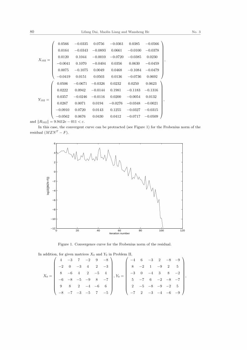
80 Lifang Dai, Maolin Liang and Wansheng He No. 3
X102 =
0.0566 −0.0335 0.0756 −0.0361 0.0385 −0.0566
0.0164 −0.0343 −0.0893 0.0661 −0.0100 −0.0378
0.0120 0.1044 −0.0010 −0.0720 −0.0385 0.0230
−0.0041 0.1070 −0.0404 0.0356 0.0630 −0.0459
0.0075 −0.1075 0.0049 0.0468 −0.1084 −0.0479
−0.0419 0.0151 0.0503 0.0136 −0.0736 0.0692
,
Y102 =
0.0506 −0.0671 −0.0326 0.0232 0.0250 0.0623
0.0222 0.0942 −0.0144 0.1981 −0.1183 −0.1316
0.0357 −0.0246 −0.0116 0.0200 −0.0054 0.0132
0.0267 0.0071 0.0194 −0.0276 −0.0348 −0.0021
−0.0910 0.0720 0.0143 0.1255 −0.0327 −0.0315
−0.0562 0.0676 0.0430 0.0412 −0.0717 −0.0509
,
and ‖R102‖ = 9.9412e− 011 < ε.
In this case, the convergent curve can be protracted (see Figure 1) for the Frobenius norm of the
residual (MZNT − F ).
0 20 40 60 80 100 120−12
−10
−8
−6
−4
−2
0
2
4
6
iteration number
log1
0(||M
ZN−F
||)
Figure 1. Convergence curve for the Frobenius norm of the residual.
In addition, for given matrices X0 and Y0 in Problem II,
X0 =
4 −3 7 −2 9 −8
−2 0 −3 4 2 −3
8 −6 4 2 −5 4
−6 −8 −5 −9 8 −7
9 8 2 −4 −6 6
−8 −7 −3 −5 7 −5
, Y0 =
−4 6 −3 2 −8 −9
8 −2 1 −9 2 5
−3 0 −4 3 8 −2
5 −7 6 −2 −8 −7
2 −5 −8 −9 −2 5
−7 2 −3 −4 −6 −9
,

Vol. 6 Iterative method for the solution of linear matrix equation AXBT + CY DT = F 81
let Z0 = UT
X0 0
0 Y0
U , Writing Z = Z −Z0, and F = F −MZ0N
T . Applying Algorithm 2.1 to
matrix equation (11), we obtain its least-norm solution
Z∗ =
−5.8153 −0.2782 4.7702 0 −0.8438 −3.6153
2.3393 2.7852 2.7168 0 2.0293 3.8334
2.0181 1.5966 −4.6136 0 −7.8829 −3.3454
0 0 0 0.8932 0 0
3.5404 2.8399 −2.4268 0 0.9133 −3.6829
2.5268 2.1881 −1.1341 0 −2.4191 4.6972
0 0 0 1.3810 0 0
0 0 0 5.5758 0 0
−3.4825 −2.8830 0.0799 0 1.3228 −0.2273
0 0 0 −2.0380 0 0
0 0 0 −1.2799 0 0
0 0 0 3.0779 0 0
0 0 −5.9629 0 0 0
0 0 2.0185 0 0 0
0 0 −0.7883 0 0 0
1.3495 −1.5618 0 −1.8001 1.5674 −1.8388
0 0 −1.7462 0 0 0
0 0 −1.3801 0 0 0
−0.6582 0.6536 0 −3.1742 0.3432 −1.2151
−4.3037 −0.9233 0 −1.1176 6.6026 7.3582
0 0 −0.7266 0 0 0
3.6177 2.1986 0 −4.7265 −0.3212 −6.2395
−1.9036 1.5179 0 4.1862 −3.2106 4.2403
0.6987 −1.9882 0 −4.0467 3.9708 −1.6224
,
Hence, it follows from equality (12) that the unique optimal solution pair (X, Y ) of Problem II
can be expressed as
X =
−1.8153 −3.8438 2.2298 −1.7218 3.0371 −4.3847
1.5404 0.9133 −0.5732 1.1601 0.2538 0.6829
5.9819 1.8829 −0.6136 3.5966 −4.2117 0.6546
−8.3393 −10.0293 −2.2832 −6.2148 5.9815 −3.1666
5.5175 9.3228 1.9201 −1.1170 −6.7266 6.2273
−10.5268 −4.5809 −4.1341 −2.8119 8.3801 −0.3028
,

82 Lifang Dai, Maolin Liang and Wansheng He No. 3
Y =
−4.6582 5.3464 −1.6190 0.7849 −11.1742 −9.3432
12.3037 −2.9233 −4.5758 −16.3582 3.1176 11.6026
−1.6505 1.5618 −3.1068 1.1612 6.1999 −3.5674
5.6987 −5.0118 9.0779 −3.6224 −12.0467 −10.9708
5.6177 −7.1986 −10.0380 −15.2395 −6.7265 5.3212
−5.0964 3.5179 −1.7201 −8.2403 −10.1862 −12.2106
.
Example 4.2. Let M and N be a 100 × 100 matrix with element Mij = − 1(i+j+1)
, (i, j =
1, 2, ..., 100) and a 100 × 100 tri-diagonal matrix with diagonal elements equal to 4 and off-diagonal
elements equal to (−1,− 12, ...,− 1
99) and (1, 1
2, ..., 1
99), respectively, and P be a matrix with second-
diagonal elements equal to 1 and all other elements equal to 0. Let F = MZNT , where Z be 100×100
matrix with all elements 1. Then the matrix equation (3) is consistent since the above matrix Z is
one of its solutions. Using Algorithm 2.1 and iterating 350 (¿ 10000) steps, we paint the convergence
curve in Figure 2 for the Frobenius norm of the residual (MZNT − F ).
0 50 100 150 200 250 300 350−14
−12
−10
−8
−6
−4
−2
0
2
4
6
iteration number
log1
0(||M
ZN−F
||)
Figure 2. Convergence curve for the Frobenius norm of the residual.
From the convergency curve in Figure 2, we can see that the iterative algorithm in this paper is
efficient.
The following example subjects to the conclusion in Corollary 1.
Example 4.3. Input matrices B, D, F, U, P as in Example 4.1, let A = C = ones(6), and denote
M = (A, C)U, N = (B, D)U .
Making use of Algorithm 2.1 solves Problem I. Let initial iterative matrix Z1 = 0 ∈ R6×6, we get
from the 7th iteration that
‖R7‖ = 5.0321e + 003 À ‖P7‖ = 2.9759.
From Corollary I, we know that matrix equation (1) is inconsistent.

Vol. 6 Iterative method for the solution of linear matrix equation AXBT + CY DT = F 83
References
[1] J. K. Baksalary, R. Kala, The matrix equation AX − Y B = C, Linear Algebra Appl., 25
(1979), 41-43.
[2] H. Flanders, H.K. Wimmer, On the matrix equation AX−XB = C and AX−Y B = C, SIAM
J. Appl. Math, 32(1977), 707-710.
[3] J. K. Baksalary, R. Kala, The matrix equation AXB + CY D = E, Linear Algebra Appl, 30
(1980), 141-147.
[4] K. E. Chu, Singular value and generalized singular value decompositions and the solution of
linear matrix equations, Linear Algebra Appl, 88/89(1987), 83-98.
[5] C. N. He, The general Solution of the matrix equation AXB + CY D = F , Acta Sei Nat Univ
Norm Hunan, China, 19(1996), 17-20.
[6] G. P. Xu, M. S. Wei, D.-S. Zheng, On solutions of matrix equation AXB + CY D = F , Linear
Algebra Appl, 279(1998), 93-109.
[7] X. W. Chang. J. S. Wang, The symmetric solution of the matrix equations AX + Y A = C,
AXAT + BY BT = C and (AT XA, BT XB) = (C, D), Linear Algebra Appl., 179 (1993), 171-189.
[8] Y. X. Peng, An iterative method for the symmetric solutions and the optimal approximation
solution of the linear matrix equation AXB = C, Appl. Math. Comput., 160 (2005), 763-777.
[9] Z. Y. Peng, An iterative method for the least-squares symmetric solution of the linear matrix
equation AXB = C, Appl. Math. Comput, 170(2005), 711-723.
[10] Y. X. Peng, X. Y. Hu and L. Zhang, An iterative method for symmetric solutions and optimal
approximation solution of the system of matrix equations A1XB1 = C1, A2XB2 = C2, Appl. Math.
Comput, 183(2006), No. 2, 1127-1137.
[11] M. H. Wang, X. H. Cheng, M. S. Wei, Iterative algorithms for solving the matrix equation
AXB + CXT D = E, Appl. Math. Comput, 187(2007), No. 2, 622-629.
[12] Z. Y. Peng, Y. X. Peng, An efficient iterative method for solving the matrix equation AXB +
CY D = E, Numer. Linear Algebra Appl, 13(2006), 473-485.
[13] T. Meng, Experimental design and decision support, in: Leondes (Ed.), Expert Systems, the
Technology of Knowledgy Managenment and Decision Making for the 21th Century, Vol. 1, Academic
Press, 2001.
[14] A. P. Liao, Z. Z. Bai, Best approximation of matrix equation AXB + CY D = E, SIAM J.
Matrix Anal. Appl, 27(2005), 675-688.
[15] M. L. Liang, C. H. You, L. F. Dai, An efficient algorithm for the generalized centro-symmetric
solution of matrix equation AXB = C, Numer. Algor, 44(2007), 173-184.
[16] J. L. Chen, X. H. Chen, Special Matrix, Tsinghua Univ. Press (in Chinese), 2001.
[17] Z. Xu, K. Y. Zhang, Q. Lu, A fast algorithm for a class of Toeplitz matrix (in Chinese), Xibei
Univ. Industry Press, 1999.
[18] Weaver J. R., Centrosymmetric matrices, their basic properties, eigenvalues, and eigenvectors,
Amer. Math. Monthly, 92 (1985), 711-717.

Scientia MagnaVol. 6 (2010), No. 3, 84-88
Smarandachely antipodal signed digraphs
P. Siva Kota Reddy†, B. Prashanth† and M. Ruby Salestina‡
† Department of Mathematics Acharya Institute of Technology,Bangalore 560090, India
‡ Department of Mathematics Yuvaraja’s College, University of Mysore,Mysore 570005, India
E-mail: [email protected] [email protected]@rediffmail.com
Abstract A Smarandachely k-signed digraph (Smarandachely k-marked digraph) is an or-
dered pair S = (D, σ) (S = (D, µ)) where D = (V,A) is a digraph called underlying digraph
of S and σ : A → (e1, e2, ..., ek) (µ : V → (e1, e2, ..., ek)) is a function, where each ei ∈ +,−.Particularly, a Smarandachely 2-signed digraph or Smarandachely 2-marked digraph is called
abbreviated a signed digraph or a marked digraph. In this paper, we define the Smarandachely
antipodal signed digraph−→A (D) of a given signed digraph S = (D, σ) and offer a structural
characterization of antipodal signed digraphs. Further, we characterize signed digraphs S for
which S ∼ −→A (S) and S ∼ −→
A (S) where ∼ denotes switching equivalence and−→A (S) and S are
denotes the Smarandachely antipodal signed digraph and complementary signed digraph of S
respectively.
Keywords Smarandachely k-signed digraphs, Smarandachely k-marked digraphs, balance,
switching, Smarandachely antipodal signed digraphs, negation.
§1. Introduction
For standard terminology and notion in digraph theory, we refer the reader to the classictext-books of Bondy and Murty [1] and Harary et al.[3]; the non-standard will be given in thispaper as and when required.
A Smarandachely k-signed digraph (Smarandachely k-marked digraph) is an ordered pairS = (D, σ) (S = (D, µ)) where D = (V,A) is a digraph called underlying digraph of S and σ :A → (e1, e2, ..., ek) (µ : V → (e1, e2, ..., ek)) is a function, where each ei ∈ +,−. Particularly,a Smarandachely 2-signed digraph or Smarandachely 2-marked digraph is called abbreviateda signed digraph or a marked digraph. A signed digraph is an ordered pair S = (D, σ), whereD = (V,A) is a digraph called underlying digraph of S and σ : A → +,− is a function.A marking of S is a function µ : V (D) → +,−. A signed digraph S together with amarking µ is denoted by Sµ. A signed digraph S = (D, σ) is balanced if every semicycle of S
is positive (Harary et al.[3]). Equivalently, a signed digraph is balanced if every semicycle hasan even number of negative arcs. The following characterization of balanced signed digraphs isobtained by E. Sampathkumar et al.[5].

Vol. 6 Smarandachely antipodal signed digraphs 85
Proposition 1.1.[5] A signed digraph S = (D, σ) is balanced if, and only if, there exist amarking µ of its vertices such that each arc −→uv in S satisfies σ(−→uv) = µ(u)µ(v).
Let S = (D, σ) be a signed digraph. Consider the marking µ on vertices of S definedas follows: each vertex v ∈ V , µ(v) is the product of the signs on the arcs incident at v.Complement of S is a signed digraph S = (D, σ′), where for any arc e = −→uv ∈ D, σ′(−→uv) =µ(u)µ(v). Clearly, S as defined here is a balanced signed digraph due to Proposition 1.1.
In [5], the authors define switching and cycle isomorphism of a signed digraph as follows:Let S = (D, σ) and S′ = (D′, σ′), be two signed digraphs. Then S and S′ are said to be
isomorphic, if there exists an isomorphism φ : D → D′ (that is a bijection φ : V (D) → V (D′)such that if −→uv is an arc in D then
−−−−−−→φ(u)φ(v) is an arc in D′) such that for any arc −→e ∈ D,
σ(−→e ) = σ′(φ(−→e )). For switching in signed graphs and some results involving switching referthe paper [4].
Given a marking µ of a signed digraph S = (D, σ), switching S with respect to µ isthe operation changing the sign of every arc −→uv of S′ by µ(u)σ(−→uv)µ(v). The signed digraphobtained in this way is denoted by Sµ(S) and is called µ switched signed digraph or just switchedsigned digraph.
Further, a signed digraph S switches to signed digraph S′ (or that they are switchingequivalent to each other), written as S ∼ S′, whenever there exists a marking of S such thatSµ(S) ∼= S′.
Two signed digraphs S = (D, σ) and S′ = (D′, σ′) are said to be cycle isomorphic, if thereexists an isomorphism φ : D → D′ such that the sign σ(Z) of every semicycle Z in S equals tothe sign σ(φ(Z)) in S′.
Proposition 1.2.[4] Two signed digraphs S1 and S2 with the same underlying graph areswitching equivalent if, and only if, they are cycle isomorphic.
§2. Smarandachely antipodal signed digraphs
In [2], the authors introduced the notion antipodal digraph of a digraph as follows: For adigraph D = (V,A), the antipodal digraph
−→A (D) of D = (V,A) is the digraph with V (
−→A (D)) =
V (D) and A(−→A (D)) = (u, v) : u, v ∈ V (D) and dD(u, v) = diam(D).
We extend the notion of−→A (D) to the realm of signed digraphs. In a signed digraph
S = (D, σ), where D = (V,A) is a digraph called underlying digraph of S and σ : A → +,− isa function. The Smarandachely antipodal signed digraph
−→A (S) = (
−→A (D), σ′) of a signed digraph
S = (D, σ) is a signed digraph whose underlying digraph is−→A (D) called antipodal digraph and
sign of any arc e = −→uv in−→A (S), σ′(e) = µ(u)µ(v), where for any v ∈ V , µ(v) =
∏
u∈N(v)
σ(uv).
Further, a signed digraph S = (D, σ) is called Smarandachely antipodal signed digraph, ifS ∼= −→
A (S′), for some signed digraph S′. The following result indicates the limitations ofthe notion
−→A (S) as introduced above, since the entire class of unbalanced signed digraphs is
forbidden to be antipodal signed digraphs.Proposition 2.1. For any signed digraph S = (D, σ), its Smarandachely antipodal signed
graph A(S) is balanced.

86 P. Siva Kota Reddy, B. Prashanth and M. Ruby Salestina No. 3
Proof. Since sign of any arc e = −→uv in−→A (S) is µ(u)µ(v), where µ is the canonical marking
of S, by Proposition 1.1,−→A (S) is balanced.
For any positive integer k, the kth iterated antipodal signed digraph−→A (S) of S is defined
as follows:−→A 0(S) = S, Ak(S) =
−→A (−→Ak−1(S)).
Corollary 2.2. For any signed digraph S = (D, σ) and any positive integer k,−→Ak(S) is
balanced.In [2], the authors characterized those digraphs that are isomorphic to their antipodal
digraphs.Proposition 2.3.[2] For a digraph D = (V,A), D ∼= −→
A (D) if, and only if, D ∼= K∗p .
Proof. First, suppose that D ∼= −→A (D). If (u, v) ∈ A then (u, v) ∈ A(
−→A (D)). Therefore,
dD(u, v) = 1 = diam(D). Since K∗p is the only digraph of diameter 1, we have D ∼= K∗
p .For the converse, if D ∼= K∗
p , then diam(D) = 1 and for every pair u, v of vertices in D,the distance dD(u, v) = 1. Hence,
−→A (D) ∼= K∗
p and D ∼= −→A (D).
We now characterize the signed digraphs that are switching equivalent to their Smaran-dachely antipodal signed graphs.
Proposition 2.4. For any signed digraph S = (D, σ), S ∼ −→A (S) if, and only if, D ∼= K∗
p
and S is balanced signed digraph.Proof. Suppose S ∼ −→
A (S). This implies, D ∼= −→A (D) and hence D is K∗
p . Now, if S is anysigned digraph with underlying digraph as K∗
p , Proposition 2.1 implies that−→A (S) is balanced
and hence if S is unbalanced and its−→A (S) being balanced can not be switching equivalent to
S in accordance with Proposition 1.2. Therefore, S must be balanced.Conversely, suppose that S is an balanced signed digraph and D is K∗
p . Then, since−→A (S)
is balanced as per Proposition 2.1 and since D ∼= −→A (D), the result follows from Proposition 1.2
again.Proposition 2.5. For any two signed digraphs S and S′ with the same underlying digraph,
their Smarandachely antipodal signed digraphs are switching equivalent.Proposition 2.6.[2] For a digraph D = (V,A), D ∼= −→
A (D) if, and only if,i) diam(D) = 2.ii) D is not strongly connected and for every pair u, v of vertices of D, the distance
dD(u, v) = 1 or dD(u, v) = ∞.In view of the above, we have the following result for signed digraphs:Proposition 2.7. For any signed digraph S = (D, σ), S ∼ −→
A (S) if, and only if, D satisfiesconditions of Proposition 2.6.
Proof. Suppose that−→A (S) ∼ S. Then clearly we have
−→A (D) ∼= D and hence D satisfies
conditions of Proposition 2.6.Conversely, suppose that D satisfies conditions of Proposition 2.6. Then D ∼= −→
A (D) byProposition 2.6. Now, if S is a signed digraph with underlying digraph satisfies conditions ofProposition 2.6, by definition of complementary signed digraph and Proposition 2.1, S and−→A (S) are balanced and hence, the result follows from Proposition 1.2.
The notion of negation η(S) of a given signed digraph S defined in [6] as follows: η(S) hasthe same underlying digraph as that of S with the sign of each arc opposite to that given to it

Vol. 6 Smarandachely antipodal signed digraphs 87
in S. However, this definition does not say anything about what to do with nonadjacent pairsof vertices in S while applying the unary operator η(.) of taking the negation of S.
Proposition 2.4 & 2.7 provides easy solutions to two other signed digraph switching equiv-alence relations, which are given in the following results.
Corollary 2.8. For any signed digraph S = (D, σ), S ∼ −→A (η(S)).
Corollary 2.9. For any signed digraph S = (D, σ), S ∼ −→A (η(S)).
Problem. Characterize signed digraphs for which
i) η(S) ∼ −→A (S).
ii) η(S) ∼ −→A (S).
For a signed digraph S = (D, σ), the−→A (S) is balanced (Proposition 2.1). We now examine,
the conditions under which negation η(S) of−→A (S) is balanced.
Proposition 2.10. Let S = (D, σ) be a signed digraph. If−→A (G) is bipartite then η(
−→A (S))
is balanced.
Proof. Since, by Proposition 2.1,−→A (S) is balanced, if each semicycle C in
−→A (S) contains
even number of negative arcs. Also, since−→A (D) is bipartite, all semicycles have even length;
thus, the number of positive arcs on any semicycle C in−→A (S) is also even. Hence η(
−→A (S)) is
balanced.
§3. Characterization of Smarandachely antipodal signed
graphs
The following result characterize signed digraphs which are Smarandachely antipodal signeddigraphs.
Proposition 3.1. A signed digraph S = (D, σ) is a Smarandachely antipodal signeddigraph if, and only if, S is balanced signed digraph and its underlying digraph D is an antipodalgraph.
Proof. Suppose that S is balanced and D is a−→A (D). Then there exists a digraph H such
that−→A (H) ∼= D. Since S is balanced, by Proposition 1.1, there exists a marking µ of D such
that each arc −→uv in S satisfies σ(−→uv) = µ(u)µ(v). Now consider the signed digraph S′ = (H, σ′),where for any arc e in H, σ′(e) is the marking of the corresponding vertex in D. Then clearly,−→A (S′) ∼= S. Hence S is an Smarandachely antipodal signed digraph.
Conversely, suppose that S = (D, σ) is a Smarandachely antipodal signed digraph. Thenthere exists a signed digraph S′ = (H, σ′) such that
−→A (S′) ∼= S. Hence D is the A(D) of H
and by Proposition 2.1, S is balanced.
Acknowledgement
The first two authors would like to acknowledge and extend their heartfelt gratitude to Sri.B. Premnath Reddy, Chairman, Acharya Institutes, for his vital encouragement and support.

88 P. Siva Kota Reddy, B. Prashanth and M. Ruby Salestina No. 3
References
[1] J. A. Bondy and U. S. R. Murty, Graph Theory with Applications, MacMillan, London,1976.
[2] G. Johns and K. Sleno, Antipodal graphs and digraphs, Internat. J. Math. & Math.Sci., 16(1993), No. 3, 579-586.
[3] F. Harary, R. Norman and D. Cartwright, Structural models: An introduction to thetheory of directed graphs, J. Wiley, New York, 1965.
[4] R. Rangarajan and P. Siva Kota Reddy, The edge C4 signed graph of a signed graph,Southeast Asian Bull. Math., 34(2010), No. 6, 1077-1082.
[5] E. Sampathkumar, M. S. Subramanya and P. Siva Kota Reddy, Characterization ofLine Sidigraphs, Southeast Asian Bull. Math., to appear.
[6] P. Siva Kota Reddy, S. Vijay and H. C. Savithri, A Note on Path Sidigraphs, Interna-tional J. Math. Combin., 1(2010), 42-46.

Scientia MagnaVol. 6 (2010), No. 3, 89-92
Smarandachely t-path step signed graphs
P. Siva Kota Reddy†, B. Prashanth‡ and V. Lokesha]
Department of Mathematics, Acharya Institute of Technology,Bangalore-560 090, India
E-mail: [email protected] [email protected] [email protected]
Abstract A Smarandachely k-signed graph (Smarandachely k-marked graph) is an ordered
pair S = (G, σ) (S = (G, µ)) where G = (V, E) is a graph called underlying graph of S and
σ : E → (e1, e2, · · · , ek) (µ : V → (e1, e2, · · · , ek)) is a function, where each ei ∈ +,−.Particularly, a Smarandachely 2-signed graph or Smarandachely 2-marked graph is called
abbreviated a signed graph or a marked graph. E. Prisner [9] in his book Graph Dynamics
defines the t-path step operator on the class of finite graphs. Given a graph G and a positive
integer t, the t-path step graph (G)t of G is formed by taking a copy of the vertex set V (G)
of G, joining two vertices u and v in the copy by a single edge e = uv whenever there exists a
u− v path of length t in G. Analogously, one can define the Smarandachely t-path step signed
graph (S)t = ((G)t, σ′) of a signed graph S = (G, σ) is a signed graph whose underlying graph
is (G)t called t-path step graph and sign of any edge e = uv in (S)t is µ(u)µ(v). It is shown
that for any signed graph S, its (S)t is balanced. We then give structural characterization
of Smarandachely t-path step signed graphs. Further, in this paper we characterize signed
graphs which are switching equivalent to their Smarandachely 3-path step signed graphs.
Keywords Smarandachely k-signed graphs, Smarandachely k-marked graphs, signed graphs,
marked graphs, balance, switching, Smarandachely t-path step signed graphs, negation.
§1. Introduction
For standard terminology and notion in graph theory we refer the reader to Harary [4];the non-standard will be given in this paper as and when required. We treat only finite simplegraphs without self loops and isolates.
A Smarandachely k-signed graph (Smarandachely k-marked graph) is an ordered pair S =(G, σ) (S = (G,µ)) where G = (V, E) is a graph called underlying graph of S and σ : E →(e1, e2, · · · , ek) (µ : V → (e1, e2, · · · , ek)) is a function, where each ei ∈ +,−. Particularly, aSmarandachely 2-signed graph or Smarandachely 2-marked graph is called abbreviated a signedgraph or a marked graph. A signed graph S = (G, σ) is balanced if every cycle in S has an evennumber of negative edges (Harary [3]). Equivalently a signed graph is balanced if product ofsigns of the edges on every cycle of S is positive.
A marking of S is a function µ : V (G) → +,−; A signed graph S together with amarking µ by Sµ. Given a signed graph S one can easily define a marking µ of S as follows:

90 P. Siva Kota Reddy, B. Prashanth and V. Lokesha No. 3
For any vertex v ∈ V (S),
µ(v) =∏
u∈N(v)
σ(uv),
the marking µ of S is called canonical marking of S.The following characterization of balanced signed graphs is well known.Proposition 1.1.[6] A signed graph S = (G, σ) is balanced if, and only if, there exist a
marking µ of its vertices such that each edge uv in S satisfies σ(uv) = µ(u)µ(v).Given a marking µ of S, by switching S with respect to µ we mean reversing the sign of
every edge of S whenever the end vertices have opposite signs in Sµ[1] . We denote the signed
graph obtained in this way is denoted by Sµ(S) and this signed graph is called the µ-switchedsigned graph or just switched signed graph. A signed graph S1 switches to a signed graph S2
(that is, they are switching equivalent to each other), written S1 ∼ S2, whenever there exists amarking µ such that Sµ(S1) ∼= S2.
Two signed graphs S1 = (G, σ) and S2 = (G′, σ′) are said to be weakly isomorphic(Sozansky [7] ) or cycle isomorphic (Zaslavsky [8]) if there exists an isomorphism φ : G → G′
such that the sign of every cycle Z in S1 equals to the sign of φ(Z) in S2. The following resultis well known:
Proposition 1.2.[8] Two signed graphs S1 and S2 with the same underlying graph areswitching equivalent if, and only if, they are cycle isomorphic.
§2. Smarandachely t-path step signed graphs
Given a graph G and a positive integer t, the t-path step graph (G)t of G is formed bytaking a copy of the vertex set V (G) of G, joining two vertices u and v in the copy by a singleedge e = uv whenever there exists a u − v path of length t in G. The notion of t-path stepgraphs was defined in [9], page 168.
In this paper, we shall now introduce the concept of Smarandachely t-path step signedgraphs as follows: The Smarandachely t-path step signed graph (S)t = ((G)t, σ
′) of a signedgraph S = (G, σ) is a signed graph whose underlying graph is (G)t called t-path step graph andsign of any edge e = uv in (S)t is µ(u)µ(v), where µ is the canonical marking of S. Further,a signed graph S = (G, σ) is called Smarandachely t-path step signed graph, if S ∼= (S′)t, forsome signed graph S′.
The following result indicates the limitations of the notion of Smarandachely t-path stepsigned graphs as introduced above, since the entire class of unbalanced signed graphs is forbiddento be Smarandachely t-path step signed graphs.
Proposition 2.1. For any signed graph S = (G, σ), its (S)t is balanced.Proof. Since sign of any edge e = uv is (S)t is µ(u)µ(v), where µ is the canonical marking
of S, by Proposition 1.1, (S)t is balanced.Remark. For any two signed graphs S and S′ with same underlying graph, their Smaran-
dachely t-path step signed graphs are switching equivalent.Corollary 2.2. For any signed graph S = (G, σ), its Smarandachely 2 (3)-path step signed
graph (S)2 ((S)3) is balanced.

Vol. 6 Smarandachely t-path step signed graphs 91
The following result characterize signed graphs which are Smarandachely t-path step signedgraphs.
Proposition 2.3. A signed graph S = (G, σ) is a Smarandachely t-path step signed graphif, and only if, S is balanced signed graph and its underlying graph G is a t-path step graph.
Proof. Suppose that S is balanced and G is a t-path step graph. Then there exists agraph H such that (H)t
∼= G. Since S is balanced, by Proposition 1.1, there exists a markingµ of G such that each edge e = uv in S satisfies σ(uv) = µ(u)µ(v). Now consider the signedgraph S′ = (H, σ′), where for any edge e in H, σ′(e) is the marking of the corresponding vertexin G. Then clearly, (S′)t
∼= S. Hence S is a Smarandachely t-path step signed graph.Conversely, suppose that S = (G, σ) is a Smarandachely t-path step signed graph. Then
there exists a signed graph S′ = (H, σ′) such that (S′)t∼= S. Hence G is the t-path step graph
of H and by Proposition 2.1, S is balanced.
§3. Switching invariant Smarandachely 3-path step signed
graphs
Zelinka [9] prove hat the graphs in Fig. 1 are all unicyclic graphs which are fixed in theoperator (G)3, i.e. graphs G such that G ∼= (G)3. The symbols p, q signify that the number ofvertices and edges in Fig. 1.
Proposition 3.1.[9] Let G be a finite unicyclic graph such that G ∼= (G)3. Then either G
is a circuit of length not divisible by 3, or it is some of the graphs depicted in Fig. 1.
cc c
cc c
c
c
c
s
c c
c c
c cc
c
cccc
cccc
p >= 0, q >= 0
p q
Fig.1.
In view of the above result, we have the following result for signed graphs:Proposition 3.2. For any signed graph S = (G, σ), S ∼ (S)3 if, and only if, G is a cycle
of length not divisible by 3, or it is some of the graphs depicted in Fig. 1 and S is balanced.Proof. Suppose S ∼ (S)3. This implies, G ∼= (G)3 and hence by Proposition 3.1, we see
that the G must be isomorphic to either Cm, 4 ≤ m 6= 3k, k is a positive integer or the graphsdepicted in Fig. 1. Now, if S is any signed graph on any of these graphs, Corollary 4 impliesthat (S)3 is balanced and hence if S is unbalanced its Smarandachely 3-path step signed graph(S)3 being balanced cannot be switching equivalent to S in accordance with Proposition 1.2.Therefore, S must be balanced.

92 P. Siva Kota Reddy, B. Prashanth and V. Lokesha No. 3
Conversely, suppose that S is a balanced signed graph on Cm, 4 ≤ m 6= 3k, k is a positiveinteger or the graphs depicted in Fig. 1. Then, since (S)3 is balanced as per Corollary 2.2 andsince G ∼= (G)3 in each of these cases, the result follows from Proposition 1.2.
Problem. Characterize the signed graphs for which S ∼= (S)3.The notion of negation η(S) of a given signed graph S defined by Harary [3] as follows: η(S)
has the same underlying graph as that of S with the sign of each edge opposite to that givento it in S. However, this definition does not say anything about what to do with nonadjacentpairs of vertices in S while applying the unary operator η(.) of taking the negation of S.
For a signed graph S = (G, σ), the (S)t is balanced (Proposition 2.1). We now examine,the condition under which negation of (S)t (i.e., η((S)t)) is balanced.
Proposition 3.3. Let S = (G, σ) be a signed graph. If (G)t is bipartite then η((S)t) isbalanced.
Proof. Since, by Proposition 2.1, (S)t is balanced, then every cycle in (S)t contains evennumber of negative edges. Also, since (G)t is bipartite, all cycles have even length; thus, thenumber of positive edges on any cycle C in (S)t are also even. This implies that the same thingis true in negation of (S)t. Hence η((S)t) is balanced.
Proposition 3.2 provides easy solutions to three other signed graph switching equivalencerelations, which are given in the following results.
Corollary 3.4. For any signed graph S = (G, σ), η(S) ∼ (S)3 if, and only if, S isunbalanced signed graph on C2m+1, m ≥ 2 or first two graphs depicted in Fig. 1.
Corollary 3.5. For any signed graph S = (G, σ), (η(S))3 ∼ (S)3.
References
[1] R. P. Abelson and M. J. Rosenberg, Symoblic psychologic, A model of attitudinalcognition, Behav. Sci., 3(1958), 1-13.
[2] F. Harary, On the notion of balance of a sigraph, Michigan Math. J., 2 (1953), 143-146.[3] F. Harary, Structural duality, Behav. Sci., 2(1957), No. 4, 255-265.[4] F. Harary, Graph Theory, Addison-Wesley Publishing Co., 1969.[5] E. Prisner, Graph Dynamics, Longman House, Burnt Mill, Harlow, 1998.[6] E. Sampathkumar, Point signed and line signed graphs, Nat. Acad. Sci. Letters,
7(1984), No. 3, 91-93.[7] T. Sozansky, Enueration of weak isomorphism classes of signed graphs, J. Graph Theory,
4(1980), No. 2, 127-144.[8] T. Zaslavsky, Signed Graphs, Discrete Appl. Math., 4(1982), No. 1, 47-74.[9] B. Zelinka, The 3-path-step operator on trees and unicyclic graphs, Mathematica Bo-
hemica, 127(2002), No. 1, 33-40.

Scientia MagnaVol. 6 (2010), No. 3, 93-98
On a note of the Smarandache power function 1
Wei Huang† and Jiaolian Zhao‡
† Department of Basis, Baoji Vocational and Technical College,Baoji 721013, China
‡ Department of Mathematics, Weinan Teacher’s University,Weinan 714000, China
E-mail: [email protected]
Abstract For any positive integer n, the Smarandache power function SP (n) is defined as the
smallest positive integer m such that n|mm, where m and n have the same prime divisors. The
main purpose of this paper is to study the distribution properties of the k−th power of SP (n)
by analytic methods, obtain three asymptotic formulas of∑
n≤x
(SP (n))k,∑
n≤x
ϕ((SP (n))k) and
∑n≤x
d(SP (n))k (k > 1), and supplement the relate conclusions in some references.
Keywords Smarandache power function, the k − th power, mean value, asymptotic formula.
§1. Introduction and results
For any positive integer n, we define the Smarandache power function SP (n) as the smallestpositive integer m such that n|mm, where n and m have the same prime divisors. That is,
SP (n) = min
m : n|mm,m ∈ N+,∏
p|mp =
∏
p|np
.
If n runs through all natural numbers, then we can get the Smarandache power function se-quence SP (n): 1, 2, 3, 2, 5, 6, 7, 4, 3, 10, 11, 6, 13, 14, 15, 4, 17, 6, 19, 10, · · · , Let n = pα1
1 pα22 · · · pαk
k ,denotes the factorization of n into prime powers. If αi < pi, for all αi (i = 1, 2, · · · , r), thenwe have SP (n) = U(n), where U(n) =
∏p|n
p,∏p|n
denotes the product over all different prime
divisors of n. It is clear that SP (n) is not a multiplicative function.In reference [1], Professor F. Smarandache asked us to study the properties of the sequence
SP (n). He has done the preliminary research about this question literature [2] − [4], hasobtained some important conclusions. And literature [2] has studied an average value, obtainedthe asymptotic formula:
∑
n≤x
SP (n) =12x2
∏p
(1− 1
p(1 + p)
)+ O
(x
32+ε
).
1This paper was partially supported by National Natural Science Foundation of China (10671155), The
Natural Sciences Funding of Project Shaanxi Province (SJ08A28) and The Educational Sciences Funding Project
of Shaanxi Province (2010JK541).
94 Wei Huang and Jiaolian Zhao No. 3
Literature [3] has studied the infinite sequence astringency, has given the identical equation:
∞∑n=1
(−1)µ(n)
(SP (nk))s=
2s + 1(2s − 1)ζ(s)
, k = 1, 2;
2s + 1(2s − 1)ζ(s)
− 2s − 14s
, k = 3;
2s + 1(2s − 1)ζ(s)
− 2s − 14s
+3s − 1
9s, k = 4, 5.
And literature [4] has studied the equation SP (nk) = φ(n), k = 1, 2, 3 solubility (φ(n) is theEuler function), and has given all positive integer solution. Namely the equation SP (n) = φ(n)only has 4 positive integer solutions n = 1, 4, 8, 18; Equation SP (n3) = φ(n) to have andonly has 3 positive integer solutions n = 1, 16, 18. In this paper, we shall use the analysismethod to study the distribution properties of the k − th power of SP (n), gave
∑n≤x
(SP (n))k,∑
n≤x
ϕ((SP (n))k) and∑
n≤x
d(SP (n))k (k > 1), some interesting asymptotic formula, has pro-
moted the literature [2] conclusion.Specifically as follows:Theorem 1.1. For any random real number x ≥ 3 and given real number k (k > 0), we
have the asymptotic formula:
∑
n≤x
(SP (n))k =ζ(k + 1)
(k + 1)ζ(2)xk+1
∏p
(1− 1
pk(p + 1)
)+ O(xk+ 1
2+ε);
∑
n≤x
(SP (n))k
n=
ζ(k + 1)kζ(2)
xk∏p
(1− 1
pk(p + 1)
)+ O(xk+ 1
2+ε),
where ζ(k) is the Riemann zeta-function, ε denotes any fixed positive number, and∏p
denotes
the product over all primes.Corollary 1.1. For any random real number x ≥ 3 and given real number k′ > 0 we have
the asymptotic formula:
∑
n≤x
(SP (n))1k′ =
6k′ζ( 1+k′k′ )
(k′ + 1)π2x
1+k′k′
∏p
(1− 1
(1 + p)p1k′
)+ O
(x
k′+22k′ +ε
).
Specifically, we have
∑
n≤x
(SP (n))12 =
4ζ( 32 )
π2x
32
∏p
(1− 1
(1 + p)p12
)+ O(x1+ε);
∑
n≤x
(SP (n))13 =
9ζ( 43 )
2π2x
43
∏p
(1− 1
(1 + p)p13
)+ O(x
56+ε).
Corollary 1.2. For any random real number x ≥ 3, and k = 1, 2, 3. We have the asymp-totic formula: ∑
n≤x
(SP (n)) =12x2
∏p
(1− 1
p(1 + p)
)+ O(x
32+ε);
∑
n≤x
(SP (n))2 =6ζ(3)3π2
x3∏p
(1− 1
p2(1 + p)
)+ O(x
52+ε);
Vol. 6 On a note of the Smarandache power function 95
∑
n≤x
(SP (n))3 =π2
60x4
∏p
(1− 1
p3(1 + p)
)+ O(x
72+ε).
Theorem 1.2. For any random real number x ≥ 3, we have the asymptotic formula:
∑
n≤x
ϕ((SP (n))k
)=
ζ(k + 1)(k + 1)ζ(2)
xk+1∏p
(1− 1
(1 + p)pk
)+ O(xk+ 1
2+ε),
where ϕ(n) is the Euler functionTheorem 1.3. For any random real number x ≥ 3, we have the asymptotic formula:
∑
n≤x
d((SP (n))k
)= B0x lnk x + B1x lnk−1 x + B2x lnk−2 x + · · ·+ Bk−1x lnx + Bkx + O(x
12+ε).
where d(n) is the Dirichlet divisor function and B0, B1, B2, · · · , Bk−1, Bk is computable con-stant.
§2. Lemmas and proofs
Suppose s = σ + it and let n = pα11 pα2
2 · · · pαk
k , U(n) =∏p|n
p. Before the proofs of the
theorem, the following Lemmas will be useful.Lemma 2.1. For any random real number x ≥ 3 and given real number k ≥ 1 , we have
the asymptotic formula:
∑
n≤x
(U(n))k =ζ(k + 1)
(k + 1)ζ(2)xk+1
∏p
(1− 1
(1 + p)pk
)+ O(xk+ 1
2+ε).
Proof. Let Dirichlet’s series
A(s) =∞∑
n=1
(U(n))k
ns,
for any real number s > 1, it is clear that A(s) is absolutely convergent. Because U(n) is themultiplicative function, if σ > k + 1, so from the Euler’s product formula [5] we have
A(s) =∞∑
n=1
(U(n))k
ns
=∏p
( ∞∑m=0
(U(pm))k
pms
)
=∏p
(1 +
pk
ps+
pk
p2s+ · · ·
)
=ζ(s)ζ(s− k)ζ(2s− 2k)
∏p
(1− 1
pk(1 + ps−k)
),
where ζ(s) is the Riemann zeta-function. Letting R(k) =∏p
(1 − 1
pk(1+ps−k)
). If σ > k +
1, |U(n)| ≤ n, |∞∑
n=1
(U(n))k
nσ | < ζ(σ − k).

96 Wei Huang and Jiaolian Zhao No. 3
Therefore by Perron’s formula [5] with a(n) = (U(n))k, s0 = 0, b = k + 32 , T = xk+ 1
2 ,H(x) = x, B(σ) = ζ(σ − k), then we have
∑
n≤x
(U(n))k =1
2πi
∫ k+ 32+iT
k+ 12−iT
ζ(s)ζ(s− k)ζ(2s− 2k)
h(s)xs
sds + O(xk+ 1
2+ε),
where h(k) =∏p
(1− 1
pk(1+p)
).
To estimate the main term
12πi
∫ k+ 32+iT
k+ 12−iT
ζ(s)ζ(s− k)ζ(2s− 2k)
h(s)xs
sds,
we move the integral line from s = k + 32 ± iT to k + 1
2 ± iT , then the function
ζ(s)ζ(s− k)ζ(2s− 2k)
h(s)xs
s
have a first-order pole point at s = k + 1 with residue
L(x) = Ress=k+1
(ζ(s)ζ(s− k)ζ(2s− 2k)
h(s))
= lims→k+1
((s− k − 1)
ζ(s)ζ(s− k)ζ(2s− 2k)
h(s)xs
s
)
=ζ(k + 1)
(k + 1)ζ(s)xk+1h(k).
Taking T = xk+ 12 , we can easily get the estimate
∣∣∣∣∣1
2πi
( ∫ k+ 32+iT
k+ 12+iT
+∫ k+ 3
2+iT
k+ 12−iT
)ζ(s)ζ(s− k)ζ(2s− 2k)
h(s)xs
sds
∣∣∣∣∣ ¿x2k+1
T= xk+ 1
2 ,
∣∣∣∣∣1
2πi
∫ k+ 12+iT
k+ 12−iT
ζ(s)ζ(s− k)ζ(2s− 2k)
h(s)xs
sds
∣∣∣∣∣ ¿ xk+ 12+ε.
We may immediately obtain the asymptotic formula
∑
n≤x
(U(n))k =ζ(k + 1)
(k + 1)ζ(2)xk+1
∏p
(1− 1
(1 + p)pk
)+ O(xk+ 1
2+ε),
this completes the proof of the Lemma 2.1.Lemma 2.2. For any random real number x ≥ 3 and given real number k ≥ 1, and
positive integer α, then we have∑
pα≤xα>p
(αp)k ¿ ln2k+2 x.
Proof. Because α > p, so pp < pα ≤ x, then
p <lnx
ln p< lnx, α ≤ lnx
ln p,

Vol. 6 On a note of the Smarandache power function 97
also,∑
n≤x
nk =xk+1
k + 1+ O(xk). Thus,
∑pα≤xα>p
(αp)k =∑
p≤ln x
pk∑
α≤ ln xln p
αk ¿ lnk+1 x∑
p≤ln x
pk
lnk+1 p¿ lnk+1 x
∑
p≤ln x
pk.
Considering π(x) =∑p≤x
1, by virtue of [5], π(x) =x
lnx+ O
(x
ln2 x
). we can get from the Able
∑
p≤x
pk = π(x)xk − k
∫ x
2
π(t)tk−1dt.
Therefore
∑
p≤ln x
pk =lnk x
(k + 1)+ O(lnk−1 x)− k
∫ ln x
2
tk
ln tdt + O
( ∫ ln x
2
tk
ln2 tdt
)=
lnk x
k + 1+ O(lnk−1 x).
Thus
∑pα≤xα>p
(αp)k =∑
p≤ln x
pk∑
α≤ ln xln p
αk ¿ lnk+1 x∑
p≤ln x
pk
lnk+1 p¿ lnk+1 x
∑
p≤ln x
pk ¿ ln2k+2 x.
This completes the proof of the Lemma 2.2.
§3. Proof of the theorem
In this section, we shall complete the proof of the theorem.Proof of Theorem 1.1. Let A =
n|n = pα1
1 pα22 · · · pαk
k , αi ≤ pi, i = 1, 2, · · · , r. When
n ∈ A : SP (n) = U(n); When n ∈ N+ : SP (n) ≥ U(n), thus∑
n≤x
(SP (n))k −∑
n≤x
(U(n))k =∑
n≤x
[(SP (n))k − (U(n))k
] ¿∑n≤x
SP (n)>U(n)
(SP (n))k.
By the [2] known, there is integer α and prime numbers p, so SP (n) < αp, then we can getaccording to Lemma 2.2
∑n≤x
SP (n)>U(n)
(SP (n))k <∑n≤x
SP (n)>U(n)
(αp)k ¿∑
n≤x
∑pα<xα>p
¿ x ln2k+2 x.
Therefore ∑
n≤x
(SP (n))k −∑
n≤x
(U(n))k ¿ x ln2k+2 x.
From the Lemma 2.1 we have∑
n≤x
(SP (n))k =ζ(k + 1)
(k + 1)ζ(2)xk+1
∏p
(1− 1pk(1 + p)
) + O(xk+ 12+ε) + O(x ln2k+1 x)
=ζ(k + 1)
(k + 1)ζ(2)xk+1
∏p
(1− 1pk(1 + p)
) + O(xk+ 12+ε).

98 Wei Huang and Jiaolian Zhao No. 3
This proves Theorem 1.1.Proof of Corollary. According to Theorem 1.1, taking k = 1
k′ the Corollary 1.1 can be
obtained. Take k = 1, 2, 3, and ζ(2) =π2
6, ζ(4) =
π4
90, we can achieve Corollary 1.2. Obviously
so is theorem [2].Using the similar method to complete the proofs of Theorem 1.2 and Theorem 1.3.
Acknowledgments
The authors express many thanks to the anonymous referees for valuable suggestions andcomments.
References
[1] F. Smarandache, Collected papers, Bucharest, Tempus Publ. Hse., 1998.[2] Zhefeng Xu, On the mean value of the Smarandache power function, Acta Mathematics
Sinica (Chinese series), 49(2006), No. 1, 77-80.[3] Huanqin Zhou, An infinite series involving the Smarandache power function SP (n),
Scientia Magna, 2(2006), 109-112.[4] Chengliang Tian and Xiaoyan Li, On the Smarandache power function and Euler totient
function, Scientia Magna, 4(2008), No. 1, 35-38.[5] Chengdong Pan and Chengbiao Pan, The Elementary Number Theory, Beijing Univer-
sity Press, Beijing, 2003.[6] Tom M. Apostol, Introduction to Analytic Number Theory, New York, Springer-Verlag,
1976.
Scientia MagnaVol. 6 (2010), No. 3, 99-125
Almost super Fibonacci graceful labeling
R. Sridevi†, S. Navaneethakrishnan‡ and K. Nagarajan]
† ] Department of Mathematics, Sri S. R. N. M. College, Sattur 626203,Tamil Nadu, India
‡ Department of Mathematics, V. O. C. College, Tuticorin 628008,Tamil Nadu, India
E-mail: r.sridevi [email protected] [email protected] nagarajan [email protected]
Abstract The concept of fibonacci graceful labeling and super fibonacci graceful labeling
was introduced by Kathiresan and Amutha. Let G be a (p, q)− graph. An injective function
f : V (G) → F0, F1, F2, . . . , Fq−1, Fq+1, where Fq+1 is the (q +1)th fibonacci number, is said
to be almost super fibonacci graceful graphs if the induced edge labeling f∗(uv) = |f(u)−f(v)|is a bijection onto the set F1, F2, . . . , Fq or F1, F2, . . . , Fq−1, Fq+1. In this paper, we show
that some well known graphs namely Path, Comb, subdivision of (B2,n : wi), 1 ≤ i ≤ n and
some special types of extension of cycle related graphs are almost super fibonacci graceful
labeling.
Keywords Graceful labeling, Fibonacci graceful labeling, almost super fibonacci graceful
labeling.
§1. Introduction
By a graph, we mean a finite undirected graph without loops or multiple edges. A pathof length n is denoted by Pn+1. A cycle of length n is denoted by Cn. G+ is a graph obtainedfrom the graph G by attaching pendant vertex to each vertex of G. Graph labelings, wherethe vertices are assigned certain values subject to some conditions, have often motivated bypractical problems. In the last five decades enormous work has been done on this subject [2].The concept of graceful labeling was first introduced by Rosa [6] in 1967.
A function f is a graceful labeling of a graph G with q edges if f is an injection fromthe vertices of G to the set 0, 1, 2, . . . , q such that when each edge uv is assigned the la-bel |f(u) − f(v)|, the resulting edge labels are distinct. The slightly stronger concept of al-most graceful was introduced by moulton [5]. A function f is an almost graceful labeling of agraph G if the vertex labels are come from 0, 1, 2, . . . , q − 1, q + 1 while the edge labels are1, 2, . . . , q − 1, q or 1, 2, . . . , q − 1, q + 1. The notion of Fibonacci graceful labeling and SuperFibonacci graceful labeling was introduced by Kathiresan and Amutha [4]. We call a functionf , a fibonacci graceful labeling of a graph G with q edges if f is an injection from the verticesof G to the set 0, 1, 2, . . . , Fq, where Fq is the qth fibonacci number of the fibonacci seriesF1 = 1, F2 = 2, F3 = 3, F4 = 5, . . . , such that each edge uv is assigned the labels |f(u)− f(v)|,

100 R. Sridevi, S. Navaneethakrishnan and K. Nagarajan No. 3
the resulting edge labels are F1, F2, . . . , Fq. Also, we call super fibonacci graceful labeling, Aninjective function f : V (G) → F0, F1, . . . , Fq, where Fq is the qth fibonacci number, is said tobe a super fibonacci graceful labeling if the induced edge labeling |f(u) − f(v)| is a bijectiononto the set F1, F2, . . . , Fq. In the labeling problems the induced labelings must be distinct.So to introduce fibonacci graceful labelings we assume F1 = 1, F2 = 2, F3 = 3, F4 = 5,. . . , asthe sequence of fibonacci numbers instead of 0, 1, 2, . . . , [3] these concepts motivate us to definethe following.
An injective function f : V (G) → F0, F1, F2, . . . , Fq−1, Fq+1, where Fq+1 is the (q + 1)th
fibonacci number, is said to be almost super fibonacci graceful if the induced edge labelingf∗(uv) = |f(u)− f(v)| is a bijection onto the set F1, F2, . . . , Fq. Frucht [1] has introduced astronger version of almost graceful graphs by permitting as vertex labels 0, 1, 2, . . . , q−1, q+1and as edge labels 1, 2, . . . , q. He calls such a labeling Pseudo graceful. In a stronger version ofalmost super fibonacci graceful graphs by permitting as vertex labels F0, F1, F2, . . . , Fq−1, Fq+1and an edge labels F1, F2, . . . , Fq. Then such labeling is called pseudo fibonacci graceful la-beling. In this paper, we show that some well known graphs namely Path, Comb, subdivisionof (B2,n : wi), 1 ≤ i ≤ n and some special types of extension of cycle related graphs are almostsuper fibonacci graceful graph.
§2. Main results
In this section, we show that some well known graphs and some extension of cycle relatedgraphs are almost super fibonacci graceful graph.
Definition 2.1. Let G be a (p, q) graph. An injective function f : V (G) → F0, F1, F2, . . . ,
Fq−1, Fq+1, where Fq+1 is the (q + 1)th fibonacci number, is said to be almost super fibonaccigraceful graphs if the induced edge labeling f∗(uv) = |f(u) − f(v)| is a bijection onto the setF1, F2, . . . , Fq or F1, F2, . . . , Fq−1, Fq+1.
The following theorem shows that the graph Pn is an almost super fibonacci graceful graph.Theorem 2.1. The path Pn is an almost super fibonacci graceful graph.Proof. Let Pn be a path of n vertices. Let u1, u2, . . . , un be the vertex set and
e1, e2, . . . , en−1 be the edge set, where ei = uiui+1, 1 ≤ i ≤ n.Case(i): n is odd.Define f : V (Pn) → F0, F1, . . . , Fq−1, Fq+1 by f(ui) = Fn−2(i+1), 1 ≤ i ≤ n−3
2 , f(ui) =F2(i+1)−(n−1),n−3
2 + 1 ≤ i ≤ n− 3, f(un−2) = F0, f(un−1) = Fn−2, f(un) = Fn.Next, we claim that the edge labels are distinct.Let E1 = f∗(uiui+1) : 1 ≤ i ≤ n−3
2 .Then
E1 = |f(ui)− f(ui+1)| : 1 ≤ i ≤ n− 32
= |f(u1)− f(u2)|, |f(u2)− f(u3)|, . . . , |f(un−3
2 −1)− f(un−32
)|,|f(un−3
2)− f(un−3
2 +1)|= |Fn−4 − Fn−6|, |Fn−6 − Fn−8|, . . . , |F3 − F1|, |F1 − F2|= Fn−5, Fn−7, . . . , F2, F1.
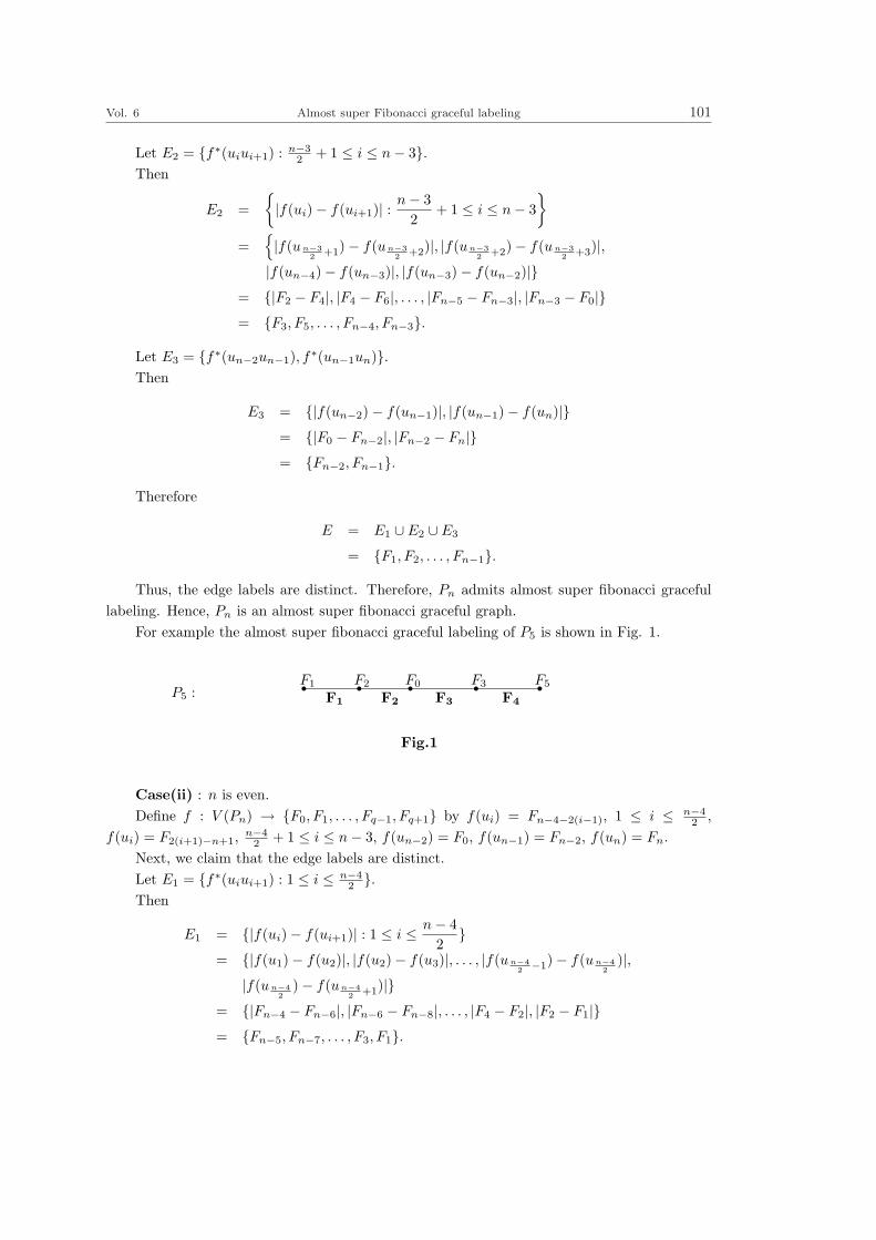
Vol. 6 Almost super Fibonacci graceful labeling 101
Let E2 = f∗(uiui+1) : n−32 + 1 ≤ i ≤ n− 3.
Then
E2 =|f(ui)− f(ui+1)| : n− 3
2+ 1 ≤ i ≤ n− 3
=|f(un−3
2 +1)− f(un−32 +2)|, |f(un−3
2 +2)− f(un−32 +3)|,
|f(un−4)− f(un−3)|, |f(un−3)− f(un−2)|= |F2 − F4|, |F4 − F6|, . . . , |Fn−5 − Fn−3|, |Fn−3 − F0|= F3, F5, . . . , Fn−4, Fn−3.
Let E3 = f∗(un−2un−1), f∗(un−1un).Then
E3 = |f(un−2)− f(un−1)|, |f(un−1)− f(un)|= |F0 − Fn−2|, |Fn−2 − Fn|= Fn−2, Fn−1.
Therefore
E = E1 ∪ E2 ∪ E3
= F1, F2, . . . , Fn−1.
Thus, the edge labels are distinct. Therefore, Pn admits almost super fibonacci gracefullabeling. Hence, Pn is an almost super fibonacci graceful graph.
For example the almost super fibonacci graceful labeling of P5 is shown in Fig. 1.
r r r r rF1 F2 F0 F3 F5
F1 F2 F3 F4P5 :
Fig.1
Case(ii) : n is even.Define f : V (Pn) → F0, F1, . . . , Fq−1, Fq+1 by f(ui) = Fn−4−2(i−1), 1 ≤ i ≤ n−4
2 ,f(ui) = F2(i+1)−n+1, n−4
2 + 1 ≤ i ≤ n− 3, f(un−2) = F0, f(un−1) = Fn−2, f(un) = Fn.Next, we claim that the edge labels are distinct.Let E1 = f∗(uiui+1) : 1 ≤ i ≤ n−4
2 .Then
E1 = |f(ui)− f(ui+1)| : 1 ≤ i ≤ n− 42
= |f(u1)− f(u2)|, |f(u2)− f(u3)|, . . . , |f(un−4
2 −1)− f(un−42
)|,|f(un−4
2)− f(un−4
2 +1)|= |Fn−4 − Fn−6|, |Fn−6 − Fn−8|, . . . , |F4 − F2|, |F2 − F1|= Fn−5, Fn−7, . . . , F3, F1.

102 R. Sridevi, S. Navaneethakrishnan and K. Nagarajan No. 3
Let E2 = f∗(uiui+1) : n−42 + 1 ≤ i ≤ n− 4.
Then
E2 = |f(ui)− f(ui+1)| : n− 42
+ 1 ≤ i ≤ n− 4= |f(un−4
2 +1)− f(un−42 +2)|, |f(un−4
2 +2)− f(un−42 +3)|, . . . ,
|f(un−5)− f(un−4)|, |f(un−4)− f(un−3)|= |F1 − F3|, |F3 − F5|, . . . , |Fn−7 − Fn−5|, |Fn−5 − Fn−3|= F2, F4, . . . , Fn−6, Fn−4.
Let E3 = f∗(un−3un−2), f∗(un−2un−1), f∗(un−1un).Then
E3 = |f(un−3)− f(un−2)|, |f(un−2)− f(un−1)|,|f(un−1)− f(un)|
= |Fn−3 − F0|, |F0 − Fn−2|, |Fn−2 − Fn|= Fn−3, Fn−2, Fn−1.
Therefore
E = E1 ∪ E2 ∪ E3
= F1, F2, . . . , Fn−1.
Thus, the edge labels are distinct. Therefore, Pn admits almost super fibonacci gracefullabeling. Hence, Pn is an almost super fibonacci graceful graph.
For example the almost super fibonacci graceful labeling of P6 is shown in Fig. 2.
r r r r r rF2 F1 F3 F0 F4 F6
F1 F2 F3 F4 F5P6 :
Fig.2.
Definition 2.2. The graph obtained by joining a single pendant edge to each vertex ofpath is called a comb and is denoted by Pn ¯K1 or P+
n .Theorem 2.2. The path P+
n is an almost super fibonacci graceful graph.Proof. Let u1, u2, . . . , un be the vertices of path Pn and v1, v2, . . . , vn be the vertices
adjacent to each vertex of Pn. Also, |V (G)| = 2n and |E(G)| = 2n−1. Define f : V (Pn¯K1) →F0, F1, F2, . . . , Fq−1, Fq+1 by f(ui) = F2i, 1 ≤ i ≤ n − 2, f(vi) = F2i−1, 1 ≤ i ≤ n − 1,f(un−1) = F0, f(un) = F2n−2, f(vn) = F2n.
Next, we claim that the edge labels are distinct.Let E1 = f∗(uiui+1) : i = 1, 2, . . . , n− 3.

Vol. 6 Almost super Fibonacci graceful labeling 103
Then
E1 = |f(ui)− f(ui+1)| : i = 1, 2, . . . , n− 3= |f(u1)− f(u2)|, |f(u2)− f(u3)|, . . . , |f(un−4)− f(un−3)|,
|f(un−3)− f(un−2)|= |F2 − F4|, |F4 − F6|, |F6 − F8|, . . . , |F2n−8 − F2n−6|,
|F2n−6 − F2n−4|= F3, F5, . . . , F2n−7, F2n−5.
Let E2 = f∗(uiui+1) : n− 2 ≤ i ≤ n− 1.Then
E2 = f∗(un−2un−1), f∗(un−1un)= |f(un−2)− f(un−1)|, |f(un−1)− f(un)|= |F2n−4 − F0|, |F0 − F2n−2|= F2n−4, F2n−2.
Let E3 = f∗(u1v1).Then
E3 = |f(u1)− f(v1)|= |F2 − F1|= F1.
Let E4 = f∗(ui+1vi+1) : 1 ≤ i ≤ n− 3.Then
E4 = |f(ui+1)− f(vi+1)| : 1 ≤ i ≤ n− 3= |f(u2 − f(v2)|, |f(u3)− f(v3)|, . . . , |f(un−3)− f(vn−3)|,
|f(un−2)− f(vn−2)|= |F4 − F3|, |F6 − F5|, . . . , |F2n−6 − F2n−7|, |F2n−4 − F2n−5|= F2, F4, . . . , F2n−8, F2n−6.
Let E5 = f∗(un−1vn−1), f∗(unvn).Then
E5 = |f(un−1)− f(vn−1)|, |f(un)− f(vn)|= |F0 − F2n−3|, |F2n − F2n−2|= F2n−3, F2n−1.
Therefore
E = E1 ∪ E2 ∪ E3 ∪ E4 ∪ E5
= F1, F2, . . . , F2n−1.

104 R. Sridevi, S. Navaneethakrishnan and K. Nagarajan No. 3
Thus, the edge labels are distinct. Therefore, Pn ¯ K1 admits almost super fibonaccigraceful labeling. Hence, Pn ¯K1 is an almost super fibonacci graceful graph.
This example shows that the graph P5 ¯K1 is an almost super fibonacci graceful graph.
r r r r r
rrrrr
F2 F4 F6 F0 F8
F10F7F5F3F1
F1 F2 F4 F7 F9
F3 F5 F6 F8
P5 ¯K1 :
Fig.3
Definition 2.3. Let K1,n be a star with n + 1 vertices (n ≥ 2). Adjoin a pendant edge ateach n pendant vertex of K1,n. The resultant graph is called a extension of K1,n and is denotedby K+
1,n.Next, theorem shows that the graph K+
1,n is an almost super Fibonacci graceful graph.Theorem 2.3. The graph G = K+
1,n is an almost super fibonacci graceful graph.Proof. Let (V1, V2) be the bipartion of K1,n, where V1 = u0 and V2 = u1, u2, . . . , un
and v1, v2, . . . , vn be the pendant vertices joined with u1, u2, . . . , un respectively. Also, |V (G)| =2n + 1 and |E(G)| = 2n.
Case(i) : n is odd.Define f : V (G) → F0, F1, F2, . . . , Fq−1, Fq+1 by f(u0) = F0, f(u2i−1) = F4i−3, 1 ≤ i ≤
n+12 , f(u2i) = F4i, 1 ≤ i ≤ n−1
2 , f(v2i−1) = F4i−1, 1 ≤ i ≤ n+12 , f(v2i) = F4i−2, 1 ≤ i ≤ n−1
2 .Next, we claim that the edge labels are distinct.Let E1 = f∗(u0u2i−1): 1 ≤ i ≤ n+1
2 .Then
E1 = |f(u0)− f(u2i−1)| : 1 ≤ i ≤ n + 12
= |f(u0)− f(u1) |, | f(u0)− f(u3)|, . . . , | f(u0)− f(un−2)|, |f(u0)− f(un)|= |F0 − F1|, |F0 − F5|, . . . , |F0 − F2n−5|, |F0 − F2n−1|= F1, F5, . . . , F2n−5, F2n−1.
Let E2 = f∗(u0u2i): 1 ≤ i ≤ n−12 .
Then
E2 = |f(u0)− f(u2i)| : 1 ≤ i ≤ n− 12
= |f(u0)− f(u2)|, |f(u0)− f(u4)|, . . . , |f(u0)− f(un−3)|, |f(u0)− f(un−1)|= |F0 − F4|, |F0 − F8|, . . . , |F0 − F2n−6|, |F0 − F2n−2|= F4, F8, . . . , F2n−6, F2n−2.
Let E3 = f∗(u2i−1v2i−1): 1 ≤ i ≤ n+12 .

Vol. 6 Almost super Fibonacci graceful labeling 105
Then
E3 = |f(u2i−1)− f(v2i−1)| : 1 ≤ i ≤ n + 12
= |f(u1)− f(v1)|, |f(u3)− f(v3)|, . . . , |f(un−2)− f(vn−2)|, |f(un)− f(vn)|= |F1 − F3|, |F5 − F7|, . . . , |F2n−5 − F2n−3|, |F2n−1 − F2n+1|= F2, F6, . . . , F2n−4, F2n.
Let E4 = f∗(u2iv2i): 1 ≤ i ≤ n−12 .
Then
E4 = |f(u2i)− f(v2i)| : 1 ≤ i ≤ n− 12
= |f(u2)− f(v2)|, |f(u4)− f(v4)|, . . . , |f(un−3)− f(vn−3)|,
|f(un−1)− f(vn−1)|= |F4 − F2|, |F8 − F6|, . . . , |F2n−6 − F2n−8|, |F2n−2 − F2n−4|= F3, F7, . . . , F2n−7, F2n−3.
Therefore
E = E1 ∪ E2 ∪ E3 ∪ E4
= F1, F2, . . . , F2n.
Thus, the edge labels are distinct. Therefore, K+1,n admits almost super fibonacci graceful
labeling. Hence, K+1,n is an almost super fibonacci graceful graph.
For example the almost super fibonacci graceful labeling of K+1,5 is shown in Fig. 4.
s
s s s s s
s s s s s
F0
F3 F2 F7 F6 F11
F1 F8 F9F5F4
F1
F2
F9
F10F3 F6
F8F5F4
Fig.4
K+1,5:
F7
Case(ii) : n is even.
Define f : V (G) → F0, F1, F2, . . . , Fq−1, Fq+1 by f(u0) = F0, f(v1) = F1, f(u2i−1) =F4i−2, 1 ≤ i ≤ n
2 , f(u2i) = F4i−1, 1 ≤ i ≤ n2 , f(v2i) = F4i+1, 1 ≤ i ≤ n
2 , f(v2i−1) = F4i−4,2 ≤ i ≤ n
2 .
Next, we claim that the edge labels are distinct.
Let E1 = f∗(u0u2i−1): 1 ≤ i ≤ n2 .

106 R. Sridevi, S. Navaneethakrishnan and K. Nagarajan No. 3
Then
E1 = |f(u0)− f(u2i−1)| : 1 ≤ i ≤ n
2
= |f(u0)− f(u1)|, |f(u0)− f(u3)|, . . . , |f(u0)− f(un−3)|, |f(u0)− f(un−1)|= |F0 − F2|, |F0 − F6|, . . . , |F0 − F2n−6|, |F0 − F2n−2|= F2, F6, . . . , F2n−6, F2n−2.
Let E2 = f∗(u0u2i): 1 ≤ i ≤ n2 .
Then
E2 = |f(u0)− f(u2i)| : 1 ≤ i ≤ n
2
= |f(u0)− f(u2)|, |f(u0)− f(u4)|, . . . , |f(u0)− f(un−2)|, |f(u0)− f(un)|= |F0 − F3|, |F0 − F7|, . . . , |F0 − F2n−5|, |F0 − F2n−1|= F3, F7, . . . , F2n−5, F2n−1.
Let E3 = f∗(u1v1).Then
E3 = |f(u1)− f(v1)|= |F2 − F1|= F1.
Let E4 = f∗(u2i−1v2i−1): 2 ≤ i ≤ n2 .
Then
E4 = |f(u2i−1)− f(v2i−1)| : 2 ≤ i ≤ n
2
= |f(u3)− f(v3)|, |f(u5)− f(v5)|, . . . , |f(un−3)− f(vn−3)|,|f(un−1)− f(vn−1)|
= |F6 − F4|, |F10 − F8|, . . . , |F2n−6 − F2n−8|, |F2n−2 − F2n−4|= F5, F9, . . . , F2n−7, F2n−3.
Let E5= f∗(u2iv2i) : 1 ≤ i ≤ n2 .
Then
E5 = |f(u2i)− f(v2i)| : 1 ≤ i ≤ n
2
= |f(u2)− f(v2)|, |f(u4)− f(v4)|, . . . , |f(un−1)− f(vn−1)|, |f(un)− f(vn)|= |F3 − F5|, |F7 − F9|, . . . , |F2n−5 − F2n−3|, |F2n−1 − F2n+1|= F4, F8, . . . , F2n−4, F2n.
Therefore
E = E1 ∪ E2 ∪ E3 ∪ E4 ∪ E5
= F1, F2, . . . , F2n.

Vol. 6 Almost super Fibonacci graceful labeling 107
Thus, the edge labels are distinct. Therefore, K+1,n admits almost super fibonacci graceful
labeling. Hence, K+1,n is an almost super fibonacci graceful graph.
For example the almost super fibonacci graceful labeling of K+1,4 is shown in Fig. 5.
¡¡
¡¡
@@
@@
r
rrrr
r r r r
F0
F2 F3 F6 F7
F2F3
F6 F7
F1 F5 F4 F9
F1 F4 F5 F8
K+1,4 :
Fig.5
Definition 2.4. The graph G = Fn ⊕P3 consists of a fan Fn and a path P3 of length twowhich is attached with the maximum degree of the vertex of Fn.
Theorem 2.4. G = Fn ⊕ P3 is an almost super fibonacci graceful graph forn ≥ 3.
Proof. Let V (G) = U ∪ V , where U = u0, u1, . . . , un be the vertex set of Fn andV = u0 = v1, v2, v3 be the vertex set of P3. Also, |V (G)| = n+3 and |E(G)| = 2n+1. Definef : V (G) → F0, F1, F2, . . . , Fq−1, Fq+1 by f(u0) = f(v1) = F0, f(ui) = F2i−1, 1 ≤ i ≤ n,f(vi+1) = F2(n+i)−2, 1 ≤ i ≤ 2.
Next, we claim that the edge labels are distinct.Let E1 = f∗(uiui+1): i = 1, 2, · · · , n− 1.Then
E1 = |f(ui)− f(ui+1)| : i = 1, 2, . . . , n− 1= |f(u1)− f(u2)|, |f(u2)− f(u3)|, . . . , |f(un−2)− f(un−1)|,
|f(un−1)− f(un)|= |F1 − F3|, |F3 − F5|, . . . , |F2n−5 − F2n−3|, |F2n−3 − F2n−1|= F2, F4, . . . , F2n−4, F2n−2.
Let E2 = f∗(u0ui): i = 1, 2, · · · , n.Then
E2 = |f(u0)− f(ui)| : i = 1, 2, . . . , n= |F0 − F2i−1| : i = 1, 2, . . . , n= |F0 − F1|, |F0 − F3|, . . . , |F0 − F2n−3|, |F0 − F2n−1|= F1, F3, . . . , F2n−3, F2n−1.
.Let E3=f∗(vivi+1) : i = 1, 2.

108 R. Sridevi, S. Navaneethakrishnan and K. Nagarajan No. 3
Then
E3 = |f(vi)− f(vi+1)| : i = 1, 2= |F0 − F2n+i−1| : i = 1, 2= |F0 − F2n|, |F2n − F2n+2|= F2n, F2n+1.
Therefore
E = E1 ∪ E2 ∪ E3
= F1, F2, . . . , F2n+1.
Thus, the edge labels are distinct. There, Fn ⊕ P3 admits almost super fibonacci gracefullabeling. Hence, Fn ⊕ P3is an almost super fibonacci graceful graph. This example shows thatthe graph F5 ⊕ P3 is an almost super fibonacci graceful graph.
s
s ss s s
s sF0
F1 F3 F5 F7 F9
F10 F12
F1F3 F5 F7
F9
F10 F11
F2 F4 F6 F8
Fig.6
F5 ⊕ P3:
Definition 2.5. An (n, 2t) - graph consists of a cycle of length n with two copies of t-edgepath attached to two adjacent vertices and it is denoted by Cn@2Pt.
Next theorem shows that the (n, 2t) - graph is an almost super Fibonacci graceful graph.Theorem 2.5. The (n, 2t) graph G, where t = 1, n ≡ 0(mod 3) is an almost super
fibonacci graceful graph.Proof. Let u1, u2, . . . , un be the vertices of cycle of length n. Let v, w be the vertices
of paths P1 and P2 joined with u1, un respectively. Also, |V (G)| = |E(G)| = n + 2. DefineDefine f : V (G) → F0, F1, F2, . . . , Fq−1, Fq+1 by f(u1) = F0, f(un) = Fn+1, f(un−1) = Fn−1,f(v) = F1, f(w) = Fn+3. For l = 1, 2, . . . , n−3
3 , f(ui+1) = F2i−3(l−1), 3l − 2 ≤ i ≤ 3l.Next, we claim that the edge labels are distinct. We have to find the edge labeling between
the vertex u1 and starting vertex u2 of the first loop.Let E1 = f∗(u1u2).Then
E1 = |f(u1)− f(u2)|= |F0 − F2|= F2.

Vol. 6 Almost super Fibonacci graceful labeling 109
Let E2 = f∗(ui+1ui+2): 1 ≤ i ≤ 2.For l = 1
Then
E2 = |f∗(ui+1ui+2)| : 1 ≤ i ≤ 2= |f(ui+1)− f(ui+2)| : 1 ≤ i ≤ 2= |f(u2)− f(u3)|, |f(u3)− f(u4)|= |F2 − F4|, |F4 − F6|= F3, F5.
We have to find the edge labeling between the end vertex u4 of the first loop and startingvertex u5 of the second loop.
Let
E12 = f∗(u4u5)
= | f(u4)− f(u5) |= | F6 − F5 |= F4.
For l = 2
Let E3 = f∗(ui+1ui+2) :4 ≤ i ≤ 5.Then
E3 = |f(ui+1 − f(ui+2)| : 4 ≤ i ≤ 5= |f(u5)− f(u6)|, |f(u6)− f(u7)|= |F5 − F7|, |F7 − F9|= F6, F8.
We have to find the edge labeling between the end vertex u7 of the second loop and startingvertex u8 of the third loop.
Let
E13 = f∗(u7u8)
= | f(u7)− f(u8) |= | F9 − F8 |= F7.
etc.,
For l = n−33 − 1
Let En−33 −1 = f∗(ui+1ui+2) : n− 8 ≤ i ≤ n− 7.

110 R. Sridevi, S. Navaneethakrishnan and K. Nagarajan No. 3
Then
En−33 −1 = |f(ui+1)− f(ui+2)| : n− 8 ≤ i ≤ n− 7
= |f(un−7)− f(un−6)|, |f(un−6)− f(un−5)|= |Fn−7 − Fn−5|, |Fn−5 − Fn−3|= Fn−6, Fn−4.
We have to find the edge labeling between the end vertex un−5 of the (n−33 −1)th loop and
starting vertex un−4 of the (n−33 )rd loop.
Let
E1n−3
3 −1= f∗(un−5un−4)= | f(un−5)− f(un−4) |= | Fn−3 − Fn−4 |= Fn−5.
For l = n−33
Let En−33
= f∗(ui+1ui+2): n− 5 ≤ i ≤ n− 4.Then
En−33
= | f(ui+1)− f(ui+2) |: n− 5 ≤ i ≤ n− 4= | f(un−4)− f(un−3) |, | f(un−3)− f(un−2) |= | Fn−4 − Fn−2 |, | Fn−2 − Fn |= Fn−3, Fn−1.
Let E∗ = f∗(un−2un−1), f∗(un−1un), f∗(unu1), f∗(unω), f∗(u1v).Then
E∗ = | f(un−2)− f(un−1) |, | f(un−1)− f(un) |, | f(un)− f(u1) |,| f(un)− f(ω) |, | f(u1)− f(v) |
= | Fn − Fn−1 |, | Fn−1 − Fn+1 |, | Fn+1 − F0 |, | Fn+1 − Fn+3 |, | F0 − F1 |= Fn−2, Fn, Fn+1, Fn+2, F1.
Therefore
E = (E1 ∪ E2∪, . . . , En−33
) ∪ (E12 ∪ E1
3∪, . . . , E1n−3
3 −1) ∪ E∗
= F1, F2, . . . , Fn+1, Fn+2.
Thus, the edge labels are distinct. Therefore, the (n, 2t)-graph admits almost super fi-bonacci graceful labeling. Hence, the (n, 2t)-graph G is an almost super fibonacci gracefulgraph. This example shows that the graph G = (6, 2t) is an almost super fibonacci gracefulgraph.

Vol. 6 Almost super Fibonacci graceful labeling 111
@@
@@¡
¡¡¡
¡¡
¡¡
¡¡
¡¡
¡
@@
@@
r
rr
r
r
r
r
rF0
F2F4
F6
F5 F7
F9
F1
F2
F3
F5
F4
F6
F7
F8
F1G = (6, 2t) :
Fig.7
Definition 2.6. The graph G = C3@2Pn consists of a cycle C3 together with the twocopies of path Pn of length n, two end vertices u1, v1 of Pn is joined with two vertices of C3.
Theorem 2.6. The graph G = C3@2Pn is an almost super Fibonacci graceful graphexcept when n ≡ 2 (mod 3).
Proof. Let V (G) = U ∪V ∪W , where W = w1, w2, w3 be the vertices of C3, U = w1 =u1, u2, . . . , un+1 and V = w2 = v1, v2, . . . , vn+1 be the vertex set of path Pn+1 of length n.Also, |V (G)| = 2n + 3 = |E(G)|.
Case(i) : n ≡ 1 (mod 3).Define f : V (G) → F0, F1, F2, . . . , Fq−1, Fq+1 by f(w3) = Fn+4, when n ≡ 1 (mod 3),
f(un+1−(i−1)) = F2(n−i+3), 1 ≤ i ≤ 2, f(un−1) = F0, f(un−2) = F2n+1, f(un−3) = F2n−1,f(vi) =Fn−i+3, 1 ≤ i ≤ n + 1. For l = 1, 2, . . . , n−4
3 , f(un−3−i) = F2n−2(i−1)+3(l−1), 3l − 2 ≤ i ≤ 3l.Next, we claim that the edge labels are distinct.Let E1 = f∗(un+1un), f∗(unun−1), f∗(un−1un−2), f∗(un−2un−3).Then
E1 = | f(un+1)− f(un) |, | f(un)− f(un−1) |, | f(un−1)− f(un−2) |,| f(un−2)− f(un−3) |
= | F2n+4 − F2n+2 |, | F2n+2 − F0 |, | F0 − F2n+1 |, | F2n+1 − F2n−1 |= F2n+3, F2n+2, F2n+1, F2n.
We have to find the edge labeling between the vertex un−3 and starting vertex un−4 of thefirst loop.
Let E2 = f∗(un−3un−4)Then
E2 = | f(un−3)− f(un−4) |= | F2n−1 − F2n |= F2n−2.

112 R. Sridevi, S. Navaneethakrishnan and K. Nagarajan No. 3
For l = 1Let E3 = f∗(un−3−iun−4−i) : 1 ≤ i ≤ 2Then
E3 = | f(un−3−i)− f(un−4−i) |: 1 ≤ i ≤ 2= | f(un−4)− f(un−5) |, | f(un−5)− f(un−6) |= | F2n − F2n−2 |, | F2n−2 − F2n−4 |= F2n−1, F2n−3.
We have to find the edge labeling between the end vertex un−6 of the first loop and startingvertex un−7 of the second loop.
Let E13 = f∗(un−6un−7)
Then
E13 = | f(un−6)− f(un−7) |
= | F2n−4 − F2n−3 |= F2n−5.
For l = 2Let E4 = f∗(un−3−iun−4−i) : 4 ≤ i ≤ 5)Then
E4 = | f(un−3−i)− f(un−4−i) |: 4 ≤ i ≤ 5= | f(un−7)− f(un−8) |, | f(un−8)− f(un−9) |= | F2n−3 − F2n−5 |, | F2n−5 − F2n−7 |= F2n−4, F2n−6.
We have to find the edge labeling between the end vertex un−9 of the first loop and startingvertex un−10 of the third loop.
Let E14 = f∗(un−9un−10)
Then
E14 = | f(un−9)− f(un−10) |
= | F2n−7 − F2n−6 |= F2n−8.
etc.,For l = n−4
3 − 1Let En−4
3 −1 = f∗(un−3−iun−4−i) : n− 9 ≤ i ≤ n− 8Then
En−43 −1 = | f(un−3−i)− f(un−4−i) |: n− 9 ≤ i ≤ n− 8
= | f(u6)− f(u5) |, | f(u5)− f(u4) |= | Fn+10 − Fn+8 |, | Fn+8 − Fn+6 |= Fn+9, Fn+7.

Vol. 6 Almost super Fibonacci graceful labeling 113
We have to find the edge labeling between the end vertex u6 of the (n−43 − 1)th loop and
starting vertex (n−43 − 1)rd of the third loop.
Let E1n−4
3 −1= f∗(u4u3)
Then
E1n−4
3 −1= | f(u4)− f(u3) |= | Fn+6 − Fn+4 |= Fn+5.
For l = n−43
Let En−43
= f∗(un−3−iun−4−i) : n− 6 ≤ i ≤ n− 5Then
En−43
= |f(un−3−i)− f(un−4−i)| : n− 6 ≤ i ≤ n− 5= |f(u3)− f(u2)|, |f(u2)− f(u1)|= |Fn+7 − Fn+5|, |Fn+5 − Fn+3|= Fn+6, Fn+4.
Let E∗1 = f∗(un+1−(i−1)un−(i−1)) : i = 1
Then
E∗1 = |f(un+1−(i−1))− f(un−(i−1))| : i = 1
= |f(un+1)− f(un)|= |F2n+4 − F2n+2|= F2n+3.
Let E∗2 = f∗(ω1ω3), f∗(ω2ω3), f∗(ω1ω2)
Then
E∗2 = |f(ω1)− f(ω3)|, |f(ω2)− f(ω3)|, |f(ω1)− f(ω2)|
= |Fn+3 − Fn+4|, |Fn+2 − Fn+4|, |Fn+3 − Fn+2|= Fn+2, Fn+3, Fn+1.
Let E∗3 = f∗(vivi+1) : 1 ≤ i ≤ n.
Then
E∗3 = |f(vi)− f(vi+1)| : 1 ≤ i ≤ n
= |f(v1)− f(v2)|, |f(v2)− f(v3)|, . . . , |f(vn−1)− f(vn)|, |f(vn)− f(vn+1)|= |Fn+2 − Fn+1|, |Fn+1 − Fn|, . . . , |F4 − F3|, |F3 − F2|= Fn, Fn−1, . . . , F2, F1.
Therefore
E = (E1 ∪ E2∪, . . . , En−43
) ∪ (E13 ∪ E1
4∪, . . . ,∪E1n−4
3 −1) ∪ (E∗
1 ∪ E∗2 ∪ E∗
3 )
= F1, F2, . . . , F2n+2, F2n+3.

114 R. Sridevi, S. Navaneethakrishnan and K. Nagarajan No. 3
Thus, the edge labels are distinct. Therefore, the graph G = C3@2Pn admits almost superfibonacci graceful labeling. Hence, the graph G = C3@2Pn is an almost super fibonacci gracefulgraph.
For example the almost super fibonacci graceful labeling of C3@2P10 is shown in Fig. 8.
s
s
s s
s s s s s s s s s s
s s s s s s s ss s
F13 F15 F17 F16 F18 F20 F19 F21 F0 F22 F24
F12 F11 F9 F8 F5 F4 F3 F2F10
F12
F13
F14
F10
F16 F15 F17 F19 F18 F20 F21 F22 F23
F9 F8 F7 F5 F4 F3 F2 F1
Fig.8
F11
F6
F7 F6
C3@2P10:
F14
Case(ii): when n ≡ 0 (mod 3)Define f : V (G) → F0, F1, F2, . . . , Fq−1, Fq+1 by f(w3) = Fn+3, when n ≡ 0 (mod 3),
f(un+1−(i−1)) = F2(n−i+3), 1 ≤ i ≤ 2, f(un−1) = F0, f(un−2) = F2n+1, f(un−3) = F2n−1,f(u2) = Fn+6, f(u1) = Fn+4, f(vi) = Fn−i+3, 1 ≤ i ≤ n + 1. For l = 1, 2, . . . , n−6
3 ,f(un−3−i) = F2n−2(i−1)+3(l−1), 3l − 2 ≤ i ≤ 3l.
Next, we claim that the edge labels are distinct.Let E1 = f∗(un+1un), f∗(unun−1), f∗(un−1un−2), f∗(un−2un−3).Then
E1 = | f(un+1)− f(un)|, |f(un)− f(un−1)|, |f(un−1)− f(un−2)|,|f(un−2)− f(un−3)|
= | F2n+4 − F2n+2|, |F2n+2 − F0|, |F0 − F2n+1|, |F2n+1 − F2n−1|= F2n+3, F2n+2, F2n+1, F2n.
We have to find the edge labeling between the vertex un−3 and starting vertex un−4 of thefirst loop.
Let E2 = f∗(un−3un−4)Then
E2 = |f(un−3)− f(un−4)|= |F2n−1 − F2n|= F2n−2.
For l = 1Let E3 = f∗(un−3−iun−4−i) : 1 ≤ i ≤ 2).

Vol. 6 Almost super Fibonacci graceful labeling 115
Then
E3 = |f(un−3−i)− f(un−4−i)| : 1 ≤ i ≤ 2= |f(un−4)− f(un−5)|, |f(un−5)− f(un−6)|= |F2n − F2n−2|, |F2n−2 − F2n−4|= F2n−1, F2n−3.
We have to find the edge labeling between the end vertex un−6 of the first loop and startingvertex un−7 of the second loop.
Let E13 = f∗(un−6un−7)
Then
E13 = |f(un−6)− f(un−7)|
= |F2n−4 − F2n−3|= F2n−5.
For l = 2Let E4 = f∗(un−3−iun−4−i) : 4 ≤ i ≤ 5).Then
E4 = |f(un−3−i)− f(un−4−i)| : 4 ≤ i ≤ 5= |f(un−7)− f(un−8)|, |f(un−8)− f(un−9)|= |F2n−3 − F2n−5|, |F2n−5 − F2n−7|= F2n−4, F2n−6.
We have to find the edge labeling between the end vertex un−9 of the second loop andstarting vertex un−10 of the third loop.
Let E14 = f∗(un−9un−10)
Then
E14 = |f(un−9)− f(un−10)|
= |F2n−7 − F2n−6|= F2n−8.
etc.For l = n−6
3 − 1Let En−6
3 −1 = f∗(un−3−iun−4−i) : n− 11 ≤ i ≤ n− 10.Then
En−63 −1 = |f(un−3−i)− f(un−4−i)| : n− 11 ≤ i ≤ n− 10
= |f(u8)− f(u7)|, |f(u7)− f(u6)|= |Fn+12 − Fn+10|, |Fn+10 − Fn+8|= Fn+11, Fn+9.

116 R. Sridevi, S. Navaneethakrishnan and K. Nagarajan No. 3
We have to find the edge labeling between the end vertex u6 of the (n−63 − 1)th loop and
starting vertex u5 of the (n−63 )rd loop.
Let E1n−6
3 −1= f∗(u6u5).
Then
E1n−6
3 −1= |f(u6)− f(u5)|= |Fn+8 − Fn+9|= Fn+7.
For l = n−63
Let En−63
= f∗(un−3−iun−4−i) : n− 8 ≤ i ≤ n− 7.Then
En−63
= |f(un−3−i)− f(un−4−i)| : n− 8 ≤ i ≤ n− 7= |f(u5)− f(u4)|, |f(u4)− f(u3)|= |Fn+9 − Fn+7|, |Fn+7 − Fn+5|= Fn+8, Fn+6.
We have to find the edge labeling between the end vertex u3 of the (n−63 )th loop and the
vertex u2.Let
E∗1 = f∗(u3u2)
= |f(u3)− f(u2)|= |Fn+5 − Fn+6|= Fn+4.
Let E∗2 = f∗(u2u1), f∗(ω1ω3), f∗(ω2ω3), f∗(ω1ω2).
Then
E∗2 = |f(u2)− f(u1)|, |f(ω1)− f(ω3)|, |f(ω2)− f(ω3)|, |f(ω1)− f(ω2)|
= |Fn+6 − Fn+4|, |Fn+4 − Fn+3|, |Fn+2 − Fn+3|, |Fn+4 − Fn+2|= Fn+5, Fn+2, Fn+1, Fn+3.
Let E∗3 = f∗(vivi+1) : 1 ≤ i ≤ n.
Then
E∗3 = |f(vi)− f(vi+1)| : 1 ≤ i ≤ n
= |f(v1)− f(v2)|, |f(v2)− f(v3)|, . . . , |f(vn−1)− f(vn)|, |f(vn)− f(vn+1)|= |Fn+2 − Fn+1|, |Fn+1 − Fn|, . . . , |F4 − F3|, |F3 − F2|= Fn, Fn−1, . . . , F2, F1.
Therefore
E = (E1 ∪ E2∪, . . . , En−63
) ∪ (E13 ∪ E1
4∪, . . . , E1n−6
3 −1) ∪ (E∗
1 ∪ E∗2 ∪ E∗
3 )
= F1, F2, . . . , F2n+2, F2n+3.

Vol. 6 Almost super Fibonacci graceful labeling 117
Thus, the edge labels are distinct. Therefore, the graph G = C3@2Pn admits almost superfibonacci graceful labeling. Hence, the graph G = C3@2Pn is an almost super fibonacci gracefulgraph.
For example the almost super fibonacci graceful labeling of C3@2P9 is shown in Fig.9.
s s
s
s s
s
s sssssss
s s s s s s s s
F13 F15 F14 F16 F18 F22F20F0F19F17
F12
F11 F10 F9 F8 F7 F6 F5 F4 F3 F2
Fig.9
F14 F13 F15 F17 F16 F18 F19 F20 F21
F9 F8 F7 F6 F5 F4 F3 F2 F1
C3@2P9:
F10
F12
F11
Definition 2.7. The graph G = C3n+1 ªK1,2 consists of a cycle C3n+1 of length 3n + 1and K1,2 is attached with the vertex un of C3n+1.
The following theorem shows that the graph G = C3n+1ªK1,2 is an almost super fibonaccigraceful graph.
Theorem 2.7. The graph G = C3n+1 ªK1,2 is an almost super fibonacci graceful graph.Proof. Let V (G) = V1 ∪ V2, where V1 = u1, u2, . . . , un be the vertex set of C3n+1 and
V2 = v, w be the end vertices of K1,2. Also, |V (G)| = |E(G)| = n + 2.Define f : V (G) → F0, F1, F2, . . . , Fq−1, Fq+1 by f(ui) = F2(i−1), 1 ≤ i ≤ 2, f(ui) =
F2i−3, 3 ≤ i ≤ 4, f(v) = Fn, f(w) = Fn+3. For l = 1, 2, . . . , n−43 , f(ui+4) = F2i−3l+5,
3l − 2 ≤ i ≤ 3l.Next, we claim that the edge labels are distinct.Let E1 = f∗(uiui+1) : 1 ≤ i ≤ 3.Then
E1 = |f(ui)− f(ui+1)| : 1 ≤ i ≤ 3= |f(u1)− f(u2)|, |f(u2)− f(u3)|, |f(u3)− f(u4)|= |F0 − F2|, |F2 − F3|, |F3 − F5|= F2, F1, F4.
We have to find the edge labeling between the vertex u4 and starting vertex u5 of the firstloop.
Let E2 = f∗(u4u5).Then
E2 = |f(u4)− f(u5)|= |F5 − F4|= F3.

118 R. Sridevi, S. Navaneethakrishnan and K. Nagarajan No. 3
For l = 1Let E3 = f∗(ui+4ui+5) : 1 ≤ i ≤ 2.Then
E3 = |f(ui+4)− f(ui+5)| : 1 ≤ i ≤ 2= |f(u5)− f(u6)|, |f(u6)− f(u7)|= |F4 − F6|, |F6 − F8|= F5, F7.
We have to find the edge labeling between the end vertex u7 of the first loop and startingvertex u8 of the second loop.
Let E(1)3 = f∗(u7u8).
Then
E(1)3 = |f(u7)− f(u8)|
= |F8 − F7|= F6.
For l = 2Let E4 = f∗(ui+4ui+5) : 4 ≤ i ≤ 5.Then
E4 = |f(ui+4)− f(ui+5)| : 4 ≤ i ≤ 5= |f(u8)− f(u9)|, |f(u9)− f(u10)|= |F7 − F9|, |F9 − F11|= F8, F10.
We have to find the edge labeling between the end vertex u10 of the second loop andstarting vertex u11 of the third loop.
Let E(1)4 = f∗(u10u11).
Then
E(1)4 = |f(u10)− f(u11)|
= |F11 − F10|= F9.
etc.For l = n−4
3 − 1Let En−4
3 −1 = f∗(ui+4ui+5) : n− 9 ≤ i ≤ n− 8.Then
En−43 −1 = |f(ui+4)− f(ui+5)| : n− 9 ≤ i ≤ n− 8
= |f(un−5)− f(un−4)|, |f(un−4)− f(un−3)|= |Fn−6 − Fn−4|, |Fn−4 − Fn−2|= Fn−5, Fn−3.

Vol. 6 Almost super Fibonacci graceful labeling 119
We have to find the edge labeling between the end vertex un−3 of the (n−43 −1)th loop and
starting vertex un−2 of the (n−43 )rd loop.
Let E(1)n−4
3 −1= f∗(un−3un−2).
Then
E(1)n−4
3 −1= |f(un−3)− f(un−2)|= |Fn−2 − Fn−3|= Fn−4.
For l = n−43
Let En−43
= f∗(ui+4ui+5) : n− 6 ≤ i ≤ n− 5.Then
En−43
= |f(ui+4)− f(ui+5)| : n− 6 ≤ i ≤ n− 5= |f(un−2)− f(un−1)|, |f(un−1)− f(un)|= |Fn−3 − Fn−1|, |Fn−1 − Fn+1|= Fn−2, Fn.
Let E∗ = f∗(unu1), f∗(unv), f∗(unw).Then
E∗ = |f(un)− f(u1)|, |f(un)− f(v)|, |f(un)− f(w)|= |Fn+1 − F0|, |Fn+1 − Fn|, |Fn+1 − Fn+3|= Fn+1, Fn−1, Fn+2.
Theorefore
E = (E1 ∪ E2, . . . ,∪En−43
) ∪ (E(1)3 ∪ E
(1)4 ∪, . . . ,∪E
(1)n−4
3 −1) ∪ E∗
= F1, F2, . . . , Fn+1, Fn+2.Thus, the edge labels are distinct. Therefore, C3n+1 ªK1,2 admits almost super fibonacci
graceful labeling. Hence, C3n+1 ªK1,2 is an almost super fibonacci graceful graph.This example shows that the graph C7 ªK1,2 is an almost super fibonacci graceful graph.
s
s
s
s
s
s
s
s
F10
F7
F0
F3
F5
F4
F6
s
F2
F7
F5
F3
F1
F2
F8
F4
F8
F9
F6
Fig.10
C7 ªK1,2:

120 R. Sridevi, S. Navaneethakrishnan and K. Nagarajan No. 3
Definition 2.8. G = K1,n ® K1,2 is a graph in which K1,2 is joined with each pendantvertex of K1,n.
Theorem 2.8. The graph G = K1,n ®K1,2 is an almost super Fibonacci graceful graph.Proof. Let u0, u1, u2, . . . , un be the vertex set of K1,n and v1, v2, . . . , vn and w1, w2, . . . , wn
be the vertices joined with the pendant vertices u1, u2, . . . , un of K1,n respectively. Also,|V (G)| = 3n + 1 and |E(G)| = 3n.
Define f : V (G) → F0, F1, F2, . . . , Fq−1, Fq+1 by f(u0) = F0, f(ui) = F3i−1, 1 ≤ i ≤ n,f(vi) = F3i, 1 ≤ i ≤ n, f(wi) = F3i+1, 1 ≤ i ≤ n.
Next, we claim that the edge labels are distinct.Let E1 = f∗(u0ui) : i = 1, 2, . . . , n.Then
E1 = |f(u0)− f(ui)| : i = 1, 2, . . . n= |f(u0)− f(u1)|, |f(u0)− f(u2)|, . . . , |f(u0)− f(un−1)|, |f(u0)− f(un)|= |F0 − F2|, |F0 − F5|, . . . , |F0 − F3n−4|, |F0 − F3n−1|= F2, F5, . . . , F3n−4, F3n−1.
Let E2 = f∗(uivi) : i = 1, 2, . . . n.Then
E2 = |f(ui)− f(vi)| : i = 1, 2, . . . , n= |f(u1)− f(v1)|, |f(u2)− f(v2)|, . . . , |f(un−1)− f(vn−1)|, |f(un)− f(vn)|= |F2 − F3|, |F5 − F6|, . . . , |F3n−4 − F3n−3|, |F3n−1 − F3n|= F1, F4, . . . , F3n−5, F3n−2.
Let E3 = f∗(uiwi) : i = 1, 2, . . . n .Then
E3 = |f(ui)− f(wi)| : i = 1, 2, . . . , n= |f(u1)− f(w1)|, |f(u2)− f(w2)|, . . . , |f(un−1)− f(wn−1)|, |f(un)− f(wn)|= |F2 − F4|, |F5 − F7|, . . . , |F3n−4 − F3n−2|, |F3n−1 − F3n+1|= F3, F6, . . . , F3n−3, F3n.
Theorefore
E = E1 ∪ E2 ∪ E3
= F1, F2, . . . , F3n.
Thus, the edge labels are distinct. Therefore, K1,n ®K1,2 admits almost super fibonaccigraceful labeling. Hence, K1,n ®K1,2 is an almost super fibonacci graceful graph.
This example shows that the graph K1,3®K1,2 is an almost super fibonacci graceful graph.

Vol. 6 Almost super Fibonacci graceful labeling 121
s
s
s s s s
s s
s s
F0
F2
F3 F4 F6 F9F7
F5 F8
F8F5
F2
F1F3 F4 F6 F7 F9
Fig.11
K1,3 ®K1,2:
F10
Definition 2.9. Let u, v be the center vertices of B2,n. Let u1, u2 be the vertices joinedwith u and v1, v2, . . . , vn be the vertices joined with v. Let w1, w2, . . . , wn be the vertices of thesubdivision of edges vvi (1 ≤ i ≤ n) respectively and it is denoted by (B2,n : wi), 1 ≤ i ≤ n.
Theorem 2.9. The graph G = (B2,n : wi), 1 ≤ i ≤ n, where n ≥ 2 is an almost superfibonacci graceful graph.
Proof. Let u, v be the center vertices of B2,n. Let u1, u2 be the vertices joined with u andv1, v2, . . . , vn be the vertices joined with v and w1, w2, . . . , wn be the vertices of the subdivisionof edges vvi (1 ≤ i ≤ n) respectively. Also, |V (G)| = 2n + 4 and |E(G)| = 2n + 3.
Case(i) : n is odd.
Define f : V (G) → F0, F1, F2, . . . , Fq−1, Fq+1 by f(u) = F2n+2, f(u1) = F2n+4, f(u2) =F2n, f(v) = F0, f(v2i−1) = F2n−4i+5, 1 ≤ i ≤ n+1
2 ,f(v2i) = F2n−4i, 1 ≤ i ≤ n−12 ,
f(w2i−1) = F2n−4i+3, 1 ≤ i ≤ n+12 , f(w2i) = F2n−4i+2, 1 ≤ i ≤ n−1
2 .
Next, we claim that the edge labels are distinct.
Let E1 = f∗(uui) : 1 ≤ i ≤ 2.Then
E1 = |f(u)− f(ui)| : 1 ≤ i ≤ 2= |f(u)− f(u1)|, |f(u)− f(u2)|= |F2n+2 − F2n+4|, |F2n+2 − F2n|= F2n+3, F2n+1.
Let E2 = f∗(uv).Then
E2 = |f(u)− f(v)|= |F2n+2 − F0|= F2n+2.
Let E3 = f∗(vw2i−1) : 1 ≤ i ≤ n+12 .

122 R. Sridevi, S. Navaneethakrishnan and K. Nagarajan No. 3
Then
E3 = |f(v)− f(w2i−1)| : 1 ≤ i ≤ n + 12
= |f(v)− f(w1)|, |f(v)− f(w3)|, . . . , |f(v)− f(wn−2)|, |f(v)− f(wn)|= |F0 − F2n−1|, |F0 − F2n−5|, . . . , |F0 − F5|, |F0 − F1|= F2n−1, F2n−5, . . . , F5, F1.
Let E4 = f∗(vw2i) : 1 ≤ i ≤ n−12 .
Then
E4 = |f(v)− f(w2i)| : 1 ≤ i ≤ n− 12
= |f(v)− f(w2)|, |f(v)− f(w4)|, . . . , |f(v)− f(wn−3)|, |f(v)− f(wn−1)|= |F0 − F2n−2|, |F0 − F2n−6|, . . . , |F0 − F8|, |F0 − F4|= F2n−2, F2n−6, . . . , F8, F4.
Let E5 = f∗(v2i−1w2i−1) : 1 ≤ i ≤ n+12 .
Then
E5 = |f(v2i−1)− f(w2i−1)| : 1 ≤ i ≤ n + 12
= |f(v1)− f(w1)|, |f(v3)− f(w3)|, . . . , |f(vn−2)− f(wn−2)|, |f(vn)− f(wn)|= |F2n+1 − F2n−1|, |F2n−3 − F2n−5|, . . . , |F7 − F5|, |F3 − F1|= F2n, F2n−4, . . . , F6, F2.
Let E6 = f∗(v2iw2i) : 1 ≤ i ≤ n−12 .
Then
E6 = |f(v2i)− f(w2i)| : 1 ≤ i ≤ n− 12
= |f(v2)− f(w2)|, |f(v4)− f(w4)|, . . . , |f(vn−3)− f(wn−3)|,
|f(vn−1)− f(wn−1)|= |F2n−4 − F2n−3|, |F2n−8 − F2n−6|, . . . , |F6 − F8|, |F2 − F4|= F2n−3, F2n−7, . . . , F7, F3.
Theorefore, E = E1 ∪ E2 ∪ E3 ∪ E4 ∪ E5 ∪ E6 = F1, F2 . . . F2n+3.Thus, the edge labels are distinct. Therefore, the graph (B2,n : wi), 1 ≤ i ≤ n admits
almost super fibonacci graceful labeling. Hence, (B2,n : wi), 1 ≤ i ≤ n is an almost superfibonacci graceful graph.
For example the almost super fibonacci graceful labeling of B2,5 is shown in Fig. 12.

Vol. 6 Almost super Fibonacci graceful labeling 123
s s
s
s
s
ss
s
sF14
F10
F0
F11
F6
F7
F2
F3
F13
F11
F12
sss
ss
F9F8
F4
F1
F9
F10
F1
F2
F3
F6
F4
F5
F8
F6
F12B2,5:
Fig.12
F7
F5
Case(ii) : n is even.
Define f : V (G) → F0, F1, F2, . . . , Fq−1, Fq+1 by f(u) = F2n+2, f(u1) = F2n+4, f(u2) =F2n, f(v) = F0, f(vn) = F1, f(v2i−1) = F2n−4i+5, 1 ≤ i ≤ n
2 , f(v2i) = F2n−4i, 1 ≤ i ≤ n2 − 1,
f(w2i−1) = F2n−4i+3, 1 ≤ i ≤ n2 , f(w2i) = F2n−4i+2, 1 ≤ i ≤ n
2 .
Next, we claim that the edge labels are distinct.
Let E1 = f∗(uui) : 1 ≤ i ≤ 2.Then
E1 = |f(u)− f(ui)| : 1 ≤ i ≤ 2= |f(u)− f(u1)|, |f(u)− f(u2)|= |F2n+2 − F2n+4|, |F2n+2 − F2n|= F2n+3, F2n+1.
Let E2 = f∗(uv).Then
E2 = |f(u)− f(v)|= |F2n+2 − F0|= F2n+2.
Let E3 = f∗(vw2i−1) : 1 ≤ i ≤ n2
Then
E3 = |f(v)− f(w2i−1)| : 1 ≤ i ≤ n
2
= |f(v)− f(w1)|, |f(v)− f(w3)|, . . . , |f(v)− f(wn−3)|, |f(v)− f(wn−1)|= |F0 − F2n−1|, |F0 − F2n−5|, . . . , |F0 − F7|, |F0 − F3|= F2n−1, F2n−5, . . . , F7, F3.
Let E4 = f∗(vw2i) : 1 ≤ i ≤ n−12
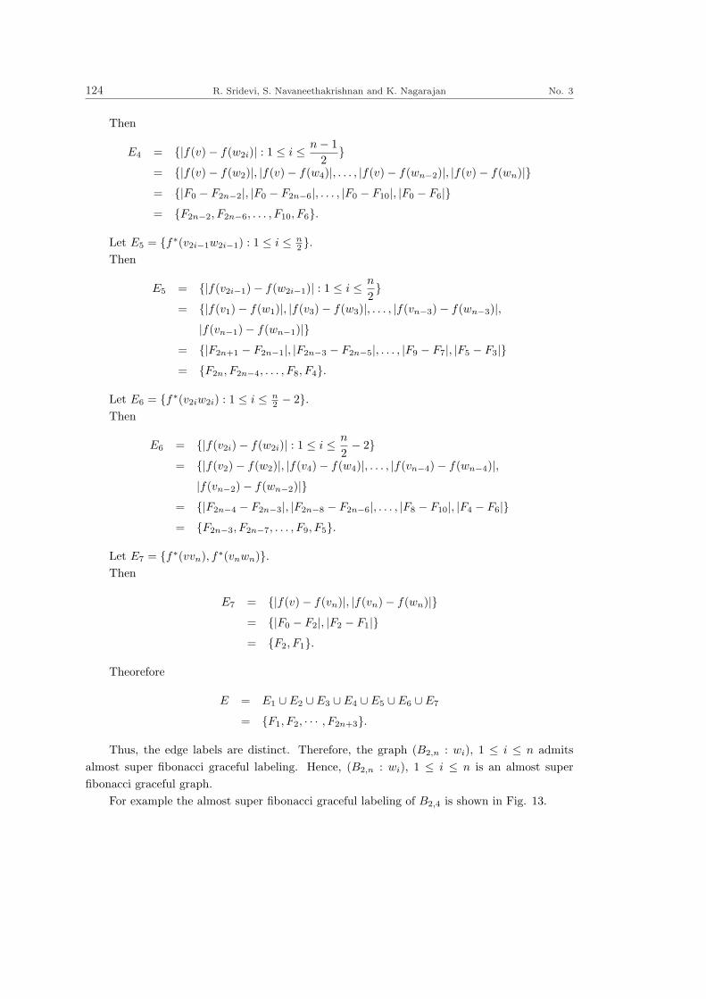
124 R. Sridevi, S. Navaneethakrishnan and K. Nagarajan No. 3
Then
E4 = |f(v)− f(w2i)| : 1 ≤ i ≤ n− 12
= |f(v)− f(w2)|, |f(v)− f(w4)|, . . . , |f(v)− f(wn−2)|, |f(v)− f(wn)|= |F0 − F2n−2|, |F0 − F2n−6|, . . . , |F0 − F10|, |F0 − F6|= F2n−2, F2n−6, . . . , F10, F6.
Let E5 = f∗(v2i−1w2i−1) : 1 ≤ i ≤ n2 .
Then
E5 = |f(v2i−1)− f(w2i−1)| : 1 ≤ i ≤ n
2
= |f(v1)− f(w1)|, |f(v3)− f(w3)|, . . . , |f(vn−3)− f(wn−3)|,|f(vn−1)− f(wn−1)|
= |F2n+1 − F2n−1|, |F2n−3 − F2n−5|, . . . , |F9 − F7|, |F5 − F3|= F2n, F2n−4, . . . , F8, F4.
Let E6 = f∗(v2iw2i) : 1 ≤ i ≤ n2 − 2.
Then
E6 = |f(v2i)− f(w2i)| : 1 ≤ i ≤ n
2− 2
= |f(v2)− f(w2)|, |f(v4)− f(w4)|, . . . , |f(vn−4)− f(wn−4)|,|f(vn−2)− f(wn−2)|
= |F2n−4 − F2n−3|, |F2n−8 − F2n−6|, . . . , |F8 − F10|, |F4 − F6|= F2n−3, F2n−7, . . . , F9, F5.
Let E7 = f∗(vvn), f∗(vnwn).Then
E7 = |f(v)− f(vn)|, |f(vn)− f(wn)|= |F0 − F2|, |F2 − F1|= F2, F1.
Theorefore
E = E1 ∪ E2 ∪ E3 ∪ E4 ∪ E5 ∪ E6 ∪ E7
= F1, F2, · · · , F2n+3.
Thus, the edge labels are distinct. Therefore, the graph (B2,n : wi), 1 ≤ i ≤ n admitsalmost super fibonacci graceful labeling. Hence, (B2,n : wi), 1 ≤ i ≤ n is an almost superfibonacci graceful graph.
For example the almost super fibonacci graceful labeling of B2,4 is shown in Fig. 13.

Vol. 6 Almost super Fibonacci graceful labeling 125
s
s
s
s
s
s
s
s
sss
s
F12
F8
F10 F0
F9
F4
F5
F1
F7F11
F9
F8
F7 F5F6
F1
F2
F10
Fig.13
B2,4 :
F2
F3 F4F3
F6
References
[1] R. Frucht, Nearly graceful labelings of graphs, Scientia, 5(1992-1993), 47-59.[2] G. J. Gallian, A Dynamic survey of graph labeling, The electronic Journal of Combino-
torics, 16(2009), 219.[3] Ian Anderson, A first course in combinatorial Mathematics, Claridon Press-Oxford,
28(1989), 3-13.[4] K. M. Kathiresan and S. Amutha, Fibonacci graceful graphs, Ph. D. Thesis, Madurai
Kamaraj University, October 2006.[5] D. Moulton, Graceful labelings of triangular snakes, Ars Combin, 28(1989), 3-13.[6] A. Rosa, On certain valuations of the vertices of a graph, Theory of graphs (International
Symposium), Rome, 7(1966).

Top Related