


Languages
Pages
Legal


i
VLSI IMPLEMENTATION OF BLOCK
ERROR CORRECTION CODING
TECHNIQUES
A thesis submitted for the degree of Bachelors of Technology.
National Institute of Technology, Rourkela,
By
RAJEEV KUMAR-107EI003 ABHISHEK GUPTA-107EC007
Under the guidance of
Prof. S.K. Patra
Department of Electronics and Communication Engineering National Institute of Technology
Rourkela Orissa May, 2011

ii
CERTIFICATE
This is to certify that the work in this thesis entitled “VLSI Implementation
of Block Error Correction Coding Techniques” submitted by Rajeev Kumar
(Roll No. 107EI003) and Abhishek Gupta (Roll No. 107EC007) has been carried
out under my supervision in partial fulfillment of the requirements for the degree
of Bachelor of Technology during session 2007-2011 in the Department of
Electronics and Communication Engineering, National Institute of Technology,
Rourkela, and this work has not been submitted elsewhere for a degree.
Place: ROURKELA Prof. S. K. Patra
Date: 16th
may 2011 H.O.D, Dept. of ECE
NIT Rourkela
iii
Acknowledgement
On the submission of our Thesis report of “VLSI Implementation of Block
Error Correction Coding Techniques”, we would like to extend our gratitude &
sincere thanks to our mentor Prof. Sarat Kumar Patra, H.O.D of the Department
of Electronics and Communication Engineering, for his constant motivation and
support during the course of our work. We would like to sincerely thank him for
his patience and guidance in providing us a clear understanding about the intricate
details of the topic and strengthening the foundation throughout the work.
Also we would like to thank Mr. Ayaskanta Swain and Mr. Bijay Sharma whose
contribution in this project is quite significant. Finally, a word of thanks to all the
faculty members of Department of Electronics and Communication Engineering,
for their generous help in various ways for overall completion of our thesis.
Rajeev Kumar Abhishek Gupta
107EI003 107EC007
iv
Abstract
Communication Engineering has become the most vital field of Engineering in today‟s
life. The world is dreaded to think beyond any communication gadgets. Data communication
basically involves transfers of data from one place to another or from one point of time to
another. Error may be introduced by the channel which makes data unreliable for user. Hence we
need different error detection and error correction schemes.
In the present work, we perform the comparative study between different FECs like
Turbo codes, Reed-Solomon codes and LPDC codes. But among all these we find Reed Solomon
to be most efficient for data communication because of low coding complexity and high coding
rate. The RS codes are non-binary, linear and cyclic codes used for burst error correction. They
are used in numerous applications like CDs, DVDs and deep space communication. We simulate
RS Encoder and RS Decoder for double error correcting RS (7, 3) code. Then we implement RS
(255,239) code in VHDL. In RS (255,239) code, each data symbol consists of 8 bits which is
quite practical as most of the data transfer is done in terms of bytes. The implementation has
been done in the most efficient algorithms to optimize the design in terms of space utilization
and latency of the code. The behavioral simulation has been carried out for each block and for
the whole design also. Finally, the FPGA utilization and clock cycles needed are analyzed and
compared with the already developed designs.

v
Contents
1. Introduction:
1.1 Communication Process . . . . . . . . . . . . . . . . . . . . . . . . . . . . . . . . . . . . . . . . . . . . . . . 1
1.2 Error Correction Schemes . . . . . . . . . . . . . . . . . . . . . . . . . . . . . . . . . . . . . . . . . . . . . .1
2. Communication System
2.1 Introduction . . . . . . . . . . . . . . . . . . . . . . . . . . . . . . . . . . . . . . . . . . . . . . . . . . . . . . . . . . . 4
2.2 Communication Channel . . . . . . . . . . . . . . . . . . . . . . . . . . . . . . . . . . . . . . . . . . . . . . . . . 5
3. Coding Schemes
3.1 Definitions . . . . . . . . . . . . . . . . . . . . . . . . . . . . . . . . . . . . . . . . . . . . . . . . . . . . . . . . . . . . .6
3.2 Error Detection Schemes . . . . . . . . . . . . . . . . . . . . . . . . . . . . . . . . . . . . . . . . . . . . . . . . . .7
3.3 Comparative Study between various FECS . . . . . . . . . . . . . . . . . . . . . . . . . . . . . . . . . . . 8
4. Finite Fields
4.1 Definitions . . . . . . . . . . . . . . . . . . . . . . . . . . . . . . . . . . . . . . . . . . . . . . . . . . . . . . . . . . . . 10
4.2 Galois Fields . . . . . . . . . . . . . . . . . . . . . . . . . . . . . . . . . . . . . . . . . . . . . . . . . . . . . . . . . . .11

vi
4.3 Primitive Polynomial . . . . . . . . . . . . . . . . . . . . . . . . . . . . . . . . . . . . . . . . . . . . . . . . . . . . 12
5. Reed Solomon Codes
5.1 Introduction . . . . . . . . . . . . . . . . . . . . . . . . . . . . . . . . . . . . . . . . . . . . . . . . . . . . . . . . . . 14
5.2 Reed Solomon Error Probability . . . . . . . . . . . . . . . . . . . . . . . . . . . . . . . . . . . . . . . . . . 15
5.3 RS Encoder . . . . . . . . . . . . . . . . . . . . . . . . . . . . . . . . . . . . . . . . . . . . . . . . . . . . . . . . .. . 18
5.4 RS Decoder . . . . . . . . . . . . . . . . . . . . . . . . . . . . . . . . . . . . . . . . . . . . . . . . . . . . . . . . . . .19
5.5 MATLAB Simulation of (7,3) RS code . . . . . . . . . . . . . . . . . . . . . . . . . . . . . . . . . . . . . 20
6. GF Implementation for RS (255,239) code
In VHDL
6.1 Introduction . . . . . . . . . . . . . . . . . . . . . . . . . . . . . . . . . . . . . . . . . . . . . . . . . . . . . . . . . 22
6.2 GF Multiplier . . . . . . . . . . . . . . . . . . . . . . . . . . . . . . . . . . . . . . . . . . . . . . . . . . . . . . . . 22
6.3 GF Elements . . . . . . . . . . . . . . . . . . . . . . . . . . . . . . . . . . . . . . . . . . . . . . . . . . . . . . . . .27
6.4 Generator Polynomial . . . . . . . . . . . . . . . . . . . . . . . . . . . . . . . . . . . . . . . . . . . . . . . . . . 27
6.5 GF Element Inversion Block . . . . . . . . . . . . . . . . . . . . . . . . . . . . . . . . . . . . . . . . . . . . .27
7. RS Encoder Design
7.1 General Description . . . . . . . . . . . . . . . . . . . . . . . . . . . . . . . . . . . . . . . . . . . . . . . . . . . . .29
7.2 Design Details . . . . . . . . . . . . . . . . . . . . . . . . . . . . . . . . . . . . . . . . . . . . . . . . . . . . . . . . . 31
8. RS Decoder Design
8.1 Introduction . . . . . . . . . . . . . . . . . . . . . . . . . . . . . . . . . . . . . . . . . . . . . . . . . . . . . . . . . . .33

vii
8.2 Design Details . . . . . . . . . . . . . . . . . . . . . . . . . . . . . . . . . . . . . . . . . . . . . . . . . . . . . . . . .35
9. Results and Conclusion
9.1 Results . . . . . . . . . . . . . . . . . . . . . . . . . . . . . . . . . . . . . . . . . . . . . . . . . . . . . . . . . . . . . . . 42
9.2 Conclusion and Future Work . . . . . . . . . . . . . . . . . . . . . . . . . . . . . . . . . . . . . . . . . . . . . .43

viii
List of Figures
2.1 Block Diagram of Communication System . . . . . . . . . . . . . . . . . . . . . . . . . . . . . . . . . . 4
5.1 PB versus the channel-symbol probability p . . . . . . . . . . . . . . . . . . . . . . . . . . . . . . . . . . 16
5.2 Bit-error probability versus Eb/N0 . . . . . . . . . . . . . . . . . . . . . . . . . . . . . . . . . . . . . . . . . 17
5.3 MATLAB simulation of RS(7, 3) code . . . . . . . . . . . . . . . . . . . . . . . . . . . . . . . . . . . . . 21
6.1 GF multiplier . . . . . . . . . . . . . . . . . . . . . . . . . . . . . . . . . . . . . . . . . . . . . . . . . . . . . . . . . 26
6.2 Behavioural simulation of GF multiplier . . . . . . . . . . . . . . . . . . . . . . . . . . . . . . . . . . . . 26
7.1 RS encoder architecture . . . . . . . . . . . . . . . . . . . . . . . . . . . . . . . . . . . . . . . . . . . . . . . . . 30
7.2 RS encoder block diagram . . . . . . . . . . . . . . . . . . . . . . . . . . . . . . . . . . . . . . . . . . . . . . . 30
7.3 RTL schematic of the encoder 1st part containing 16 redundant symbols generator . . . 32
7.4 RTL schematic of the encoder 2nd
part containing multiplexers . . . . . . . . . . . . . . . . . . . 32
7.5 Behavioural simulation of the encoder showing only first few clock cycles . . . . . . . . . .32
8.1 RS decoder block . . . . . . . . . . . . . . . . . . . . . . . . . . . . . . . . . . . . . . . . . . . . . . . . . . . . . . 34
8.2 Functional block diagram of decoder . . . . . . . . . . . . . . . . . . . . . . . . . . . . . . . . . . . . . . . 35
8.3 RS syndrome generator . . . . . . . . . . . . . . . . . . . . . . . . . . . . . . . . . . . . . . . . . . . . . . . . . . .37
8.4 A Part of RTL schematic of Error Evaluator Polynomial Generator . . . . . . . . . . . . . . . . 39
8.5 A Part of RTL schematic of Error Evaluator . . . . . . . . . . . . . . . . . . . . . . . . . . . . . . . . . . .41
ix
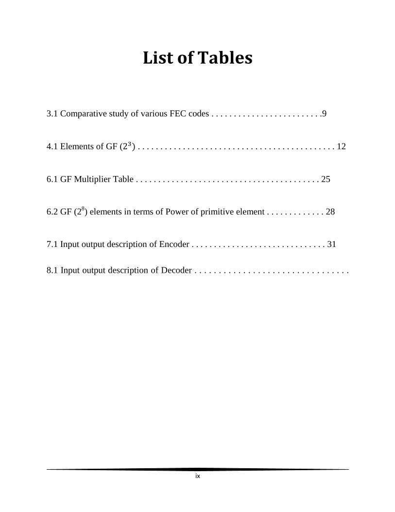
List of Tables
3.1 Comparative study of various FEC codes . . . . . . . . . . . . . . . . . . . . . . . . .9
4.1 Elements of GF ( . . . . . . . . . . . . . . . . . . . . . . . . . . . . . . . . . . . . . . . . . . . . 12
6.1 GF Multiplier Table . . . . . . . . . . . . . . . . . . . . . . . . . . . . . . . . . . . . . . . . . 25
6.2 GF (28) elements in terms of Power of primitive element . . . . . . . . . . . . . 28
7.1 Input output description of Encoder . . . . . . . . . . . . . . . . . . . . . . . . . . . . . . 31
8.1 Input output description of Decoder . . . . . . . . . . . . . . . . . . . . . . . . . . . . . . . .

1
Chapter 1
INTRODUCTION
1.1 Communication Process
Today Communication Engineering has become the vital field of engineering. Over the
past few decades the whole world has been enrolled by communication gadgets whether it is
television, radio, atm or any other communication system. We all will be dreaded to think world
beyond communication. Communication basically involves transfers and reception of
information from one place to another place or from one point of time to another point of time.
In doing so there may be situations that error may be encountered in the channel due to various
factors like Electromagnetic Interferences, Cross talk and Bandwidth limitation etc. Reliability
and Efficiency are the two important goals which are to be achieved by all the advancement in
the field of communication theory. Reliability refers to the reception of the correct information
that was sent through the channel and efficiency refers to the speed of transmission, transceiver‟s
complexity and ease in sending and receiving the information. However in most of the situations
reliability has to be given preference over efficiency but in some cases, one has to be
compensated for another.
1.2 Error Correction schemes
First of all, errors introduced by the channel should be detected at the receiver end. So the error
detection is important for the correction of those errors. If some errors go undetected, the
reliability of the communication process is decreased and it may lead improper functioning of the

2
overall system involving the communication. After the error is detected, it has to be corrected
properly. For error correction and detection, several approaches are used. In information theory
and coding techniques, error detection techniques provide a way for reliable communication
instead of unreliable communication. In coding theory, basically there are two approaches
available for error correction.
1. Automatic Repeat Request
This technique is useful when low error rates are required. Here the task of receiver is
to detect errors only. It consists of a feedback channel in which when receiver detects an error
the symbol is sent back to the transmitter and the transmitter again retransmits the signal. It can
be either in continuous transmission or wait for acknowledgement mode. In continuous
transmission mode, the data is sent by the transmitter continuously. When receiver founds any
error it sends request for retransmission. Again the retransmission can either be selective repeat
or go back N type. As the name suggests in selective repeat only those data units are
retransmitted which are received with error. In contrast in go back N type, retransmission of
previous N data unit occurs. In wait for acknowledgement mode, acknowledgement is sent by the
receiver after correctly receiving each message. Hence when not acknowledged the
retransmission is initiated by the transmitter.
2. Forward Error Correction:
In this approach error is detected and corrected at the receiver end. To enable the
receiver to detect and correct the data some additional information is sent with the actual
3
message by the transmitter. Forward Error Correction also called as Channel Encoding as it
depends on coding for error correction by adding redundant bits also called as parity bits to the
data symbol. But the limitation in this technique is that if the errors are too numerous, the coding
is not effective. In some cases retransmission may not be feasible. Hence in such case Forward
Error correction is more suitable. Various FECs fall under this category like RS codes, Turbo
codes, LPDC codes, BCH codes etc. Depending upon the coding gain, coding complexity and
code rate, we apply the selective FECs depending upon the suitability of the applications.

4
Chapter 2
Communication System
2.1 Introduction
Communication System involves transmission and reception of information from one
place to another or from one point of time to another. The media where the information is carried
out is said to be communication channel. The basic communication sytem is shown in fig. 2.1.
The communication channel can be wired channel like copper lines,coaxial cables and optical
fibres or it can be wireless channels like atmosphere or free space.The advantage of wireless
media over wired channel is that they are cheaper and more convient as compared to wired
channel but due to factors like noise and distortion should also be taken into
consideration.Distortion and noise may lead to mismatch reception of attributes of signal like
amplitude,phase and frequency.
noise
Fig. 2.1 Block Diagram of Communication System [4]
Input
Transducer
Transmitter Channel Receiver Output
Transducer

5
In communication system block diagram,we have input transducer which converts the
source information to be converted into its electrical equivalent message signal. Transmitter is
responsible for transmitting the electrical equivalent message signal over the communication
channel by changing one of the attributes of a signal like ampltude, frequency with the help of a
carrier signal. Transmitter also multiplexes a signal in order to enhance multiple transmission of
signals simultaneously. The modulated signal passes over the communication channel.The
receiver demodulated and demutiples the signal and extracts electrical equivalent message signal
from the channel. Finally the output transducer converts the electrical equivalent message into
desired form as requires by the user like speech,text,voice etc.
2.2 Communication Channel
These are the media which are used to transmit message in the form of symbols. The
transmission of each message is assumed to be of equal duration. The channels can be memory
or memory less. For channels with memory, more complex stochastic models would be needed
and the transition probabilities depend upon several variables. The channels can be Binary
Gaussian channel, Q-Ary Symmetric channel or Binary Symmetric channel.
6
Chapter 3
Coding Schemes
3.1 Definitions
Hamming Distance: It is defined as the number of bits in which the two symbols differ from
each other. For example, hamming distance between two words x, y € An is defined as
dH (x, y)=|i| |xi≠yi|
Coding Rate: It is defined as the ratio of number of data bits transmitted to the total number of
bits including the parity bits (k/n).
Coding Gain: It is defined as the difference between Eb/No needed to achieve a Bit Error
Probability with or without coding. It is expressed in dB.
Coding Complexity: It is usually involved the amount of complexity involved in Encoding and
Decoding. It affects design time of a code. It should be noted that there should be a trade off
between the efficiency and coding complexity.
Power Penalty: It includes sending a group of bits which includes extra parity bits of the code. It
is expressed as (2B -1)/ (2b -1).
7
3.2 Error Detection Schemes
Parity Scheme: A parity scheme can be odd parity or even parity. The data bits are given a
particular set of parity bits. After that parity is checked for received codeword. If the received
codeword does not satisfy the given parity it is considered to be in error. This scheme is
applicable only for odd number of errors because even number of errors makes the parity bits
unchanged.
Checksum Scheme: In checksum scheme, the checksum is calculated and is sent with the actual
message. On the receiver side, the checksum is calculated and is compared with the transmitted
checksum. If the checksum founds to be different, it indicates that the message is erroneous. The
limitation with this scheme is that it cannot detect if both the data and checksum are in error.
Polarity Scheme: In polarity scheme the data bits along with its inverse bits are sent by the
transmitter. On the receiver side the data and its inverse order are checked. If both are found in
the same order, it indicates no error in the message. However this method is not widely used
because it requires double the bandwidth for transmission.
Cyclic Redundancy Check Scheme: It is one of the most efficient detection scheme in which
the message polynomial is divided by the generator polynomial. The remainder of the two is
added to the message symbol to form the resultant codeword. For error detection, the resultant
codeword is checked if it is divisible by the generator polynomial. If it does not, it indicates that
the actual message is in error.

8
Repetition Scheme: In this scheme, the message data is transmitted repeatedly. At the receiver
side these repeated data are compared to one another. A mismatch in the values indicated that the
actual data is in error.
Hamming distance based Check Scheme: In this scheme parity of combination of bits are
checked. This is a special case of parity scheme. The advantage with this scheme is that it can
detect double errors and can also correct upon single errors.
3.3 Comparative Study between Forward Error Correction Codes
Reed solomon Codes: This code was invented by Irving S.Reed and Gustave Solomon. This
code is organized on the basis of symbols and not bits. Some of the typical properties of this
code are they are non-binary and cyclic. Reed Solomon code has less coding gain as compared to
LDPC and turbo codes. Because of high coding rate and low complexity they are suitable for
varous applications including storage, transmission, consumer electronics, data communication
networks like cd players, wireless communication, DSL and DVDS.
Turbo Codes: Turbo codes is convulational code defined by(n,k,l) where l denotes the length of
encoder.The main limitation of Turbo Codes is the problem encountered in decoding.The
Decoding process consists of a feddback channel.The name‟Turbo‟is coinced because its
decoding process is similar to „turbo engine‟principle involving the feedback.The optimal
performance of Turbo codes is found at high level of SNR but for low SNR values it takes more
number of iterations to converge optimal solution. The main applications of Turbo codes is
found in satellite communication,space missions etc.

9
LPDC Codes: LPDC codes were developed by Robert G.Gallager and hence are also called as
Gallager codes. These codes find their applications in noisy environment. Because of the lower
decoding complexity (especially than Turbo codes), they find numerous applications like Wi-
max and DVB-S2.
BCH Codes: It refers to Bose, Chaudhari and Hocquenghem codes forms a large class of error
correcting codes. The Hamming code and Reed Solomon codes fall under the category of BCH
codes. The error correcting capability of the code is t=r/m where m is an integer given as
The hamming distance of BCH codes is defined by the inequality equation as
min(odd)
min(even)
Table 3.1 comparative study of various FEC codes
Properties
Code
Coding Rate Coding Gain Power Penality Coding
Complexity
Reed Solomon Highest(Above
0.9)
Lowest(Max
6 dB)
Lowest Lowest
Turbo Lowest(Max
0.8)
Medium(Max
10dB)
Highest Medium
LPDC Medium(Max
0.9)
Highest(Max
12 dB)
Medium Highest

10
Chapter 4
Finite Fields
4.1 Definitions
Groups: Groups are the most fundamental mathematical structure. A group(G,*) is a set G with
a binary operation *:G*G G satisfying the following three axioms.
Associativity : For all a, b, c € G : (a*b*c)=(a*b)*c=a*(b*c).
Identity Element: For an element e € G, there is an element b € G such that for all a € G
e*a=a*e=a.
Inverse Element: For each element a € G, there is an element b € G such that a*b=b*a=e, where
e is the identity element.
Rings: A ring (R,+,.) is a set R with two operations + and . such that:
Commutative : (R,+) is a commutative group
Associative: . is a associative and there exists an element such that a.1=1.a=a for all a € R
Distributive : The distributive law holds for all a, b, c € R:
(a+b).c = a.c + b.c
a(b+c) = a.b + a.c

11
Fields: Fields are the mathematical concept behaving according to a set of rules which is usually
same as general arithmetic. A field is a set of operation like addition, multiplication, division
subjected to the laws of associativity, commutivity and distributivity etc.
4.2 Galois Field:
Galois Field is necessary to understand the concept of Encoding and Decoding in RS
coding. Galois Field for any prime number is denoted by GF (p) where the field contains p
elements. Also it is possible we can extend the field of p elements to elements caleed as the
extended field of GF (p) and is denoted by GF ( field.GF ( are used for the Reed
Solomon Coding. The elements of GF ( has elements which are given as
GF ( ={0, }.
Each of the elements can be represented in power of primitive polynomial.
For example consider m=3, for GF ( the figure below gives the mapping of seven elements
of the Galois Field Elements in terms of the basis elements { [1] which are shown in
table 4.1.

12
BASIS ELEMENTS
0 0 0 0
1 0 0
0 1 0
0 0 1 Finite Elements
1 1 0
0 1 1
1 1 1
1 0 1
1 0 0
Table 4.1 elements of GF(23)
4.3 Primitive Polynomial:
Knowledge of Primitive Polynomials is necessary since because they define the
Galois Field ( which are useful for RS-codes. A polynomial is said to be primitive
Polynomial if the irreducible polynomial f(x) of degree m divides is where n= -1, is
the smallest positive integer.

13
We choose a primitive polynomial f(X)= 1+X+ which defines a finite field GF( ).
Hence if we solve for X we should get 3 roots of f(X) for which f(X)=0.By using Modulo-2
addition we found that f(1)=1 and f(0)=1 which are surely not the roots of f(X). Hence by this
contradiction, it is clear that roots of f(X) must lie in the extension field of GF( .Assuming α
be the one of the element of the field,other roots can be found out using the equation above.
f(α)=0
But for the binary field -1=+1
Hence
Now can be found out as α.
= α(1+α)=α+
=α. )
=
For
=
For
So from this conclusion, we obtain eight finite field elements of GF(
{

14
Chapter 5
Reed Solomon Codes
5.1 Introduction
Reed Solomon Codes was invented by Irving S. Reed and Gustave Solomon. These
codes have varied applications ranging from CDs, DVDs to space communications.
Reed Solomon Codes are non-binary, cyclic codes. The code consists of m bit symbols and are
usually represented as (n , k) where n is the total no of encoded symbols and k is the no of data
symbols. RS (n , k) codes on m-bit symbols exist if they satisfy the relation.
Where t is the symbol error correcting capability of the code and n-k=2t is the parity bit
symbols.
It should be noted that RS code can be made up to or but cannot be
extended further. For Reed Solomon Codes, the Hamming Distance is given by [1].
dmin = n-k+1;
15
5.2 Reed Solomon Error Probability
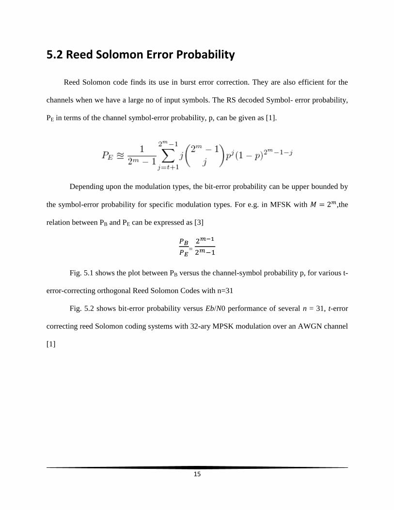
Reed Solomon code finds its use in burst error correction. They are also efficient for the
channels when we have a large no of input symbols. The RS decoded Symbol- error probability,
PE in terms of the channel symbol-error probability, p, can be given as [1].
Depending upon the modulation types, the bit-error probability can be upper bounded by
the symbol-error probability for specific modulation types. For e.g. in MFSK with ,the
relation between PB and PE can be expressed as [3]
=
Fig. 5.1 shows the plot between PB versus the channel-symbol probability p, for various t-
error-correcting orthogonal Reed Solomon Codes with n=31
Fig. 5.2 shows bit-error probability versus Eb/N0 performance of several n = 31, t-error
correcting reed Solomon coding systems with 32-ary MPSK modulation over an AWGN channel
[1]

16
Fig. 5.1 PB versus the channel-symbol probability p

17
Fig. 5.2 bit-error probability versus Eb/N0

18
5.3 RS Encoder
The generating polynomial for most conventional RS code (n, k) takes the form
g(X) = g0 +g1X + g2 ……+ g2t-1 +
Since the degree of generating polynomial is 2t, so there are 2t roots of generating
polynomial, which are the successive powers of α.Hence the roots of generating polynomial can
be designated as .we can start the root with any desired power of α.For example
consider RS code (7,3).The no parity bits in the code is n-k=4.Hence we can describe the
generating polynomial in terms of successive four power of α.
g(X)=
=
Consider the case for binary field +1= -1, g(X) can be expressed as
g(X ) = α3 + α
1 X + α
0 X
2 + α
3 X
3 + X
4
After that we calculate the parity polynomial as

19
The encoded symbol can be now written as,
5.4 RS Decoder
The received code word can be represented as a sum of encoded symbol and error symbol as
The most important sted in RS decoder is Syndrome Calculation. Since the encoded symbol can
be written as
Hence, the roots of generating polynomial also satisfy the roots of received polynomial if
the symbols are not in error. A non-zero value of syndrome indicates that resultant code word is
in error. After finding out non- zero syndrome. We calculate the error location and error values
using Reed-Solomon decoding algorithm.
An error-locator polynomial, σ(X ) , can be defined as follows:
The reciprocal of the roots of σ(X ) are the error-location numbers of the error pattern e(X ).
Then, using autoregressive modelling techniques, we form a matrix from the syndromes, where
the first t syndromes are used to predict the next syndrome. For the (7, 3) double-symbol error
correcting R-S code, the matrix size is 2 × 2, and the model is written as follows:

20
By solving above equations, we find out the error locations and error values.
5.5 MATLAB Simulation of (7, 3) RS Code
We wrote a program for (7,3) RS encoder and Decoder. We gave the data of 100 bits
generated randomly by the program itself. We encoded the whole message signal by the encoder
program. Then we introduced some random errors generated arbitrarily in the encoded signal.
After that, using the decoder program we decoded it and plotted the graph between the
percentage of the error introduced in the encoded signal and percentage of error in the final
decoded signal. The graph is shown in fig.
As seen from the graph the percentage of error after the decoded signal remains within
the limit when the percentage of error in the channel is up to 30 percent. After that the error in
the decoded signal increases with the increase in the percentage error.
This can be clearly understood from the theoretical calculations since we are able to detect
only two errors through (7,3) symbols. Hence up to 28 percent we are able to detect efficiently as
possible and after that there is no guarantee on how much is the percentage of error correction.

21
Fig. 5.3 MATLAB simulation of RS (7,3) code

22
Chapter 6
GF implementation for RS (255,239)
code in VHDL
6.1 Introduction
Here onwards we discuss the VHDL implementation of RS(255,239) code. In
RS(255,239) code, 255 is the total number of data symbols in a code word including parity
symbols, 239 is the number of data symbols excluding parity symbols, 16(255-239=16) are the
parity symbols added to the data symbols by the encoding process. Each symbols contain 8 bits
(so m=8) and error correcting capability of the code is 8 symbols (so t=8). That is why, we have
to add 16 (2*t=16) parity symbols.
To implement any RS code, first of all we have to choose and construct a particular field.
As explained in chapter 4, a field is always built using a primitive polynomial. For the
implementation of RS (255,239) code, a primitive polynomial of degree 8 has been chosen. As
we already know, galois field elements do not obey general binary operation like addition or
multiplication. Addition and Subtraction are performed by simple logical XOR operation, but we
need to design galois field multiplier and divider. However divider is implemented using inverse
element and multiplication techniques. Each design is described in this chapter one by one.
6.2 GF Multiplier
Multiplication in galois field is not as trivial as the addition and subtraction. Even
multiplication in a particular field is not applicable to another field with different primitive

23
polynomial. GF multiplier is the most used block in the design of encoder and decoder. Hence
implementation of the multiplier is the back bone of the design. In Our design GF(28) is used and
the primitive polynomial chosen is . The binary representation of this
primitive polynomial is 100011101.
The basic difference between binary multiplication and galois field multiplication is that
galois field is finite. So the result of the multiplication of two 8 bit galois field elements should
be of 8 bits but in case of binary multiplication it is of 16 bits. There are various approaches to
implement GF multiplier. These are discussed below.
Look up table approach: This approach is very simple to understand and to
implement also. The results of the multiplication of all the combination of
elements are stored in a lookup table. A particular address is used to access each
combination result from the look up table. This approach is useful for small fields.
For larger fields, the required memory size increases as the combination
increases.
Log-antilog approach: This approach simply uses the log antilog technique of the
multiplication of two numbers. The elements are mapped in terms of their power
and stored in a log table. After that these powers are added and the result are
found from the antilog table. This approach is however more efficient in terms of
resource utilisation but it still requires large memory for large fields like GF(28).
Logic implementation approach: In this approach, logic implementation is done
for the GF multiplier. This logic implementation may be either sequential or
combinational.

24
Sequential approach is similar to binary multiplication. Each bit of multiplier is
multiplied by the multiplicand. And the partial results are shifted and added to find out the result.
In addition additional effort is required as result should not exceed m bit. In the intermediate
stages of multiplication whenever a '1' is carried out of the 8 bit an additional XOR operation is
done. This XOR operation is derived from the primitive polynomial. Problem with this approach
is that it takes m clock cycles for multiplication in m bit Galois field. To work synchronously
with other operations it should run with a clock 8 times faster than the clock used for other
components.
In Combinational approach AND and XOR gates are used to generate the result. Logic
can be found out using classical truth table method. But this method is not suitable for large field
as the combinations become larger. Alternately logic can be derived using the general
multiplication steps and primitive polynomial. The delay introduced by combinational logic is
almost fixed. If the clock time period is higher than this delay then it can be used in a sequential
circuit without introducing further delay.
We have used combinational approach in our design. Logic is developed by simple
multiplication steps and primitive polynomial. This has been shown in table 6.1 [2]. The final
logic developed from the table has been found and reduced to as below [2].
Result (7) = A7B0 + A6B1 + A5B2 + A4B3 + A3B4 + A7B4 + A2B5 + A6B5 +A7B5 +A1B6 + A5B6 + A6B6 + A7B6 +
A0B7 + A4B7 + A5B7 + A6B7
Result (6) = A6B0 + A5B1 + A4B2 + A3B3 + A7B3 + A2B4 + A6B4 +A7B4 + A1B5+A5B5 + A6B5 + A7B5 + A0B6 +
A4B6 + A5B6 + A6B6 + A3B7 +A4B7 + A5B7
Result (5) = A5B0 + A4B1 + A3B2 + A7B2 + A2B3 + A6B3 + A7B3 +A1B4 + A5B4+A6B4 + A7B4 + A0B5 + A4B5 +
A5B5 + A6B5 + A3B6 + A4B6 +A5B6 + A2B7+A3B7 + A4B7
Result (4) = A4B0 + A3B1 + A7B1 + A2B2 + A6B2 + A7B2 + A1B3 +A5B3 + A6B3+A7B3 + A0B4 + A4B4 + A5B4 +
A6B4 + A3B5 + A4B5 + A5B5 +A2B6 + A3B6+A4B6 + A1B7 + A2B7 + A3B7 + A7B7

25
Table 6.1 GF Multiplier Table

26
Result (3) = A3B0 + A2B1 + A7B1 + A1B2 + A6B2 + A7B2 + A0B3 +A5B3 + A6B3+A4B4 + A5B4 + A7B4 + A3B5
+A4B5 + A6B5 + A7B5 + A2B6 +A3B6 + A5B6+A6B6 + A1B7 + A2B7 + A4B7 + A5B7
Result (2) = A2B0 + A1B1 + A7B1 + A0B2 + A6B2 + A5B3 + A7B3 +A4B4 + A6B4+A3B5 + A5B5 + A7B5 + A2B6 +
A4B6 + A6B6 + A7B6 + A1B7 +A3B7 + A5B7+A6B7
Result (1) = A1B0 + A0B1 + A7B2 + A6B3 + A5B4 + A4B5 + A3B6 +A7B6 + A2B7+A6B7 + A7B7
Result (0) = A0B0 + A7B1 + A6B2 + A5B3 + A4B4 + A3B5 + A7B5 +A2B6 + A6B6+A7B6 + A1B7 + A5B7 + A6B7 +
A7B7
It was implemented as a block and this block was used in the design of encoder and
decoder as a component. The block Diagram and the behavioural simulation of the GF multiplier
are shown in fig. 6.1 and 6.2 respectively.
Fig. 6.1 GF multiplier
Fig 6.2 Behavioural simulation of GF multiplier

27
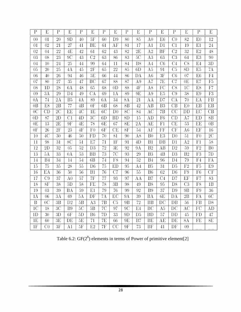
6.3 GF elements
All the elements of the field GF(28) is found by raising the power of primitive polynomial
in increasing order. The basic element is “00000001” that denotes α0 which is also called
primitive element. The generated field elements have been used in our design. Generated GF
elements against corresponding power of the primitive element expressed in hexadecimal form
have been given in table 6.2 [2].
6.4 Generator Polynomial
Generator Polynomial is the vital part of the RS encoder and decoder design. The
generator polynomial is used for the calculation of redundant symbols in RS encoder. It is also
used for detection of error in the decoder. The degree of the primitive polynomial is equal to the
number of the redundant symbols in the code word. So in our design, the order is 16. As
explained earlier, first 16 elements of the field are taken as the roots of the generator polynomial.
The coefficients of the generator polynomial in hexadecimal form are
01, 3B, 0D, 68, BD, 44, D1, 1E, 08, A3, 41, 29, E5, 62, 32, 24, 3B.
6.5 GF element inversion block
This block is used to find the inverse of the element. It is used in the implementation of
the GF divider. A lookup table has been used to store the element and its inverse. The addressing
is done corresponding to the powers of the primitive element. This block is used further in the
design of decoder as a building block.
28
Table 6.2: GF(28) elements in terms of Power of primitive element[2]

29
Chapter 7
RS Encoder Design
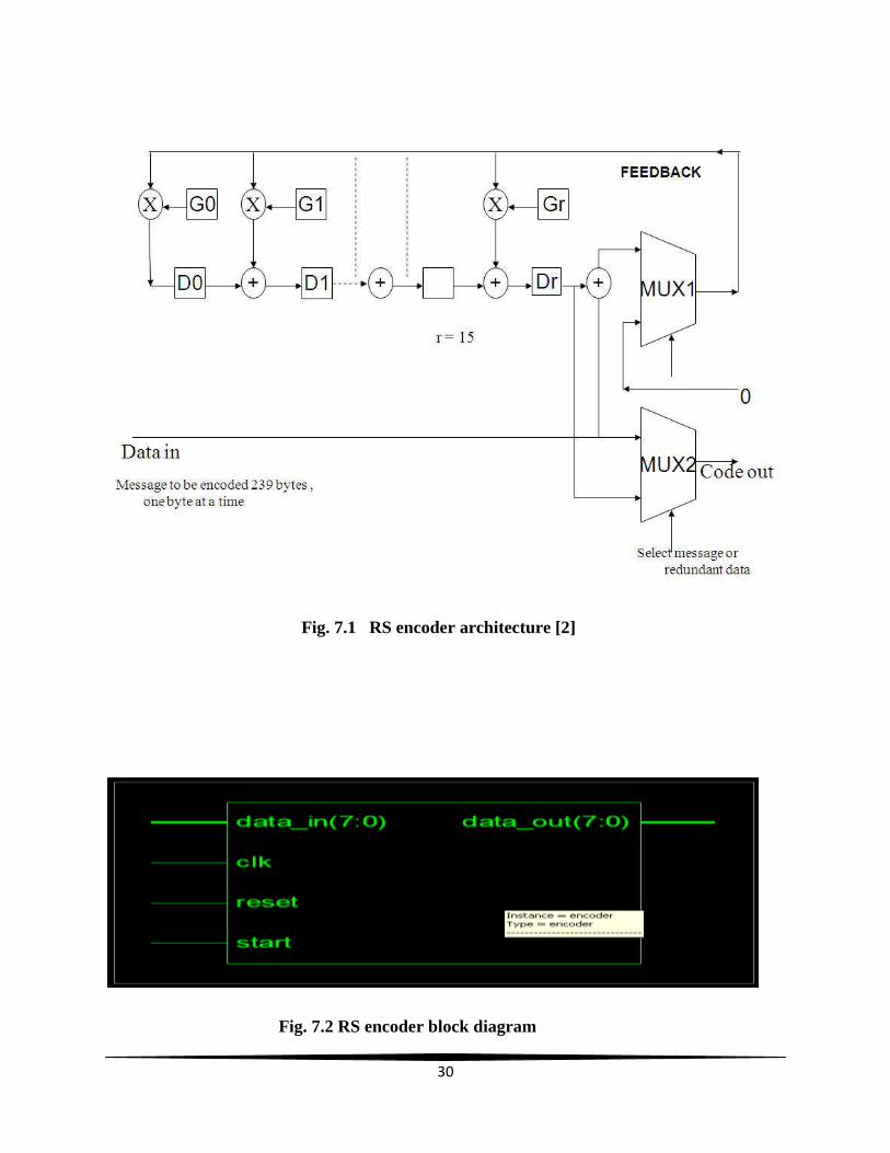
7.1 General Description
Though, RS encoding principle has been described in chapter 5. In this section, we
discuss the design of the encoder for RS(255,239) code in VHDL. The encoder has a generator
polynomial register, a shift register, two 2:1 multiplexers, 16 GF multipliers and 16 GF adders.
This has been shown in fig 7.1.
Generator polynomial has been stored in generator polynomial register. The shift register
has been initialized to all zeros. Data input is sent to the encoder one symbol at a time. As soon
as data to be encoded appears on the input, the select input of MUX1 is set such that the MUX1
selects the GF addition of input symbol and the highest degree coefficient of the shift register
polynomial which has been set to zero initially. The output of this MUX now becomes the
feedback. This feedback is multiplied with generator polynomial register contents which are the
generator polynomial coefficients. The result is added to the shift register polynomial and shifted
towards right once to update the shift register polynomial. MUX2 selects input data symbols to
pass to the encoder output. All these operation are synchronous. After 239 such clock cycles shift
register polynomial contains the redundant symbols. Now MUX2 selects other input and allow
the redundant symbols to pass to the encoder output.
30
Fig. 7.1 RS encoder architecture [2]
Fig. 7.2 RS encoder block diagram

31
8.2 Design details
The encoder has been designed as per the architecture described above. The encoder
block with its inputs and outputs is shown in fig 7.2. Input output description is given in table
7.1.
Signal Type Width Description
clk IN 1 Input clock signal
data_in IN 8 Input data symbols
data_out OUT 8 Encoded data symbols
reset IN 1 Active low reset signal
start IN 1 Active low signal used for the initiation
of encoding.
Table 7.1 Input output description of encoder
The encoder architecture is divided in two parts. First part consists of 16 GF multipliers,
16 GF adders and 16 shift registers. This part computes the redundant symbols from the input
data. Second part consists of two multiplexers which control the encoder output to be either input
symbols or redundant symbols which depends on the count of clock cycles. We implemented it
in VHDL and got a top level block diagram which is in two parts in shown in fig.7.3 and 7.4.
The behavioural simulation of the encoder is shown in fig. 7.5.

32
Fig. 7.3 RTL schematic of the encoder 1st part containing 16 redundant symbols generator
Fig. 7.4 RTL schematic of the encoder 2nd
part containing multiplexers
Fig.7.5 Behavioural simulation of the encoder showing only first few clock cycles
33
Chapter 8
RS Decoder Design
8.1 Introduction
The decoder principle has been described in chapter 5. In this chapter, we have explained
the details of decoder design implementation. Actually, decoding involves solving of equations
to find out the unknowns. These unknowns are the error locations and error values. For detecting
t errors, t error locations and t error magnitudes have been needed. Hence 2t equations have been
solved. This operation requires several steps to follow and in each step, there are several
algorithms to approach the problem. These are described as below.
Syndrome generation: Syndrome generation is the error detection stage. Syndrome has
been generated by evaluating the received polynomial at all the roots of the generator
polynomial. A nonzero syndrome has been an indication of error. Syndrome polynomial
has been used further for finding out the error location and magnitude.
Error location: Error location is found out by generating an error locator polynomial and
then solving it. Finding the error locator polynomial has been the most critical part of
decoding.
Error evaluation: Error evaluation has been done by generating an error evaluation
polynomial and solving it.

34
Error Correction: Error correction has been the last step in decoding. Correction has been
done by subtracting the error magnitude from the received data corresponding to each
error location.
RS decoder has been developed by designing several blocks using GF multipliers, adders,
counters, shift registers and GF inversion circuits, corresponding to each step and then
connecting those blocks. The decoder bock is shown in fig. 8.1. The input output description is
shown in table 8.1.
Fig. 8.1 RS decoder block
Signal Type Width Description
clk IN 1 Input clock signal
data_in IN 8 Received data symbols
data_out OUT 8 Decoded data symbols
reset IN 1 Active low reset signal
start IN 1 Active low signal used for the initiation
of decoding.
Table 8.1 Input output description of decoder

35
8.2 Design details
RS decoder has been designed following the steps explained above. Decoder has been
designed using modular approach. Different modules have been described here. Functional block
diagram has been shown in fig. 8.2.
Fig. 8.2 Functional block diagram of decoder
Syndrome Generator:
Syndrome generator has been the first module of the decoder which indicates whether the
received data is in error or not. Received data has been fed as input to syndrome generator.
Output has been produced in the form of a 16 degree polynomial. Mathematically the received
polynomial has been evaluated at all the roots of the generator polynomial used for encoding.
Here received polynomial is referred to received-codeword which has been 239 message
symbols followed by 16 redundant symbols. The symbols have been received starting from the
highest power. Each received codeword has been considered as one polynomial of degree 255.

36
Generator polynomial being of degree 16 has 16 roots. This operation is done using GF
multiplier and adders. The block diagram has been shown in figure 8.3. This operation has been
done with all the 16 roots taken as input. All the corresponding outputs have been coefficients of
the syndrome polynomial. Hence if all the roots of the generator polynomial satisfy the received
polynomial then syndrome has been found to be 0. This has been an indication of received
polynomial being a true codeword. A nonzero syndrome is the indication of the error and this
syndrome polynomial has been used to find the error locator polynomial. It takes 255 clock
cycles.
Error locator polynomial generator:
For finding the error locations a polynomial is formed whose roots are the reciprocal of the
error locations. This principle has been described in chapter 5. For large codes like RS (255,239)
the matrix method is quite complex. So, several algorithms are there to implement it. Some
important algorithms are Berlekamp's algorithm, Euclidian Algorithm, Binary GCD algorithm.
We have used binary GCD algorithm in our design. Binary GCD algorithm is explained
below.
Binary GCD algorithm [3]:
Let a(x) be a polynomial over the finite field GF (2m
):
ai
and its associated vector representation is denoted by a=[an-1; . . . a1, a0]. We can use the
following observations:
– If a(x) and b(x) are both „even‟, gcd(a, b)= x*gcd(a/x, b/x).

37
Fig.8.3 RS syndrome generator [2]

38
– If a(x) is „even‟ and b(x) is „odd‟, gcd(a, b)= gcd(a/x, b).
– Otherwise both are „odd‟, and gcd(a, b)-gcd([a+(a0/b0)b]= (x, b)
By the use of terminology, we say that a polynomial a(x) is „even‟ when a0=0 and „odd‟
otherwise. Now algorithm is
This polynomial has been used for locating the error. It has also been used for generation of the
error evaluator polynomial.
Error evaluator polynomial generator:
Error evaluator polynomial has been designed using error locator polynomial and syndrome
values. The following equation is used to find the error evaluator polynomial.
E(x) = S(x)*L(x)
Where E(x) is error evaluator polynomial of degree 8, S(x) is syndrome polynomial of degree 16
and L(x) is error locator polynomial of degree 8. The coefficients of this polynomial have been

39
calculated by GF multiplication and addition of the coefficients of syndrome polynomial and
error locator polynomial.
E(0)=S(0)*L(0);
E(1)= S(1)*L(0) + S(0)*L(1);
E(2)= S(2)*E(0) + S(1)*E(1) + S(0)*E(2);
...................................................................
..................................................................................
Only 8 lowest degree syndrome values are used because the degree of the error evaluator
polynomial is 8. The implementation is shown in fig. 8.4
Fig. 8.4 A part of RTL schematic of error evaluator polynomial generator
Error locator:
In error locator, error locator polynomial is used to find the error locations. Basically errors
locations are the inverse of the roots of the error locator polynomial. To find the roots, we

40
evaluate the error locator polynomial at every element of the field. When this value is zero, that
element is the root of the polynomial. Now there are two approaches to implement it. First
approach is to use 255 GF multipliers and adders. It takes lots of space on the FPGA but has low
latency. Second approach uses only 8 GF multipliers and adders. It takes less area on FPGA but
takes 255 cycles to compute error locations i.e. it has high latency. Once, the roots are found out,
their inverse is taken to find the error locations. Inversion is performed by element inversion
block discussed in chapter 6.
Error evaluator:
After the error locations have been found, the next operation is to compute error values. Error
values are computed by Forney algorithm. According to Forney algorithm, the error value at
error location x is given by
The inverse of the error location is taken and error evaluator and error locator polynomial are
computed at that inverted root to find the error magnitude by the above formula. The division is
performed by inverting the denominator value by inversion block. A snapshot of the RTL
schematic of the error evaluator is shown in fig. 8.5.

41
Fig. 8.5 A part of the RTL schematic of error evaluator
Data Correction:
After the error and its location have been evaluated, the received data has to be corrected for
these errors. The correction is simply the subtraction of the errors from the received data. In
galois field the subtraction and the addition are nothing but the XOR of the two operands. So the
errors are XORed with the individual symbol of the received data. The implementation simply
uses the error values and the accumulate logic to get the correct data. But the delay introduced in
the path of the error computation plays a major role in this. All the symbols should be delayed by
a fixed time which would be equal to error evaluation time for that symbol. Both the received
symbol and corresponding error should reach at error corrector at the same time. And correct
symbol at that location should be calculated and sent.

42
Chapter 9
Results and Conclusion
9.1 Results
Though, the RTL schematic and also the behavioural simulation of the blocks have been
shown with their design details in the previous chapters. Here we show the details regarding the
FPGA utilisation and timing of the operation for the encoder and decoder separately.
RS Encoder:-
CLBs used = 156,
clock cycles needed = 255
RS Decoder:-
clock cycles needed = 255+16+1+8+8+8
= 255+41
= 296
In RS encoder, one clock cycle is needed for every data symbol and hence total of 255
clock cycles are needed for one code word. In RS decoder, 255 clock cycles are needed only for
the syndrome computation, next 16 clock cycles are needed for evaluating the coefficient of error
locator polynomial. Only one clock cycle is needed for the computation of coefficients of the
error evaluator polynomial. 8 clock cycles are needed to compute the error locations from error
locator polynomial. 8 clock cycles are needed to compute the error values from error evaluator

43
polynomial. Now finally, 8 clock cycles are needed to correct the data symbols. So total of 296
clock cycles are needed in decoder.
9.2 Conclusion and future work
To have an efficient and reliable communication system, the error correction techniques
have to be improved over the years. Various forward error correction techniques have been
studied and compared. Among all the FECs, Reed Solomon code has been found to be the most
suitable code because of the low coding complexity and high coding rate etc. Specifically, RS
code is the most efficient in the case of bust error correction. It provides excellent error
correcting abilities since this is a non binary symbolic code.
The RS encoder and decoder were designed in the most efficient algorithms to optimise
the FPGA utilisation and latency of the code. These two factors have to be optimised at the cost
of each other. That is why, we analysed various algorithms for these factors and implemented in
most suitable algorithms in order to optimise the design. The encoder and decoder which has
been designed, can be used for both transmission and storage of the data.
The field of communication is highly growing area in research. The goal is to reduce the
space and increase the efficiency. The development of highly effective algorithms for the
implementation is the area where the significant amount of research work can be done and RS
code can be made more suitable in highly reactive system where the data transfer rate is very
fast.

44
Bibliography
[1] Reed-Solomon Codes by Bernard Sklar (http://ptgmedia.pearsoncmg.com/images/art_sklar7_reed-solomon/elementLinks/art_sklar7_reed-
solomon.pdf)
[2] Ashutosh Mohanty, “Implementation of Reed Solomon Error
Correction Code” NIT Rourkela, Aug 2009.
[3] F. Arguello : “Binary GCD algorithm for computing error locator
polynomials in Reed-Solomon decoding” ELECTRONICS LETTERS
23rd June 2005 Vol. 41 No. 13.
[4] BOOK: Taub and Schilling, “Principle of Communication Systems”
[5] Reed, I. S. and Solomon, G., “Polynomial Codes Over Certain Finite
Fields,” SIAM Journal of Applied Math., vol. 8, 1960, pp. 300-304.
[6] Gallager, R. G., Information Theory and Reliable Communication
(New York: John Wiley and Sons, 1968).
[7] Proakis John G., Salehi M., _Communication System Engineering_,
Second Edition, Prentice Hall of India, 2005
[8] James S. Plank “A Tutorial on Reed-Solomon Coding for Fault-
Tolerance in RAID like Systems” Technical Report CS-96-332,
Department of Computer Science, University of Tennessee
[9] Zhigang Ren, Dongping Yao “An Improved High-speed RS
Encoding Algorithm” College of Electronic Information Engineering
Beijing, Jiaotong University, Beijing, China
45
[10] Stephen B. Wicker “An Introduction to Reed-Solomon Codes
“School of Electrical and Computer Engineering, Georgia Institute of
Technology Atlanta, Georgia 30332
[11] http://en.wikipedia.org/wiki [12] http://www.eccpage.com/
[13] http://www.google.com
Top Related