Visualized Insights into the Optimization Landscape ofFully Convolutional Networks

Jianjie Lu,1 Kai-yu Tong2

The Chinese University of Hong Kong1 Department of Electronic Engineering, jacklu@link.cuhk.edu.hk2 Department of Biomedical Engineering, kytong@cuhk.edu.hk

Shatin, NT, Hong Kong SAR, China, 999077

Abstract

Many image processing tasks involve image-to-image map-ping, which can be addressed well by fully convolutionalnetworks (FCN) without any heavy preprocessing. Althoughempirically designing and training FCNs can achieve satis-factory results, reasons for the improvement in performanceare slightly ambiguous. Our study is to make progress in un-derstanding their generalization abilities through visualizingthe optimization landscapes. The visualization of objectivefunctions is obtained by choosing a solution and projectingits vicinity onto a 3D space. We compare three FCN-basednetworks (two existing models and a new proposed in thispaper for comparison) on multiple datasets. It has been ob-served in practice that the connections from the pre-pooledfeature maps to the post-upsampled can achieve better results.We investigate the cause and provide experiments to showsthat the skip-layer connections in FCN can promote flat opti-mization landscape, which is well known to generalize better.Additionally, we explore the relationship between the modelsgeneralization ability and loss surface under different batchsizes. Results show that large-batch training makes the modelconverge to sharp minimizers with chaotic vicinities whilesmall-batch method leads the model to flat minimizers withsmooth and nearly convex regions. Our work may contributeto insights and analysis for designing and training FCNs.

IntroductionIt is generally difficult to solve some image processingproblems without complicated procedures. For instance, innatural image edge detection, using edge detectors suchas Canny operator is unable to obtain satisfactory results(Ganin and Lempitsky 2014). The textures may be ex-tremely complex while in some cases we expect models tooutput specific edges instead of all in the whole image.

In fact, many of these problems can be treated as map-ping an input image to a corresponding output image. Differ-ent fully convolutional networks (FCN) have achieved greatsuccess in image-to-image tasks and enable them to be tack-led end-to-end. The concept of FCN is first introduced forpixel-to-pixel semantic segmentation by removing fully con-nected layers and inserting upsampling layers at the end ofnetworks (Long, Shelhamer and Darrell 2015).

Copyright c© 2019, Association for the Advancement of ArtificialIntelligence (www.aaai.org). All rights reserved.

With this approach, many classification networks can beconverted for image-to-image mapping (Xie and Tu 2015;Liu et al. 2017). They use upsampling layers to recover fromfeature maps with different resolutions and a fusion layerto output the final image. These models show good perfor-mance in edge detection of natural images. Apart from mod-ifying classification networks, (Ronneberger, Fischer andBrox 2015) design an encoder-decoder structure consist-ing of a contracting path and multiple expanding paths tocapture context at different scales. It has been applied forbiomedical image segmentation successfully.

Trying and training different architectures empirically canobtain satisfactory results but clear understandings of the im-provement in performance are insufficient. Theoretically ex-ploring loss surfaces of classification neural networks havebeen proposed recently (Nguyen and Hein 2018; Liang etal. 2018). (Li et al. 2017) shows that the residual mappingstructure can lead to a convex objective function using a vi-sualization method. However, there is no similar analysis onFCNs, which have totally different structures and objectivefunctions from classification models. Therefore, we make anexploration on FCN-based networks by choosing a solutionand projecting its vicinity along two random vectors. To thebest of our knowledge, our paper is the first to provide a vi-sualized insight into the minimizers geometry of FCNs andtheir generalization abilities.

The rest of this paper is organized as follows. Firstly, rep-resentative FCN-based models and visualization approachesare discussed. Then we introduce the objective function, vi-sualization method as well as different architectures used forcomparison in this study. Thirdly, we evaluate these FCNson multiple datasets and visualize the optimization land-scapes to understand their generalization abilities. Detailedanalysis is also provided. Finally, we conclude the paper.

Related WorkFull Convolutional NetworksFully convolutional network (FCN) is first proposed in(Long, Shelhamer and Darrell 2015), which makes it possi-ble for image classification networks to output segmentationresults. In general, fully connected layers are applied at theend of CNN to predict class scores. Features maps will beflattened and fed into classifier layers. Space information is

arX

iv:1

901.

0855

6v1

[cs

.LG

] 2

0 Ja

n 20

19

lost due to this squeezing operation. They replace the fullyconnected layers with upsampling or de-convolution layers.Therefore, image classification models can operate inputs ofany size and generate corresponding output images.

Many basic classification networks, such as VGG-Net(Simonyan and Zisserman 2015), can be used as a back-bone for learning image mapping by leveraging techniquesin (Long, Shelhamer and Darrell 2015). Holistically-nestedEdge Detector (HED) extracts features with different reso-lutions from five layers of VGG-Net and upsamples them tooriginal scales (Xie and Tu 2015). At the end of the model,it uses a fusion layer to concatenate the features maps ina given dimension and output a corresponding result. Be-sides both SegNet and DeconvNet have a structure consist-ing of an encoder network and a decoder network, wherethe encoder topology is identical to VGG-Net (Noh, Hongand Han. 2015; Vijay, Alex and Roberto 2017). These twomodels learn to do upsampling using transposed convolutionand then convolve with kernels to produce feature maps forsegmentation.

Instead of modifying classification models, another typeof networks consist of a contracting path to capture contextand multiple symmetric expanding paths that enable preciselocalization. U-Net is one of the most representative models,which is initially designed for biomedical image segmenta-tion and won the ISBI cell tracking challenge in 2015 bya large margin (Ronneberger, Fischer and Brox 2015). Fur-ther variations of U-Net are proposed to solve different tasksin the literature (Milletari, Navab and Ahmadi 2016; Litjenset al. 2017). (Santhanam, Morariu and Davis 2017) createsa similar framework and achieves good performance on re-lighting, denoising and colorization.

Unlike the former methods, (Zhang et al. 2017) designsan FCN that removes all pooling layers and keeps the im-age size inside for image denoising. Batch normalizationand residual learning are also integrated to boost the trainingprocess as well as the performance. They achieve decent de-noising results, though this architecture may have relativelysmaller receptive field and higher computing resources con-sumption.

Visualization Methods

Although a large number of FCNs have been designed forvarious tasks, visualized methods are only applied on clas-sification networks. It is well known that the objective func-tion of deep neural networks lies in a super high dimensionalspace. As a result, we can only visualize it in 2D or 3D space.

A widely-used 2D plotting method is linear interpolation,which is first applied to study local minimizers under differ-ent batch size settings (Dinh et al. 2017; Keskar et al. 2017).An alternate approach is projection. (Goodfellow, Vinyalsand Saxe 2015) uses this approach to explore the trajectoriesof different optimization algorithms. (Li et al. 2017) studiesthe relationship between loss landscapes and models gener-alization abilities by projection. Note that these studies onlyfocus on classification networks, whose structures and ob-jective functions are entirely different from FCNs.

MethodObjective FunctionImage-to-image mapping problems can be converted aspixel regression or classification using FCNs. The main dif-ference is whether the output is continuous or categorical.

We train networks as a regression problem since pixel-wise class labels are slightly difficult to obtain in practice.For instance, the raindrop removal dataset only providesoriginal images as labels. Therefore, we use mean square er-ror (MSE) as the objective function, which can be expressedas follows:

L =1

N

N∑i=1

M∑t=1

(yit − yit) (1)

where N is used to represent the number of samples and Mdenotes the dimension of outputs. Generally, the L1 loss andMSE loss are almost the same in terms of regression accu-racy, while sometimes the result of MSE is slightly better(Zhang et al. 2016).

Visualization of Optimization LandscapesBy following (Goodfellow, Vinyals and Saxe 2015; Li etal. 2017), we choose a solution θ

′of the network with pa-

rameters θ and sample two set of random vectors u ={u1, u2, , u|θ|}and v = {v1, v2, , v|θ|} from a Gaussian dis-tribution N(µ,Σ), where |θ| denotes the number of filters inFCNs, µ is set at zero and Σ is assumed to be the identitymatrix I . After that, the optimization landscape can be plot-ted by projecting the vicinity of θ

′onto a 3D space along

these two random directions. It can be formulated as the fol-lowing equation:

f(α, β) = L(θ′+ α

u

‖u‖+ β

v

‖v‖) (2)

where α and β determine the optimization step size. Wedo filter-wise normalization by dividing the L2 norm ofeach sampled vector ui and vi. For better understanding ourmethod, the pseudocode of visualization algorithm is pro-vided in Algorithm 1.

There may be two ambiguities about this approach. Oneis probably about the generalization of local minimizers. Al-though finding a global minimum turns out to be an NP-hardproblem for the non-convex objective function of deep neu-ral networks, (Kawaguchi 2016; Lu and Kawaguchi 2017)show that local minima is not an issue for networks to gen-eralize well. Another consideration may be the repeatabil-ity of 3D projection plot using random vectors for the high-dimension loss functions. (Li et al. 2017) has shown thatdifferent random directions can produce similar shape byplotting multiple times. This phenomenon also exists in ourexperiments.

Fully Convolutional NetworksWe compare three fully convolutional networks includingtwo existing representative models (FCN-16s, U-Net) and anew proposed. Figure 1 shows the brief illustrations of thesethree structures.

Algorithm 1 Visualize Loss Function L

Input: A solution θ′of the network, plotting resolution n

and a visualization interval [−r, r]Output: A n× n loss matrix F1: while i = 1, 2, , |θ| do2: sample ui from N(0, Ii), where Ii has the same di-

mension as i-th filter θi of the network3: sample vi from N(0, Ii)4: ui = ui

‖ui‖5: vi = vi

‖vi‖6: end while7: while t = 0, 1, , n do8: αt = −r + 2r tn9: while k = 0, 1, , n do

10: βk = −r + 2r kn11: θnew = ∅12: for i = 1, 2, , |θ| do13: θi = θ

′

i + αtui + βkvi14: θnew = θnew ∪ θi15: end for16: Ft,k = L(θnew)17: end while18: end while19: return F

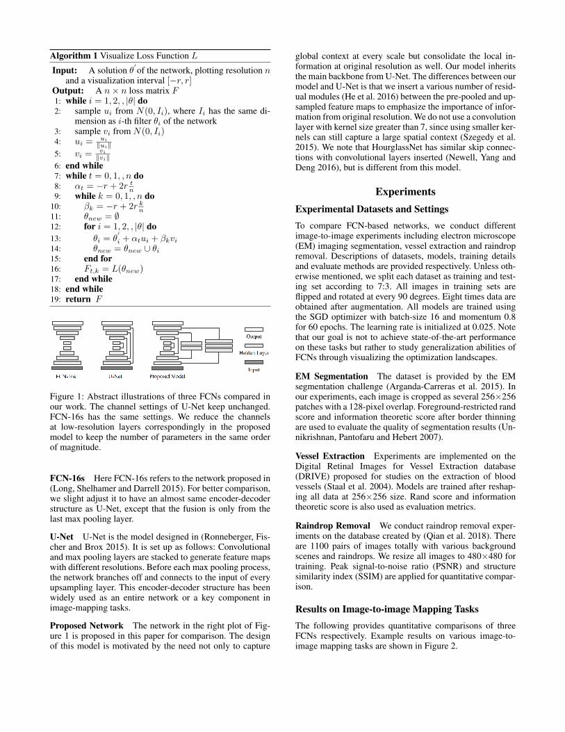
Figure 1: Abstract illustrations of three FCNs compared inour work. The channel settings of U-Net keep unchanged.FCN-16s has the same settings. We reduce the channelsat low-resolution layers correspondingly in the proposedmodel to keep the number of parameters in the same orderof magnitude.

FCN-16s Here FCN-16s refers to the network proposed in(Long, Shelhamer and Darrell 2015). For better comparison,we slight adjust it to have an almost same encoder-decoderstructure as U-Net, except that the fusion is only from thelast max pooling layer.

U-Net U-Net is the model designed in (Ronneberger, Fis-cher and Brox 2015). It is set up as follows: Convolutionaland max pooling layers are stacked to generate feature mapswith different resolutions. Before each max pooling process,the network branches off and connects to the input of everyupsampling layer. This encoder-decoder structure has beenwidely used as an entire network or a key component inimage-mapping tasks.

Proposed Network The network in the right plot of Fig-ure 1 is proposed in this paper for comparison. The designof this model is motivated by the need not only to capture

global context at every scale but consolidate the local in-formation at original resolution as well. Our model inheritsthe main backbone from U-Net. The differences between ourmodel and U-Net is that we insert a various number of resid-ual modules (He et al. 2016) between the pre-pooled and up-sampled feature maps to emphasize the importance of infor-mation from original resolution. We do not use a convolutionlayer with kernel size greater than 7, since using smaller ker-nels can still capture a large spatial context (Szegedy et al.2015). We note that HourglassNet has similar skip connec-tions with convolutional layers inserted (Newell, Yang andDeng 2016), but is different from this model.

ExperimentsExperimental Datasets and SettingsTo compare FCN-based networks, we conduct differentimage-to-image experiments including electron microscope(EM) imaging segmentation, vessel extraction and raindropremoval. Descriptions of datasets, models, training detailsand evaluate methods are provided respectively. Unless oth-erwise mentioned, we split each dataset as training and test-ing set according to 7:3. All images in training sets areflipped and rotated at every 90 degrees. Eight times data areobtained after augmentation. All models are trained usingthe SGD optimizer with batch-size 16 and momentum 0.8for 60 epochs. The learning rate is initialized at 0.025. Notethat our goal is not to achieve state-of-the-art performanceon these tasks but rather to study generalization abilities ofFCNs through visualizing the optimization landscapes.

EM Segmentation The dataset is provided by the EMsegmentation challenge (Arganda-Carreras et al. 2015). Inour experiments, each image is cropped as several 256×256patches with a 128-pixel overlap. Foreground-restricted randscore and information theoretic score after border thinningare used to evaluate the quality of segmentation results (Un-nikrishnan, Pantofaru and Hebert 2007).

Vessel Extraction Experiments are implemented on theDigital Retinal Images for Vessel Extraction database(DRIVE) proposed for studies on the extraction of bloodvessels (Staal et al. 2004). Models are trained after reshap-ing all data at 256×256 size. Rand score and informationtheoretic score is also used as evaluation metrics.

Raindrop Removal We conduct raindrop removal exper-iments on the database created by (Qian et al. 2018). Thereare 1100 pairs of images totally with various backgroundscenes and raindrops. We resize all images to 480×480 fortraining. Peak signal-to-noise ratio (PSNR) and structuresimilarity index (SSIM) are applied for quantitative compar-ison.

Results on Image-to-image Mapping TasksThe following provides quantitative comparisons of threeFCNs respectively. Example results on various image-to-image mapping tasks are shown in Figure 2.

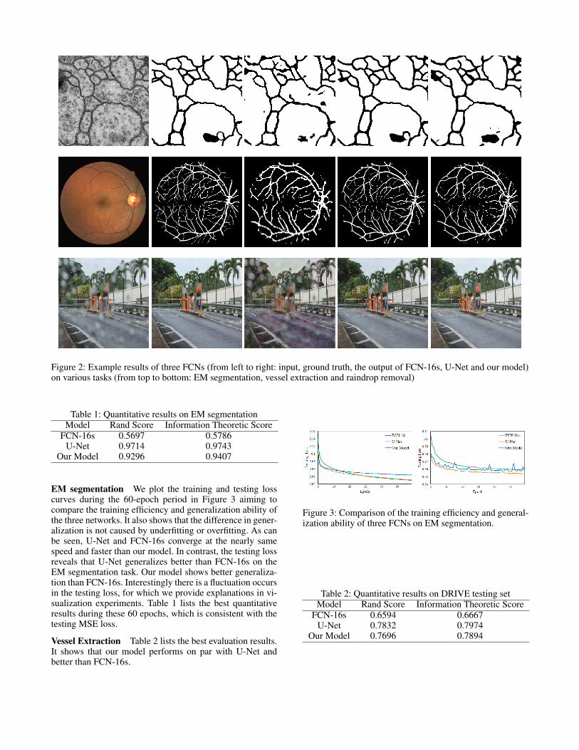
Figure 2: Example results of three FCNs (from left to right: input, ground truth, the output of FCN-16s, U-Net and our model)on various tasks (from top to bottom: EM segmentation, vessel extraction and raindrop removal)

Table 1: Quantitative results on EM segmentationModel Rand Score Information Theoretic Score

FCN-16s 0.5697 0.5786U-Net 0.9714 0.9743

Our Model 0.9296 0.9407

EM segmentation We plot the training and testing losscurves during the 60-epoch period in Figure 3 aiming tocompare the training efficiency and generalization ability ofthe three networks. It also shows that the difference in gener-alization is not caused by underfitting or overfitting. As canbe seen, U-Net and FCN-16s converge at the nearly samespeed and faster than our model. In contrast, the testing lossreveals that U-Net generalizes better than FCN-16s on theEM segmentation task. Our model shows better generaliza-tion than FCN-16s. Interestingly there is a fluctuation occursin the testing loss, for which we provide explanations in vi-sualization experiments. Table 1 lists the best quantitativeresults during these 60 epochs, which is consistent with thetesting MSE loss.

Vessel Extraction Table 2 lists the best evaluation results.It shows that our model performs on par with U-Net andbetter than FCN-16s.

Figure 3: Comparison of the training efficiency and general-ization ability of three FCNs on EM segmentation.

Table 2: Quantitative results on DRIVE testing setModel Rand Score Information Theoretic Score

FCN-16s 0.6594 0.6667U-Net 0.7832 0.7974

Our Model 0.7696 0.7894

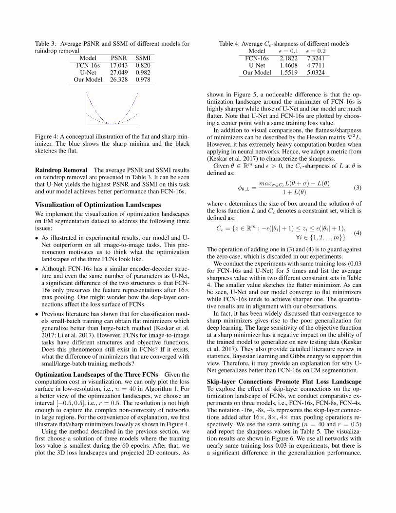
Table 3: Average PSNR and SSMI of different models forraindrop removal

Model PSNR SSMIFCN-16s 17.043 0.820

U-Net 27.049 0.982Our Model 26.328 0.978

Figure 4: A conceptual illustration of the flat and sharp min-imizer. The blue shows the sharp minima and the blacksketches the flat.

Raindrop Removal The average PSNR and SSMI resultson raindrop removal are presented in Table 3. It can be seenthat U-Net yields the highest PSNR and SSMI on this taskand our model achieves better performance than FCN-16s.

Visualization of Optimization LandscapesWe implement the visualization of optimization landscapeson EM segmentation dataset to address the following threeissues:• As illustrated in experimental results, our model and U-

Net outperform on all image-to-image tasks. This phe-nomenon motivates us to think what the optimizationlandscapes of the three FCNs look like.

• Although FCN-16s has a similar encoder-decoder struc-ture and even the same number of parameters as U-Net,a significant difference of the two structures is that FCN-16s only preserves the feature representations after 16×max pooling. One might wonder how the skip-layer con-nections affect the loss surface of FCNs.

• Previous literature has shown that for classification mod-els small-batch training can obtain flat minimizers whichgeneralize better than large-batch method (Keskar et al.2017; Li et al. 2017). However, FCNs for image-to-imagetasks have different structures and objective functions.Does this phenomenon still exist in FCNs? If it exists,what the difference of minimizers that are converged withsmall/large-batch training methods?

Optimization Landscapes of the Three FCNs Given thecomputation cost in visualization, we can only plot the losssurface in low-resolution, i.e., n = 40 in Algorithm 1. Fora better view of the optimization landscapes, we choose aninterval [−0.5, 0.5], i.e., r = 0.5. The resolution is not highenough to capture the complex non-convexity of networksin large regions. For the convenience of explanation, we firstillustrate flat/sharp minimizers loosely as shown in Figure 4.

Using the method described in the previous section, wefirst choose a solution of three models where the trainingloss value is smallest during the 60 epochs. After that, weplot the 3D loss landscapes and projected 2D contours. As

Table 4: Average Cε-sharpness of different modelsModel ε = 0.1 ε = 0.2

FCN-16s 2.1822 7.3241U-Net 1.4608 4.7711

Our Model 1.5519 5.0324

shown in Figure 5, a noticeable difference is that the op-timization landscape around the minimizer of FCN-16s ishighly sharper while those of U-Net and our model are muchflatter. Note that U-Net and FCN-16s are plotted by choos-ing a center point with a same training loss value.

In addition to visual comparisons, the flatness/sharpnessof minimizers can be described by the Hessian matrix∇2L.However, it has extremely heavy computation burden whenapplying in neural networks. Hence, we adopt a metric from(Keskar et al. 2017) to characterize the sharpness.

Given θ ∈ Rm and ε > 0, the Cε-sharpness of L at θ isdefined as:

φθ,L =maxσ∈CεL(θ + σ)− L(θ)

1 + L(θ)(3)

where ε determines the size of box around the solution θ ofthe loss function L and Cε denotes a constraint set, which isdefined as:

Cε = {z ∈ Rm : −ε(|θi|+ 1) ≤ zi ≤ ε(|θi|+ 1),

∀i ∈ {1, 2, ...,m}} (4)

The operation of adding one in (3) and (4) is to guard againstthe zero case, which is discarded in our experiments.

We conduct the experiments with same training loss (0.03for FCN-16s and U-Net) for 5 times and list the averagesharpness value within two different constraint sets in Table4. The smaller value sketches the flatter minimizer. As canbe seen, U-Net and our model converge to flat minimizerswhile FCN-16s tends to achieve sharper one. The quantita-tive results are in alignment with our observations.

In fact, it has been widely discussed that convergence tosharp minimizers gives rise to the poor generalization fordeep learning. The large sensitivity of the objective functionat a sharp minimizer has a negative impact on the ability ofthe trained model to generalize on new testing data (Keskaret al. 2017). They also provide detailed literature review instatistics, Bayesian learning and Gibbs energy to support thisview. Therefore, it may provide an explanation for why U-Net generalizes better than FCN-16s on EM segmentation.

Skip-layer Connections Promote Flat Loss LandscapeTo explore the effect of skip-layer connections on the op-timization landscape of FCNs, we conduct comparative ex-periments on three models, i.e., FCN-16s, FCN-8s, FCN-4s.The notation -16s, -8s, -4s represents the skip-layer connec-tions added after 16×, 8×, 4× max pooling operations re-spectively. We use the same setting (n = 40 and r = 0.5)and report the sharpness values in Table 5. The visualiza-tion results are shown in Figure 6. We use all networks withnearly same training loss 0.03 in experiments, but there isa significant difference in the generalization performance.

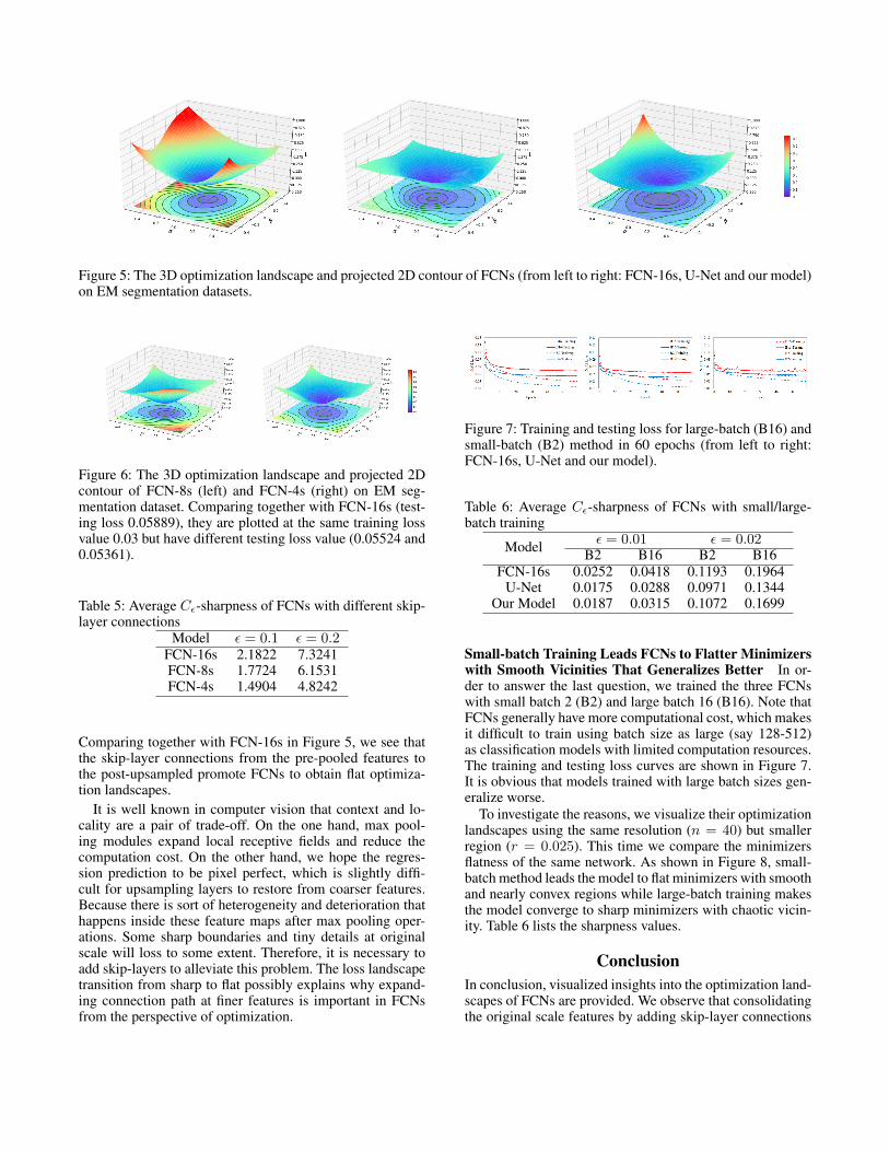
Figure 5: The 3D optimization landscape and projected 2D contour of FCNs (from left to right: FCN-16s, U-Net and our model)on EM segmentation datasets.

Figure 6: The 3D optimization landscape and projected 2Dcontour of FCN-8s (left) and FCN-4s (right) on EM seg-mentation dataset. Comparing together with FCN-16s (test-ing loss 0.05889), they are plotted at the same training lossvalue 0.03 but have different testing loss value (0.05524 and0.05361).

Table 5: Average Cε-sharpness of FCNs with different skip-layer connections

Model ε = 0.1 ε = 0.2FCN-16s 2.1822 7.3241FCN-8s 1.7724 6.1531FCN-4s 1.4904 4.8242

Comparing together with FCN-16s in Figure 5, we see thatthe skip-layer connections from the pre-pooled features tothe post-upsampled promote FCNs to obtain flat optimiza-tion landscapes.

It is well known in computer vision that context and lo-cality are a pair of trade-off. On the one hand, max pool-ing modules expand local receptive fields and reduce thecomputation cost. On the other hand, we hope the regres-sion prediction to be pixel perfect, which is slightly diffi-cult for upsampling layers to restore from coarser features.Because there is sort of heterogeneity and deterioration thathappens inside these feature maps after max pooling oper-ations. Some sharp boundaries and tiny details at originalscale will loss to some extent. Therefore, it is necessary toadd skip-layers to alleviate this problem. The loss landscapetransition from sharp to flat possibly explains why expand-ing connection path at finer features is important in FCNsfrom the perspective of optimization.

Figure 7: Training and testing loss for large-batch (B16) andsmall-batch (B2) method in 60 epochs (from left to right:FCN-16s, U-Net and our model).

Table 6: Average Cε-sharpness of FCNs with small/large-batch training

Model ε = 0.01 ε = 0.02B2 B16 B2 B16

FCN-16s 0.0252 0.0418 0.1193 0.1964U-Net 0.0175 0.0288 0.0971 0.1344

Our Model 0.0187 0.0315 0.1072 0.1699

Small-batch Training Leads FCNs to Flatter Minimizerswith Smooth Vicinities That Generalizes Better In or-der to answer the last question, we trained the three FCNswith small batch 2 (B2) and large batch 16 (B16). Note thatFCNs generally have more computational cost, which makesit difficult to train using batch size as large (say 128-512)as classification models with limited computation resources.The training and testing loss curves are shown in Figure 7.It is obvious that models trained with large batch sizes gen-eralize worse.

To investigate the reasons, we visualize their optimizationlandscapes using the same resolution (n = 40) but smallerregion (r = 0.025). This time we compare the minimizersflatness of the same network. As shown in Figure 8, small-batch method leads the model to flat minimizers with smoothand nearly convex regions while large-batch training makesthe model converge to sharp minimizers with chaotic vicin-ity. Table 6 lists the sharpness values.

ConclusionIn conclusion, visualized insights into the optimization land-scapes of FCNs are provided. We observe that consolidatingthe original scale features by adding skip-layer connections

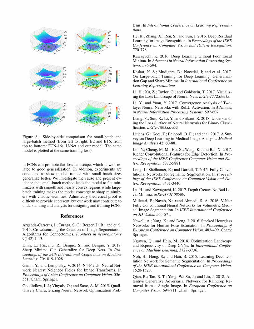
Figure 8: Side-by-side comparison for small-batch andlarge-batch method (from left to right: B2 and B16; fromtop to bottom: FCN-16s, U-Net and our model. The samemodel is plotted at the same training loss).

in FCNs can promote flat loss landscape, which is well re-lated to good generalization. In addition, experiments areconducted to show models trained with small batch sizesgeneralize better. We investigate the cause and present ev-idence that small-batch method leads the model to flat min-imizers with smooth and nearly convex regions while large-batch training makes the model converge to sharp minimiz-ers with chaotic vicinities. Admittedly theoretical proof isdifficult to provide at present, but our work may contribute tounderstanding and analysis for designing and training FCNs.

References

Arganda-Carreras, I.; Turaga, S. C.; Berger, D. R.; and et al.2015. Crowdsourcing the Creation of Image SegmentationAlgorithms for Connectomics. Frontiers in neuroanatomy9(142):1-13.

Dinh, L.; Pascanu, R.; Bengio, S.; and Bengio, Y. 2017.Sharp Minima Can Generalize for Deep Nets. In Pro-ceedings of the 34th International Conference on MachineLearning, 70:1019-1028.

Ganin, Y., and Lempitsky, V. 2014. N4-Fields: Neural Net-work Nearest Neighbor Fields for Image Transforms. InProceedings of Asian Conference on Computer Vision, 536-551. Cham: Springer.

Goodfellow, I. J.; Vinyals, O.; and Saxe, A. M. 2015. Quali-tatively Characterizing Neural Network Optimization Prob-

lems. In International Conference on Learning Representa-tions.

He, K.; Zhang, X.; Ren, S.; and Sun, J. 2016. Deep ResidualLearning for Image Recognition. In Proceedings of the IEEEConference on Computer Vision and Pattern Recognition,770-778.

Kawaguchi, K. 2016. Deep Learning without Poor LocalMinima. In Advances in Neural Information Processing Sys-tems, 586-594.

Keskar, N. S.; Mudigere, D.; Nocedal, J; and et al. 2017.On Large-batch Training for Deep Learning: Generaliza-tion Gap and Sharp Minima. In International Conference onLearning Representations.

Li, H.; Xu, Z.; Taylor, G.; and Goldstein, T. 2017. Visualiz-ing the Loss Landscape of Neural Nets. arXiv:1712.09913.

Li, Y.; and Yuan, Y. 2017. Convergence Analysis of Two-layer Neural Networks with ReLU Activation. In Advancesin Neural Information Processing Systems, 597-607.

Liang, S.; Sun, R.; Li, Y.; and Srikant, R. 2018. Understand-ing the Loss Surface of Neural Networks for Binary Classi-fication. arXiv:1803.00909.

Litjens, G.; Kooi, T.; Bejnordi, B. E.; and et al. 2017. A Sur-vey on Deep Learning in Medical Image Analysis. MedicalImage Analysis 42: 60-88.

Liu, Y.; Cheng, M. M.; Hu, X.; Wang, K.; and Bai, X. 2017.Richer Convolutional Features for Edge Detection. In Pro-ceedings of the IEEE Conference Computer Vision and Pat-tern Recognition, 5872-5881.

Long, J.; Shelhamer, E.; and Darrell, T. 2015. Fully Convo-lutional Networks for Semantic Segmentation. In Proceed-ings of the IEEE Conference on Computer Vision and Pat-tern Recognition, 3431-3440.

Lu, H.; and Kawaguchi, K. 2017. Depth Creates No Bad Lo-cal Minima. arXiv:1702.08580.

Milletari, F.; Navab, N.; xand Ahmadi, S. A. 2016. V-Net:Fully Convolutional Neural Networks for Volumetric Medi-cal Image Segmentation. In IEEE International Conferenceon 3D Vision, 565-571.

Newell, A.; Yang, K.; and Deng, J. 2016. Stacked HourglassNetworks for Human Pose Estimation. In Proceedings ofEuropean Conference on Computer Vision, 483-499. Cham:Springer.

Nguyen, Q., and Hein, M. 2018. Optimization Landscapeand Expressivity of Deep CNNs. In International Confer-ence on Machine Learning, 3727-3736.

Noh, H.; Hong, S.; and Han, B. 2015. Learning Deconvo-lution Network for Semantic Segmentation. In Proceedingsof the IEEE International Conference on Computer Vision,1520-1528.

Qian, R.; Tan, R. T.; Yang, W.; Su, J.; and Liu, J. 2018. At-tentive Generative Adversarial Network for Raindrop Re-moval from a Single Image. In European Conference onComputer Vision, 694-711. Cham: Springer.

Ronneberger, O.; Fischer, P.; and Brox, T. 2015. U-Net:Convolutional Networks for Biomedical Image Segmenta-tion. In International Conference on Medical Image Com-puting and Computer-assisted Intervention, 234-241. Cham:Springer.Santhanam, V.; Morariu, V. I.; and Davis, L. S. 2017. Gen-eralized Deep Image to Image Regression. In Proceedingsof the IEEE Conference on Computer Vision and PatternRecognition, 5609-5619.Simonyan, K., and Zisserman, A. 2015. Very Deep Convo-lutional Networks for Large-scale Image Recognition. In In-ternational Conference on Learning Representations.Staal, J.; Abrmoff, M. D.; Niemeijer, M.; and et al. 2004.Ridge-based Vessel Segmentation in Color Images of theRetina. IEEE Transactions on Medical Imaging 23(4), 501-509.Szegedy, C.; Liu, W.; Jia, Y.; and et al. 2015. Going Deeperwith Convolutions. In Proceedings of the IEEE Conferenceon Computer Vision and Pattern Recognition, 1-9.Unnikrishnan, R.; Pantofaru, C.; and Hebert, M. 2007. To-ward Objective Evaluation of Image Segmentation Algo-rithms. IEEE Transactions on Pattern Analysis and MachineIntelligence 6: 929-944.Vijay, B.; Alex K.; and Roberto C. 2017. SegNet: ADeep Convolutional Encoder-Decoder Architecture for Im-age Segmentation. IEEE Transactions on Pattern Analysisand Machine Intelligence 39(12):2481-2495Xie, S., and Tu, Z. 2015. Holistically-nested Edge Detec-tion. In Proceedings of the IEEE International Conferenceon Computer Vision, 1395-1403.Zhang, C. L.; Zhang, H.; Wei, X. S.; and Wu, J. 2016. DeepBimodal Regression for Apparent Personality Analysis. InEuropean Conference on Computer Vision, 311-324. Cham:Springer.Zhang, K.; Zuo, W.; Chen, Y.; Meng, D.; and Zhang, L.2017. Beyond a Gaussian Denoiser: Residual Learning ofDeep CNN for Image Denoising. IEEE Transactions on Im-age Processing 26(7): 3142-3155.