


Languages
Pages
Legal

VIRTUAL NETWORK TRAFFIC SHAPING (VNTS)TECHNIQUE TO ENSURE FAIRNESS IN VIRTUAL
WIMAX NETWORKS
BY RONAK DAYA
A thesis submitted to the
Graduate School—New Brunswick
Rutgers, The State University of New Jersey
in partial fulfillment of the requirements
for the degree of
Master of Science
Graduate Program in Electrical and Computer Engineering
Written under the direction of
Dr. Dipankar Raychauduri
and approved by
New Brunswick, New Jersey
October, 2009

c© 2009
Ronak Daya
ALL RIGHTS RESERVED

ABSTRACT OF THE THESIS
Virtual Network Traffic Shaping (VNTS) technique to
ensure fairness in Virtual WiMAX Networks
by Ronak Daya
Thesis Director: Dr. Dipankar Raychauduri
This thesis presents the results of an experimental study on wireless network virtu-
alization. The design and evaluation of virtualization methods for a WiMAX base
station, a wireless technology of growing importance for emerging ”4G” wide-area data
services is performed, using an experimental WiMAX base station which has recently
been deployed at WINLAB, Rutgers University; as part of the national GENI experi-
mental network for future Internet research. The goal of this project was to benchmark
the performance of this WiMAX base station with and without virtualization over a
range of realistic scenarios, and to evaluate methods for improving fairness and isolation
between virtual networks in the system under study.
A set of mobile client experiments (without virtualization) show that the base sta-
tion is capable of operating at peak rates of around 16 Mbps indoors, and that the
achievable bit-rate at a mobile client varies considerably as a function of received signal
strength (RSSI) at the mobile client. The next step was to perform virtualization of this
device, using Kernel Virtual Machine (KVM); with multiple slices having the ability to
share the same base station. Experimental results are performed for multiple virtual
networks operating in realistic scenarios with varying received signal strength at mobile
devices. The results show that virtual networks can have significant coupling between
ii

their throughput performance, and that unfairness is further amplified by autorate and
scheduling algorithms in the WiMAX base station, which have the effect of moving
resources to mobile clients with low signal-to-noise ratio.
As a solution to the above mentioned problem, a Virtual Network Traffic Shaping
(VNTS) technique is proposed and evaluated. An algorithm is developed using feedback
from the base station’s control interface to assess the current channel utilization for each
slice. A control parameter in the form of downlink data rate is defined and this value
is regulated dynamically for each slice, using an implementation of the Click Modular
Router in order to maintain fairness across slices. The VNTS auto-reconfigures itself
and imposes fairness at pre-set time intervals. We evaluate the performance of this
mechanism and compare it to the initial results that were observed for the uncontrolled
scenario. Preliminary results indicate that the VNTS scheme effectively implements
fairness, and helps to reduce the coupling between slices.
iii
Acknowledgements
I would like to thank many people without whom this thesis would not have been
possible. First and foremost, I would like to express my deepest gratitude to my advisor,
Dr. Dipankar Raychaudhuri, and thank him for his invaluable guidance throughout this
research. I also thank my co-advisor, Ivan Seskar, for all his help. This thesis would
not have been possible without their constant motivation and support.
Next I would like to thank my parents Meena and Mahesh Daya, my younger brother
Rohil; and my entire family for always believing in me and giving me the opportunity
to pursue all my dreams. I would also like to specially mention my uncle and aunt; Dr
Neelima and Dr. Mukul Parikh; and their family, for being my family away from home.
They have always ensured that I never have the chance to miss my family in India.
I sincerely thank Gautam Bhanage for his constant help and support with the small-
est of things. He is one of the nicest and most helpful people I have ever come across
and I can say, without any hesitation that I would not have completed this thesis, if it
was not for him. I also want to thank my friends at Winlab - Mohnish, Soumya, Manasi,
Vaidehi, Sneha, Prashant, Akshay , Tripti, Madhura, Deepti, Onkar, Mohit, Sumit and
all the other students; who have always helped me and ensured that my time at Winlab
has been an enjoyable one.est and most helpful people I have ever come across and I
can say, without any hesitation that I would not have completed this thesis, if it was
not for him. I also want to thank my friends at Winlab - Mohnish, Soumya, Manasi,
Vaidehi, Sneha, Prashant, Akshay , Tripti, Madhura, Deepti, Onkar, Mohit, Sumit and
all the other students; who have always helped me and ensured that my time at Winlab
has been an enjoyable one.
I would like to specially thank Soumya, Manasi and Swena who have always been
there for me from the first day at Rutgers. Also, I would like to thank my current
iv

flatmate s - Akshay Shetty, Akshay Jog and Mohnish for being extremely patient and
understanding. Last but not the least, I would like to thank my friends Anisha, Akhila,
Sandeep, Madhav, Abhishek, Namrata, Siddharth and Pratap for being a source of
constant support for the past 10 years.
v

Table of Contents
Abstract . . . . . . . . . . . . . . . . . . . . . . . . . . . . . . . . . . . . . . . . ii
Acknowledgements . . . . . . . . . . . . . . . . . . . . . . . . . . . . . . . . . iv
List of Tables . . . . . . . . . . . . . . . . . . . . . . . . . . . . . . . . . . . . . viii
List of Figures . . . . . . . . . . . . . . . . . . . . . . . . . . . . . . . . . . . . ix
1. Introduction and Related Work . . . . . . . . . . . . . . . . . . . . . . . 1
1.1. Introduction . . . . . . . . . . . . . . . . . . . . . . . . . . . . . . . . . . 1
1.2. Related Work . . . . . . . . . . . . . . . . . . . . . . . . . . . . . . . . . 2
2. Mobile WiMAX Overview and Baseline Performance Evaluation . . 4
2.1. Mobile WiMAX Overview . . . . . . . . . . . . . . . . . . . . . . . . . . 4
2.1.1. Introduction . . . . . . . . . . . . . . . . . . . . . . . . . . . . . 4
2.1.2. WiMAX Physical Layer . . . . . . . . . . . . . . . . . . . . . . . 6
2.1.3. WiMAX MAC Layer . . . . . . . . . . . . . . . . . . . . . . . . . 7
2.2. WiMAX Experimental Setup . . . . . . . . . . . . . . . . . . . . . . . . 8
2.3. WiMAX Baseline Performance Evaluation . . . . . . . . . . . . . . . . . 10
2.3.1. WiMAX Coverage Map . . . . . . . . . . . . . . . . . . . . . . . 11
2.3.2. Location Based Experiment . . . . . . . . . . . . . . . . . . . . . 11
2.3.3. Link Adaptation Algorithms Evaluation . . . . . . . . . . . . . . 13
2.3.4. Packing vs No-Packing . . . . . . . . . . . . . . . . . . . . . . . . 14
2.3.5. Varying DL-UL Ratio . . . . . . . . . . . . . . . . . . . . . . . . 15
3. Virtualization . . . . . . . . . . . . . . . . . . . . . . . . . . . . . . . . . . 19
3.1. Virtualization Basics . . . . . . . . . . . . . . . . . . . . . . . . . . . . . 19
vi

3.2. Base Station Virtualization . . . . . . . . . . . . . . . . . . . . . . . . . 22
3.2.1. Why is virtualization needed? . . . . . . . . . . . . . . . . . . . . 22
3.2.2. Kernel Virtual Machine (KVM) . . . . . . . . . . . . . . . . . . . 23
3.3. KVM Virtualization Measurements and Observations . . . . . . . . . . . 24
3.3.1. KVM Delay Measurements . . . . . . . . . . . . . . . . . . . . . 24
3.3.2. KVM Throughput Measurements . . . . . . . . . . . . . . . . . . 26
4. Ensuring Fairness in Virtual Networks . . . . . . . . . . . . . . . . . . . 27
4.1. Motivation . . . . . . . . . . . . . . . . . . . . . . . . . . . . . . . . . . 27
4.1.1. Hardware Setup . . . . . . . . . . . . . . . . . . . . . . . . . . . 28
4.1.2. Varying Channel Conditions . . . . . . . . . . . . . . . . . . . . . 28
4.1.3. Need for control mechanism . . . . . . . . . . . . . . . . . . . . . 30
4.2. Virtual Network Traffic Shaping (VNTS) technique . . . . . . . . . . . . 30
4.2.1. VNTS Architecture . . . . . . . . . . . . . . . . . . . . . . . . . 31
4.2.2. VNTS Engine . . . . . . . . . . . . . . . . . . . . . . . . . . . . . 32
4.2.3. VNTS Controller . . . . . . . . . . . . . . . . . . . . . . . . . . . 32
4.3. Evaluation . . . . . . . . . . . . . . . . . . . . . . . . . . . . . . . . . . . 34
4.3.1. Metrics . . . . . . . . . . . . . . . . . . . . . . . . . . . . . . . . 34
4.3.2. Baseline Adaptive Shaping . . . . . . . . . . . . . . . . . . . . . 36
4.3.3. Varying Policies . . . . . . . . . . . . . . . . . . . . . . . . . . . 37
4.3.4. Vehicular Measurements . . . . . . . . . . . . . . . . . . . . . . . 38
4.3.5. Varying Frame Sizes . . . . . . . . . . . . . . . . . . . . . . . . . 40
4.3.6. Varying Flow Weights . . . . . . . . . . . . . . . . . . . . . . . . 41
5. Conclusions and Future Work . . . . . . . . . . . . . . . . . . . . . . . . 50
Appendix A. Implementation of VNTS Engine in Click . . . . . . . . . . 52
A.1. Click Overview . . . . . . . . . . . . . . . . . . . . . . . . . . . . . . . . 52
A.2. VNTS Engine Configuration . . . . . . . . . . . . . . . . . . . . . . . . . 55
References . . . . . . . . . . . . . . . . . . . . . . . . . . . . . . . . . . . . . . . 63
vii

List of Tables
4.1. Basestation (BS) settings for all experiments. Explicit change in param-
eters are as mentioned in the experiments. . . . . . . . . . . . . . . . . . 27
4.2. Baseline shaping rates used for deriving shaping rates for individual
clients. Observed rates for different modulation and coding schemes are
based on results from experiments. . . . . . . . . . . . . . . . . . . . . . 32
viii
List of Figures
2.1. NEC WiMAX Base Station hardware configuration [1] . . . . . . . . . . 9
2.2. WiMAX antenna on the WINLAB Tech Center roof and the base station
with the power amplifier in the control room . . . . . . . . . . . . . . . 10
2.3. WiMAX BS coverage trace . . . . . . . . . . . . . . . . . . . . . . . . . 11
2.4. Experimental scenarion for 2.3.2 marking the points at which the tests
are carried out . . . . . . . . . . . . . . . . . . . . . . . . . . . . . . . . 12
2.5. Control Room (Distance from BS = 0.01 Miles)– CINR = 29 RSSI = -51 13
2.6. Location 1 (Distance from BS = 0.06 Miles)– CINR = 27 RSSI = -67 . 14
2.7. Location 2 (Distance from BS = 0.14 Miles)– CINR = 24 RSSI = -72 . 15
2.8. A trace of the path chosen for the experiment, and the corresponding
RSSI for the duration of the walk. . . . . . . . . . . . . . . . . . . . . . 16
2.9. Comparision of Auto-Rate with other Modulation Schemes . . . . . . . 17
2.10. A comparison of Packing enabled and disabled for various MCSs and
packet sizes. . . . . . . . . . . . . . . . . . . . . . . . . . . . . . . . . . . 17
2.11. Impact of UL-DL ration on throughput rates. . . . . . . . . . . . . . . . 18
3.1. Layered abstraction of virtualization [2] . . . . . . . . . . . . . . . . . 19
3.2. Hardware emulation [2] . . . . . . . . . . . . . . . . . . . . . . . . . . . 20
3.3. Full virtualization [2] . . . . . . . . . . . . . . . . . . . . . . . . . . . . 21
3.4. Paravirtualization [2] . . . . . . . . . . . . . . . . . . . . . . . . . . . . 21
3.5. Operating system-level virtualization block diagram [2] . . . . . . . . . 22
3.6. The virtualization components with Kernel Virtual Machine (KVM) . . 24
3.7. KVM Delay measurements with varying packet sizes . . . . . . . . . . . 25
3.8. KVM Delay measurements with varying number of packets per second . 25
ix

3.9. KVM Throughput measurements with 2 VM instances - VM1 running
increasing traffic from 3-5 Mbps and VM2 constant at 10 Mbps. . . . . 26
4.1. Mobility experiment - no shaping . . . . . . . . . . . . . . . . . . . . . . 30
4.2. Mobility experiment - Static shaping performance. . . . . . . . . . . . . 31
4.3. VNTS architectural diagram . . . . . . . . . . . . . . . . . . . . . . . . 33
4.4. VNTS engine block diagram . . . . . . . . . . . . . . . . . . . . . . . . . 34
4.5. Baseline performance of an adaptive shaping scheme under mobility. . . 36
4.6. Various shaping policies - Minimum Fairness Index. . . . . . . . . . . . . 37
4.7. Various shaping policies - Average Fairness Index. . . . . . . . . . . . . 38
4.8. Various shaping policies - Observed aggregate link throughput. . . . . . 39
4.9. Various shaping policies - Maximum Coupling Coefficient. . . . . . . . . 40
4.10. Various shaping policies - Average Coupling Coefficient. . . . . . . . . . 41
4.11. Map indicating topologies used for measurement . . . . . . . . . . . . . 42
4.12. Fairness Index for topologies used in Vehicular Measurements . . . . . . 43
4.13. Coupling Coefficient for topologies used in Vehicular Measurements . . . 43
4.14. Minimum value of Fairness Index for different frame sizes. . . . . . . . . 44
4.15. Observed aggregate link throughput for different frame sizes. . . . . . . 44
4.16. Maximum value of Coupling Coefficient for different frame sizes. . . . . 45
4.17. Minimum value of Fairness Index for different relative frame sizes. . . . 45
4.18. Observed aggregate link throughput for different relative frame sizes. . . 46
4.19. Maximum value of Coupling Coefficient for different relative frame sizes. 46
4.20. Minimum value of Fairness Index for different slice weight ratios. . . . . 47
4.21. Observed aggregate link throughput for different slice weight ratios. . . 47
4.22. Maximum value of Coupling Coefficient for different relative frame sizes. 48
4.23. Minimum value of Fairness Index for different slice weight ratios. . . . . 48
4.24. Observed aggregate link throughput for different slice weight ratios. . . 49
4.25. Maximum value of Coupling Coefficient for different relative frame sizes. 49
A.1. A Simple IPClassifier Element . . . . . . . . . . . . . . . . . . . . . . . 53
A.2. Click example configuration . . . . . . . . . . . . . . . . . . . . . . . . . 55
x

A.3. VNTS Engine input area . . . . . . . . . . . . . . . . . . . . . . . . . . . 57
A.4. VNTS Engine processing area . . . . . . . . . . . . . . . . . . . . . . . . 59
A.5. VNTS Engine output area . . . . . . . . . . . . . . . . . . . . . . . . . . 61
A.6. VNTS Engine configuration diagram . . . . . . . . . . . . . . . . . . . . 62
xi

1
Chapter 1
Introduction and Related Work
1.1 Introduction
One of the general trends in wireless networking research is the growing use of exper-
imental testbeds for realistic protocol evaluation. Open networking testbeds such as
ORBIT [3], Dieselnet [4] and Kansei [5] have been widely used in the past 5 years for
evaluation of new wireless/mobile architectures and protocols based on available radio
technologies such as WiFi, Bluetooth and Zigbee. With the emergence of so-called
”4G” networks, there is a need to support open experimentation with wide-area cel-
lular radios such as mobile WiMAX or LTE. An ongoing GENI (Global Environment
for Network Innovation) project [6] at WINLAB is aimed at making an open WiMAX
base station available to GENI and ORBIT outdoor testbed users. A key requirement
for this project is ”network virtualization” which makes it possible for multiple experi-
mental users to testbed resources such as the WiMAX base station. Accordingly, this
project is aimed at design and evaluation of virtualization methods for the WiMAX
base deployed in the ORBIT/GENI outdoor testbed.
Virtualization of the WiMAX Basestation provides a convenient approach to pro-
vide separate environments for independent experimental users. While the problem of
processor virtualization has been studied in great depth, network virtualization is at an
earlier stage of development [7]. There are several open technical problems associated
with virtualization of a network device such as a router or a base station. These include
maintaining balancing statistical multiplexing efficiency against isolation and fairness
between multiple virtual networks. This problem of ensuring fairness and policies across
virtual networks is especially hard for a cellular base station since the channel changes
continuously at a mobile device, thereby consuming varying amounts resource at the

2
transmitters. Allocation of resources to virtual networks is further complicated by the
flow and packet scheduler algorithms which are embedded into any commercial grade
base station.
In this thesis, we consider a problem of providing slice isolation and performance
guarantees with client mobility for a 802.16e Basestation deployed on the outdoor
ORBIT testbed at Rutgers.. The WiMAX basestation is accessible to experimenters
through virtual machines running on the ORBIT network [3]. For initial purposes, we
consider a situation where each slice has an associated mobile WiMAX client and there
is a 1 ↔ 1 mapping. Specifically, we address the following research challenges-
1. Isolation: Each experimenter should have an isolated environment for setting
up experiment control parameters.
2. Support for multiple service classes: Each experimenter should be able
to include a wide range of service classes as a part of integrated ORBIT testbed
experiments. For an initial design, the experimenter could be provided with a pre-
provisioned set of service flows. Access to these could be based on source/destination
port control.
3. Fairness: The mechanism should be able to ensure fairness across slices irre-
spective of the available MCS (for that particular hardware), link adaptation al-
gorithms, packing algorithms, and the service class for a flow. Independence from
service classes ensures performance guarantees irrespective of QOS class type of
service flows used within the slice.
1.2 Related Work
WiMAX being a relatively new technology, most of the recent work in this area has
been focused on theoretical modeling. There have been significant efforts with the
development of models to tweak the scheduler for quality of service [8, 9, 10, 11, 12, 13]
guarantees and or for ensuring fairness [14, 15]. However, in our problem we assume
that QOS is provided as per pre-set classes by the built in scheduler. By treating the

3
scheduler as a black-box device and using certain hooks, we provide an architecture that
provides air time fairness.
A token - passing based implementation [16] was demonstrated for enforcing air
time fairness with the distributed co-ordination function (DCF) in 802.11. Though, this
approach is suitable for implementation on 802.11 devices, we exploit other features in
the 802.16e base station to design and implement a more efficient control mechanism.
To the best of our knowledge we are not aware of any other study which implements
an air time fairness mechanism for 802.16e devices at this time.
The rest of the thesis is organized as follows. Chapter 2 starts with a general
overview of WiMAX, and provides an introduction to the experimental setup available
at hand. This is followed by a performance evaluation of the available WiMAX BS.
Chapter 3 presents the basic concepts of Virtualization followed by measurements, as
a result of adapting a particular technique to implement virtual slices for the BS. In
Chapter 4, with the help of experiments; we explain the motivation behind our work.
This is followed by a proposal of the Virtual Network Traffic Shaping (VNTS) technique
to ensure fairness amongst slices and the effectiveness of this mechanism is evaluated
using various experimental scenarios. Conclusion and future work are presented in
Chapter 5.
4
Chapter 2
Mobile WiMAX Overview and Baseline Performance
Evaluation
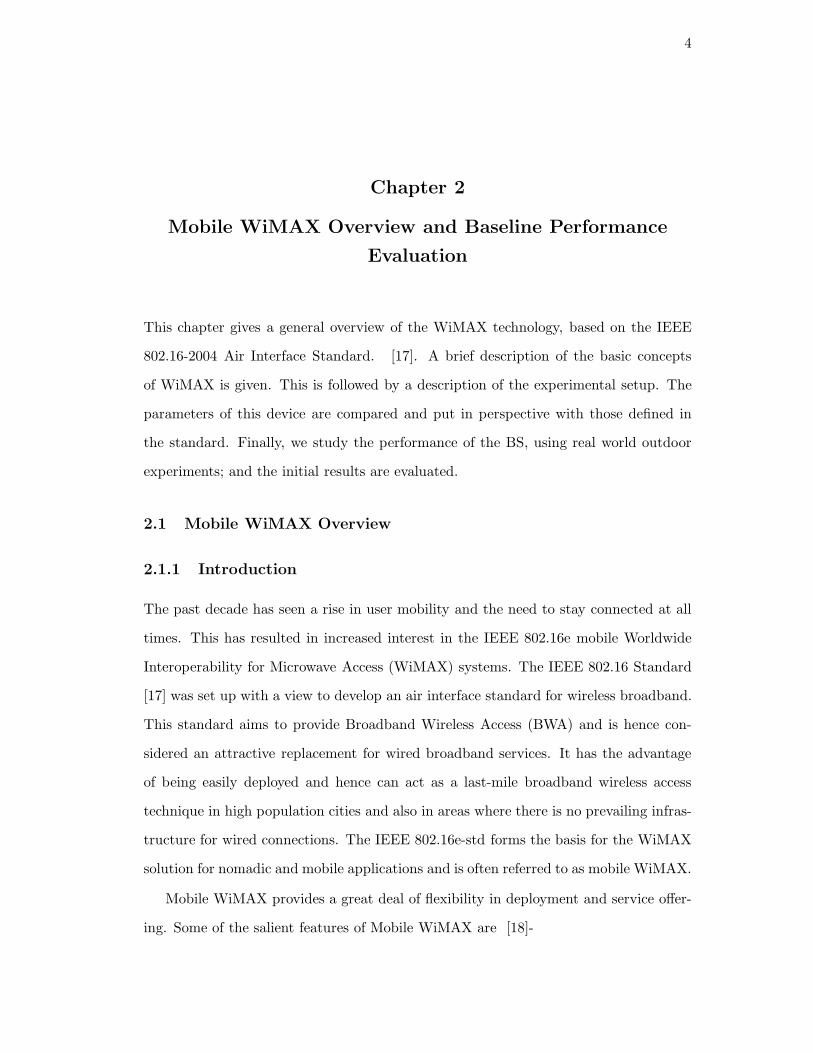
This chapter gives a general overview of the WiMAX technology, based on the IEEE
802.16-2004 Air Interface Standard. [17]. A brief description of the basic concepts
of WiMAX is given. This is followed by a description of the experimental setup. The
parameters of this device are compared and put in perspective with those defined in
the standard. Finally, we study the performance of the BS, using real world outdoor
experiments; and the initial results are evaluated.
2.1 Mobile WiMAX Overview
2.1.1 Introduction
The past decade has seen a rise in user mobility and the need to stay connected at all
times. This has resulted in increased interest in the IEEE 802.16e mobile Worldwide
Interoperability for Microwave Access (WiMAX) systems. The IEEE 802.16 Standard
[17] was set up with a view to develop an air interface standard for wireless broadband.
This standard aims to provide Broadband Wireless Access (BWA) and is hence con-
sidered an attractive replacement for wired broadband services. It has the advantage
of being easily deployed and hence can act as a last-mile broadband wireless access
technique in high population cities and also in areas where there is no prevailing infras-
tructure for wired connections. The IEEE 802.16e-std forms the basis for the WiMAX
solution for nomadic and mobile applications and is often referred to as mobile WiMAX.
Mobile WiMAX provides a great deal of flexibility in deployment and service offer-
ing. Some of the salient features of Mobile WiMAX are [18]-

5
1. High Data Rates:
The inclusion of MIMO antenna techniques along with flexible sub-channelization
schemes, advanced coding and modulation all enable the Mobile WiMAX tech-
nology to achieve peak PHY data rates of around 25Mbps and 6.7Mbps for the
downlink and the uplink, respectively. These peak theoretical PHY data rates are
achieved when using 64 QAM modulations with rate 5/6 error-correction coding,
with a specified DL/UL ratio and bandwidth.
2. Quality of Service (QoS):
One of the main premises of IEEE 802.16 MAC architecture is Quality of Service
(QOS). The MAC layer has a connection oriented architecture which can support
a variety of applications including multimedia services. The system offers specific
support for constant bit rate, variable bit rate, real-time, and non-real-time traffic
flows, in addition to best-effort data traffic. The MAC can support a large number
of multiple connections, each with its own QoS requirement.
3. Scalability bandwidth and data rate support:
WiMAX allows scaling of the data rates depending on current channel condi-
tions. OFDM supports this scalability, through changing the size of the Fast
Fourier Transform based on channel conditions. Different networks have different
bandwidth allocations and scaling is essential to support roaming.
4. Security:
WiMAX has a robust privacy and key management protocol and also supports
encryption using Advanced Encryption Standard (AES) . Provision for authenti-
cation architecture based on Extensible Authentication Protocol is also provided.
This allows for various user credentials like digital certificates, user/name pass-
word, smart cards, etc.
5. Mobility: Mobile WiMAX needs to ensure that real time applications like VoIP
can handle mobility, without significant degradation in service. This is supported

6
using optimized handover schemes that have latencies that are less than 50 mil-
liseconds.
We now take a look at the WiMAX PHY and MAC layers
2.1.2 WiMAX Physical Layer
The WiMAX physical layer is based on orthogonal frequency division multiplexing.
OFDM is ideal for non line of sight (NLOS), high data rate transmissions, OFDM is
used in a number of commercial broadband systems like DSL, Wi-Fi, etc. In OFDM, a
high data rate bit stream is divided into multiple lower data rate bit streams, which are
modulated on separate carriers, which are referred to as tones or subcarriers. OFDM
provides a number of advantages in comparison to other solutions used for transmitting
at high speeds. One of the main factors is the graceful degradation of performance as
the delay spreads exceed the values that it was originally designed for. It is also robust
against narrow band interference and is suitable for coherent demodulation.
The subcarriers can be divided into groups of subcarriers that are referred to as sub
channels. Subchannels can be made from subcarriers that are either pseudo-randomly
generated or are contiguous. Different subchannels can be allocated to different users to
support a multi-access scheme. This scheme is used in Mobile WiMAX and is referred
to as OFDMA. Both uplink and downlink sub channelization is supported in Mobile
WiMAX. Allocating subchannels to users based on their frequency response is termed
as adaptive modulation and coding (AMC).This can be used to enhance the channel
capacity by varying the subchannel according to the signal to noise ratio (SNR) [18].
The Mobile WiMAX air interface supports both TDD and FDD modes [19]. In
the TDD mode, the downlink frame is followed by a small guard interval and then
the uplink frame is transmitted; whereas in the FDD mode, the uplink and downlink
frame are transmitted simultaneously. The TDD mode is usually preferred because
here it is possible to dynamically allocate DL/UL resources to support asymmetric
UL/DL ratio and also, only one channel as compared to the two in FDD. Multiple
users are allocated data regions within the frame and these allocations are specified

7
using UL/DL MAP messages. The MAP messages include the burst profile which
determines the Modulation and Coding scheme that is used in that link. The uplink
subframe comprises of several uplink bursts from different users and also has a channel
quality indicator channel (CQICH) through which the client can send feedback to the
BS.
WiMAX supports a number of modulation and coding schemes like QPSK, 16 QAM
and 64 QAM. It also provides the ability to adaptively vary the modulation scheme
based on channel conditions. The BS can vary the modulation scheme based on channel
quality feedback and received signal strength for downlink and uplink respectively.
The data rate performance of the physical layer varies based on a number of operat-
ing parameters. The channel bandwidth and modulation along with the coding scheme
used play a major rule in influencing the data rate.
2.1.3 WiMAX MAC Layer
The WiMAX MAC layer acts as an interface between the higher transport layer and the
lower physical layer. The MAC layer is responsible for arranging outgoing packets from
the upper layer, called Service Data Units (SDUs) and organizes them into Protocol
Data Units (PDUs) [20]. WiMAX is designed to provide very high data rates and this
is done by providing the flexibility to combine multiple SDUs into a single PDU, to
save on MAC overhead when the SDU size is small; or by partitioning a large SDU into
multiple PDU. Multiple PDUs can also be transmitted simultaneously in a single burst
to avoid PHY overhead.
The MAC protocol is connection oriented, where each SS that enters the network
needs to register with the BS and set up connections which are used for data transfer
with the BS. The BS in turn assigns a unique 16 bit connection identifier (CID) for
each connection. WiMAX also defines the concept of a service flow. This is identified
using a service flow identifier (SFID) and is a unidirectional flow of packets with a
specified QoS. Every CID is mapped to a service flow and a QoS level. The MAC
layer is responsible for assigning air link resources and providing QoS. The BS allocates
resources to all the users for both uplink and downlink. The downlink bandwidth is
8
allocated based on incoming traffic and the downlink bandwidth is allocated based on
the request that is made by the MS via polling by the BS.
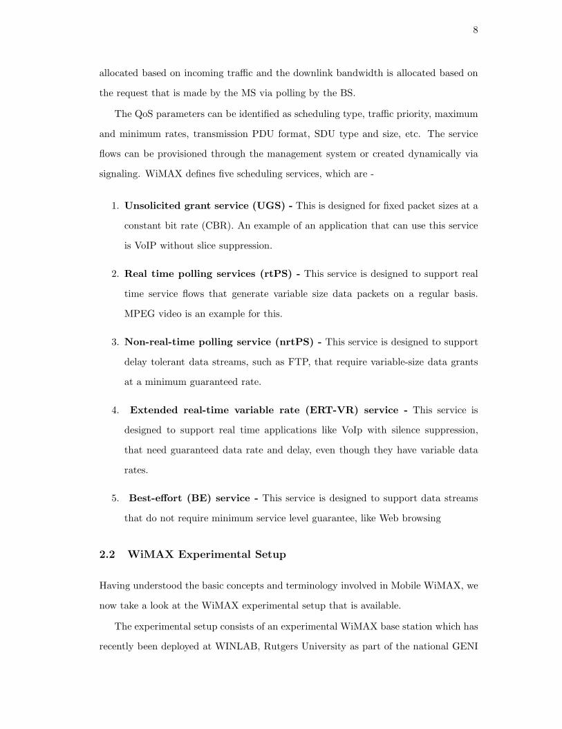
The QoS parameters can be identified as scheduling type, traffic priority, maximum
and minimum rates, transmission PDU format, SDU type and size, etc. The service
flows can be provisioned through the management system or created dynamically via
signaling. WiMAX defines five scheduling services, which are -
1. Unsolicited grant service (UGS) - This is designed for fixed packet sizes at a
constant bit rate (CBR). An example of an application that can use this service
is VoIP without slice suppression.
2. Real time polling services (rtPS) - This service is designed to support real
time service flows that generate variable size data packets on a regular basis.
MPEG video is an example for this.
3. Non-real-time polling service (nrtPS) - This service is designed to support
delay tolerant data streams, such as FTP, that require variable-size data grants
at a minimum guaranteed rate.
4. Extended real-time variable rate (ERT-VR) service - This service is
designed to support real time applications like VoIp with silence suppression,
that need guaranteed data rate and delay, even though they have variable data
rates.
5. Best-effort (BE) service - This service is designed to support data streams
that do not require minimum service level guarantee, like Web browsing
2.2 WiMAX Experimental Setup
Having understood the basic concepts and terminology involved in Mobile WiMAX, we
now take a look at the WiMAX experimental setup that is available.
The experimental setup consists of an experimental WiMAX base station which has
recently been deployed at WINLAB, Rutgers University as part of the national GENI

9
experimental network for future Internet research. This Profile A WiMAX Base Station
is described below-
The NEC Release 1 WiMAX base-station hardware is a 5U rack based system which
consists of multiple Channel Cards (CHC) and a Network Interface Card. The shelf
can be populated with up to three channel cards, each supporting one sector for a
maximum of three sectors. The BS operates in the 2.5 Ghz or the 3.5 Ghz bands and
can be tuned to use either 5, 7 or 10 Mhz channels. At the MAC frame level, 5 msec
frames are supported as per the 802.16e standard. The TDD standard for multiplexing
is supported where the sub-channels for the Downlink (DL) and Uplink (UL) can be
partitioned in multiple time-frequency configurations.
Figure 2.1: NEC WiMAX Base Station hardware configuration [1]
The base-station supports standard adaptive modulation schemes based on QPSK,
16QAM and 64QAM. The interface card provides one Ethernet Interface (10/100/1000)
which will be used to connect to the high performance PC. The base station has been
tested for radio coverage and performance in realistic urban environments and is being
used in early WiMAX deployments.
The 802.16e base station allocates time-frequency resources on the OFDMA link
with a number of service classes as specified in the standard - these include unsolicited
10
grant service (UGS), expedited real time polling service (ertPS), real-time polling ser-
vice (rtPS), non-real time polling (nrtPS) and best effort (BE). The radio module as
currently implemented includes scheduler support for the above service classes in strict
priority order, with round-robin, or weighted round-robin being used to serve multiple
queues within each service class. It is noted that OFDMA in 802.16e with its dy-
namic allocation of time-frequency bursts provides resource management capabilities
qualitatively similar to that of a wired router with multiple traffic classes and priority
based queuing. Also, the 802.16e base station’s signal is compatible with commodity
802.16e mobile platforms (for example, the Samsung M8000, Nokia N800 and Motorola
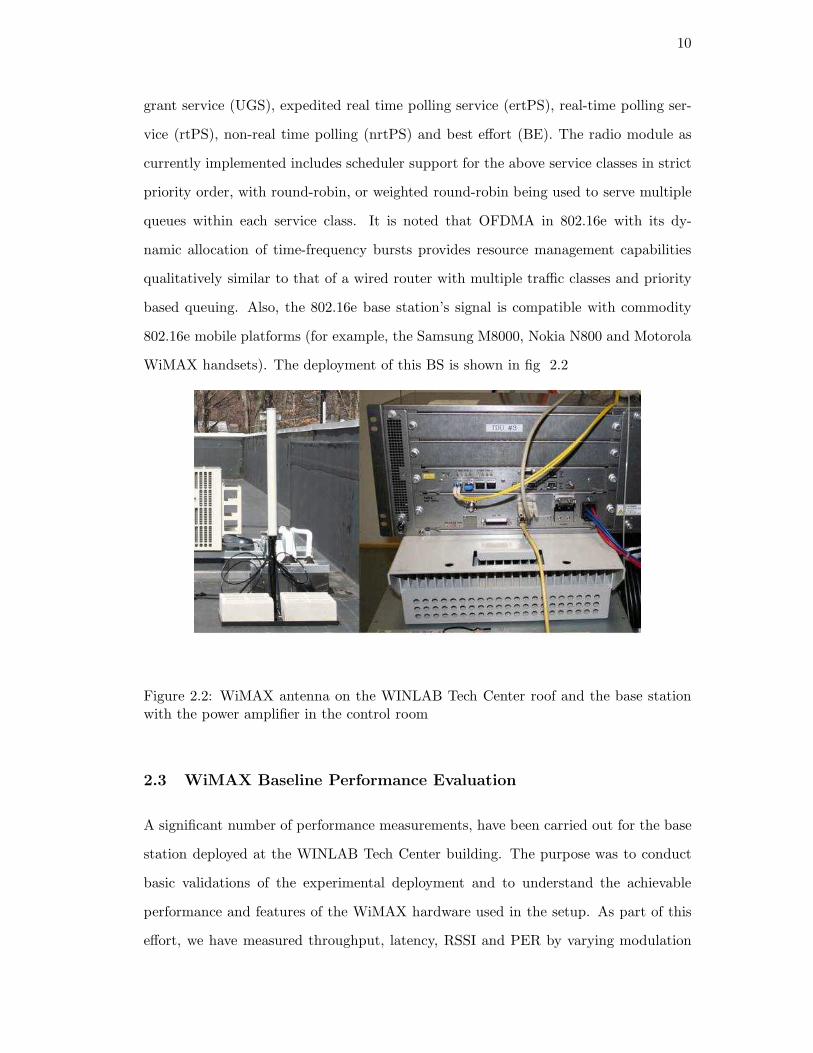
WiMAX handsets). The deployment of this BS is shown in fig 2.2
Figure 2.2: WiMAX antenna on the WINLAB Tech Center roof and the base stationwith the power amplifier in the control room
2.3 WiMAX Baseline Performance Evaluation
A significant number of performance measurements, have been carried out for the base
station deployed at the WINLAB Tech Center building. The purpose was to conduct
basic validations of the experimental deployment and to understand the achievable
performance and features of the WiMAX hardware used in the setup. As part of this
effort, we have measured throughput, latency, RSSI and PER by varying modulation

11
and coding schemes, service classes, receiver locations and performance under mobil-
ity [21]. Some of these experiments and their results are explained below.
2.3.1 WiMAX Coverage Map
This experiment was performed to get a coverage trace and understand the channel
conditions at different points around the BS deployment site. A WiMAX client was
placed in a car, along with a GPS system. A basic drive was performed and the RSSI
values were logged and mapped to the GPS coordinates. A Google Earth image showing
this trace is shown in figure 2.3 .
Figure 2.3: WiMAX BS coverage trace
2.3.2 Location Based Experiment
The next experiment performed was done with the client stationary at 3 different lo-
cations.The locations are of increasing distance from the BS . A Google Earth image
marking these positions exactly, is shown in figure 2.4.

12
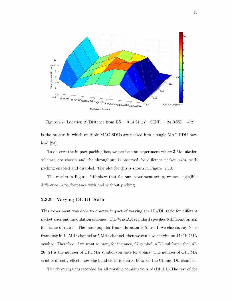
Throughput rates were observed for varying MCSs and packet sizes. The results for
the 3 locations are plotted in Figures 2.5 2.6 2.7 .
Figure 2.4: Experimental scenarion for 2.3.2 marking the points at which the tests arecarried out
In all the cases we observe that link performance improves with increasing packet
sizes. We also observe that in all cases the observed throughput increases with a better
modulation and coding scheme. In Fig 2.5 we see that best performance is achieved
at 64QAM5/6 since channel conditions are the best. For Location-1 we observe that
best performance is achieved at 64QAM2/3. Finally, for Location-2 we observe best
performance at a lower rate of 64QAM1/2. In all cases we observe that the link
adaptation algorithm is able to select the best MCS most of the times leading to a
good performance for varying conditions.
These plots give us baseline throughput measurements at different locations, for
varying packets sizes and MCSs; and act as reference measure for all further experi-
ments.

13
64
128
256
512
1024
64 QAM 5/664 QAM 2/364 QAM 1/216 QAM 3/416 QAM 1/2QPSK 3/4QPSK 1/2Auto0
5
10
15
20
Packet Size (Bytes)
Modulation Scheme
Thr
ough
put (
Mbi
ts/S
ec)
2
4
6
8
10
12
14
16
Figure 2.5: Control Room (Distance from BS = 0.01 Miles)– CINR = 29 RSSI = -51
2.3.3 Link Adaptation Algorithms Evaluation
This experiment was performed to understand the performance of built in link adapta-
tion algorithms. The BS allows to set the Minimum CINR for each Modulation Coding
Scheme (MCS) to be used in Auto switching.This ensures that only when at least the
minimum CINR for that modulation scheme is reached, will that scheme be available.
The MCSs that are used by the Auto Rate Scheme can also be set explicitly. Here,
we see that as the CINR varies from 19 to 31; we select all the modulation schemes
from 1/2 QPSK to 64 QAM 5/6 and compare this with the Auto Rate algorithms.
The BS provides two Auto-Rate algorithms - CQICH and REP-REQ/RSP. The
channel quality information channel (CQICH) is allocated by the BS as soon as the
BS and the SS are informed of each others modulation and coding capabilities, and is
used for periodic CINR (carrier to interference plus noise ratio) reports from the SS to
the BS. Alternatively, the BS may send a REP-REQ message in order to request either
the RSSI (received signal strength indicator) and CINR channel measurements by the
SS, or the results of previously scheduled measurements. The SS responds with the
REP-RSPmessage that contains the corresponding values [22].

14
64
256
512
1024
1400
64 QAM 5/664 QAM 2/3
64 QAM 1/216 QAM 3/4
16 QAM 1/2QPSK 3/4
QPSK 1/2Auto
0
5
10
15
Packet Size (Bytes)
Modulation Scheme
Thr
ough
put (
Mbi
ts/S
ec)
2
4
6
8
10
12
Figure 2.6: Location 1 (Distance from BS = 0.06 Miles)– CINR = 27 RSSI = -67
A path, where the CINR varied from 31 to 19 was chosen, to perform the experi-
ment.The best Modulation Schemes for the two extreme CINRs were chosen, along with
an intermediate MCS and these were compared with the two link adaptation schemes
that were enabled for Downlink, and all the Modulation schemes between the two ex-
tremes were made available. The duration of the walk along the path and back took
a total of 120 seconds. A considerable fluctuation in CINR was observed between the
40 and the 80 second mark. An approximate trace for this path, within WinLab Tech
Ceneter along with a plot of the throughput vs time for various MCSs, is plotted in
Figure 2.8.
The results in Figure 2.9 indicate that auto rate fairs well even in varying channel
conditions and its rates are comparable to the best possible rate the given channel
condition.
2.3.4 Packing vs No-Packing
The BS allows to enable and disable packing of the data units. Fragmentation is the
process in which a MAC SDU is divided into one or more MAC SDU fragments.Packing
15
64
256
512
1024
1400
64 QAM 5/664 QAM 2/364 QAM 1/216 QAM 3/416 QAM 1/2QPSK 3/4QPSK 1/2Auto
0
2
4
6
8
10
12
Packet Size (Bytes)
Modulation Scheme
Thr
ough
put (
Mbi
ts/S
ec)
1
2
3
4
5
6
7
8
9
10
Figure 2.7: Location 2 (Distance from BS = 0.14 Miles)– CINR = 24 RSSI = -72
is the process in which multiple MAC SDUs are packed into a single MAC PDU pay-
load [23].
To observe the impact packing has, we perform an experiment where 3 Modulation
schemes are chosen and the throughput is observed for different packet sizes, with
packing enabled and disabled. The plot for this is shown in Figure 2.10.
The results in Figure. 2.10 show that for our experiment setup, we see negligible
difference in performance with and without packing.
2.3.5 Varying DL-UL Ratio
This experiment was done to observe impact of varying the UL/DL ratio for different
packet sizes and modulation schemes. The WiMAX standard specifies 6 different option
for frame duration. The most popular frame duration is 5 ms. If we choose, say 5 ms
frame say in 10 MHz channel or 5 MHz channel, then we can have maximum 47 OFDMA
symbol. Therefore, if we want to have, for instance, 27 symbol in DL subframe then 47-
26=21 is the number of OFDMA symbol you have for uplink. The number of OFDMA
symbol directly effects how the bandwidth is shared between the UL and DL channels.
The throughput is recorded for all possible combinations of (DL,UL).The rest of the

16
Figure 2.8: A trace of the path chosen for the experiment, and the corresponding RSSIfor the duration of the walk.
parameters are kept constant. The results are provided in Figure. 2.11.
We observe that throughput scales with different packet sizes as observed earlier.
As the DL-UL ratio is increased we see an increase in the downlink throughput. It is
also observed that this impact is greatest for large packet sizes and vice versa. The
results confirm with the theoretical values, and hence provide us with a mechanism to
control the division of channel between uplink and downlink.

17
10 20 30 40 50 60 70 80 90 100 110 1200
2
4
6
8
10
12
14
16
18
Time (Seconds)
Thr
ough
put (
Mbi
ts/S
ec)
Auto (CQICH)16 QAM 1/264 QAM 2/364 QAM 5/6Auto (REP−REQ/RSP)
Figure 2.9: Comparision of Auto-Rate with other Modulation Schemes
32 64 128 256 512 10240
2
4
6
8
10
12
14
16
18
Packet Size ( Bytes )
Thr
ough
put (
Mbi
ts/S
ec )
64 QAM 5/6 Packing64 QAM 5/6 No−PackingHalf QPSK PackingHalf QPSK No Packing16 QAM 3/4 Packing16 QAM 3/4 No Packing
Figure 2.10: A comparison of Packing enabled and disabled for various MCSs andpacket sizes.

18
(35,12)
(32,15)
(29,18)
(26,21)
3264
128256
5121024
2
4
6
8
10
12
14
16
Num of OFDMA Symbols (DL, UL)Packet Size (Bytes)
Thr
ough
put (
Mbi
ts/S
ec)
4
6
8
10
12
14
Figure 2.11: Impact of UL-DL ration on throughput rates.

19
Chapter 3
Virtualization
This chapter begins by providing an overview of the various virtualization techniques
that are available. This is followed by a discussion about the Kernel Virtual Machine
(KVM), which we use for creating slices for the BS. This is followed by some basic
experiments to test the performance of KVM. The results of these experiments are
studied.
3.1 Virtualization Basics
Virtualization is a framework or methodology of dividing the resources of a computer
into multiple execution environments, by applying one or more concepts or technologies
such as hardware and software partitioning, time-sharing, partial or complete machine
simulation, emulation, quality of service, and many others [24]. Simply put, to virtual-
ize, means to take something of one form and make it appear to be another form.
The general process of virtualization can be best explained with the help of the
following diagram [25]-
Figure 3.1: Layered abstraction of virtualization [2]

20
The hardware machine that needs to be virtualized forms the bottom of the vir-
tualization solution. Virtualization may or may not be supported on this machine
directly. The next layer above this is comprised of the hypervisor of the Virtual Ma-
chine Manager (VMM). This layer acts as an abstraction between the operating system
and the hardware. If the functions of the hypervisor are performed by the operating
system itself, then this operating system is called the host operating system. The ac-
tual virtual machines (VMs) form the final layer of the virtualization solution. These
VMs are isolated operating systems, and are provided with the illusion that the host
hardware platform belongs to them. These VMs are independent devices and can have
applications that might be associated with it.
Having understood what virtualization is, we take a look at the different types of
virtualization techniques that are possible [2] -
1. Hardware emulation
Figure 3.2: Hardware emulation [2]
In this technique, the virtualization is provided by creating virtual machines that
emulate the hardware of interest. This technique allows for the operating system
to run completely unmodified. The main drawback of this is that it is very slow.
Examples of hardware emulation is QEMU. Figure 3.2 shows the basic blocks of
Hardware Emulation.
2. Full virtualization

21
Figure 3.3: Full virtualization [2]
This mode of virtualization uses a virtual machine manager to mediate between
the guest operating system and the host hardware. This requires some protected
instructions to be trapped and handled by the VMM, since the underlying hard-
ware is shared by all the virtual machines. This technique also allows the OS to
run unmodified, but it does need to be compatible with the underlying hardware.
VMware and z/VM are examples of this. This technique is explained in 3.3
3. Paravirtualization
Figure 3.4: Paravirtualization [2]
This method is similar to full virtualization; wherein it uses a hypervisor to me-
diate access to the hardware; but it requires that the guest operating system

22
has some virtualization-aware code present in it. Figure 3.4 explains this tech-
nique.This mechanism does away with the need to trap any privileged instructions,
since the guest OS is aware of the virtualization process. Paravirtualization comes
closest to offering performance that is close to that of an unvirtualized system.
Xen and UML make use of the paravirtualization technique.
4. Operating system-level virtualization
Figure 3.5: Operating system-level virtualization block diagram [2]
The final technique that we look at, in figure 3.6 virtualizes server on the top of
the operating system itself. This method isolates the independent servers from
each other, while supporting the same operating system to be used by them. This
can provide native performance at the cost of changes to the operating system
kernel.
3.2 Base Station Virtualization
The concepts studied in the previous section lay the groundwork to understand the
requirements of virtualization and the technique used in this process.
3.2.1 Why is virtualization needed?
Virtualization allows a single machine/node to implement multiple instances of a re-
quired logical resource within the same or different slices. One of the main challenges
with the current basestation is to provide a setup where multiple experimenters could

23
run experiments which involve a WiMAX basestation and clients as a part of their
experimentation setup.
The most basic step involved in achieving this configuration is to setup virtual
containers using one of the techniques described in the previous section
3.2.2 Kernel Virtual Machine (KVM)
KVM is a virtualization technique that uses a kernel module to turn the Linux kernel
into a hypervisor [26].This is the first virtualization technique that is a part of the main
Linux kernel. The guest operating systems can run in user-space of the host Linux
kernel with the help of this module. Each guest operating system is a single process of
the host operating system (or hypervisor).
A new execution mode, guest mode; is introduced into the kernel by the KVM
module. Plain kernel supports just kernel and user modes.
The guest mode of the kernel is supported by the kernel module exporting a device
called /dev/kvm. This device provides a VM with its own address space, that is separate
from the kernel or any other VM. The devices in the device tree are common to all user
space applications but isolation is provided by providing a different map for /dev/kvm,
for each process that opens it. The physical memory that is mapped for the guest
operating system is actually virtual memory mapped into the process. Translation
from guest physical address to host physical address is provided by maintaining a set
of shadow pages.
KVM is a part of the virtualization solution. The ability to virtualize the processor
for multiple OSes is provided by the processor itself. As discussed earlier, the memory
is virtualized by KVM. Modifying and executing a QEMU process on each operating
system process enables I/O virtualization. QEMU is a platform virtualization solution
that allows virtualization of an entire PC environment.
Figure 3.6 provides a view of virtualization with KVM.
The bottom-most layer is the hardware that is capable of virtualization. The next
layer is provided by the Linux kernel with the KVM module, which acts as a hypervisor.
The Linux kernel supports guest operating system, which is loaded through the kvm

24
Figure 3.6: The virtualization components with Kernel Virtual Machine (KVM)
utility; while also providing support to run applications just like any other Linux kernel.
The guest operating system that is running on the top can run any applications just
like the host operating system.
The main advantage of KVM is that it uses the Linux Kernel as the hypervisor
and hence any changes to the standard Kernel benefit both the host(hypervisor) and
the guest operating system. The drawback of this system involve the need for a user-
space QEMU process, that can provide I/O virtualization, and also the need for a
virtualization capable processor.
3.3 KVM Virtualization Measurements and Observations
KVM is used to create virtual machines on an external machine. This technique allows
us to create containers that can be used to access the WiMAX BS. Resources can be
allocated to these slices, to allow independent experiments to run simultaneously on
the BS. A basic performance evaluation of KVM, with multiple virtual machines is
provided here, and is compared with the performance of the host system; in order to
gauge the performance overhead of operating from a KVM guest system.
3.3.1 KVM Delay Measurements
The most basic measure of performance is the Average Round Trip Delay Time. An
experiment is performed, where the round trip delay times for a single and multiple

25
Host1VM
2 VMs
64
256
512
1024
0
20
40
60
80
100
Packet Size(bytes)
Avg
. Del
ay T
imes
(m
s)
Figure 3.7: KVM Delay measurements with varying packet sizes
virtual machines are measured; for increasing packets sizes. These values are compared
with the host system. Next, this experiment is repeated with the packets size fixed,
with increasing the number of packets transmitted per second. The results of these
experiments are presented in Figures 3.7 and 3.8.
Host1 VM
2 VMs
12
35
10
0
20
40
60
80
100
Number of packets/Sec
Avg
. Del
ay T
imes
Figure 3.8: KVM Delay measurements with varying number of packets per second
These numbers indicate that the overhead of using the KVM virtual machine, as
compared to the host, is minimal.

26
Figure 3.9: KVM Throughput measurements with 2 VM instances - VM1 runningincreasing traffic from 3-5 Mbps and VM2 constant at 10 Mbps.
3.3.2 KVM Throughput Measurements
This experiment is performed to observe the sharing of resources between the slices
created by KVM. For this, an experiment is performed where the the first virtual
machine is running traffic that increases in steps from 2 Mbps to 8 Mbps. The second
VM is running at constant rate of 8 Mbps. The packets size is 1024 and the MCS is
64QAM5/6.
The results in Figure 3.9 show that the 2 clients share the link, until saturation
is reached at around 15.5 Mbps. Here, the VM running at a higher rate; drops to
accommodate the needs of the other VM; until the rate required by the each client
goes above half the saturation rate. This is when the 2 VMs get an equal rate of half
the saturation limit. This shows that the use of KVM does not cause any unfairness
amongst multiple clients, while operating in similar channel conditions.

27
Chapter 4
Ensuring Fairness in Virtual Networks
The Primary goal of virtualizing the WiMAX BS, has been to enable support for mul-
tiple experiments. Having observed the basic performance of the virtualization in sta-
tionary conditions; in the previous chapter, we now observe the performance of vir-
tualization, with varying channel conditions at the mobile device. These experiments
provide a more realistic scenario,; and help us gauge the sharing of resources amongst
multiple slices. Our observations indicate a need for a control mechanism, to ensure
fairness in resource utilization. This control mechanism is proposed in the form of a
Virtual Network Traffic Shaping technique. The implementation details and the impact
this has on fairness between slices; is presented in this chapter.
4.1 Motivation
To justify the need for an air time fairness mechanism, we report some preliminary
measurements with the WiMAX basestation (BS). We begin with a brief description
of the experiment apparatus followed by a pilot experiment to motivate the study.
Parameter V alue
Channel Rate AdaptiveOperation Mode 802.11e
Frequency 2.59GHzDL/UL Ratio 35 : 12
Bandwidth 10MhzClient Chipset Beceem
Table 4.1: Basestation (BS) settings for all experiments. Explicit change in parametersare as mentioned in the experiments.

28
4.1.1 Hardware Setup
All experiments are performed on a Profile A WiMAX BS from NEC Corp. deployed
at the Rutgers University, WINLAB campus. The BS is capable of up to 8 modulation
and coding schemes and implements two mechanisms for downlink rate adaptation.
Link adaptation is done at an interval of 200frames, which can be changed. BS settings
used for all experiments unless mentioned otherwise are as shown in Figure 4.1.
To study the impact of varying channel conditions, on the performance of mobile
clients; an experimental setup comprising 2 clients; 1 stationary and 1 mobile is chosen.
The channel conditions for the mobile client is varied over a given time frame, by walking
on a path within the Winlab Campus is chosen. This path, which takes around 100-120
seconds to complete, with average walking speeds, shows a variation in Received Signal
Strength (RSSI) from -50 to -75 dBm and a variation in CINR from 19 to 31 dB. This
path is the same as the one showing in Figure 2.8, presented in Chapter 2.
The stationary Client is operating in optimal channel conditions with an RSSI of
-50 and CINR at 31. These channel conditions allow the stationary client to operate at
64 QAM5/6 MCS throughout the experiment.
Two KVM Virtual Machines(VM 1 and VM 2) are set up. These machines send
a specified type of traffic, to the WiMAX client at a given rate and frame size. The
throughput values are measured at the Client.
4.1.2 Varying Channel Conditions
In our first measurement, we measure baseline performance of the virtualized wimax
system with two slices. The virtual machines VM1 and VM2 are sending traffic to
clients 1 and 2 respectively. Hence the link from each VM to the corresponding client
constitutes of a slice. Client 1 is kept stationary where it has a CINR greater than
28 which allows the basestation to send traffic comfortably at 64QAM5/6. An exper-
imenter walks with the other client (client 2) as per the coverage map shown in the
figure 2.8 . The observed downlink throughput for both the clients is as shown in Fig-
ure 4.1. We observe that as the mobile client reaches areas where the RSSI drops below
29
certain threshold, the rate adaptation scheme at the basestation selects a more robust
modulation and coding scheme(MCS). However, in the process the link with the mobile
client ends up consuming a lot more radio resource at the basestation, which in turn
affects the performance of the stationary client.
For simplicity, we will consider the initial problem of equal allocation of basestation
resources to each slice. A conservative approach to this problem is through static
shaping. Assuming that we have some way of knowing about the movement of the
mobile client, we could calculate throughput based on 50% channel time at the slowest
MCS. In this case, the basestation uses 1/2QPSK when link quality deteriorates the
most. Hence we use this information to statically shape the throughput of the slice
with the mobile client. The goal of this shaping mechanism is to limit the offered load
for the slice in such a way, that the slice can use only the allocated share of basestation
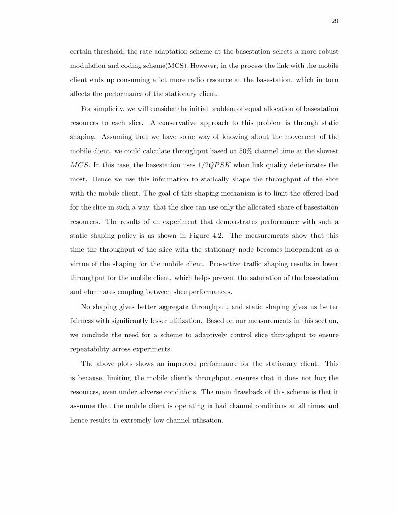
resources. The results of an experiment that demonstrates performance with such a
static shaping policy is as shown in Figure 4.2. The measurements show that this
time the throughput of the slice with the stationary node becomes independent as a
virtue of the shaping for the mobile client. Pro-active traffic shaping results in lower
throughput for the mobile client, which helps prevent the saturation of the basestation
and eliminates coupling between slice performances.
No shaping gives better aggregate throughput, and static shaping gives us better
fairness with significantly lesser utilization. Based on our measurements in this section,
we conclude the need for a scheme to adaptively control slice throughput to ensure
repeatability across experiments.
The above plots shows an improved performance for the stationary client. This
is because, limiting the mobile client’s throughput, ensures that it does not hog the
resources, even under adverse conditions. The main drawback of this scheme is that it
assumes that the mobile client is operating in bad channel conditions at all times and
hence results in extremely low channel utlisation.

30
10 20 30 40 50 60 70 80 90 1000
1
2
3
4
5
6
7
8
9
Time (Seconds)
Thr
ough
put (
Mbp
s)
Stationary ClientMobile Client
Figure 4.1: Mobility experiment - no shaping
4.1.3 Need for control mechanism
The above two subsections presented the results of two experiments, one in which there
is no shaping and the other in which the mobile client is shaped dynamically. The
first experiment shows a very close coupling between the operation of the clients, even
though they are operating in different channel conditions. The second experiment limits
the coupling effect, but results in low channel utlisation.
From the above results, we conclude the need for a scheme to adaptively control
slice throughput to ensure repeatability across experiments. It is also important to
ensure that the amount of BS resources that are being used by each slice, remains as
even as possible. This mechanism is proposed in the next section.
4.2 Virtual Network Traffic Shaping (VNTS) technique
In the previous section, we evaluated the results of mobility in experiments in the
virtualized scenario. These results indicated a need for an adaptive control mechanism,
that can dynamically make decisions, based on the channel conditions that the client
is operating in, at that point of time. In this section, we propose a traffic shaping

31
20 40 60 80 1000
1
2
3
4
5
6
7
Time (Seconds)
Thr
ough
put (
Mbp
s)
Stationary ClientMobile Client
Figure 4.2: Mobility experiment - Static shaping performance.
technique called VNTS, that tries to achieve the goal of ensuring fairness and reducing
coupling; between the clients.
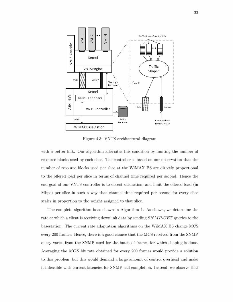
4.2.1 VNTS Architecture
In order to implement the VNTS technique, we propose to run the control mechanism
from the Application Service Network gateway (ASN −GW ). The ASN-GW will have
a VNTS Controller running, that will query the BS and make shaping decisions, based
on the current channel conditions. These decisions will be implemented by the VNTS
Engine, running on an external machine. This machine will have an implantation of
KVM, that provides multiple VMs,which act as multiple containers providing access to
the Base Station. Each container will map to one WiMAX client and traffic destined for
the client, will pass through the host machine. This machine will capture the outgoing
packets and shape them according to the decisions sent by the VNTS Controller.
A diagram showing the details of the architecture is presented in Figure. 4.3.
The different modules of the VNTS technique; the VNTS Controller and the VNTS
engine are explained in the following two sections.

32
Modulation Coding Rate (kbps)
64QAM 5/6 1610064QAM 3/4 1450064QAM 2/3 1380064QAM 1/2 1070016QAM 3/4 1070016QAM 1/2 7180QPSK 3/4 5390QPSK 1/2 3580
Table 4.2: Baseline shaping rates used for deriving shaping rates for individual clients.Observed rates for different modulation and coding schemes are based on results fromexperiments.
4.2.2 VNTS Engine
The control parameter for VNTS is downlink throughput. The shaping of the downlink
throughput is implemented in the VNTS Engine. This shaping is implemented, based
on decisions from the VNTS Controller.
This VNTS Engine is responsible for-
1. Separating VM traffic based on a slice identifiers. We are currently using MAC
identifiers of virtual machine interfaces as the slice identifiers.
2. Routing and shaping all policies to and from the virtual machines.
3. Providing element handlers that allow dynamic control of virtual machine traffic
through an external control mechanism.
The VNTS Engine is implemented using Click Modular Router [27]. A simple block
diagram of the VNTS functions is provided in 4.4. The details of this implementation,
along with an overview of Click ; are provided in Appendix A.
4.2.3 VNTS Controller
The VNTS controller has to determine and set slice throughput on the fly, by considering
current operating conditions. Isolation between slices is compromised when the WiMAX
basestation runs out of resource blocks and the slice with a poor link, eats into a slice
33
Figure 4.3: VNTS architectural diagram
with a better link. Our algorithm alleviates this condition by limiting the number of
resource blocks used by each slice. The controller is based on our observation that the
number of resource blocks used per slice at the WiMAX BS are directly proportional
to the offered load per slice in terms of channel time required per second. Hence the
end goal of our VNTS controller is to detect saturation, and limit the offered load (in
Mbps) per slice in such a way that channel time required per second for every slice
scales in proportion to the weight assigned to that slice.
The complete algorithm is as shown in Algorithm 1. As shown, we determine the
rate at which a client is receiving downlink data by sending SNMP -GET queries to the
basestation. The current rate adaptation algorithms on the WiMAX BS change MCS
every 200 frames. Hence, there is a good chance that the MCS received from the SNMP
query varies from the SNMP used for the batch of frames for which shaping is done.
Averaging the MCS bit rate obtained for every 200 frames would provide a solution
to this problem, but this would demand a large amount of control overhead and make
it infeasible with current latencies for SNMP call completion. Instead, we observe that

34
Figure 4.4: VNTS engine block diagram
as long as the channel does not change a lot over our control loop of 1sec, we will be
able to get an MCS bit rate estimation that is close to the actual MCS used by the
BS. Based on this idea, the control algorithm scales the saturation throughput for slices
in proportion to their weights. The Set() function is used to remotely set throughput
limit for each virtual machine. This loop is executed every second, to achieve repeated
control. The sleep duration for the loop can eventually be made adaptive based on
observed link conditions.
4.3 Evaluation
In this section we evaluate the baseline performance of the VNTS architecture. Various
experiments are conducted and the fairness and aggregate throughput is observed.
4.3.1 Metrics
In our evaluations, we modify and use the Jain fairness index [28] for evaluating weighted
fairness across flows. Let the throughput observed for a slice at the client i be given
by Ti, bit rate achieved with the current modulation and coding scheme for the slice i
35
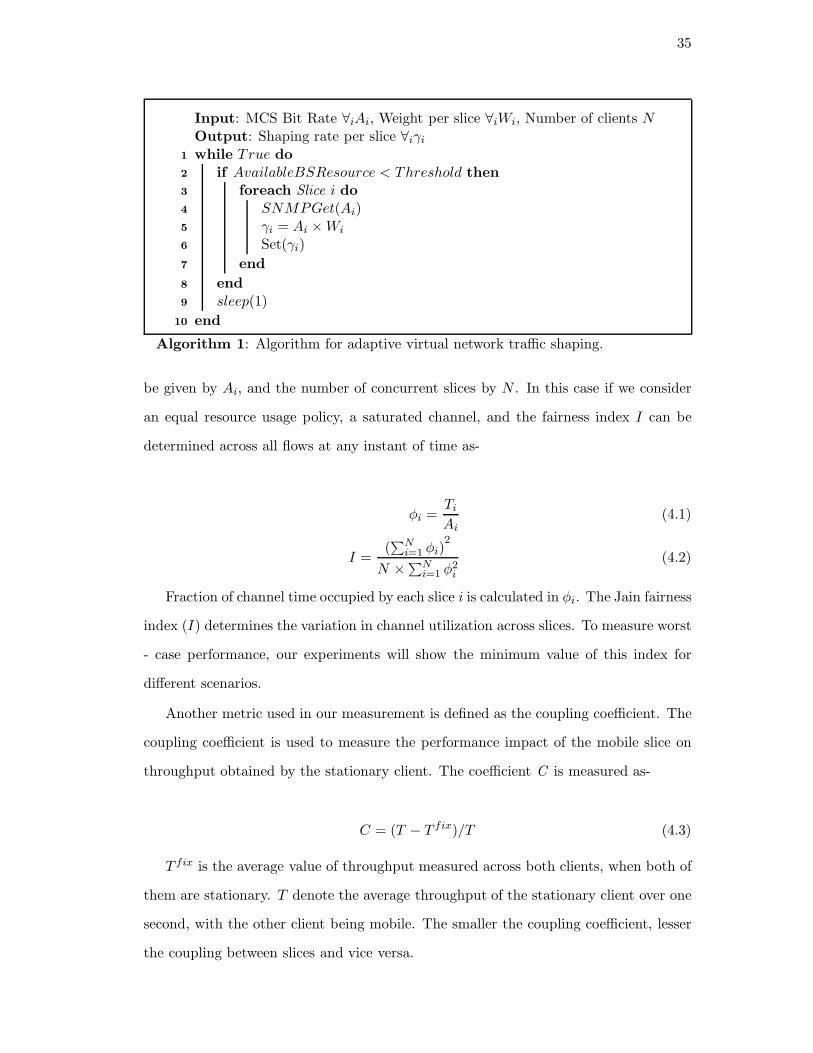
Input: MCS Bit Rate ∀iAi, Weight per slice ∀iWi, Number of clients NOutput: Shaping rate per slice ∀iγi
while True do1
if AvailableBSResource < Threshold then2
foreach Slice i do3
SNMPGet(Ai)4
γi = Ai × Wi5
Set(γi)6
end7
end8
sleep(1)9
end10
Algorithm 1: Algorithm for adaptive virtual network traffic shaping.
be given by Ai, and the number of concurrent slices by N . In this case if we consider
an equal resource usage policy, a saturated channel, and the fairness index I can be
determined across all flows at any instant of time as-
φi =Ti
Ai
(4.1)
I =(∑N
i=1φi)
2
N ×∑N
i=1 φ2
i
(4.2)
Fraction of channel time occupied by each slice i is calculated in φi. The Jain fairness
index (I) determines the variation in channel utilization across slices. To measure worst
- case performance, our experiments will show the minimum value of this index for
different scenarios.
Another metric used in our measurement is defined as the coupling coefficient. The
coupling coefficient is used to measure the performance impact of the mobile slice on
throughput obtained by the stationary client. The coefficient C is measured as-
C = (T − T fix)/T (4.3)
T fix is the average value of throughput measured across both clients, when both of
them are stationary. T denote the average throughput of the stationary client over one
second, with the other client being mobile. The smaller the coupling coefficient, lesser
the coupling between slices and vice versa.
36
In our measurements we focus on improving the worst case performance. Hence
we will plot the maximum value of the coupling index seen over the duration of the
experiments in all measurements.
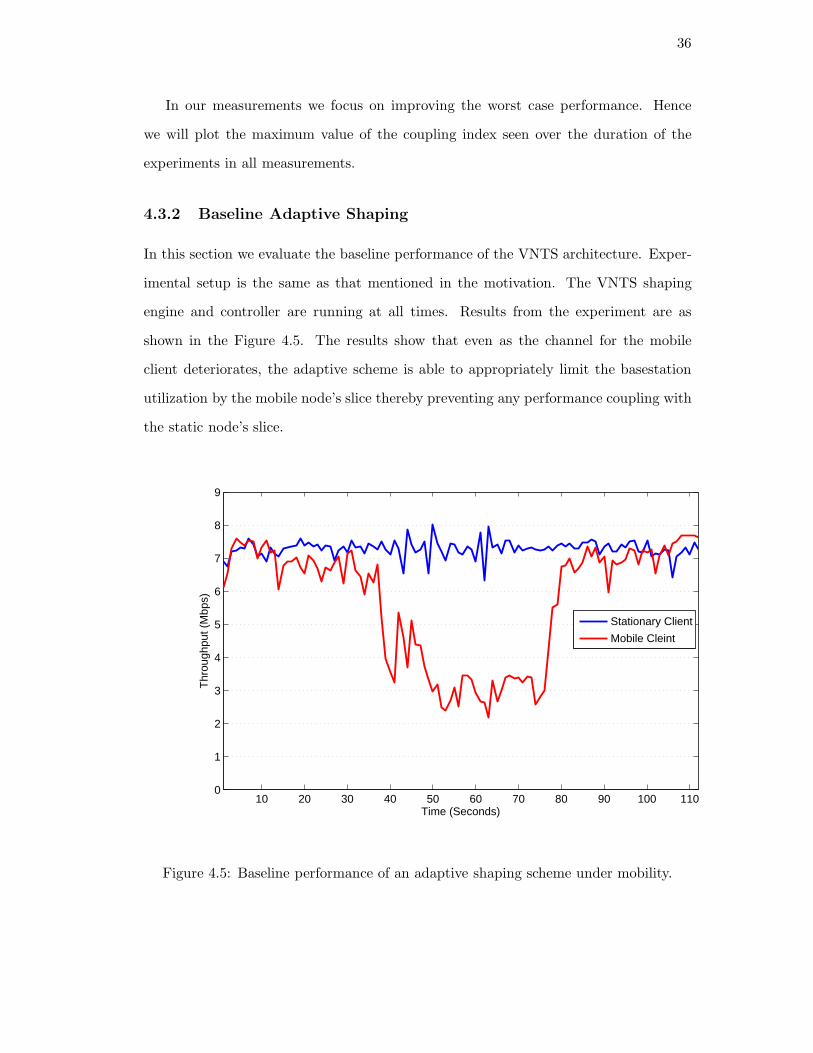
4.3.2 Baseline Adaptive Shaping
In this section we evaluate the baseline performance of the VNTS architecture. Exper-
imental setup is the same as that mentioned in the motivation. The VNTS shaping
engine and controller are running at all times. Results from the experiment are as
shown in the Figure 4.5. The results show that even as the channel for the mobile
client deteriorates, the adaptive scheme is able to appropriately limit the basestation
utilization by the mobile node’s slice thereby preventing any performance coupling with
the static node’s slice.
10 20 30 40 50 60 70 80 90 100 1100
1
2
3
4
5
6
7
8
9
Time (Seconds)
Thr
ough
put (
Mbp
s)
Stationary Client
Mobile Cleint
Figure 4.5: Baseline performance of an adaptive shaping scheme under mobility.

37
4.3.3 Varying Policies
Performance obtained with the adaptive shaping mechanism is also dependent on the
conservativeness of the shaping algorithm. Shaping resource utilization to more con-
servative values will enable better performance isolation between slices. However, this
will also lead to a lesser net utilization of the available resources.
4 10 14 200.5
0.6
0.7
0.8
0.9
1
Aggregate Load (Mbps)
Min
imum
− F
airn
ess
Inde
x
No ShapingVNTS at Experimental ValuesVNTS at 10% Experimental ValuesVNTS at 20% Experimental Values
Figure 4.6: Various shaping policies - Minimum Fairness Index.
In our experiment we will vary the conservativeness of our adaptive mapping algo-
rithm. We measure performances by shaping at 80%, 90% and 100% of the prescribed
channel rates for each of the modulation and coding schemes. We repeat the same
experiment as in the previous section, by having a mobile client and stationary client
and measuring throughput and resource usage across the experiment.
Figure 4.6 and figure 4.7 plot the minimum and average value of the Fairness index
for each slice based on the basestation resources promised to each slice as a function
of aggregate load on the system. When we are not doing any shaping the fairness
index hits a low of 0.67. However, with adaptive shaping at 80%, 90% and 100% we
see the index ranging from 0.84 − −0.97 while being independent of the system load.

38
4 10 14 200.95
0.96
0.97
0.98
0.99
1
Aggregate Load (Mbps)
Ave
rage
− F
airn
ess
Inde
x
No ShapingVNTS at Experimental ValuesVNTS at 90% Experimental ValuesVNTS at 80% exoerimental Values
Figure 4.7: Various shaping policies - Average Fairness Index.
We also see an improvement of up to 30% for certain system loads and shaping policy
combinations. Since we do not see a significant difference in fairness performance across
policies we use aggregate throughput as a metric for deciding the best shaping rates.
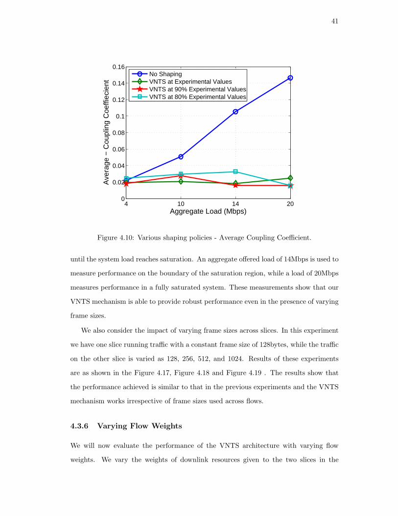
Figures 4.9 and 4.10 plot the worst case and average coupling factors. It is seen
that the coupling factor is reduced from 0.68 to around 0.1 – 0.2 using the VNTS
shaping.
Figure 4.8 shows the total aggregate throughput of the slices as a function of aggre-
gate offered load. It is seen that the aggregate throughput across all system loads is the
best when we use the prescribed channel rates without making the policy conservative.
This makes the default rates a favored pick for all the remaining experiments.
4.3.4 Vehicular Measurements
To further validate the working of our VNTS system, we perform experiments with the
mobile client placed in a vehicle. Experiment setup is same as that in the previous
sections, with the exception that performance is determined only under saturation con-
ditions, where each slice has an offered load of 10Mbps. Outdoor results are measured

39
4 10 14 202
4
6
8
10
12
14
Aggregate Load (Mbps)
Agg
rega
te T
hrou
ghpu
t (M
bps)
No ShapingVNTS at Experimental ValuesVNTS at 90% Experimental ValuesVNTS at 80% Experimental Values
Figure 4.8: Various shaping policies - Observed aggregate link throughput.
for two topologies (Topo-2,3 ) as shown in Figure 4.11.
Average velocity of the vehicle is maintained greater than 10Mph for both Topo-
2,3. These results are compared with those obtained from the indoor experiment Topo-1
topology shown in Figure 2.8.
Figure 4.12 shows the results with our modified fairness index for the three exper-
iment setups. We observe that in all the cases, we obtain better fairness using our
VNTS mechanism. We observe that while the average values of the fairness index show
small improvements across the three topologies, the worst case performance (minimum
fairness points) is significantly improved with the use of our shaping mechanism. Fig-
ure 4.13 plots the performance of the coupling factor for the three topologies. Coupling
factor values are shown for both average and worst case conditions. In the average
case, we observe that the coupling reduces for all topologies with the use of our VNTS
mechanism. The VNTS mechanism also improves the worst case performance for all
topologies with reduction in coupling of up to 40% in some cases. Thus, using our
VNTS mechanism, we are able to significantly improve fairness across slices even when

40
4 10 14 200
0.1
0.2
0.3
0.4
0.5
0.6
0.7
Aggregate Load (Mbps)
Max
imum
− C
oupl
ing
Coe
ffiec
ient
No ShapingVNTS at Experimental ValuesVNTS at 90% Experimental ValuesVNTS at 80% Experimental Values
Figure 4.9: Various shaping policies - Maximum Coupling Coefficient.
one of the nodes is moved in a vehicle.
4.3.5 Varying Frame Sizes
From the evaluation in the previous experiments we see that fairness index improves
significantly after using our adaptive shaping mechanism. We will now evaluate the
performance of our system in the presence of varying frame sizes for slices. Frame sizes
are varied simultaneously for both slices. Initially, Frame sizes are varied as 128, 256, 512
and 1024Bytes. Results from the experiment are plotted in Figure 4.14, Figure 4.15
and Figure 4.16 as a function of increasing aggregate offered load.
The minimum value of the Jain fairness index varies from 0.77 − 0.87. However,
we do not see a pattern which hints towards a correlation with frame size. Also, the
relatively high variance in the index value during the course of an experiment rules
out any correlation between frame size and observed fairness. Figure 4.16 shows that
the coupling factor is limited to below 0.3, for all packet sizes. Observation from
Figure 4.15 shows that the aggregate throughput does not vary much with frame sizes
41
4 10 14 200
0.02
0.04
0.06
0.08
0.1
0.12
0.14
0.16
Aggregate Load (Mbps)
Ave
rage
− C
oupl
ing
Coe
ffiec
ient
No ShapingVNTS at Experimental ValuesVNTS at 90% Experimental ValuesVNTS at 80% Experimental Values
Figure 4.10: Various shaping policies - Average Coupling Coefficient.
until the system load reaches saturation. An aggregate offered load of 14Mbps is used to
measure performance on the boundary of the saturation region, while a load of 20Mbps
measures performance in a fully saturated system. These measurements show that our
VNTS mechanism is able to provide robust performance even in the presence of varying
frame sizes.
We also consider the impact of varying frame sizes across slices. In this experiment
we have one slice running traffic with a constant frame size of 128bytes, while the traffic
on the other slice is varied as 128, 256, 512, and 1024. Results of these experiments
are as shown in the Figure 4.17, Figure 4.18 and Figure 4.19 . The results show that
the performance achieved is similar to that in the previous experiments and the VNTS
mechanism works irrespective of frame sizes used across flows.
4.3.6 Varying Flow Weights
We will now evaluate the performance of the VNTS architecture with varying flow
weights. We vary the weights of downlink resources given to the two slices in the
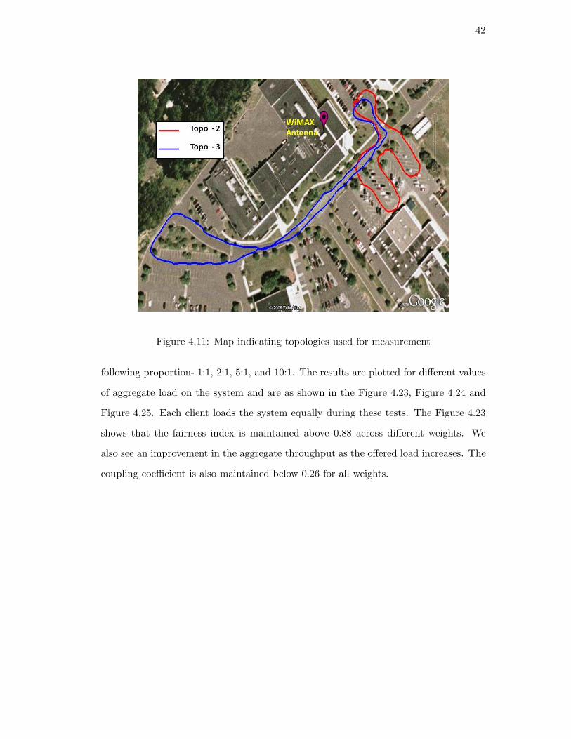
42
Figure 4.11: Map indicating topologies used for measurement
following proportion- 1:1, 2:1, 5:1, and 10:1. The results are plotted for different values
of aggregate load on the system and are as shown in the Figure 4.23, Figure 4.24 and
Figure 4.25. Each client loads the system equally during these tests. The Figure 4.23
shows that the fairness index is maintained above 0.88 across different weights. We
also see an improvement in the aggregate throughput as the offered load increases. The
coupling coefficient is also maintained below 0.26 for all weights.

43
Topo − 1 Topo − 2 Topo − 30
0.2
0.4
0.6
0.8
1
Topologies
Fai
rnes
s In
dex
No Shaping − AvgNo Shaping − MinShaping − AvgShaping − Min
Figure 4.12: Fairness Index for topologies used in Vehicular Measurements
Topo − 1 Topo − 2 Topo − 30
0.1
0.2
0.3
0.4
0.5
0.6
0.7
Topologies
Cou
plin
g C
oeffi
ecie
nt
No Shaping − AvgNo Shaping − MaxVNTS − AvgVNTS − Max
Figure 4.13: Coupling Coefficient for topologies used in Vehicular Measurements

44
4 10 14 200.5
0.55
0.6
0.65
0.7
0.75
0.8
0.85
0.9
0.95
1
Aggregate Load (Mbps)
Min
imum
− F
airn
ess
Inde
x
Packet Size − 128 BytesPacket Size − 256 BytesPacket Size − 512 BytesPacket Size − 1024 Bytes
Figure 4.14: Minimum value of Fairness Index for different frame sizes.
4 10 14 203
4
5
6
7
8
9
10
11
12
13
Aggregate Load (Mbps)
Agg
rega
te T
hrou
ghpu
t (M
bps)
Packet Size − 128 BytesPacket Size − 256 BytesPacket Size − 512 BytesPacket Size − 1024 Bytes
Figure 4.15: Observed aggregate link throughput for different frame sizes.

45
4 10 14 200
0.05
0.1
0.15
0.2
0.25
0.3
0.35
0.4
0.45
0.5
Aggregate Load (Mbps)
Max
imum
− C
oupl
ing
Coe
ffici
ent
Packet Size − 128 BytesPacket Size − 256 BytesPacket Size − 512 BytesPacket Size − 1024 Bytes
Figure 4.16: Maximum value of Coupling Coefficient for different frame sizes.
4 10 14 200.5
0.6
0.7
0.8
0.9
1
Aggregate Load (Mbps)
Min
imum
− F
airn
ess
Inde
x
Packet Sizes − 128 & 128 bytesPacket Sizes − 128 & 256 bytesPacket Sizes − 128 & 512 bytesPacket Sizes − 128 & 1024 bytes
Figure 4.17: Minimum value of Fairness Index for different relative frame sizes.
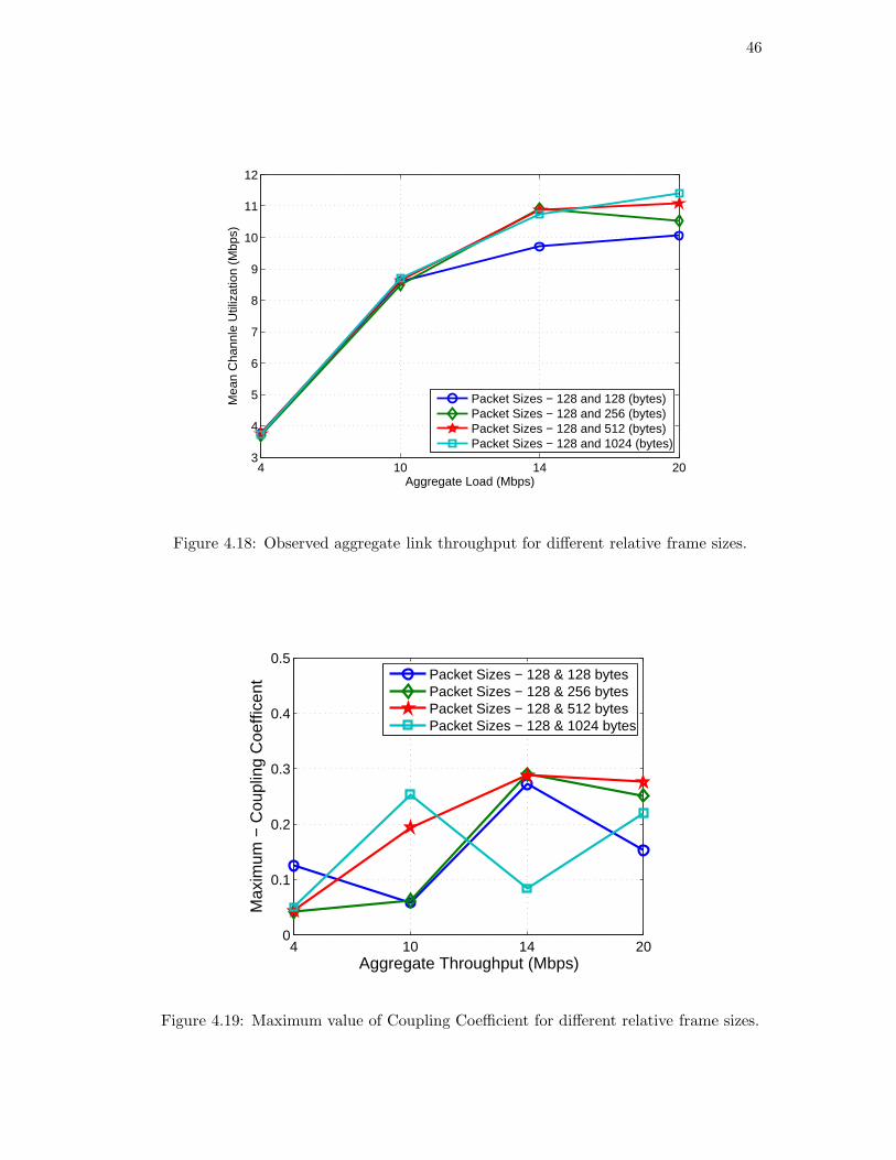
46
4 10 14 203
4
5
6
7
8
9
10
11
12
Aggregate Load (Mbps)
Mea
n C
hann
le U
tiliz
atio
n (M
bps)
Packet Sizes − 128 and 128 (bytes)Packet Sizes − 128 and 256 (bytes)Packet Sizes − 128 and 512 (bytes)Packet Sizes − 128 and 1024 (bytes)
Figure 4.18: Observed aggregate link throughput for different relative frame sizes.
4 10 14 200
0.1
0.2
0.3
0.4
0.5
Aggregate Throughput (Mbps)
Max
imum
− C
oupl
ing
Coe
ffice
nt
Packet Sizes − 128 & 128 bytesPacket Sizes − 128 & 256 bytesPacket Sizes − 128 & 512 bytesPacket Sizes − 128 & 1024 bytes
Figure 4.19: Maximum value of Coupling Coefficient for different relative frame sizes.

47
4 10 14 200.5
0.55
0.6
0.65
0.7
0.75
0.8
0.85
0.9
0.95
1
Aggregate Load (Mbps)
Min
imum
− F
airn
ess
Inde
x
Resource Ratio − 1:1Resource Ratio − 1:2Resource Ratio − 1:5Resource Ratio − 1:10
Figure 4.20: Minimum value of Fairness Index for different slice weight ratios.
4 10 14 202
4
6
8
10
12
14
Aggregate Load (Mbps)
Agg
rega
te T
hrou
ghpu
t (M
bps)
Resource Ratio − 1:1Resource Ratio − 1:2Resource Ratio − 1:5Resource Ratio − 1:10
Figure 4.21: Observed aggregate link throughput for different slice weight ratios.
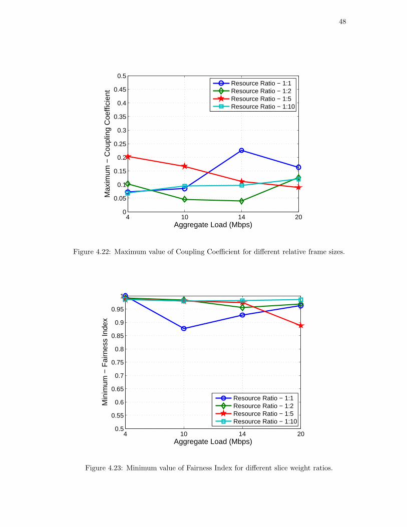
48
4 10 14 200
0.05
0.1
0.15
0.2
0.25
0.3
0.35
0.4
0.45
0.5
Aggregate Load (Mbps)
Max
imum
− C
oupl
ing
Coe
ffici
ent
Resource Ratio − 1:1Resource Ratio − 1:2Resource Ratio − 1:5Resource Ratio − 1:10
Figure 4.22: Maximum value of Coupling Coefficient for different relative frame sizes.
4 10 14 200.5
0.55
0.6
0.65
0.7
0.75
0.8
0.85
0.9
0.95
1
Aggregate Load (Mbps)
Min
imum
− F
airn
ess
Inde
x
Resource Ratio − 1:1Resource Ratio − 1:2Resource Ratio − 1:5Resource Ratio − 1:10
Figure 4.23: Minimum value of Fairness Index for different slice weight ratios.

49
4 10 14 202
4
6
8
10
12
14
Aggregate Load (Mbps)
Agg
rega
te T
hrou
ghpu
t (M
bps)
Resource Ratio − 1:1Resource Ratio − 1:2Resource Ratio − 1:5Resource Ratio − 1:10
Figure 4.24: Observed aggregate link throughput for different slice weight ratios.
4 10 14 200
0.05
0.1
0.15
0.2
0.25
0.3
0.35
0.4
0.45
0.5
Aggregate Load (Mbps)
Max
imum
− C
oupl
ing
Coe
ffici
ent
Resource Ratio − 1:1Resource Ratio − 1:2Resource Ratio − 1:5Resource Ratio − 1:10
Figure 4.25: Maximum value of Coupling Coefficient for different relative frame sizes.

50
Chapter 5
Conclusions and Future Work
This work proposes a technique to ensure fairness in Virtualized WiMAX scenarios.
A experimental deployment of a WiMAX BS is used to perform baseline performance
evaluation of this Base Station with multiple mobile end user WiMAX devices. This
provides a benchmark for the performance of the BS under different traffic loads and
channel conditions. We use this understanding of the practical limits of the base station
in terms of total network capacity, variations due to signal quality, etc.; to create virtual
slices of the WiMAX BS. This is done by creating virtual guests, using the Kernel Based
Virtual Machine (KVM) and mapping the slice flows to actual WiMAX service flows.
Further evaluation of the Virtualized Base Station indicates the potential for un-
fairness in channel access time of the slices in varying channel conditions. Maintaining
fairness between slices is an important requirement and to achieve this; we propose a
VNTS that uses a combination of scheduling and traffic shaping to provide the appro-
priate slice guarantees. We develop an algorithm, through which we query the BS, and
obtain a feedback of the current channel conditions for each MS. This information is then
used to determine the downlink data transfer rate that would ensure fairness amongst
slices. The downlink date rate for each slice is shaped dynamically, by VNTS Engine,
implanted using Click Modular Router. The VNTS Controller auto-reconfigures itself
and imposes fairness at preconfigured time intervals.
We perform experiments to observe a fairness index and channel utilization using
various schemes and use this data to select an optimal rate to shape at. Using these
rates, we perform experiments to observe the effectiveness of the VNTS technique under
different traffic types and varying loads. The results of these experiments indicate that
the proposed technique works well with various usage scenarios considered. There

51
was a significant coupling observed between the performance of clients under different
channel conditions, and the proposed scheme helps mitigate this effect; while ensuring
reasonable channel utilization.
Though the VNTS mechanism is efficient in enforcing policies under a wide range
of network conditions. Absence of control metrics makes it difficult to ensure fairness
in an efficient manner under certain situations. Assume a situation where VNTS is
managing two slices A and B with current slice utilization of 25% and 75% while their
desired allocation is 75% and 25% respectively. In such a case as long as the channel
is not saturated (total resource utilization is below 100%), we would not like to impose
any throughput restriction. In case we reach saturation, we would like to ideally like
to reduce the utilization of the offending slice B (since it is not supposed to use 75%)
a little so that the system stays below saturation instead of pruning slice B to 25% at
once. Such a mechanism will ensure fairness while allowing better channel utilization.
The VNTS mechanism does not allow such anadaptive enforcement for the lack of
efficient tools to determine current flow performance per slice (either in resource blocks
at the BS or end to end throughput).
Further work needs to be done to implement a scenario, where the VNTS technique
can be extended for each slice using multiple mobile clients at the same time. The
VNTS Engine should provide for dynamically adding processing blocks, as there are
new clients mapped to a particular slice. Click provides a technique called hotswapping
for this. A mechanism needs to be developed, through which the Click configuration
script can be generated and swapped on the fly.
The current VNTS technique needs to be further tested with a mobile user,in a real
deployment scenario; with varying channel conditions. The results that are obtained
with this deployment can provide a valuable feedback needed for fine tuning the system
to cope in all scenarios.

52
Appendix A
Implementation of VNTS Engine in Click
The VNTS Engine is implemented using Click Modular Router [27] In order to un-
derstand the working of the VNTS Engine, a basic understanding of Click terminology
and functions is essential.
A.1 Click Overview
The Click Modular Router was proposed by Eddie Kohler in his Ph.D. thesis [29]. Click
provides a software framework for building completely flexible and configurable software
routers. The basic building block of a Click router is an ”element”. An element can
be thought of as a node in a graph, where the packets flow from one element to the
other along the edges of the graph. This representation of router as a series of packet
manipulations provides an easy visualization of different router functions and makes
the router easily reconfigurable.
Each element is implemented as a C++ object and a connection is a pointer to this
object. Passing a packet along a connection in Click has the overhead of a single virtual
method invocation [27]. Click can run as a kernel module or as a user level tool.
Now we explain some of the terms and techniques used in the implementation of
Click Modular Router-
1. Element
An element is a module to process and manipulate packets in a router. It is possi-
ble for an element to have multiple input and output ports. Passing a packet from
the input port to the right port, after performing some function on it, comprised
the processing of a packet in an element. Each element has a configuration string;

53
and this serves as a parameter to change the behavior of that particular element.
There is an exhaustive list of elements that is already present and can be readily
used within a configuration file. The authors also provide the ability to create
and use one’s own element to perform specific user defined functions.
Figure A.1 illustrates a simple IP classifier element. This element has one input
port, which is the point of entry for packets entering this element. The element
class for this is ”IP Classifier” and the configuration string specifies IP address
on the basis of which the classification of packets needs to be done, and if the
IP address in question is the source IP address or the destination IP address.
This element has 2 output ports. The packets that are destined for the given IP
address are sent on output 1 and the rest of the packets are sent out on output 2.
IPClassifier(192.166.1.10, -)
Figure A.1: A Simple IPClassifier Element
2. Packet
A packet is a stream of bytes that are sent through the router. Click provides the
ability to generate these packets through elements like ”InfiniteSource” etc. One
also has the option to inspect, strip and mark particular bytes within the packet.
This facility allows us to annotate certain type of packets, and process them at a
later point of time, within the configuration.
3. Connections
In order to create a complete router, multiple click elements need to be connected
to each other. Click provides for connections through ports. The ports in an
element can be any one of the following three types-
(a) Push Port- Packets are pushed out on these ports. The connected element
does not need to request for the packet to be delivered to it. This is good
for arrivals and events in general.

54
(b) Pull Port- Packets need to be pulled out from these ports. The connected
downstream elements needs to ask for the packets, and only then the packets
are sent out. This type of port is good for polling and scheduling.
(c) Agnostic Port- This port can either be a push port or a pull port.
The connections of the elements need to be done in such a way that a push output
port is connected to a push input port and the same hold for pull. There can
be occasions where it might be necessary to convert a push to pull or a pull to
push. Click provides elements like Queue and Unqueue which can be used for
these operations.
4. Element Handlers
Click also provides the facility to actively read or write configuration strings for
the various elements, using element handlers. The Click element documentation
specifies if a handle is present for that particular element and also the type of han-
dle that is available. It is possible to open a control socket for a Click configuration
in user level, to address the element handler for an element. The control socket
can listen on a TCP port or a UNIX domain socket. Through this, Click listens
for commands that are sent it. This makes it convenient to change configurations
of routers, while it is being executed.
Sometimes it might be necessary to add new elements to click configurations,
while it is being executed. This can be done using Hot swapping. This refers
to changing the Click router configuration completely. When specified with the
right option, Click provides a writable hotconfig handler, which can be used to
accomplish the above mentioned task.
5. Example Configuration
We can now look at a simple example and see the various terms explained above,
in an actual click configuration.
Figure A.2 specifies a simple Click configuration, in which the packets are read
from the given interface (eth1 in our case), and are forwarded to a Classifier. The

55
FromDevice(eth1)
Classifier(12,0800 , 12/0806, -)
Print(ARP Packets) Print(IP Packets) Print(Rest)
ToDevice(eth1)
Figure A.2: Click example configuration
FromDevice element that reads the packets and sends them out is an example of
push processing. The Classifier element has a single input and 3 outputs. Packets
are classified into ARP Packets, IP Packets and Rest. The 12 in the Classifier
specifies the offset at which the Classifier searches for a matching entry. 0800 at
offset 12 signifies IP packets and 0806 at offset 12 specifies ARP packets. The -
specifies that any packets that do not match the above criteria are forwarded to
this port. Packets from this element are forwarded to a 3 different Print elements.
These element prints the packet to display, along with the specified label. From
here, the packets are forwarded to a common queue, which stores all the packets,
before returning them to the original interface using a ToDevice.
A.2 VNTS Engine Configuration
The control parameter for the Virtual Network Traffic Shaper (VNTS) is downlink
throughput and to manipulate downlink throughput rates, for each flow; in order to

56
ensure fairness of channel access time; we choose to use Click Modular Router. As
explained earlier, Click provides a modular form of implementing a software router.
Our Primary requirement here is to listen for any packets that come from the KVM
guest; and are headed for one of the WiMAX Clients, process those packets and send
them back to the original interface.
Any packet that is destined for any Client, and is originating from a KVM guest,
needs to pass through the external host machine, which forwards it to the ASN-GW,
which intern forwards it to the BS; through which it reaches the Client eventually.
Considering the given scenario, all the packets pass through eth1 interface on the Host
Machine and this is where I decide to capture the packets to process.
1. Design Overview
One of the primary differences of running Click in User Mode, as opposed to
Kernel Mode; is that, by using the FromDevice element, only a copy of the packets
is forwarded for processing and the original packets go through anyways. Hence,
any processing that might be done on these packets will not be reflected on the
network. A work around for this is to use the FromHost element.
The FromHost element captures any packets originating from the Linux Kernel
and pushes them on output 0. This element creates a tunnel device, which we
call fake0. This interface routes packets that are meant for the real Ethernet
device via FromHost, providing us with the required packets, that we can process
according to our requirements and forward it to the real Ethernet device using
the ToDevice element; from which they get forwarded to their destination.
A similar mechanism is provided for incoming packets via the element ToHost.
Here packets are read from the real Ethernet device using the FromDevice element.
These packets are then processed and the headers are changes accordingly, after
which they are forwarded to the ordinary Linux protocol stack.
The ”‘fake”’ device emulates all the properties of a real Ethernet device, while
providing us access to the original packets that are originating from and headed
back to the Linux kernel. The fake device can have the same or a different IP

57
address as the real Ethernet device. If it uses a different IP address then the
packet header needs to be changed such that outgoing packets appear as if they
are originating from the real device and also the incoming packets destination
needs to be changed to the fake device, before we return the packets to the Linux
kernel. The MAC header for the fake device can either be specified by the user
or a default value is chosen automatically.
The Click configuration can be divided into three parts, the Input Area, the
Processing Area and the Output Area. In the following three subsections, we
examine each part in greater detail.
2. The Input Area
FromDevce(eth1) FromHost(fake)
CheckIPHeader(14)
Classifier(12,0806 20/001, 12/0806 20/002, 12/0800)Classifier(12,0800 , 12/0806, -)
Tee ARPResponder(0/0 1:1:1:1:1:1) Strip(14)
Output Area
ARPQuerier(eth1)
Processing Area
Figure A.3: VNTS Engine input area
The input area,as shown in figure A.3 can be further divided into two parts -
packets that enter from the Internet, through the FromDevice; and packets that
are pulled from the Kernel, via FromHost. Packets entering from the FromHost
device are put through a classifier; which separates the IP packets, ARP Queries
and ARP replies. The ARP replies that are seen here are usually in response
to the queries that are sent by external devices and are directly forwarded to
the ToDevice. The ARP requests that are coming in on this device are sent by

58
the kernel and we respond to these queries using a fake responder that forces
the kernel to give us frames with 1:1:1:1:1:1 destination and 0:1:2:3:4:5 source
(default for fake0 device). The rest of the packets are IP packets and these have
the MAC header which contains all the fake data. This needs to be stripped.
After stripping this; the packets are forwarded for further processing.
The packets that are coming in through the FromDevice are also classified using a
Classifier to separate out the ARP packets from the IP packets. The ARP packets
(requests and replies) are duplicated using a Tee element and one copy is sent to
the ARP Querier that is waiting for the replies to come if from the internet for the
device it needs to forward to and the other copy to the host. The IP Packets that
come in are out through a basic CheckIPHeader element to validate the packets,
and then forwarded for further processing.
3. The Processing Area
MarkIPHeader(14)
IPClassifier(src net fake, -)
StoreIPHeader(14)
FixChecksums
Input Area 1
Strip(14)
StoreIPAddress(fake)
FixChecksums
SetIPAddress(next hop)
ArpQuerier(eth1)
IPClassifier(dst 1P, dst 2 IP , -)
BandwidthRatedSplitter(dst 1 rate) BandwidthRatedSplitter(dst 1 rate)
Discard Discard
Input Area 2
Output Area
Figure A.4: VNTS Engine processing area

59
The packets that enter the router are Classified at the Input area are then for-
warded to the Processing Area(figure A.4, if they need further processing. This is
where we do the meat of the work in the router. As before, there are two streams
of packets that are to be processed; one originating from the Kernel and the other
destined for the Kernel.
The packets that are coming from the Kernel are downlink packets in our scenario
and this is where we need to do the required shaping. The packets, after being
stripped of the fake MAC header need to store the real Ethernet header as the
source address and this is done using the StoreIPAddress element. These packets
now need to be checked if the checksum of these packets is as intended. For this,
I write an element that classifies the packets according to the type of data that
they contain and fixes the checksum accordingly. Now, we need to find out how
to get to the destination address and for this ARP Query needs to be sent to the
destination. This is done using the element ”ARPQuerier”. Packets arriving on
input 0 of the ARPQuerier need to be IP packets with their annotation set. If an
Ethernet address is already known for the destination, the IP packet is wrapped
in an Ethernet header and sent to output 0. Otherwise the IP packet is saved
and an ARP query is sent instead. If an ARP response arrives on input 1 for an
IP address that we need, the mapping is recorded and any saved IP packets are
sent.
The Packets from here are forwarded to an IPClassifier. Here, we classify pack-
ets based on the destination IP address. Since we have a one to one mapping
from a virtual container to a WiMAX Client, shaping traffic destined for the
client is equivalent to shaping traffic from the Virtual Machine. Packets meant
for each client are sent to an individual processing area.This area comprises of a
BandwidthRatedSplitter and sink to discard the unwanted packets. The Band-
withRatedSplitter is the main control factor for the packets that we capture.
This element splits the packets into two streams. The configuration string spec-
ifies the maximum rate that the packets can be given out on output 0. This
output 0 provides the packets at the rate which we desire. The remaining packets
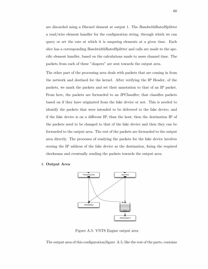
60
are discarded using a Discard element at output 1. The BandwithRatedSplitter
a read/wire element handler for the configuration string, through which we can
query or set the rate at which it is unqueing elements at a given time. Each
slice has a corresponding BandwidthRatedSplitter and calls are made to the spe-
cific element handler, based on the calculations made to asses channel time. The
packets from each of these ”shapers” are sent towards the output area.
The other part of the processing area deals with packets that are coming in from
the network and destined for the kernel. After verifying the IP Header, of the
packets, we mark the packets and set their annotation to that of an IP packet.
From here, the packets are forwarded to an IPClassifier, that classifies packets
based on if they have originated from the fake device or not. This is needed to
identify the packets that were intended to be delivered to the fake device; and
if the fake device is on a different IP, than the host; then the destination IP of
the packets need to be changed to that of the fake device and then they can be
forwarded to the output area. The rest of the packets are forwarded to the output
area directly. The processes of readying the packets for the fake device involves
storing the IP address of the fake device as the destination, fixing the required
checksums and eventually sending the packets towards the output area.
4. Output Area
ToDevice(eth1)
ToHost(fake)
Processing Area Input Area
Figure A.5: VNTS Engine output area
The output area of this configuration(figure A.5, like the rest of the parts; contains

61
two parts. The ToDevice output that is used to send packets out on the network
and the ToHost output that is used to send packets to the Kernel. The IP packets
that are originating from the kernel, after being shaped, need to be sent out. Since
there are multiple processing parts that try to send packets out to the real device,
the real device needs to be preceded by a queue. This queue ensures that the
packets are lined up and that the real Ethernet device can take the packets at a
rate that is best suited to it. The ToHost part of the output area forwards packets
to the Kernel and therefore, even if there are multiple processes that are sending
packets to the host, a queue element need not be present; since the Kernel can
take packets at any rate.
FromDevice(eth1) FromHost(fake)
CheckIPHeader(14)
MarkIPHeader(14)
IPClassifier(src net fake, -)
StoreIPHeader(14)
Classifier(12,0800, 12/0806 20/002, 12/0806 20/001)Classifier(12,0800 , 12/0806, -)
Tee ARPResponder(0/0 1:1:1:1:1:1) Strip(14)
StoreIPAddress(fake)
FixChecksums
SetIPAddress(next hop)
ToDevice(eth1)
ArpQuerier(eth1)
IPClassifier(dst 1P, dst 2 IP , -)
BandwidthRatedSplitter(dst 1 rate) BandwidthRatedSplitter(dst 1 rate)
FixChecksums
ToHost(fake)
Discard Discard
Figure A.6: VNTS Engine configuration diagram
5. Challenges Faced

62
The main challenge with using click in User mode is that by using a simple
FromDevice element, we do not get access to the Kernel packets. This is done
using FromHost. The FromHost element requires one to specify all the aspects of
routing, including handling ARP requests and responses. This needs to be config-
ured carefully, to ensure that the right device gets the ARP query/response. The
shaping aspect of this configuration was initially implemented using the Band-
widthRatedUnqueue element. It was observed that this element had a tendency
to hog CPU utlisation, as soon as it was required to pull packets from a queue at
a specified rate. A work around this problem was found by the use of the Band-
widthRatedSplitter element. The unwanted packets were discarded explicitly;
and this resulted in the CPU utlisation being restored to normal.

63
References
[1] Meilong Jang. NEC WiMax Base Station Document.
[2] M. Tim Jones. Virtual Linux - An overview of virtualization methods, architec-tures, and implementations. http://www.ibm.com/developerworks/library/
l-linuxvirt/index.html.
[3] D. Raychaudhuri, M. Ott, and I. Secker. Orbit radio grid tested for evaluation ofnext-generation wireless network protocols. In TRIDENTCOM ’05: Proceedingsof the First International Conference on Testbeds and Research Infrastructures forthe DEvelopment of NeTworks and COMmunities, pages 308–309, Washington,DC, USA, 2005. IEEE Computer Society.
[4] Hamed Soroush, Nilanjan Banerjee, Aruna Balasubramanian, Mark D. Corner,Brian Neil Levine, and Brian Lynn. DOME: A Diverse Outdoor Mobile Testbed. InProc. ACM Intl. Workshop on Hot Topics of Planet-Scale Mobility Measurements(HotPlanet), June 2009.
[5] E. Ertin, A. Arora, R. Ramnath, M. Nesterenko, V. Naik, S. Bapat, V. Kulathu-mani, M. Sridharan, H. Zhang, and H. Cao. Kansei: a testbed for sensing atscale. In Information Processing in Sensor Networks, 2006. IPSN 2006. The FifthInternational Conference on, pages 399–406, 0-0 2006.
[6] GENI. http://www.geni.net/.
[7] VINI. http://www.vini-veritas.net/.
[8] Alexander Sayenko, Olli Alanen, Juha Karhula, and Timo Hamalainen. Ensuringthe qos requirements in 802.16 scheduling. In MSWiM ’06: Proceedings of the 9thACM international symposium on Modeling analysis and simulation of wirelessand mobile systems, pages 108–117, New York, NY, USA, 2006. ACM.
[9] J. Lakkakorpi, A. Sayenko, and J. Moilanen. Comparison of different schedulingalgorithms for wimax base station: Deficit round-robin vs. proportional fair vs.weighted deficit round-robin. In Wireless Communications and Networking Con-ference, 2008. WCNC 2008. IEEE, pages 1991–1996, 31 2008-April 3 2008.
[10] J. Sun, Yanling Yao, and Hongfei Zhu. Quality of service scheduling for 802.16broadband wireless access systems. In Vehicular Technology Conference, 2006.VTC 2006-Spring. IEEE 63rd, volume 3, pages 1221–1225, May 2006.
[11] Yi-Neng Lin, Che-Wen Wu, Ying-Dar Lin, and Yuan-Cheng Lai. A latency andmodulation aware bandwidth allocation algorithm for wimax base stations. InWireless Communications and Networking Conference, 2008. WCNC 2008. IEEE,pages 1408–1413, 31 2008-April 3 2008.

64
[12] Jin-Cherng Lin, Chun-Lun Chou, and Cheng-Hsiung Liu. Performance evaluationfor scheduling algorithms in wimax network. In Advanced Information Networkingand Applications - Workshops, 2008. AINAW 2008. 22nd International Conferenceon, pages 68–74, March 2008.
[13] Chakchai So-In, R. Jain, and A.-K. Tamimi. Scheduling in ieee 802.16e mobilewimax networks: key issues and a survey. Selected Areas in Communications,IEEE Journal on, 27(2):156–171, February 2009.
[14] Sheng-Tzong Cheng, Bo-Fu Chen, and Chih-Lun Chou. Fairness-based schedulingalgorithm for tdd mode ieee 802.16 broadband wireless access systems. In Asia-Pacific Services Computing Conference, 2008. APSCC ’08. IEEE, pages 931–936,Dec. 2008.
[15] Fen Hou, J. She, Pin-Han Ho, and Xuemin Shen. Performance analysis of weightedproportional fairness scheduling in ieee 802.16 networks. In Communications, 2008.ICC ’08. IEEE International Conference on, pages 3452–3456, May 2008.
[16] Godfrey Tan and John Guttag. Time-based fairness improves performance inmulti-rate WLANs. In Proceedings of the 2004 USENIX Technical Conference.USENIX Association, June 2004.
[17] Ieee standard for local and metropolitan area networks part 16: Air interface forfixed and mobile broadband wireless access systems amendment 2: Physical andmedium access control layers for combined fixed and mobile operation in licensedbands and corrigendum 1. Technical report, 2006.
[18] J. G. Andrews, Arunabha Ghosh, and Rias Muhamed. Fundamentals of WiMAX-Understanding Broadband Wireless Networking. Prentice Hall, 2007.
[19] Dr. Sassan Ahmadi. Introduction to mobile WiMAX Radio Access Technology:PHY and MAC Architecture. http://www.mat.ucsb.edu/~ggroup/ahmadiUCSB_slides_Dec7.pdf.
[20] Yan Zhang and Hsiao-Hwa Chen. MOBILE WiMAX - Toward Broadband WirelessMetropolitan Area Networks. Auerbach Publications, 2007.
[21] Fan Wang, A. Ghosh, C. Sankaran, P. Fleming, F. Hsieh, and S. Benes. Mobilewimax systems: performance and evolution. Communications Magazine, IEEE,46(10):41–49, October 2008.
[22] D. Triantafyllopoulou, N. Passas, A.K. Salkintzis, and A. Kaloxylos. A heuristiccross-layer mechanism for real-time traffic in ieee 802.16 networks. In Personal,Indoor and Mobile Radio Communications, 2007. PIMRC 2007. IEEE 18th Inter-national Symposium on, pages 1–5, Sept. 2007.
[23] A.E. Xhafa, S. Kangude, and Xiaolin Lu. Mac performance of ieee 802.16e. In Ve-hicular Technology Conference, 2005. VTC-2005-Fall. 2005 IEEE 62nd, volume 1,pages 685–689, Sept. 2005.
[24] An Introduction to Virtualization. http://www.kernelthread.com/
publications/virtualization/.

65
[25] M. Tim Jones. Discover the Linux Kernel Virtual Machine- Learn the KVMarchitecture and advantages . http://www.ibm.com/developerworks/linux/
library/l-linux-kvm/resources.
[26] Kvm: Kernel-based virtualization driver. White Papper.
[27] Robert Morris, Eddie Kohler, John Jannotti, and M. Frans Kaashoek. The clickmodular router. In SOSP ’99: Proceedings of the seventeenth ACM symposium onOperating systems principles, pages 217–231, New York, NY, USA, 1999. ACM.
[28] Rajendra K. Jain, Dah-Ming W. Chiu, and William R. Hawe. A quantitativemeasure of fairness and discrimination for resource allocation in shared computersystems. Technical report, Digital Equipment Corporation, September 1984.
[29] Eddie Kohler. The Click Modular Router. PhD thesis, Massachusetts Institute ofTechnology, 2001.
Top Related