


Languages
Pages
Legal

NASA Technical Memorandum 102802
Velocity Filtering Applied toOptical Flow CalculationsYair Barniv
August1990
(NASA-TM-IOFSn2) VFLOCITY FILTERING APPLIEr_Tn O_:TICAL FLO_w CALCULATIONS (NASA) _8 r)
CSCL 2OD
,_;}/04
Nq0-ZF_)IZ
Oncl_s
0305027
NationalAeronauticsandSpaceAdministration
https://ntrs.nasa.gov/search.jsp?R=19900019196 2018-07-24T03:18:56+00:00Z

NASA Technical Memorandum 102802
Velocity Filtering Applied toOptical Flow CalculationsYaJr Bamiv, Ames Research Center, Moffett Field, California
August 1990
NationalAeronauticsanclSpace Aclminis_ation
Anms Research CenterMoffett F_lcl. Cal'domia94035-1000

CONTENTS
ABBREVIATIONS .......................................................................... v
1 INTRODUCTION ......................................................................... 1
2 PRELIMINARIES ......................................................................... 2
2.1 Motion as Tnne-Augmentcd Space .....................................................2
2.2 The Dirac Delta Function ..............................................................3
2.3 3-D FourierTransform of a Moving Point...............................................3
2.4 3-D FourierTransform of a Moving 2-D Line ...........................................5
2.5 3-D FourierTransform of a Moving Wave ..............................................7
2.6 Discussion of References ..............................................................9
3 3-D FOURIER TRANSFORM OF A FINITE-TIME MOVING POINT ..................... 10
4 MATCHED FILTERING APPLIED TO A MOVING POINT ............................... 10
4.1 Matched Filtering in the Fomicr Transform Domain .................................... 11
4.2 Matched Filtering in thc Spatiagrcmporal Domain ..................................... 12
5 IMPLEMENTATION OF THE MATCHED FILTER ....................................... 13
6 VELOCITY RESOLUTION OF A 3-D MATCHED FILTER ...............................14
6.1 General Derivation...................................................................14
6.2 Rcquircd Number of VelocityF'fltcrs..................................................18
6.3 Velocity Filter Algorithm ............................................................. 20
6.4 Computational Load and Mcmm'y Requirement ........................................ 21
7 APPLICATION TO THE OPTICAL HOW PROBLEM ................................... 22
7.1 General .............................................................................. 22
7.2 Why Constant-Speed Filters Cannot Work ............................................. 23
7.3 Using Velocity Profile Filters .......................................................... 25
ALGORITHM IMPLEMENTATION ...................................................... 33
8.1 Main Routines ....................................................................... 33
8.2 Preprocessing ........................................................................ 34
8.30bject's Expansion Between Frames .................................................. 35
8.4 Methods of Interpolation .............................................................. 36
8.5 The Algorithm Parameters ....................................................... • .... 37
..°
111

8.6 Data Sets Used ....................................................................... 38
8.7 General Discussim and Summary ..................................................... 42
8.8 Future Work .......................................................................... 44
REFERENCES ............................................................................. 52
iv
CFAR
DF
FOE
FOV
FP
FT
HPF
LPF
MF
PSF
SNR
2-D
3-D
ABBREVIATIONS
constant false alarm rate
delta function
focus of expansion
field of view
floating point
Fourier transform
high-pass filtering
low-pass filtering
matched filter
point-spread function
signal-to-noise ratio
two-dimensional
three-dimensional
V

SUMMARY
Optical flow is a method by which a stream of two-dimensional images obtained from a passive sen-
sor is used to map the three-dimensional surroundings of a moving vehicle. The primary application of
the optical-flow method is in helicopter obstacle avoidance. Optical-flow calculations can be performed to
determine the 3-D location of some chosen objects, or, in principle, of all points in the field of view of the
moving sensor as long as its trajectory is known. Locating a few objects, rather than all three-dimensional
points, seems to require fewer calculations but it requires that the objects between successive frames be
identified.The applicationof velocityfilteringtothisproblem eliminatesthe need foridentificationalto-
getherbecause it automatically tracks all moving points based on the assumption of constant speed and
gray levelper point.Velocityfilteringisa track-before-detectmethod and, as such,itnot only tracksbut
alsointegrates the energy of each pixelduring the whole observationtime, thus enhancing the signal-to-
noise ratioof each trackedpixel.This method is,in addition,very efficientcomputationally because it
isnaturallyamenable toparallelprocessing.A substantialamount of engineeringand experimental work
has been done inthisfield,and the purpose here istoexpand on the theoreticalunderstanding and on the
performance analysisof the velocityfilteringmethod, as wellas topresentsome experimentalresults.
1 INTRODUCTION
Opticalflow isa method by which a stream of two-dimensional (2-D) images obtained from a pas-
sivesensor isused to map the three-dimensional(3-D) surroundingsof a moving vehicle.The primary
applicationof the optical-flowmethod isin helicopterobstacleavoidance. Optical-flowcalculationscan
be performed to determine the 3-D locationof some chosen objects(referredto as feature-based)or,in
principle,ofallpointsinthefieldof view (FOV) of themoving sensor(referredtoas pixel-based).In both
cases it is assumed that the flight trajectory is known. Locating a few objects rather than all 3-D points
seems torequirefewer calculations,but itdoes requirethatthe objectsbe identifiedbetween successive
frames. Inpixel-basedmethods thereis no need toidentifyobjects since every pixelis definedtoconstitute
an object,and itisrecognizableby its(assumed) constantgray leveland itsapproximate location.
Velocity filtering is a track-before-detect method; as such, it not only tracks but also integrates the
energy of each pixelduring the whole observationtime,thus enhancing the signal-to-noiseratio(SNR)
of each trackedpixel.This method is,in addition,very efficientcomputationally,because itisnaturally
amenable toparallelprocessing.Inthispaper we develop and apply thetheoryof velocityfilteringtopixcl-
based passiveranging via opticalflow.The basictheoryof thevelocityfilteras realizedin thefrequency
domain isgiven inreference1.Applicationof thismethcxl---stillinitsfrequency-domain interpretation--
totheunderstandingofhuman visualmotion sensingcan be found inreference2,and applicationtoobject
trackinginreferences3-5.The method of"vclocityfiltering"has been suggested asa pixel-bascdsolution
inreference6. More detailedcomments about thesereferenceswillbc presentedinthe next section.
The purpose of this paper is to provide some insight into the performance of the velocity-filtering
method as applied to optical flow in order to be able to answer such questions as the following.
1. What is the smallest object that can be detected, or, equivalently, what is the minimum required
contrast of a single pixel for reliable detection (velocity measurement) as a function of its image speed?
2. What is the required FOV to detect a Oven-size object at a given range and under given visibility
conditions(fog, rain, or haze)?
3. How many velocity fillers are required, and, as a result, what is the required computational through-
put and memory?
Toward that end, the following tasks, which, so far as I know are areas of original work, are addressed.
1. Derive and interpret the space-domain shift-and-add algorithm from the general 3-D matched-filter
formulation.
2. Develop a formulation for the velocity-passband of the filter and a method for covering a given 2-D
velocity domain with complementing filters.
3. Develop the velocity-profile (hyperbolic) filter for optical-flow use and calculate its depth passband
and accuracy.
4. Implement the optical-flow shift-and-add version of the velocity-profile filtering algorithm and
develop appropriate preprocessing and interpolation methods.
In terms of an overall sensor/computer system, there is always a variety of trade-offs available to the
system designer. For example, a very narrow FOV will enable the detection/wacking of small obstacles at
a long distance in fog, but it will also provide a very limited view of the world. In this work, some tools
are developed that can help the designer make these trade-offs.
Section 2 summarizes some of the basic concepts regarding the representation of moving objects in
time-augmented space and the interpretation of the resulting Fourier transforms fits). The FT of a finite-
time moving-point is given in section 3, its corresponding matched-filter (MF) is derived in section 4, and
the MF is implemented in section 5. Section 6 deals with the passband and resolution of the velocity filter.
In section 7 the general velocity filter formulation is applied to the optical-flow problem and is modified
to also apply in the case of non-constant object velocities. In section 8 the new algorithm is implemented,
and its performance on two real-imagery sets is discussed.
2 PRELIMINARIES
The basic concepts and mathematical tools that are applied in subsequent sections are presented here.
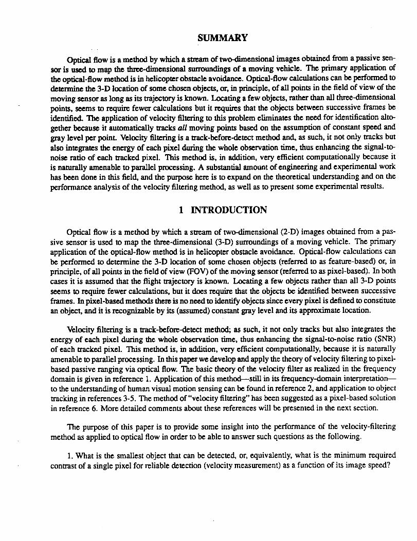
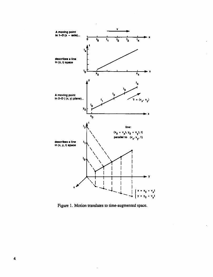
2.1 Motion as Time-Augmented Space
The motion of a physical point in one or two dimensions can be described as a line or a surface in a
space that is augmented by the time dimension. Let us start with the simplest example of a point moving at
some constant speed along the a-axis of a 1-D coordinate system. If the z-location and the corresponding
times for each value of z are listed, this relationship can be plotted as a straight line in a 2-D coordinate
system of (=, t). For a point that started from zo at to, and travels at a constant speed v, an equation of a
2
straightline is obtained: x = xo + v(t - %) as shown in figure 1. L If, instead of a constant speed, there
is a constant acceleration, a parabola in the (x, t) space would be obtained.
Figure 1 also shows an example of a constant-velocity point in the (x, F) plane that describes a straight
line in the 3-D space (x, _, t). This line can be given in two different forms; one is a parametric form in
which t serves as a parameter, that is, (x0 + vzt,_o + rut,t), and the other is as an intersection of two
planes: the plane parallel to the _-axis, x = x0 + vzt, and the plane parallel to the x-axis, _ = y0 + v_t. The
parametric form has the advantage that it can be easily related to the vector ( v_, vv, 1) which is parallel to
the line.
2.2 The Dirac Delta Function
The Dirac delta function z(t) = 6(0 can be defined as the limit when T ---, 0 of a rectangle pulse
function centered on t = 0 whose width is T and whose height is 1/T, or more generally by the properties
6(t)- O t_O (1)f_o t( t)d;t = I
The most important property of the delta function is its sifting property, that is,
f)5 6(t - _,)f(_,)ct>, f(t) (2)
One can similarly define a 2-D Dirac delta function such that its integral between 4-00 in 2-D equals
1, that is,
f f'_2 62(x'It)dxgV = 1 (3)
and it has the sifting property
f'_Sf_S =,,,,- = (4)
where the superscript 2 differentiates between the 1- and 2-D delta functions. From equation 2 we see that
82(x, V) can be replaced by 6(x)6(V) and still yield the same result, because the 2-D integral could then
be separated into two 1-D integrals. This is why, for all practical purposes, the following equality (see
ref. 7) can be used:
62(z, v) = 6(x)6(v) (5)
Another useful equality that can be proven by a simple change of variables is
62 (ax, by) = 1---1---62 (x, V) (6)la61
2.3 3-D Fourier Transform of a Moving Point
Earlier in this section, the trajectory or geometrical location of a point moving at a constant velocity
on the plane was discussed. Thus, there is a functional relationship between location and time of the form
A moving pointIn 1--D (x - axis)...
describes a linein (x, t) apace
A moving pointin 2-D ( (x, y) plane)...
describes a linein (x, y, t) space
| I I i / I _ xO tO tI t2 t3 t4 r
t t4_
to xX0 X4
0 y _ _t4_ v
X' Vy)t
Y
_XXo
t2!\\
tl'_
\\
\
line:
(x0 ÷ Vxt' Y0 + Vyt, t)
parallel to (vx, Vy, 1)
\ \
\\ \\ _'_
,o,\ \. Yi !
1" I I I ',
\ ; I I l I\_l I I I II
I
-- y
X = X0 + VxtY = YO + Vyt
Rgu_ 1. Motion translates to timc-augmcnr_lspace.
4
x(t), I/(0 • Here we want to refer to the amplitude of the point (in addition to its trajectory) which is a
function of location and time.
A point that moves on the (x, I/) plane with a fixed velocity vector _ - (vffi, W) can be described as
a moving 2-D delta function (DF), that is,
s( z,v,t) = 8( z - xo - v_t)6(I/- I/o - vvt)
= 62 (_ - _0 - _t) (7)
Notice that s was chosen to be the amplitude function of the moving point so that at any given time, its 2-D
integral over the (x, 1/) plane is unity. Also notice that, using _ _= (x, V), a new vectorial form for the 2-D
delta function, which is more convenient and concise to work with, has been defined through equation 7.
The 3-D Fourier wansform (FT) of s(x, 1/,t) is
=f f f exp{-jtot} exp(-jk. _} dt d_
= 21r exp{-jk • _0}SCw + k. _) (8)
where the vector k - (/¢,_,/%) is used to denote the spatial frequencies in radians per meter and the dot
product is used to denote scalar vector multiplication. The integrals in equation 8 and in all subsequent
equations are between the limits of 4-00 unless specified otherwise. The result in equation 8 is composed
of a phase term which depends only on the starting point _0 at t = 0, and on a 1-D delta function that can
be written in a more revealing form as
6( vzi¢_ + vvl % + to) (9)
To understand the meaning of a DF we equate its argument to zero, because, by definition, the DF is active
(goes to infinity) when its argument equals zero and it is zero elsewhere. Doing that results in
vsk, s + wkv + to= 0 (I0)
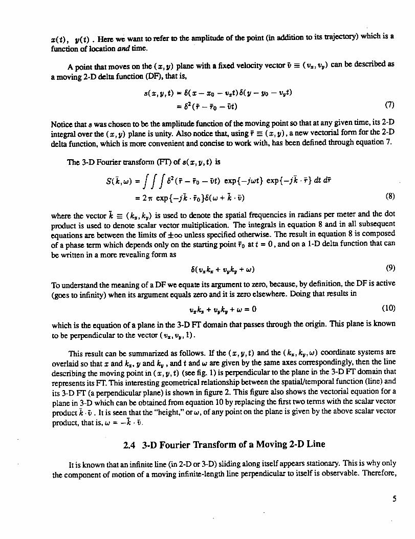
which istheequation of a plane inthe3-D FT domain thatpassesthrough the origin.This plane isknown
tobe perpendiculartothe vector(vz,v_,I).
This result can be summarized as follows. If the ( x, I/, t) and the (/¢_, k v, to) coordinate systems are
overlaid so that x and k,,, 1/and k v , and t and to are given by the same axes correspondingly, then the line
describing the moving point in (x, 1/, t) (see fig. 1) is perpendicular to the plane in the 3-D FT domain that
represents its FT. This interesting geometrical relationship between the spatial/temporal function (line) and
its 3-D FT (a perpendicular plane) is shown in figure 2. This figure also shows the vectorial equation for a
plane in 3-D which can be obtained from equation 10 by replacing the first two terms with the scalar vector
product k. _. It is seen that the "height," or to, of any point on the plane is given by the above scalar vector
product, that is, to -" -k • _.
2.4 3-D Fourier Transform of a Moving 2-D Line
It is known that an infinite line (in 2-D or 3-D) sliding along itself appears stationary. This is why only
the component of motion of a moving infinite-length line perpendicular to itself is observable. Therefore,
5
t'Ae) " _Theplane: v xk x + Vyky . m = 0
I _\ or: o):-k-.V
_perpendiculllr to original 3-D line
v_ Y, ky
/_ -(kx' kY' -_" V)
x, kx
Figure2. 3-D Fouriertransformof a moving point isa plane.
all velocity vectors of a moving infinite line that have the same component perpendicular to the line will
produce the same FT. As was shown for a moving point, the augmentation of the 2-D (x, V) plane to the
(a:, I/,t) volume makes the moving line in 2-D appear as a stationary plane in 3-D.
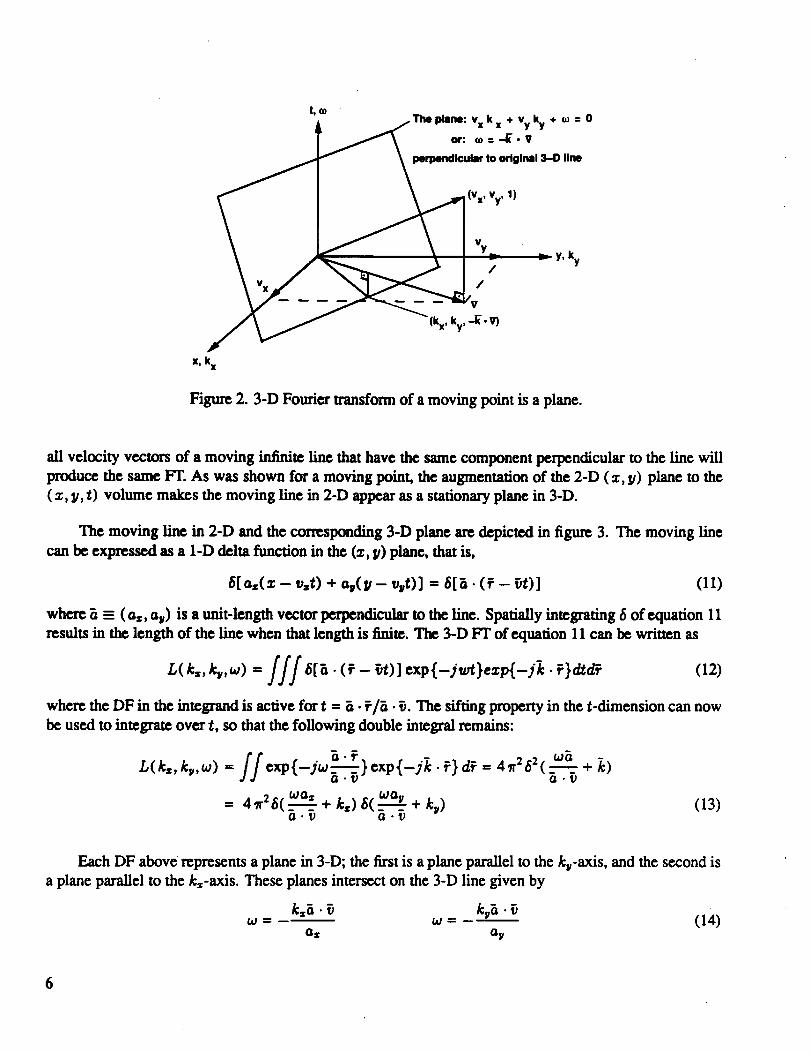
The moving line in 2-D and the corresponding 3-D plane are depicted in figure 3. The moving line
can be expressed as a 1-D delta function in the (=, It) plane, that is,
B[a.(= - _.t) + au(It - _ut)] -- B[fi-(_ - _,t)] (11)
where fi - (a,, a,,) is a unit-length vector perpendicular to the line. Spatially integrating 6 of equation 11
results in the length of the line when that length is finite. The 3-D FT of equation 11 can be written as
L( k,, k_,to) = f f f 6[_. (_ - _t)] exp{-j_vt)e:rp(-jk. _}_d_ (12)
where the DF inthe integrandisactivefort = _. _/_. _. The siftingpropertyin thet-dimension can now
be used tointegrateover t,so thatthe followingdouble integralremains:
m
H . O-I"L(k., ky,w) exp{-ywfi---_ } exp{-ji • _} d_ = 41r262( wa= --+i)(I't)
= 41r26(_w-_a_*+ kz) B(_---r_+ kU)a .17 rt ._7
(13)
Each DF above represents a plane in 3-D; the first is a plane parallel to the k_-axis, and the second is
a plane parallel to the k=-axis. These planes intersect on the 3-D line given by
to = to = (14)(;= Ov
6
Y Vy _.
\ Vp
\_ 3
k t2
tI
t=O
X
_ _ Y
//
//
X
Moving line in 2-D Stationary plane in 3-D
axX + ayy-J.gt = 0
Figure 3. 3-D representation of a moving 2-D line.
and a possible vector parallel to the intersection line has the components (a:, %,-_ • _). The/z vectorshown in figure 3 is perpendicular to the advancing line, so that _. v = _. _p = I _ II Isince _ and _p are
parallel. Thus, it has been proven that the other component of _, perpendicular to _p, has no effect on the
resultant 3-D line in the FT domain. If the original moving-line equation is written as the plane in the 3-D
(x, I/, t) domain shown in figure 3, that is,
a=x+ l a II It = o (15)
it is noted that this plane is perpendicular to the line in the FT domain, given by equation 14, which rep-
resents its transform. RecalLing the result of the previous section, we notice the expected duality withthe result here; that is, a line in (x, I/,t) (which represents a moving point in 2-D) transforms into a per-pendicular plane in the 3-D FT domain, and a plane in (x, I/, t) (which represents a moving line in 2-D)
transforms into a perpendicular line in the 3-D FT domain.
2.5 3-D Fourier Transform of a Moving Wave
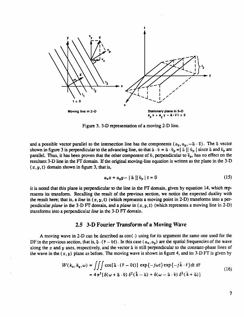
A moving wave in 2-D can be described as cos (.) using for its argument the same one used for the
DF in the previous section, that is, _. (7 - _t). In this case (a:, av) are the spatial frequencies of the wave
along the :r and I/axes, respectively, and the vector a is still perpendicular to the constant-phase lines of
the wave in the (:r, I/) plane as before. The moving wave is shown in figure 4, and its 3-D F'I" is given by
W( k,, k,,w) = f f f cos[_ . (_ - _t)] exp{-jtat} exp{-jk. _')dt dr.
= 4Ii'3[S(t0 + a. _) _2(k-- a) + _(w -- a. _) $2(_; + a)]
(16)
7
The 3-D FT of the moving 2-D wave consists of only two points, as shown in figure 4. These points are
anfisymmetric with respect to the origin and, thus, reside on a line that passes through the origin. All
waves having the same direction fi--irre_five of their frequency--yield two points on this line. The
speed of the wave (perpendicular to its fzont) determines the height of the two points above or below the
(ks, _) plane. In other words, when the speed is zero, the resulting two points in the 3-D FT domain
degenerate into the 2-D FT plane. It is the motion that raises the two points, or, for that matter, the 2-D FT
of any stationary 2-D pa#ern, into the w-dimension by slanting the zero-speed 2-D FT at an angle that is
proportional to the speed.
y
W(k x, ky, o)) = J']'_cos [ax (X-Vxt) ÷ ay (y - Vyt)] • exp {-j (tot ÷ k'. i_)} dTdt
= 4_318(0) + |.q) - 82(E- ii) , 8(o) - Z.V) • 82(E + |)]
= ]i'V i_ t0
_ ky
1
kx
01 -- --8*V
Figure 4. 3-D Fourier transform of a moving 2-D wave.
2.6 Discussion of References
Havingdevelopedthenecessarymathematicaltools,the references mentioned in the Introduction can
be discussed in more detail.
Reference 1: Reed et al. The concept of one-, two-, and three-dimensional Fourier transform is
well known (e.g., see ref. 8). Reed et al. seem to be the first to apply the 3-D matched filter to a moving
constant-velocity object-detection problem. In this paper, they develop the MF equations and the signal-to-
noise (SNR) expressions for the MF output. The complete development is done in the frequency domain,
although it is mentioned that alternative approaches can be used, such as "space-domain transversal filtering
schemes."
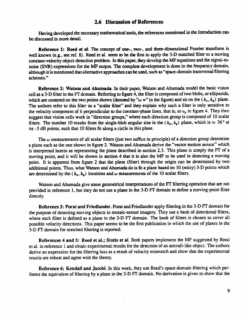
Reference 2: Watson and Ahumada. In their paper, Watson and Ahumada model the basic vision
cell as a 3-D filter in the FT domain. Referring to figure 4, the filter is composed of two blobs, or ellipsoids,
which are centered on the two points shown (denoted by "to =" in the figure) and sit on the ( kz, k_) plane.
The authors refer to this filter as a "scalar filter" and they explain why such a filter is only sensitive to
the velocity component of _ perpendicular to the constant-phase lines, that is, to v_, in figure 4. They then
suggest that vision cells work in "direction groups," where each direction group is composed of 10 scalar
filters. The number 10 results from the single-blob angular size in the (kz, k_,) plane, which is _ 36 ° at
its -3 dB points, such that 10 filters fit along a circle in this plane.
The w measurements of all scalar filters (just two suffice in principle) of a direction group determine
a plane such as the one shown in figure 2. Watson and Ahumada derive the "vector motion sensor" which
is interpreted herein as representing the plane described in section 2.3. This plane is simply the F'I" of a
moving point, and it will be shown in section 4 that it is also the MF to be used in detecting a moving
point. It is apparent from figure 2 that the plane (filter) through the origin can be determined by two
additional points. Thus, what Watson and Ahumada do is fit a plane based on 10 (noisy) 3-D points which
are determined by the ( kz, k_) locations and _o measurements of the 10 scalar filters.
Watson and Ahumada give some geometrical interpretations of the FT filtering operation that are not
provided in reference 1, but they do not use a plane in the 3-D FT domain to define a moving-point filter
directly.
Reference 3: Porat and Friedlander. Porat and Friedlander apply filtering in the 3-D FT domain for
the purpose of detecting moving objects in mosaic-sensor imagery. They use a bank of directional filters,
where each filter is defined as a plane in the 3-D FT domain. The bank of filters is chosen to cover all
possible velocity directions. This paper seems to be the first publication in which the use of planes in the
3-D FT domain for matched filtering is reported.
References 4 and 5: Reed et al.; Stotts et al. Both papers implement the MF suggested by Reed
et al. in reference 1 and obtain experimental results for the detection of an aircraft-like object. The authors
derive an expression for the filtering loss as a result of velocity mismatch and show that the experimental
results are robust and agree with the theory.
Reference 6: Kendall and Jacobi. In this work, they use Reed's space-domain filtering which per-
forms the equivalent of filtering by a plane in the 3-D FT domain. No derivation is given to show that the
9
two areequivalentandthattheyrepresentmatchedfilteringfor the case in which the imagery is corrupted
by while additive noise. This method yielded some preliminary results when implemented in a single
spatial dimension and appfied to two imagery sets.
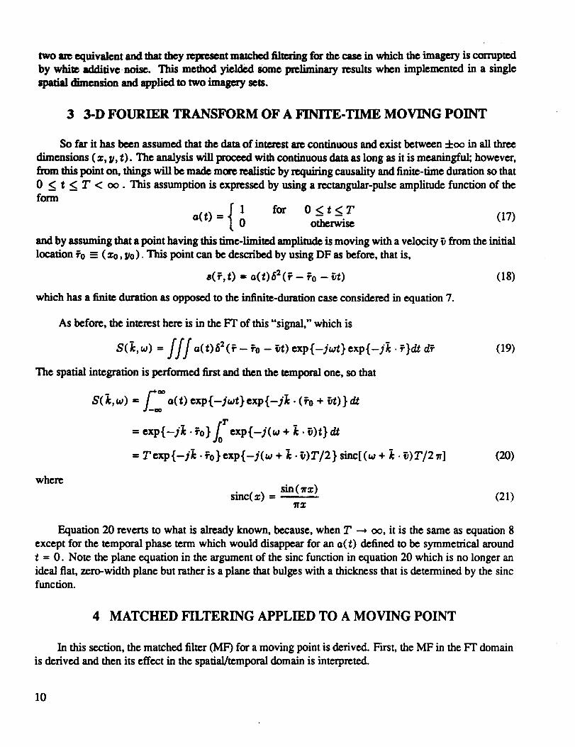
3 3-D FOURIER TRANSFORM OF A FINITE-TIME MOVING POINT
So far it has been assumed that the data of interest are continuous and exist between 4-00 in all three
dimensions (s, V, t). The analysis will proceed with continuous data as long as it is meaningful; however,
from this point on, things will be made more realistic by requiring causality and finite-time duration so that
0 < t __ T < oo. This assumption is expressed by using a rectangular-pulse amplitude function of the
form
1 for 0 <t<Ta(t) = 0 otherwise (17)
and by assuming that a point having this time-limited amplitude is moving with a velocity _ from the initial
location _o -- (s0, If0 ). This point can be described by using DF as before, that is,
s(Lt) = a(t)62(_ - _o - _t) (18)
which has a finite duration as opposed to the infinite-duration case considered in equation 7.
As before, the interest here is in the FT of this "signal," which is
=f f f o.)62( _ - exp{--jut} exp{-j_:. _}dt dr
The spatial integration is performed first and then the temporal one, so that
to) = ;ff a(t) exp {-jut} exp {-jk. (_0 + _t) }8( d,t
- exp{-/_. _o} exp{-j(to ÷ _. _)t}_
- r exp {-/_. _o}exp {-/( to ÷ i. _)7'/2 } sinc[(to + _. _)r/2 _1
(19)
(20)
wheresin(Its)
sinc(s) = (21)'R'X
Equation 20 reverts to what is already known, because, when T ---, oo, it is the same as equation 8
except for the temporal phase term which would disappear for an a(t) defined to be symmetrical around
t - 0. Note the plane equation in the argument of the sine function in equation 20 which is no longer an
ideal flat, zero-width plane but rather is a plane that bulges with a thickness that is determined by the sinefunction.
4 MATCHED FILTERING APPLIED TO A MOVING POINT
In this section, the matched filter (MF) for a moving point is derived. First, the MF in the FT domain
is derived and then its effect in the spatial/temporal domain is interpreted.
10
4.1 Matched Filtering in the Fourier Transform Domain
An MF is the filter that optimally enhances the signal's amplitude when it is embedded in white or
colored Gaussian noise. The well-known form of the MF for a signal embedded in white Gaussian noise
is (from refs. 9 and I0)
H(k,w) = S'(i,_a) exp{-jwT} (22)No
where No is the constant-spectrum value of the white noise, asterisk denotes complex conjugation, and the
output of the MP is wad out when it peaks at t = T. The temporal phase term makes sure that the filter is
reaflizable, so that its output is delayed until the end of the data stream. Passing the moving-point signal
(which generally also includes noise) through the MP of equation 22 amounts to taking the 3-D inverse
transform of the product,
G(k,w) = SClc,w)HCk,w) = T2sinc:[Cw + 7c.8)TI21t] exp{-jwT}INo (23)
which yields, by inverse FT transformation,
g(_,t) = (2,r)3N0 sinc2[.]exp{j[k._+_o(t-T)]}dkd_(24)
Substituting z = (w + k. _v)/2 7r,
r 2
t) = ( 2 ,r) 2 No f sinc2 (zT) exp {j2 ,rz(t - T) } ciz ff exp{jk • [ _ - _(t - T) ] } dkg(
= T/No 62[_ - _(t - T)] •ira(tiT) (25)
where tra(t/T) is the triangle function shown in figure 5. By definition, the output of an MF has to be
sampled at t = T to get the maximum output, or read-out of the last frame when the data are discrete in time.
At thatinstant,thereisa pointdetectionattheorigin,_ = 0, in the form of a 62(_) having an amplitude
proportionaltoT. The peak of the MF outputisattheoriginbecause spatiallynon-causalimages, which
existforbothpositiveand negativevaluesof_ components, arebeing used.Note, thatequation25 includes
thefactorT, so thattheresultof NIP operationislinearlyproportionaltotheobservationtime.
tral t/'t')
T 2Tt
Figure 5. Triangle function.
11
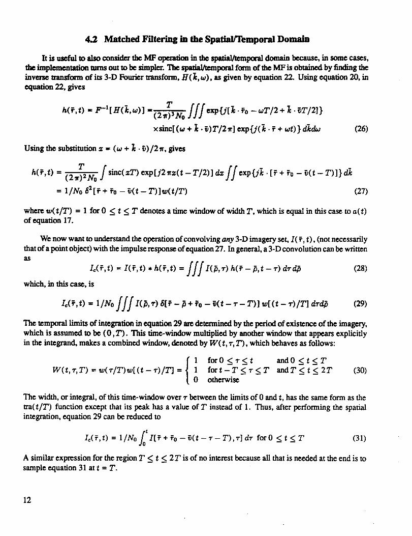
4.2 Matched Filtering in the Spatial/Temporal Domain
It is useful to also consider the MF operation in the spafiaYtemporal domain because, in some cases,the implementation turns out to be simpler. The spatiaFtemporal form of the MF is obtained by finding theinverse transfcmu of its 3-D Fourier transform, H(]:,w), as given by equation 22. Using equation 20, in
equation 22, gives
TJJJ exp{j[_. +0- a,T/2 + t. eT/2]}h(_',t) = F-l[ H( k,w) ] =(21r)3No
xsinc[(_ + [. _)T/2 It] exp{/(k. _ + wt)} dkdw (26)
Using the substimdon x : (w + ];. _)/2 _r, gives
h(f,t) = T f sinc(xT)exp[j2_rx(t-T/2)]d.x ff exp{j-k.[+++o-_(t-T)]}d_.(2_r)2N0
= l/N0 62[_ + r0 - _(t - T)]w(t/T) (27)
where w(t/T) : 1 for 0 < t < T denotes a time window of width T, which is equal in this case to a(t)of equation 17.
We now want to understand the operation of convolving any 3-D imagery set, I( +, t), (not necessarilythat of a point object) with the impulse response of equation 27. In general, a 3-D convolution can be writtenas
Ic(+,t) = I(+,t) • h(+,O = JJJl<_,r)h<+-_,t- r)arab, (28)which, in this case, is
ff/i< r)6[+- ++o- +.- r- T)]=[. - r)/r drd (29)Ic( t) 1/_v0
The temporal limits of integration in equation 29 are determined by the period of existence of the imagery,
which is assumed to be (0, T). This time-window multiplied by another window that appears explicitlyin the integrand, makes a combined window, denoted by W(t, "r,T), which behaves as follows:
1W(t, r, T) = w(r/T)w[ (t - T)/T] = 1
0
forO <T<t
fort-T <_r<_Totherwise
and0 <t<T
and T < t < 2 T (30)
The width, or integral, of this time-window over r between the limits of 0 and t, has the same form as the
tra(t/T) function except that its peak has a value of T instead of 1. Thus, after performing the spatialintegration, equation 29 can be reduced to
Ic(_,t) = 1�No I[++_o-_v(t-r-T),r]dr for0 < t < T (31)
A similar expression for the region T < t < 2 T is of no interest because all that is needed at the end is to
sample equation 31 at t = T.
12
To check the validity of the above general result, it is applied to the specific moving-point imagery of
equation 18, that is,
Ic(_,t) = 1�No a(r) 62[_+_o__(t_r_T) -% -_rldr
Z'= 1/1% _2[__ _(t- T)I gr
= t/No 62 [ _ - _(t - T) ] (32)
The interpretalion of equation 32 is the following. When discrete images are considered,/'c(_, t) represents
the whole imagery set so that Xc( _, 1) is the first frame and, say, Xc( _, 20) is the 20 t h frame of the convolved
imagery (after it has passed the MF). If we start with N original frames, we end up with 2 N frames out of
the MF. Since the MF is sampled at T, we are only interested in frame number N. It is seen that the results
of equations 32 and 25 agree at time t = T (frame number N), as expected.
$ IMPLEMENTATION OF THE MATCHED FILTER
To see what the operation of equation 31 means in terms of implementation, we rewrite it, sampled
art = T, that is, as
Ic(_, T) = 1/No I(_ + % + _', r) dr (33)
It is seen that the shifted versions of the original images have to be added (integrated), starting with the
first at 1"= 0, that is, I(_ + %, 0), and ending with the last at "r = T, that is, I( _ + % + _T, T). This means
that the last frame is shifted toward the origin by the vector _T relative to the first one. The additional shift
toward the origin of size _0, which is common to all frames, is a result of the particular MF being used,
which was matched to a point at _0. That shift would bring the point % to the origin. Since it is desired
to preserve the ori_nal location of any general point _0 in the resultant image, this point has to be shifted
back to where it came from. This can be accomplished by discarding the _0 term from equation 27. The
final effect would thus be that all points (pixels) after MF stay in the locations they had at t = 0 or at the
first frame of the original imagery.
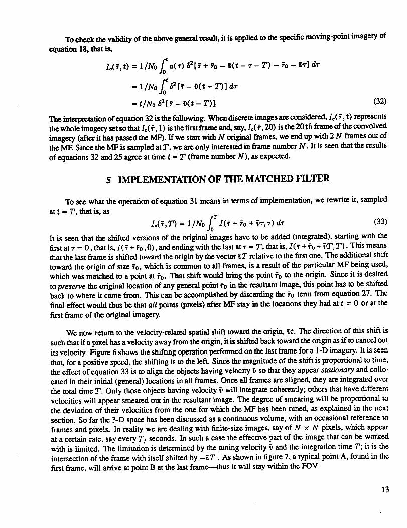
We now return to the velocity-related spatial shift toward the origin, _t. The direction of this shift is
such that if a pixel has a velocity away from the origin, it is shifted back toward the origin as ff to cancel out
its velocity. Figure 6 shows the shifting operation performed on the last frame for a 1-D imagery. It is seen
that, for a positive speed, the shifting is to the left. Since the magnitude of the shift is proportional to time,
the effect of equation 33 is to align the objects having velocity _ so that they appear stationary and collo-
cated in their initial (general) locations in all frames. Once all frames are aligned, they arc integrated over
the total time T. Only those objects having velocity _ will integrate coherently; others that have different
velocities will appear smeared out in the resultant image. The degree of smearing will be proportional to
the deviation of their velocities from the one for which the MF has been tuned, as explained in the next
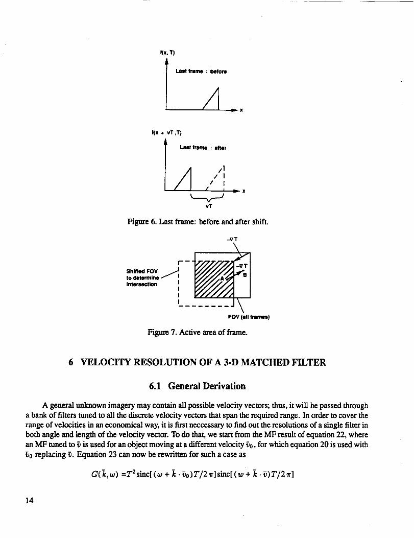
section. So far the 3-D space has been discussed as a continuous volume, with an occasional reference to
frames and pixels. In reality we are dealing with finite-size images, say of N x N pixels, which appear
at a certain rate, say every TI seconds. In such a case the effective part of the image that can be worked
with is limited. The limitation is determined by the tuning velocity _ and the integration time T; it is the
intersection of the frame with itself shifted by -_T. As shown in figure 7, a typical point A, found in the
first frame, will arrive at point B at the last frame---thus it will stay within the FOV.
13
l(x, I"9
Last tram : before
Av_ X
I(x + vT ,T)
TI
Last frame : alter
/_ /1/ I
/ I/
L-v-JvT
_-_ X
Figure 6. Last frame: before and after shift.
-qT
shm,eFov JJto determine ] !
intersection III
L
FOV (all frames)
Figm_ 7. Active area of frame.
6 VELOCITY RESOLUTION OF A 3-D MATCHED FILTER
6.1 General Derivation
A general unknown imagery may contain all possible velocity vectors; thus, it will be passed through
a bank of filters tuned to all the discrete velocity vectors that span the required range. In order to cover the
range of velocities in an economical way, it is first neccessary to find out the resolutions of a single filter in
both angle and length of the velocity vector. To do that, we start from the MF result of equation 22, where
an MF tuned to _ is used for an object moving at a different velocity _0, for which equation 20 is used with
_0 replacing _. Equation 23 can now be rewritten for such a case as
G(I¢,_) =Y2 sinc[ (_o + k. _o)T/2_r]sinc[(w + -k. %)T/2_r]
14
x cxp(j_,. A_T/2) exp (-jwT)/No (34)
where
The 3-D inverseFT, asinequation 24, sampled at t = T willbc
: I IIQ(_,T) = (21r)3No sine[ (w + k. _o)T/21r]sinc[(w + -k. _)T/2_r] d_
x exp[j_ .(_+ aZ,T/2)]
Using Parseval'stheorem, thatis,
and the FT pair,
/ f*(t)g(t)d_ = 2-_ J ]_(w)G(w)ako
w[(t + T/2)/T] exp(-jzt) _ Tsinc[ (w + z)T/2_r]
the first integral over w in equation 35 is replaced by
1---/Tsinc[.] Tsinc[.] c/_21r = fw[(t + T/2)/T]exp{flc ._ot}
• w[ (t + T/2)/T] exp(-jk. _t} dt
= [T/: exp(-jk. A_t} dt = Tsinc -(k • A_T_,-m \ ":-_ }
(35)
(36)
(37)
(38)
Now equation 35 roads
T ffsinc(_,.A_T_ exp{jk-(_ + A_T/2)} dk (39)g(_',T) = 41r:zNo _ "2-_ ]
We willskip somo simple but unwieldy derivation,and writethefinalmsuh as
g(_',T) = 1�No 6(Av=y - Avyz) , - TAv_ __ z < 0 (40)
which is a 2-D line DF on the bounded segment shown in figure 8. The total area under this segment is
L f tS(Av_y-Av, z) dxdy=T (41)Au_ TA_,
and itisdistributedevenly along it.Itisnoted thatthedimensions of6(Av_y - Avvx) are 6([m/sec][m])=
[sec]6([m:]), which isthe same as those of t_2(_) in equation 32, thatis,[sec]_([m])6([ra]) or
[ sec][m-:].
The line DF of equation 40 reduces to that of equation 32 evaluated at t = T when Av,, = 0 (which
implicitly also makes Avu = 0). The meaning of this result is that, because of the velocity mismatch, the
point detection of equation 32 smears over the length of the line segment of equation 40, which is
t= T_/a_ + a_ = T la_l (42)
15
¥
-T_v xI
Ja x
-T_Vy
Figure 8. Line-sesment delta function.
that is, the moving pixel is now detected in the form of a smeared ime segment rather than a single point
at the origin, as it was for A# = 0. This will cause location uncertainty along with a loss in gain.
Note that, because equation 42 depends on the absolute value of the speed mismatch, this equation
reveals the effect of both mismatch in speed and mismatch in the velocity-vector direction. For mismatch
in direction of size Aa,
Iavl= 2 Ivl sin(aa/2) (43)
Note too that it is the absolute value of the velocity vector mismatch that appears in the result of equation 42
and not the relative velocity vector mismatch.
The gain loss is simpler to understand when it is thought of in terms of discrete pixels rather than in
terms of continuous spatial distances. For I = p along, say, the z-axis (p denotes the side width of a pixel)
the peak smears over 2 pixels so that the loss is by a factor of 2 or-6 dB. Equation 42 can be rewritten for
the discrete case as
/p_ N [AVp[ (44)
where N is the total number of frames (replacing the integration time T ), and _p is the velocity measured
in pixels per frame. The expression of equation 44 is inaccurate for small [ A_ v [ values (of the order of
1/N pixelHrame) because of the pixels' discretization. However, we are particularly interested in such
small values because they correspond to losses of the order of-3 dB. We thus want to derive an accurate
expression for that range of interest as explained below.
Itisrealizedthatthe lossin gainresultsfrom smearing a l-pixelareaover more than a singlepixel.
Figure 9 shows a pixelthatissmear_ as a resultof shiftingitby (Az, AI/).For gain lossesof the order
of-3 dB, the peak of theMF outputwillstilloccur inthe nominal pixelthatisdenoted by (0,0).Thus, wc
want tofindthe intersectionareasbetween the shifted(smeared)pixeland the nominal pixclateach one
of theN frames and sum them up. When (Az, AV) = (0,0) thissum equalsN.
Counting frames from zero, that is, 0 < n < N - 1, the shift in pixel-width units at frame n is given
by
- n I I cos a, av ---n IAv,I sin _ (45)
The contribution that frame n makes to the nominal pixcl is (1 - nAz)(1 - nay) so that the loss (to. be
denoted by L,) can be written as the summation of the contributions of all N frames divided by the total
16
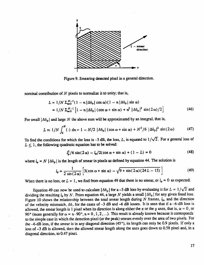
Figure 9. Smearing detected pixel in a general direction.
nominal contribution of N pixels to normalize it to unity; that is,
L 1/N _-t= Z,,=o(1 - n [A%[ cos a) (I - n [A_p[ sina)
= I/N Z_o' [I - n [A%[ (cos a + sin a) + n2 ]A%[ 2 sin(2a)/2] (46)
For small IA_p [ and large N the above sum will be approximated by an integral, that is,
L _ 1/N (.) dn = 1 - N/2 [A%[ (cos ot + sin a) + N2/6 [A%[ 2 sin(2a) (47)
To find the conditions for which the loss is -3 dB, the loss, L, is equated to 1/V_'. For a general loss of
L < 1, the following quadratic equation has to be solved:
I_/6 sin(2a) -_/2(cos a+ sin a) + (1 -/.,) = 0 (48)
where/!, = N [A% [ is the length of smear in pixels as defined by equation 44. The solution is
1 [ ]/_' = 2 sin(2a) 3(cos a+ sin o0 - _/9+ sin(2a)(24L - 15) (49)
When there is no loss, or L = 1, we find from equation 49 that there is no smear, or/_ = 0 as expected.
Equation 49 can now be used to calculate IAvi, I for a -3 dB loss by evaluating it for L = 1/V_" and
dividing the resulting/7, by N. From equation 44, a large N yields a small IA% I for any given fixed loss.
Figure 10 shows the relationship between the total smear length during N frames,/7,, and the direction
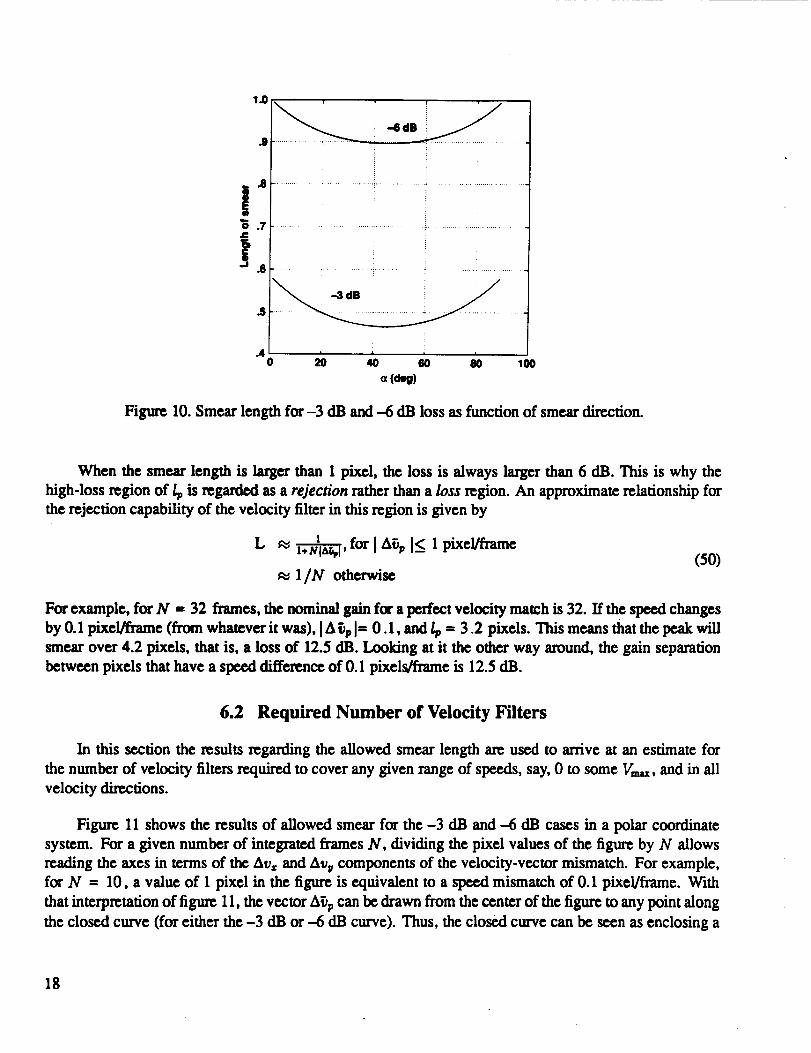
of the velocity mismatch, Ab, for the cases of -3 dB and --6 dB losses. It is seen that if a -6-dB loss is
allowed, the smear length is 1 pixel when its direction is along either the x or the _/axes, that is, a = 0, or
90* (more generally for a = n. 90", n = 0,1,2, ...). This result is already known because it corresponds
to the simple case in which the detection pixel (or the peak) smears evenly over the area of two pixels. For
the -6-riB loss, if the smear is in any diagonal direction (45"), its length can only be 0.9 pixels. If only a
loss of-3 dB is allowed, then the allowed smear length along the axes goes down to 0.58 pixel and, in a
diagonal direction, to 0.47 pixel.
17
1.0
.9
...8
.S
4ee !
................................. !......................................
i
.4 0 20 40 60 80J i
IO0
Figure 10. Smear length for-3 dB and -6 dB loss as function of smear direction.
When the smear length is larger than 1 pixel, the loss is always larger than 6 dB. This is why the
high-loss region of/_ is regarded as a rejection rather than a loss region. An approximate relationship for
the rejection capability of the velocity filter in this region is given by
L 1 for[ A_v [< 1 pixei/frameI+NIA_,I,
1/N otherwise(50)
For example, for N = 32 frames, the nominal gain for a perfect velocity match is 32. If the speed changes
by 0.1 pixel/frame (from whatever it was), [A _s, [= 0.1, and _ = 3.2 pixels. This means that the peak will
smear over 4.2 pixels, that is, a loss of 12.5 dB. Looking at it the other way around, the gain separation
between pixels that have a speed difference of 0.1 pixels/frame is 12.5 dB.
6.2 Required Number of Velocity Filters
In this section the results regarding the allowed smear length are used to arrive at an estimate for
the number of velocity filters required to cover any given range of speeds, say, 0 to some Vm_, and in all
velocity directions.
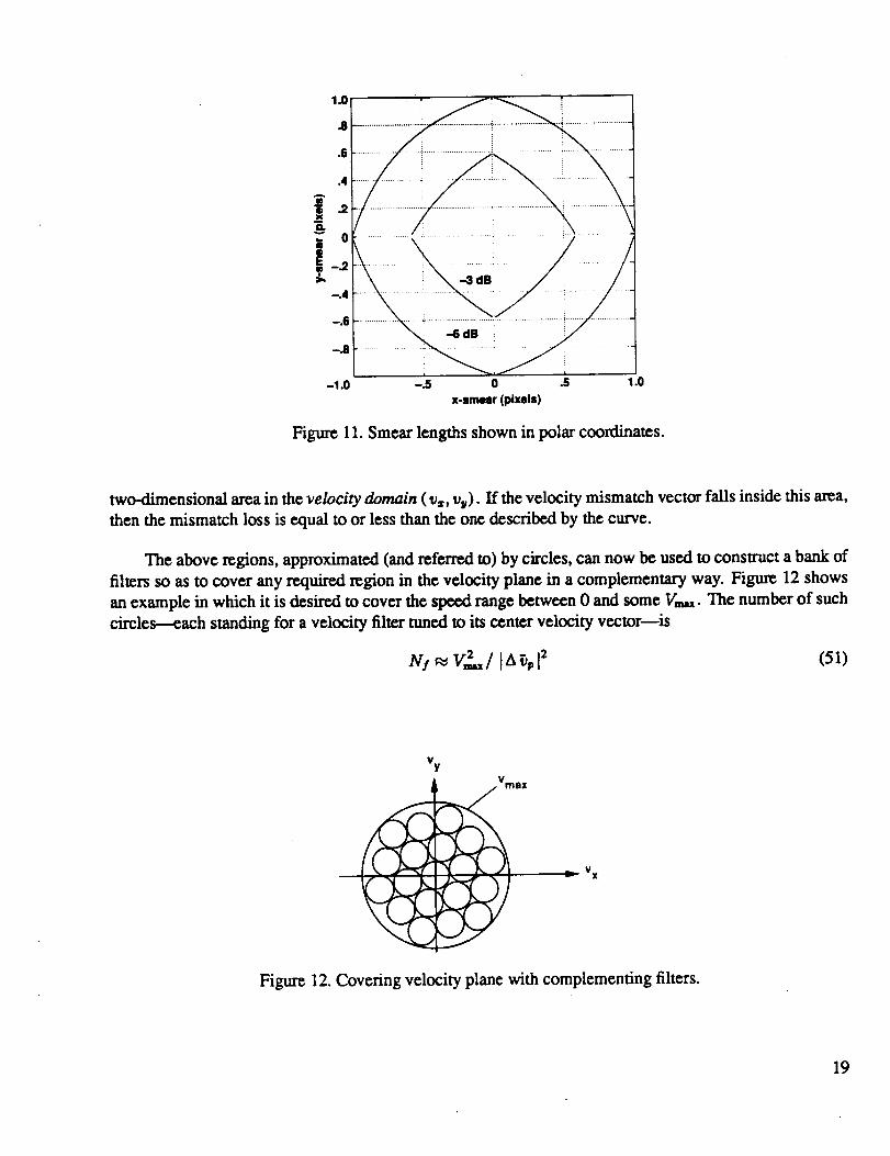
Figure 11 shows the results of allowed smear for the -3 dB and -6 dB cases in a polar coordinate
system. For a given number of integrated frames N, dividing the pixel values of the figure by N allows
reading the axes in terms of the Av= and Av U components of the velocity-vector mismatch. For example,
for N - 10, a value of 1 pixel in the figure is equivalent to a speed mismatch of 0.1 pixel/frame. With
that interpretation of figure 11, the vector A_p can be drawn from the center of the figure to any point along
the closed curve (for either the -3 dB or -6 dB curve). Thus, the closed curve can be seen as enclosing a
18
..........................; ! i
.e ........................i..................................i.....................
-1.0 -.5 0 .5 1.0
x-smear (pixels)
Figure 11. Smear lengths shown in polar coordinates.
two-dimensional area in the velocity domain (vz, v_). If the velocity mismatch vector falls inside this area,
then the mismatch loss is equal to or less than the one dcscdbed by the curve.
The above regions, approximated (and referred to) by circles, can now be used to consu'uct a bank of
filters so as to cover any required region in the velocity plane in a complementary way. Figure 12 shows
an example in which it is desired to cover the spe_d range between 0 and some V.m. The number of such
circles---each standing for a velocity filter tuned to its center velocity vector--is
2Ns _ v_/ IA_,.,I2 (51)
Vy
ax
v X
Figure 12. Covering velocity plane with complementing filters.
19
Forexample,if Y,.,., = 1 pixel/frame, and IA _I, I= 0.05 pix¢_e (for a 3 dB loss), then 400 filters
are needed to cover the reqttired range of velocity vectors. On the other hand, if it is required to cover
only a one-dimensional strip, as is the case for optical-flow calculations with a given focus of expansion,
then only Vm_/(2/p) filters are needed, where 2/_ is the diameter of the approximated "circle" filter of
figure 11. Continuing the above example, only 10 filters will be needed in that case.
6.3 Velocity Filter Algorithm
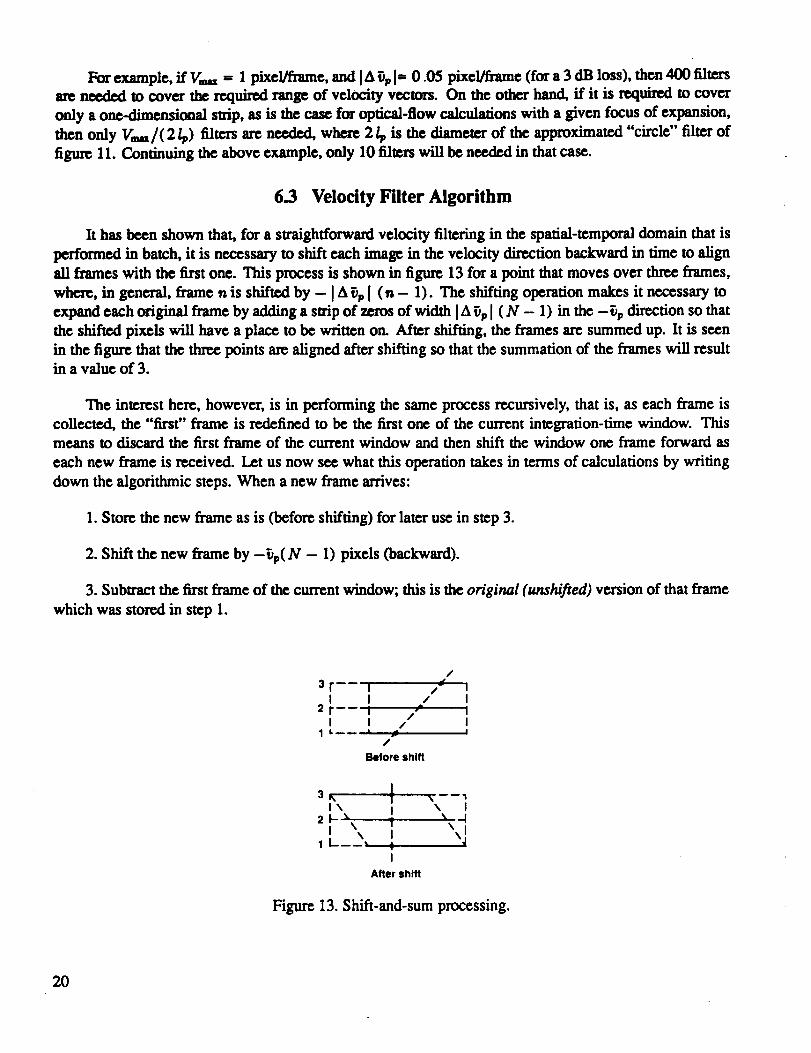
It has been shown that, for a straightforward velocity filtering in the spatial-temporal domain that is
performed in batch, it is necessary to shift each image in the velocity direction backward in time to align
all frames with the first one. This process is shown in figure 13 for a point that moves over three frames,
where, in general, flame his shifted by - IA pl (.- 1). Theshiftingoperation makes it necessary to
expand each original frame by adding a strip of zeros of width IA _j, I (N - 1) in the -_p direction so that
the shifted pixels will have a place to be written on. After shiftig, the frames are summed up. It is seen
in the figure that the three points are aligned after shifting so that the summation of the frames will result
in a value of 3.
The interest here, however, is in performing the same process recursively, that is, as each frame is
collected, the "first" frame is redefined to be the first one of the current integration-time window. This
means to discard the first frame of the current window and then shift the window one frame forward as
each new frame is received. Let us now see what this operation takes in terms of calculations by writing
down the algorithmic steps. When a new frame arrives:
1. Store the new frame as is (before shifting) for later use in step 3.
2. Shift the new frame by -_p(N - 1) pixels (backward).
3. Subtract the first frame of the current window; this is the original (unshified) version of that frame
which was stored in step 1.
/j,
3r-- i / II I / I
2r-- I /"J II I / I
/
Before shift
3e%I\
21-'_I \ \
11___
I \ I
\ II \_
IAfter shift
Figure 13. Shift-and-sum processing.
20
4. Shift thewindow frame by +_p (forward).
5. Sum up the window from step 4 to the result of step 2.
These steps can be written as
sum/÷1 = _÷l(sum_- _l) + sh_t._(.f'rc) (52)
where sumi and sum_÷l are the previous and updated sum frames, respectively, and sh denotes the shifting
operation in a direction indicated by the sign of its subscript (positive in the velocity-vector direction) and
by an amount given by the subscript size in units of _,. The frame fi'l above is the first frame of the old
window, and fro is the current new frame. The recursion can start from sum0 = 0, so that it builds up to a
steady state after the first N frames have been collected.
6.4 Computational Load and Memory Requirement
The computational requirements of the re,cursive algorithm described above will be determined in
this section. Starting with the computations rate, note that there are three basic types of operations: shift,
interpolation, and summation. The need for interpolation arises because the amount of shifting is generally
given by a non-integer number of pixels. Only one possible interpolation scheme is used here, and it should
be kept in mind that many others are also useful (discussed in section 8.4).
To shift a single pixel into some non-integer location requires the following algorithmic steps:
1. Get the pixel's location and value from memory.
2. Calculate the shifted-pixel non-integer (z, j/) location (two floating-point (FP) adds) and get the
remainders (Az, A_/) (two roundoffs).
3. Calculate intersection areas of the shifted pixel with the underlying 4 pixels, that is,
A = I+AzAy-Az-Ay
B = At/- AzAI/ (53)C = AzAy
D = _- AzA1/
which takes one FP multiplication and five FP adds.
4. Multiply the pixel's value by the four intersection areas (four FP multiplications).
5. Add these four values to the four underlying pixels (four FP adds).
Counting operations without distinguishing their types, a total of 18 operations are required to shift,
interpolate, and add 1 pixel. Since in equation 53 there is one add, one subtract, and two shifts, the total
number of operations that the re.cursive algorithm takes is 38 operations/pixel.
The rate of computations depends, of course, on the frame rate. If the frames come at R/frame/see,
and if M-pixel frames arc used, then the computations rate is 38 R/M operations/see per velocity filter,
21
or, for K filters,
Q = 38R/MK operations/see (54)
To get an idea about the order-of-magnitude of the required rate, we will use an example in which R! ---30frames/see, M = 512 × 512, and K = 400, which resolts in 1.19 • 10 n operations/see. Note, that a
computer with that capability is beyond the state of the art, and that these kinds of numbers create the
incentive to trade off performance for some possible reduction in the computation rate requirement.
The required memory can be written as
MEM = M(K + N) (55)
where the term MK represents K filters for which a single sum-frame of M pixels has to be stored,
and the term MN represents the storage of N original fi'ames so they can be subtracted as required by
equation 53). For the same example, and for N = 32 (N is the number of frames in the integrationwindow), MEM = 1.13 • 10 8 words.
7 APPLICATION TO THE OPTICAL FLOW PROBLEM
7.1 General
In this section, the general theory developed above is applied to the optical-flow problem. The optical-
flow case---under the assumption of a known focus-of-expansion (FOE)--offers various ways of reduc-
ing the computational requirement to a manageable level because it is basically a one- and not a two-
dimensional problem, at least in terms of the image coordinates. This means that only a one-dimensional
strip has to be covered in the velocity-vector plane that corresponds to a strip in the image plane. In other
words, the frames can be divided into some fixed number of angular sectors---all having the FOE as their
vertexmand then a bank of velocity filters applied so as to cover a linear strip in the velocity-vector plane
which is oriented the same as the sector in the image plane. This method of coverage is shown in figure 14
which is an overlay of the velocity and image planes. The -3-dB contours of the passband of the velocity
filters' are shown as circles, where the lowest-speed circle (besides zero speed) touches the origin so that
it corresponds to some minimum pixel distance from the FOE.
Each velocity filter in figure 14 is applied to all pixels underneath it. The product of the number offilters and the number of pixels, which determines the computational rate, stays constant if the filtering
process described by the figure is replaced by another one in which every pixel has its own dedicated filtercentered on it.
The optical-flow case is one-dimensional in the sense that the velocity direction is known for each
pixel; however, it has one additional dimension that has been ignored so far: the sensor/object range (or
depth, or distance). The simple filter-per-pixel processing could suffice if each pixel corresponded to a
unique velocity, but, because a pixel may represent objects at any depth, the pixel actually corresponds to
a range of velocities in the image plane. Thus, a set of filters is needed for each pixel to cover the range of
depths corresponding to that range of image-plane velocities.
The question now is how to cover the depth dimension for each pixel in the most efficient way. It willbe shown that, for any given depth, the pixel's speed in the image plane (or distance from the FOE) has
22
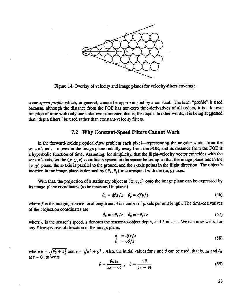
Figure 14. Overlay of velocity and image planes for velocity-filters coverage.
some speed profile which, in general, cannot be approximated by a constant. The term "profile" is used
because, although the distance from the FOE has non-zero time-derivatives of all orders, it is a known
function of time with only one unknown parameter, that is, the depth. In other words, it is being suggested
that "depth filters" be used rather than constant-velocity filters.
7.2 Why Constant.Speed Filters Cannot Work
In the forward-looking optical-flow problem each pixelmrepresenting the angular squint from the
sensor's axis---moves in the image plane radially away from the FOE, and its distance from the FOE is
a hyperbolic function of time. Assuming, for simplicity, that the flight-velocity vector coincides with the
sensor's axis, let the (_, y, z) coordinate system at the sensor be set up so that the image plane lies in the
( z, y) plane, the z-axis is parallel to the ground, and the z-axis points in the flight direction. The object's
location in the image plane is denoted by (Offi,0U) to correspond with the (z, y) axes.
With that, the projection of a stationary object at (z, y, z) onto the image plane can be expressed by
its image-plane coordinates (to be measured in pixels)
= 4fx/z = df lz (56)
where f is the imaging-device focal length and d is number of pixels per unit length. The time-derivatives
of the projection coordinates are
O, = vO,/z Ov = vOu/z (57)
where v is the sensor's speed, z denotes the sensor-to-object depth, and _ = -v. We can now write, for
any 0 irrespective of direction in the image plane,
0 = dfr/z
vO/z (58)
where 0 = _2 + 0v2 and r = 3/x 2 + y2. Also, the initial values for z and 0 can be used, that is, zo and 00
at t = 0, to write
0 Ooz0 0 v O= , = (59)zo - vt zo - vt
23
'mere is some minimum 0 for which these equations are meaningful, which corresponds to the velocity filter
whose circular -3-rib contour touches the origin 0 - 0 (the leftmost in figure 14. To find this minimum,recall from equation 44 that [A _p I-- l_/N pixelgframe. Since, for the minimum-speed pixel, O plays the
role of [A _p [, it follows that
/!, pixels/frame (60)00=
or, for a frame rate of R! frames/see,
0o = /_R----J'fpixels/sec (61)N
Replacing0 by 00 inequation59 and settingt = 0, givestheminimum processiblepixeldistancefromthe FOE as
0o=,= 17'z°R! pixels (62)vN
With typicalvaluesofz0 = 50 m,R! = 32 frames/see,v = 15 m/see,N = 16 frames,and/v _ 0.5 pixel
(asread from fig.10 fora -3-dB loss),00.,,- 3.33 pixels.This means thatforthegivendepth of
z0 = 50 m, allO'sbetween zeroand 6.66pixelsalongany radiuscenteredon theFOE willbe processed
by thesame lowest-speedvelocityfilter.
Next,we want tocheck how wellan acceleratingpixelhavinga hyperbolictimetrajectory,asgiven
by equation59,can be approximatedby a constant-s_ pixel.In otherwords,thelengthof timefor
which thepixel'sspeedremainsinsidea singleconstant-speedvelocityfilteristobe determined.
For a pixel found initially at 00, the initial speed is 00 = vOo/zo. If the speed were constant, 0 wouldincrease during N frames by 00N/R! pixels. On the other hand, the actual increase in 0 during N frames
is hyperbolic as given by equation 59, that is,
zoOo vN Oo- 00 = (63)
zo - vN/R/ zoR/- vN
Wc now want to limit the difference between the actual increase and its constant-speed approximation to
be less than/_, that is,
vOoN
vNOo vOoN
zo R! - vN zo R/
1 1 ] 00v2N 2
zoR/ - vN zo-RfJ- = zoR/(zoR! vN) < !_(64)
This leads to a quadratic equation for N with the result that
z°R/lr' [._[l + 4Oo/IT,-1]N< (65)
or, approximately,
(66)
24
The meaning of this bound is that with any larger N, the integrated energy over N frames will spill outside
of the constant-velocity-filter passband. Alternatively, for any given N there is an upper bound on 0. These
statements are clarified by the following example.
Example
For v = 10 m/sec, zo = 50 m, R! = 32 frames/see, 00 = 45 pixels, and/_ = 0.5 pixel, it is found
from equation (65) thatN _< 16, or that the integration time is less than 0.5 sec. Alternatively, forN = 16,
00 must be less then 45 pixels.
7.3 Using Velocity Profile Filters
Because we have seen that a constant-velocity filter can only be useful in limited cases (where either N
or 0o is small), it is suggested that variable-speed filters be used such that each filter is tuned to the velocity
profile generated by a hyperbolic time-function. First, it is realized that each hyperbola is determined (for
a given speed v) by the pixel's initial distance from the FOE, 00, and the range z0 of the object that this
pixel represents. Now the relevant problem is to find the passband of such a filter in terms of the range of
depths that will still fall inside it although it was tuned m some fixed depth z0. To answer this question,
the difference between two 0's calculated from equation 59 will be derived for a fixed 00 and v, but with
two different values for z0. One value is the tuned-for z0 itself and the other is some zb that denotes any
general value of z0 inside the filter's passband.
Thus, the passband of the velocity-profile filter is defined by requiring that the absolute value of the
difference between the above two 0's after T = N/R! seconds is less than/_ (lp defined as positive), or
Zb- I_<_Oh(T) - O(T) = Oo zb - _TZO .
z0 -vT] -</v (67)
When solved for the width of the passband in terms of sensor/object ranges, this inequality translates to
zu < zs _< z_ (68)
where the low end of the passband is
zo( 1 + 0o//_) - _Jv/RsZb/
+ 0o,-_/L -- 1uN
(69)
and the high end is
zo( 1 - Ooll.p) - vN/R s (70)z_ = _ - 0o//_ - 1
vY
Example
With v = 10 m/sec, N = 16 frames, R s = 32 frames/sec, 00 = 10 pixels, z0 = 50 m, and/1, = 0.5 pixel,
z_ = 36.0 m and z_h = 86.8 m. In other words, if a velocity-profile filter is tuned for a pixel at distance of
10 pixels from the FOE and for a nominal object range of 50 m, the passband (or bandwidth) of this filter
25
extends between 36 and 86.8 m. If a larger range of depths is to be covered for a pixel at the same radius,
several such filters have to be used and they have to be tuned to overlap, say, at their-3-dB points.
Figure 15(a) shows the time-evolution of the pixel used in the example above for the nominal, high,
and low object/sensor ranges. It is seen that after 16 frames, the pixel separation between the nominal
(center) graph and the graphs for the high and low depths are :!:/7, = 4-0.5 pixels. Figure 15(b) shows a
similar case except that 0o = 100 instead of 10 pixels and the depth bandwidth of the filter is only between
48.0 m and 52.1 m. It is thus seen that many more profile filters are needed to cover any given range of
depths for pixels that arc farther from the FOE.
Figure 16 shows the dependence of the number of profile filters needed to cover a given range of
depths on the pixel's distance from the FOE. The upper part of the figure shows horizontal lines with tic
marks. Consider, for example, the second such line from the bottom (corresponding to a pixel at a distance
of 20 pixels from the FOE) which is divided into four unequal segments by the tic marks. Starting from
the maximum depth of zt_ = 120 m in this example (the high -3-dB point of the highest-depth filter),
equation 70 is solved for the midpoint of the filter, z0. Notice that the solution of z0 in terms of z_ is the
same as that of zu in terms of z0 in equation 69. Now, using the zo = 77-m depth just found, zu is solved
for from equation 69 to find the low -3-dB point of the same (highest-depth) filter which is at z_ = 57 m.
This same point will also serve as the high -3 dB of the next filter below (in terms of depth) because all
filters are to overlap at their-3 dB points. Thus, equation 70 is used repeatedly to go down in depth in the
order of zbh, Zo, Zbl per filter, and the process continued for lower-depth filters until the required range
of sensor/object distances is covered. In this case, only two filters arc n_: i.e., the highest-depth filter
that covers the depths from 57 m to 120 m (with midpoint at 77 m), and the filter below that covers the
depths from 38.5 m to 57 m (with midpoint at 46 m). Thus, every three tic marks define one filter, and the
total number of filters requix_ is (approximately) half the number of tic marks.
The lower part of figure 16 shows the total number of filters that can be counted from the upper part.
It is seen that the total number of filters happens to be almost linear with the pixel's distance from the FOE,
and that the densities of the filters increase with the pixel's distance from the FOE and decreases with the
depth.
At this point it becomes apparent that the filter passbands, as seen in the upper part of figure 16, also
represent the accuracy with which the three-dimensional space in front of the sensor can be mapped. Each
filter can be thought of as a bin of the 3-D volume included in the FOV (two projection distances and
depth). As expected, the depth accuracy improves with increasing projection values (pixel's distance from
the FOE) and decreasing depth. There is always some minimum pixel distance from the FOE for which
only one filter (or actually half a filter) can cover the whole range of depths. There is no point in processing
pixels that are closer to the FOE because this minimum-distance pixel already corresponds to the coarsest
accuracy, or to an uncertainty the size of the whole range of depths of interest.
The next four figures (figs. 17 through 20) arc similar to figure 16 but with different parameters. The
following general behavior should be noted.
1. The number of filters increases with the speed, v.
2. The density of the filters increases as the depth decreases.
26
14.0
13.5
13.0
12.5¢:
o
_ 12.0
X
11.5
11.0
10.5
10.0
130 [
125
120
C
_o
115
K
110
105
IO00
................. •............................................ ! .....................
v : 10 m/s, 00 : 10 pixels, Rf : 32 fr/s
ZO, Ill
48.150.0
V = 52.1
b)
; 10 1; _0 is _0Frames (time)
35
Figure 15. Time-trajectories of a pixel receding from FOE for nominal and extreme object/sensor ranges:
v = l0 rn/scc, R/= 32 framcs/scc. (a) 8o = 10 pixcls, (b) 0o = 100 pixcls.
27
200
ul
,8=IP
II
100
E
5O
Range coverage for pixols by their distance from FOV
V : 10 rn/s
I_p = 0.5 plxolN :16fr
Rf : 32 fr/s
I1[11111111|111111111 I I I I I I I I I ! I I I ! I I I I I
I|lllPlllltlltllltllJlll I I t I I I I I I I I i ]
IIIIIlllllllllllllll I I I I I I | I I I I | I I
IIIIIIIIIIIIIIIitl 1 I I I I I I l I I I I I
IIIIIIIIlllllllll I I l I I I I I I i I
Illllllllllli I I I 1 I I J I 1 I I I
IIIIIIIItlll I I I I I 1 I I I I
[llllll I I i I I
I111 I I I I I I
Ill t I I I |
I I I I i I
I I 1 I I
I I
38.5 46L
1 !
I I
I I
I I
I
I I I I I
I I 1 I,
I I I
I I
I
I I57 77
0 20 40 60 80 100 120
Range coverage
2O
18
16
14m
=o 12k.
E
z 4
Number of profile filters by pixel distance from FOE
0 20 40 80 100 120 140 1 0 1 200
Initial-pixel distance from FOE
Figure 16. Number of filters rcquLrcd to cover a given range of sensor/object distances: v = 10 m/scc,
_, = 0.5 pixcl, N = 16 frames, R/= 32 framcs/scc.
28
160
140
120
uJ0u. 100E0
8_I=
mm•o 600X
E
35
3O
2O
z
5
Range coverage for pixela by their diltlnco from FOV
mmqlllllllllllllllllllllllllllllllll i i L I I I I I I J
msmqlllllllllllllllllllllllllllllll I I I 1 I I I I I
Ill|lllllllllllllllllllllllllll I I I I I I I I I I I 1 J
MIIIIlllllllllllllllllillllll I I I I I I I [
IIIIIlllllllllllllllllll I I I I I I I I I I I
IIIIIllllllllllllllll I I I I I t I I
Illlltlllllllll I I I I J I I
IIII11 I I I ] I I I I !
ill 1 ] ] I I
2'0 4'0 eo 80 lOO ,20 ,8oRange coverage
i i
Number of profile filters by pixel distance from FOE
v = 15 m/s
£p = 0.7 pixel
N =32fr
20 40 60 80 100 120 140
Initial-pixel distance from FOE
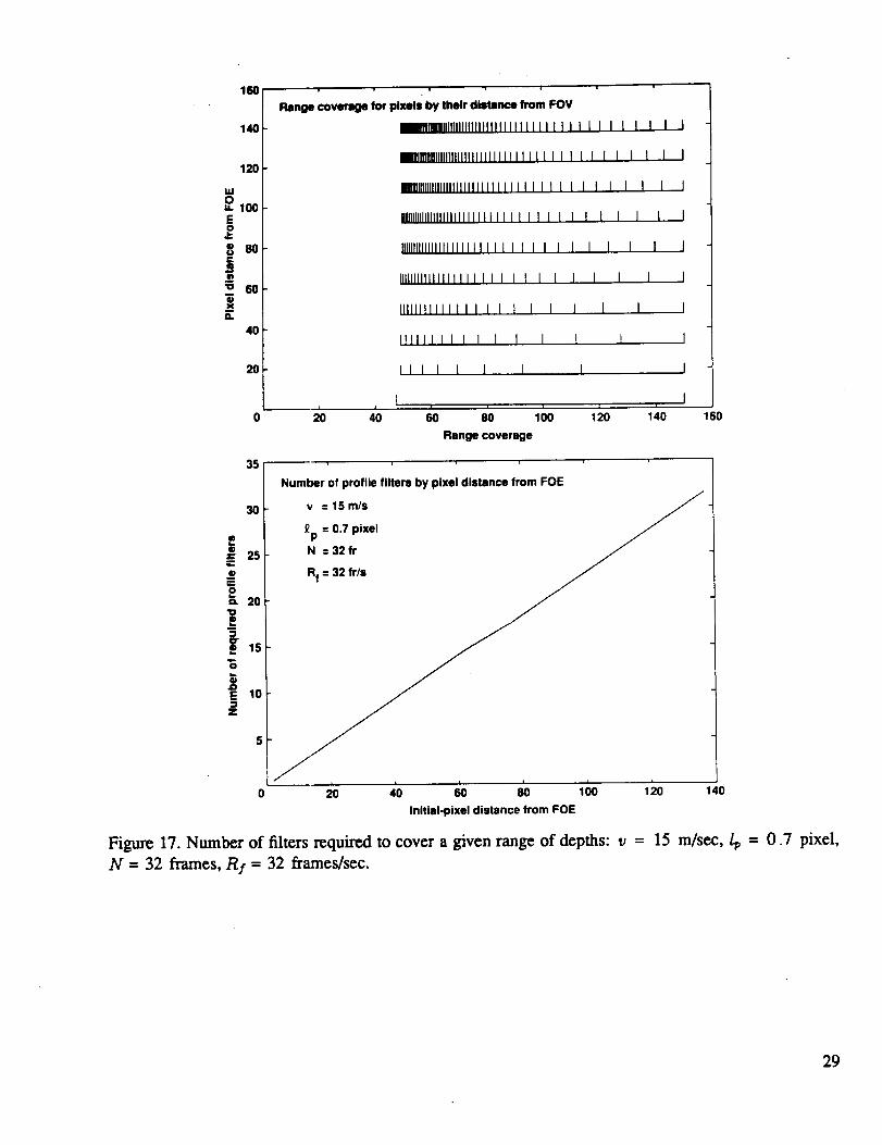
Figure 17. Number of filters rcquLreA to cover a given range of depths: v = 15 m/see,/1, = 0.7 pixel,
N = 32 frames, R/= 32 frames/sec.
29
IAI0U.
E
o0
16
"0
O.
160
140
120
100
8O
60
40
2O
Range coverage for pixeis by their distance from FOV
v :15m/s Hllillllllllllllillliliillllliil I I i I I I i
£p : 0.5 pixel
N :16fr
Rf : 32 fr/s
I I
[l[lllllllllllllltllllllllllI I I I I I I l I
lllllllllllllllllllllllI I I I I I l I I I
IIIIIIIIIIIIIIIIIII I I I I I I I I I
IIIIIIIIIIIIIII I I I I I I I I I
IIIIIIIII I I I I I I I I I I
IIIII I I I I I I I I I I
IIII I I I I I I
I I I I II
I
Range coverage
25
2O
5
Number of profile filters by plxel distance from FOE
; t i i i
20 40 60 80 100 120 140
Inltlel-plxel distance from FOE
Figure 18. Number of filters required to cover a given range of depths: v = 15 m/sex, _ = 0.5 pixel,
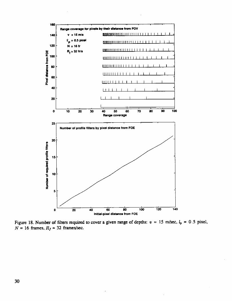
N = 16 frames, R/= 32 frames/sex.
3O
160
140
120
.io
_1ooo0u 80¢:a
-- 60o
O.
40
20
o
Range coverage for plxeis by their distance from FOV
v:15m/s IllJlllllll I I I I
l)p:l.0plxel Illllllllll I I lN =16fr
Rf = 32 fr/a I 11I I I I I I I
III1111 ] I
IIIII I t
III I I I
II I I 1
I I I 1
1 I
I I I I I [
I I I I 1
I I I I I I I
I I I I I I
I I I I 1
I I I I
1 I I
I I
I
lo 2'o _o _o _o _o _'o _o _o looRange coverage
12
10
Z
2
i
Number of profile filters by pixel distance from FOE
.... _ _o '20 40 60 1 120 140
Inltial-pixel distance from FOE
Figure 19. Number of fihcrs required to cover a given range of depths: v = 15 m/sea:,/,v = 1.0 pixel,
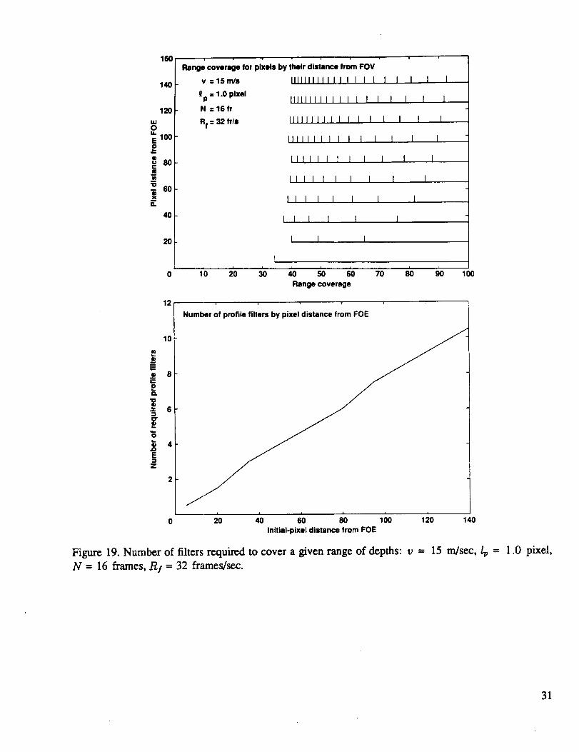
N = 16 frames, Rf = 32 frames/sec.
31
1110
140
120
UJO
'_ loo
l0
"O- 60ON
G.
40
20
30
25
E
Range coverage for pixela by their distllnce from FOV
v =15m/a _NIIIIIIIIIIIlilJJJllltlllll I I I I I I I I
£p : 1.0 pixel IgEItlllllllllllllllllllllllll I I I I I I I I I I I I IN =32fr
Rf = 32 fr/s
1() 2() 30
mlllllllllllllllllllllllllllllll I I 1 I I I I I I
nlllllllllllllllllllllllll I I I 1 I I 1 I
IIIIIII111111111111111111 1 I I I
Illlllllllllllllll I 1 1 I 1 I
ttilllitttll I I i I I t
lillll I f I I I I 1
III I I I I I
I I
I I
I I
I I I I
I I 1 I
I I I
I I
I | i r I ! |
40 50 60 70 80 90 100
Range coverage
Number of profile filters by ptxel distance from FOE
t i0 20 40 60 80 100 1_)0 140
Inillal-pixel distance from FOE
Figure 20. Number of filters required to cover a given range of depths: v = 15 m/sec,/_ = 1.0 pixel,
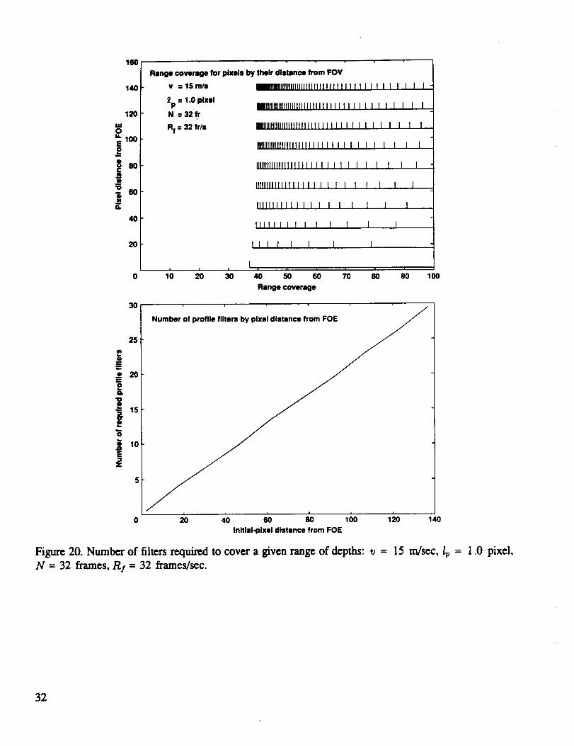
N = 32 frames, R! = 32 frames/sec.
32
3. The number of filters decreases as/1, increases because each filter is allowed to have a wider pass-
band; thus there is decreased gain at the ends of the passband.
4. The number of filters increases with the number of integrated frmnes N, because increasing N
makes a higher-gain and, thus, a narrower filler (for the same/_).
5. It is seen from equation 69 that increasing the flames' rate, R/, has the opposite effect of increasing
N.
8 ALGORITHM IMPLEMENTATION
8.1 Main Routines
The algorithm is implemented as follows. First, equation 69 is used repeatedly for all 1 _< 80 <__0,_=
to get the depth centers of all filters required to cover a given range of sensor-object depths. A 0,_= = 200
was chosen because pixels at that radius in the first flame will normally leave the FOV by the last frame,
and they are not processed anyhow. This can be described by the simple-minded "program" below.
input N, R I, I), 6
do for O0 = l,Onmz
Z = Zm=
until Z <_ Zmi .
Z = FUNCTION (Z)
enddo
The result of this part (SUBROUTINE ZFILTER) is stored in
1. nf(200) which gives the total number of depth filters needed for each 0 in the range of 1 to 200 pixels
distance from the FOE.
2. z(200,50) are the center depths for the same range of 0 and for up to 50 filters per 0.
The second part of the algorithm has the general form shown below.
DO FOR ALL PIXELS
convert cartesian coordinates of pixel with respect to the FOE
into polar coordinates; thus get distance and angle from the
horizontal axis in the image plane.
DO FOR ALL DEPTH FILTERS APPLICABLE TO THIS PIXEL
33
DO FOR ALL FRAMES
calculate pixel distance from FOE at this frame. Use
angle to convert from polar to cartesian coordinates.
read value of this pixel at this frame (interpolate).
same
store value to calculate statistics
END FRAMES' LOOP
calculate variance of pixels\rq\ values which were picked up
from the frames according to the depth filter in use.
record the minimum variance among all depth filters up to
current one and the corresponding depth for this pixel.
END OF DEPTH FILTERS LOOP
END OF PIXELS' LOOP
The criterion for choosing the depth for a pixel is that its gray level must be approximately con-
stant as it shows up in different locations in different frames. Thus, the depth-filer for which the ratio of
variance/average over the frames is the minimum is chosen.
8.2 Preprocessing
The original imagery cannot be processed directly by the velocity-filtering method. The reason is that
most practical imagery contains large objects (composed of many pixels), where each object is defined by
a nearly-consumt gray level. If we try to track any particular pixel found in the inside of the object, we
may associate it with other pixels belonging to the same object in the other frames instead of with its own
shifted versions, because the pixds are indistinguishable due to their similar gray level. This problem is
encountered not only for pixels that are completely inside the object but even for pixels found on the edges
of the object when their velocity vectors (away from the FOE) point toward the inside of the object. Sincethere is nothing to u'ack in a featureless region (inside of an object), this behavior of the algorithm is not
surprising. In fact, no algorithm can do better in such cases.
The natural thing to do in order to isolate features of an image is to employ some form of high-pass-
filtering (HPF). The signed-gradient operation, which is simply the spatial derivative along the radius from
the FOE, was chosen. This direction is chosen because each velocity filter picks up pixels from different
frames along such lines. Thus, a "featu_" is a variation in gray level in the radius direction. Two different
methods of gradient-based preprocessing are considered here; they are discussed in the following.
34
Gradient operation. Straightforward gradient processing as described above brings up the features
needed for velocity filtering but it has a crucial drawback when the preprocessed images are later processed
with the main velocity-filtering algorithm. The problem is that close objects are always observed on the
background of farther objects found behind them. The background objects, since they are farther from
the sensor, move at lower speeds away from the FOE than the close objects. As a result, the gray-level
differences at the edges of the close objects change with time as different background objects pass by
behind the close object. In other words, the edges of objects, as obtained from the gradient operation,
have a varying gray level over different frames, thus, they cannot he used with any algorithm that relies
on constant gray level for every object over all frames. Only in unrealistic cases, in which the scenery is
composed of nonoverlapping objects situated against a uniform background, will the simple gradient work.
For this reason, the alternative discussed below is considered.
Gradient used only as a test. Another way of obtaining the feature-rich parts of the imagery is to
use the gradient as a test in choosing the edges out of the original nongradient imagery. This is done by
zeroing out all parts of the original imagery that do not have a gradient (its absolute value) above some
threshold. It is important to emphasize that the featureless parts of the images have to he actually zeroed
out; processing them cannot be simply skipped, for the reason explained earlier regarding edge pixels that
move into the inside of the object.
8.30bject's Expansion Between Frames
The linear dimensions of an object grow inversely proportional to the depth. Some comments are in
order in this regard.
First, there is the question of compliance with the sampling theorem. Since the objects in all practical
cases can be of any size, there will always be some objects that are smaller than a pixel; thus, there is the
potential of aliasing. A simple way to avoid aliasing is to blur the optical point-spread function (PSF) in
front of the sensor so that it is larger than two pixels.
Assume, for example, an object with a perfect (step-function) edge. Using a PSF of the above size
will make this edge show up in roughly two pixels---irrespective of the size of the object itself, which
increases with time. Thus, in such an ideal case, the algorithm does not have to accommodate for the
object' s growth between frames. However, if an object is assumed that has a gradual gray-level transition
at its edges which span a few pixels, the size (or width) of the edges will grow with time. In such a case
the algorithm does have to accommodate for the object' s growth between frames. Moreover, in this case
the different amplitudes of the gradient images at different depths must be compensated for. The reason is
that an edge changes its width in terms of pixels as the depth changes, but it always describes an overall
fixed gray-level difference between the two objects of the nongradient image which are found at both sides
of the edge.
The problem is that there will always be a mix of object edges that fall into the above two categories.
Moreover, every non-ideal object goes from the category of sharp-edges to that of the wide-edges as it
approaches the sensor. Thought has been given to an edge-width test for determining the category, but it
has not been tried out as yet. For the purposes of this report each category was simply used separately for
the whole run.
35
8.4 Methods of Interpolation
The need for interpolation arises because spatial _mples (pixels) of the physical scene are being dealt
with. Since any discernible change of gray level in the image is defined to be an isolated object, it must be
possible to deal with small objects of the order of 1- to 3-pixels. When considering edges, this size refers to
the width of the edge. Thus, there is no point in trying to estimate the gray levels of the underlying objects;
instead, the pixel readings themselves must be used to describe the gray levels of the physical object.
First method. If a pixel at frame No. 1 is considered to be the object itself or a part of the object,
then this "object" (pixel) will normally intersect 4 pixeis of any later frame as it moves with the optical
flow. For the add-and-shift algorithm, the gray level of the object must be read at all flames. The question
is what to do when the original pixel-object is expected to fall in between 4 pixels---that is, there are
four observations that are affected by the original pixel's gray level, but they are also affected by other
unaccounted-for pixels. The gray-levels of these other pixeis that contribute into the four observed pixels
can be thought of as random variables having a zero mean. The point is that by interpolating the values of
the four observed pixels, a random variable is obtained having an average equal to the tracked pixel gray
level and some variance.
Tracking a pixel-object through the frames means summing up its interpolated gray levels over all
frames, that is, summing up N random variables. The variance of the sum variate (normalized by the
average) _es proportionate to N. Since the test for assigning depth to a pixel makes use of the
sample variance (which is itself a random variable), there is some probability of wrong depth assignment
associated with the randomness of the interpolation scheme described above.
As explained above, the origin of depth-assignment errors is in the interpolation scheme which is
based on 4 pixels. Note that the u'acked object-pixel occupies only one fourth of the area of these 4 pixels,
whereas three fourths of the area is random. One obvious way to increase the ratio between nonrandom
and random pixel areas involved in the interpolation is to define the object to be larger than one pixel,
say 2 × 2 pixels. In such a case the above ratio increases from 1/3 to 4/5 because 9 pixels must now be
observed instead of 4.
The definition of an object as a square of 2 × 2 pixels has a side effect in the form of blurring the
image or low-pass filtering (LPF) it. This is why it is not suggested to go on and define 3 × 3 pixels, for
example, as objects. It was found that a 2 × 2 size is a good compromise because with smaller objects the
sampling theorem limits are encountered, and with larger ones the image is too blurred.
So far the effect of object expansion (or growth) on the interpolation process has been ignored. If this
factor, is to be included, more than 4 pixels must be used. What is done in the algorithm is to observe all
pixels in the current frame that have any common area with the expanded pixel tracked from frame 1, and
to then interpolate on these pixcls.
Second method. Another method was tried that avoids, at least in principle, the randomness associ-
ated with the first method above. Here it is, assumed that the minimum-size object at frame 1 is 2 × 2 pix-
els. At any later frame this object occludes at least 1 pixel of the later frame completely. This means that,
given the gray-level values of the 4 pixels from frame-l, their contribution to the later-frame pixelcan be
calculated proportionately to their intersected area with that pixel.
36
The performance of this method was poor compared with that of the first method. Its sensitivity to the
assumption that the underlying object can be described by the values of 4 pixels appears to be the reason.
Here, the actual gray levels of the 4 pixels from frame 1 are used to predict the gray level of a pixel in a
later frame, whereas in the first method we essentially work with the sums of the 4 pixel gray levels.
8.5 The Algorithm Parameters
This section lists all the algorithm parameters that have to be chosen and explains the considera-
tions associated with their choice. When working with either the gradient images themselves or with the
gradient-as-a-testmethod, itis necessary to specifythe FOE and the threshold,Gth, under which the
gradient value will be set to zero.
For the main algorithm it is necessary to choose the following parameters (in addition to specifying
the FOE):
I.Beginning and end rows and columns of theimages thatare to be processed.
2. Gth: Threshold on theabsolutevalue of thegradientimagery under which pixelvaluesarc setto
ZerO.
3. Rth: The threshold on the ratio of tins/average (of object gray levels over all frames) under which
the corresponding depth-filter is not allowed to be considered for a pixel. If this parameter is chosen too
low (say, 0.1), more first-frame pixels are never assigned a depth; thus, they will appear blank in the final
depth image. However, those pixels for which this ratio (for any depth filter) goes under the threshold will
have good depth estimates. If this parameter is chosen high (say, 0.6), it allows almost all pixels to get a
depth estimate but these estimates are, in general, less reliable.
4. Side:The sidesizeinpixelsof the minimum-size object(2means 2 x 2 pixelobjects).Choosing
thisparameter to be I causes the depth estimatefora largepercentage (10% to 20%) of the pixelsto be
in error, meaning completely wrong depths. Choosing it to be 2 yields much better results because it does
spatialLPF (orpixelaveraging)along withdecreasingtheerrorvarianceassociatedwith the interpolation.
Choosing thisparameter tobe 3 orhighereffectivelyblurstheimage excessivelyand averages out objects
with their(time-varying)background atthe edges; thus,itundermines the essentialpremise of constant
gray levelover allframes.
5. z,,,..,and z,,,_,,,thatis,maximum and minimum depths:These parameters determine the range of
depths over which centersof depth filterswillbc precalculatecLSince a fixednumber of depth filtersis
aUowcd and sincecalculatingof theircentersstartfrom z,,_._going down, itusuallyhappens thatforlarge
0's,alldepth filtersare consumed beforearrivingatz,,,/n.This iswhy itisnecessaryto"focus" the choice
of depthsrange so thata limitedrange of interestiscovered.
6./v: This is the width of the depth filter which is used here to define the separation between two
adjacent depth filters, as explained in section 6. Choosing this parameter to be 0.5 or I pixel for example,
causes the depth filters to overlap at their-3 dB or-6 dB points, respectively (see fig. 10). Obviously,
when a higher _ is chosen, coverage of the depths' range is allowed with fewer filters. This makes the
algorithm more efficient but less accurate in terms of pixcls' depth assignment.
37
7. R t, or fxames' rate in frames per second: This parameter is the acuml famncs' rate, so there is nochoice to be made.
8. _, or the vehicle's speed in meters per second: Again, this is the actual vehicle's speed.
9. N or number of fi'ames: The algorithm is working in batch for a fixed number of frames, so that N
is given by the choice of the data set itself.
I0. Expand: Equals 1 when taking into account object expansion with decreasing depth; equals 0
otherwise.
8.6 Data Sets Used
Two dam sets were used. One is the 15-frame imagery taken at the NASA/FSN image processing
laboratory (pencils on a table) and the second is the SRI data set (ladder and thrown shin) that originally
contained 128 images. To limit the number of processed frames in the SRI set, only every other frame of
the last 64 frames was used, thus reducing this set to 32 frames. This section summarizes the results of a
few hundred runs by presenting the final product of some representative cases in the form of a depth imagebased on frame No. 1 of each set.
Data set scaling. In order to use a data set that was taken in a laboratory environment, it was necessary
to scale it in terms of vehicle speed, frame rate, and distances. The general formula for the depth scalefactor is
S = _ (71)Rlvt
where v is the vehicle's actual speed in meters per second, vl is the lahomtory speed of the ¢mmem in meters
per frame,and R/is the laboratoryframes rateinframes per second,which isassumed equal tothe actual
fxame rate.
In the case of the FSN data set, the images were taken every 1.25 cm. If R/= 1 frame/sec is chosen
arbitrarily, the lab speed is vi = 0.0125 m/frame. Similarly, if v ffi 10 m/sec is arbitrarily chosen, then
S ffi 800. The above arbitrary choices cause z,u and z,i, to be chosen accordingly, and affect the depth
scaling of the output but not the essential results. Given that the depths of relevant objects in this set are
between 0.33 and 0.9 rn (at the first flame), this translates to 260 and 720 m, respectively.
The original512 x 512 imagery was reduced to 256 x 256 by averagingevery 4 pixelsintoa single
pixel.The FOE for thereduced imagery isatrow = 105 and col = 120.
In the case of the SRI imagery, vt = 10.16 •10 -3 m/frame, and R/= 32 frames/sec(usingevery
otherframe).Ifv = I0 m/see,thescalefactorisS = 30.76. The FOE forthereduced 256 x 256 imagery
of thissetisatrow = 107 and col = 115.
Results for the FSN imagery. The original images (first and last) are shown in figures 21 and 22,
and their gradient versions thresholded above 4 (the gray-level rms is 35) are shown in figures 23 and 24.
Figures 25 and 26 show the original first and last frames in the parts that have an absolute gradient valuesabove 5.
38
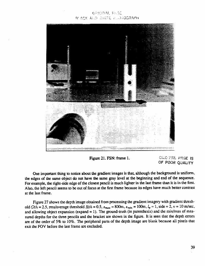
R ' LC!< Ai.:_:) L:i.I;-_E. ,: .... )(OGRAPH
Figure 21. FSN: frame 1.
OF POOR QUALITY
One important thing to notice about the gradient images is that, although the background is uniform,
the edges of the same object do not have the same gray level at the beginning and end of the sequence.
For example, the right-side edge of the closest pencil is much lighter in the last frame than it is in the first.
Also, the left pencil seems to be out of focus at the first frame because its edges have much better contxast
at the last frame.
Figure 27 shows the depth image obtained from processing the gradient imagery with gradient thresh-
old Gth = 2.5, rms/average threshold Rth = 0.5, z,,_= = 800m, z=_,, = 100m,/_, = 1, side = 2, v = 10 m/sec,
and allowing object expansion (expand = 1). The ground-truth (in parenthesis) and the min/max of mea-
sured depths for the three pencils and the bracket are shown in the figure. It is seen that the depth errors
are of the order of 5% to 10%. The peripheral parts of the depth image are blank because all pixels that
exit the FOV before the last frame are excluded.
39
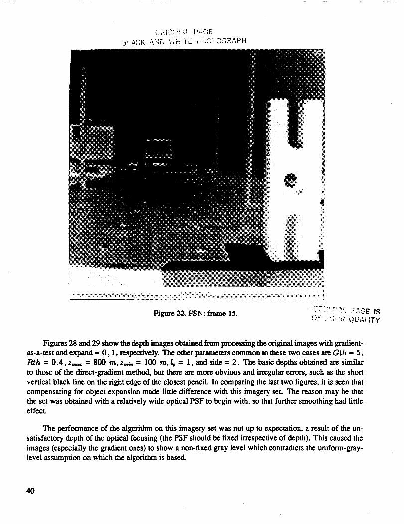
BLACK AND '_,'I-ti-IE r-f-,O,u_RAPH
Figures 28 and 29 show the depth images obtained from processing the original images with gradient-
as-a-test and expand = 0,1, respectively. The other parameters common to these two cases are Gth - 5,
Rth = O .4, z,_z = 800 m, z,,,_,, = 100 m, g = 1, and side = 2. The basic depths obtained are similar
to those of the direct-gradient method, but there are more obvious and irregular errors, such as the short
vertical black line on the right edge of the closest pencil. In comparing the last two figures, it is seen that
compensating for object expansion made little difference with this imagery set. The reason may be that
the set was obtained with a relatively wide optical PSF to begin with, so that further smoothing had little
effect.
The performance of the algorithm on this imagery set was not up to expectation, a result of the un-
satisfactory depth of the optical focusing (the PSF should be fixed irrespective of depth). This caused the
images (especially the gradient ones) to show a non-fixed gray level which contradicts the uniform-gray-
level assumption on which the algorithm is based.
40
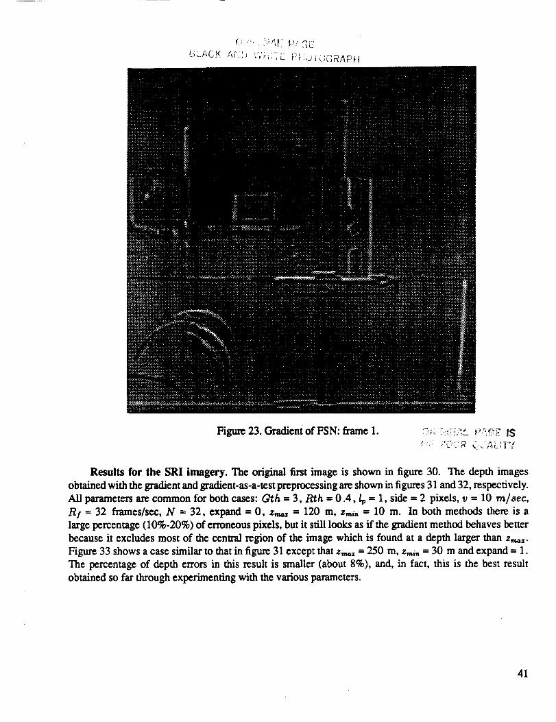
• ._ t.2
Figure 23. Gradient of FSN: frame 1.
Results for the SRI imagery. The original first image is shown in figure 30. The depth images
obtained with the gradient and gradient-as-a-test preprocessing are shown in figures 31 and 32, respectively.
All parameters are common for both cases: G-_h = 3,/_h = 0.4,/1, = 1, side = 2 pixels, v = 10 rn/sec,
Rf = 32 frames/see, N = 32, expand = 0, z,,_ = 120 m, zmi,, = 10 m. In both methods there is a
large percentage (10%-20%) of erroneous pixels, but it still looks as if the gradient method behaves better
because it excludes most of the central region of the image which is found at a depth larger than z,_z.
Figure 33 shows a case similar to that in figure 31 except that z,,_ = 250 m, zmi,_ = 30 m and expand = 1.
The percentage of depth errors in this result is smaller (about 8%), and, in fact, this is the best result
obtained so far through experimenting with the various parameters.
41
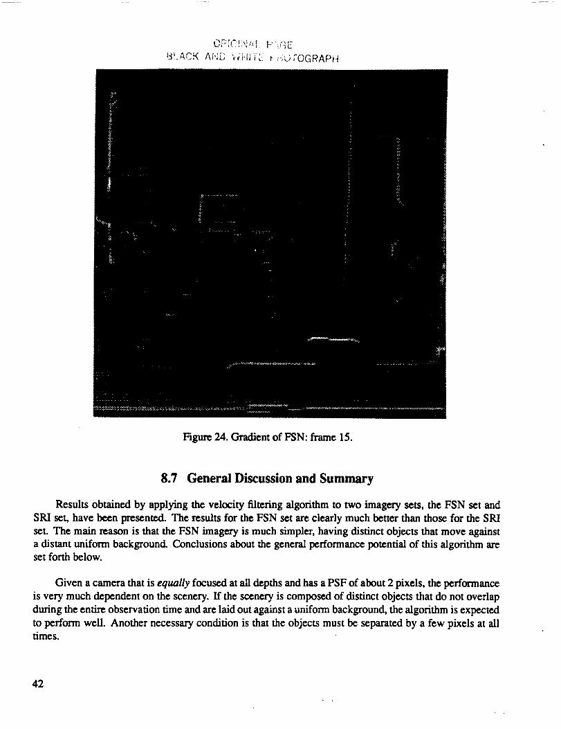
OF-_7,'.!! ['j.,'._'[_ P...qE
B1.A,.";,K A#'_D _,#i-I;i-E r: :-;O ,"OGRAPH
Figure24. Gradient of FSN: frame 15.
8.7 General Discussion and Summary
Results obtained by applying the velocity filtering algorithm to two imagery sets, the FSN set and
SRI set, have been presented. The results for the FSN set are clearly much better than those for the SRI
set. The main reason is that the FSN imagery is much simpler, having distinct objects that move against
a distant uniform background. Conclusions about the general performance potential of this algorithm are
set forth below.
Given a camera that is equally focused at all depths and has a PSF of about 2 pixels, the performance
is very much dependent on the scenery. If the scenery is composed of distinct objects that do not overlap
during the entire observation time and are laid out against a uniform background, the algorithm is expected
to perform weLl. Another necessary condition is that the objects must be separated by a few pixels at alltimes.
42
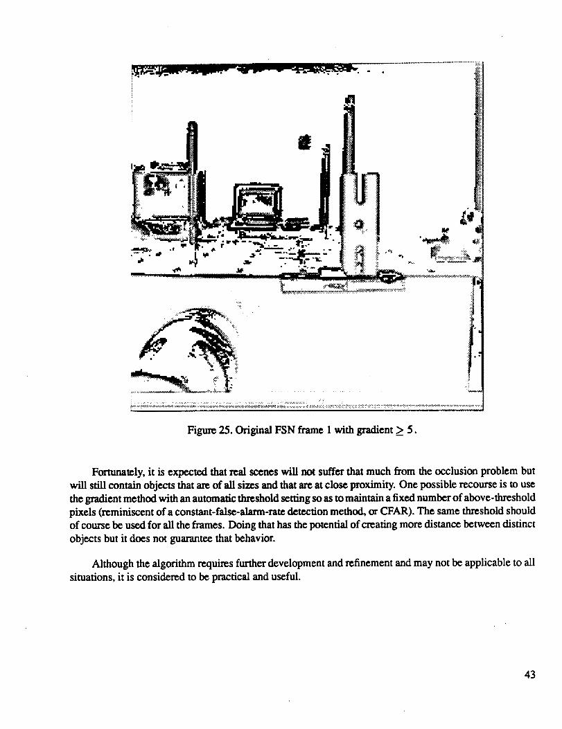
Figure 25. Original FSN frame I with gradient __ S.
Fortunately, it is expected that real scenes will not suffer that much from the occlusion problem but
will still contain objects that are of all sizes and that are at close proximity. One possible recourse is to use
the gradient method with an automatic threshold setting so as to maintain a fixed number of above-threshold
pixels (reminiscent of a constant-false-alarm-rate detection method, or CFAR). The same threshold should
of course be used for all the frames. Doing that has the potential of creating more distance between distinct
objects but it does not guarantee that behavior.
Although the algorithm requires further development and refinement and may not be applicable to all
situations, it is considered to be practical and useful.
43
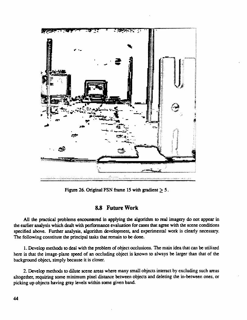
• ii
]
..... ii
Figure 26. Original FSN frame 15 with gradient > 5.
8.8 Future Work
All the practical problems encountered in applying the algorithm to real imagery do not appear in
the earlier analysis which dealt with perfcxmance evaluation for cases that agree with the scene conditions
specified above. Further analysis, algorithm development, and experimental work is clearly necessary.
The following constitute the principal tasks that remain to be done.
1. Develop methods to deal with the problem of object occlusions. The main idea that can be utilized
here is that the image-plane speed of an occluding object is known to always be larger than that of the
background object, simply because it is closer.
2. Develop methods to dilute scene areas where many small objects interact by excluding such areas
altogether, requiring some minimum pixel distance between objects and deleting the in-between ones, or
picking up objects having gray levels within some given band.
44
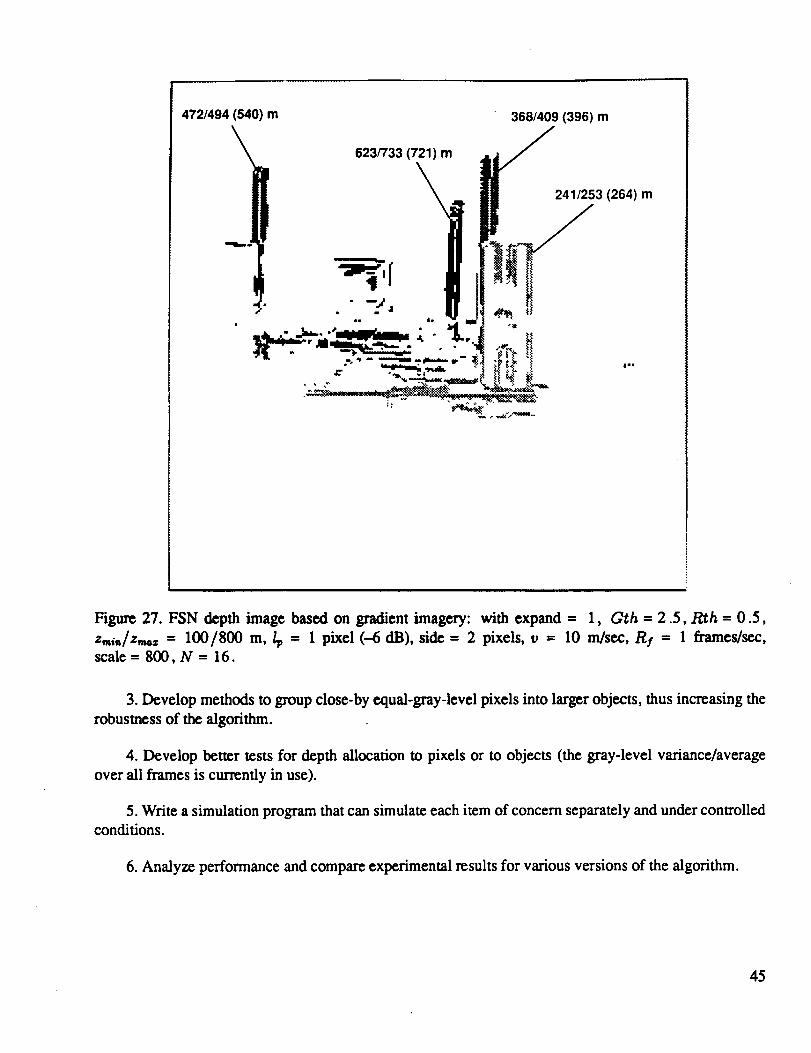
472/494 (540) m 368/409 (396) m
Figure 27. FSN depth image based on gradient imagery: with expand = 1, Gth = 2.5, tith = 0.5,
z=i,,/z,,_= = 100/800 m,/1, = 1 pixel (--6 dB), side = 2 pixels, v = 10 m/sec, R! = 1 frames/see,scale = 800, N = 16.
3.Developmethods togroupclose-byequal-gray-levelpixclsintolargerobjects,thusincreasingthe
robustnessof thealgorithm.
4. Develop better tests for depth allocation to pixels or to objects (the gray-level variance/average
over all frames is currently in use).
5. Write a simulation program that can simulate each item of concern separately and under controlledconditions.
6. Analyze performance and compare experimental results for various versions of the algorithm.
45
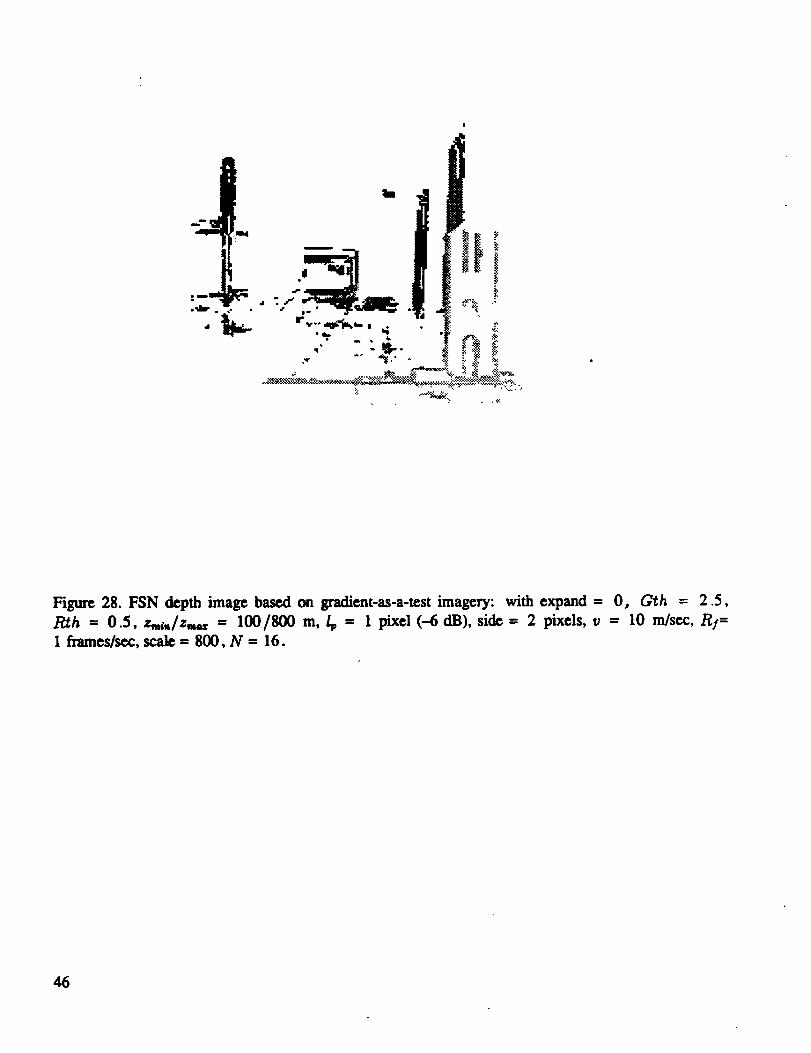
Figure28. FSN depth image based on gradient-as-a-testimagery: with expand = 0, Gth = 2.5,
Rth = 0.5, zmi,,/z,,_= I00/800 m,/_,= I pixel(--6dB), side= 2 pixels,v - I0 m/sec,R/=
1 frames/sec, scale = 800, N = 16.
46
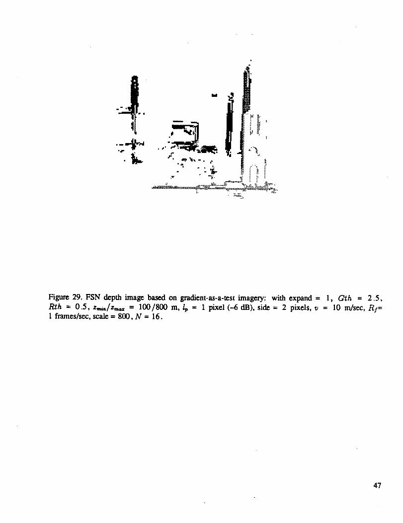
Figure 29. FSN depth image based on gradient-as-a-test imagery: with expand =
Rth = 0.5, z=i,,/z,,_ = 100/800 m,/I, = 1 pixel (-6 dB), side = 2 pixels, v1 frames/see, scale = 800, N = 16.
1, Gth = 2.5,
= 10 m/see, Rf=
47
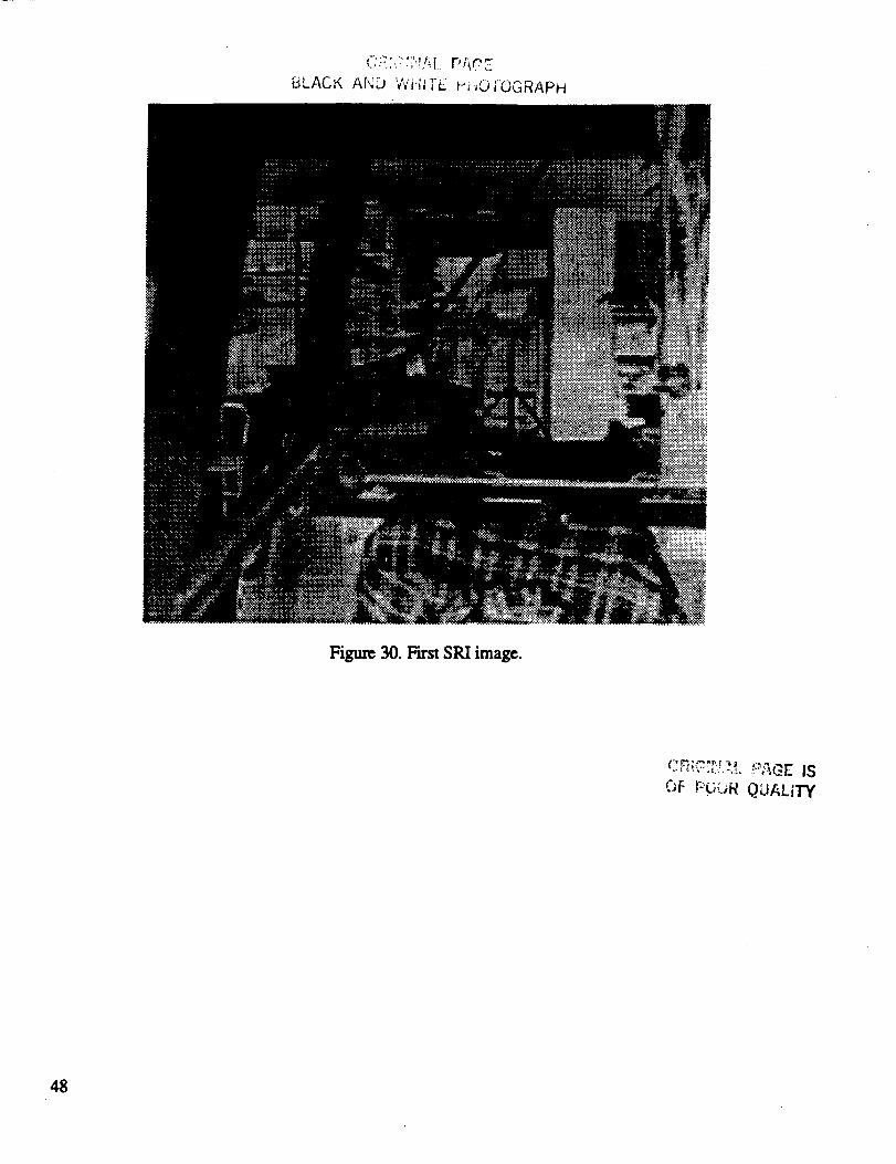
BLACK Alqb WHITE _"_-iO;-OGRAPH
Figure 30. First SRI image.
OF P¢;bR QUALITY
48
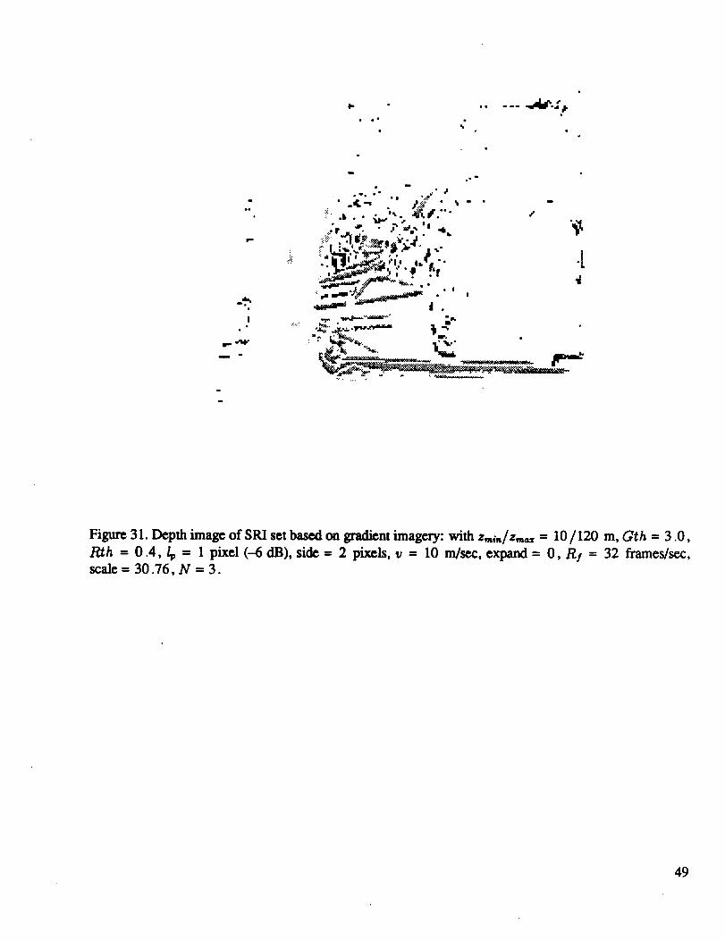
• i • .
%
i
o.
_.--.
I
i_ .sq,,
I
• ° i
• • Ii" ?_ _ I
•,__, ,,,_ _,,".__',_: .'"
• .
.__._-,_ _-_=: _ _._. _. .
" _ _"~'_ "_"" L._ _ ._
Figure 31. Depth image of SRI set based on gradient imagery: with z,_/z_= = 10/120 m, Gth = 3.0,
Rth = 0.4, _ = 1 pixel (-6 dB), side -- 2 pixels, u = 10 m/sec, expand = 0, R/ = 32 frames/sec,
scale = 30.76, N = 3.
49
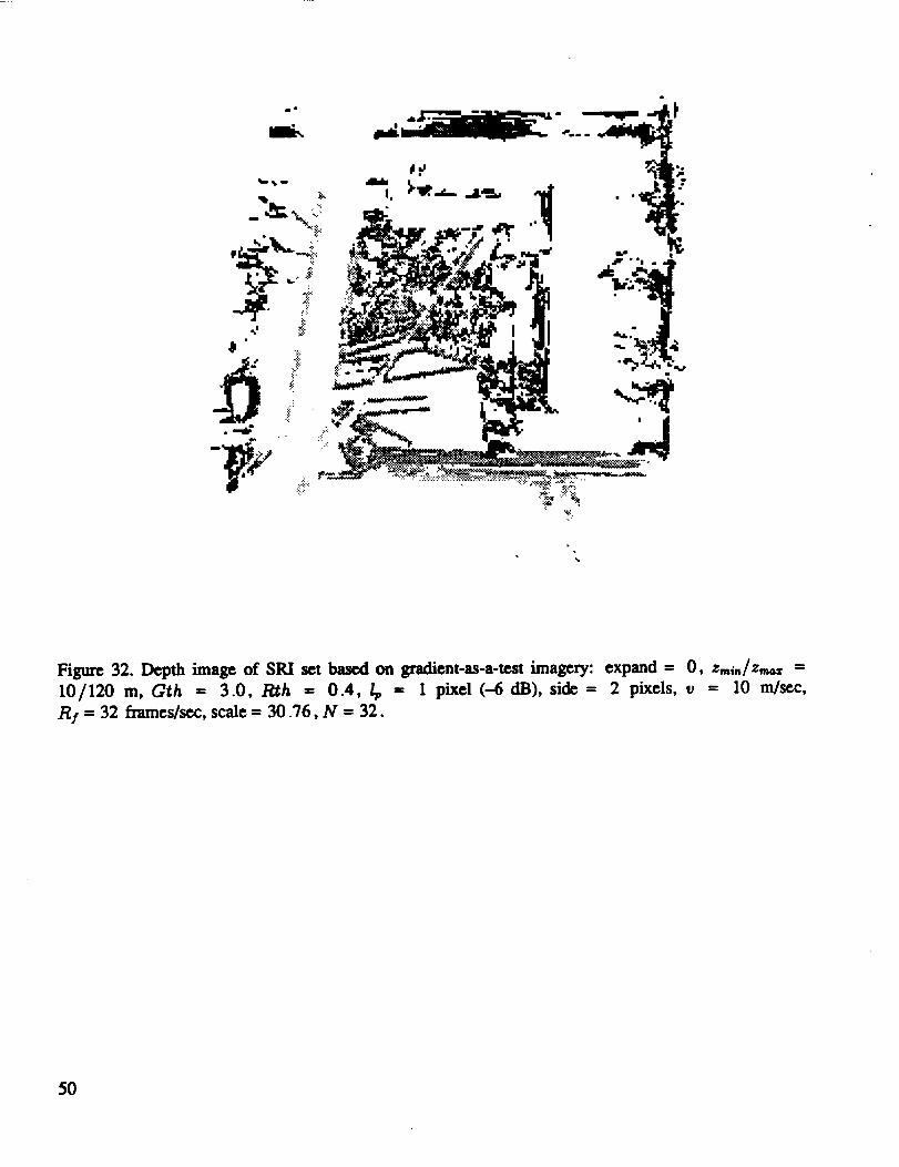
Figure 32. Depth image of SRI set based on gradient-as-a-te_imagery:
10/120 m, Gth = 3.0, I_h = 0.4, /_,= 1 pixel(--6dB),side=
R/= 32 frarnes/sec,scale= 30.76, N --32.
expand = O, z,._./z,== =2 pixels, v = I0 m/sec,
5O
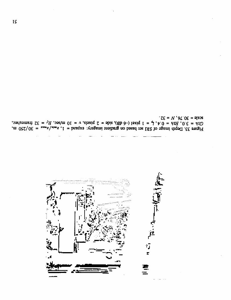
"Z£ = N '9L'0£ = oI_S
'_os/sou._xj Z£ = t_ '_sp.u 0I = a 'SlOx!.d Z = _!s '(_ 9-)IOx!.d I = _/'_'0 = V_ r '0"_ = V_
'w O_Z/O_ = _z/_:=z 'I = pu_dxa :_o_u_. maq_z_ uo lY_q _s I'dSjo o_u_. q_do(l"_ _un_!.4
,l__lii _. __m = ---- -...='B'_" "_l_
REFERENCES
1. Reed, L S.; R. M. Gaglianti; and H. M. Shao: Application of Three-Dimensional Filtering to Moving
Target Detection. IEEE Trans. Aerosp. and Electronic Sys., vol. AES-19, no. 6, Nov. 1983,
pp. 898-905.
2. Watson, A. B.; and A. J. Ahumada, Jr.: Model of Human Visual-Motion Sensing. J. Opt. Soc. Am,
A, vol. 2, no. 2, Feb. 1985, pp. 322-341.
3. Porat, B.; and B. Friedlander:. A Frequency Domain Approach to Mulfifimne Detection and Estima-
tion of Dim Targets. ICASSP, Apr. 1987
4. Reed, L S.; IL M. Gagliardi; and L. B. Stotts: Optical Moving Target Detection with 3-D Matched
Filtering. IEEE Trans. Aerosp. and Electronic Sys., vol. AES-24, no. 4, July 1988, pp. 327-335.
5. Stotts, L. B.; I. S. Reed; and R. M. Gagliardi: Air Vehicle Detection by Using an Ensemble of Moving-
Picture Images. NOSC TR-1163, Jan. 1987.
6. Kendall, W. B.; and W. J. Jacobi: Passive Electro-Optical Sensor Processing for Helicopter Obstacle
Avoidance. Space Computer Corporation, Santa Monica, Calif., Dec. 1988.
7. Bracewell, R.: The Fourier Transform andlts Applications, McGraw Hill, 1965, pp. 69-90.
8. Papoulis, A.: Systems and Transforms in Optics. McGraw Hill, 1969.
9. Wozenerafi, J. M.; and I. M. Jacobs: Principles of Communication Engineering. Wiley, 1965,
pp. 229-231.
10. Nahi, N.E.: Estimation Theory and Applications. W'dey, 1969.
52
Report Documentation PageImemmmemlWl
1. Report No.
NASA TM-102802
4. Title and Subtitle
2. Govmmmer_ Aooo_Jon No.
Velocity V--dte_g Applied to Optical Row Calculations
a. _r= ca_ No.
s. Ream Dm
7.Author(t)
Yah" Barniv
9. Performing Oeganizalion Name and Address
Ames Research Center
Moffett Field, CA 94035-1000
12. Sponsoring Agency Name and Address
National Aeronautics and Space Administration
Washington, DC 20546-0001
August 1990
6. Perlorming C_anizalion Code
8. Perlorming Ors_mizalim Report No.
A-90108
10. Work Unit No.
505-66-51
11. Conlmct or Grant No.
13. Type of Report and Period Covered
Technical Memorandum
14. Sponsoring Agency Code
15. Supplementary Notes
Point of Contact: Yair Barniv, Ames Research Center, MS 210-9, Moffett Field, CA 94035-1000
(415) 604-5451 or FTS 464-5451
16. Abstract
Optical flow is a mcthod by which a sur, am of two-dimensional images obtained from a forward-
looking passive sensor is used to map the three-dimensional volume in front of a moving vehicle. Passive
ranging via optical flow is applied here to the helicopter obstacle-avoidance problem. Velocity filtering is
used as a field-based method to determine range to all pixels in the initial image. This report expands on
the theoretical understanding and performance analysis of velocity f'fltering as applied to optical flow and
presents experimental results.
17. Key Words (Suggested by Author(s))
Matched filtering, Optical flow
Shift-and-add algorithm
3-D Fourier transform fltering
Velocity filtering
19. Security Classif. (of this report)
Unclassified
18. Dislribubon Statement
Unclassifed-Unlimited
Subject Category - 04
20. Security Clauif. (of Ibis page)
Unclassified
21. No. of Pages
60
22. Price
A0
NASA FORM 1626 OCTMFor sale by t_e National Technical Inlorrnalion Service, Springf_d, Virginia 22161


Top Related