IN DEGREE PROJECT MATHEMATICS,SECOND CYCLE, 30 CREDITS

, STOCKHOLM SWEDEN 2016

Velocity estimation in land vehicle applicationsSensor Fusion using GPS, IMU and Output-shaft

CHRISTIAN JONSSON

KTH ROYAL INSTITUTE OF TECHNOLOGYSCHOOL OF ENGINEERING SCIENCES

Velocity estimation in land vehicle

applications

Sensor Fusion using GPS, IMU and Output-shaft

C H R I S T I A N J O N S S O N

Master’s Thesis in Systems Engineering (30 ECTS credits) Degree Programme in Aerospace Engineering (120 credits) Royal Institute of Technology year 2016 Supervisors at Scania: Agnes Johansson and Alfred Johansson

Supervisor at KTH: Per Engvist Examiner: Per Engvist TRITA-MAT-E 2016:31 ISRN-KTH/MAT/E--16/31--SE Royal Institute of Technology SCI School of Engineering Sciences KTH SCI SE-100 44 Stockholm, Sweden URL: www.kth.se/sci

AbstractIn this project an alternative velocity-signal for Scania’s heavy-duty ve-hicles was investigated. The current velocity estimation is based onwheel-encoders obtained from other control-units like ABS- and EBS-systems. Furthermore the wheel-encoders may have poor properties atboth high and low velocites. Because the velocity is important for theautomatic manual gear-switching sequence, Opticruise used in Scaniatransmission management system (TMS), an alternative velocity estima-tion based only on the internal signals in the TMS and GPS is desirable.

In this project the proposed algorithm utilizes sensor-fusion of a GPS,the rotational-velocity from the Output-shaft and an inertial measure-ment unit (IMU). An external 6-axis IMU, consisting of accelerome-ters and gyroscopes, was implemented to investigate if a more com-plete sensor-configuration would have potential benefits compared tothe reduced 2-axis IMU currently in the TMS. The sensor-fusion algo-rithms are based on two different state-observers: Sliding mode observer(SMO), and Extended Kalman filter(EKF).The two different sensor configurations had similar performance in goodconditions. But the expanded sensor-configuration would outperformedthe standard in critical-scenarios, where signals either becomes lost orbad. Other phenomenon like Coriolis-accelerations could be observedand compensated for with additional sensors, and in the process im-prove the velocity-estimation further. A method is also proposed todetect slippage in both the GPS or the Output-shaft, and compensatefor a known constant delay. Resulting in a better velocity estimationcompared to the current TMS velocity-estimation, based on tachometersfrom the wheels, during the scenarios considered in this project.

ReferatHastighetsskattning av landfordon med GPS, IMU och

utgående-axel

Det här projektet undersöktes en alternativ hastighetssignal till Scani-as tunga lastbilar. Den nuvarande hastighetsuppskattningen är baseradpå hjulsensorer från andra kontrollenheter, som ABS- och EBS-system,och kan ha dåliga egenskaper vid låga och höga hastigheter. Eftersomhastigheten är en viktig variabel till den Automatiserade växelsekvensenopticruise, som används i Scanias styrenhet för transmissionen (TMS),en alternativ metod för att estimera hastigheten som är enbart baseradpå TMS interna signaler och GPS är därför önskvärd.

I detta projekt den föreslagna algoritmen utnyttjar sensorfusion av enGPS, rotationshastighet från den utgående axel, och en inertial measu-rement unit (IMU). En extern 6-axlig IMU, bestående av accelerometraroch gyroskop, implementerades för att undersöka om en mer komplettsensorkonfiguration har potentiella fördelar jämfört med den reduceradetvå-axlig IMU som nuvarande finns i TMS’en. Sensorfusionen är baseradpå två olika observatörer: Sliding mode observer (SMO), och ExtendedKalman filter (EKF).De två olika sensorkonfigurationer hade liknande prestanda under go-da förhållanden. Men den expanderade sensorkonfiguration hade bättreegenskaper under kritiska scenarier, när signaler antingen förloras ellerblir dåligt. Andra fenomen som Coriolis-accelerationer kunde observerasoch kompenseras för med ytterligare sensorer.Den föreslagna algoritmen kan också upptäcka avvikelser som slir i bå-de GPS eller den utgående axel, och även kompensera för en latenser iGPS-signalen. Detta resulterar i en bättre hastighetsuppskattning jäm-fört med nuvarande TMS hastighetsuppskattning baserat på hjulhsatig-hetssensorer på de scenarion som undersökt i detta projekt.

Contents

1 Introduction and Background 31.1 Problem Description . . . . . . . . . . . . . . . . . . . . . . . . . . . 31.2 Background . . . . . . . . . . . . . . . . . . . . . . . . . . . . . . . . 31.3 Literature . . . . . . . . . . . . . . . . . . . . . . . . . . . . . . . . . 4

2 Methods 72.1 Sensor setup . . . . . . . . . . . . . . . . . . . . . . . . . . . . . . . . 7

2.1.1 Sensor architecture . . . . . . . . . . . . . . . . . . . . . . . . 72.1.2 Sensor model & System equations . . . . . . . . . . . . . . . 92.1.3 Unaligned sensors . . . . . . . . . . . . . . . . . . . . . . . . 13

2.2 State equations . . . . . . . . . . . . . . . . . . . . . . . . . . . . . . 152.3 Kalman filter . . . . . . . . . . . . . . . . . . . . . . . . . . . . . . . 152.4 Sliding mode observer . . . . . . . . . . . . . . . . . . . . . . . . . . 17

2.4.1 Non-linear Sliding mode observer . . . . . . . . . . . . . . . . 172.5 Fusing two redundant signals . . . . . . . . . . . . . . . . . . . . . . 182.6 Testing, and Critical scenarios . . . . . . . . . . . . . . . . . . . . . . 182.7 Slip detection . . . . . . . . . . . . . . . . . . . . . . . . . . . . . . . 202.8 Latency compensation . . . . . . . . . . . . . . . . . . . . . . . . . . 21

3 Results 233.1 General characteristics of the signals, and results . . . . . . . . . . . 23

3.1.1 GPS . . . . . . . . . . . . . . . . . . . . . . . . . . . . . . . . 233.1.2 Alignment of strap-down IMU . . . . . . . . . . . . . . . . . 243.1.3 Output-shaft . . . . . . . . . . . . . . . . . . . . . . . . . . . 25

3.2 Comparison Kalman vs. Sliding mode . . . . . . . . . . . . . . . . . 263.3 Improving the sensor configuration . . . . . . . . . . . . . . . . . . . 30

3.3.1 Coriolis . . . . . . . . . . . . . . . . . . . . . . . . . . . . . . 333.4 Robustness . . . . . . . . . . . . . . . . . . . . . . . . . . . . . . . . 36

3.4.1 GPS-outage . . . . . . . . . . . . . . . . . . . . . . . . . . . . 363.4.2 Slip Detection . . . . . . . . . . . . . . . . . . . . . . . . . . . 373.4.3 Velocity extremes . . . . . . . . . . . . . . . . . . . . . . . . . 39

3.5 Delay compensation . . . . . . . . . . . . . . . . . . . . . . . . . . . 43

4 Discussion and Conclusion 474.1 Discussion . . . . . . . . . . . . . . . . . . . . . . . . . . . . . . . . . 474.2 Conclusion . . . . . . . . . . . . . . . . . . . . . . . . . . . . . . . . 494.3 Future work and recommendations . . . . . . . . . . . . . . . . . . . 49

Bibliography 51

Appendices 53

A Figures 55A.1 Logic constraints . . . . . . . . . . . . . . . . . . . . . . . . . . . . . 55A.2 Coriolis . . . . . . . . . . . . . . . . . . . . . . . . . . . . . . . . . . 56

B Code 57

Nomenclature

ωx,y,z The angular velocity measured by the different gyros, where x,y,zare the direction of the measurement.

φ The roll of the vehicle.

θ The pitch of the vehicle.

ax,y,z The acceleration measured by the different accelerometers, wherex,y,z are the direction of the measurement.

ABS Anti-lock breaking system

CAN Controller Area Network

CoR Centre of rotation

ek Error variable at the discrete time increment k

EBS Electronic brake system

EKF Extended Kalman filter

g Gravitational constant

GPS Global positioning unit

IMU Inertial measuring unit

MAE Mean absolute error

MIMO Multiple input, multiple output

NED Navigation-frame, where the letters represent the axis north,east, down

P Is the error covariance matrix

Q the covariance matrix associated with the model and the inputnoise

1

CONTENTS

R the covariance matrix of the measurement noise.

TMS Transmission management system

TMSWEE Transmission management systems wheel encoder based esti-mate

vk Measurement noise at the discrete time increment k

vx,y,z The velocity of the vehicle, where x,y,z are the direction.

vSen Virtual Sensors

wk State disturbance at the discrete time increment k

WE Wheel encoders

xk State variable at the discrete time increment k

yk State measurement at the discrete time increment k

2

Chapter 1

Introduction and Background

1.1 Problem Description

This project address the issue of estimating the velocity of a heavy duty vehicleusing IMU and GPS. The aim of this project was to obtain a good estimation ofthe vehicle independent of the tachometer, ABS or EBS-systems, currently usedtoday. The reason for this is that the wheel sensors are only reliable and give agood estimate after a certain speed. Thus the sensor setup needs to be adequatelyaccurate at low speeds and give a good approximation of the true vehicular velocity.The velocity is important to decide which gears or the optimal gear sequence for theautomated manual gearbox, Opticruise, used in Scania vehicles. In this industryoriented project there is incitement for modular systems, being independent fromother control units other than the transmission management system(TMS). There-fore one of the aims of this project is to provide a robust real-time algorithm, andsensor setup to obtain accurate estimations of the velocity.

1.2 Background

Scanias Automated manual gearbox uses Scania developed software Opticruise toobtain an optimal gear switching sequence. One of the key variables in this al-gorithm is velocity and it is crucial to have a good estimate of the velocity at alltimes. In the vehicles the transmission management system, TMS, where Opticruiseis integrated, the velocity signal is obtained from other control units such as ABSand EBS systems. At Scania there has been a preference for modular solutions,thus there is a need for an alternative velocity signal that originates from withinthe TMS, based solely on the internal signals.[1]

The TMS control unit is currently equipped with a 2-axis accelerometer sensor, onein x-axis and one in the y-axis. The GPS is currently not on the TMS-controllerbut can be accessed through the internal, CAN-network. But with minor modifi-cations, the control-unit could access this signal directly. To evaluate this sensor-

3

CHAPTER 1. INTRODUCTION AND BACKGROUND

configuration, a more complete sensor model will be compared to a reduced, to seewhich sensors are the most important. The sensor set-up will be a central conceptbecause there is an obvious incitement both economically and computational tohave a minimal sensor set up, and the trade-of in loss of redundancy and robustnesshas to be investigated.In applications like this project, low cost sensors will be used, and therefore it iscrucial to fuse two or more sensors together such that they complement each otherand reduce the overall error. But scenarios where temporary blackouts of somesensor, for example when GPS signal is lost in a tunnel, the system has to be robustenough to still provide a good estimate.

The Inertial measurement unit IMU consists of accelerometers that measures accel-erations, and rate gyro-scopes that measures angular-velocities. IMU’s usually havevery high updating frequencies and can detect small changes in forces and angles.But errors in the IMU will create drift in the lower order states when integrated.The main errors associated with inertial-sensors are noise and gravitational effects.Some of these errors can be limited by aligning sensors, and compensating for grav-ity. But for practical reasons this is not always achievable, because unobservabilityof these errors, especially in reduced sensor-configurations.The GPS on the other hand will be unbiased, but the update frequency will beconsiderably lower than the IMU. So the GPS will detect the drift created by theIMU. The GPS signal will provide an velocity output in three-dimensions. Fromthese velocities one can obtain the heading and velocity of the vehicle, but also thepitch.Apart from the GPS and IMU, the TMS has a signal that is called the Output-shaft.This signal measures the rotational-velocity of the Output-shaft, and connects thewheels with the transmission. Therefore if scaled properly this signal will provide anaccurate estimation of the velocity. But the Output-shaft will have problems withslippage when the wheels are spinning, and thus greatly reducing the reliability ofthe signal.

1.3 Literature

A lot of work has recently been done in the area of fusion between low cost IMU andGPS for a ground vehicle [5],[8],[9]. The usual sensor-configuration is either a six-or nine-axis IMU together with a GPS. They all show that with only these sensorsan accurate and unbiased estimations for a ground vehicles course, attitude andvelocities can be obtained. But because the vehicle is restricted to the road, therewill be some axis that are less important than others to determine the attitude anddirection of the vehicle correctly. Thus removing computational complexity andcost, it is interesting to remove all the unnecessary sensors that doesn’t impede theoverall accuracy of the signal.Another approach is to replace the otiose sensors with a pseudo-signal. In [9] the

4

1.3. LITERATURE

signals from the sensors that were not providing critical information, or remainedunchanged through the entire experiment, was replaced. For example removing thez-accelerometer with a constant value of 9.82m/s2. Thus standard algorithms forthe full-sensor setup could be implemented.

Inertial sensors are not perfect and will have many sources of errors. There areboth deterministic errors like Bias, and nonlinearities where the error is integratedover time. There are also stochastic errors like noise and velocity random walk. Thedeterministic errors can be accurately minimized with proper calibration. But thesecalibrations can deteriorate over time, because of unforeseen effects like tempera-ture changes and other issues[13]. Drift is one of the issues that is given most of theattention, that is when the sensors accuracy deteriorate over time due to integrationof the errors previously stated. To correct the drift, other sensor that doesn’t driftover time, like a GPS, can be used for correction. One somewhat novel method tolimit the drift of the sensors are called non-holonomic constraints. This in whenin land vehicle applications, the velocities such that the vehicle is constrained. Forexample the velocities orthogonal to the directional direction is constrained, i.e. thevehicle can’t jump or slide sideways, it is limited to the road[8] [11].

To fuse the different sensors and estimate the system states, the normal approachis to use a Kalman filter. A good filter according to [4], should fulfill three criteria.Filter consistency, which gives a good indication of the real system. Navigationsystem design, the choice of sensors should encapsulate the information requiredto observe all the states of interest. Fault detection, the filters are able to detectfaults that occur in the sensor, models or the techniques used to detect these faults.The Kalman filter, if implemented correctly, fulfills all these requirements. Thereare various Kalman filters for non-linear systems, extended Kalman filter, extendedinformation filter, and unscented Kalman filter are some examples. These methodsare reliable and standard practice in industry, and have been implemented withgreat success [5] [9] [8]. These methods are extensively explained and derived in[4] and [8], both in continuous and discrete time. The extended Kalman filter isby far the most common for non-linear systems. It is a first order filter, because itlinearises nonlinear state equations around the observed point using the Jacobian.In most cases the extended Kalman filter provides a good estimate, but unlike linearKalman filter it is sub-optimal due to linearisation [2]. Another drawback with theextended Kalman filter is that it can be computational hard to solve, because theneed to solve the Riccati equation, which can be demanding for large systems.

A relatively new method called Sliding mode observer. It is based on the sameprinciples as the Sliding mode control. Compared to the Kalman filter it has a setof advantages, it is much easier to implement and not as demanding when it comesto processing power [18]. This is important in real time implementation. It alsoshows improvements to both noise attenuation and model errors. The downside isthat the Sliding mode observer could, if not implemented correctly, start to show

5

CHAPTER 1. INTRODUCTION AND BACKGROUND

chattering effects due to the nonlinear properties of the switching function [18].Most literature about Sliding mode observers are single input single output systemsin continuous time. But they provide the foundation of the multiple-input multiple-output systems (MIMO), i.e [20] proof for stability for matched and unmatched un-certainties with a discrete time Sliding mode observer with double boundary layerson a second order system was provided. Instead of the standard signum-function,a saturation function is used to reduce chattering.In [22] both a continuous and discrete MIMO Sliding mode for a linear system wasconstructed, it also shows the basis existences of discrete time Sliding mode. In theliterature there aren’t many real-time implementation of Sliding mode observers,especially in the MIMO case. The most related work to this project is explained[10], where a Sliding mode observer for a four-wheel independent drive land vehicleis constructed. They used a full-vehicle model provided a Sliding mode observerthat was chatter-free. The Sliding mode observer was able to estimate the roll angleof the vehicle, then using this relationship to estimate the vehicle velocity that isnot dependent of the tire-road friction coefficients or road angles.In [19], an observer based adaptive Neuro-Sliding Mode control for MIMO nonlinearsystems were developed. It provided a rigorous proof for convergence of both thestates and the state estimation. They used neural networks to estimate the non-linearities. This report illustrates the benefits in combining Neural networks andSliding mode control and Sliding mode observer. Some of benefits of neural net-works are that it can provide an alternative to conventional methods in estimatingnonlinearities. Neural networks are able to learn, understand and adapt, throughrather simple methods explain complex a very complex behavior and patterns thatwould otherwise be very hard or impossible with standard methods. In [12] theyused neural networks in fusion of an IMU and GPS, but also for the navigationalgorithm. Neural Networks offer an convenient way to form models, and extractthe essential characteristics.

6

Chapter 2

Methods

2.1 Sensor setup

2.1.1 Sensor architecture

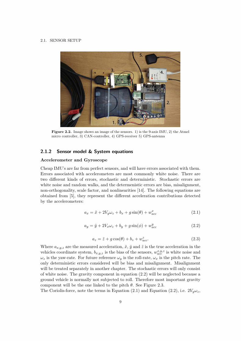
In the current control system of the latest generations of heavy duty vehicles, theTMS has a 2-axis IMU integrated in the control unit. It consists of 2 accelerom-eters oriented in the vehicles forward direction and to the side of the vehicle, hasthe capacity to send data with an update frequency of 100 Hz. The raw data fromthe GPS-signal is received with 5 Hz, the data is then transmitted over the internalCAN network such that the TMS can receive it, but only with 1 Hz. In Figure2.1 a simple schematics show how the signals are transferred through the network.Because the GPS have potential to provide a much higher update-frequency an ex-ternal GPS-receiver identical with the GPS in the vehicle was programmed suchthat it could transfer data at a higher frequency. It was connected directly to thecomputer through a serial port, and was transferred through a virtual CAN into thelogging software Vision. In Figure 2.1 the bottom part of the image, a simplifiedillustration of the sensor structure and how it is logged. The components used aredisplayed in Figure 2.2.

To investigate which gyros and accelerometers were necessary a nine-axis IMU waspurchased. 3 accelerometers, 3 gyros, and 3 magnetometers. Data was only col-lected from the accelerometers and Gyro-scopes, because the magnetometers willgive the direction globally to the magnetic poles and not necessary in determiningthe velocity of the vehicle. To interface the IMU such that it could be transmittedand stored over the CAN-network, a micro controller that was equipped with aCAN-controller, was borrowed from the Mechatronics department at KTH.

The virtual sensors (vSen) software currently used in the TMS to obtain an estimateof the vehicles speed is based on the wheel-encoder [1]. To compare this estimationto the estimation made by the proposed algorithms a very accurate reference-GPSwas borrowed. This reference GPS was connected directly to the computer and

7

CHAPTER 2. METHODS

logged in Vision. This can be seen in the lower part of Figure 2.2.

Computer

GPS TMS

VisionGPS

Ref. GPS

IMU6-axis

µ-controller

Serial to CAN

conversion

100 Hz

5 Hz

60 Hz

5 Hz

CAN

Virtual-CAN

CAN

Raw Data

Internal communication

CAN-network

Signal Processing

Raw Data

I2C

2.5 Hz

60 Hz

Raw Data

Serial

Raw Data

IMU2-axis

Raw Data

100 Hz

Current signal Path

1 Hz

Output-

Shaft100 Hz

Raw Data

Figure 2.1. Image shows how the signals from the IMU, Output-shaft and GPSarrives in the TMS control-unit. In the bottom of the image shows how the sensorsare interfaced and logged in vision.

8

2.1. SENSOR SETUP

Figure 2.2. Image shows an image of the sensors. 1) is the 9-axis IMU, 2) the Atmelmicro controller, 3) CAN-controller, 4) GPS-receiver 5) GPS-antenna

2.1.2 Sensor model & System equationsAccelerometer and Gyroscope

Cheap IMU’s are far from perfect sensors, and will have errors associated with them.Errors associated with accelerometers are most commonly white noise. There aretwo different kinds of errors, stochastic and deterministic. Stochastic errors arewhite noise and random walks, and the determenistic errors are bias, misalignment,non-orthogonality, scale factor, and nonlinearities [14]. The following equations areobtained from [5], they represent the different acceleration contributions detectedby the accelerometers:

ax = x+ 2Vyωz + bx + g sin(θ) + wxacc (2.1)

ay = y + 2Vxωz + by + g sin(φ) + wyacc (2.2)

az = z + g cos(θ) + bz + wzacc. (2.3)Where ax,y,z are the measured acceleration, x, y and z is the true acceleration in thevehicles coordinate system, bx,y,z is the bias of the sensors, wx,y,zacc is white noise andωz is the yaw-rate. For future reference ωy is the roll-rate, ωx is the pitch rate. Theonly deterministic errors considered will be bias and misalignment. Misalignmentwill be treated separately in another chapter. The stochastic errors will only consistof white noise. The gravity component in equation (2.2) will be neglected because aground vehicle is normally not subjected to roll. Therefore most important gravitycomponent will be the one linked to the pitch θ. See Figure 2.3.The Coriolis-force, note the terms in Equation (2.1) and Equation (2.2), i.e. 2Vyωz,

9

CHAPTER 2. METHODS

will be restricted. In land vehicle application, some rotations and velocities are lesslikely to occur. Velocities like Vz,y are restricted because the vehicle doesn’t slip orjump. But because the position of the IMU and GPS receiver would be located inthe centre of rotation. This is not the case, therefore this will be a source of errordue to the Coriolis effect. This error will only give a large error when the vehicle isturning rapidly. This phenomenon will be discussed in later sections.The gyro is not affected by gravity in the same way as the accelerometers, it will bemodelled to have a bias and noise. The following gyro-model is also obtained from[5].

gx,y,z = ωtruex,y,z + br + vgyro (2.4)

Where gx,y,z is the measured angular-rate ωx,y,z is the true angular-rate, and br isthe bias, and vgyro is zero mean white noise.

Figure 2.3. Image shows how the measurement is affected by gravity.

10

2.1. SENSOR SETUP

Global Positioning System

The GPS can provide velocity measurements in three dimensions, either in theearth-frame or the inertial frame. See Figure 2.4. It is very common that a GPScan send both depending on preference. In this project the velocity measurementswere sent in the earth frame. It is centered in the vehicle, and will provide thevelocity coordinates north-east-down (NED). These measurements can then be usedto obtain further information, such as the vehicles velocity, course, climb-rate andpitch. The following equations for pitch and velocity based on the GPS are obtainedfrom [5].

VGPS =√V 2north + V 2

east + V 2down (2.5)

θGPS = sin−1(VdownVGPS

)(2.6)

Where Equation (2.5) is the velocity of the vehicle, and Equation (2.6) is the Pitch.

Figure 2.4. Earth centred frame, and navigation frame (NED). The GPS sends itsmeasurements in the (NED) frame, green colors.

Equation (2.6) when VGPS is small or zero, the arc-sinus function is either infiniteor not defined. Resulting in a very inaccurate Pitch measurement. Thus the mea-surement will only be available after certain velocities. To illustrate this, the errorsmagnitude as a function of the vehicles velocity is showed in Figure 2.5. Indicatingthat the standard deviation tendes to infinity when the velocity approaches zero.[5]

σθGP S= σGPSdown

VGPS(2.7)

11

CHAPTER 2. METHODS

Figure 2.5. Illustrates the accuracy of the angles and how it changes with respectto the velocity. Image taken from [5]

.

Drive-line and output-shaft

The drive-line is a fundamental aspect of obtaining a good vehicular model. Thereare several ways to model a drive, and they vary with respect to their intended use.In Figure 2.6 there is a very basic model of drive-line with the most important com-ponents. Because the TMS is the control-unit for the transmission, there is a directmeasurement of the Output-shaft. The Output-shaft is connected to the propeller-shaft and because no friction between them is considered, it can be assumed that theOutput-shaft is equivalent to the propeller-shaft. The final drive is characterizedby a conversion ratio which equal is to a gear-ratio in the transmission[24]. Becausea very simple model assuming the drive-shaft and the wheels are a lumped-mass,together with the assumption that the two wheels rotate with an identical speed.The equation for how the Output-shaft relates to the velocity can be simplified toa single constant, see Equation (2.8). This holds true when the wheels have no slip.

V shaftx (k) = Csshaft(k) (2.8)

12

2.1. SENSOR SETUP

Engine Clutch

Transmission

Output Shaft

Wheel

Final Drive

Drive Shaft

Measurements available

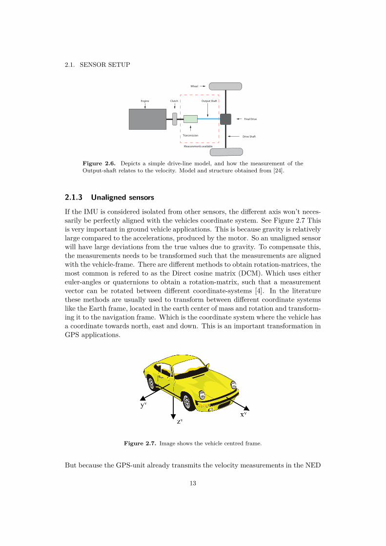
Figure 2.6. Depicts a simple drive-line model, and how the measurement of theOutput-shaft relates to the velocity. Model and structure obtained from [24].

2.1.3 Unaligned sensors

If the IMU is considered isolated from other sensors, the different axis won’t neces-sarily be perfectly aligned with the vehicles coordinate system. See Figure 2.7 Thisis very important in ground vehicle applications. This is because gravity is relativelylarge compared to the accelerations, produced by the motor. So an unaligned sensorwill have large deviations from the true values due to gravity. To compensate this,the measurements needs to be transformed such that the measurements are alignedwith the vehicle-frame. There are different methods to obtain rotation-matrices, themost common is refered to as the Direct cosine matrix (DCM). Which uses eithereuler-angles or quaternions to obtain a rotation-matrix, such that a measurementvector can be rotated between different coordinate-systems [4]. In the literaturethese methods are usually used to transform between different coordinate systemslike the Earth frame, located in the earth center of mass and rotation and transform-ing it to the navigation frame. Which is the coordinate system where the vehicle hasa coordinate towards north, east and down. This is an important transformation inGPS applications.

Figure 2.7. Image shows the vehicle centred frame.

But because the GPS-unit already transmits the velocity measurements in the NED

13

CHAPTER 2. METHODS

coordinate-system, it is not necessary to preform this transformation in this project.But the same equations can be used simply to rotate a vector to another arbitrarycoordinate system.The use of Euler angles have downsides, the most problematic is that there will besingularities when the inverse-sinus function is performed. A better method is tocalculate the direct cosine matrix using quaternions. It uses hyper complex variablesto calculate the rotation of a vector along another vector in three dimensions [15],

cos(θ) = v1 · v2 (2.9)

w = v1 × v2 =[w1 w2 w3

](2.10)

q =[cos( θ2) sin( θ2)w1 sin( θ2)w2 sin( θ2)w3

]= (2.11)

=[q1 q2 q3 q4

].

The first vector,v1 , would be the current IMU-measurement. The second vector,v2,is the vector the first one is rotated to, usually the direction of gravity. The thirdvector w is the vector in which v1 is rotated around with the angle θ. If thequaternion is normalized, the following rotational matrix can be constructed

R =

(q21 + q2

2 − q23 − q2

4) 2(q2q3 − q1q4) 2(q2q4 + q1q3)2(q2q3 + q1q4) (q2

1 − q22 + q3

1 − q24) 2(q3q4 − q1q2)

2(q2q4 − q1q3) 2(q3q4 + q1q2) (q21 + q2

2 − q23 − q2

4)

. (2.12)

Because of the IMU is strapped down, it will be fixed in the vehicle frame and veryunlikely that the orientation of the IMU will change relative the vehicle frame. It isa feasible assumption that the rotation matrix in Equation (2.12), will be constant.Thus this alignment step only need to be performed once on a flat surface, thensaved for future use.

ax,y,z = RaRawx,y,z, (2.13)ωx,y,z = RωRawx,y,z. (2.14)

14

2.2. STATE EQUATIONS

2.2 State equationsThe state equations should capture the most important dynamics of the vehicle.Because there is no knowledge of the input to the system, like the demand of torqueprovided by the driver. The state equations are only dependent on the dynamics ofthe acceleration. The most important states are the pitch and the velocity. Thusthere needs to be a state for both of them. Because the GPS will always be partof the sensor configuration, both the velocity and the pitch will be observable. Thegyro will be considered if it will improve the estimation or not. Thus there needsto be two different state equations. State equations considering a gyroscope,

x(k + 1) =

v(k + 1)a(k + 1)bv(k + 1)θ(k + 1)ω(k + 1)

=

v(k) + {a(k)− g sin(θ(k))}∆t− bv(k)

a(k)bv(k)

θ(k) + ω(k)∆tω(k)

(2.15)

y(k) = h(x) =

v(k)a(k)θ(k)ω(k)

=

1 0 0 0 00 1 0 0 00 0 0 1 00 0 0 0 1

x(k) = Hx(k). (2.16)

State equations that is not considering a gyroscope,

x(k + 1) =

v(k + 1)a(k + 1)bv(k + 1)θ(k + 1)

=

v(k) + {a(k)− g sin(θ(k))}∆t− bv(k)

a(k)bv(k)θ(k)

(2.17)

y(k) = h(x) =

1 0 0 00 1 0 00 0 0 1

x(k) = Hx(k). (2.18)

When there is a loss of a sensor like the GPS signal. The H matrix will be reducedsuch that only the accelerometer is available. This is done by setting the ones inthe rows of the h(x) function representing the velocity and road grate to zero. [25]

2.3 Kalman filterThe Kalman Filter is one of the most common state estimation filters. The linearKalman filter relies on linear state equation, it is also known as an optimal filter. Itwill be optimal if there is perfect information about the covariances of the system[2]. But in all real systems there are some nonlinearities, thus the need for anExtended Kalman-filter. It is generally good for sensor fusion application,and there

15

CHAPTER 2. METHODS

are a lot of literature of implementation of this filter. The following system is basedon [6][7],

xk+1 = fk(xk) + wk (2.19)yk = hk(xk) + vk (2.20)

where xk+1 is the discrete state vector, yk the output, wk is the noise in the plant,and vk is noise in the observation. Both are white Gaussian noise, with zero mean,and have the corresponding covariance matrices,

cov[vkv

tk

]= Rk (2.21)

cov[wke

tk

]= Qk. (2.22)

Q is the covariance matrix associated with the model and the input noise, and R thecovariance matrix of the measurement noise. The extended Kalman filter, is a firstorder filter. It linearise around the previous point to obtain an estimate about thenext one. The higher order dynamics are assumed to be zero. Note the extendedKalman filter is not optimal like its linear equivalent, due to linearisation.The extended Kalman filter can be separated into two phases, the prediction stepand the correction step. The prediction and correction is done recursively.

Prediction

Here the P is the error covariance matrix,

Pk|k = cov[xk − xk|k

](2.23)

xk+1|k = fk(xk+1|k) (2.24)Pk+1|k = FkPk|kF

Tk +Qk. (2.25)

Where Fk, and Hk+1 are the Jacobian of the state equation and the observation.

F (k) = ∂fk∂x|xk|k (2.26)

Hk+1 = ∂h

∂x|xk+1|k (2.27)

16

2.4. SLIDING MODE OBSERVER

Correction

K is the Kalman gain matrix.

Kk+1 = Pk+1|kHTk+1

[Hk+1Pk+1|kH

Tk+1 +Rk+1

]−1(2.28)

xk+1|k+1 = xk+1|k +Kk+1[yk+1 − hk+1xk+1|k

](2.29)

Pk+1|k+1 =[I −Kk+1Hk+1Pk+1|k

](2.30)

The Prediction and Correction set is repeated indefinitely.

2.4 Sliding mode observer

2.4.1 Non-linear Sliding mode observerThe Sliding mode observer will have similar structure as the Kalman filter, it canbe compared to the prediction and correction step. The main benefit of the SMOis that it doesn’t require any information of the covariances of the input signals orerrors. Thus very effective for non-linear systems that are sensitive to model-errors.Another big benefit of the SMO compared to the Kalman-filter, is that it doesn’tneed to re-compute the Kalman gain, Equation (2.29), or the error covariance ma-trix, Equation (2.30). The Kalman gain is especially hard to compute due to theinverse matrix operation, which is computationally demanding for large systems.The downside of the SMO is that if implemented poorly it will have non-linearchattering phenomenon. The SMO is based on Lyapunov theory and will guarenteeasymptotically convergence, if one can find a Lyapunov function. The chatteringphnomenon can be limited with a proper choise of the switching function [20]. Be-cause in this project the state equations will be nonlinear, there is a need for anonlinear filter. Core-ideas and assumptions are quite similar between the linearand the non-linear Sliding mode observer [19][22]. For the non-linear system.

xk+1 = fk(xk) +Bkuk + wk (2.31)yk = hk(xk) + vk. (2.32)

The following assumptions need to be considered,Assumption 1 the system is Bounded Input, Bounded States (BIBS).Assumption 2 the disturbances in the system are upper bounded [22].If these conditins are fullfilled the Sliding mode observer will take the form, [18].

xk+1|k = fk(xk−1) (2.33)yk = yk − h(xk−1) (2.34)

xk+1|k+1 = xk+1|k +Klineary −KSMOsat(yk/φ) (2.35)

17

CHAPTER 2. METHODS

Where the gain is split into a linear feedback gain Klinear, and one switching gainKSMO. To avoid the chattering phenomenon, that is usually a problem with theclassical Sliding mode observer, the switching sigmoid function can be replaced witha saturation function.

sat(yk, φ) ≡{yk/φ, |yk| ≤ φsign(yk) |yk| > φ

(2.36)

Where φ is the width of the boundary layer. From [22] stability is proven withLyapunov theory, and a lower and upper bound of the Sliding mode gain is pro-vided. But like [18] an averaged Kalman gain for Klinear for fast tuning will beimplemented.

2.5 Fusing two redundant signalsThe Output-shaft and the GPS will make two independent observations of thevelocity, and the true velocity is unknown. Therefore these two redundant mea-surement needs to be fused together. One method to fuse two redundant signals isthe weighted least square (WLS). It utilises the knowledge of the individual sensorscovariance and makes a weighted estimate[3].

x1 = x+ x1, cov(x1) = P1 (2.37)x2 = x+ x2, cov(x1) = P2 (2.38)P = (P−1

1 + P−12 )−1 (2.39)

x = P (P−11 x1 + P−1

2 x2) (2.40)

2.6 Testing, and Critical scenariosTo investigate the robustness of the proposed algorithms, data was collected fromcritical scenarios. At Scania Södertälje, there is a big test circuit that is constructedsuch that it replicates different scenarios a heavy-duty vehicle might encounter. Alarge variety of test-vehicles with different characteristics and performance are avail-able for testing. The test were performed on a vehicle with normal specifications,and flexibility to place the sensor such that it could be easily mounted. Becausethe large variability of circuit, the test-scenarios could be decided beforehand.

Hills

Hills are a critical scenario because the accelerometer is gravity-dependent as dis-cussed in Section 2.1.2. If the pitch is omitted the error occurring in the accelerom-eter will make the velocity drift away from the true velocity in a small time period.

18

2.6. TESTING, AND CRITICAL SCENARIOS

On Scanias test-circuit there are several hills, with inclinations up to a road grade of16%, or about 9o. Thus scenarios with both hills with large and small inclinationswill be evaluated.

Velocity extremes: Low- and High-speeds

Consider Figure 2.8, as indicated in the lower plot the wheel sensors will have anabsolute error at high velocities. This is a scale-factor error, mostly due to an errorin the estimation of the wheel’s radius. Thus this is a clear area of improvement.

0 0.5 1 1.5 2 2.5 3 3.5 4

0

0.5

1

1.5

2

time [s]

velo

city

[km

/h]

Wheel encoderReference GPS

465 470 475 480 485 490 495

80

85

90

velo

city

[km

/h]

time [s]

Wheel encoderReference GPS

Figure 2.8. Illustrates where the velocity from TMS based on the wheel encodershave poor accuracy. At low velocities the wheel-encoders will not provide a signalbefore ≈ 1m/s, showed in the top image. Due to a scale-factor error the wheelencoders will also have poor properties at high velocities, illustrated in the lowerimage.

Also indicated in Figure 2.8 in the top plot, the current method have issues at thelower velocity spectrum as well i.e. ≈ 0 − 1m/s. The wheel encoders will providea velocity signal after a certain threshold. Thus this scenario is most desirable forScania to improve.

Signal deterioration: slip and GPS outage

Because both the GPS and the Output-shaft have problems with reliability, becom-ing lost or bad, for example when the Output-shaft will start to slip, or the GPS islost due to driving inside a tunnel. Normally one signal can be complemented bythe other. But this doesn’t prevent the system from being bad all together, both

19

CHAPTER 2. METHODS

the GPS and Output-shaft are bad at the same time. Thus one critical scenariowould be if the entire velocity signal is lost and then investigate how the systembehaves.

2.7 Slip detectionThe Output-shaft will give a accurate velocity signal if scaled properly. But becausethe Output-shaft provides torque to the driving wheels, when the tiers loose frictionand starts to spin the signals accuracy will decrease. Thus it is very importantto have a good indication when the wheels start to spin. Because it was hard tosimulate wheel slip on the test-track. Data of slip was obtained from tests conductedat Scanias yearly tests in winter conditions. To obtain the slip such that it couldbe added artificially to other data, the true velocity was compared to the velocitysignal from the Output-shaft. The result is shown in Figure 2.9.

time [s]

0 10 20 30 40 50 60

velo

city [m

/s]

-1.5

-1

-0.5

0

0.5

1

1.5

2

2.5

3

Slip velocity ∆v

Figure 2.9. Image of the velocity difference between the actual velocity and thevelocity measured by the Output-shaft. Obtained from a winter-scenario where avehicle slips due to poor friction.

To obtain a good indication when the Output-shaft was slipping, it is usually agood idea to look at the signals derivatives. It will reveal high frequency changeslike oscillations. But derivatives of an already noisy signal is also noisy. Thus isnot suitable to quantify an answer whether the signal is good or not. One solutionmight be to investigate the energy of the signal. Because most signals don’t havefinite energy it is interesting to look at a signals energy during finite time [2]. Thisalso saves a lot of computational effort saving data from a short period prior. This

20

2.8. LATENCY COMPENSATION

might reveal some information of the slip in the signal. Thus one might look at theRMS during a short period of time.

RMS(x) =√

1N

(x21 + x2

2 + . . .+ x2n) (2.41)

But as Figure 2.9 indicates there are low frequency components in the slip, and theRMS will be good at detecting high frequency content. The variance of the signalwas proven to be a better indicator.

V ar(x) = 1N

N∑k=1

(xk − µ) (2.42)

Where µ is the average.To quantify when the Output-shaft is bad, different logical conditions will make adecision to trust the Output-shaft or not. The first flag will indicate if the Output-shaft is slipping and the second flag will indicate if there is a velocity differencebetween the GPS and Output-shaft, and the third flag will indicate if the vehicleis turning very rapidly. These three flags will realize which of the Output-shaft orthe GPS is deviating from the true velocity.

2.8 Latency compensation

In real systems there will always be latency associated with the implementation.The GPS will have more latency compared to the Output-shaft or the accelerom-eter. This is because the signal needs to be processed and converted, and in theprocess creating latency. Because the computational effort will be somewhat con-stant, the delay will also be constant. Which simplifies the problem considerably.There are several ways to handle measurement delay. The easiest and the mostinaccurate is to ignore that there are delay. This will be the most computationalefficient. Another method is to re-calculate the entire time-trejectory. This will bevery demanding both storagewise and computationally, and grows larger the longerthe time delay[17].

The Latency compensation method with the Kalman filter is in accordance with themethod described in [16], and is refered to as Larsens method in [17]. The principleis that you have two parallel filters, one that calculates the state estimation whenthe measurement arrives, as if there was no delay. The other filter starts at timel = k − N , where N is the number of samples the delay represent, and uses thecovariance R∗k. Up until the time k, the estimates from the first filter will be used.But when the delayed measurement arrives, the measurement will be fused in theparallel filter. The measurement vector is then extrapolated.

21

CHAPTER 2. METHODS

yintk = y∗k +H∗k xk −H∗l xl (2.43)

where l = k − N and N is the number of samples the delay represents. y∗k is thenon-delayed measurement. Through N succeeding time data updates from time l tok, the estimation error covariance therefore becomes:

M = E{xlxTk } = Ps

N−1∏i=0

ATk−i−1(I −Kk−iHk−i)T (2.44)

M∗ =N−1∏i=0

(I −Kk−iHk−i)Ak−i−1 (2.45)

The new updated Kalman gain.

Kk = M∗PlH∗Tl [C∗l PlH∗Tl +R∗k]−1 (2.46)

Updating the covariance matrix of the error.

Pk+1|k = Pk|k −KkH∗l PlM

T∗ (2.47)

Then if adding the following expression after yk has been fused.

δxk = M∗Kl(y∗k −H∗l xl) (2.48)

Adding this extra filter will naturally increase the computational load.This idea can translate to the Sliding mode observer. Extrapolate the measurementusing equation 2.43, then using the measurement update step equation 2.35 to obtainxl with the correct non-lagged measurement. The extrapolated measurement willthen be fused in the in the filter normally. But this method is suboptimal[17].

22

Chapter 3

Results

3.1 General characteristics of the signals, and results

3.1.1 GPSAs mentioned in Section 2.8, the GPS-measurement will be delayed. This is il-lustrated in Figure 3.1, where the GPS signal is shown together with the highlyaccurate reference GPS. The raw GPS-signal has a constant delay of 500ms. If thesignal if shifted 0.5s backwards in time the GPS-signal will accurately follow thereference GPS. When comparing the raw GPS-signal with the original GPS signalwith 1Hz from the CAN-network, the GPS only has a delay of 250ms. This is mostlikely due to suboptimal sensor-architecture and interfacing. This will be a futurearea of improvement. But if the interfacing was optimised, one might expect toreduce the delay at least to match the level that is currently in the TMS. Thereforeit is justified to shift the signal such that there is only a delay of 250 ms in the GPS-measurement. This will make the comparison between the current wheel-encoder(WE) estimate and the proposed methods more comparable.

23

CHAPTER 3. RESULTS

time [s]

8 9 10 11 12 13

velo

city [m

/s]

0

2

4

6

original

GPS-signal

ref-GPS

time [s]

8 9 10 11 12 13

velo

city [m

/s]

0

2

4

6

offset ≈ 0.5s

GPS-signal

ref-GPS

Figure 3.1. The top figure the raw GPS-signal is shown together with referenceGPS. In the lower image the same signal is shifted 0.5 s in time. The shifted signalfollows the reference accurately.

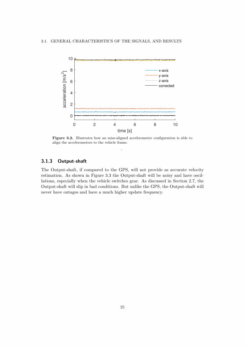
3.1.2 Alignment of strap-down IMUIn Section 2.1.3, a misalignment of the strap-down IMU was discussed together witha method to compensate for it. As shown in Figure 3.2 the misaligned IMU can becentred to the vehicle frame. This is done such that it is aligned along the directionof gravity. This requires that there is no accelerations other than gravity. Thiswould require that the vehicle is on a flat surface when the algorithm is performed,otherwise the IMU will not be aligned properly. But because it is unlikely thatthe strap-down IMU change its orientation relative the vehicle frame, the rotationmatrix will remain constant. Thus by saving a matrix from a scenario where thevehicle is on a flat surface, the matrix can be reused. The alignment step can beperformed again to align the IMU in the xy-plane. This would require that there isa clear signal of an acceleration in the forward direction.

24

3.1. GENERAL CHARACTERISTICS OF THE SIGNALS, AND RESULTS

time [s]

0 2 4 6 8 10

accele

ration [m

/s2]

0

2

4

6

8

10

x-axis

y-axis

z-axis

corrected

Figure 3.2. Illustrates how an miss-aligned accelerometer configuration is able toalign the accelerometers to the vehicle frame.

.

3.1.3 Output-shaftThe Output-shaft, if compared to the GPS, will not provide as accurate velocityestimation. As shown in Figure 3.3 the Output-shaft will be noisy and have oscil-lations, especially when the vehicle switches gear. As discussed in Section 2.7, theOutput-shaft will slip in bad conditions. But unlike the GPS, the Output-shaft willnever have outages and have a much higher update frequency.

25

CHAPTER 3. RESULTS

Time [s]

7 8 9 10 11 12 13 14

Velo

city [m

/s]

0

1

2

3

4

5

6

vShaft

vRef

Figure 3.3. Image shows the typical Output-shaft signal, when scaled properly. Inthe image one can clearly see gear switching, time 10.5[s], which will make the signaloscillate.

3.2 Comparison Kalman vs. Sliding modeIn this section the difference between the Sliding mode observer (SMO), ExtendedKalman filter (EKF), and the current TMS wheel encoder based velocity estima-tion from Scania is explored (TMSWEE). In the tables the root mean square error(RMSE), mean absolute error(MAE), and the peak error or the largest error occur-ring in this sequence are displayed. Two different scenarios was used to illustratethe differences. A small hill, making the pitch an important state to estimate. Alonger scenario with high speeds, fast accelerations and to investigate the overallperformance of the filters.

Small hill

In Figure 3.4 the result from the two different filters are displayed, and the result-ing error-analysis is shown in Table 3.1. Both the EKF and the SMO have bet-ter performance than the TMSWEE in both the root-mean-square error (RMSE)and mean-absolute error (MAE). If one investigates the figure this is occurringwhen the vehicle is de-accelerates rapidly. Thus the large amplitude error is dueto the fact that the GPS is delayed and the entire signal will have an offset.

26

3.2. COMPARISON KALMAN VS. SLIDING MODE

Kalman Filter Sliding mode Observer TMSWEE

RMSE 0.5742 0.5652 0.7062MAE 0.4571 0.4484 0.5996Peak Error 1.5370 1.5178 1.4040

Table 3.1. Comparison of the Extended Kalman Filter, the Sliding mode observer,and the current method from the TMS based on wheel encoders (TMSWEE). Thisis from the scenario where the vehicle is driving up a small hill.

time [s]

5 10 15 20 25 30 35 40

|∆v| [k

m/h

]

0

1

2Absolute Error

Kalman|

SMO|

TMSWEE|

time [s]

28 29 30 31 32 33 34 35 36 37 38 39

velo

city [km

/h]

18

22

26

Velocity

vKalman

vSMO

vTMSWEE

vRef

time [s]

5 10 15 20 25 30 35 40

Pitch [ra

d]

-0.2

-0.1

0

0.1Pitch θ

Kalman

θSMO

θTMSWEE

Figure 3.4. This picture shows a drive-scenario from a small hill. In the top imagethe absolute error in the estimated velocity compared to the reference GPS’s "truevelocity" is displayed. In the middle image displays the velocity-estimation from theSMO and Kalman, together with the reference GPS and the TMSWEE. The imageis also zoomed in on the velocity when the vehicle is driving over the hill. In thebottom image the pitch is displayed.

27

CHAPTER 3. RESULTS

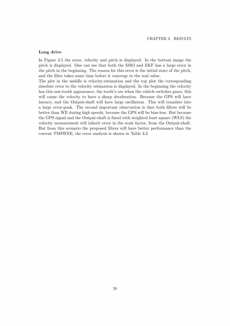
Long drive

In Figure 3.5 the error, velocity and pitch is displayed. In the bottom image thepitch is displayed. One can see that both the SMO and EKF has a large error inthe pitch in the beginning. The reason for this error is the initial state of the pitch,and the filter takes some time before it converge to the real value.The plot in the middle is velocity-estimation and the top plot the correspondingabsolute error to the velocity estimation is displayed. In the beginning the velocityhas this saw-tooth appearance, the tooth’s are when the vehicle switches gears, thiswill cause the velocity to have a sharp deceleration. Because the GPS will havelatency, and the Output-shaft will have large oscillation. This will translate intoa large error-peak. The second important observation is that both filters will bebetter than WE during high speeds, because the GPS will be bias-less. But becausethe GPS signal and the Output-shaft is fused with weighted least square (WLS) thevelocity measurement will inherit error in the scale factor, from the Output-shaft.But from this scenario the proposed filters will have better performance than thecurrent TMSWEE, the error analysis is shown in Table 3.2.

28

3.2. COMPARISON KALMAN VS. SLIDING MODE

time [s]

320 340 360 380 400 420 440 460 480 500

|∆v| [k

m/h

]

0

1

2

3Absolute Error

Kalman|

SMO|

TMSWEE|

time [s]

320 340 360 380 400 420 440 460 480 500

ve

locity [

km

/h]

0

20

40

60

80

Velocity

vKalman

vSMO

vTMSWEE

vRef

time [s]

320 340 360 380 400 420 440 460 480 500

Pitch

[ra

d]

-0.1

0

0.1

0.2Pitch

θKalman

θSMO

θTMSWEE

Figure 3.5. This image displays a longer driving-scenario when the vehicle is sub-jected to fast accelerations, and both low- and high-velocities. In the top image theabsolute error in the estimated velocity compared to the reference GPS’s "true veloc-ity" is displayed. In the middle image displays the velocity-estimation from the SMOand Kalman, together with the reference GPS and the TMSWEE. In the bottomimage the pitch is displayed.

Kalman Filter Sliding mode Observer TMSWEE

RMSE 0.8509 0.8468 1.5822MAE 0.7441 0.7416 1.3696Peak Error 2.7772 2.7122 3.6360

Table 3.2. Comparison of the Extended Kalman Filter, the Sliding mode observer,and the current TMSWEE. This is from the case where the vehicle is a case wherethere is a longer drive with both hills, high- and low-velocities.

29

CHAPTER 3. RESULTS

3.3 Improving the sensor configurationTo evaluate if there are any benefits in having a more complete sensor-configuration,a gyro was added to the state equation to provide an observation on the pitch’sangular-velocity. This was then compared to the sensor-configuration that resembleswhat is currently available from the TMS. The reference-GPS bases its estimationon an IMU with very high quality and a GPS. These raw-signals are available. Theaccelerometers in from the IMU used in this project had relative good accuracy, butthe gyroscope’s was not. Therefore to investigate how a much better the estimatebecomes with an accurate IMU, the gyroscope measurements from the reference-GPS will be used, then compared to the normal gyro.

Another area where a more complete sensor-configuration is beneficial is in thecase when the vehicle is subjected to a sharp turn. Because the GPS-receiver willnot be in the centre of rotation, the GPS will measure slip-velocity. That is thevelocity around the centre of rotation. Because the vehicle is also turning theCoriolis effect, Equation 2.1, will make the x-axis accelerometer inaccurate. Butbecause the Output-shaft does not measure this slip of the GPS, the velocity dif-ference will be the slip velocity of the GPS. If one adds a yaw-gyroscope ωz, thusthe Coriolis-acceleration is observable and its error on ax can be compensated for.

Pitch-gyro

In Table 3.3 the two different models were evaluated when the Output-shaft wasavailable. Both estimations are accurate considering difference in the RMSE andMAE between the two filters.

In the case where the Output-shaft is omitted, the need for a gyro becomes moreapparent. This is displayed in Table 3.4. The filters were evaluated when thevelocity and pitch measurement was limited to only the GPS-signal and IMU. Wherethe pitch have rapid changes, the gyro-less system will have inaccurate informationof the pitch in between the GPS-samples due to the slow update-frequency of theGPS. Resulting in an inaccurate gravity compensation on the accelerometer. Thevelocity estimation will therefore have a peaky appearance between the GPS samplesand then jump back when the GPS-signal arrives. This will make the overall RMSEand MAE increase, compared to the setup with a rate gyro.

30

3.3. IMPROVING THE SENSOR CONFIGURATION

Without Gyro With gyro TMSWEE

RMSE 0.5762 0.5756 0.7062MAE 0.4572 0.4580 0.5996Peak Error 1.5721 1.5372 1.4040

Table 3.3. This table shows a summary of errors comparing the benefits of adding arate-gyroscope and not having a rate-gyroscope, when the Output-shaft is available.

Without Gyro With gyro TMSWEE

RMSE 0.6271 0.5115 0.7062MAE 0.5078 0.4187 0.5996Peak Error 1.7827 1.4219 1.4040

Table 3.4. This table shows a summary of errors comparing the benefits of addinga rate-gyroscope and not having a rate-gyroscope, when the Output-shaft is notavailable.

31

CHAPTER 3. RESULTS

A better Gyroscope

Here the scenario where the vehicle is driving in a small hill was considered. Ata critical point in the scenario where the pitch will change rapidly, all the signalsthat provides a velocity estimation was removed such that the system had to relysolely on the IMU. In Figure 3.6, the resulting pitch estimation is illustrated. Inthe bottom figure the normal gyroscope is used. It will start to deviate rapidlyafter 5 seconds. The accurate IMU from the reference GPS will however have amuch more accurate pitch estimation. In Figure 3.7 the corresponding velocity isshown. The estimation with the normal gyroscope will diverge rapidly compared tothe estimation with the better gyroscope.

time [s]

20 25 30 35 40 45

θ(k

) [r

ad

]

-0.2

-0.1

0

0.1Better gyro GPSout

θEst

θTMSWEE

time [s]

20 25 30 35 40 45

θ(k

) [r

ad

]

-0.2

-0.1

0

0.1

0.2Normal gyro

GPSout

θEst

θTMSWEE

Figure 3.6. Image shows the improvement of the estimation of the pitch with abetter gyroscope. During a simulated complete blackout of the velocity measurement,loosing both the GPS and Output-shaft signal.

32

3.3. IMPROVING THE SENSOR CONFIGURATION

time [s]

20 25 30 35 40 45

ve

loci

ty [

km/h

]

10

15

20

25

30Better gyro

GPS out

vTMSWEE

vEst

vGPS

vRef

vshaft

time [s]

20 25 30 35 40 45

ve

loci

ty [

km/h

]

-10

0

10

20

30Normal gyro

GPS out

vTMSWEE

vEst

vGPS

vRef

vshaft

Figure 3.7. Image shows the improvement of the estimation of the velocity with abetter gyroscope. During a simulated complete blackout of the velocity measurement,loosing both the GPS and Output-shaft signal.

3.3.1 CoriolisIn Figure 3.8, the velocity measured by the GPS, from the scenario where thevehicle is turning rapidly on a flat surface. The Output-shaft is displayed in thebottom figure. There is a clear velocity difference at two time intervals 10 − 20sand 80 − 95s. Similar velocity differences are observed in the velocity from theTMSWEE. The reason for this is that the GPS is not located in the centre ofrotation. So when the vehicle is turning the GPS is also measuring a velocityaround the centre of rotation together with the true-velocity. The same goes for thevelocity estimation from the TMSWEE, because the wheel encoders are located inthe front-wheels. For clarification see A.2. In the top figure the y-axis accelerometersoutput is displayed together with the calculated Coriolis-effect, aCoriolis. It wascalculated by multiplying the velocity difference between the Output-shaft and theGPS-measurement, multiplied by the yaw angular-velocity,

aCoriolis = (vGPS − vShaft)ωz. (3.1)

The yaw angular-velocity displayed in the middle figure.Because of this error in the velocity-measurement, it is desirable to omit the GPS-measurement during these instances where the Coriolis is present. Consider Section2.7 where the slip detection algorithm was described. It is important to flag whenthe GPS is un-trustworthy and when the Output-shaft is slipping. Thus the Coriolis-effect would be the ultimate indicator for when the GPS needs to be ignored. But

33

CHAPTER 3. RESULTS

one needs a minimum of 3 sensors to calculate the Coriolis: Output-shaft,GPS andgyro. The latter is not available in the current generation of TMS. Therefore analternative method to detect slip-velocity is needed.

If the acceleration ay is considered in isolation, it will contain the centrifugal accel-eration, and the acceleration that is producing the slip-velocity. Because there isone known and there are two unknowns, it is impossible to extract either.Consider the middle and top plot in Figure 3.8, ωz and ay will have a very similarappearance. So if the acceleration in the y-direction is large and there is a velocitydifference between the GPS and Output-shaft, the GPS is most likely subjected toslip. Thus for the purpose of indicating when there is slip, the y-acceleration canreplace Coriolis.

time [s]

20 40 60 80 100 120

ve

locity [

m/s

2]

-1

0

1V

yω

z

ay(k)

time [s]

20 40 60 80 100 120

[ra

d/s

]

-0.2

0

0.2

0.4

ωz

time [s]

20 40 60 80 100 120

ve

locity [

km

/h]

0

10

20

30vGPS

vShaft

vRef

Figure 3.8. The top figure shows the Coriolis-effect compared to the measuredacceleration on the y-axis. In the middle image the yaw-rate is displayed, and in thebottom image velocity from the Output-shaft and the GPS is compared. There is alarge velocity difference during sharp turns.

To illustrate how much the Coriolis-effect will impact the velocity estimation, thetop image in Figure 3.9 shows the calculated Coriolis-acceleration. In the middleimage the accelerometer measurements are simply integrated to obtain the velocity,together with the true velocity. In the bottom image the acceleration measured is

34

3.3. IMPROVING THE SENSOR CONFIGURATION

displayed together with the Coriolis corrected acceleration.If the Coriolis-acceleration is removed from ax the velocity estimate will be closerto the true-velocity of the vehicle. As the image indicate the Coriolis correctedaccelerometer will start to drift after about 40s compared to 5s from the uncom-pensated.

time [s]

20 40 60 80 100 120

[m/s

2]

-0.2

0

0.2

0.4

0.6Coriolis

Vyω

z

time [s]

20 40 60 80 100 120

[km

/h]

-20

0

20

Velocityv

xcorr

vx

vxref

time [s]

20 40 60 80 100 120

[m/s

2]

-2

-1

0

1

2Accelerometer

axcorr

ax

Figure 3.9. Image shows the benefits of compensating for Coriolis-accelerationsfor the measurements. In the top plot the Coriolis-acceleration in the x-direction isdisplayed. In the middle image the velocity from integrating the acceleration mea-surement, before and after compensating for Coriolis together with the true velocityis displayed. In the bottom plot the measurement of the acceleration is displayedbefore and after compensating for Coriolis.

.

35

CHAPTER 3. RESULTS

3.4 RobustnessIn this section the robustness of the estimations is considered. What would happenif a signal was lost or considered bad, for example the GPS is lost if there is a badreception, in a tunnel or in a City with high buildings.The Output-shaft will provide an accurate velocity estimation with high frequency,but the Output-shaft have some big issues in robustness. Especially in bad condi-tions, when the wheels looses grip. In Section 2.7 a method for detecting this slipwas proposed.Then the algorithm will be evaluated such that it preforms in both high and lowvelocities.

3.4.1 GPS-outageBecause Scanias test-circuit is outside, and no tunnels are available, the GPS-outagehad to be added artificially. To simulate this behaviour, the GPS signal was con-sidered as completely lost with no transition phase of deteriorating accuracy, likegoing into a tunnel. Two sensor-configurations are interesting to evaluate during aGPS-outage: with and without an Output-shaft signal.

If there is no Output-shaft observation the system needs to rely solely on the IMUto provide a estimate. As discussed in Section 3.3, it is important to have accurateIMU-sensors to maintain an accurate estimation during this outage period. Oth-erwise the system will have similar behaviour to Figure 3.7, and diverge from thetrue velocity rapidly.If there is an observation of the Output-shaft and the GPS, the system will be morereliable. The system will be vulnerable to errors in the Output-shaft observation,but it will be better than the previous scenario. The result of a GPS-outage withobservation of the Output-shaft is displayed in Figure 3.10. In the top of the figurethe absolute error is displayed. The proposed method without the GPS will outpreform TMSWEE during the period of the outage. The corresponding velocityprofile is displayed in the image below.

36

3.4. ROBUSTNESS

time [s]

20 22 24 26 28 30 32 34 36 38 400

0.1

0.2

0.3

0.4Absolute Error

|v ref -vest |

|v ref -vTMSWEE|

time [s]

20 22 24 26 28 30 32 34 36 38 40

ve

loci

ty [

km/h

]

10

15

20

25

30Velocity vTMSWEE

vEst

vGPS

vRef

vshaft

outageGPS

Figure 3.10. Illustrates the velocity estimation when the GPS has an outage. Be-cause the Output-shaft is still available the signal remains more accurate than TM-SWEE. But when compared to the fused GPS and Output-shaft, the estimationbecomes slightly more noisy.

3.4.2 Slip DetectionIn Figure 3.11 the signals used to indicate slip in both the Output-shaft and GPSis showed. The thresholds are indicated with a straight line, and black lines areindicating when the algorithm flags for a possible slip-scenario. Three differentflags were constructed to quantify when a signal might be bad.

• Flag 1: There is a velocity difference between the GPS and Output-shaft.

• Flag 2: The variance in the Output-shaft during the last N samples is high.

• Flag 3: The magnitude of the acceleration in the y-direction is high.

The bottom image shows the decision made by the algorithm, where the differentlevels illustrates the actual decision. There are 3 different decisions:

• All sensors are good

• Trust IMU and GPS, Flag 1 and Flag 2 is active.

• Trust IMU and Output-shaft, Flag 1 and Flag 3 is active.

The sharp turning driving-scenario was chosen, because it has areas where the GPSwill also have slip. So the algorithm has to differentiate between when the GPS is

37

CHAPTER 3. RESULTS

bad and when the Output-shaft is bad. See A.1 for a pseudo flow-diagram of thealgorithm.

0 20 40 60 80 100 120

1

2

flag3a

y(k)2

bhigh

blow

Flag

0 20 40 60 80 100 120

0.05

0.1flag2

var(vShaft)2

bhigh

blow

Flag

0 20 40 60 80 100 120

∆v

2

0

1

2flag1

(vGPS-vShaft)2

b

Flag

20 40 60 80 100 120

1

2

3

decision

Good

IMU+GPS

IMU+Shaft

Figure 3.11. Shows how the signals used to make a logical decision whether to trusta velocity measurement. Three different flags are used, and atleast two are needed tomake a deduction that the signal is either slipping or drifted.

In Figure 3.12 the velocity estimation from the algorithm is shown together with thevelocity measurements. The error between the estimated velocity from the proposedalgorithm and the "true" velocity from the reference GPS is shown. Slip was alsoadded afterwards during a period where the GPS was good, because otherwise it isobvious that the velocity estimation will be bad.

38

3.4. ROBUSTNESS

time [s]

0 20 40 60 80 100 120 140

|∆v

| [km

/h]

0

1

2

3Absolute Error

Est |

TMSWEE|

time [s]

0 20 40 60 80 100 120 140

ve

loci

ty [

km/h

]

0

10

20

30

Velocity

vTMSWEE

vEst

vGPS

vRef

vShaft

Slip

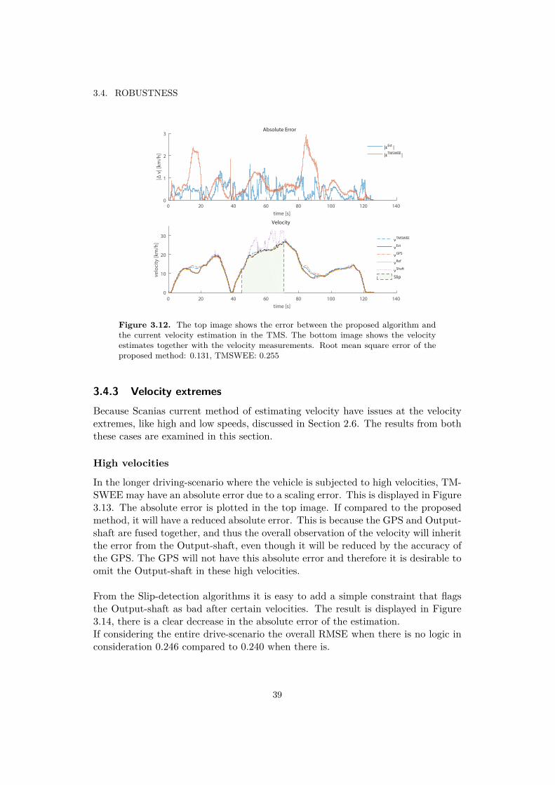
Figure 3.12. The top image shows the error between the proposed algorithm andthe current velocity estimation in the TMS. The bottom image shows the velocityestimates together with the velocity measurements. Root mean square error of theproposed method: 0.131, TMSWEE: 0.255

3.4.3 Velocity extremesBecause Scanias current method of estimating velocity have issues at the velocityextremes, like high and low speeds, discussed in Section 2.6. The results from boththese cases are examined in this section.

High velocities

In the longer driving-scenario where the vehicle is subjected to high velocities, TM-SWEE may have an absolute error due to a scaling error. This is displayed in Figure3.13. The absolute error is plotted in the top image. If compared to the proposedmethod, it will have a reduced absolute error. This is because the GPS and Output-shaft are fused together, and thus the overall observation of the velocity will inheritthe error from the Output-shaft, even though it will be reduced by the accuracy ofthe GPS. The GPS will not have this absolute error and therefore it is desirable toomit the Output-shaft in these high velocities.

From the Slip-detection algorithms it is easy to add a simple constraint that flagsthe Output-shaft as bad after certain velocities. The result is displayed in Figure3.14, there is a clear decrease in the absolute error of the estimation.If considering the entire drive-scenario the overall RMSE when there is no logic inconsideration 0.246 compared to 0.240 when there is.

39

CHAPTER 3. RESULTS

time [s]

450 460 470 480 490 500 510

|∆v

| [k

m/h

]

0

1

2

3Absolute Error

|v ref -vest |

|v ref -vTMSWEE |

time [s]

450 460 470 480 490 500 510

ve

loci

ty [

km/h

]

60

70

80

90Velocity

vTMSWEE

vEst

vGPS

vRef

vshaft

Figure 3.13. Top figure contains the absolute error of the proposed method andthe current TMSWEE. In the lower image the corresponding velocity-estimate isdisplayed.

time [s]

450 460 470 480 490 500 510

|∆v

| [k

m/h

]

0

1

2

3Absolute Error

|v ref -vest |

|v ref -vTMSWEE |

time [s]

450 460 470 480 490 500 510

ve

loci

ty [

km/h

]

60

70

80

90Velocity

vTMSWEE

vEst

vGPS

vRef

vshaft

Figure 3.14. Top figure contains the absolute error of the proposed method andthe TMSWEE. In the lower image the corresponding velocity-estimate is displayed.At fast speeds the Output-shaft will have bad properties due to errors in the scalefactor. Because both the GPS and the Output-shaft are accessible one can use a logicconstraint to only trust the GPS, thus improving the result.

40

3.4. ROBUSTNESS

Low velocities

Low velocities are a very critical scenario when a good estimation is desirable. Be-cause the TMS’s velocity estimation is based on the wheel encoders, and have ahysteresis property in this velocity spectrum. Therefore it will not provide a veloc-ity observation after a certain velocity. In Figure 3.15 in the top image the erroris displayed. The absolute error is growing until it hits about 1km/h before de-creasing. In the same image the error corresponding to the proposed method isdisplayed. It shows better performance than the TMSWEE in the lower regionsfrom about 0− 2km/h then the estimation deteriorates because of the delay in theGPS signal.

With the same reasoning for the high velocity case, the GPS will have bad propertiesin the lower velocity region. It is too slow and the delay will make the relative errorvery large. Therefore, ignoring the GPS at lower velocities will make the overallestimate better. In Figure 3.16 the error with only the velocity-observation fromthe Output-shaft and the acceleration from the IMU is used.The error is much smaller compared to the error from when both the GPS andOutput-shaft was used. But the TMSWEE out-preforms the proposed methodafter 2km/h to about 15km/h, because the wheel encoders are very accurate inthat region. Consider the previous figures for that velocity region. The error in thevelocity estimation from the proposed method is below 0.5km/h throughout thatregion.

time [s]

309 309.5 310 310.5 311 311.5 312

|∆v

| [k

m/h

]

0

0.5

1

Absolute Error

|v ref -vest |

|v ref -vTMSWEE |

time [s]

309 309.5 310 310.5 311 311.5 312

ve

loci

ty [

km/h

]

0

2

4

6Velocity

vTMSWEE

vEst

vGPS

vRef

Figure 3.15. Top figure contains the absolute error of the proposed method andthe current TMSWEE. In the lower image the corresponding velocity-estimate isdisplayed.

41

CHAPTER 3. RESULTS

time [s]

309 309.5 310 310.5 311 311.5 312

|∆v

| [k

m/h

]

0

0.5

1

Absolute Error

|v ref -vest |

|v ref -vTMSWEE |

time [s]

309 309.5 310 310.5 311 311.5 312

ve

loci

ty [

km/h

]

0

2

4

6Velocity

vTMSWEE

vEst

vGPS

vRef

Figure 3.16. Top figure contains the absolute error of the proposed method andthe current, TMSWEE. In the lower image the corresponding velocity-estimate isdisplayed. At low speeds the GPS will have bad properties due to latency and lowupdate-frequency. Because the GPS and the Output-shaft are fused together, thefused signal will inherit the delay and therefore have an offset to the true velocity.One can use a logic constraint to only trust the Output-shaft, thus improving theresult.

42

3.5. DELAY COMPENSATION

3.5 Delay compensationThe delay in the GPS is a serious problem in critical scenarios, low velocities seeSection 3.4.3, fast accelerations or deceleration. This leads to rapid deterioration ofthe estimations accuracy. To obtain accurate estimation with a sensor-configurationwith IMU and GPS this will be a big issue. One can either improve the sensor ar-chitecture and limit the magnitude of the delay. The other option is to compensatefor the delay. In Section 2.8 a method for compensating for the delay was proposed.

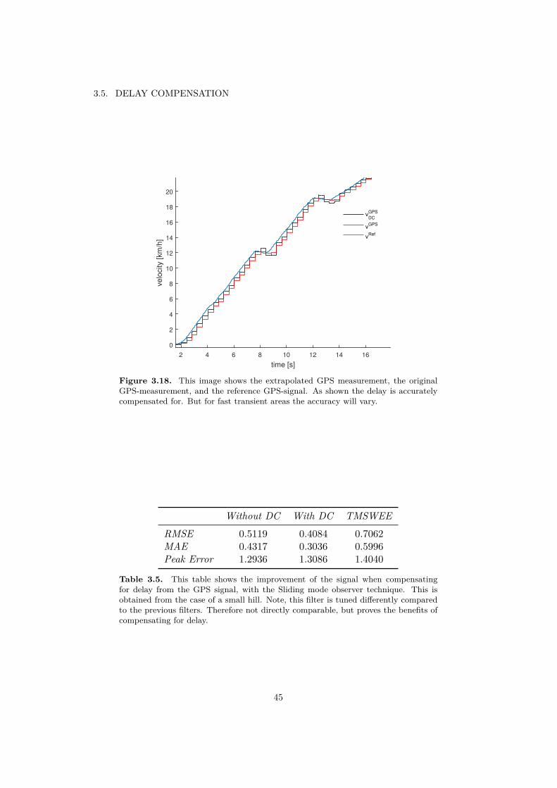
In Figure 3.17 the resulting velocity estimation is displayed. In the top imagethe absolute error between the reference GPS and the corresponding estimates arepresented. In the figure a segment of the drive-scenario is presented. From the topfigure it is clear that the delay compensation will overall have a lower absolute errorcompared to both the TMSWEE and the non-compensated.Because the method is based on measurement extrapolation, the correspondingmeasurement of the GPS-signal is displayed for a small segment of the scenario inFigure 3.18. In Table 3.5 a compilation of the errors from the scenario is displayed.There is a great improvement in both the RMSE and the MAE, compared to thenon-compensated system. The downsides are that in some cases the extrapolationtend to overshoot, thus making the peak error larger than the filter without delay-compensation.

43

CHAPTER 3. RESULTS

time [s]

0 5 10 15 20 25 30 35 40 45

|∆v

| [km

/h]

0

0.5

1

1.5Absolute Error no DC

|DC

|TMSWEE

|

time [s]

2 3 4 5 6 7 8 9 10

ve

loci

ty [

km/h

]

0

5

10

15

Velocity

vNo DC

vDC

vTMSWEE

vRef

Figure 3.17. This image shows the velocity estimation from the driving-scenariowhere the vehicle is driving up a small hill. To illustrate the improvement of com-pensating for the latency in the GPS, the Output-shaft is excluded. In the top plotthe absolute error from the velocity estimation from the SMO when latency is andis not compensated for. Together with the absolute error from the current TMS’sestimation.

44

3.5. DELAY COMPENSATION

time [s]

2 4 6 8 10 12 14 16

velo

city [km

/h]

0

2

4

6

8

10

12

14

16

18

20

vGPS

DC

vGPS

vRef

Figure 3.18. This image shows the extrapolated GPS measurement, the originalGPS-measurement, and the reference GPS-signal. As shown the delay is accuratelycompensated for. But for fast transient areas the accuracy will vary.

Without DC With DC TMSWEE

RMSE 0.5119 0.4084 0.7062MAE 0.4317 0.3036 0.5996Peak Error 1.2936 1.3086 1.4040

Table 3.5. This table shows the improvement of the signal when compensatingfor delay from the GPS signal, with the Sliding mode observer technique. This isobtained from the case of a small hill. Note, this filter is tuned differently comparedto the previous filters. Therefore not directly comparable, but proves the benefits ofcompensating for delay.

45

Chapter 4

Discussion and Conclusion

4.1 Discussion

Complete sensor configuration

The benefits of having a more complete IMU set-up is that the measurements ofthe pitch will have a more accurate and high-frequent update. This is importantwhen there is only a IMU+GPS configuration. This configuration is very importantbecause when the Output-shaft starts to slip, IMU+GPS will be the sensors thatwill provide the velocity estimate. Therefore it is important that the IMU measure-ments are accurate in-between the GPS samples. See Section 3.3 and Table 3.4.But if the Output-shaft is available as an additional velocity-observation, the over-all velocity-estimate will not be as dependent on a good acceleration measurement.Thus the performance will not be greatly impacted, therefore adding a pitch gyroto the TMS is not truly justified. See Figure 3.10.But when GPS-outage and the Output-shaft is slipping the system has to rely solelyon the accelerometer, and if the vehicle is in a hill it is absolutely crucial that thepitch is correct. See Section 3.3.

In Section 3.3.1 the Coriolis effect is explored. This is one of the big benefits inhaving a more complete sensor configuration that would otherwise be unobservable.By adding a yaw-gyroscope and measuring the difference between the GPS andthe Output-shaft the Coriolis could be calculated. This is directly linked to errorsmeasured in the forward directed accelerometer, ax. If Coriolis is taken into con-sideration and corrected for, it will improve estimation of the velocity. See Section3.3.1. But to measure the Coriolis acceleration both the GPS, Output-shaft andyaw-gyro needs to be measured. If either the Output-shaft or the GPS is lost, Cori-olis is unobservable. Like the pitch-gyroscope: if both the GPS and Output-shaftare available, the accuracy of the accelerometer is not crucial. It is therefore not anecessity to have a yaw-gyroscope to provide an accurate velocity estimation.But there are other benefits that would justify having a yaw-gyro. The Coriolis-effect is the ultimate indication that the GPS is not providing an accurate velocity

47

CHAPTER 4. DISCUSSION AND CONCLUSION

estimation, and needs to be excluded in favour of the Output-shaft.

Filter performance

The overall performance difference between the EKF and SMO is small. But theSMO is slightly better in the scenarios that were evaluated. The reason for that isthat the SMO better tuned thus having a smaller RMSE and MAE. Because thetwo filters are very different it is equally hard to tune them in a manner such thatthe performance can be compared fairly. But like the literature suggests the SMOwill have similar properties to the EKF. Even though it is crude by nature andsuboptimal, it will have equal performance, see Section 3.2.

In Section 3.5 a delay-compensation algorithm using SMO is also displayed. Thedelay is the biggest source of errors in the velocity-observation. So if one wantsan accurate and robust velocity estimation the delay has to be dealt with. Thealgorithm is able to compensate for the delay in the GPS signal, and improve theoverall estimate. See Table 3.5 and Figure 3.17. But the parallel delay-compensationfilter will have problems with fast changes like breaking, gear-switching and breakingto a full stop. The algorithm will tend to overshoot, and has to be finely tuned.This is a clear area of improvement and has to be investigated further for a morerobust solution.

Logic constraints

The logic constraints used in this project started from the scenario where theOutput-shaft slips. With the three flags used, one to detect differences in the ve-locity, measure the variance of the Output-shaft during a small time-instance, andlarge magnitudes in ay. Slip in both the Output-shaft and GPS could be detected.The key to this algorithm was the first flag that detect differences in the velocity.The only time the GPS-signal will provide a bad estimation is when the vehicle turnsrapidly, and the velocity will not deviate much from the true velocity. Thereforethe GPS-signal is generally more reliable than the Output-shaft. In the case whereall three flags are active, it is better to trust the GPS, than the Output-shaft. Inthe scenario where the vehicle was turning, the algorithm was able to differentiatebetween them two. See Figure 3.11 and Figure 3.12. This algorithm was able toperform better than TMSWEE even with these large errors in the observations.But this scenario was on a flat surface, and it might be interesting to evaluate ascenario where the vehicle is turning while driving in a slope.

Logic constraints were also useful during velocity extremes, low and high velocities.Because the GPS is more accurate than the Output-shaft at high velocities due tothe scaling-factor error present in the Output-shaft the signal is omitted at highvelocities. Similarly the GPS, at low velocities is inaccurate due to the low update-frequency and delay, thus there is a clear benefit to ignore the GPS-signal. The

48

4.2. CONCLUSION

result is showed in Figure 3.14 and Figure 3.16. Similar results could be achievedin the fusing of the velocity estimate, Equation (2.40). The covariance for the GPSand Output-shaft could be changed as a function of the velocity. This would give asmother transition between trusting only the GPS and vice-versa.

4.2 ConclusionIt is possible with a GPS and the current TMS’s internal signals to obtain anaccurate velocity estimation. The minimal sensor-configuration Output-shaft, GPS,and the 2-axis IMU is able to provide an accurate velocity, and pitch estimate.Better than the current velocity estimate from the TMS, based on wheel-encodersfrom the scenarios considered in this project. This sensor fusion was achieved withtwo different state-observers: Sliding mode observer and an extended Kalman filter.Either one of the filters will provide an accurate estimate, but there are certaincomputational benefits with the Sliding mode observer.However expanding the sensor-configuration with gyroscopes measuring both pitchand yaw angular-velocity respectively will make the overall estimation better. Thepitch gyro will be able to update and maintain an more accurate pitch estimate inbetween the GPS-samples. Which will in critical scenarios, like hills, prevent driftin the velocity-estimate due to integration of gravity induced errors affecting theaccelerometers. Similarly the yaw gyroscope together with the velocity difference be-tween the GPS and Output-shaft can observe the Coriolis-acceleration experiencedby the accelerometer in the forward direction. Compensating for this accelerationwill improve the estimate. The Coriolis-acceleration is also the ultimate indicatorwhen the GPS-signal experiences slip. Because a yaw-gyro sensor-configuration isnot available in the TMS, an alternative indicator based on the accelerometer inthe side direction was used to observe GPS-slippage. A method based on logical-constraints was created to indicate when a signal started to slip. Based on velocitydifferences between the Output-shaft, variances in a small time-increment of theOutput-shaft, and the acceleration in the side-direction, the algorithm was able todeduce which of the velocity signals slipped and the bad signal was omitted. Thelogical constraints was then expanded to exclude the GPS at low velocities and theOutput-shaft at high velocities, where these observations are bad and impairs theestimate. Another major sources of error are associated with delay in the GPS-signal. This was compensated for with a method using a parallel filter based on theSliding mode observer and extrapolation of the GPS-measurement.

4.3 Future work and recommendations• In this project all the algorithms were performed offline on saved data from dif-

ferent driving-scenarios. Thus implementing these proposed methods in a realvehicle and running them in real-time observing the behaviour. This wouldhowever require some changes to the sensor architecture in the CAN-network

49

CHAPTER 4. DISCUSSION AND CONCLUSION

and the communication between the control-units. The internal communi-cation would have to relay the GPS signal at the highest possible update-frequency of 5Hz to CAN. But also send important down-velocity in theNED coordinate-system, such that the pitch-observation from the GPS canbe obtained. Currently, only the vehicle-speed is sent over the CAN-network.

• Look at more cases, i.e sharp turns in hills. In this scenario the vehicle wouldmost likey have slip in the Output-shaft and the GPS [1]. Therefore thelogical-constraints might need revision. All the algorithms would have to beevaluated in more detain to obtain an as robust tuning and constraints, butthis would require more data.

• Investigate the minimal accuracy needed for Opticruise to operate. Currentlyno such imformation is available. The accuracy is most likely velocity depen-dent, where the vehicle has rapid gear switches and thus important to have avery good velocity measurement. This is important to investigate.

50

Bibliography

[1] http://www.scania.com/group/en/section/about-scania/, and contact onScania. Refer to Agnes Johansson, personal conversation 12 April 2016.

[2] Torkel Glad and Lennart Ljung, Control Theory - Multivariable and NonlinearMethods, Taylor and Francis, New York, 2000.

[3] Fredrik Gustuavsson, Statistical Sensor Fusion,page. 30-31, Studentlitteratur,Lund, 2010.

[4] Sukkarieh, S. (2000). Low Cost, High Integrity, Aided Inertial Navigation Sys-tems for Autonomous Land Vehicles. The University of Sydney.

[5] Bevly, D. M. (2004). Global Positioning System (GPS): A Low-Cost VelocitySensor for Correcting Inertial Sensor Errors on Ground Vehicles. Journal ofDynamic Systems, Measurement, and Control. http://doi.org/10.1115/1.1766027

[6] Jarrell, J., Gu, Y., Seanor, B., & Naplolitano, M. R. (2008). ”Aircraft Attitude,Position, and Velocity Determination Using Sensor Fusion”. Proceedings of theAIAA Guidance, Navigation, and Control Conference and Exhibit.

[7] Ribeiro, M. I. (2004).” Kalman and Extended Kalman Filters : Concept ,Derivation and Properties”. Institute for Systems and Robotics Lisboa Portugal,(February), 42. http://doi.org/10.1.1.2.5088

[8] Saadeddin, K., Abdel-Hafez, M. F., & Jarrah, M. A. (2014). Estimating VehicleState by GPS/IMU Fusion with Vehicle Dynamics. Journal of Intelligent &Robotic Systems. http://doi.org/10.1007/s10846-013-9960-1

[9] Niu, X., Nasser, S., Goodall, C., & El-Sheimy, N. (2007). ”A Universal Ap-proach for Processing any MEMS Inertial Sensor Configuration for Land-VehicleNavigation”. Journal of Navigation, 60(02), 233. http://doi.org/10.1017/S0373463307004213

[10] Zhao, L., & Liu, Z. (2014). Vehicle State Estimation with Friction Adaptationfor Four-Wheel Independent Drive Electric Vehicle, 2014(61104060), 4518-4522.

51

BIBLIOGRAPHY

[11] Wu, Y. (2014). Versatile land navigation using inertial sensors and odome-try: Self-calibration, in-motion alignment and positioning. 2014 DGON InertialSensors and Systems, ISS 2014 - Proceedings, 1-9. http://doi.org/10.1109/InertialSensors.2014.7049412

[12] Engineering, G. (2004). UCGE Reports INS / GPS Integration Using NeuralNetworks for Land Vehicular Navigation Applications. UCGE Reports Number20209, (20209).

[13] Goodall, C. L. (2009). Improving Usability of Low-Cost INS/GPS NavigationSystems by Intelligent Techniques, (20276).

[14] Flenniken IV, W. S., Wall, J. H., & Bevly, D. M. (2005). Characterization ofVarious IMU Error Sources and the Effect on Navigation Performance. Ion Gnss2005, 967-978.

[15] Shin, E.-H. (2005). Estimation techniques for low-cost inertial navigation. Pro-Quest Dissertations and Theses, NR06960(20219), 206-206 p. Retrieved fromurlhttp://search.proquest.com/docview/305029321?

[16] Larsen, T. D., Andersen, N. a., Ravn, O., & Poulsen, N. K. (1998). Incorpora-tion of time delayed measurements in a discrete-time Kalman filter. Proceedingsof the 37th IEEE Conference on Decision and Control (Cat. No.98CH36171),4(December), 3972-3977. http://doi.org/10.1109/CDC.1998.761918

[17] Van der Merwe, R., Wan, E., & Julier, S. J. (2004). Sigma-Point KalmanFilters for Nonlinear Estimation and Sensor-Fusion: Applications to IntegratedNavigation. AIAA Guidance, Navigation, and Control Conference and Exhibit,1-30. http://doi.org/10.2514/6.2004-5120

[18] Jenkins, B., & Thein, M.-W. L. (2012). "On-board and/or ground-based gyro-less accelerometer calibration with uncertain spacecraft inertia for NASA’s Mag-netospheric MultiScale (MMS) Mission". American Control Conference (ACC),2012, 185-190. http://doi.org/10.1109/ACC.2012.6315631

[19] Frikha, S., Djemel, M., & Derbel, N. (2010). Observer based adaptive neuro-Sliding mode control for MIMO nonlinear systems. International Journal ofControl, Automation and Systems, 8(2), 257-265. http://doi.org/10.1007/s12555-010-0211-y

[20] Thein, M.-W. L. (2002). A discrete time variable structure observer with over-lapping boundary layers. Proceedings of the 2002 American Control Conference(IEEE Cat. No.CH37301), 4, 2633-2638. http://doi.org/10.1109/ACC.2002.1025183

[21] Mihoub, M., Nouri, A. S., & Abdennour, R. Ben. (2010). A chattering freesecond order discrete Sliding mode observer : an experimentation on a chemicalreactor, (3),0 739-744.

52

[22] Veluvolu, K. C., Pavuluri, S., Soh, Y. C., Cao, W., & Liu, Z. Y. (2006).Observers with multiple sliding modes for uncertain linear MIMO systems. 20061st IEEE Conference on Industrial Electronics and Applications, (4), 6-11. http://doi.org/10.1109/ICIEA.2006.257329

[23] "Sliding mode Observer for Vehocle Velocity Estimation with Road Grade andBank angles" Modify the Reference

[24] Pettersson, M. (1997). Driveline Modeling and Control. Dissertation No. 484.Linköping University, Linköping.

[25] Liu, X., & Goldsmith, A. (2004). Kalman filtering with partial observationlosses. Proceedings of the IEEE Conference on Decision and Control, 4, 4180-4186. http://doi.org/10.1109/CDC.2004.1429408

53

Appendix A

Figures

A.1 Logic constraints

GPS

Output Shaft

IMU

+

-

Savelast N-steps

Var( )

AND

AND

If

If

Flag 2

Flag 1

Flag 3

AND

AND

output-shaft BAD

GPS BAD

AND

Velocity di!erence

Occilations in the outputshaft

accelerations in y-direction

Figure A.1. This image is created to illustrate the algorithm for how to determineif the GPS or the Output-shaft is slipping. In the velocity difference box, the if boxsees if the velocity is above a certain value of a boundarybh. Same in the accelerationin y-direction box. In Oscillation in the Output-shaft, the loop is representing thatwhen the flag 2 is active, it is active until it is below another boundary bL.

55

APPENDIX A. FIGURES

A.2 Coriolis

Wheel Encoders

IMU

Distance to CoR

Centre of Rotation

Figure A.2. This image is created to illustrate where the velocity difference, betweenthe true and measured velocity from both TMSWEE and the GPS, due to the effectof rotation around the center of rotation (CoR).

56

Appendix B

Code

In this appendix the most important code of two filters are displayed.

Code B.1. Code of the prediction and correction step in Sliding mode observeralgorithm

1 function [ xhat ] = slidingMode( ...xhat,f,h,u,y,K_linear,K_switch,limit )

2 % Prediction3 xhat = f(xhat,u);4 y_err = y-h(xhat);5 % Measurement update6 xhat = xhat + K_linear * y_err+K_switch*sat(y_err,limit);7 end

Code B.2. Code of the prediction and correction step in the Extended Kalmanfilter algorithm

1 function [ xhat,P,K ] = EKF( xhat,P,f,h,df,dH,Q,R,u,y )2 % Prediction3 xhat = f(xhat,u);4 P = df(xhat,u)*P*df(xhat,u)'+Q;5 % Update6 Sk = dH(xhat)*P*dH(xhat)'+R;7 K = P*dH(xhat)'*inv(Sk);8 err = y-h(xhat);9 xhat = xhat + K * err;

10 P = P - K * dH(xhat) * P;11 end

57

TRITA -MAT-E 2016:31

ISRN -KTH/MAT/E--16/31--SE

www.kth.se