


![Dielectric Boundary Force in Molecular Solvation with the ...bli/publications/LiChengZhang_SIAP11.pdfmolecular solvation [12,13,15]. Central in the VISM is a free-energy functional](https://static.fdocuments.in/doc/165x107/6146312f8f9ff81254201b29/dielectric-boundary-force-in-molecular-solvation-with-the-blipublicationslichengzhang.jpg)


Languages
Pages
Legal

Variational Implicit Solvation of Biomolecules: From Theory to
Numerical Computations
Bo Li Department of Mathematics and
Center for Theoretical Biological Physics UC San Diego
CECAM Workshop: New Perspectives in Liquid State Theories for Complex Molecular Systems
Institut Henri Poincare, Paris, June 20-22, 2013
OUTLINE
1. Introduction 2. Variational Implicit-Solvent Models 3. The Level-Set Method 4. Test and Applications 5. Conclusions
2

Solvation
protein folding
molecular recognition
solvation
conformational change water
water
solute solute
solute
water
receptor ligand binding
€
ΔG = ?
1. Introduction Biomolecular interactions § Fundamental in biological structures and functions § Molecular mechanical, charge-charge, and van der Waals interactions § Water is essential § Fluctuations, multiple scales, complex energy landscapes, and
explosive data § Applications: protein folding, molecular recognition, etc.
3
solvent
solute solvent
solute
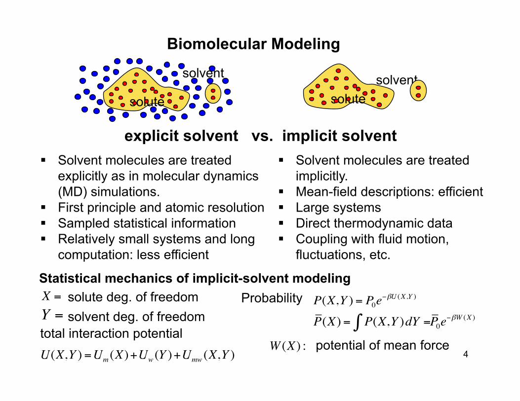
Biomolecular Modeling
explicit solvent vs. implicit solvent § Solvent molecules are treated
explicitly as in molecular dynamics (MD) simulations.
§ First principle and atomic resolution § Sampled statistical information § Relatively small systems and long
computation: less efficient
§ Solvent molecules are treated implicitly.
§ Mean-field descriptions: efficient § Large systems § Direct thermodynamic data § Coupling with fluid motion,
fluctuations, etc.
Statistical mechanics of implicit-solvent modeling X =Y =
solute deg. of freedom solvent deg. of freedom
total interaction potential U(X,Y ) =Um (X)+Uw (Y )+Umw (X,Y )
Probability P(X,Y ) = P0e−βU (X,Y )
P(X) = P(X,Y )dY =∫ P0e−βW (X )
potential of mean force W (X) :4
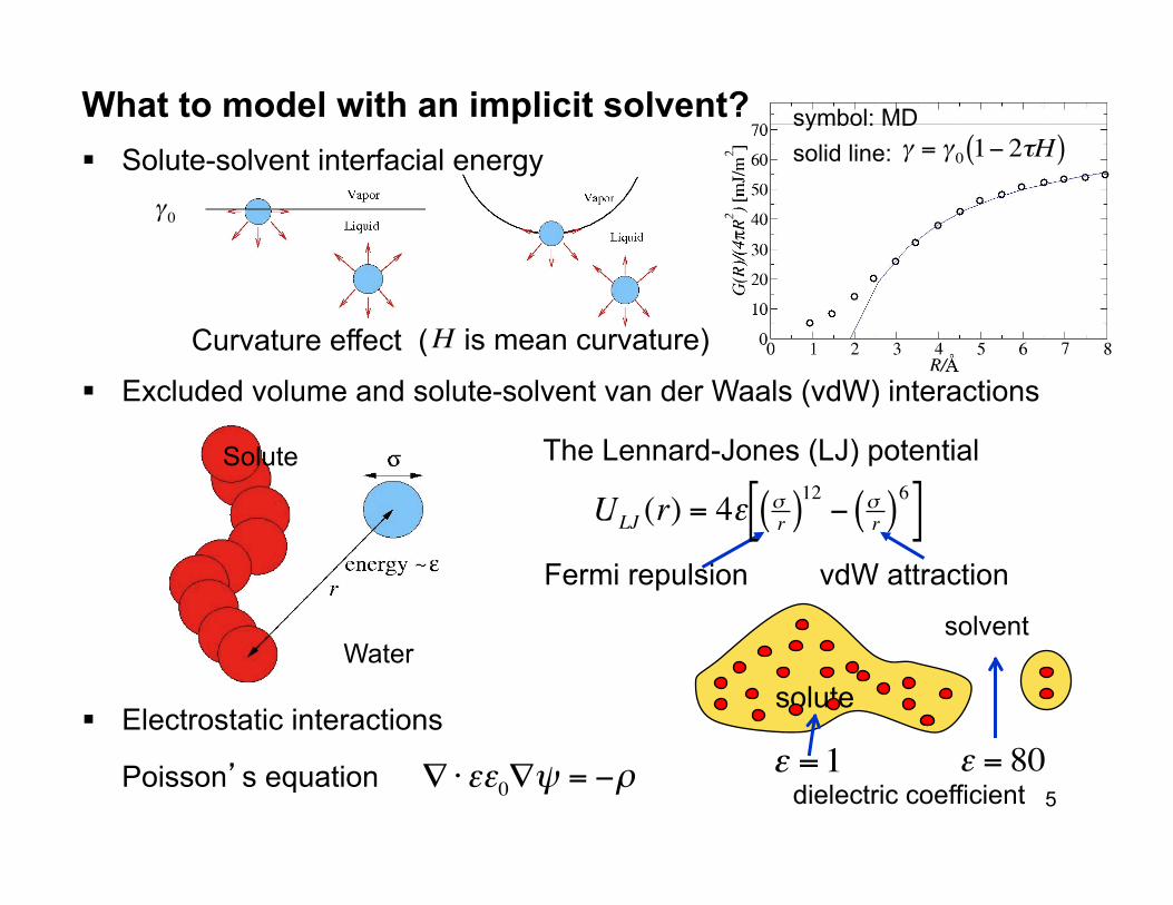
§ Solute-solvent interfacial energy
€
γ = γ 0 1− 2τH( )
Curvature effect (
What to model with an implicit solvent?
§ Electrostatic interactions
€
∇ ⋅εε0∇ψ = −ρPoisson’s equation
solvent
solute
€
ε =1
€
ε = 80
Fermi repulsion vdW attraction
Solute
Water
§ Excluded volume and solute-solvent van der Waals (vdW) interactions
€
ULJ (r) = 4ε σr( )12 − σ
r( )6[ ] The Lennard-Jones (LJ) potential
is mean curvature) H
symbol: MD solid line:
€
γ 0
dielectric coefficient 5
Surface energy
PB/GB calcula1ons
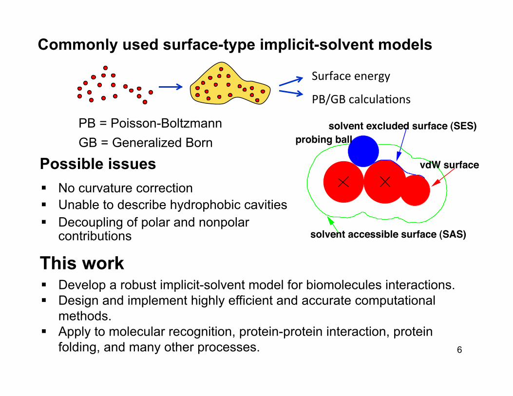
Commonly used surface-type implicit-solvent models
solvent accessible surface (SAS)
probing ball
vdW surface
solvent excluded surface (SES)
Possible issues § No curvature correction § Unable to describe hydrophobic cavities § Decoupling of polar and nonpolar
contributions
PB = Poisson-Boltzmann GB = Generalized Born
This work § Develop a robust implicit-solvent model for biomolecules interactions. § Design and implement highly efficient and accurate computational
methods. § Apply to molecular recognition, protein-protein interaction, protein
folding, and many other processes. 6

Koishi et al., PRL, 2004. Liu et al., Nature, 2005. Sotomayor et al., Biophys. J. 2007
7
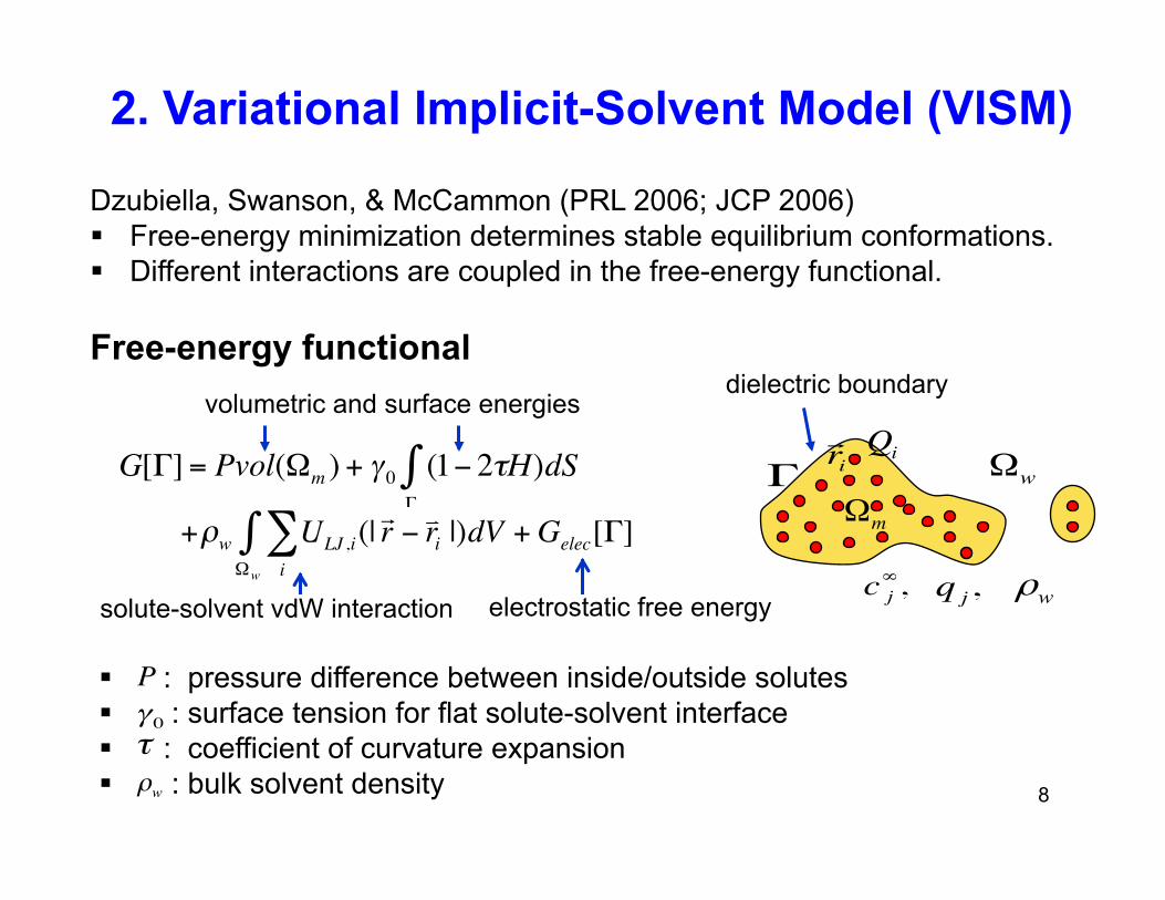
§ : pressure difference between inside/outside solutes § : surface tension for flat solute-solvent interface § : coefficient of curvature expansion § : bulk solvent density
Free-energy functional
€
r i
€
Ωm
Γ
€
Qi
€
Ωw
€
c j∞,
€
q j , wρ
€
G[Γ] = Pvol(Ωm ) + γ 0 (1− 2τH)dSΓ
∫
€
+ρw ULJ ,ii∑
Ωw
∫ (| r − r i |)dV + Gelec[Γ]
ρw
2. Variational Implicit-Solvent Model (VISM)
dielectric boundary volumetric and surface energies
solute-solvent vdW interaction electrostatic free energy
P
τγ0
Dzubiella, Swanson, & McCammon (PRL 2006; JCP 2006) § Free-energy minimization determines stable equilibrium conformations. § Different interactions are coupled in the free-energy functional.
8
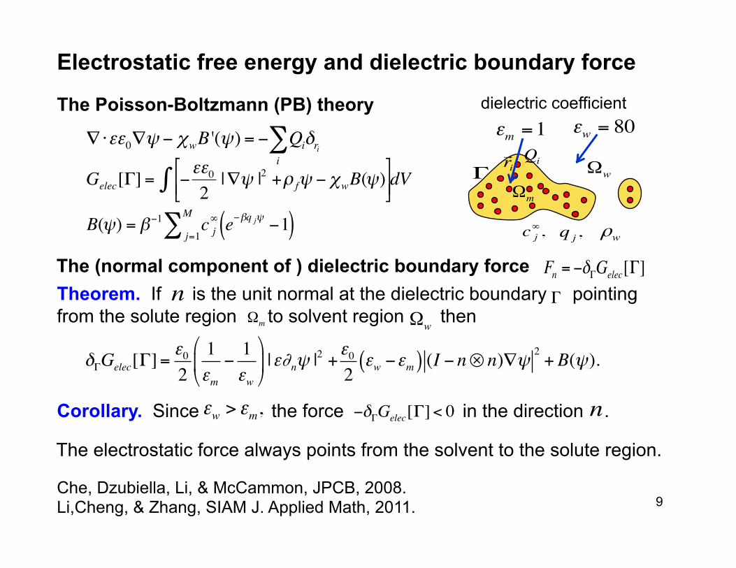
Electrostatic free energy and dielectric boundary force
The Poisson-Boltzmann (PB) theory
∇⋅εε0∇ψ − χwB '(ψ) = − Qiδrii∑
€
B(ψ) = β−1 c j∞ e−βq jψ −1( )j=1
M∑
€
r i
€
Ωm
Γ
€
Qi
€
Ωw
€
c j∞,
€
q j , wρ€
εm =1
€
εw = 80
€
Gelec[Γ] = −εε02|∇ψ |2 +ρ fψ − χwB(ψ)
)
* + ,
- . ∫ dV
dielectric coefficient
The (normal component of ) dielectric boundary force Fn = −δΓGelec[Γ]Theorem. If is the unit normal at the dielectric boundary pointing from the solute region to solvent region then
δΓGelec[Γ]=ε02
1εm
−1εw
#
$%
&
'( |ε∂nψ |
2 +ε02εw −εm( ) (I − n⊗ n)∇ψ 2
+B(ψ).
nΩm Ωw
Corollary. Since the force in the direction . εw > εm,
Γ
The electrostatic force always points from the solvent to the solute region.
−δΓGelec[Γ]< 0 n
9 Che, Dzubiella, Li, & McCammon, JPCB, 2008. Li,Cheng, & Zhang, SIAM J. Applied Math, 2011.
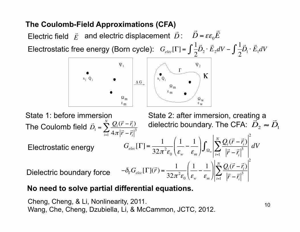
The Coulomb-Field Approximations (CFA)
€
D 2 ≈
D 1
€
Gelec[Γ] =12∫ D 2 ⋅ E 2dV −
12∫ D 1 ⋅ E 1dV
Electric field and electric displacement : E
D = εε0
E
No need to solve partial differential equations.
!xi
!"
"
#"#
iQi
#
"
Qx iG$
wwm
m
m
m
%
& &
Electrostatic free energy (Born cycle):
−δΓGelec[Γ](r ) = 1
32π 2ε0
1εw−1εm
#
$%
&
'(
Qi (r − ri )r − ri
3i=1
N
∑2
Gelec[Γ]=1
32π 2ε0
1εw−1εm
#
$%
&
'(
Qi (r − ri )r − ri
3i=1
N
∑Ωw∫
2
dV
D1 =
Qi (r − ri )
4π r − ri3
i=1
N
∑The Coulomb field
D
State 1: before immersion State 2: after immersion, creating a dielectric boundary. The CFA:
Electrostatic energy
Dielectric boundary force
10 Cheng, Cheng, & Li, Nonlinearity, 2011. Wang, Che, Cheng, Dzubiella, Li, & McCammon, JCTC, 2012.

Coupling solute molecular mechanics with VISM
€
V[ r 1,..., r N ] = Wbond
i, j∑ ( r i,
r j ) + Wbendi, j ,k∑ ( r i,
r j , r k )
€
+ WCoulombi, j∑ ( r i,Qi;
r j ,Qj )
€
H[Γ; r 1,..., r N ] = V[ r 1,...,
r N ]+ G[Γ; r 1,..., r N ]
€
minH[Γ; r 1,..., r N ] equilibrium conformations
An effective total Hamiltonian
+ WLJi, j∑ (ri,
rj )
Force field of solute mechanical interactions
+ Wtorsion (ri
i, j,k,l∑ , rj,
rk,rl )
11
Cheng, Xie, Dzubiella, McCammon, Che, & Li, JCTC, 2009.

€
Vn = Vn ( r ,t)
€
r ∈ Γ(t)§ Level-set representation
€
Γ(t) = { r ∈ Ω :ϕ( r ,t) = 0}§ The level-set equation
)(tΓ
n
€
r § Interface motion by the normal velocity
for
0|| =∇+ ϕϕ nt V)(tΓ
€
z =ϕ( r ,t)
0=z
3. The Level-Set Method
§ Easy handle of topological changes
§ Level-set formulas of geometrical quantities Unit normal Mean curvature Gaussian curvature Surface integral Volume integral
H =∇⋅n / 2
n =∇ϕ / |∇ϕ |
€
K = n ⋅ adj(He(ϕ)) n
€
f ( r )dS =Γ∫ f ( r )δ(ϕ)dV
R 3∫
€
f ( r )dV =Ω∫ f ( r )[1−H(ϕ)]dV
R 3∫ 12
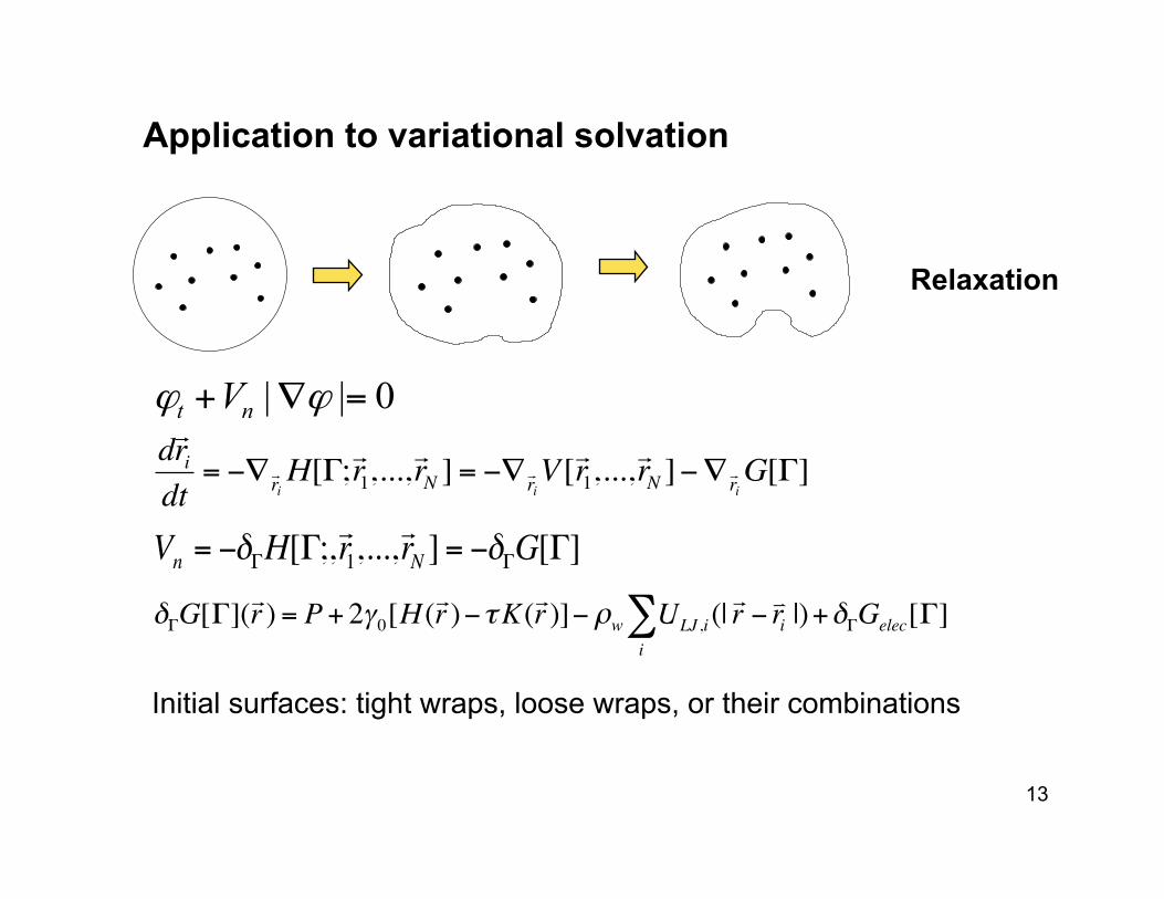
Application to variational solvation
δΓG[Γ](r ) = P + 2γ0[H (
r )−τK(r )]− ρw ULJ ,ii∑ (| r − ri |)+δΓGelec[Γ]
Relaxation
€
Vn = −δΓH[Γ;, r 1,..., r N ] = −δΓG[Γ]
€
d r idt
= −∇ r iH[Γ; r 1,...,
r N ] = −∇ r iV[ r 1,...,
r N ]−∇ r iG[Γ]
0|| =∇+ ϕϕ nt V
Initial surfaces: tight wraps, loose wraps, or their combinations
13
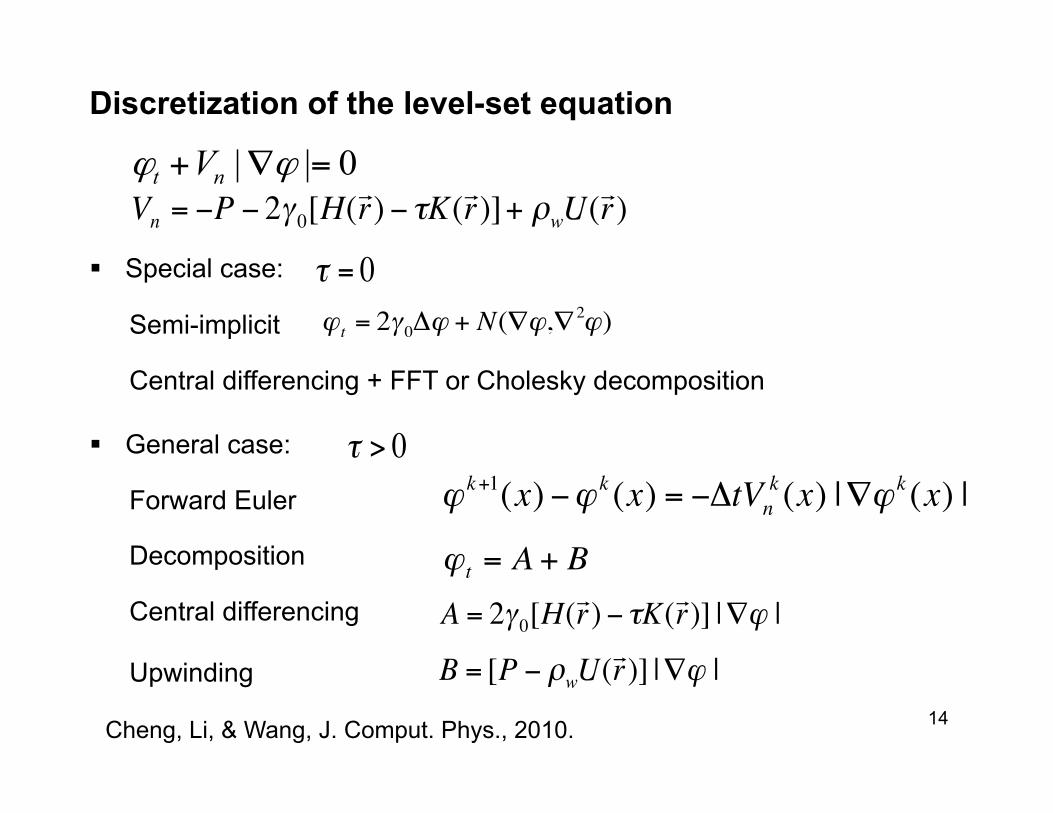
Discretization of the level-set equation
0|| =∇+ ϕϕ nt V
€
Vn = −P − 2γ 0[H( r ) − τK( r )]+ ρwU( r )
€
ϕ k+1(x) −ϕ k (x) = −ΔtVnk (x) |∇ϕ k (x) |Forward Euler
Decomposition
€
ϕ t = A + B
€
B = [P − ρwU( r )] |∇ϕ |
€
A = 2γ 0[H( r ) − τK( r )] |∇ϕ |Central differencing
Upwinding
€
τ = 0
€
τ > 0
Central differencing + FFT or Cholesky decomposition
Semi-implicit
§ Special case:
§ General case: €
ϕ t = 2γ 0Δϕ + N(∇ϕ,∇2ϕ)
14 Cheng, Li, & Wang, J. Comput. Phys., 2010.

Potential of mean forces (PMF): Level-set (circles) vs. MD (solid line).
2 3 4 5 6 7 8 9 10 11 12d/
-2
-1
0
1
2
w(d
)/k
BT
3 4 5 6 7 8 9 10 11
-1
0
1
W(d
)/k
BT
Å
two xenon atoms two paraffin plates
4. Test and Applications
15 Cheng, Dzubiella, McCammon, & Li, JCP, 2007.

Helical alkanes and C60 fullerene
16
17
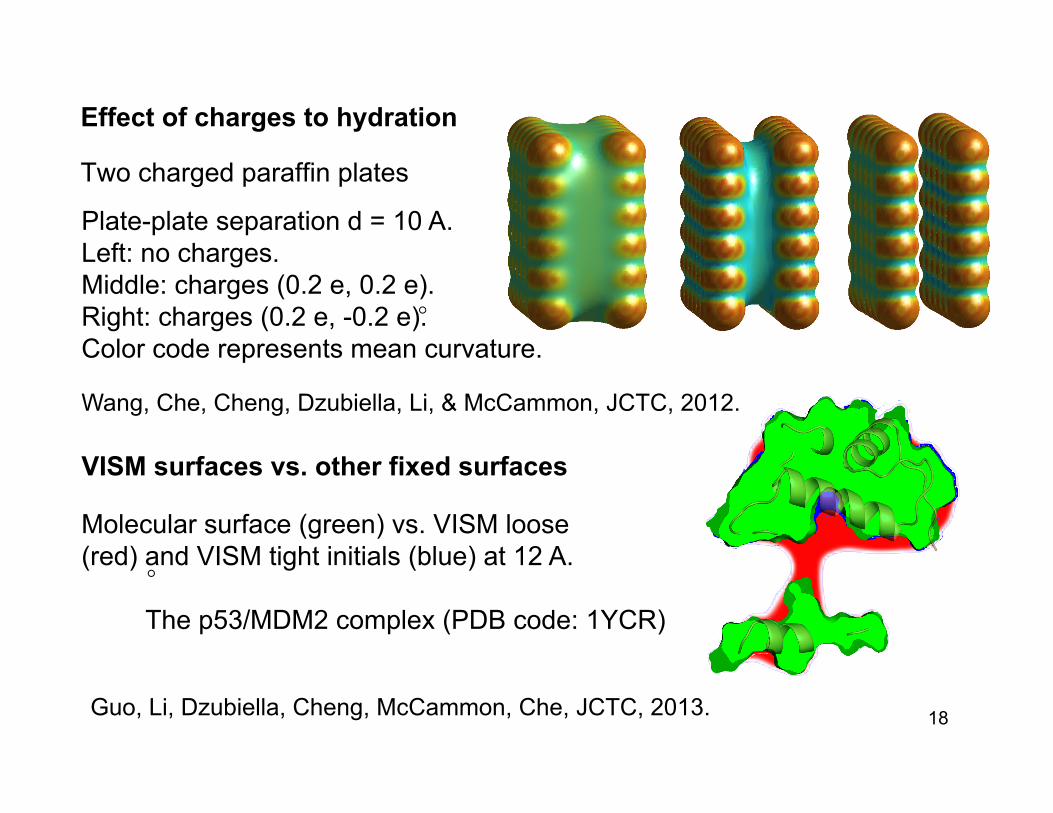
Two charged paraffin plates
Plate-plate separation d = 10 A. Left: no charges. Middle: charges (0.2 e, 0.2 e). Right: charges (0.2 e, -0.2 e). Color code represents mean curvature.
Effect of charges to hydration
VISM surfaces vs. other fixed surfaces
The p53/MDM2 complex (PDB code: 1YCR)
Molecular surface (green) vs. VISM loose (red) and VISM tight initials (blue) at 12 A.
18
Wang, Che, Cheng, Dzubiella, Li, & McCammon, JCTC, 2012.
Guo, Li, Dzubiella, Cheng, McCammon, Che, JCTC, 2013.
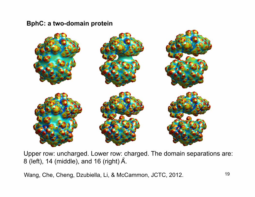
BphC: a two-domain protein
Upper row: uncharged. Lower row: charged. The domain separations are: 8 (left), 14 (middle), and 16 (right) A.
19 Wang, Che, Cheng, Dzubiella, Li, & McCammon, JCTC, 2012.

20
!! !" # " ! $ % &#"#!
"#$
"#%
"&#
"&"
"&!
"&$
'()*+,
-./010.(
'()*+,23/240+5(627./010.(
0(010542.8219.2/:5442)(3)4.7)0(010542.82.()245*+)2)(3)4.7)
PMF
particle-wall distance
A receptor-ligand system p53/MDM2
uncharged charged
A host-guest system CB[7]-B2
Cheng, Wang, Setny,Dzubiella, Li, & McCammon, JCP, 2009. Setny, Wang, Cheng, Li, McCammon, & Dzubiella, PRL, 2009. Zhou, Rogers, de Oliveira, Baron, Cheng, Dzubiella, Li, & McCammon, 2013.
21

22

" Coupling solute molecular mechanics " Effective dielectric boundary force " The Coulomb-field approximation of electrostatic energy
" Estimates of solvation free energy " Hydrophobic cavities and multiple states of hydration " Charge effect
Summary
€
G[Γ] = Pvol(Ωm ) + γ 0 (1− 2τH)dSΓ
∫
€
+ρw ULJ ,ii∑
Ωw
∫ (| r − r i |)dV + Gelec[Γ]
VISM free-energy functional
The level-set method: algorithm and coding
Numerical computations
5. Conclusions
23
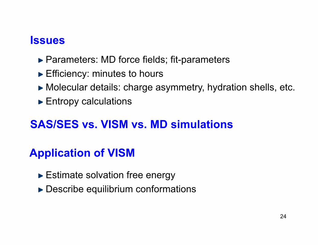
" Parameters: MD force fields; fit-parameters " Efficiency: minutes to hours " Molecular details: charge asymmetry, hydration shells, etc. " Entropy calculations
Issues
SAS/SES vs. VISM vs. MD simulations
Application of VISM " Estimate solvation free energy " Describe equilibrium conformations
24
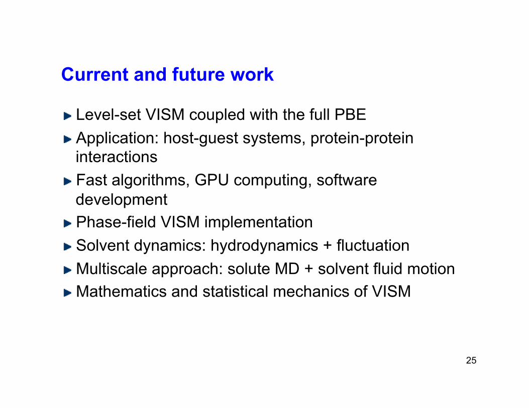
" Level-set VISM coupled with the full PBE " Application: host-guest systems, protein-protein
interactions " Fast algorithms, GPU computing, software
development " Phase-field VISM implementation " Solvent dynamics: hydrodynamics + fluctuation " Multiscale approach: solute MD + solvent fluid motion " Mathematics and statistical mechanics of VISM
Current and future work
25
Funding: NSF, DOE, NIH, CTBP
Joachim Dzubiella (Humboldt Univ.) J. Andrew McCammon (UCSD) Li-Tien Cheng (UCSD) Jianwei Che (GNF) Zhongming Wang (Florida Intern’l Univ.) Piotr Setny (Munich & Warsaw) Zuojun Guo (GNF)
Main Collaborators
Acknowledgment
26

Thank you!
27
References
[1] Dzubiella, Swanson, McCammon, PRL, 96, 087802, 2006. [2] Dzubiella, Swanson, McCammon, JCP, 124, 084905, 2006. [3] Cheng, Dzubiella, McCammon, & Li, JCP, 127, 084503, 2007. [4] Che, Dzubiella, Li, and McCammon, JPC-B, 112, 2008. [5] Cheng, Xie, Dzubiella, McCammon, Che, & Li, JCTC, 5, 257, 2009. [6] Cheng, Wang, Setny, Dzubiella, Li, & McCammon, JPC, 113, 144102, 2009. [7] Setny, Wang, Cheng, Li, McCammon, & Dzubliella, PRL, 103, 187801, 2009. [8] Cheng, Li, & Wang, J. Comput. Phys., 229, 8497, 2010. [9] Cheng, Cheng, & Li, Nonlinearity, 24, 3215, 2011. [10] Li, Cheng, & Zhang, SIAM J. Applied Math, 71, 2093, 2011. [11] Wang, Che, Cheng, Dzubiella, Li, & McCammon, JCTC, 8, 386, 2012. [12] Cheng, Li, White, & Zhou, SIAM J. Applied Math, 73, 594, 2013. [13] Guo, Li, Dzubiella, Cheng, McCammon, & Che, JCTC, 9, 1778, 2013. [14] Zhao, Kwan, Che, Li, & McCammon, JCP, 2013 (accepted). [15] Zhou, Rogers, Oliveira, Baron, Cheng, Dzubiella, Li, & McCammon, JCTC,
2013 (submitted)
28
Top Related