


Languages
Pages
Legal


..
. , ,
,
VARIABLE lENGTH COOING FOR CORREL-ATE[)Io I~RMATION SOURCES
\
, '\
-- David W. Boiley, B.Eng ..
A thesis subrnifted to the Faculty of Graduate Studies ond Reseorch .
in partial fulfi"me'nt of the requirements for the degree of
Master of Engineering.
" Department of Electrical Engineering,
•• '<'
;
\
~cGill University,
fV'\ontreal, Quebec •
Morch, 1975.
David W. Bailey 1975 ",
...
J

/' /
. ., ABSTRACT
The theory of variable length coding for a discrete memoryless in- ,
( -formation source is extended to the problem of two.correlated sources. It is weil
known that the output sequence from a single source X con be encoded and
subsequently reconstructed by a decoder with zero probability of error if and only 1
if the average codeword length n satisfies n ~ H (X). This familiar conclu-x x
.,.. sion is generalized to cover correlated source éoding un~er several q.ifferent
assllmptions about the enc:oders and decoders. A method is deve loped to determine ,i
what minimum average codeword lengths n and n are needed in order to achieve x y
zero-error communication for any pair of .. correlated sources X and Y. The results \
are presented as an admissible rate ~region in the n - n plane. x y
f' .
~ "
,',
1·
!

. >
.. • ~, ... 1 .. \ ........ i i
RESUME
la th:orie du codagè à longueur variable pour une .. source d'informa-.' .~
tion discrète sanS mé'moire est ~tendue au cas de deux sources corre lI~es: "est
bien connu que la s6qûence de sortie d'lune source unique X peut être codée et J
par la suite reconstruite par un d~codeur avec une probabilité nulle d'erreur si et
" seulement si la longueur moyenne n du mot cod~ satisfait la relation ri ~ H (X) x . X
r
Ce fait connu est g~né'ralisé au cas de codage de sources correllées, grâce ~ un
~ l certain nombre d'hypothhe's concernant les codeurs - décodeurs. Une mé'thode,
, permettant de dé'termlner les longueurs moyennes ~inimales n et n des mots x y
cod~ afin d'obtenir la communication sans erreur pour deux sou.rces correllées X
'" l '" et y, est deve oppee. Les~résultats sont présent~s sous forme d'une région ~ taux
admissibIe dans le plelO n - n (~ y /
, ..
J
.' "
",' .. , \,
'"

, "
-, "
.;
"
ACKNOWLEDGEMENT , : (
, '
The a~thor expresses sincere thanks to Dr. Michael J. Ferguson
<il
who proposed and supervised the project. His patience and encouragement
were greatly appreciated.
1
~ M.s. Hyland did an exce lient job of typing. The author thanks
her.
This re~earch was 'supported by tlie National Research Council
of Canada. '.
,1
'~
iii
:'

1
".
<.>
AB5TRACT
RESUME
, . /1
TÂBLE OF (CONTENTS
, , )
ACKNOWlEDGEMENT r
TABLE Of CONTENTS 1
(,
CHAPTçR
CHAPTER
CHAPTER
CHAPTER
CHAPTER
CHAPTER
/ !
REFERENCES
1
INTRODUCTION t
(1
If VARIABLE LENGTH CODING"
III
IV
v
VI
"--- F OR A 51 NGLE SOURCE \
,~_/' f Q
~DING F<2R CORR.ELATED $OORCES
/l'AN ALGORIT~~ FOR DET,ERMINING
\ THE ADMISSIBLE REGION
ALTERNATIVE - CONFIGURAT IONS /IN CORRELATED SOURCE CODING
. CONCLU SION
" t
iv ,
ii
i i i ,
iv'
• ~ r
J 8 , 0 . . :
i' 14
42
71
90
95

1 \
CHAPTER 1
INTRODUCTION 1"
The purpose of this thesis is to extend the f?mi 1 iar the ory of variable
length coding for a discrete meinoryless information source to the more general
situation of two corre \ated sources.
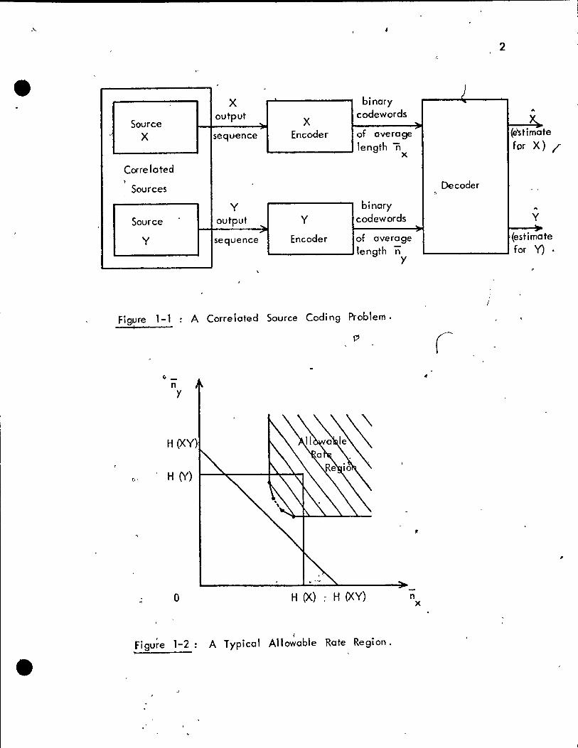
One of the most interesting problems concerning correlated source
. ~
coding results when the encoders a~ decoders are arranged as illustrate~ in Figure
1-1. Notice that al1hough, each encoder is restricted to see the output sequence
t Irom only one sourc~, the decoder js ollowed to observe both of the encoded messoge
\treams. Systems of this type (and o~her re lated configurations) are studied in
detail in this thesis to determine what minimum average codeword lengths n and n x y
are required by the encoders in order that the· decoder con reconstruct the source
output sequences with zero probability of error. The results are presented as on
allowable rate region in the n - n plqne. x y,
As will be shown in Chapter III, a typical problem having the form
of Figure 1-1, might have an allowqble rate region of the nature indicated in Figure
1-2. The important implication of such a rate region is that it is possible for the out-'
puts of two correlated sources to be communicated-to a decoder with zero distortion
by using encoders whose average codeword lengths satisfy ÎÏ < H (X) and " x
~ < H (Y). This is an improvement over the classital situation illustrated in y
Figure 1-3, in which the two sources are encoded and decoded independently, which
Source X
Correlated l
Sources
Source
y
FigJJre 1-1 1
~-n y
o
Figure 1-2
, -X binary
output codewords ... X ...
sequence Encoder of average length "il
x
y binary
output .... Y codewords ...
Encoder sequence of average length -n
y
A Correlated Source Coding Problem.
H (X) ~ H (XY)
A Typical Allo~able Rate Region.
ft
n x
2
) ,.
,. X.
(e'stima te for X )/
Decoder . , 0
" y
~ .... estima te for Y)
,

SE
(\ \
. ,
- ,. n
Source X X , X X_ x
X Encoder " Decoder
Correlated " Sources
-y
n y~ Source , y y y
y Encoder ~
Decoder
.1
Figure 1-3: Independent Coding for Correlated Sources.
..
, ~ "

..
4
requires that n ~ H (X) ând n ~ H (Y). Therefore, there is a special interest 'x ~
in studying the problem of coding for correlated sources, the goal being to discover
how to take advantage of this correlation between source output sequ~nces in de-
sigtjling the best possible enc?ders and decoders. 5ince the well-known Huffman ()
code is the procedure for constructing optimum codes for a single information source,
the main theme of this thesis con be summarized as being the generalization of the
Huffman code to the case of two correlated sources
The correlated source coding problem illustrated in Figure 1-1 is only 1
one of several related systems to be considered in this thesis. As indicated in
1
Figure 1-4, there exist sixteen different arrangements for the encoders and decoders
corresponding to 011 possible ways of positioning the fo"switches 51' 52' 53' a'1d
S4' Notice that the configurati on of Figure 1-1 is just\he situation which occurs
when switches 51 and 52 are open with 53 and 54 cl osed.
Th~ subject of t~is thesis, as introduced above, is one of several in"\
teresting topies eoneerning the joint coding of eorrelated sources. Although most of
these problems still remain unsolved, two important contributions in this area have
recently been reported in the literature. Siepian and Wolf 'L4J considered the pro-
blem of fixed length or block coding for correlated sources. For 011 of the configura-
tions of Figure 1-4, they determined what minimum numbers of bits per character were
needed in order to communieate the source output sequences to the decoder with
arbitrari Iy sma \1 decoding error probobi lities. Of course, this dîffers From the problem
.. 1

"
5 (ft
r
/
x h ,.
Source , X x ... X K. ,.
X Encoder Decoder
41\ II' --Correlated
Sl 53 , Sources - -
." ~ --~
'S 54 < 2
~ , \i'
Sovrce - y ,.
y y n y
... y . -y ~ Encoder ., Decoder ,.
~ / .... (
Figure 1-4: Sixteen Correlated Source Coding Configurations.
"
. "
•

of variable length coding which employs a ~ probability of error criterion. A
paper published by Wyner [5J established a similar result, again con~erning fixed o
6
length coding for joint,sources. The author of this thes.is believes thàt the problem
of variable length coding for correlated information sources has until this time been .. unsolved and that consequently the solutions which are presented in this thesis are
contributions to original knowledge.
The material studied in this thesis is orgonized in the following manner.
Çhapter Il contains a brief review of various fundamental results on variable length
coding for a single source. Some useful quantitie! su ch as entropy and average code-
word length are defined, followed by a statement of three well-known source coding
theorems ~
ChaRter III is devQted to studying the correlated source coding s~tem of
Figure 1-1. First of 011, the problem is defined pr1cisely and then a theory is
developed _starting From first principles. Several examples of varying diHiculty are
presented to aid in illu~ating many of the new ideas.
ln Chapter IV, the results of Chapter III are exploited in devising a
practical method for solving the problem of Figure 1-1 for any given pair of corre lated
sources.
program . ,.,
.. The form of this algorithm allo~o be impie
.-A report is given -on how efficiently su ch e p
lJsed to solve specifie exemples.
nted easilYlby a computer
\ 9 al11 performetl when it wes
. )
. ....

(
-t,
The purpose of-(:hapter V is to extend the results of Chapters III and Cl
IV 1 valid only for the system of Figure 1-1, to the other fifteen cdding configura-"
tion~ of Figure 1-4. Fortunately, it turns out that onl? ~inor modi'fication,s to the
methods of Chapter IV a,re nece~sary. Fina Ily 1 Chapter VI is a summary of sorne
. /"
of the more important results of thi"s fhesis, together with a mention of sorne related v
topics whkh might be areas of future research .
. -,.)
.' , -
f, ,) \,
t y • .'
,
E> .4 , [<~
'. ~f , 4"
,
"
'.

! , .- 1
" CHAPTER Il
VARIABLE LENGTH CODING FOR A SINGLE SOURCE
The the ory of variable length coding for a single information souJce cJ t.
is weil knownjs/e~; Gallager [2, pp. 43-55J). This chapter is devoted to~re-
8
r 1 - " '-
viewing some 'of the important results of ,this theory, results which will subsequently l'
be QPplied when solving the problem of coding for correlated sources.
1
Therefore, consid'er the classical source coding problem i Ilustrated in
Figure 2-1. Here, source X is assumed to be a discrefe memoryless source:. This
means that each unit of time, the source produces one of a finite set of source letters,
say xl' x2' ... , xk
' with a fixed set of probobi lities Pr (xl)' Pr (x2)' ... , and
Of course, these probobil ities must satisfy "
k \"' L Pr (x.) = 1 .
• ' 1
i=l
, .-C'--T,he information rate of source X is described bya very important quantity calle, the
entropy of source X • It is defined by <
k
~ - L Pr (Xi) 1092 Pr (Xi) ,
, i=l
" ,
vihere H (X) Îs the entropy expressed in units called bits of information.
". '''; --
t."-o_

e ••
.f
.,f,
. .
.',
...
Source X
X output '",
~ sequence,
. "
... ..
"
"
.J
binary Source codewords
Encoder of averagê
length 1'\"
Figure 2-1 The single source cocling problem.
..
9
,
- e--
Decoder ... ~ • "7 estlm ~
ate for X )
;u <-('

The function of the source encoder is to represent each source lefter
~
by a codeword consisting of a sequence of binary letters. More precisely, the en-
coder performs a one-to:'!.ne mapping from the k source letters xl' x2
' ... , xk
'
to a set of k binary codewords having lengths ml' m2
, ... , a,nd mk
. The
average todeword length ïi turns out to be a very useful measure of performance and
is defined by
" k ) Il. c-.
"il == \ m. Pr (x.) . Lr 1 1
i= 1
The decoder for the system of Figure 2-lt,~ performs the following
operations. It observes the sequence of binary letters coming from the source en-
coder and -based on this information produces X, an estimate of the original source
, output X. It is desirable to design the source encoder in such a way that the de-
codèr can reconstruct the source output sequence with zero probability of error. In
order for thE requirement to be met, it is necessar~ and sufficient to choose the set of
k codewords to be unique Iy decodable. This means that any finite sequence of
binar<, symbols from the source encoder can be uniquely resolved into sequences of
codewords. Il
The obiective in studying the system of Figure 2-1, is to determine how
to design the best possible source encoder. The optimum encoder is defined to be the
one which has the minimum possible average codeword length n with the restriction

11
that the code must be uniquely decodable. The following familiar theorem sheds
sorne light on the subject of optimum encoders.
t l \
T~eorem 2-1: ((or proof, see [2, pp. 50-51]) ~' ,
~or the system illustroted in Figure 2-1, it is possible to Qssign codewords to the
source letters su ch that the code is uhique Iy decodable and such t~at the average
codeword length ri satisfies
Il
n < H (X) + 1 .
Il
Furthermore, for any unique Iy decodable code of this type, it is necessary that
n ~ H (X) .
Although Theorem 2-1 does not in te exactly how to design an
optimum source encoder, it does establish t """----.I_~, timum system has an average
codeword length somewhere in the range
H (X) ~ n < H (X) + 1 !
A stronger theorem con be establi hed y allowing the source encoder
to assign codewords t,o sequences of L source le -.....
" \
Specifically, the encoder
can be redefined as being a one-to-one mapping from the set of kL different source
sequences of len.gth L to a uniquely decodable set of kl binary ~odewords. For
this more general situation, the following theorem can be shown to apply.
... \

12
Theorem 2-2: (for proof 1 see [2, p. 51 J)
For the system showQ in Figure 2-~ 1 it is possible to assign codewords to $equences
of l source letters such that the code is unique Iy decodable and such that the average
codeword length 'fi satisfies
n < H (X) + 1 Il .
" - '" Furthermore, for any uniquely decodable cod~ of this generalized type, it tS
necessary that
n ~ H (X) .
This theorem establishes that in general, the optimum source encoder I-I
has an average codeword length n somewher~}n the range r, 1
" H (X) ~ n < H (X) + l 1 l . ;-
~ ;'
The actual finding of this optimum code can/be accomplished by opplying a fomeçJ 1 . ,
constructive procedure called the HuHmon ~ode' (see Gal/,ager [2,' pp. 52-55) . .!. • ,
.'
The key consequence of Theorem 2-2 is that by mal<ing L arbitrarily la~ge (that -
1
is, by assigning codewords to orbitrarily ,fong sourqe sequences), it is possible to "
design a source encoder with an averafe codeword le,?gth n ~hich is arbitrarily , ,
close to H (X). This result is ~.~eirized by the fo.llowing theorem. ~... ","
!,~ ...
Pi

13
Theorem 2- 3 : The output sequence from source X for the .system .'
of Figure 2-1, con be communicoted to the decoder with zero probobility of error
if and only if the average codeword length for the source encoder sotisfies
-n ~ H (X) •
/
i.: ..
l'
.~""I
/
.'
/ /

; (
'.
CHAPTER III
COOl NG FOR CORRElATED SOURCES
The theory of variable length codjng for a single information source
(as reviewed in Chapter Il) will now be generalized to the correlated source cod-
, "" ing problem illu~l*ated in Figure 3-1.. This is the sorne problem which was
:i-,~
initially intrOduced in Chapter 1 (see Figure l-}).
ln the following discussions, it Wtll be assumed that both source X
and source Y ore discrete memoryless sources. This irnP1fes that during each 1
unit of time, source X produces one of a finite set of source letters, say
Xl' x2
' ..• , xk
' and simultaneously source Y produces one letter From the set
J y 1 ' Y 2' ..• , y q' Successive occurrences of (X, y) pa i rs are i ndep;fdent and
are governed by' the fixed set çf probabil ities
( Pr (x. , y.) 1 1
i = l, 2, ... , k i = l, 2, .•• , q } ,
11 where of course
k q
I L (,
Pr (x. , y. ) . '
= -, 1 1
i=l j=l
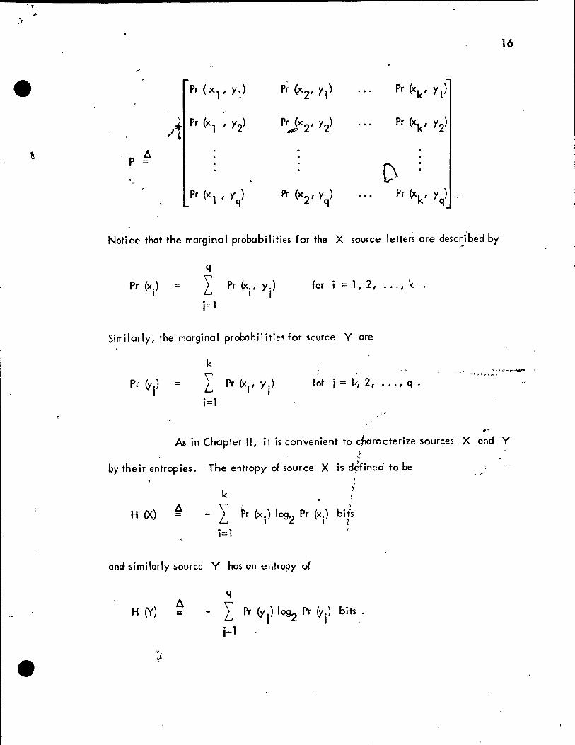
, The correlation between sources X and y is best summarized by arrangihg the
given set of probabitities into a q x k probobility motrix P as follows :
v

15
,
" ,
~ / tl'
~
: (
-X
n ,z Source X
x -~ ...
X Encoder ~
Correlated Decoder
Sources
1 -Y
n ~ Source
~ y y ... -, -.,- ~
y Encoder
-
Figure 3-1 A correlated source coding probl~m. '~"
. , ·>
"
Notice that the marginal probabilities for the X source letter~ are desc~fbed by
Pr (x.) 1
= q
l j=l
for =1,2, ... ,k . Pr (x., y.) 1 1
Similarly 1 the marginal probabi 1 ities for source Y are
Pr (y.) 1
=
k
l i=l
(
Pr (x., y.) 1 1
for i = 1.:, 2, ... , q .
"
16
As in Chapter Il, it is convenient to c~aracterize sources X and Y y' "
by the ir entropies. The entropy of source X is d~fined to be '1
k
H (X) ~ '\ Pr (x.) 1092 Pr (x.) bds L III i=l ~
and, similarly source Y has an el,tropy of
H (Y)
" If:
A ::
q
l Pr (y i) 1 092 Pr (y j ) bits .
j;;: 1
) However, this is only a partial characteri~otion becouse there is a dependence
between the two sources. For this reason, it is necessary to introduce H (XY)
the joint entropy of sources X and Y. This importont~ntity is defined by
k A r
H (XY) = - l q
L i=l j=l
Pr (X., y.) 1092 Pr (X., y.) bits . 1 1 1 1
17
These entropies wilJ appeor often in subsequent derivations regarding the correlated
source coding problem.
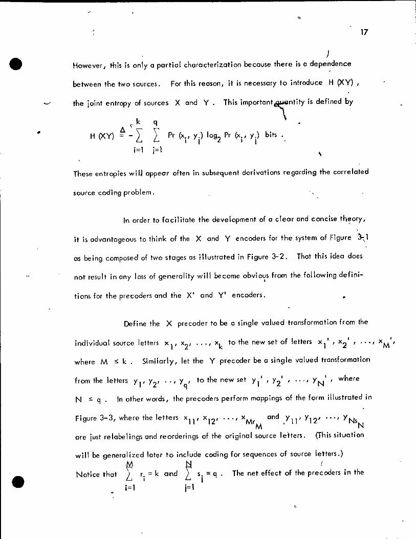
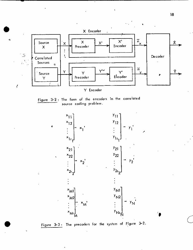
ln order to fa ci litote the development of a c1eor and concise th~ory, ,
it is advontageous to think of the X and Y encoders for the system of Figure ~ 1
as being composed of two stages as illustrated in Figure 3-2. Thot this idea does
not result in any loss of generality will become obvious from the following defini-,
tions for the precoders and the XI and Y' encoders. •
Define the X precoder to be a single valued transformation from the
individual source letters xl' x2
' ... , xk
to the new set of letters xli, x21
, ••• , xMl,
where M ~ k. Similarly, let the Y precoder be a single valued transformation
fromthe letters Yl' Y2' .. , Yq' tothenewset Y11
, Y2', ... , y N ', where
N ~ q. In other words, the precoders perform mappings of the form illustrated in
Figure 3-3, where the letters x ll ' x 12 ' .•. , xMrM
and /11' Y12' ..• , YNsN
are just relabelings and reorderings of the original source letters. (This situation
will be generalized later to include coding for sequences of source letters.)
Notice thot f ri = k and ~ Si = q The net effect al the precoders in the
i= 1 j= 1
l,
-18
X Encoder >
-Source X XI
X XI n ~ X Preceder
.. Encoder x , ,
) • -
.. Corre loted 1 .. Decoder
Sources 0
-- Source
y yltl n 'Y ~ y yi Y
Y Precoder ... jo .. ~ ..
Encoder
" : (
Y Encoder
figure 3-2 : The form of the encoders in the corre loted
source coding problem.
x l1 Yll
x l2 YI2
" Xl Y 11 .... .... 1
xl r YIs 1
x2I Y21
x22 Y22
.... x 1 .... Y2
1
2
x2r Y2s " 2
x'Ml YNl
xM2 YN2
.... 1 .... 1
xM YN
x YNs MrM
:, c Figure 3-3: The precoders for the system of F}gure 3-2.

e.
19
system of Figure 3-2 is to transform sources * and vY into simpler sources X'
and yi. These new sources con be describe'cl by entropies H (X') and H (Y')
respectively where H (X') is defined by
M' H (X')
A L Pr (x. ') 1092 Pr (X. ') - 1 . 1
". i=l r. r.
M ." 1 1 1 4-
-I --, \'
= [ L Pr (x .. ) J 1092
[ L Pr (x •. ) ] bits , Il IJ
i= 1 j=l j=l
and H (YI) is defined in a similor fashion.
,J ._~,.---..\ ~ow const.der the secon~ stages of t~e encod~s of Fi~ure 3-2,_namely
the X' and yi e~oders. Having aVétolle codeword lenjths of n and n '. -,,' ,- 1 x y f • ~
respectively, these encoders are defined to be uniquely c1~codable representations . ' ,
-for the "transformed" sources XI and yi. It should be noted that ac-~ording té
, "
Theorem 2-3, the minimum p~s~ible values for n x
.L n = H (XI) and n = H (Y') . x 0' y
<~
,. '" '- . '.
and 'j) y
in this situation must be
The.insistence on unique dec:odability for the X' and yi encoders
ensures that the outcome,s XI and yi con a Iways be communicated to the decoder
independently and with zero probability of error. .The decoder ~ust make use of this ,.
knowledge to produce X and Y 1 estimates for the source outputs X and Y
respectively. The only encoders of interest however, are those for which the de-,. ,.
coder con produce X = x: and Y = Y with probability one. This can only' happen ..
1
20 ,
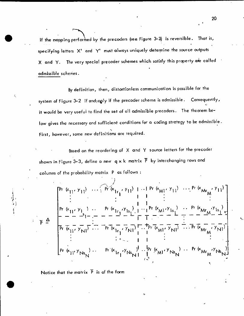
if t~e m~pping p~ed by the precoders ~ee Figure 3-3) is reversible. That is,
specifying letters XI and yi must always uniquely deter~ine the source outputs
X and Y. The very special precoder schemes which satisfy this property aJe called
admissible schemes.
By definition, then, distortionless communication is possible for the
system of Figure 3-2 if andT<>illy if the precoder scheme is admissible. Consequently, ~;
it would be very useful to find the set of ail admissible precoders. The theorem be-
low gives the necessary and sufficient conditions for a coding strategy to be admissible.
", First, however, sorne new definitions are required.
Based on the reordering of X and Y source letters for the precoder
shown in Figure,3-3, define a new q x k matrix P by interchanging rows and
columns of the probabil ity matrix P as follows :
Pr (x ll , Y1 ) s - - - -1-.-
1 .., Pr (x Ml' Y 11 )
1 1 , 1
Pr (x 1r 1 ' Y 1 s /. , ., 1 Pr (x Ml' Y 1 s 1 ) - - - - 1" T ,- - - --...----r+.----
Pr (x 1 r) , y N 1) 1 .. 1 Pr (xMl: y N 1 )
~ 1 1
Pr ' (x 1 ' YN )1 'Pr (x l' Y N ) r, sN 1 l 'M sN f .. ~
Notice that the matrix P is of the form
.• Pr (xM ' y 1 ) ___ rM _ s~ _
Pr (xM 'YNs ) rM N

P =
Pll 1 P21 1 .... 1 PMI 1 1 1 ---I--ï--ï---
P 12 1 P 22 1 .. .. 1 P M2 -;---r-:--j---,-:--
1 1 1 ----i--+---;--Pl N 1 P 2N 1 .... 1 P MN"
o
21
l '
where P.. IS the s. x r. matrix defined for i = l, 2, ... , M and i = l, 2, .•. , N Il 1 1
to be
Pr (xil' Yp) Pr (X. ,Y.I)
Ir. 1 1
Il P .. = Il
Pr (x'l'Y') Pr (X. ,y. ) 1 1" IS. Ir. IS. 1 1 1
Theorem 3-1: A precoder scheme is admissible for the system of figure
3-:-2 if and only if the corresponding matrix P as defined abQve has ot most one non-
zero element in eoch of its MN submatrices P .. , for i = 1, 2, ... , '1
M and i = 1, 2, .. , N.
Proof : Investigate the pre coder scheme illustrated in Figure 3-3 and its
corresponding probability matrix ;p : Consider any one of the submatrices P .. which Il
The r.s. entries of P .. are associated with the following r.s. (X, Y) 1 1 Il 1 1
pairs: (x il , yp), (xi2' yp) , .... , (x ir.' Yj1), (X il , Yj2) , (xi2 ' Yj2)' ..• , < 1
,)
(x. 'Y'2)' ... , (x.1
, y. ), (x'2' y. ), ... , and (X. ,y. ). But the precoder Ir. 1 IlS. IlS. Ir. IS.
1 1 1 1 1 of Figure 3-3 maps ail of the se (X, V) pairs onto the some (XI, VI) pair, nomely
• / '
22 -~-
. ~
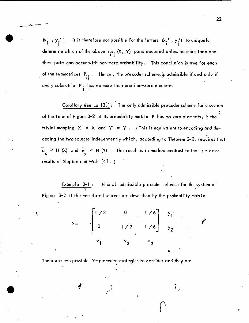
(x.' l y.' ). It is therefore not possible for the letters (x.', y. ') to unIque Iy 1 cil 1
determine which of the above r.s. (X, Y) pairs occurred unless no more thon one 1 1
1
these pairs can occur with non-zero probability. This conclusion is true for eQch
of the submatrices P ... Il
Hence , the precoder scheme<>lf admis,sibl_e if and on~y if , '
every submatrix P .. has no more thon one non-zero element. '1 '
Corollary (see Lu [3J): The only admissible precoder scheme for a system
of the, form of Figure 3-2 if its probobil ity matrix P has no zero elements, is the
trivi~1 mapping Xl = X and Y' = Y. ( This is equiva lent to encoding and de-
"
coding the two sources independently which, according to Theorem 2-3, requires that
n ~ H (X) and;;- ~ H (Y). This result,is in marked contrast to the E - error x y
results of Siepian and Wolf [4J . )
Example ç 1: Find 011 admissible precoder schemes for the system of
Figure 3-2 if the correlated sources are described by the probability matrix
r: 3 0 1/6] Y( " 1 P= 1/3 1 /6' Y2
Xl x2
x 3 f>
~ 0
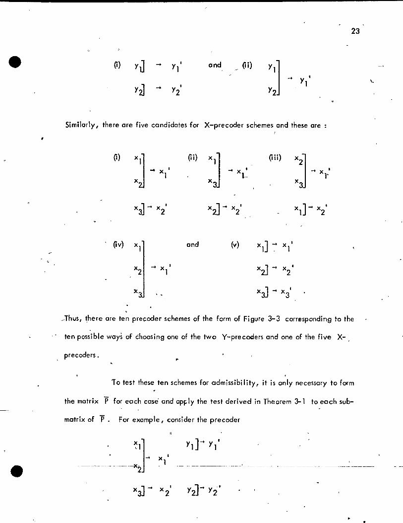
There ore two possible Y- pre coder strategies to consider and they ore , .'
~ /
r '.
23
0) yJ and Oi)
y~
Similarly, there are five candidates for X-precoder schemes and these are:
,
0) :j ~ Oi) Xl] o ii) X
2] • ~ x~ .... .
xl xl' x
3 x3
x~ ~ • x~ .... X • xl] ..... x2 ' x2 2
and (v)
~x' 1
..
~Thus, ~here are ten precoder schemes of the form of Figure 3-3 corresponding to the
- ten possible ways of éhoosing one of the two Y-precooers and one of the five X-
precoders. ..
10 test these ten schemes for admissibility, it is only necessary to form
the motrix P for each case and opply the test derived in Theorem 3-1 to each sub-
matrix of P. For example 1 consider the preceder
~1] -~-~--- ----- --x
2 ...
y ] ..... Y 1 1 1
1
xl -- -- --- -~-------~-- -- .~--------- ---
•
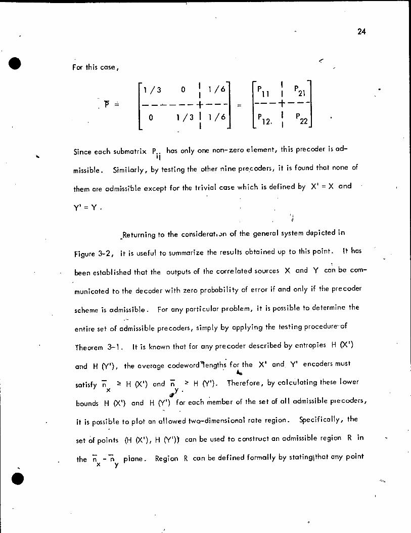
For th is case 1
1 /3 0 1 1/6 Pll 1 P
21 1 1 P - ------+--- = ---+---
0 1 /3 1 1/6 P 12. 1 P22 1 1
Since each submatrix P .. has only one non-zero element, this precoder is adI!
24
missible. Sîmilarly, by testing the other nine pre,coders, it is found that none of
them are admi.ssible except for the trivial case which is defined by XI = X and
yi =Y. '\ 4
.Returning to the considerat, .. >n of the general system depicted in
Figure 3-2, it is useful to summarize the results obtained up to this point. It has .
been establ ished that the outputs of the corre lated sources X and Y ca~ be com-
municated to the decoder with zero probability of error if and only if the precoder
scheme is admissible. For any particular problem, it is possible to determine the
entire set of admissible precoders, simply by applying the testing procedure"of
Theorem 3-1. It is known that for any pre coder described by entropies H (XI)
and H (YI), the average codeword"'ength~ for the XI and, yi encoders must . ...
satisfy n ~ H (XI) and n ~ H (YI). Therefore, by calculating these lower x y.
ri . H (XI) and H (Y') for each member of the set of ail admissible precoders, bounds
it is possible to plot an ollowed two-dimensiol'lol rote region. Specifically, the
set of points (H (XI) 1 H (YI» con be used to construct an admissible region R in
the n - n plane. x y
Region R con be defined formally by stotinglthat any point

"
25
CR ,R) must lie inside this area if and only if there exist encoders with x y ,
il == Rand n = R which allow the decoder to reconstruct the source outputs x x y y
with zero distortion.
The following two theorems are necessary for determining the admissible
region R in any general problem.
Theorem 3-2 Bit Stuffing : If the point (R 1 R) f R,' then the x y
point (R + 0 ,R + 0 ) f R for any 0 ,0 ~ 0 . x x y y x y
Proof : By definition, since the point (R ,R) f R, there must 'tJ, x y
exist on encoder havi ng n == Rond n ~R which allows the decoder to re-x x y y
'" construct the source outputs with zero probability of JIIIOr. .odify th is encoder as
follows : after every L1
codewords sent out by the X encoder, send Kl arbitrary
binary charaétefs ; similarly for the Y encoder, send K2
arbitrary bin~ry symbols J
after every L2
codewords. For this new coding scheme, the average codeword
lengths ore "x = Rx + Kl ILl and ny = Ry.+ K2 IL2 · The decoder con still re
. construct the source outputs :.vith zero distortion because it knows the numbers
K. , L. (for i = l, 2) and hence con count out sequences of L. codewords and 1 1 1
discard the following Ki meanin91ess binary symbol~. Therefore, the point
(Rx + Kl 1 LI' Ry + K2 / L2) f R where' KI' K2' LI' and L2 are any positive
integers. Any positive real number con be expressed as accl,Irately as desired os the (
ratio of two positive integ~rs by taking those integers to be sufficiently large. Con-
, 26
sequently, in the limit of large integers, KI/L1 and K2/l
2 can be replaced
by positive real numbers 6 and 5 . x y Thus, the poi nt (R + S,R + 5 ) ER.
x x y y
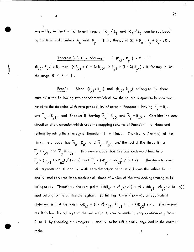
Theorem 3-3 Time Sharing :
(Rx2' Ry2) E R, then {À Rx1 + (1 - À) Rx2'
the range 0 :s: À :s: 1 •
If (Rx1' Ry1 ) E R
À Ry 1 + (l - À) Ry2}
and
E R for any À in
Proof : Since (Rxl" RyI
) and (Rx2' Ry2
) belong to R, there
must exist the following fylo encoders whi ch allow the source outputs to be communi-
cated to the decoder with zero probability of error: Encoder 1 having il = R 1 - x x
and n = RI' and Encoder Il having n ;. R 2 and n = R 2 Consider the con-y y x x y y
struction of an encoder which uses the mapping scheme of Encoder 1 u times and
follows by using the strategy of Encoder Il v times. That is" u / (u + v) of the
time, the encoder has ft = R 1 and il = R 1 and the rest of the time, it has x x y y
n = R 2 and n = R 2' This new encoder has qverage codeword lengths of x x y y
il = (uR l + vR 2) / (u + v) and "il = (uR 1 + vR 2) / (u + v). The decoder can x, x x y y y
still reçonstruct X and y with zero distortion because i~, knows 'the values for u
and v and can thus keep track at ail times of which of the two coding strategies is
being used. Therefore 1 the rate point «uRxI
+ vRx2
) / (u + v) , (uRyl
+vRy2
) / (u + v)
must belong to the admissible region. By letting À = u / (u + v), an equivalent
statement is that the point {ÀRx1
+ (1 - ~ Rx2
' ÀRy1
+ (1 - À)Ry2
) ER. The desired
result follows by noting that the ,value for À con he made to vary continuously From
o ta 1 by choosing the integers u and v to he sufficiently large and in the correct
ratio.

o
\
1 The above discussions have indicated that the admiss.ible rQ,te region
for any problem of the form illustrated in Figure 3-2 can be determi~ed by carry-
ing out the three steps summarized below :
0) Determine the set of ail admissible precoder schèmes with
the aid of Theorem 3-1,
." Oi) For eaçh member of this set, dete.,r;ine the lower bounds
H (XI) and H (YI) for n and' n respectively. Plot x y
ail these F*fnts (H (XI), H (YI» on the n -n pldne 1 x y
Apply Theorems 3-2 and 3-3 to the series of points
plotted-in (Ii) in order to disco~er the entire admissible Cl
region R.
This bosk method is best illustrated by apPIYi~ the solution of
several examples.
(continued) " "
For the probabi 1 ity matrix P =
the only admissible precoders were
o 1/6]
1/6 1/3
~
it was found that
()
o

28 /
e 1"
0) Xl] yJ ~ Yl ' Oi) xJ ... x' yJ'" Yl ' "'x' 1
1 and ./ x2 Yi] -0 Y2' x2J -. x' Y2] ....
1
2 Y2
x3J'" x2' xj] ... X 1
3
For scheme 0) it is necessary, that n ~ H (X') and n ~ H (Y') where x y
H (X') = - Pr (xl ') 1092 Pr (xli) - Pr r(x2 ') 1092 Pr (x2')
= - (2 /3) 1092 (2 /3) - (1 / 3) 1 0~2 (1 / 3)
= 0.918
and H (Y') H (Y) 1 1 1
1092
1 = = - '1 1092 '1 - , '2" = 1 .
,
For sche,me (Ii), it is necessory that n ~ H (X) = 1.585 and n ~ H (Y) = 1 . x y
These twoadmissible rate points (0.918, 1) and (1.585, 1) are
plotted in Figure 3-4. By applying Theorem 3-2, the admissible region R J is
found to include 011 po.nts of the form (0.918 + fi , 1 + fi ) for any fi , fi ~ 0 . x Y x Y
The resulting region shown in Figu~e 3-4 i.s actual Iy the entire admissible region.
It has such a simple shape that Theorem 3-3 does not yield any new information
about R .
Notice that if sources X 'and Y were coded independently, the ad-
missible region would be the double hatched region in Figure 3-4, the subset of
regio~) described by nx ~ H (X) and n y ~ H (Y) •
_ c.

l ,
rte •
n y
1 H(Y)t-----+J.......l.~~~~~~~
o .918 1.585 H(X)
"
Figure 3-4: The admissible region for- Example 3-1 .
n x
29
LI 30
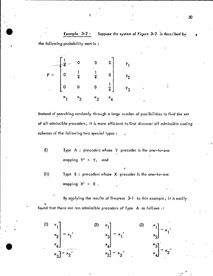
Example 3-2: Suppose the system of Figure 3-2 is describ~d by
" the following probability matrix :
1 0 0 0 YI
P = 0 l l
0 4' 4" Y2
0 0 0 l 4 Y3
xl x2 x3
x4
Jnstead of searching randomly through a large number of possibilities to find the set " .
of ail admissible precoders, it is more efficient to first discover ail admissible coding
schemes of the following two special types:
(1) Type A ; precoders whose Y precoder is the one-to-one
mopping yi = Y, and
(Ii) Type B ; precoders whose ~ precoder is the one-to-one
mopping XI = X .
By applying the results of Theorem 3-1 to this example, i t is easily • 1
\f ù
found that there are ten admissible precoders of Type A as follows :'
(1 ) Xl (2) Xl (3) Xl ' • Xl "'x l ... X 1 x
2 l x3 1 x
2
-e x4
x4
X
J ---- ... X 1 ]-+ X 1 x2] - x 1 X 2 x3 2 2

31 t. ,~\
- (4)
:J~ (5) Xj (6)
X~ Xl .... X ' X ... xl' 1 ' 1 X
X2] ~ , x2J .... x2' xj] .... x2 ' x2
x4 xj] .... x
3' x] .... X '
4 3
(7) xl] .... x ' (8) XJ
(9) x]- X ' 1
x ... xl' 1 1
x2] .... x ' 2 Xl X '
x2J .... x2' x4
2
X3]
.... x' x
4] .... x
3' xaJ - x3' x
4 3
'lI" f'
~
xl] - xli ,
X ] .... 2 ' Xl
2 -'
'x~] ... X '
r .~ 3
x4] .... x ' 1 4
.,.. QI course, the Y precoder scheme in each of these cases is understoo~ to be the
trivial one Y' = Y . .,.
i
Similarly, it is easily found that there are five admissible precoders
~ of Type B ,as follows :
..

e
1.
{
32
(1) (2) (3) Y1 Yl YI] .... 1
Y3 .... Y1' Y2 .... y' Y2 Y1 1
" Y3 y3] .... Y2 1 Y ] ... Y 1
2 2
(5) Y1] - Y1 ,
.Y2] .... Y , 2
Y3] .... Y3'
/ It is understood that the X precoder in each of these cases is defined by X' = X .
As illustrated by this example, the set of ail admissible Type A pre-
'coders is actually a list of X precoder schemes. Si"1ilarly, finding ail admissible
Type B precoders gives a list of Y precoder strategies. The significance of these
, >
two 1 ists is that any pre coder of the general form of Fi gure 3- 3 can only be ad-
missible if its X precoder belongs to the Type A list and its Y precoder belongs 'l
to the Type B list. In other words, if the. precoder of Figure 3-3 is admissible,
the two precoders shown in Figure 3-5 must alst> be admissible. This fact becomes ~ 1
obvious according to Theorem 3-1 by inspecting the P matrices correspondipg to
the three precoders in question.
f method, then, to determine the set.t>f ail admissible Pl-'écoders in
• any problem, is to consider ail possible ways of choosing an X precoder From the
<)
Type A list and a Y precoder From the Type B list and to apply the test of
Theorem 3-1 to each of these possibilities.
-,
~

~ .. 7
"
xl1 x12
;;:,. X 1
~ - 1
x lr1
x21 x22
... x 1 2 '
x2r
- X 1 M
X MrM
YI]
Y2]
Y3]
J-
(a) A Type A precoder.
...
...
...
1
YI
1
Y2
Y3 1
yi q
Figure 3-5: Type A
7
--1-1r f: ~_ .-1 .~
~Y12 '. -
.. ... 1 "".' ~1-
Y1s 1
; ,Xl] ... X 1
1
~21 x~ . ... X 1
2 Y22
x 3] ... x 1
3 ... Y2
1
Y2s
. . '
... X 1
k
(1)) A Type B precoder.
,tl B precoders.
33
"
l
(
34
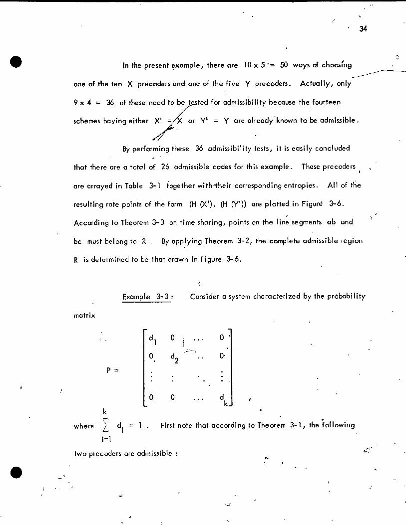
ln the present ~xample, there are lO x 5 . = 50 ways of choosfng -------one of the ten X precoders and one of the five Y precoders. Actually, only
9 x 4 = 36 of the se need to be t ted for admissibility because the fourteen
schemes having either XI = or yi = Y are already"known to be admissible.
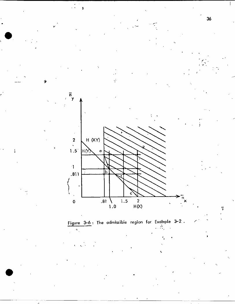
By performing these 36 admissibility tests, it is easily concluded
that there are a total of 26 admissible codes for this example. These precoders 1
are arrayed in Table 3-1 together with1'heir corresponding entropies. ALI of the
resulting rate points of the form (H (XI), (H (YI)) are plotted in Figure 3-6. ,
According to Theorem 3-3 on time sharing, points on the line segments ab and
bc must belong to R. By applying Theorem 3-2, the complete admissibre region ,
R is determined to be that drawn in Figure 3-6.
Example 3-3: Consider a system characterized by the prôbability
matrix
dl 0 0 , 1 _
0 d2
,:::~,
O·
P =
0 0 d k
k \'
where L d. = 1 . First note that according to Theorem 1
j=l
two precoders are admissible:
• 3-1, the forlowing
.,' <-.

35
" .. Precoder No. X Precoder No. Y Precoder No. H (X') H (Y')
"",j~I'"-- .' -, ) -
'10 1 2 ..0
2 10 2 2 .811
3 10 3 2 1
4 10 .tf. 2 .811
5 <, 10 5 2 1.5
',<
6 L' 9 2 1.5 .811 J ,
7 <. ; 9 - • f 3 1.5
8 9 5 1.5 1.5
9 8 3 1.5 [.
10 8 4 1.5 .811 , ,
11 8 .5 1.5 1.5
12 7 2 1.5 .811
1~ 7 3 \ 1.5 1
14 7 5 1.5 1.5' . 15 6 3 1.5 1 " r -16 6 4 1.5 .811
;
17 _l, 6 5 1.5 1.5 , ! '" f "-,,, ..
d 18,_ '. 5 2 1.5 .811 --,
19 5 '. 4 1.5 .811
20 5 '5 1.5 1.5
21 4 3 1
22 4 5 1 1.5
23 3 3 1
24 3 5 1 1.5
,25- 2 J
5 .811 l.S
26 5 .811 1.5
e ) Table 3-1 : The admissible precoders for Example 3-2.
e,
,-
. ..
\01'
"
n y
2
1.5'
'1
,.
. 811 ........ -_-+=~~--fI_~ ....
1 ) \ ,
o .8l 1.5 1.0
2 H(X)
" "
"
n x
.:
Figure 3-6: The admissible region for Example 3-2. ,/ ,',
" '. " .
36
.,. l" 0
, ... ' ( ~'f' •
_ 0
\ '
"

"
37
(1 ) Xl yJ ~ yll (2) xJ ~ XII ..yI
x2 y~ ... y 1
2 x2J ~ X 1
2 Y2 ... x 1 and ... 1
1 YI ,~ YJ ... Yk ' xJ'" xk
' xk' Yk
Thefe.fore the po~nts (0, H (Y)) and (H (X), 0) belong to the QdmissibL~ r~9ion R.
Notice that since P is diagonal, H (X) = H (Y) = H (XY). The two points
. . (0, H (XY» an~ (H (XY), 0) are plotted in Figure 3-7. The following theorem
allows the adl')'lissible region for this example to be dete~mined by inspection.
Theorem 3-4: For a system of the form of Figure 3-1 1 (or L\ Figure 3-2) the source outputs con be communicated to the decoder with zero
probability of error only if o' + ri ~ H (XY) .. X Y
Proof : Suppose a system exists which allows the' source information
to be communicated to the decoder with Zero distortion and whith has encoders such
, that ri + iï < H (XY) . Consider a co":,bining of the X and Y encoders of this X Y
4' system to form an XY encoder for the ioint source XY. For examp le, choose an
XY encoder which alternates on every bit between the codeword sequences of the
X and Y encoders.' This encoder allows the decoder to reconstruct the output of ,
source XY with zero distortion and furthermore, it has an average codeword length
of" =n+n xy X Y
Therefore, n < H (XY). However, according to Theorem xy
2-3 for the single source XY 1 it is' necessary that n ~ H (XY) .,.in order to have xy
distortionless communication. This contradiction implies that the opening assump-

. 1
cl
•
n y
o )
=----"---~ -
.H (XY)
figure 3-7 ~ The admissible r,egion for Example 3-3 .
n x
'.

\
,
tion was wrong. Therefore, no system can exist with n + n < H (XY) such x y
that the source outputs ca~ be reconstructed by a decoder with zero p(obability
of error. That is, it is always necessary that n +n ~ H (XY) . x y
39
'", Example 3-3 (concluded) ln Figure 3-7, the line segment joining
the points (0, H (XY)) and (H (XY), 0) is the line n + ri d: H (XY) . x y
. Aàording
to the Time Sharing Theorem, points on this segment are admissible. Theorem 3-4
proves that no points below this line con belong to region R. Therefore, the entire
admissible region R is that i1lustrated in Figure 3-7.
This chapter has developed sorne simple procedures for finding the ad-
~ missible region R for problems of the form indicated in Figure 3-2. Until now,
, \'hj, ho, been a re,,;jcted cio" of problem, becou,e 'h"~recoders have been limited
''').
to performing transformations oh the individual source leUers. Fortunately, it is very . '
easy to generalize this situation to allow coding for sequences of source letters. In-
deed, by pretending that the X source letters xl ' x2
' .. , xk
and the Y source
letters Yl' Y2' ... , y are actually sequences of L leHers From two simpler q ,
sources, the most .general problem con be solved using exactly the sorne methods em-
ployed previously in this chapter. This fact is illustrated by the following
concluding example.
Exomple 3-4
by the probobility matrix
Find the admissible region R for a system described
1. 1 ":.
f •

---------~-
40
e. 1/3'
0 1/6] YI P =
. 0 l /3 1/6 Y2 - ='
xl x2 x3
if coding4
is permitted for sequ'ences of L = 2 source Jetters .
By assuming that source X actually has 9 outcomes xl xl l ,
xl x2 ' xl x 3, .•• , x3 x3 and source y has four letters Yl Yl ' Yl Y2' Y2 Yl' P'
and Y2 Y'2' .the following equivalent problem can be set up: find the admissible
regi.an for a system with probability matrix
1/9 cl 1/18 0 0 o --- 1/18 0 1/36 Yl Yl !
0 1/9 1/18 0 0 0 0 1/18 1/36 Yl Y2 P =
0 0 0 1/9 0 1/18 1/18 0 1/36 Y2 Yl
0 0 0 0_ 1/9 1/18 0 1/18 1/36 i , '. Y2 Y2 ,.
x1x
1 x
1x
2 x
1x
3 x
2x
1 x
2x2 x
2x
3 x3x) x3x
2 x3x~ .. ;
if coding is only permitted forJndividual source letters. 0
It has been establis:,ed in this chapter how to solve such a problem.
It turns out in this case that no admissible Type B precoders exist besides the trivial
one but that othe best ' (Iowest entropy) admissible Type A pre coder is the code

• -- - -- --------- - ~
41
"
L ,
,
whichhas H (XI) ;" 1(0.91') and H (YI) = 2 (1). Therefore, the point . '
iï = H (XI) /2 = 0.918 arid iï = H (YI) /2 = 1 is an admissible rate point, x y .
the extra factor of hvo arising because the above preceder is fer seque~ces of length
twe. Consequently, the ad~'issible region R is the same as tha't plotted in Figure
3-4 in connection with Example 3-1 .
o
'.
«,'

42 '
CHAPTER IV
AN ALGORITHM FOR DETERMINING THE }DMISSIBLE REGION
Ali th~ basic ideas and theorems necessary in understanding the system
of correlated sources illustrated in Figure 3-2 have been established in Chapter III.
ln practi ce 1 however 1 the soluti on of problems described by large, sparse probabi 1 i ty
matrices can require an enormous amount of work. For example, for a system with
a 10 x 10 probability matrix, there ore many billions of different precoder mapping
combinations of the form of Figure 3-3. To search randomly through this gigantic
number of possibilities to find the admissible coding schemes iS.Qbviously imprae>tical,
if not impossible. The purpose of thi.s chapter, then, is to develop an algorithm
which allows such large problern.s to be solved efficiently with the aid of a digital
computer. It should be kept in mind that even though the methods below assume that
only coding for individual source letters is permitted, they con be applied equally
weil to problems allowing coding for sequences.
During the discussions of Chapter III and specifically in connection
with Example 3-2, the following four step method was suggested for solving any . ,
correlated source coding problem of the form of Figure 3-2:
Step A: Determine the set of 011 admissible precoders whose Y J
precoder is defined by the one-to-one mapping yi = Y. Eaèh admissible code of
this restricted type, which we shall cali Type A, has a different X precoder. The
result of Step A, the/, is a list of various X precoder mapping schemes. ,
"

43
Step B': Determine the set of 011 admissible precoders whose X, ,
precoder is defined by the one-to-one mappin~ XI = X. Each admissible code of
this restricted type, called Type B, is characterized by a different Y precoder.
Therefore, this step results in a list of various Y precoder mapping strategies.
Step C: Consider the set of 011 possible ways of choosing an X
precoder from the Iist discovered in Step A and a Y precoder from the list found ty
in Step B. Test each su ch precoder for admissibility. As proven in Example 3-2,
this procedure determines the set of 011 admissible precoders.
Step D:
culate and plot the points
For each admissible precoder revealed by Step C, cal-
(H (XI), H (YI)) on the n - ri plane. x y
Find the entire
admissible region R by applying Theorems 3-2 and 3-3.
The above four steps form the basis for an algorithm which will be
developed in the remainder of this chopter. First of ail, a detoiled strategy will
be given for efficiently performing Step A. No new methods will be necessary
for Step B because it only differs from Step A in that the roles of X and Y are
reversed. An improved final step will then be worked out by combining Steps C
and D. This procedure wi 1\ tc.:ke advantage of the fact that in most problems, it
is not necessar'y to determine the complete 'set of admissible precoders (as in Step C
obove) in arder ta draw the admissible region R. For instance the admissible region
drawn in Figure 3-6 in connection with Example 3-2 is defined by only three pre-
------------ ---- -- - -----------

44
coders, those corresponding to the points a, b, and c. Non~ of the other ad-
missible precoders appear in the final solution.
Aigorithm for Step A: Consider a problem of the form depicted
in Figure 3-2 which is characterized by a given probability matrix P. The goal
of Step A is to use this given information to discover the set of 0" admissible pre-
coders of the special type (fype A) shown in "Figure 3-50. Notice that the Y
precoder is limited to be a one-to-one mapping whereas the -x precoder is un-
restricted. It is convenient to divide the set of 011 admissible Type A precoders
i~fferent clos"ificatio:s bosed on the i r X precoders. Specificdlly, catagorize
t~coders accdrding to how many groupings of two or more X source letters
occur in the X precode";mapping scheme . For example, for the precoder of "
/~--) Figure 3-5a, if rI' r 2 1 ••• , rJ are 011 greater than one and r J+l ' r J+2 1 ••• , r M
ore ail equal to one, then this X precoder has J groupings of two or more source
letters.
This classification for Type .A precoders indicates that Step A can
be carried out in severo 1 sequential steps a~ follows :
l' .. --: Step A (1) Dete.rmine the set of 011 admissible Type A precoders
whose X mapping sch~mes have at most one groLlping"Of two or more source letters.
, ,
i. »

45
Step A (2) : Determine the set of 011 admissible Type A precoders
whose X mapping schemes have two gfoupings of two or more source letters.
Step A (J) : Determin~ the set of 011 admissible Type A precoders
whose X mopping schemes have J groupings of two or more source letters.
By choosing the number J to be large enough, the sets 9f admissible
precoders found in Steps A (1) through A (J) together make up the set of 011 ad-
missible Type A precoders. The advantage of performing Step A according to
this sequence of J steps is thot it turns out that once Step A (1) has been completed,
"', Step A (2) con be performed directly from the results of Step A (1) without even
• looking at the probability matrix. Similarly, it will be shown below how ony Step
A (J) con be corried out directly from the results of Step A (1-1) by 0 simple pro-
cedure.
The key, then, to efficiently performing Step A occording to the set
of steps indicoted above is to develop ,!n algorithm ta car~y out Step A (1). This in-
volves discovering tf)e set of ail admissible precoders of the special form illustrated in
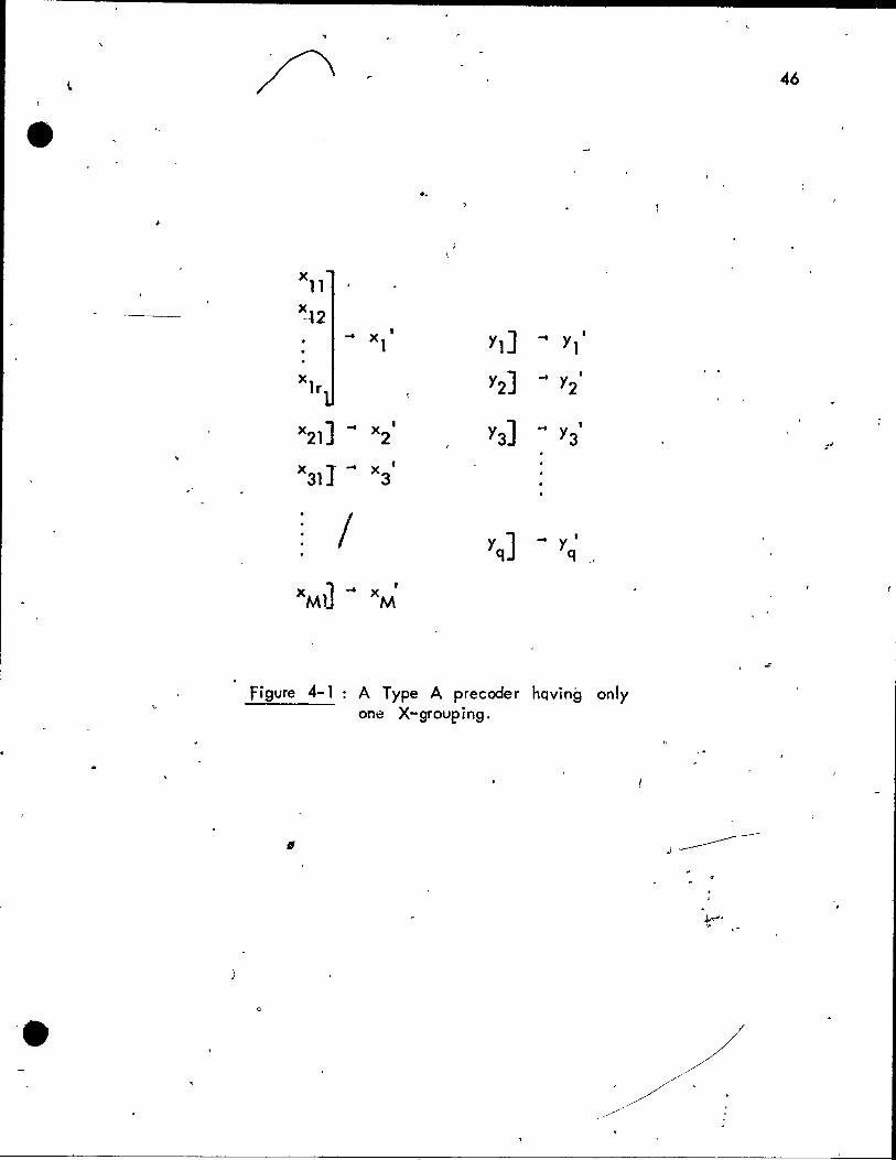
Fi,gure 4-1. These codes are cha:acterized by X mopping schemes having either one
grouping of tW\,Q or more source letters (when r 1 > 1) or having no such groupings
(when r1
= 1). For any admissjble precoder of this form we will henceforth refer to
its only grouping of source letters (xl1
1 x12
' .... , x1r1
) as being an admissible X-
<,/
..
Xll
~l2 .... x '
1 Yl] ... Yl'
x1r Y2] .... Y2'
x21 ] ... x • 2 Y3] .... Y3'
x31 J .... x • 3
1 Yq] .... y ,
q
xMtl .... . x
M
Figure 4-1 A Type A precoder hQving only one X-grouping.
Il
46
~A
. ~.

f\
/
47
~ grouping. Using this terminology, the gool of Step A (1) can be restate'd as follows ;
-. .... .. ." ,
Il
find the set of ail admissible X-groupings .
• To ach~eve this objective, consider the forming of a matrix Po by per-
forming column interchanges on the probability matrix P according to the following
rules 1
P = 0
,
(r) Find the row of P which has the most non-zero entries :
th the JO row. If two or more rciws have the same maxi-
mum number of non-zero entries, choose any one of these
1 . rows. 'pefine 10 to be thé number of zeroes in the
th JO row.
th (ri) Interchange columns of p' so that the JO row has ail of
Y,
YJ . 0
Yq
, , . its 10 zeroes in the leftmost columns.
The resulting matrix ! 0 has an appearance of the following form
.. 1 1 1 A
0 0 0 1 x x X :::i [POl 1 1 .1 1
, 1 01 01 01 02 02 02
x.- x2 XI x, x
2 x
k_
1 : 1 0 0
.p 02] ,
where "x" denotes a non-ze"r,o element. Notice that Po has been partitioned into
"two matrices' POl and P02
and the X source .etters have been relabeled àccordingly.
=

48
Since each column of P 02 has a non-z~ro eler;nent in the Joth
row, Theorem 3-1
implies that any precoder of the form of Figure 4-1 cannot be tOdmissible if the X-,
grouping (xll,'x 12"' ..• , x 1r 1) contains two or more of the source letters
02 02 02 xl" x2 ' .. '., and xk _
1 . In other words, anyadmissible X-grouping for the
~ 0 system described by matrix P
02 02 none €Jf the letters xl ' x
2 '
(or equivalently PO)' must contain only one or else
02 ... , x
k_
1 o Consequently, Step A (1) can be
solved by combining the solutions of th~ following two simpler problems:
(1) Find the set 51 of 011 admissible X-groupings wh ich
02 02 contain none of the source letters xl ,x
2 ' ... , and
02 xk_
1 o and
(II) Find the set :12 of 011 admissible X-groupings which
02 02 contain exactly one ';f the source letters x
l-, x
2 ' ... ,
02 and x
k_
1 o
/
U"
It will now be shown how these two steps can be used as a basis for
a recursive algorithm for carrying out Step A (1) .
• 1
I~
\:.-. , , 1 . -~~
",
First of ail, consider the first step, problem /,. It involves the study
of X-groupings which cont'ain only source letters associated with matrix POl J
01 01 01 namely Xl 1 x2 " ... , XI But the set of 011 admissible X-grol-'pinfls of this
, 0 type is just the set of 011 admissible X-groupings f<;>r a system of the form of Figure
3-2 which is described by the probability matrix POl instead of Po Therefore,
'.
"
..
49
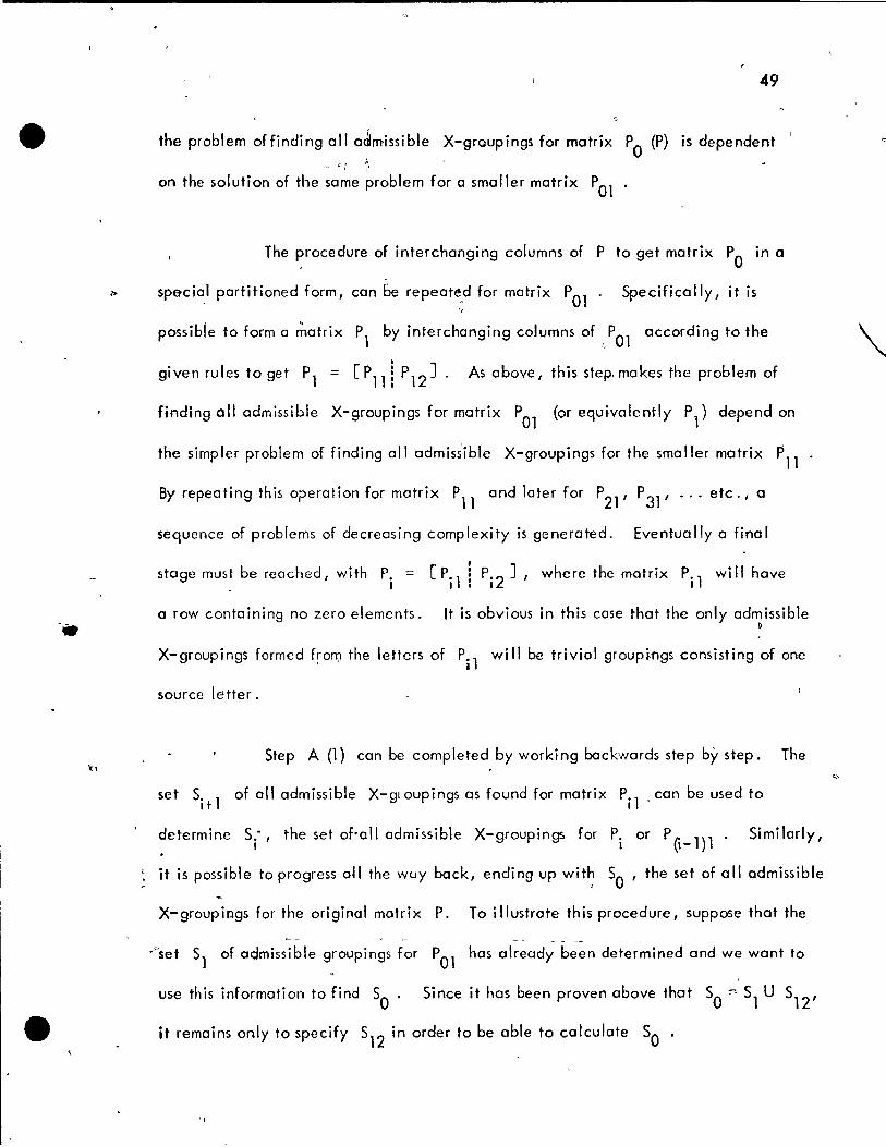
the problem offinding ail a~missible X-groupings for mafrix Po (P) is dependent " . .
on the solution of the ~a~e ~roblem for a smaller matrix POl
The procedure of interchanging columns of P to get matrix Po in a
speci~1 partitioned form, con be repeaté,d for matrix POl Specifically, it is "
possible to form a ~atrix Pl by interchanging coJumns of ,-POl according to the
given rules to get Pl = [Plll P12]. As above, this step.makes the problem of
finding 011 admissible X-groupings for matrix POl (or equïvalently Pl) depend on
the simpler problem of finding 011 admiss'ible X-groupings for the smaller matrix "11 By repeating this operation for matrix PlI and later for P
21, P
31, ... etc., a
sequence of problems of decreasing complexity is generated. Eventuallya final
stage must be reached, with P. == [P.l! P'2 J, where the matrix P., wi" have
• 1 1 : 1 1
a row containing no zero elements. It is obvious in this case that the only admissible ~
X-groupings formed f~on;J the lefters of Pjl will be trivial group~11gs consisting of one
source letter.
5tep A (1) con be completed by working backwards step by step. The
set Si+l of 011 admissible X-gloupings os found for motrix Pil
,con be used to
determine \-, the set of-ail admissible X-groupings for Pi or P (i-1)'. 5imi larly,
, if is possible to progress al! the wuy bock, endi ng up wit~ 50' the set of a Il admissible
X-groupiogs for the original matrix P. To illustrote this procedure, suppose that the
·'>-set SI of oc;Jmissible groupings for POl has olready been determined and we wont to "
use this information to find SO. Sin.c;e it hos been proven above thot 50 = 5, U 5'2'
it remains only to specify 512
in order to be able to calculate 50 .
"
50
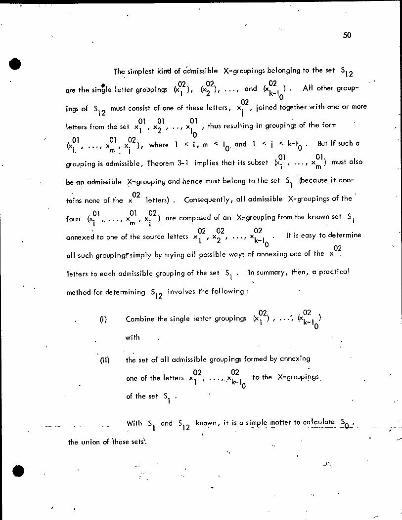
Th~ simplest kirfd of a'dmissible
h • -1 1 • (x02 )' ( 02)
X-groupings belonging to the set S12
02 ... , and (x
k_
1 ). Atl other group-qre t e smg e etter grocrplngs l' x'2 '
o ings of 5
12 must consist of one of these letters, x~2, joined together with one or more
1 f h 01 01 01 hl" .' f h f etters rom t e set xl ,x2
' .. , xI ,t us resu tmg ln groupmgs 0 t e orm
01 01 02 0 (X. , .•• , x ,x. ), where 1 ~ i, m ~ 10' and 1 ~ j ~ k- to" But if such a
1. m. 1
• . d" b 1 Th 3-1' l' h . b (x01 01) 1 grouplng IS a missI e, eorem Imp les t at Its su set ., ... , x must a so
1 m ,
be on admissible , ?<-grouping and hence must belong ta the set 51 (because it con-
t-ains none of the 02 x letters). Consequently, ail admissible X-groupings of the
01 01 02 • form (x. , .... , x , x. ) are composed of an Xrgrouplng from the known set 51
1 ml, . m m ~
onnexed to one of the source letters Xl ' x2
' ... , x k_1
. It is easy to determine o
ail such groupingrsimply by trying ail possible ways of annexing one of the x02
letters to each admissible grouping of the set 51' In summary, then, a practical
method for determining 512
involves the following :
r.) b h 1 1 . (x01
2) " (x02 ) ,1 Com ine t e sing e etter grouplngs , ... , k-I
° with "
Oi) the set of ail admissible groupings formed by annexing
02 02 one of the letters Xl ' .•. ",x
k_
1 to the X-groupi!"9S"
° of the set 51 .
~ith 51 and 51-2- kn~ ..... _n, it is a si~ple fl')atter to ca!~u~ate __ ~~-' _
the union of 'these sets\.
"
51
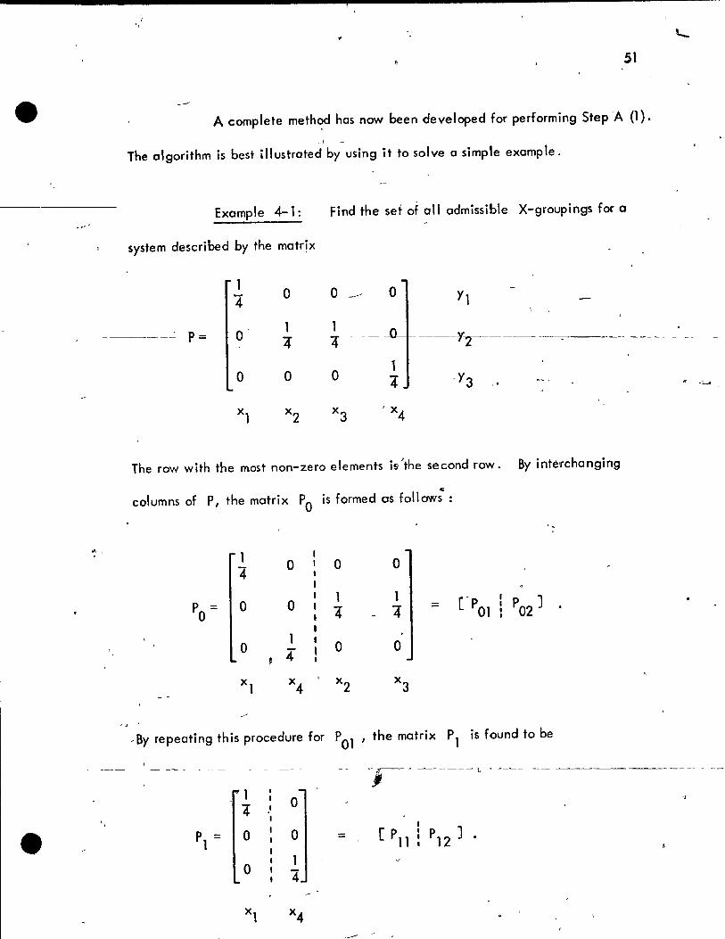
A complete meth~d has now been developed for performing Step 'A (1).
The algorithm is best illustrated by using if to solve a simple example.
Example 4-1: Find the set of 011 admissible X-groupings for a
system described by the matrlx
1 0 0 "4 ---' y,
p;; 0 1 1 4' 4' ---~-Y-r-----
0 0 0 l '4 -Y3 ,-
Xl x2
x3
'x 4
The row with the most non-zero elements is 'the second row. By inté'fchanging
'" columns of P, the matrix Po is formed as follows :
, .
~ , , 0 0 0
"4
P = 0 0 1 1 [-p 01 P
02 ]
"4 "4 = 0
0 ,
0 0 4"
x, x4
x2
x3
. -By repeating this procedure for PO' ' the matrix P, is found to be
- ~- --"-- -
, 0 '4 1
1
P = 0 1 0 = 1
0 1 "4
J
Xl x4 . .-'
..
/ , f~ . , .'
52
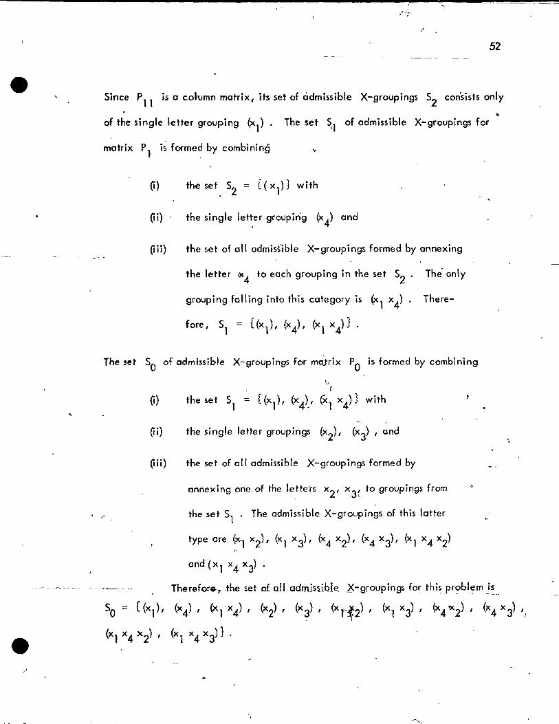
Since P 11 is a column matrix, its set of àdmissible X-groupings S2 consists only
of the single letter grouping (xl) .
ma tri x P 1 i~ forme~ by combining
The set S'lof admissible X-groupings for
(ii) 1 the single letter grouphlg (x4) and
(iii) the set of ail admissIble X-groupings formed by annexing
the letter "'4 to ea,ch grouping in the set 52' The' only
grouping falling into this category is (xl x4). There
fore, 51 = [(xl)' (x4)' (xl x4)} .
The set So of admissible X-groupings for majrix Po is formed by combining
',. i
(i) the set 51 = [(xl)' (x 4).' (xl x 4)} with
(ri) the single letter groupings (x2), (x
3), and
(iH) the set of 011 admissible X-groupings formed by
annexing one of the le,tte'rs x2 ' x3~ to groupings From
the set 51 • The admissible X-groupings of this latter
type are (x, x2), (xl x 3), (x4 x2), (x4 x3L (xl x4 x2)
and (xl x4 x3) .
..
---- - ~- --~~~~-~ ~ Therefore-, -the set -of olLcdmiss.ible __ 2<-groupings for thj~ pr~bl~m i~_
So = (xl)' (x4)' (xl x4), (x2), (x3)' (xr~2)' (xl x3) 1 (x4 'x2), (x4 x3) '/
(xl x4 x 2), (xl x4 x3)}
53
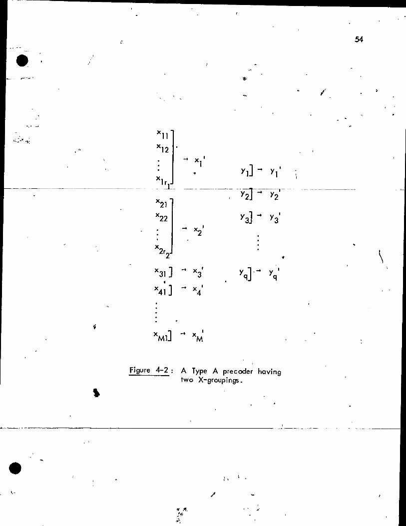
Now that an algorithm has been developed for 5tep A (1), let us turn
our attention to,5tep A (2), the problem of finding 011 admissible precoders of the
type illustrated in Figure 4-2 (where rl
' r2
> 1), Notice that if the precoder
of Figure 4-2 is admissible, then according to Theorem 3-1, the X-groupings
(Xll
,x12
, "" xlrl
) and (x2l
' x22
' "" x2r2
) must be admissible by them,
selves and thus must belong to the set 50' Consequently 1 it is possible to carry out
Step A (2) dir~ctly from !he results of 5tep A (1) as follows: take the set 50 of
admissible X-groupings found.in 5tep A (1) and try 011 possible ways of çombining
two of these groupings to form precoders of the form shown in Figure 4-2,
Examp le 4-1 : (continued) It has been found above that the set of
011 admissible X-groupings is 50 = [(xl)' (X4
) , (xl x4), (x 2) , (x3), (xl x 2),
(xl x3), (x
4 x
2), (x
4 x
3), (xl x
4 x
2), (xl x
4 x
3)} , To find ail precoders having
the form shown in Figure 4-2, we need only investigate ail possible ways of choosing
two From the following X-groupings ~ (xl x4), (xl x
2), (xl x
3), (x
4 x
2), (x4 x
3),
(xl x4 x2), (xl x4 x3)
Forming a pre coder from the two groupings (xl x4) and (xl x2) is
clearly unacceptable because the I~tter Xl appears twice 50 that an X-mapping
scheme is not weil defined, Similarly, choosing the grouping (Xl x4) along with
any other does not form an acceptable precoder, By trying 011 the other possibilities,
it is easily found that the following are the only two admissible precoders of the re-
quired type:
----------------------------................. . 54
.. , ~ _-.#
ya ... Yl \ "
.... X 1
1
x1r
--------------[---- - ----~-~ --Y2r=.--Y2r -···-------------
x21
------------------------
\.
x22
... X 1
2
... X 1
3 ... X 1
4
y 1
q
Figure 4-2: A Type A precoder having two X-groupings.
\ l'
, " .!fI
\

el "
55
Xl] xl ] .... x l .... X 1
x2
1 x3
1
and
X3] ~ 1 X2 ] ~ Xl x2 2
x4
x4
Consider now a method for performing Step A (J) given the results of
Steps A (1), A (2), ... , and A (J-1). The goal is to determine 011 admissible pre-
coders of the form shown in Figure, 4-3, where r l' r 2' .... , r J are a1l restricted
to be larger thon one. ~ According to Theorem 3-1, if the precoder of Figure 4-3
isadmissible, 011 of the X-groupings (x 11 , x 12 ' ... , x1rl
), (x21' x22 ' ... , x2r2
)' .... ,
and (1< JI' x J2' ... , x Jr} must be admissible by themselves and therefore must be-
long to the 1 ist found in Step A (1). Furthermore, any precoder formed by choosing
any (J-1) of the J X-groupings o"f Figure 4-3 must be admissible and thus must be-
long to the list of admissible precoders found in Step A (J-l) .
Hence, a method for finding the set of ail admissible precoders of the form 1
in Figure 4-3 is to investigate 011 possible w9Ys of a~nexing one of the admissible X-
groupings found in Step A (1) to one of the admissible precode.rs found in Step A (J-1).
Example 4-2: Find ~he set of 011 admissible Type A precoders given 1
___ ------' _th_a_t_ t~e' outcome of Step A (1) (the set of 011 admissi ble X-groupings) is the set
So = [(xl x2), (x 3 x4),
(x4) , (><5), (x6)}·
-. r

o
j
"'"
~f" :<
xll .-
'il x12 :-~--~ -~~~-~~-- ~~----~~-~-- -~--' _____ '_, - ..... _~>41 _. _____ ~_~
.. '
~ ',-
<:l 'i
. -
.. x ~ 1r
l
x2l
x22 Yl]
... X 1
2
x 2r2
Y2T
Y3]
~. xJl
xJ2 ... Xl
J'
xJr Yq]
1 ..... X J +1
xMil ..... 1
xM
Figure 4-3: A TYP,e. A precoder having J X- groypings.
• 0
... Yl '
... Y2
1
... Y3
1
... y 1
q
-, , .
56
. ,
, ,
•

.P
57
st:p A (2) By trying each possible way of choosing two of -the
X-groupings From the ,set 50' (excluding'the trivial groupings (xl), .(><2)' ... , (x6», the following precoders are found to be admissible:
Xl ] ~ , X~] ... X ' x3] -t x '
x2
xl x2
1 x4
1
X3] X5] '-. X5 ]
"xq .... X ' ... X ' -t X ' 2 x
6 2 x
6 2
~---
x5J .... x' 3 x3J "'x'
3 xl] ... x ' 3
x6J -t x ' 4 x4J ..... x' 4 x2J ..... x''
4
Xl]" Xl] ..... )<' x2 ] .... x ' x .... x' l " 2 1 x3
1 x3
x3
X5] 'x5 ] , "'x' .... x2
x5 ] x
6 x
6 2
... x ' x
6 2
x2J ... , xlJ .... x' x
3 3 x4 J-t x ' x4] ... x' x4 J .... x"
3 4 4
~
5tep A (3) : By trying each possible woy of annexing one of the X-
groupings of the set So to one of the six admissibl~ precoders found in $tep A (2), ;
the following precoder is found to be the only admissible one
X ' 3
l'
'.

58
There are no precoders containing more thon three X-groupings of more
thon one source letter. Therefore, the set of 011 admissible Type A precoders is
formed by combining the admissible precoders found in Steps A (1) 1 A (2), and A (3).
The algori,hm developed above for performing Steps A (1) through A (J),
allows the determination of 011 admissible Type A precoders as required by Step A. '
The methods are very weil suited ,for computer programming due to the simple step by
step progression. Some more examp'ies will be presented towards the end of this
chapter to illustrate how efficiently the above method can be implemented by a com-
puter program.
Aigorithm for Step B: l The object ~f Step B is to determine the set of
011 admissible Type B precoders. This is exactly the same problem as solved in Step A
except that the roles of X and Y are reversed. Therefore 1 the identical method de-
veloped above can also be used for Step B simply by replacing the probability matrix P
by i ts transpose pT
Aigorithm for Steps C and D: The goal of this final step is to determine
the admissible region R given the set of 011 admissible Type A and Type B pre-
coders as found in Steps A and B respectively. The list of admissible Type A
precoders is actually a list of KA different X precoder mapping schemes and si~ilarly,
the set of adrnissibl~Î Type B prec'oders is a I~st of KB
Y precoder mapping schemes.
The set of 011 admissible precoders is thus a subset of the K AKS different possibre ways /
/

i 1 -
59
of ch?osing an X precoder from the Type A list and a Y precoder from the Type
"" B list. As shown in Figure 4-4, each of these K AKS possibil ities dèfines a point
(H (X'), H (Y'») in the n - -;) plane. Therefore, the proble'm of determining the x y
admissible region R involves searching through a"grid of KAKB
points to find which ,.
ones, (out of those corresponding to admissible precoders) are the vertices defining
region R.
Many of the grid points in Figure 4-4 can be eliminated From further
consideration by inspection. For example, "as proven by Theorem 3-4, none of the
grid points below the line n + ri = H (XY) (which is th~ line FG in Figure 4-4) x y
can represent admissible precoders. Furthermore 1 since points C and D are known
to represent admissible precoders (of Type A and Type B respectively), ail of the
grid points above the line segment CD must lie insfde the boundary of the admiss.ible
region R, as proven by Theorems 3-2 and 3-3. Consequently, it can he stated ,
that no points other than those Iying on or between lines CD and FG can be ver-
tices for region R ,
A method, then, for discoverfng the admissible region R, is to
systematically choose points from the area hetwecn lines CD and FG, ~nd to test
" i tM correspondinQ prec3ders for admi~0ibil ity. Whenever a code is testea andlound
()
" to he admissible, the region R can be increascd accordingly. For example, if the
code corresponding t-o"point E of Figure 4-4 is found to be admissible, the triangu-
lar area CED can be added to R. Moreover, only the grid points Iying above line
FG and below triangle CED still need to be considered as possible vertices for ,>
region R

/
/ --------~------------~~~~---~-----------
o ~ •.... KA H (XY) n x
...
Figure 4-4: Determino-tion of the admissible region.
,
•
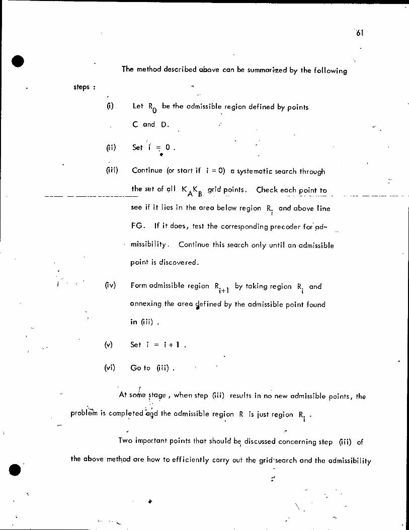
The method described above can be summori'7.ed by the following
steps "
(1) let RO be the admissible regi-on defined by points
C and D.
(Ii) Set fi' - 0 . of
(1 ri) Continue (or start if i = 0) a ~ystematic search through
~ ____________ ~the se~o~ ÇJI~ __ ~Â~IL_grid~~ints-'--~~:c~ eac~ _~?i_~~_!~
--k •
see if it lies in the area below region R. and above line 1
FG. If it does, test the corresponding precoder for'pd-
missibility. Continue this search only until an admissible
point is discovered.
\Iv) Form admissible region R. l by taking region R. and 1+ 1
annexing the area iefined by the admissible point found
in (Iii)
(v) Set i = i + 1
(vi) Go to \1 ii) .
'At so~e stage, when step (Iii) results in no new admissible points, the \ ,
'\ . "
probleÎn is compl~ted~d the admissible regi.on R is just region Ri
Two important points that should b~ discussed concerning step (Iii) of
the above method are how to efficiently carry out the grid'search and the admissibility
\ \
-,

62
" tests. Rather than searchi'l1g through the set of ail 'grid points in a random order, it
should be more efficie';t to search in some organized manner. One promising id~a
is to search through the grid points in the order of increasing n + n X y
This causes
points which are on the average farthest below the region R. to be tested first. This 1
method seems to be ~ery efficient because when an admissible point is discovered, it
defines a comparatively large area to be annexed to region R.. This not only causes 1
\ .-----.. region R. 1 to be a much better approti'mation to the entire admissible region R but
1+
if also greatly reduceJj _the number of grid points ~ying in the area between R. 1 dnd 1+
line FG) which remain to be tested.
, ' Experience has shown that cbreful ordering of a large ~umber of grid
points according to n + n is usually not practical but luckily a rough ordering of x y
this nature is already available From the results of Steps A and B. During the method
followed for these two steps 1 the precoders were arranged accor~ing to the number of
groupings of two or more source letters. But, on the average, precoclers ha~ing the
larger number of such groupings tend to have the smallèr entropies. Therefore, a prClc-
tical method of performing the grid search ca,n begin by searching through the precoders
whose X and" y mappin9 schemes have the maximum numbers of groupings of two or
more source leaers. The search then continues l by considering precoders which have
diminishing numbers of source letter groupings.
An imp~rtant operation which must be performed d,uring the grid search
.' is the testing of various. precoder schemes for admissibi lit y • Acçording to Theorem
'3-1, one admissibility testing procedure is to form the l1latrix P correspondi,ng to the , ,
f
1
1
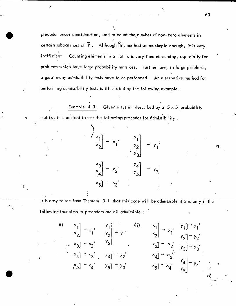
!., - 63
precooer under consideration, and to count the,number of non-zero elements in
certain subr;natrices of P. Although fhis method seems simple enough, it is very
inefficient. Counting elements in a matrix is very time cbnsuming, especially for
problems which have large probability matrices. Furthermore, in large problems,
a gteat many admissibility tests' have to be performed. An alternative method for
performing ad~issÎ~i 1 ity tests Îs i Ilustrated by the following example.
Example 4-3; Given a system described by a S x S probability
l' ~ •
" matrix, it is desired to test th: following precoder for àdmissibility :
X 1
1
X 1
2
1
, J t It Îs easy to see from Theorem--~":-lthatthtscocfeWTITbea(rmissible if and only if the
1
following four simpler precoders are 011 Q'dmissible
(1) x] ] y] ]
(1 i) X]] ~ Yl] ... y 1
-<Xl Xl 1 1 x2 l YL -; Yl x2 l
Y2] -> Y21
x3] ;zt x2' Y3 x
3] .... Xl -'
2 Y3] ... '131
x4] ... 1
Y4] .... 1 x4] .... -x/y x3, Y2 3
:S] .... x ' YS]
.... • 1 X ] .... X 1 Y4]~Y4'
4 Y3 5 4 YS -.~ . ,,~
~
\ •• -.r':
~ \ ..
,""
e
"
.'
64
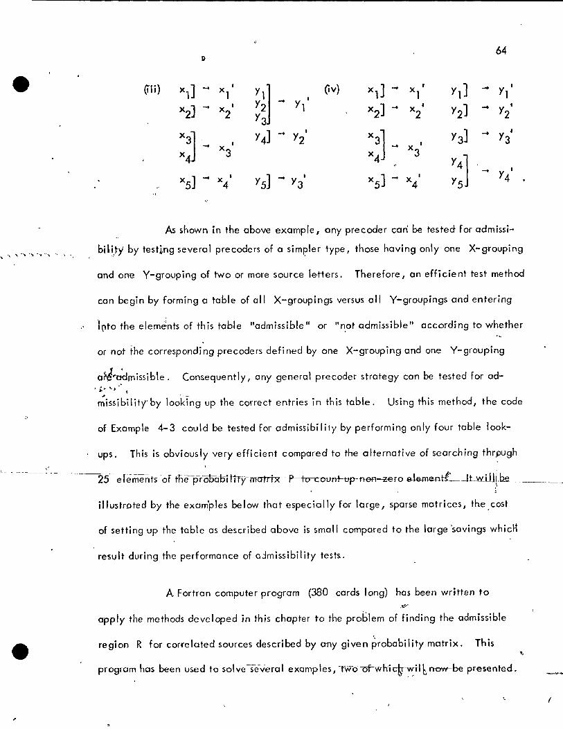
(Iii) xl] .... x ' y 1] (iv) xd .... 1
Yl] - Yl' 1 xl Y2
... Y l' x2] .... x 1 x2] ... 1
Y2] ... Y ,
2 Y3 x2 2
X 3] Y4] ...
1
Y3] ... Y3' .... 1 Y2 X 3] ,
x3
... x3 x4 x4
Y41 .... Y , xS]
.... x ' YS] .... 1
xS] .... 1
4 Y3 x4 YS 4 . '1
As shown in the above example, any precoder can' be tested for admissi
bil~ty by testlng several precoders of a simpler type, those having only one X-grouping
and one Y-grouping of two or more source le,Mers. Therefore, an efficient test method
con begin by forming a table of 011 X-groupings versus 011 Y-groupings and entering
lrto the elem~nts of this table "admissible" or "n,ot admissible" according to whether
\
or not the corresponding precoders defined by one X-grouping and one Y-grouping
arlrodrnissible. Consequently, orly general precoder strategy can be tested for ad-.;. .. \,)"""
~issibilittby 1001<1ng up the correct entries in this table. Using this method, the code
of Example 4-3 could be tested for admissibilily by performing only four table look-
ups. This is obviously very efficient compared to the alternative of searching thrpugh
L_ - --- - -~----25-erements -of tne-probat5îtîTy matrix P 10 count--1Jp---fteA.q€Ho-e-lementL--1Lw.ill(.~ ____ ~ __ -' ,
illustroted by the exam'ples below that especially for large, sparse matrices, the,cost
of setting up the table as described above is small compared to the large 'savings whicK
result during the performance of aJmissibility tests..
A Fortran computer program (380 cards long) has been written to -~
apply the methods developed in this chapter to the problem of finding the admissible
region R for correlated sources described by ony given probability matrix. This
program has been used to solve -sev-eral examples, Twoot--wtrh:tr~know-be presented. -..... ....,..
{
65 ~
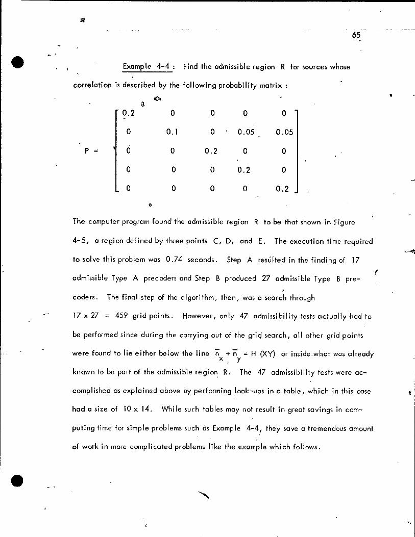
Example 4-4: Find the admissible region R for sources whose
correlation is described by the following probability matrix :
ô a 0.2 0 0 0 0
0 0.1 0 0.05 0.05
P = 0 0 0.2 0 0
0 0 0 0.2 0
0 0 0 0 0.2
u
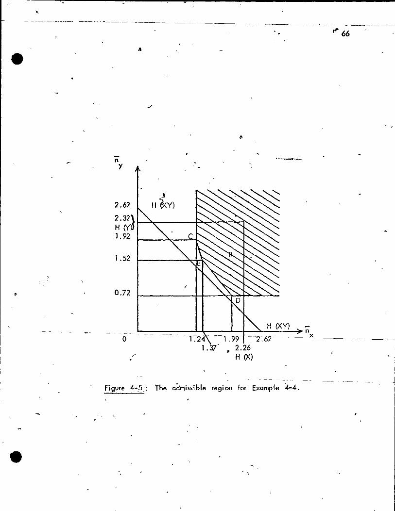
The computer program found the admissible region R to be that shown in Figure
4-5, a region defined by three points C, Dl and E. The execution time required
to solve this problem was 0.74 seconds. Step A resûlted in the finding of 17
admissible Type A precoclers and Step B produced 27 admissible Type B pre-
coders. The final step of the algorithm, then, was a search through
17 x 27 = 459 grid points. However,only 47 admissibility tests actually-had to
be performed since during the carrying out of the griq search, ail other grid points
were found to lie either below the line ri + ri :; H (XY) or imide-what was already x. y
known to be part of the admissible region, R. The 47 admissibility tests were ac-
complished as explained above by performing ,Iook-ups in a table, which in this case
had a size of 10 x 14. While surh tables may not result in great savings in com-
puting time for simple problems such às Example 4-4, they save a tremendous amount
of work in more complicated problems like the eXÇlmple which follows.
,.
: 1 \
~
-
n y
2.62
2. 32l H (Y) 1. 92
1.52
0.72
o
::
-_.- ----~----
fit 66
~" ....... -.,-.... )
H ~y)
H (XV) -----------~~----~_*--~--~~~n
---T.or- x
, 2.26 H (X)
~-~----------- ~-~--
Figure 4-.5.: The adnissible region for Example 4-4 . ..
is
P
-,
1 1 ,
67
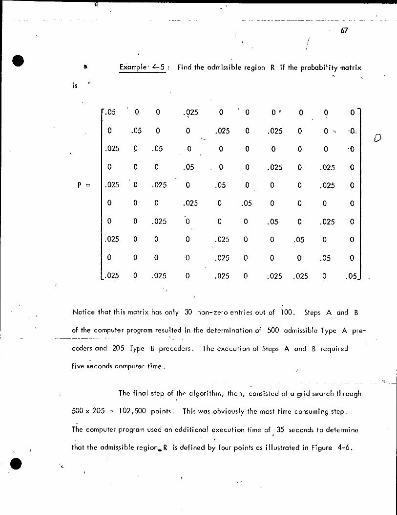
• Example' 4-5: Find the admissible region R if the probability matrix
.05 0 0 .025 0 0 o li 0 0 0 ,
0 .05 0 0 .025 0 .025 0 o " ,(1,
.025 P .05 0 0 0 0 0 0 -0
0 0 0 .05 0 0 .025 0 .025 -0
= ,025 0 .025 0 .05 0 0 0 .025 0
0 0 0 .025 0 .05 0 0 0 0
0 0 .025 0 0 0 .05 0 .025 0
.025 0 '0 0 .025 0 0 .05 0 0
0 0 0 0 .025 0 0 0 .05 0
.025 0 .025 0 .025 0 .025 .025 0 .05
Notice that this matrix has only 30 non-zero entries out of 100. Steps A and B
of the computer program resulted in the determination .of 500 admissible Type A pre-
coders and 205 Type B precoders. The execution of Steps A and B required
five seconds computer time .
The final step of thf' algorithm, then, consisted of a grid search through
500 x 205 :::: 102,500 points. This was obviously the most time consuming step.
-The computer program used an additi onal execution time of 35 seconds to determine
that the admis,sible region. R is defined by four points as illustrated in Figure 4-6.
0
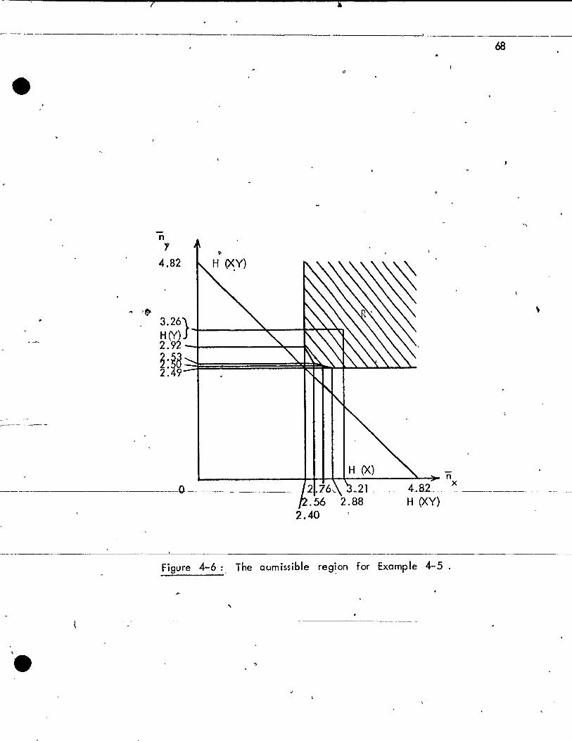
l'
-- ------------------_._--
-~--.------
---------------_.
68
n ., 4.82
~ __ ----------~~~--------~~ n x --0 ________ ---J--...q4~r___>_L..LL----4~.~8~2--------H (XY)
Figure 4-6: The aomissible regi,on for Example 4-5 .
,

~'
69
1
The computer solution of this problem used a total storage area of 74,1"00
bytes.
If is interesting to note that out of the 102,500 grid points, far less
thon 10,000 admissibility tests nad to be performed. These tests were carried out
by referring to a table of 34 x 18 (612 e lements). The great saving in computing 1 l'
tirile due to this table i~ ôbvious when orte reolizes that a precoder scheme such as
.X I ] .... x 1 YI] 1 1 --t
YI
X3 ] .... x 1 1 Y9 2 •• >
'"
X4r x 1 Y2] 3 1 Xs Y3
.... Y2
" Y6
:;] - x 1 Y4 ] .... Y 1
4 3
.... 1
Y5 ] Y4
xe ]_ x 1
S Y7 ] 1 x9 .... Y5
- - - --~-- ----- Ys ------
x2 J x10
.... x6 •
Y 10] -- Y61
- ~- - --- - - -- - - - ---- ~----
could be tested for admissibil ity by looki~g up just 12 entrles in the table instead
of the old way of partitioning matrix P and sorting through 100 entries to count the
Furthermore, the saving is magniFied due to the fact that thousands
of tests had to be done.
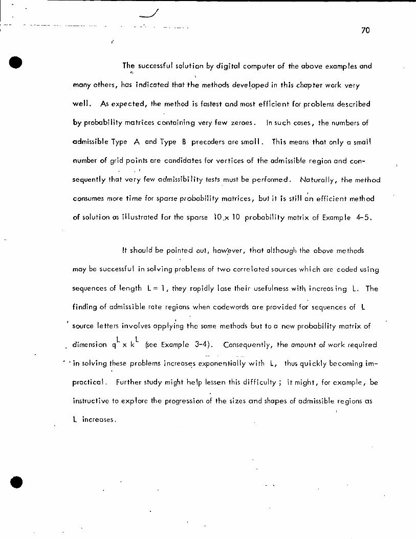
-- ~ -- -70
The successful solution by digital computer of the aboye exemplés and <.
many others, has indicated that the methods deve!.oped in this chapter work very
weil. As expected, the method is fastest and most efflcient for problems described
by probabilÎty matrices containing very few zeroes. In such cases, the numbers of
admissible Type A and Type B precoders are small. This means that only a small
number of grid points are candidates for vertices of the admissible region and con-, f
sequently that very few admissibi lit y tests .must be performed. Naturally 1 the method
. consumes more time for sparse probability matrices, but it is still an efficient method
of solution as illustrated for the sparse 10,x 10 probability motrix of Exomple 4-5.
It should be pointed out 1 how:ever, that olthough the above methods
may be successful in solving problems of two correlated sources which are coded using
sequences of length L = 1, they rapidly lose their usefulness with increos ing L. The
finding of admissi ble rate regions when codewords are proyided for sequences of L
J source letters inyolves applyi'ng the some methods but to a new probability matrix of
dimension qL x kL
(see Example 3-4). Consequently, the amount of work required
• 'in solving these problems increas~s exponent.ially with L, th us quickly becoming im-
practical. Further study might help lessen this difficulty; it might, for example 1 be
instructive to exp lore the progression of the sizes and shapes of admissible regions as
l increases.

71
) 1 CHAPTER' V
ALTERNATIVE CONFIGURATIONS IN CORRELATED SOURCE CODING
ln this chapter, the theory of variable rength coding will be extended
to apply to ail of the sixteen different coding configurations introduced in Chapter 1
(see Figure 1-4). It will be assumed here Gust as in Chapters III and IV) that the
encoders are constructed in two stages as illustrated in Figure 5-1. However, in order
" to ~eal with some of the new coding arrangements, it is neces~ary to generalize our
definitions for the precoders. Consi'der, for example, the p~oblem depi cted in
Figure 5-2, where a single pre coder has khp~~e-'dge of the outputs from two sources
X and y. We must redefine this precoder as being a transformation from the set of
011 (XY) outcomes xl Y1 ' x2 Y1 ' .. ,xk Yl ' xl Y2 ' ... "~', and x k y , to a li q
new set of letters zl ' , z2' , ... , zN'. This definition can be further extended to
allow coding for sequences of l (XY) outcomes.
It is revealing to determine for the system of Figure 5-2 what minimum
,,. sequence from, for example, source Y with zero probability of error. Since Theorem
2-3 is not strong enough to handle this situation, a more general theorem will now be
proven. l '
Theorem 5-1 : For the system of Figure 5-2, the decoder can reconstruct ,
the output sequence from source ':( with zero probability of error Wand only if
fi ~H(Y). y ,
" -
•
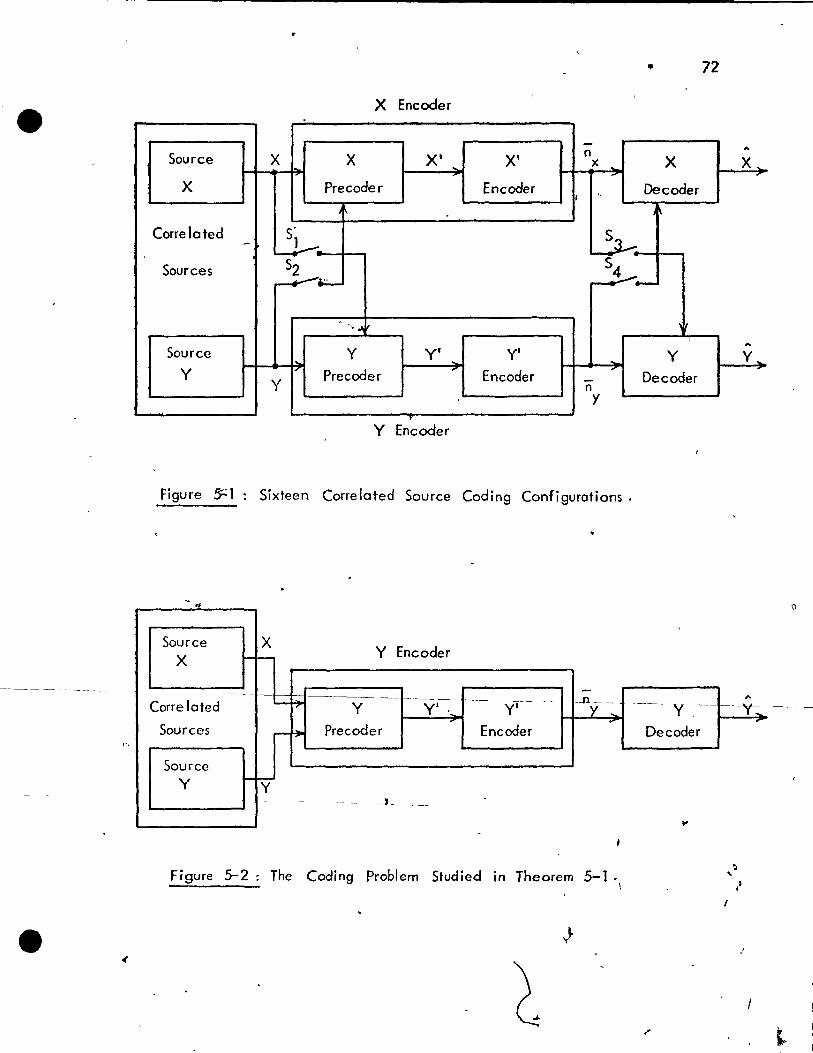
• 72
X Encoder
- .. Source X X X' X' n
X X x ~
~
X Precoder Encoder c Decoder , J
" J
Correlcted S' 53. - L2--. S ~ Sources $2 4
~i::-
. ''>,J
,.. Source y Y' Y' Y Y ,
Y Precoder 7'
Encoder .,.
Decoder y -n y
y Encoder
Figure ~1 Sixteen Correlcted Source Coding Configurations.
.,
Source X Y Encoder X 1- -
----c---- - -------- -Dy __ ,..
Corre \cted - ~ y Y' " y' - - ----- y --- I-----y-:...
.,. Sources r-~ Precoder Encoder Decoder
Source Y 1-~
- - ---L --
\0'
Figure 5-2: The Coding Problem Studied in Theorem 5-1. \
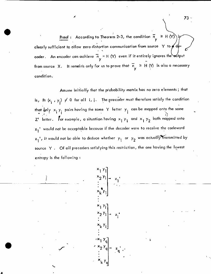
73 ".
/
Proof: According to Theorem 2-3, the condi tion n y
cleorly sufficient to allow zero dis'~ortion communication Ftom source
coder. An encoder con achieve n = H (Y) even if it entirely ignores the y ~
From source X. It rell'1(liris only for us to prove that n :2: H (Y) is also a necessary y
condition.
Assume initially that the pr'obability matrix has no zero elements; that
is, Pr (x. , y.) -1 0 for ail i, i. ~he prec;der must therefore satisfy the condition 1 1 .
that ~nly x. y. pairs having the sarne Y leffer y. • .; .' 1 l ,1
Z' letter. ror example 1 a situation having xl y 1
con be mapped onto the same '\ -, If
and x 1 y 2 both mapped onto
Zl' would not be accept~ble because if the decoder were to receive t~e codeword
zl" it would not be able to deduce whether Yl or Y2 was actualf);~f~nsmitted by
source Y. Of 011 precoders satisfying this restriction, the one having the lowest .>

This scheme has an entropy of " q k k \' \' ,..-,
H (Z') - , - L [ L Pr (x., y.) ] 1092 [L 1 1
j=l "i=l i=l
= q \' - L Pr (Yi) 1092 Pr (Yi) = H (Y) .
j=l
.. -
74
Pr (x. 1 y.) ] ' 1 1
, ;
Therefore, according to Theorem 2-3, tb~ decoder of Eig~e 5-2 con only reconstruct
the output of source y with zero probability of e~ror if fhe average codeword length
- ----~ -- -satisfies Tl ~ H (Y). This conclusion is still valid for the case when zeroes ore y
allowed"in the probabi lit y matrix because if ony outcome (X. 1 y.) oc~urs with pra-l J
r
bability zero, the precoder moy map x. y. onto any one of the z'~letters without 1 1
changing the probability of error. Moreover, the entropy colculotion is unaffected
since Pr (x. , y.) 1092 Pr (X. , y.) = 0 . 1 1 1 1
The above result olso holds for the situation where the precoder is
allowed to he a mapping for sequences of (XY) outcomes. This con be shown...easily .
1>ypretelldillg the-t-the~fette.rs- -X..r~.t-!...-'m.L><i< L.9_nd_ )'1' -Y2 1 ... 1_~ct-__ actua_~I~
represent sequences of L letters from simpler sources. ,
,)
Let us first consider the four correlated source coding configurations in
Figure 5-3, 011 of which are characterized by uncoupled decoders. For Case 1,
sources X and Y ore encoded and decoded iRdependently and therefore the results
of Chapter Il for single sourceS con be opplied. That is, the source outputs for Case
1 con be communicated to the decoders with zero distortion if and only if n ~ H (X) x
and ri ~ HM. y . ,
.'

75
~I 1
n
~I ,..
Source X X x f 'X X
X Encod,er Decoder >0
1 Source Y Y n
> l, y J y
l Y Encoder Decoder >-
Case 1
~ .. , - ,..
Source _ X - X n
X X ... x ....
X
\ Encoder
".
Decoder .,.
1
- ,..
Source Y y n y y y y ,
Encoder ,..
Decoder ... , -' )"
Case 2
n ,.. c
Source X X X X X, _ ... ,
X ,..
Encoder Decoder ,..
1 ny ,.
Source Y Y .... Y y .. ,. Y Encoder Decoder
Case 3
- ,.. Source X X
n X X .... ... x ...
X
X Encoder
,.. Decoder ".
- ,.. Squrc~:':" y y n y y .... y ....
y .. Encoder
... Decoder
.. r.
Case 4
figure 5-3: Correlated Source Coding with Uncoupled Decoders .
. -"

_ . ..
r '
76
1 Cases 2, 3, and 4 appear to be slightly' more complicqted but by
applying Theorems 5-1 and 2-3 to thes'e problems, it is easy to see that the ad-
missible regions are ail idéntical to that for Case 1, namely the area n ~ H (X) , x
n ~ H (Y). I~ should be emphasized that these results hold even w~en coding is y
permitted for seque nces of source letters.
Consider next the four correlated source.coding arrangements illustrated
in Figure 5-4, those characterized by completely coupled decoders. Of these four
problems, Case 8 has the simplest solution. Since both of its encoders are allowed
to see the outputs From both sources X and Y, the entire source o,utput information
.. can be communicated to the decoder through e ither one of the encoders exclusively.
Thus, (H (XY), 0) and (0, H (XY)) are admissible rate points.and C!.ccording to ,..
Theorems 3-2, 3-3, and 3-4, the admissible rpgion R for Case 8 must be the
are~' ri + ri ~ H (X Y) . ,? X Y
Unfortunate Iy 1 ii is not possible to derive any such simp te formula to
describe the admissible region for Case 5. This fact has already been demonstrated
very clearly, Case 5 being none otper thon the problem studied in such detail in
Chapters III and IV. However 1 with the aid of t~e following theorem, it yv-ill be 1
shown that the admissible region for Case 6 takes a very simple form. \
Notè Htat
Case 7. does not need to be st,udied separately because it is just a symmetric version
; df Case 6, formed by interchanging the roles ·of X and Y •

'1
Source
X - --
Source
y
Source
X
Source
Y
~,
, Source
X
'\
"Source
y
Source
X ~
,
Soyrce
-- .... ---~
Figure 5-4 : Q
e ..
l -- ------
X -
y -.
,X
y G-
'X " --,< '" l, .
Y
li
"
~ X Encoder
y
Encoder
Case 5
X Encoder
Y
Encoder
Case 6
X Encoder
Y
Encoder
Case 7
X Encoder
y
Encoder
Case. 8 t
'.
/
• 1 )
-nx .. X
oyX Decoder
y ... Decoder
,)
--.;-- -- ~---- -
n
-n x ..
nyX 4 ...
~J ..;
X Decoder
Y
Decoder
X Decoder
Y
Decoder
X Decoder
y
Decoder
--
-
....... -"" .....
Cor.related Source Codingot with Coupled Decoders.
<'
l
:, ._-~------ -- -.-- .... ____ ~ _ ____ L.
77
'" X
-'J'
,
'" 0
y "
A
X o
L...
A
X .-
" Y , ,.
t "
~
•
t .,.'

the point
o
Theorem 5-2: (see Lu [3J) For the system illustrated in Figure 5-5,
(n ,n) == (H (X), H fY 1 X)) is an admissible rate point, where x y
H t't, 1 X) is called the conditional entropy of y given X and is defin~ by
C"J
H t't 1 X) Â
k q
- L l i= 1 j= 1
Pr (x. 1
/ Proof: Since the output of source X is always kno~n to the Y pre-
cod~~, -it is' p~ssible to design a y precoder which employs several differ.ent coding
strategies depending on what outcome is produced by source X; Consider, for ex-
ample, a y precoder wh)ch operates in the following manner: when the output of
source X IS xi ' the Y source !etters are Huffman coded according to the set of
and Pr (y 1 X')"l q 1 By definin~
ny 1 xl' ny 1 x2
' ..• , 'and ny 1 xk
to be the average codeword lengths corres
ponding to these k different Y-codes, the overall average codeword length n can y
be expressed as follows
k
n y = l Pr (xi)
~7~-
n y 1 x.
1
Note tl~at it, woold be possible for the above y encoder to transmit the output
sequence from sQurcc y' to the 'r decoder with no errors i~nTy-the y âecode" -
>--------,.---,o..rlh-s.,..o4.had kllowledge,of tl:w X output HH~!lenCe 4:>ecause "knowing X wou Id enable ~
the' decoder to deduce which of the ~ coding ';chemes was actuall~ used by the y
precoder) . Dfst9rtionless commu'nication con therdore be guarànteéd by choo?ing . i
\ 1
the X precoder to be uniquely d~codable (which it must be in, any case) ..
---r~

, ,
..
e· ..
._-~-----
"
-1..
Source X ~ X XI .. n
XI X .. X ",
, ,. Preceder ~ Encoder
, .
Correlated
Sources .
'So~rce Y':- - ~ y yi yi ny ... ......
y ...
Precoder ...
Encoder ,.,
0
,~
Figure 5-5: The source coding sySotem studied in Theorem 5-2 . •
...
D'
c
..
79
,..
X X - ..
Decoder' '-
,.. y y
Decoder .,.
-Cl
.,...
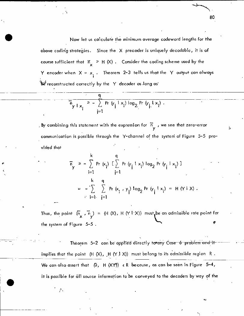
.,-----~~--1 -- -- - - ~-- --
BO
Now let us calculate !h~ minimum average codeword lengths for the
above codin"g strategies. Since the X precoder is unique Iy decodable, it is of
course sufficient that il ~ H (X). Consider the coding scheme used by the x
y encoder when X = X. 1
Theorem 2-3 te Ils us that the Y output can always
1sJ reconstructed correctly by the Y decoder as ,long as'
q
l Pr (y. 1 x.) 10g2. Pr (y. lx.) . 1 l , 1- 1
n ~ y 1 x.
1 j= 1
_ By combining this statement with the expressi on for iï ,we see that zero-error y
communication is possible through the Y-channel of the system of Figure 5-5 pro-
vided that
n y
k q
= - 'I I u' i=l· j=l
q
(\ Pr (y. 1 x.) 1092 Pr (y. 1 x.) ] L 1 1 1 1-
j= 1
Pr (x. , y.) 1092 Pr (y. 1 x.) = H fy 1 X) . 1 1 1 1
Thu" the. po; nt (ri x ' n yl = (H (Xl, H (Y 1· X)) must tan adm ;ss; bl. rate po; nt :0' the system of Figure 5-5.
, \
,
i>
Theon~-m- 5-2 -can bè- dpptîeâ -dîrectty to-anTfue--6--prOhFe-rITund--it----~
implies that the point (H (X), ,H fy.l X)) must belong to its ~dmissible region R.
We can also assert that (0, H (XYj) E R because, as can be seen in Figure 5-4,
it is possible for âll source informa,tion to'be conveyed to the decoders by way <;>f the
'-

1
'-
81
y channel alone. Since the points (H (X), H (YI X») and (0, H (XY)) both lie
on the line n + ri = H (XY), Theorem 3-4 t'e Ils us that the e.ntire admissible : x y
region R fol' any Case 6 system is si~p~y that shawn in Figure 5-6. Observe that
no points below the hori1U)ntal ~ine-ny = H (Y 1 X) can belong ta R because even
if n is increased above the value H (X), the X encoder can be no better than x
uniquely decodable and consequently no further improyements can be made_tQth~e----'YI--____ _
encoder.
,. Even though the admi~sible region for Case (> has now been discovered,
it is still useful to mention how one might go about determining the set of admissible
precodets (this problem will arise in connectidn with Case 10). A careful inspection
of the Case 6 system reveals that it can be redrawn as in Figure 5-7 sa as ta make , . , ,
if oppear very similar to a Casé 5 prot:rfem, the 'most'notable difference being that
source Y has been replaced by the joint source XY. By relabe ling source XY as
a new source Z and 'by realizing that the decoder of Figure 5-7 can be thought of
as producin"g estimates X and Z rather than X and, Y (these two situations are
equivalel'lt because X and Z (X, Y) can b~ recovered with -zero probability of error
by d decoder if and only if X and Y can) 1 it follows that the system of Figure 5-7
is mathematically identical to a Case 5 problem for t';"o correlated sources X and
- - - - ---- ,
Z. Therefore, by setting up a new probabil ity , to describe the corre-
lotion between sources X and XY instead of between Sources X and y, the r~thods ------- - -- - -', -~
- - !, ~ ~ ~ -- - - - - - -- - --- -of Chapters III ond IV can be applied .directly 't>o find the admissible precoders for
any Case 6 problem. (
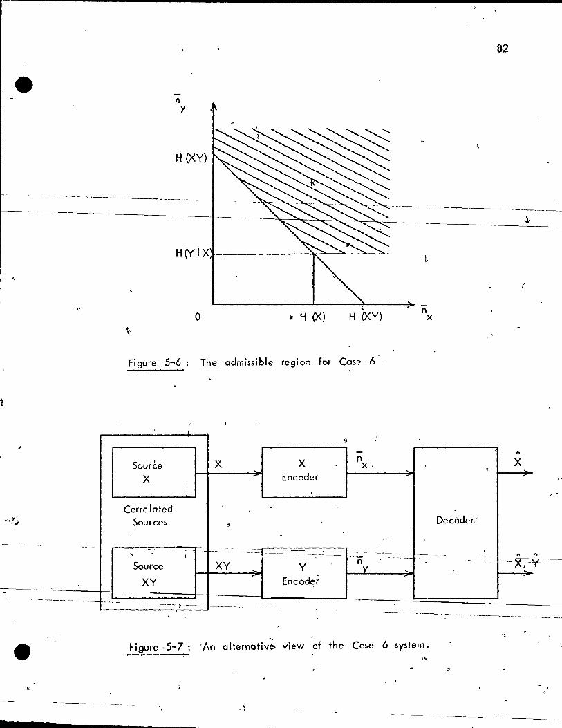
• 2
n y
H (XY)
---------
\
o " H (X) H (XY)
Figure 5-6: The admissible region for Case -6'.
Sourée
x
Corre lated Sources
J
J
x X Encoder
n x·
n x
Decôder!
82
----"--. - -------
Figure.5-7: 'An alternotiv~~ view of the Ccse 6 system . . .,.
x
, ,
....
~ 83
Consider now the four systems depicteq in Figure 5-8. These cases
are characterized by a Y de coder which opera tes without knowledge of the X en-
coded message streaf even though the X decoder has access to both codeword
\
sequences. While it is not trivjal to determine the admissible regions f9r Cases 9
and la, very simple regions existfor Cases 'l1,a~d 12. For Case 11, it follows - - -- - , ~ - -~ - - ~
directl" From Theorem 5-2· {by inte,--,rc=h-,-"a,"-,-n~i-,-,n~~X-,--a:::::n,-"d~--'Y-'-~~-1'~~~'-LJ.~~~).L) _____ ---J
is an admissible point. Since this point lies on the line 'fi' + n :::: H (X Y) and x y
since the' Y encoder for Case 11 must be unique Iy decod~ble, the admissible region
R is just the rectangular area sh6wn in Figure 5-9 .
. ~ Theorem 5-2 con also be applied to Case ',12 to show that (H (X 1 Y),
H (Y)) ER. Since ail source information for Case 12 can be transmitted to the
- . decoders through the Y channel alone, if can also·be stated that (0, H (XY)) E R
1\ By'realizing that these two points lie on the line n + n = H (XY) and that
x y
Thec;>rem 5-1 requires that 'fi'y ~ H (Y), the ent~re admissible region R for Case
12 is found to be that drawn in Figure 5 ... 10.
, ln order to solve the Ca~e 9 problem, it is necessary to' make use of
some of the results of Chapters III and IV. This is a logical approach because
--=-==--=::--:-_- there turns out to be a close re latiunship between the Case._ 9 and Case 5 con-- - \ - --
figurations. In fa ct , it is easy to recognize thot any precoder scheme which is ad-
_~ i ss ib_l_e _f_or __ Ças_e _~ __ r:n.~~t ~ 1 ~ '? be a dm'!i s::-::s:Oi Lb '-1 e:-Tf o::r-::--<_Ci"""_ a=--=:-:~:-_-5-'::-.~-_LH~0::-:. w-:-:-::-e:-:"ve::::-r=-,--=-s ~1O~c=-=():--rIfh""e=--''''y'~'-----------,--- . -- -
encoder for Case 9 must always be unique Iy deèodable, ,the set of 011 admissible
-----._~,----------- .

"
Source X ... X
, ,
, . Source Y ... ...
y ,
-Source )(
X \ ~
Source Y .... '" y
Source X .. 'X .<jIj
Source Y 1 , , Y
Source X
X
Source y
y
X Encoder
Y
Encoder
Case 9
-.
X --Encoder
~
y
Encoder
Case 10
X
Enc(,der
y
Encoder
Case 11
x Encoder
y EnCOder'·-
Case 12
-n
x ....
j -ny
--_. - . _. ----nx
l-
-n Y
-nx
-ny
n x
\
'j
11
~
X Dec;oder
y
Decoder
-
X
Decoder
'Y Decoder
..l'X
Decoder
y
Decoder
.- X
Decoder
y
_______ u __ --tTgure -5=8: Corre lafed Source C6è1îng w.fn Partially Coupled Decoders.
1
~
84
ft
X~ -~
\ '
•
ft
y .. o
- ---,.-
X
'-'
" Y .,
" X -"
1
" y>
..
y
'.
---_._-----_.---- ---- --- .-----

,
· '
n y
H (XY)
H (Y)
H(Y 1 X) c
, , ;.:~
o H(XI~ H (X) H "(XY)
Figure 5-9: The admissible region for Case 11
11 Y
H (XY)
o ,
..
H (X} H (XY) 1
Figure 5-10: The, admissible region for Case 12.
85
-n x
l' .
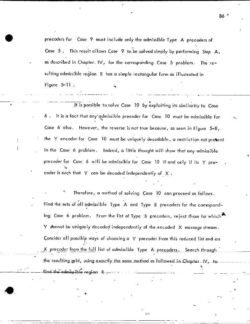
86 •
precoders for Case 9 must include only the admissible Type A precoders of
"
Case 5. This result allows Case 9 to be solved simply by performing Step A,
as described in Chapter. IV 1 for the corresponding Case 5 problem. Thè re-
sulting admissible region R has a simple rectangular form as itlustrated in
Figure 5-11 .
------------- ------- -- \- '
.It is possible to solve Case 10 by exploiting its similarity to Case
6. It is a fact that any' a..?missible precoder for Case 10 must be admissibl~ for ....
Case 6 0150. However, the reverse is not true because, as seen in Figure 5-8,
the y encoder for Case 10 must be unique Iy decodable, a restri ction not pre'ent
in the Case 6 problem. Indeed 1 0 1 ittle thought wi Il show that aoy admissible
precoder for Case 6 will be admrssible for Case 10 if and only if its Y pre-
coder is su ch that Y con he decoded independently of X .
Therefore, a method of solving Case 10 con proceed os follows .
• Find the sets of 011 admissible Type A and Type B precoders for the correspond-
ing Case 6 problem. FrorT' the list of Type B precoders , reject those for which"
y dIonnot be u-niqüe Iy decode~ independently of the encoded X message stream.
Consider 011 possiblr ways of choosing a y 'pr-ecoder from this reduced list and on Il.
x -.erecoder from...!b~J.~U ist of admissible Type A- precoders. Search through -----~ -->,
.... ______ Jh~ IEt~ulting--9rid, using .exactly_lhe~ameJùetbod as foliowedJn Chapter - LV,.- -!o- ________ ~,
;J.
--~-----~Ie-f-egion R
')
. ~
~.
--------------------------~====================~~==~=======-=-==~~--~-----~-----~

e··
.,.
.c.,
t
n y
H (XY)
H (Y)
.. .'
"J ~I
H (Y 1 X) I---+----+-~
o H(X 1 Y) H (X)
Q
n x
, "
-Figure ~-11 : The admissible region for Case 9 .
/
".,.-------~-t-=:::-::=--=-=-=-==--=====~-----===. ~ --"
87
1 1
i /
(

1
...
The only remaining correlated source coding configurations to be '.
- n
, " ~onsidered are the four c~ses i\l\Jstr~ted in Figure 5-12. ~
Cases 13, 14, 15, and
16 correspond exactly to CaseS 9, 11, 10, and 12 respecti~e Iy except that
the roles of . X and Y have been reversed. Consequently, the problems of
Figure 5-12 can be solved using the methods developed above.
, ,
"
, "
.. .
88
------~-<~------
...
v

,
y - •
-n Source 'x -x , x « , X - --
~
'\ -- -
X Encoder Decoder
-Source V ... Y ny ... y
y ".
Encoder ,
Decoder , . Case 13
-n Source )( ... X x .. X
X
'\ Encoder
'\ Décoder
-n Source Y .. Y Y
~ Y -" '" y Encoder Decoder
Case 14
. n
X Source X x ... X X
--.-Encoder '\ Decoder
1 .' '1
.; . . - 1 ,
... n Source Y y Y ..... Y
Y ~
Encoder ...
Decoder' ?
Casé' 15
,/
, n Source X .. X x ... X
X
X Encoder
'\ Decoder
.
-Source Y
-- - - n --y y -
v .. y ;'
\ Encoder ,- , Decodef
-' ---~---~--- --------Case 16
,-._--, 1 j 1
Figure 5-12: Corre lated So'urce t~ing with Partially Coupl,ed Decoders.
.. ;
89
" X
- - --
y ~
,. X .. ,
,. y ...
" X, ,.
,.
y .... ,..
,..
X ..
A.
y ... "..
)

-e
,1'~ i
1
, / ,
1
90
CHAPTER VI
CONCLUSION
• ln summary, the principal achievement of this thesis ~as been the
presentation of a compact theory regarding variabl~ length coding for two
correlated information sources. Methods have been successfully derived for the
purpose of determining admissible rate regions for correlated sources which are
, encoded in a.ny one of sixteen possible configurations. For simplicity, most of the ~
results in preceding chapters were ~stabtished by assuming that the precol-rs could
only provide codewords for individual source letters. But in Example 3-4, it was
.' shown how this situation can be easily ge~eralized to include coding for seq~ences
of l source letters. Actually, this approach in correl~ted source coding is
1-
analagous to that used in Huffman cocHng for single source.s, because in both cases
the finding of optimum codes depends upon an initi~1 assumption as to the ,iet'lgth of
sequences of source lett~rs to be encoded. -in fact, the major contribution of this ~
thesis may be considered to be the generalization of the Huffman code to more com-"
plicated source structur~s.
Naw that the theory of joint coding for h';o sources has been
fhofough!'f.-tnvenigated'I it is-quitenoturol -ta ÎnquÎ(e Îf the resutts of this"thesi~ con , 1
, , ,
bELe)~,t!?l]de_d_ to 'the problem of variable tength~coding for N corre lated sources
(see Cover [1 J) . ~
Ta try and answer this question, consider the arrangeme_nt of 1
three sources i1tustmted in Figure Q-l. Jyst as in Chapter Ill, ft is conventent·as
q )
'" ,- - .- ,_. --_ ..
r
1.
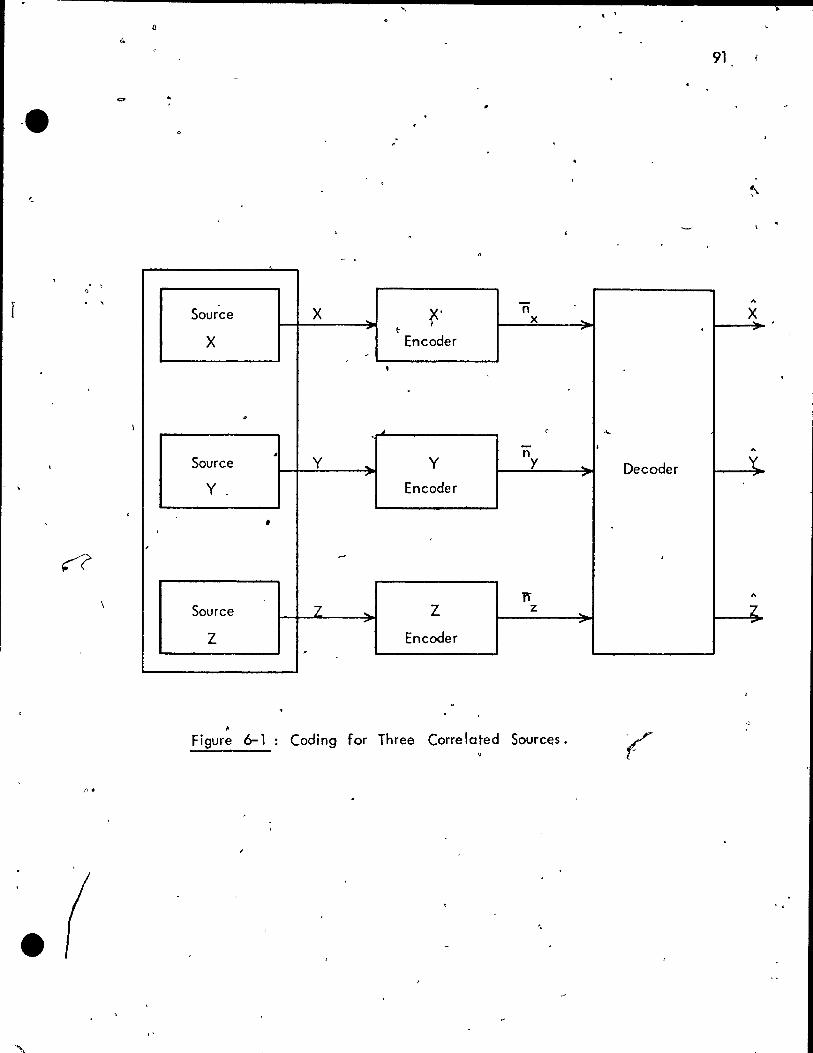
, o
91
-e
'-
. , . , ,..
Source X r n X .. x ~ , b . ..
X Encoder , .
• .
~
0 "'-
- 1 ,.. Source
1 n '( y ... y y Decoder ,. .,. '" y - Encoder
, ,
.- )
1'i ,. Source 7 ... Z z Z ,. -,. ...
Z Encoder ,
Figure 6-1 : Coding for Three Correloted Sources. -/ r
l' •

\ ;. (
\ 1 J < 92
an initial step to set up a probability matrix P to desc.ribe the correlation between
these sources. As indicoted in Figure 6-~,..,.lowever, 0 tlotree-dimensionol orroy is
needecfytostore the complete set 6f joint probabilities. Proceedî~gas in Chapter III,
" J .. 1
it is possible to prove necessary and sufficient conditions concerning the admissibility
of precoder schemes for the system of Figure 6-1. As before, the reordering of 4J
source letters defined by cny specifie precoder scheme suggests a corresponding way
of subdividing the probabilitx array of Figure 6-2 into a set of three-dimensionol () / '\
blocks. It turns out that if each su ch block contains at most one non-zero element,
then and only then will the precoder schem'e be admissible.
It can be shown that 011 the important concepts of Chapter III ..... can be .. exten'ded to apply not only to the above system cif ,three sources, but more generally
\
._ to the problem of N correlated s'curees. Unfortunately, howevar, the replacement
of matrices by higher order tensors make~ the the ory much morè difficult tO'visualize. - '
Furthermore, even if it were possible to generÇllize the solution methods of Chapter'
\ IV and compose co!",puter programs to tackle multi-sourc~ problems, the omount of
computing work required would quickly become unmonageable with an increasing
number of correlated sources. Besides this, there is even one more complication not
mentioned unti 1 now, the fact that in undertaking a complete study of the problem of
N . 1 d . . "d 22N (N-1) d'ff' f' : corre ate sources, It IS necessary to consi er 1 erent con IguratlOns
for the encoders and decoders, a seemingly hopeless proposition for N ~ 3

P ,
,
=
. Pr (xl' Yl' zl) .", ::'~:" Pr (xk ' y]; zl)
, . ,
.'
. " .
,
, "
..
Figure 6-2: A Probabil ity Array for Three Correlated Sources. d
, ,
"
\ 1 , "
, .
93
~ "
.r
•
" ,

. \
.e
• \ 1
i •
\J \
ln ,conclusion, it !s, hoped th~t this thesis has' been su~cessful in
shedding much light on the subject of variable letlgth coding for two or more \
94
correlated>sources, a problern which has been unsolved for sorne time. Nevertheless,
many questi?ns still remain unanswered and several related problems remain to be
explored.
, .
. ---
Il
---
f ~ , \
, . \
\ ,
\ \
f • ,

o
)
• 95
'el BLI OGRAPHY
[l} Cover, T. M., irA Proof of the Data Compression Theorem of Siepian
and Wolf for Ergodic Sources, fi submitted to IEEE Transactions on
Inforrro ti on Theory.
[2j Gallager, R. G., Information Theory and Reliable Communication,
l , New York: Wiley 1 1968.
-Lu, S. C., "Variable Length Source Coding Theorem for Correlated In-
formation Sources, rr submitted to IEEE Transactions on Information
Theory, -
[4J Siepian, D., and W~., "~oiseless Coding of Corr!lated Information , .
Sources," IEEE Transactions on Information Theory, Vol. IT -19,
No. 4, pp. 471-480, July 1973.
rsJ Wyner, A. D. 1 Il A Theorem on the Entropy of Certain Binary Sequences
(J
•
and Applic.ations: Pa,~t Il,'' IEEE Transactions on Information
,/ Theory, Vol. IT -19, No. 6, pp. 772-777, November 1973.
lJ
c
/
Top Related