


Languages
Pages
Legal


Validating Self-reported Turnout by Linking PublicOpinion Surveys with Administrative Records∗
Ted Enamorado† Kosuke Imai‡
First Draft: February 27, 2018This Draft: May 18, 2019
Abstract
Although it is widely known that the self-reported turnout rates obtained from public opinionsurveys tend to substantially overestimate the actual turnout rates, scholars sharply disagree on whatcauses this bias. Some blame overreporting due to social desirability, whereas others attribute it tonon-response bias and the accuracy of turnout validation. While we can validate self-reported turnoutby directly linking surveys with administrative records, most existing studies rely on proprietarymerging algorithms with little scientific transparency and report conflicting results. To shed a lighton this debate, we apply a probabilistic record linkage model, implemented via the open-sourcesoftware package fastLink, to merge two major election studies – the American National ElectionStudies and the Cooperative Congressional Election Survey – with a national voter file of over 180million records. For both studies, fastLink successfully produces validated turnout rates close tothe actual turnout rates, leading to public-use validated turnout data for the two studies. Using thesemerged data sets, we find that the bias of self-reported turnout originates primarily from overreportingrather than non-response. Our findings suggest that those who are educated and interested in politicsare more likely to overreport turnout. Finally, we show that fastLink performs as well as a proprietaryalgorithm.
∗We thank Bruce Willsie of L2, Inc. for making the national voter file available and Matt DeBell of ANES and SteffenWeiss of YouGov for technical assistance. We also thank Ben Fifield for his advice and assistance and Steve Ansolabehereand Matt DeBell for helpful comments.†Ph.D. Candidate, Department of Politics, Princeton University, Princeton NJ 08544. Email: [email protected],
URL: http://www.tedenamorado.com‡Professor of Government and of Statistics, Harvard University. 1737 Cambridge Street, Institute for Quantitative Social
Science, Cambridge MA 02138. Email: [email protected]
●
●
●
5060
7080
90
Presidential Election years
Turn
out (
%)
Actual Turnout
ANES
CCES
2000 2004 2008 2012 2016
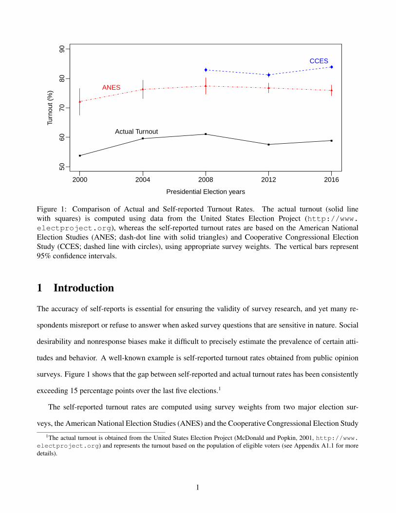
Figure 1: Comparison of Actual and Self-reported Turnout Rates. The actual turnout (solid linewith squares) is computed using data from the United States Election Project (http://www.electproject.org), whereas the self-reported turnout rates are based on the American NationalElection Studies (ANES; dash-dot line with solid triangles) and Cooperative Congressional ElectionStudy (CCES; dashed line with circles), using appropriate survey weights. The vertical bars represent95% confidence intervals.
1 Introduction
The accuracy of self-reports is essential for ensuring the validity of survey research, and yet many re-
spondents misreport or refuse to answer when asked survey questions that are sensitive in nature. Social
desirability and nonresponse biases make it difficult to precisely estimate the prevalence of certain atti-
tudes and behavior. A well-known example is self-reported turnout rates obtained from public opinion
surveys. Figure 1 shows that the gap between self-reported and actual turnout rates has been consistently
exceeding 15 percentage points over the last five elections.1
The self-reported turnout rates are computed using survey weights from two major election sur-
veys, the American National Election Studies (ANES) and the Cooperative Congressional Election Study
1The actual turnout is obtained from the United States Election Project (McDonald and Popkin, 2001, http://www.electproject.org) and represents the turnout based on the population of eligible voters (see Appendix A1.1 for moredetails).
1

(CCES). The ANES has been conducted for every presidential election since 1948, whereas the CCES
is a large-scale online survey that has been administered for every election since 2006. While the ANES
has used face-to-face interviews, it also conducted an Internet survey in the last three general elections.
The difference between actual and self-reported turnout rates is remarkably consistent during this period.
While the actual turnout rate has hovered between 50 and 60 percent, the survey estimates have always
stayed above 70 percent with the CCES exceeding 80 percent.
However, scholars sharply disagree on what causes the bias of self-reported turnout rates. Some
blame overreporting due to social desirability (e.g., Silver et al., 1986; Bernstein et al., 2001), while oth-
ers attribute the bias to non-response (e.g., Burden, 2000). Although in earlier years the ANES validated
self-reported turnout by manually checking government records, the high cost of this validation proce-
dure led to its discontinuation in the 1990s, making it difficult to resolve the controversy. Fortunately,
Congress passed the Help America Vote Act in 2002, mandating that each state develops an official voter
registration list. This enabled commercial firms to systematically collect and regularly update nationwide
voter registration files (Ansolabehere and Hersh, 2012). Both the ANES and CCES now rely on these
commercial firms to validate the self-reported turnout.
Nevertheless, the debate about the causes of the bias of self-reported turnout rates persists. Most
prominently, while Ansolabehere and Hersh (2012) use commercial validation for the 2008 CCES and
find that overreporting is the culprit of bias in self-reported turnout, Berent et al. (2011, 2016) analyze
the 2008 ANES and contend that such findings are due to the poor quality of government records and
the errors in matching survey respondents to registered voters in administrative records. In a recent
paper, Jackman and Spahn (2019) validate the self-reported turnout in the 2012 ANES by working with
a commercial firm and relying on its proprietary method. They find that overreporting is responsible
for six percentage points whereas non-response bias and inadvertent mobilization effect account for
four and three percentage points, respectively. In sum, the existing evidence is mixed as to what biases
self-reported turnout in public opinion surveys. Yet, these studies often rely on commercial validation,
making it difficult to assess why their findings disagree with one another.
2
In this paper, we contribute to this literature by examining the validity of self-reported turnout in the
2016 United States presidential election. Our validation study is based on both the ANES and CCES.
We apply the canonical model of probabilistic record linkage, originally proposed by Fellegi and Sunter
(1969) and recently improved by Enamorado et al. (2019), to match survey respondents with registered
voters in a nationwide voter file of more than 180 million records. Unlike Ansolabehere and Hersh
(2012) and Jackman and Spahn (2019) who rely on a proprietary record linkage algorithm, we use the
open-source software package fastLink (Enamorado et al., 2017) to maximize the scientific transparency.
In addition, unlike Berent et al. (2016) who evaluates the performance of deterministic record linkage
methods, we consider a probabilistic method that is more commonly used in the statistical literature (e.g.,
Winkler, 2006; Lahiri and Larsen, 2005). Our merge yielded public-use validated turnout data for the
two surveys (Enamorado et al., 2018a,b). To the best of our knowledge, this paper describes the first
effort to examine the empirical performance of a probabilistic record linkage method using large-scale
administrative records in political science.
We find that the validated turnout rate for the ANES based on fastLink closely approximates the
actual turnout rate when combined with clerical review.2 For the CCES, the probabilistic record link-
age method without clerical review yields the validated turnout rate close to the actual turnout rate. We
conjecture that because the CCES is a noisier data set with many missing and invalid address entries,
clerical review induces false negatives, lowering a validated turnout rate. For both the ANES and CCES,
we obtain similar validated turnout rates for pre-election and post-election surveys, suggesting that panel
attrition accounts little for the bias in self-reported turnout. We do find, however, that 30 to 40 percent of
the matched non-voters falsely report they voted in the election, implying that overreporting is responsi-
ble for much of the bias. This finding agrees with the conclusion of Ansolabehere and Hersh (2012) but
is inconsistent with that of Berent et al. (2016). Similar to the previous literature, we find that those who
are wealthy, partisan, highly educated and interested in politics are more likely to overreport turnout. In
addition, we find that African Americans are more likely to overreport than other racial groups. Finally,
2Clerical review refers to the process of human validation, focusing on those cases that are difficult for an automatedalgorithm to classify.
3
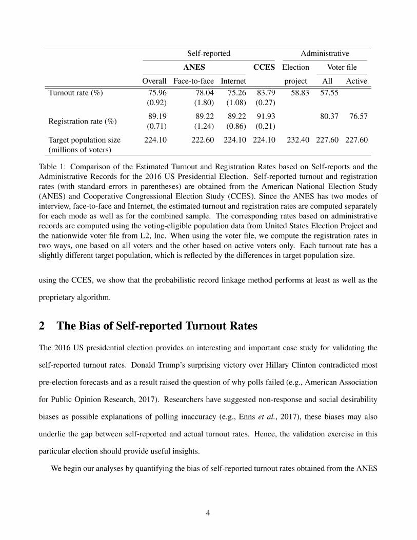
Self-reported Administrative
ANES CCES Election Voter file
Overall Face-to-face Internet project All ActiveTurnout rate (%) 75.96 78.04 75.26 83.79 58.83 57.55
(0.92) (1.80) (1.08) (0.27)
Registration rate (%)89.19 89.22 89.22 91.93 80.37 76.57(0.71) (1.24) (0.86) (0.21)
Target population size(millions of voters)
224.10 222.60 224.10 224.10 232.40 227.60 227.60
Table 1: Comparison of the Estimated Turnout and Registration Rates based on Self-reports and theAdministrative Records for the 2016 US Presidential Election. Self-reported turnout and registrationrates (with standard errors in parentheses) are obtained from the American National Election Study(ANES) and Cooperative Congressional Election Study (CCES). Since the ANES has two modes ofinterview, face-to-face and Internet, the estimated turnout and registration rates are computed separatelyfor each mode as well as for the combined sample. The corresponding rates based on administrativerecords are computed using the voting-eligible population data from United States Election Project andthe nationwide voter file from L2, Inc. When using the voter file, we compute the registration rates intwo ways, one based on all voters and the other based on active voters only. Each turnout rate has aslightly different target population, which is reflected by the differences in target population size.
using the CCES, we show that the probabilistic record linkage method performs at least as well as the
proprietary algorithm.
2 The Bias of Self-reported Turnout Rates
The 2016 US presidential election provides an interesting and important case study for validating the
self-reported turnout rates. Donald Trump’s surprising victory over Hillary Clinton contradicted most
pre-election forecasts and as a result raised the question of why polls failed (e.g., American Association
for Public Opinion Research, 2017). Researchers have suggested non-response and social desirability
biases as possible explanations of polling inaccuracy (e.g., Enns et al., 2017), these biases may also
underlie the gap between self-reported and actual turnout rates. Hence, the validation exercise in this
particular election should provide useful insights.
We begin our analyses by quantifying the bias of self-reported turnout rates obtained from the ANES
4

and CCES. Along with turnout rates, we also examine self-reported registration rates.3 The left three
columns of Table 1 present the self-reported turnout and registration rates of the ANES while the fourth
column shows the same results for CCES (standard errors that account for survey designs are in parenthe-
ses).4 For the ANES, we present the overall rates as well as the turnout and registration rates separately
for the face-to-face and Internet samples. Note that the target population size differs only for the ANES
face-to-face sample, which excludes those who reside in Alaska and Hawaii.5
We compare these self-reported rates with the corresponding rates based on the administrative records.
We first compute the turnout rate among the voting eligible population (VEP) using the data from the
United States Election project. Since the target populations of ANES and CCES do not exclude individu-
als on parole or probation, we compute the actual turnout rates as the number of votes for the presidential
race divided by the number of eligible voters plus the number of ineligibles minus the total number of
prisoners. Unfortunately, we cannot adjust for overseas voters although they are excluded from the target
population of both surveys. This is because we have no information about the number of votes cast by
overseas voters. As a result, the VEP size has additional 8 to 10 million voters when compared to the
target population of the two surveys. Thus, the actual turnout and registration rates presented here should
be considered as approximations. As we saw earlier, the gap between self-reported and actual turnout
rates is substantial, reaching 17 and 25 percentage points for the ANES and CCES, respectively.
Since our validation procedure involves merging survey data with a nationwide voter file, it is im-
portant to examine the accuracy of our specific voter file who are recorded as casting a ballot for the
presidential race. In July 2017, we obtained a nationwide voter file of over 180 million records from
L2, Inc., a leading national non-partisan firm and the oldest organization in the United States that sup-
plies voter data and related technology to candidates, political parties, pollsters and consultants for use
in campaigns. While by then all states have updated their voter files by including the information about
3Appendix A1.3 provides a detailed description of the question wordings and explains how each variable is coded.4As described in detail in Appendix A1.1, the CCES is an opt-in survey with a non-probabilistic sampling design. As
such, the interpretation of its standard errors requires a caution.5Appendix A1.1 summarizes the sampling designs of the ANES and CCES and characterizes the target population of each
survey and non-response problems. In addition, Appendix A1.1 describes the national voter file used in this paper and explainhow it relates to the actual turnout rate and the target populations of the two surveys.
5

●
●
●
●
●
●
●
●
●●
●
●
●
●
●
●
●●
●
●●
●
●
●
●
●
●
●
●
●
●
●
●
● ●
●
●
●
●
●
●
●
● ●
●
●
●●
●
●
●
40 50 60 70 80
4050
6070
80
Turnout based on the Voter File
Uni
ted
Sta
tes
Ele
ctio
n P
roje
ct T
urno
ut
Correlation = 0.98
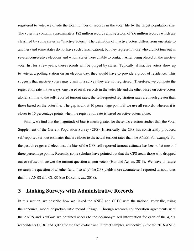
Figure 2: State-level Comparison between the Turnout Rates based on the Voter File and the UnitedStates Election Project. The correlation between these turnout rates is high and the average percentagepoint difference is small.
the 2016 election, in the routine data cleaning processes by states and L2, some of the individuals who
voted in the election might have been removed because they either have deceased or moved (based on
the National Change of Address). As a result, the L2 voter file has a total of 131 million voters who
cast their ballots whereas according to the US Election Project, approximately 136.7 million individuals
voted in the election. In addition, the L2 voter file does not contain overseas voters, reducing the total
VEP size by about 5 million and the turnout rate by slightly more than one percentage point.
Figure 2 compares state-level turnout rates based on the L2 voter file (horizontal axis) with their
corresponding VEP turnout rates from the US Election Project (vertical axis). Recall that deceased voters
and those who moved across states have been removed from the voter file, whereas they are included in
the VEP turnout calculation. As expected, the turnout rate based on the voter file is lower than the actual
turnout. The median difference is 2.7 percentage points whereas the standard deviation is one percentage
point. However, the correlation between the two reaches 0.98. We also find a near perfect correlation at
the county level (see Figure A2 of Appendix A2.1).
We also compute the registration rate using the voter file. Since the voter file lists everyone who is
6
registered to vote, we divide the total number of records in the voter file by the target population size.
The voter file contains approximately 182 million records among a total of 8.6 million records which are
classified by some states as “inactive voters.” The definition of inactive voters differs from one state to
another (and some states do not have such classification), but they represent those who did not turn out in
several consecutive elections and whom states were unable to contact. After being placed on the inactive
voter list for a few years, these records will be purged by states. Typically, if inactive voters show up
to vote at a polling station on an election day, they would have to provide a proof of residence. This
suggests that inactive voters may claim in a survey they are not registered. Therefore, we compute the
registration rate in two ways, one based on all records in the voter file and the other based on active voters
alone. Similar to the self-reported turnout rates, the self-reported registration rates are much greater than
those based on the voter file. The gap is about 10 percentage points if we use all records, whereas it is
closer to 15 percentage points when the registration rate is based on active voters alone.
Finally, we find that the magnitude of bias is much greater for these two election studies than the Voter
Supplement of the Current Population Survey (CPS). Historically, the CPS has consistently produced
self-reported turnout estimates that are closer to the actual turnout rates than the ANES. For example, for
the past three general elections, the bias of the CPS self-reported turnout estimate has been of at most of
three percentage points. Recently, some scholars have pointed out that the CPS treats those who dropped
out or refused to answer the turnout question as non-voters (Hur and Achen, 2013). We leave to future
research the question of whether (and if so why) the CPS yields more accurate self-reported turnout rates
than the ANES and CCES (see DeBell et al., 2018).
3 Linking Surveys with Administrative Records
In this section, we describe how we linked the ANES and CCES with the national voter file, using
the canonical model of probabilistic record linkage. Through research collaboration agreements with
the ANES and YouGov, we obtained access to the de-anonymized information for each of the 4,271
respondents (1,181 and 3,090 for the face-to-face and Internet samples, respectively) for the 2016 ANES
7

as well as 64,600 respondents for the 2016 CCES. We used this information to link the survey data with
the voter file.
3.1 Preprocessing Names and Addresses
As emphasized by Winkler (1995), a key step for a successful merge is to standardize the fields that will
be used to link two datasets. Accordingly, we made every effort to parse the names and addresses used in
the ANES and CCES uniformly so that their formats match with those of the corresponding fields in the
nationwide voter file. For example, the full name of an individual is divided into the first, middle, and
last names, while the address is parsed into house number, street name, zip code, and apartment number
(see Appendix A1.2 for details).
The ANES makes use of data from the United States Postal Service to ensure that the invitation letter
can be delivered to the sampled addresses. As a result, the ANES address data are of high quality. In
contrast, the respondent names are self-reported and each name is represented by a string, which we
parsed into the first, middle, and last names. For self-reported registered voters, whenever available,
we use the name, which they said they had used for registration (3,623 records or 85%). If no name
was provided (either because an individual reported not having registered to vote or failed to provide a
name), we use the name on a check sent as monetary compensation for their participation in the survey
(464 records or 11%). For the remaining respondents, we use the names of individuals whom the ANES
intended to interview (184 records or 4%).
In the case of the CCES, both addresses and names are self-reported. Consequently, we parsed each
name and address for all of the 64,600 respondents and made their format comparable to that of names
and addresses in the nationwide voter file. In the case of names, we followed a similar strategy as the
one used for the ANES by dividing a name string into three components: first, middle, and last names.
However, the names of almost three percent of respondents (1,748 individuals) were missing.
As noted above, the CCES respondents self-report their address as well, and each of those ad-
dresses was stored as a single string variable. We first used preprocText() function in fastLink
8
ANES CCES
All Face-to-face InternetCases % Cases % Cases % Cases %
NamesMissing value(first or last name)
66 1.55 53 4.49 13 0.42 1,748 2.71
Initials for first andlast name
0 0.00 0 0.00 0 0.00 3,274 5.07
Initials for first namebut last name complete
16 0.38 7 0.01 9 0.29 506 0.78
Complete name 4,189 98.07 1,129 95.60 3,068 99.29 59,072 91.44
Addresses
Missing value 0 0.00 0 0.00 0 0.00 7,465 11.55P.O. Box 0 0.00 0 0.00 0 0.00 1,665 2.58
Complete address 4,271 100.00 1,181 100.00 3,090 100.00 55,470 85.87
Number of respondents 4,271 1,181 3,090 64,600
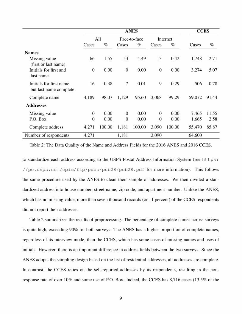
Table 2: The Data Quality of the Name and Address Fields for the 2016 ANES and 2016 CCES.
to standardize each address according to the USPS Postal Address Information System (see https:
//pe.usps.com/cpim/ftp/pubs/pub28/pub28.pdf for more information). This follows
the same procedure used by the ANES to clean their sample of addresses. We then divided a stan-
dardized address into house number, street name, zip code, and apartment number. Unlike the ANES,
which has no missing value, more than seven thousand records (or 11 percent) of the CCES respondents
did not report their addresses.
Table 2 summarizes the results of preprocessing. The percentage of complete names across surveys
is quite high, exceeding 90% for both surveys. The ANES has a higher proportion of complete names,
regardless of its interview mode, than the CCES, which has some cases of missing names and uses of
initials. However, there is an important difference in address fields between the two surveys. Since the
ANES adopts the sampling design based on the list of residential addresses, all addresses are complete.
In contrast, the CCES relies on the self-reported addresses by its respondents, resulting in the non-
response rate of over 10% and some use of P.O. Box. Indeed, the CCES has 8,716 cases (13.5% of the
9
pre-election sample) without any information about names or a valid residential address. This makes it
more challenging to merge the CCES data with the voter file.
3.2 Merge Procedure
Having standardized the linkage fields, we separately merge the ANES and CCES with the nationwide
voter file. Since the nationwide voter file contains more than 180 million records, merging a survey data
set with the voter file all at once would result in a total of over 756 billion and 18 trillion comparisons
for the ANES and CCES, respectively. Therefore, we first subset the survey and voter file data into 102
blocks, defined by state of residence (50 states plus Washington DC) and gender (male and female).
Thus, our merge procedure assumes gender is accurately measured for all voters. Once the within-state
merge is done for each block, we conduct the across-state merge focusing on survey respondents who
are not matched with registered voters through the within-state merge.
In the case of the ANES, the block size ranges from 48,315 pairs (Hawaii/Female: ANES = 3, Voter
file = 16,105) to 705 million pairs (California/Female: ANES = 225, Voter file = 3,137,276) with the
median value of 11 million pairs (Idaho/Male: ANES = 28, Voter file = 426,636). For the CCES, the
block size ranges from more than 3 million (Wyoming/Male: CCES = 45, Voter file = 88,849) to 25
billion pairs (California/Male: CCES = 3,073, Voter file = 8,326,559) with the median value of 301
million pairs (Iowa/Female: CCES = 394, Voter file = 764,169).
Within each block, we conduct the data merge using the following variables: first name, last name,
age, house number, street name, and zip code. We apply the canonical model of probabilistic record
linkage, which was originally proposed by Fellegi and Sunter (1969). Enamorado et al. (2019) improved
the implementation of the algorithm used to fit this model so that it is possible to merge large scale data
sets with millions of records. Throughout the merge process, we use the open-source package fastLink
(Enamorado et al., 2017) to fit the model to our data so that the procedure is transparent.
The model is fit to the data based on the agreement patterns of each linkage field across all possible
pairs of records between the two data sets A and B. We use three levels of agreement for the string
10
valued variables (first name, last name, and street name) based on the Jaro-Winkler similarity measure
with 0.85 and 0.94 as the thresholds (see e.g., Winkler, 1990).6 We also use three levels of agreement for
age based on the absolute distance between values, with 1 and 2.5 years as the thresholds used to separate
agreements, partial agreements, and disagreements (see American National Election Studies (2016) for
a similar choice). For the remaining variables (i.e., house number and postal code), we utilize a binary
comparison indicating whether they have an identical value.
Formally, if we use a binary comparison for variable k, we define γk(i, j) to be a binary variable,
which is equal to 1 if record i in the data set A has the same value as record j in the data set B. If the
variable uses a three-level comparison, then we define γk(i, j) to be a factor variable with three levels,
in which 0, 1, and 2 indicate that the values of two records for this variable are different, similar, and
identical, respectively.
Based on this definition, the record linkage model of Fellegi and Sunter (1969) can be written as
the following two-class mixture model with the latent variable Mij , indicating a match Mij = 1 or a
non-match Mij = 0 for the pair (i, j),
γk(i, j) |Mij = mindep.∼ Discrete(πkm) (1)
Miji.i.d.∼ Bernoulli(λ) (2)
where πkm is a vector of length Lk, which is the number of possible values taken by γk(i, j), containing
the probability of each agreement level for the kth variable given that the pair is a match (m = 1) or
a non-match (m = 0), and λ represents the probability of match across all pairwise comparisons. The
model assumes (1) independence across pairs, (2) independence across linkage fields conditional on the
latent variable Mij , and (3) missing at random conditional on Mij (Enamorado et al., 2019). As shown
in the literature (e.g., Winkler, 1989, 1993; Thibaudeau, 1993; Larsen and Rubin, 2001), it is possible to
6Jaro-Winkler is a commonly used similarity measure for strings. Unlike other alternative measures such as the Lev-enshtein distance and the Jaro similarity, the Jaro-Winkler similarity measure involves a character-wise comparisons with aspecial emphasis on the first characters of the strings being compared.
11

relax this conditional independence assumption using the log-linear model (see Appendix A2.4 for the
results based on this model).
Once the model is fit to the data, we estimate the probability of match using the Bayes rule based on
the maximum likelihood estimates of the model parameters,
ξij = Pr(Mij = 1 | δ(i, j),γ(i, j))
=λ∏K
k=1
(∏Lk−1`=0 π
1{γk(i,j)=`}k1`
)1−δk(i,j)∑1
m=0 λm(1− λ)1−m
∏Kk=1
(∏Lk−1`=0 π
1{γk(i,j)=`}km`
)1−δk(i,j) (3)
where δk(i, j) indicates whether the value of variable k is missing for pair (i, j) (a missing value occurs
if at least one record for the pair is missing the value for the variable).
We say that record j is a potential match of record i if the estimated match probability ξij is the
largest among all pairs that involve record i. Formally, define the following maximum estimated match
probability for record i as follows,
ζi = maxj 6=i
ξij (4)
If there are more than one record whose estimated match probability is equal to ζi, then we randomly
select one of them as a match. Fortunately, in the current applications, there was no tie when ζi is
reasonably high, e.g., ζi ≥ 0.75, and hence random sampling has little effect. This procedure yields
one-to-one match for each respondent i with the estimated match probability of ζi.7
An important concern with our blocking strategy is that we may fail to match an individual whose
residential address has changed between the day of survey interview and the date when our voter file
was updated. It is also possible that people were registered to vote in a residential address different from
the address they reported in the surveys. To identify these individuals, we take all survey respondents
7We examine the robustness of our results by conducting one-to-many matching strategy as described in Enamorado et al.(2019). Specifically, we compute the weighted average of all matched turnout records using the normalized weights that areproportional to the estimated match probabilities. The results are presented in Table A1 of Appendix A2.2 and are essentiallyidentical to the results based on one-to-one match.
12

whose estimated match probability ζi is less than 0.75 and then merge them with registered voters in
other states. There exist a total of 1,100 such respondents for the ANES and 23,585 respondents for the
CCES.
To conduct this across-state merge, we first subset the nationwide voter file such that it only contains
the registered voters whose names are close to the remaining survey respondents. As before, we use the
Jaro-Winkler string distance of 0.94 or above as the threshold. This reduces the number of registered
voters from over 180 million to 14 million. Using fastLink, we find, for each survey respondent, a
registered voter who has the same name (first, middle, and last) and the identical age where the names
with the Jaro-Winkler distance of 0.94 or above are coded as same. This yields 51 and 874 additional
matches for the ANES and CCES, respectively, and for these matches the estimated match probability
is close to 1.8 For those respondents who are not matched, we use the matches from the within-state
merge.9
As an optional final step, we conduct a clerical review (human validation) of each respondent, which
is recommended by some in the literature (e.g., Winkler, 1995), and set the estimated match probability to
zero for those respondents who, our clerical review suggests, do not have a valid match. We caution that a
clerical review may not be useful when the data contain many missing or mismeasured variables. In such
cases, a clerical review may increase false negatives while reducing false positives. In our applications,
as shown in Section 3.1, the names and addresses are more complete for the ANES than for the CCES.
As a result, a clerical review may be more appropriate for the ANES.
Our clerical review discards 284 (8.7% of matches) and 4,115 (9.6% of matches) records as matches
for the ANES and CCES, respectively. For example, 124 cases in the ANES and 2,335 in the CCES
are removed because each of them is matched with an individual in the same household who has the
same name but also has an age difference of more than 5 years and/or do not share a single component
of birthday (day, month or year). This suggests that these matched individual are likely to be relatives.
8Recently, Goel et al. (2019) using synthetic data, found that a merge based just on names and date of birth via fastLinkis able to identify duplicated records across different geographic units with a high degree of precision, even in the presenceof measurement error in the linkage fields.
9Figure A3 of Appendix A2.3 presents the distributions of the estimated match probabilities for the ANES and CCES.
13

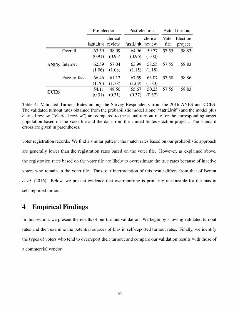
Pre-election Post-election Registration rate
clerical clerical Voter filefastLink review fastLink review all active CPS
ANES
Overall 76.54 68.79 77.15 69.85 80.37 76.57 70.34(0.63) (0.71) (0.67) (0.76) (1.40)
Internet 77.00 69.16 77.77 70.15 80.37 76.57 70.34(0.74) (0.83) (0.79) (0.90) (1.40)
Face-to-face 75.32 67.82 75.64 69.12 80.22 76.43 70.40(1.21) (1.36) (1.27) (1.42) (1.39)
CCES 66.60 58.59 70.52 63.57 80.37 76.57 70.34(0.18) (0.19) (0.19) (0.21) (1.40)
Table 3: Estimated Match Rates from the Results of Merging the ANES and CCES with the Nation-wide Voter File. For the ANES, we compute the match rates separately for the face-to-face and Internetsamples as well as together for the overall sample. Merging is based on the probabilistic model alone(“fastLink”) and the model plus clerical review (“clerical review”). Standard errors are given withinparentheses. For the sake of comparison, we also present the estimated registration rates from the voterfiles (all registered voters “all” and active voters only “active”) as well as the self-reported registrationrate from the Current Population Survey (CPS). Each registration rate is computed for the target popula-tion of corresponding survey estimate.
Similarly, we discard 39 cases in the ANES and 59 in the CCES, where matched individuals have the
same name and age, but a different address and middle name. Finally, we remove 60 cases in the ANES
and 1,404 in the CCES where individuals had the same address and age, but the names were completely
different.
3.3 Estimated Match Rates
To summarize the results of the merge, we estimate the overall match rate as,∑N
i=1 ζi/N where N is the
total number of survey respondents.10 Table 3 presents the match rates for the ANES and CCES using the
pre-election and post-election survey respondents. For the ANES, we present the match rate separately
for the face-to-face and Internet samples as well as for the combined sample (“Overall”). The results
are based on the probabilistic model alone (“fastLink”) and the model plus clerical review (“clerical
review”).10This assumes one-to-one match. Appendix A2.2 relaxes this assumption and presents the results based on one-to-many
maches.
14
For the sake of comparison, we also present the two estimates of registration rate based on the voter
file for the target populations for surveys. The first (“all”) is the total number of voters in the voter file
divided by the number of eligible voters. However, these registration rates are likely to overestimate the
true rates because some voters may have deceased or moved. For this reason, as explained earlier, in
some (but not all) states, the Secretary of State office labels voters “inactive” before purging them from
the voter file. The second estimate (“active”) uses the total number of active voters as the numerator.
Since the exact definition of active voters varies by states and some states do not distinguish active
and inactive voters, these estimates may not approximate the actual registration rate. It is possible that
survey respondents may think they are registered even though they are classified as inactive voters or
even removed from the voter file. In the final column, we also present the estimated registration rate
based on self-reports from the CPS.
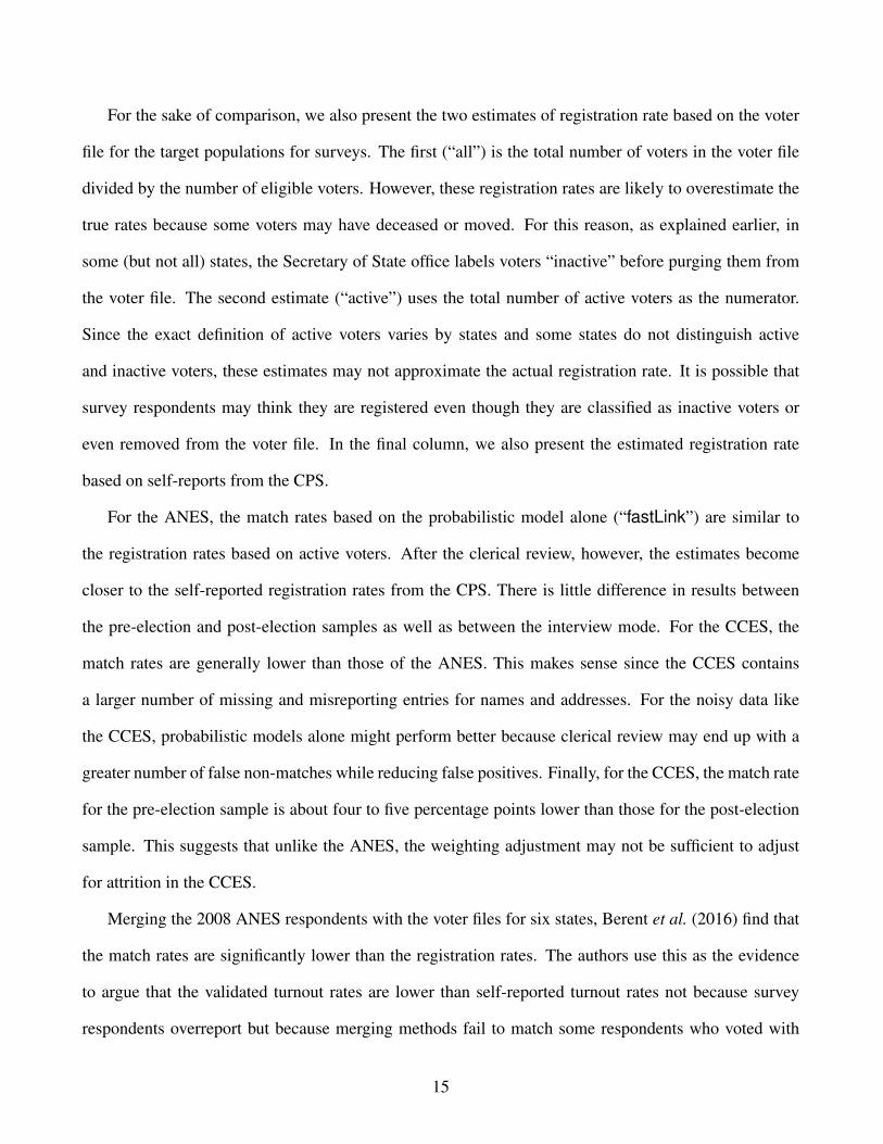
For the ANES, the match rates based on the probabilistic model alone (“fastLink”) are similar to
the registration rates based on active voters. After the clerical review, however, the estimates become
closer to the self-reported registration rates from the CPS. There is little difference in results between
the pre-election and post-election samples as well as between the interview mode. For the CCES, the
match rates are generally lower than those of the ANES. This makes sense since the CCES contains
a larger number of missing and misreporting entries for names and addresses. For the noisy data like
the CCES, probabilistic models alone might perform better because clerical review may end up with a
greater number of false non-matches while reducing false positives. Finally, for the CCES, the match rate
for the pre-election sample is about four to five percentage points lower than those for the post-election
sample. This suggests that unlike the ANES, the weighting adjustment may not be sufficient to adjust
for attrition in the CCES.
Merging the 2008 ANES respondents with the voter files for six states, Berent et al. (2016) find that
the match rates are significantly lower than the registration rates. The authors use this as the evidence
to argue that the validated turnout rates are lower than self-reported turnout rates not because survey
respondents overreport but because merging methods fail to match some respondents who voted with
15
Pre-election Post-election Actual turnout
clerical clerical Voter ElectionfastLink review fastLink review file project
ANES
Overall 63.59 58.09 64.96 59.77 57.55 58.83(0.91) (0.93) (0.96) (1.00)
Internet 62.59 57.04 63.99 58.55 57.55 58.83(1.06) (1.08) (1.15) (1.18)
Face-to-face 66.46 61.12 67.59 63.07 57.58 58.86(1.76) (1.78) (1.69) (1.83)
CCES 54.11 48.50 55.67 50.25 57.55 58.83(0.31) (0.31) (0.37) (0.37)
Table 4: Validated Turnout Rates among the Survey Respondents from the 2016 ANES and CCES.The validated turnout rates obtained from the probabilistic model alone (“fastLink”) and the model plusclerical review (“clerical review”) are compared to the actual turnout rate for the corresponding targetpopulation based on the voter file and the data from the United States election project. The standarderrors are given in parentheses.
voter registration records. We find a similar pattern: the match rates based on our probabilistic approach
are generally lower than the registration rates based on the voter file. However, as explained above,
the registration rates based on the voter file are likely to overestimate the true rates because of inactive
voters who remain in the voter file. Thus, our interpretation of this result differs from that of Berent
et al. (2016). Below, we present evidence that overreporting is primarily responsible for the bias in
self-reported turnout.
4 Empirical Findings
In this section, we present the results of our turnout validation. We begin by showing validated turnout
rates and then examine the potential sources of bias in self-reported turnout rates. Finally, we identify
the types of voters who tend to overreport their turnout and compare our validation results with those of
a commercial vendor.
16
4.1 Validated Turnout Rates
To obtain the validated turnout rate, we compute the weighted average of the binary turnout variable
among matched voters in the voter file where the estimated match probability ζi is used as the (un-
normalized) weight. Table 4 presents the validated turnout rates among the survey respondents from
the pre-election and post-election surveys of the 2016 ANES and CCES. As in Table 3, we compare
the results obtained from the probabilistic model alone (“fastLink”) and the model plus clerical review
(“clerical review”) with actual turnout rates based on the voter file (“Voter file”) and the United States
election project (“Election project”). The standard errors that account for sampling design and unit
non-response, are given in parentheses.
Our main findings about turnout rates are consistent with those about registration rates given in
Table 3. For the ANES, the validated turnout rates directly obtained from fastLink are at least five
percentage points greater than the actual turnout rates. However, clerical review helps close this gap,
yielding the validated turnout rates that are within the sampling error of the actual turnout rates. For the
sample of face-to-face interview, the validated turnout rates are higher than the Internet sample though
the standard errors are greater.11
For the CCES, the validated turnout rates directly obtained from fastLink are closer to the actual
turnout rates than those based on the model and clerical review. The reason for this difference is the
same as the one discussed earlier. Because the CCES contains many misreported and missing entries
especially for addresses, clerical review ends up removing the potential matches involving these records
and hence introducing false negatives. This suggests that clerical review may be ineffective for noisy
data. We also note that the validated turnout rates based on the model and clerical review are similar to
the result obtained by YouGov based on a voter file provided by a commercial firm, Catalist.
We conduct several robustness checks. First, we compare the results based on one-to-one match-
ing strategy with those based on one-to-many matching strategy described in Enamorado et al. (2019).
11See Appendix A1.4 for more details about the different sampling weights of the ANES and CCES.
17
Table A1 of Appendix A2.2 shows that these results are essentially identical. Second, Appendix A2.4
presents the results from the log-linear model that does not require the conditional independence as-
sumption. Although the substantive results are similar, the resulting matched and validated turnout rates
are somewhat lower than those obtained under the conditional independence assumption. Finally, Ap-
pendix A3 further compares our validated turnout with that based on the vote validation conducted for
the CCES using data from Catalist and a proprietary algorithm. Overall, we find that fastLink performs
at least as well as an state-of-the-art proprietary algorithm (see Appendix A3 for more details).
4.2 Possible Sources of Bias in Self-reported Turnout
What are the possible sources of differences between self-reported and validated turnout rates? The
literature suggests overreporting, attrition, and mobilization as the main culprits. Below, we show that
overreporting accounts for more than 90% of the bias of self-reported turnout, while non-response due to
attrition plays a smaller role. Unfortunately, unlike Jackman and Spahn (2019), we cannot examine the
contribution of mobilization to the bias of self-reported turnout because of a design difference between
the 2012 and 2016 ANES face-to-face surveys.
4.2.1 Misreporting
We first consider overreporting as a potential source of bias in self-reported turnout. Table 5 presents
the validated turnout rates among survey respondents with different responses to the turnout questions
of the ANES and CCES. We find that about 20% of the ANES respondents who said they had voted in
the post-election survey did not turn out according to the voter file, whereas the corresponding estimated
proportion of overreporting for the CCES is about 30%. Compared to the probabilistic model alone
(“fastLink”), the use of clerical review (“clerical review”) increases the estimated overreporting rate
by several percentage points for both surveys. Because a majority of respondents said they had voted
(78% for the ANES and 85% for the CCES), overreporting is mostly responsible for the upward bias in
self-reported turnout.
In terms of underreporting, the results from fastLink show that approximately 69 voters or 15% (109
18
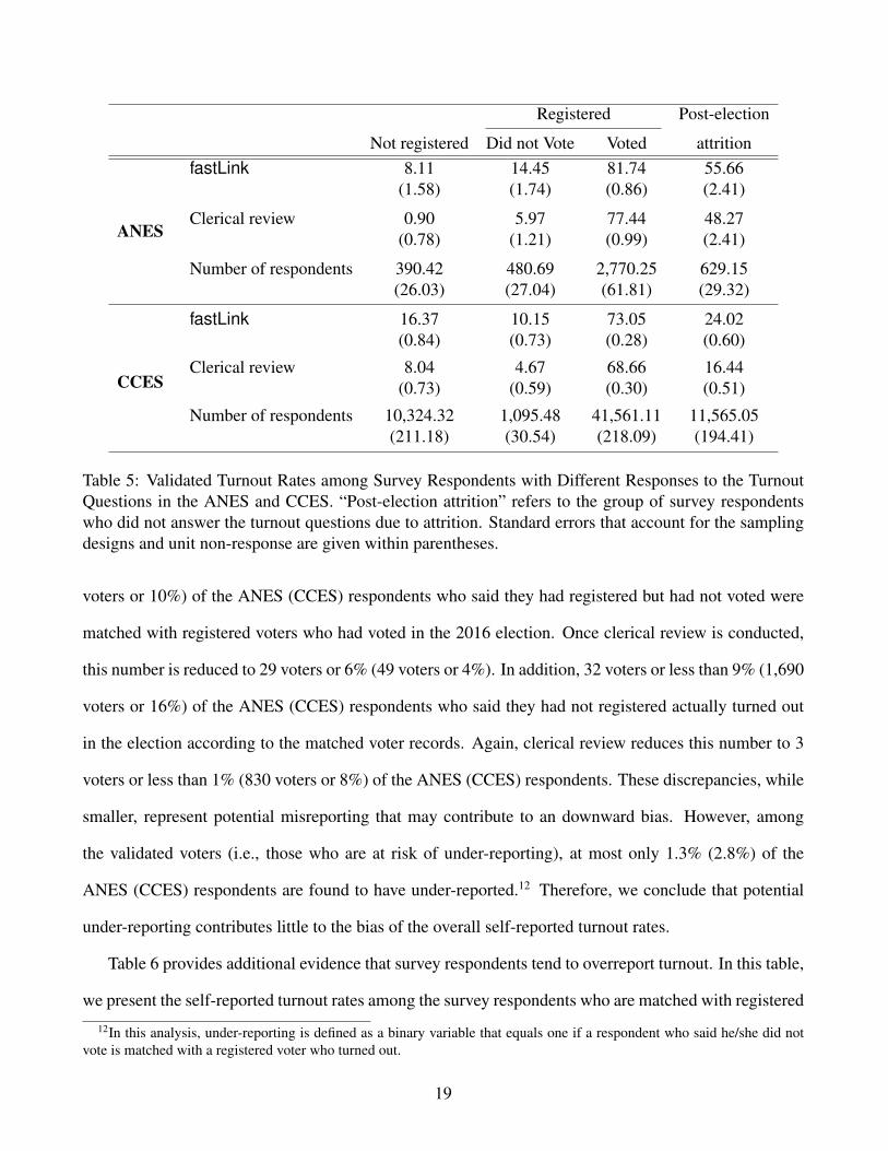
Registered Post-election
Not registered Did not Vote Voted attrition
ANES
fastLink 8.11 14.45 81.74 55.66(1.58) (1.74) (0.86) (2.41)
Clerical review 0.90 5.97 77.44 48.27(0.78) (1.21) (0.99) (2.41)
Number of respondents 390.42 480.69 2,770.25 629.15(26.03) (27.04) (61.81) (29.32)
CCES
fastLink 16.37 10.15 73.05 24.02(0.84) (0.73) (0.28) (0.60)
Clerical review 8.04 4.67 68.66 16.44(0.73) (0.59) (0.30) (0.51)
Number of respondents 10,324.32 1,095.48 41,561.11 11,565.05(211.18) (30.54) (218.09) (194.41)
Table 5: Validated Turnout Rates among Survey Respondents with Different Responses to the TurnoutQuestions in the ANES and CCES. “Post-election attrition” refers to the group of survey respondentswho did not answer the turnout questions due to attrition. Standard errors that account for the samplingdesigns and unit non-response are given within parentheses.
voters or 10%) of the ANES (CCES) respondents who said they had registered but had not voted were
matched with registered voters who had voted in the 2016 election. Once clerical review is conducted,
this number is reduced to 29 voters or 6% (49 voters or 4%). In addition, 32 voters or less than 9% (1,690
voters or 16%) of the ANES (CCES) respondents who said they had not registered actually turned out
in the election according to the matched voter records. Again, clerical review reduces this number to 3
voters or less than 1% (830 voters or 8%) of the ANES (CCES) respondents. These discrepancies, while
smaller, represent potential misreporting that may contribute to an downward bias. However, among
the validated voters (i.e., those who are at risk of under-reporting), at most only 1.3% (2.8%) of the
ANES (CCES) respondents are found to have under-reported.12 Therefore, we conclude that potential
under-reporting contributes little to the bias of the overall self-reported turnout rates.
Table 6 provides additional evidence that survey respondents tend to overreport turnout. In this table,
we present the self-reported turnout rates among the survey respondents who are matched with registered
12In this analysis, under-reporting is defined as a binary variable that equals one if a respondent who said he/she did notvote is matched with a registered voter who turned out.
19

Voters Non-voters
% Cases % Cases Total
ANES
fastLink 95.68 2,436 33.66 378 2,814(0.50) (3.01)
Clerical review 98.50 2,258 30.84 290 2,548(0.32) (3.48)
CCES
fastLink 92.70 33,329 43.49 3,901 37,230(0.36) (1.25)
Clerical review 96.33 30,741 44.35 2,836 33,577(0.32) (1.75)
Table 6: Self-Reported Turnout Rates among Matched Voters and Non-voters. In the “Voters” (“Non-voters”) column, we present the self-reported turnout rate among the survey respondents who are vali-dated to have voted (have abstained) in the 2016 election. More than 30% (40%) of the ANES (CCES)survey responded who did not vote reported they had voted. Standard errors are given within parentheses.
voters in the voter file. For the results based on fastLink without clerical review, we use the estimated
match probability as described in equation (4) to weight each observation.
Although misreporting is almost non-existent among those who are validated to have voted, more
than 30% (40%) of the participants of the ANES (CCES) who self-reported to have voted did not ac-
tually vote according to their matched record in the voter file. This finding is consistent with that of
Ansolabehere and Hersh (2012). While matched non-voters may differ from non-voters who are not
matched, our finding suggests that the unmatched non-voters may also overreport their turnout, leading
to a substantial overreporting. Our finding contradicts the claim put forth by Berent et al. (2016) that
survey respondents do not often overreport turnout. These authors show that matched respondents tend
not to overreport. However, they did not separate matched voters from matched non-voters, and as a
result overlooked the tendency of matched non-voters to overreport.
4.2.2 Attrition
Next, we examine the consequences of attrition. The last column of Table 5 presents the validated
turnout among those who dropped out after the pre-election survey and did not answer the post-election
survey. The validated turnout rate for the ANES dropouts is similar to the overall turnout, suggesting that
attrition does not substantially bias the results. For the CCES, those who did not answer the post-election
20
survey have a much lower validated turnout rate, implying that attrition may have contributed to the bias
of self-reported turnout.
This pattern is consistent with Table 4, which shows the similarity of the validated turnout rates
between the pre-election and post-election surveys for the ANES, but not for the CCES. In contrast with
some previous work in the literature (e.g., Burden, 2000), this finding suggests that attrition is unlikely
to explain the gap between the self-reported and actual turnout rates for the ANES though it may be
responsible for some, but not all, of the bias for the CCES. Sampling weights of the ANES appear to be
able to properly adjust for the possible bias due to unit and item non-response.13
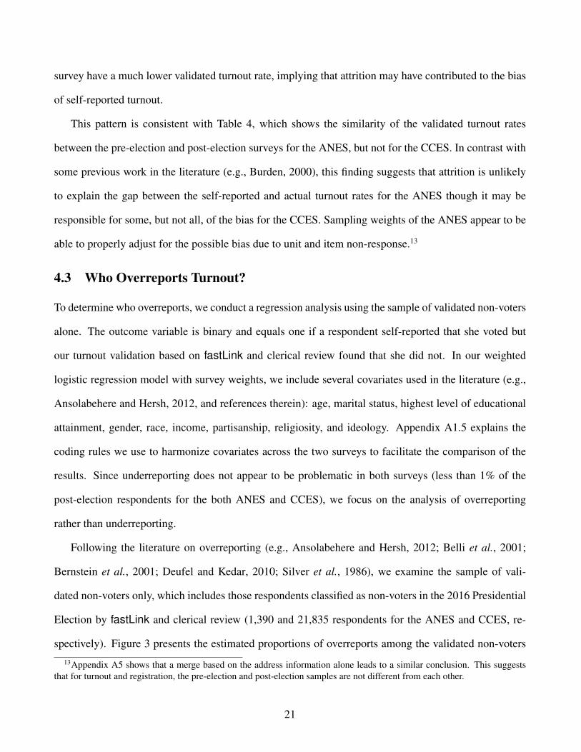
4.3 Who Overreports Turnout?
To determine who overreports, we conduct a regression analysis using the sample of validated non-voters
alone. The outcome variable is binary and equals one if a respondent self-reported that she voted but
our turnout validation based on fastLink and clerical review found that she did not. In our weighted
logistic regression model with survey weights, we include several covariates used in the literature (e.g.,
Ansolabehere and Hersh, 2012, and references therein): age, marital status, highest level of educational
attainment, gender, race, income, partisanship, religiosity, and ideology. Appendix A1.5 explains the
coding rules we use to harmonize covariates across the two surveys to facilitate the comparison of the
results. Since underreporting does not appear to be problematic in both surveys (less than 1% of the
post-election respondents for the both ANES and CCES), we focus on the analysis of overreporting
rather than underreporting.
Following the literature on overreporting (e.g., Ansolabehere and Hersh, 2012; Belli et al., 2001;
Bernstein et al., 2001; Deufel and Kedar, 2010; Silver et al., 1986), we examine the sample of vali-
dated non-voters only, which includes those respondents classified as non-voters in the 2016 Presidential
Election by fastLink and clerical review (1,390 and 21,835 respondents for the ANES and CCES, re-
spectively). Figure 3 presents the estimated proportions of overreports among the validated non-voters
13Appendix A5 shows that a merge based on the address information alone leads to a similar conclusion. This suggeststhat for turnout and registration, the pre-election and post-election samples are not different from each other.
21
Education
Proportion of Over−reporting (%)0 20 40 60 80 100
High school or less
Some college
College
Post− graduate
High school or less
Some college
College
Post− graduate
CC
ES
AN
ES
Income (in thousands)
Proportion of Over−reporting (%)0 20 40 60 80 100
Less than 27.5
Between 27.5 and 60
Between 60 and 100
More than 100
Less than 30
Between 30 and 60
Between 60 and 100
More than 100
CC
ES
AN
ES
Interest in Politics
Proportion of Over−reporting (%)0 20 40 60 80 100
A lot
Some
Not much
Not at all
A lot
Some
Not much
Not at all
CC
ES
AN
ES
Partisanship
Proportion of Over−reporting (%)0 20 40 60 80 100
Democrat
Republican
Independent
Democrat
Republican
Independent
CC
ES
AN
ES
Race
Proportion of Over−reporting (%)0 20 40 60 80 100
Black
White
Hispanic
Other
Black
White
Hispanic
Other
CC
ES
AN
ES
Church Attendance
Proportion of Over−reporting (%)0 20 40 60 80 100
Frequently
A few times a year
Rarely/Never
Frequently
A few times a year
Rarely/Never
CC
ES
AN
ES
Figure 3: Estimated Proportion of Overreporting across Different Covariates in the Sample of ValidatedNon-Voters. The results are based on the weighted logistic regression separately fitted to the CCES (lightblue) and ANES (dark blue) samples of validated non-voters. Each plot presents the estimated proportionof overreporting averaging over the entire sample of validated non-voters while fixing the other covariatesat their observed values. Nonresponse is treated as a separate category for each covariate.
across the different values of some covariates, whose coefficients are estimated to be statistically signifi-
cantly different from zero. These estimates are obtained by averaging over all respondents in the sample
of validated non-voters (using the sampling weights) while fixing the other covariates to their observed
22
values. Thus, each estimated regression coefficient represents the predicted difference in over-reporting
between two individuals who share all the observed characteristics except the corresponding covariate.
Here, we graphically summarize the results, while the estimated coefficients and their standard errors
are given in Table A4 of Appendix A2.5.14 For both the ANES and CCES, we find similar patterns:
educated respondents tend to overreport more than the uneducated, partisans are more likely to overre-
port than independents, and those who said they were interested in politics overreport more than those
with little interest.15 Although the overall pattern is similar between the two surveys, there are some
small differences. For example, for the CCES, there is a monotonic relationship between income and
overreporting: respondents with high income tend to overreport more than poor respondents. However,
for the ANES, the relationship is not monotonic. In addition, for the ANES, we find a substantial dif-
ference in the propensity to overreport turnout between African Americans and the other voters whereas
the magnitude of this difference is much smaller for the CCES.
These results are in line with the findings of other validation studies that have used ANES data and
proprietary record linkage algorithms. For example, previous studies have also found that those who are
more partisan (e.g., Ansolabehere and Hersh, 2012), interested in politics (e.g., Ansolabehere and Hersh,
2012; Bernstein et al., 2001), educated (e.g., Ansolabehere and Hersh, 2012; Bernstein et al., 2001) and
wealthier (e.g., Ansolabehere and Hersh, 2012) are likely to overreport turnout. In addition, our findings
are consistent with the existing studies that show African Americans are more likely to overreport if
compared to other racial groups (e.g., Traugott and Katosh, 1979; Abramson and Claggett, 1992; Belli
et al., 2001; Bernstein et al., 2001; Deufel and Kedar, 2010). However, unlike some older studies such
as Silver et al. (1986) and Bernstein et al. (2001), our results do not show a strong relationship between
overreporting and age, and overreporting and religiosity. These discrepancies may arise in part because
14Appendix A2.6 presents a bivariate analysis of overreporting. We focus on two outcomes, the proportion and the odds-ratio of overreporting for the different values taken by each covariate commonly used to explain who is more likely tooverreports. The bivariate analysis recovers the patterns similar to the ones obtained by the multivariate regression analysis(see Tables A6 and A7).
15In addition, Table A5 of Appendix A2.5 presents the results concerning the determinants of overreporting for the ANESsample separately for each interview mode. The patterns observed using the complete sample are quite similar to those byfocusing on the face-to-face and internet samples of the ANES.
23
the nature of over-reporting may have possibly changed over time. Additional validation studies are
needed to further investigate these differences.
5 Concluding Remarks
Over the last decade, the availability of large-scale electronic administrative records enabled researchers
to study important questions by creatively merging them with other data sets (see e.g., Jutte et al., 2011;
Ansolabehere and Hersh, 2012; Einav and Levin, 2014). A major methodological challenge of these
studies, however, is that there often exists no unique identifier that can be used to unambiguously merge
data sets. In these situations, probabilistic record linkage methods that have been developed in the
statistics literature over the last several decades can serve as a useful methodological tool.
This paper presents a case study that applies the canonical record linkage method of Fellegi and
Sunter (1969) to merge two prominent national election survey data sets with the nationwide voter file of
more than 180 million records. We show that the recent computational improvements makes it possible
to conduct this large-scale data merge. Unlike the previous studies which relied upon proprietary algo-
rithms, we use the newly developed open-source software package, facilitating the transparency, repli-
cability, and falsifiability of scientific studies. Our analysis demonstrates that the probabilistic record
linkage method can successfully validate turnout and shed light on the debate regarding the potential
causes of bias in self-reported turnout. The probabilistic method is especially effective dealing with
missing and invalid entries as shown in the case of the CCES validation. We believe that a similar ap-
plication of probabilistic record linkage methods in other domains can also be fruitful, leading to new
scientific discoveries.
Finally, an important implication is that when designing surveys one could anticipate the potential
difficulties that arise while merging survey data with administrative records. In particular, one could
maximize the accuracy of measurements that are used for linking records. For example, the complete
address records of the ANES played an important role in its successful turnout validation. In addition,
if a survey has multiple ways like the ANES and CCES, one could merge the first wave and verify the
24

necessary information in subsequent waves.
References
Abramson, P. and Claggett, W. (1992). The quality of record keeping and racial differences in validated
turnout. Journal of Politics 54, 3, 871–880.
American Association for Public Opinion Research (2017). An evalution of 2016 election polls in the
United States. Tech. rep., Ad Hoc Committee on 2016 Election Polling.
American National Election Studies (2016). User’s guide and codebook for the anes 2012 time series
voter validation supplemental data. Tech. rep., University of Michigan and Stanford University, Ann
Arbor, MI and Palo Alto, CA.
Ansolabehere, S. and Hersh, E. (2012). Validation: What big data reveal about survey misreporting and
the real electorate. Political Analysis 20, 4, 437–459.
Belli, R., Traugott, M., and Beckmann, M. (2001). What leads to voting overreports? contrasts of
overreporters to validated voters and admitted nonvoters in the american national election studies.
Journal of Official Statistics 17, 4, 479–498.
Berent, M. K., Krosnick, J. A., and Lupia, A. (2011). The quality of government records and “over-
estimation” of registration and turnout in surveys: Lessons from the 2008 ANES panel study’s regis-
tration and turnout validation exercises. Tech. Rep. nes012554, American National Election Studies,
Ann Arbor, Michigan and Palo Alto, California.
Berent, M. K., Krosnick, J. A., and Lupia, A. (2016). Measuring voter registration and turnout in surveys.
Public Opinion Quarterly 80, 3, 597–621.
Bernstein, R., Chadha, A., and Montjoy, R. (2001). Overreporting voting: Why it happens and why it
matters. Public Opinion Quarterly 65, 1, 22–44.
25

Burden, B. (2000). Voter turnout and the national election studies. Political Analysis 8, 4, 389–398.
DeBell, M., Krosnick, J. A., Gera, K., Yeager, D. S., and McDonald, M. P. (2018). The turnout gap in
surveys: Explanations and solutions. Sociological Methods & Research forthcoming.
Deufel, B. and Kedar, O. (2010). Race and turnout in u.s. elections exposing hidden effects. Public
Opinion Quarterly 74, 2, 286–318.
Einav, L. and Levin, J. (2014). Economics in the age of big data. Science 346, 6210.
Enamorado, T., Fifield, B., and Imai, K. (2017). fastlink: Fast probabilistic record linkage. avail-
able at the Comprehensive R Archive Network (CRAN). https://CRAN.R-project.org/
package=fastLink.
Enamorado, T., Fifield, B., and Imai, K. (2018a). User’s guide and codebook for the ANES 2016 time
series voter validation supplemental data. Tech. rep., American National Election Studies.
Enamorado, T., Fifield, B., and Imai, K. (2018b). User’s guide and codebook for the CCES 2016 voter
validation supplemental data. Tech. rep., Cooperative Congressional Election Study.
Enamorado, T., Fifield, B., and Imai, K. (2019). Using a probabilistic model to assist merging of large-
scale administrative records. American Political Science Review 113, 2, 353–371.
Enns, P. K., Lagodny, J., and Schuldt, J. P. (2017). Understanding the 2016 US presidential polls: The
importance of hidden Trump supporters. Statistics, Politics, and Policy 8, 1, 41–63.
Fellegi, I. P. and Sunter, A. B. (1969). A theory of record linkage. Journal of the American Statistical
Association 64, 328, 1183–1210.
Goel, S., Meredith, M., Morse, M., Rothschild, D., and Shirani-Mehr, H. (2019). One person, one vote:
Estimating the prevalence of double voting in u.s. presidential elections. University of Pennsylvania,
technical report.
26

Hur, A. and Achen, C. (2013). Coding voter turnout responses in the current population survey. Public
Opinion Quarterly. 77, 4, 985–993.
Jackman, S. and Spahn, B. (2019). Why does the american national election study overestimate voter
turnout? Political Analysis 27, 2, 193–207.
Jutte, D. P., Roos, L. L., and Browne, M. D. (2011). Administrative record linkage as a tool for public
health research. Annual Review of Public Health 32, 91–108.
Lahiri, P. and Larsen, M. D. (2005). Regression analysis with linked data. Journal of the American
Statistical Association 100, 469, 222–230.
Larsen, M. D. and Rubin, D. B. (2001). Iterative automated record linkage using mixture models. Journal
of the American Statistical Association 96, 453, 32–41.
McDonald, M. P. and Popkin, S. L. (2001). The myth of the vanishing voter. American Political Science
Review 95, 4, 963–974.
Silver, B. D., Anderson, B. A., and Abramson, P. R. (1986). Who overreports voting? American Political
Science Review 80, 2, 613–624.
Thibaudeau, Y. (1993). The discrimination power of dependency structures in record linkage. Survey
Methodology. 31–38.
Traugott, M. and Katosh, J. (1979). Response validity in surveys of voting behavior. Public Opinion
Quarterly 43, 3, 359–377.
Winkler, W. E. (1989). Near automatic weight computation in the fellegi-sunter model of record linkage.
Tech. rep., Proceedings of the Census Bureau Annual Research Conference.
Winkler, W. E. (1990). String comparator metrics and enhanced decision rules in the fellegi-sunter model
of record linkage. Proceedings of the Section on Survey Research Methods. American Statistical
Association.
27

Winkler, W. E. (1993). Improved decision rules in the fellegi-sunter model of record linkage. In Pro-
ceedings of Survey Research Methods Section, American Statistical Association.
Winkler, W. E. (1995). Business Survey Methods, chap. Matching and Record Linkage, 355–84. New
York: J. Wiley.
Winkler, W. E. (2006). Overview of record linkage and current research directions. Tech. rep., United
States Bureau of the Census.
28
Top Related